the selection of appropriate spectrally bright pseudo-invariant ground targets for use in empirical...

ISPRS Journal of Photogrammetry and Remote Sensing 66 (2011) 429–445

Contents lists available at ScienceDirect

ISPRS Journal of Photogrammetry and Remote Sensing

journal homepage: www.elsevier.com/locate/isprsjprs

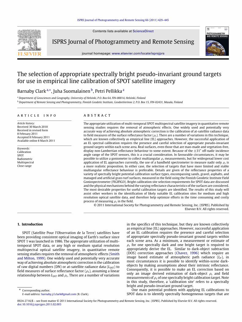
The selection of appropriate spectrally bright pseudo-invariant ground targetsfor use in empirical line calibration of SPOT satellite imageryBarnaby Clark a,∗, Juha Suomalainen b, Petri Pellikka a

a Department of Geosciences and Geography, University of Helsinki, P.O. Box 64, FIN-00014, Helsinki, Finlandb Department of Remote Sensing and Photogrammetry, Finnish Geodetic Institute, Geodeetinrinne 2, P.O. Box 15, FIN-02431, Masala, Finland

a r t i c l e i n f o

Article history:Received 30 March 2010Received in revised form8 February 2011Accepted 8 February 2011Available online 8 March 2011

Keywords:CalibrationSPOTRadiometricMultispectralClose range

a b s t r a c t

The appropriate utilization ofmulti-temporal SPOTmultispectral satellite imagery in quantitative remotesensing studies requires the removal of atmospheric effects. One widely used and potentially veryaccurate way of achieving absolute atmospheric correction is the calibration of at-satellite radiance datato field measures of the surface reflectance factor (ρs). There are a number of variations in this technique,which are known collectively as empirical line (EL) approaches. However, the successful application ofan EL spectral calibration requires the presence and careful selection of appropriate pseudo-invariantground targets within each scene area. Real surfaces, even those that are man-made and vegetation-free,display non-Lambertian reflectance behaviour to some extent. Because of the ±31° off-nadir incidenceangle range of the SPOT sensors, this is a crucial consideration. In favourable circumstances, it may bepossible to utilize a goniometer to collect multiangular ρs measurements, but for widespread lower costapplication of EL approaches currently, the use of a handheld spectrometer to measure nadir only ρs isa more realistic proposition. In either case, the selection of targets that have more limited and stablemultiangular reflectance behaviour is preferable. Details are given of the reflectance properties of avariety of spectrally bright potential calibration surface types, encompassing sands, gravel, asphalts, andmanaged and artificial grass turf surfaces, measured in the field using the Finnish Geodetic Institute FieldGoniospectrometer (FIGIFIGO). Bright calibration site selection requirements for SPOT data are discussedand the physicalmechanisms behind the varying reflectance characteristics of the surfaces are considered.The most desirable properties for useful calibration targets are identified. The results of this study willassist other workers in the identification of likely suitable EL calibration sites for medium and highresolution optical satellite data, and therefore help optimize efforts in the time consuming and costlyprocess of measuring ρs in the field.

© 2011 International Society for Photogrammetry and Remote Sensing, Inc. (ISPRS). Published byElsevier B.V. All rights reserved.

1. Introduction

SPOT (Satellite Pour l’Observation de la Terre) satellites havebeen providing consistent optical imaging of Earth’s surface sinceSPOT 1 was launched in 1986. The appropriate utilization of multi-temporal SPOT data, or any high or medium spatial resolutionmultispectral optical satellite imagery, in quantitative remotesensing studies requires the removal of atmospheric effects (Smithand Milton, 1999). One widely used and potentially very accurateway of achieving absolute atmospheric correction is the calibrationof raw digital numbers (DN) or at-satellite radiance data (LSAT) tofield measures of surface reflectance factor (ρs), assuming a linearrelationship between LSAT and ρs. There are a number of variations

∗ Corresponding author.E-mail address: [email protected] (B. Clark).

0924-2716/$ – see front matter© 2011 International Society for Photogrammetry anddoi:10.1016/j.isprsjprs.2011.02.003

in the specifics of this technique, but they are known collectivelyas empirical line (EL) approaches. However, successful applicationof an EL calibration requires the presence and careful selectionof appropriate spectrally pseudo-invariant ground targets withineach scene area. As a minimum, a measurement or estimate ofρs for one spectrally dark and one bright target is required toappropriately derive the EL. Similar to dark-object subtraction(DOS) correction approaches (Chavez, 1996) which require animage based estimate of atmospheric path radiance (LP ), inmost circumstances it is possible to identify within-scene dark-objects by making assumptions about their intrinsic reflectance.Consequently, it is possible to make an EL correction based ononly an image derived estimation of dark-object ρs and fieldmeasurements ofρs of one spectrally bright calibration target. Notein this study, therefore, a ‘calibration site’ refers to a spectrallybright and pseudo-invariant ground target.

One main potential problem with applying EL calibrations toSPOT data is to identify spectrally homogeneous targets that are

Remote Sensing, Inc. (ISPRS). Published by Elsevier B.V. All rights reserved.

http://dx.doi.org/10.1016/j.isprsjprs.2011.02.003

http://www.elsevier.com/locate/isprsjprs

http://www.elsevier.com/locate/isprsjprs

mailto:[email protected]

http://dx.doi.org/10.1016/j.isprsjprs.2011.02.003

430 B. Clark et al. / ISPRS Journal of Photogrammetry and Remote Sensing 66 (2011) 429–445

Table 1Site details of the potential HELM calibration targets.

# Site name Site location Surface type Measurement dates

1 Hietsu beach 60°10′28′′ N Medium sanda 13.09.200524°54′28′′ E 17.07.2006

08.06.20072 Vermo car park 60°12′52′′ N Asphalt 20.05.2005

24°50′22′′ E 25.05.200505.07.2005

3 Pasila sports ground 60°12′29′′ N Very fine gravela 07.06.200524°56′39′′ E 13.09.2005

4 Pasila velodrome 60°12′10′′ N Artificial turf 04.06.200724°56′35′′ E 07.06.2007

5 Malmi airfield 60°15′00′′ N Asphalt 04.06.200725°02′41′′ E

6 Töölö soccer pitch turf 60°11′11′′ N Managed grass 19.07.200624°55′26′′ E 05.06.2007

7 Kumpula sports ground 60°12′50′′ N Very coarse sanda 13.09.200524°58′09′′ E

8 Pasila baseball ground 60°12′23′′ N Very coarse sanda 07.06.200524°56′31′′ E 13.09.2005

a Aggregate classes as described by the Wentworth (1922) scale.

of sufficient spatial extent to counter radiometric ‘contamination’from adjacency effects, and from the point spread function (PSF)of the ground instantaneous field-of-view (GIFOV) of the sensors.Furthermore, real surfaces, even those man-made and vegetation-free, display non-Lambertian reflectance behaviour to someextent.This is a crucial consideration for SPOT data because of the ±31°off-nadir incidence angle (θV ) range of the sensors.

In favourable circumstances, it may be possible to utilize agoniometer to collect multiangular ρs measurements, but forwidespread lower cost application of EL approaches currently, useof a handheld spectrometer tomeasure nadir onlyρs is amore real-istic proposition. In either case, selection of calibration targets thathavemore limited and stablemultiangular reflectance behaviour ispreferable. Bannari et al. (2005) suggested that spectral measure-ment of stable sites should derive a spatial coefficient of variation(CV) of ≤3%, a criterion that was also utilized by de Vries et al.(2007). Further, Schroeder et al. (2006) stated that a benchmarkfor establishing successful absolute atmospheric correction of op-tical satellite imagery in the visible/near-infrared (VIS/NIR) bandsis an absolute accuracy of ±0.02ρs. These figures can also be usedas a basis for judging significant variations in spectral properties.

Based onworking in ancillary data limited circumstances, Clarkand Pellikka (2009) developed the historical empirical line method(HELM) specifically for SPOT data (see also Clark, 2010; Clark et al.,2011). For implementations on multi-temporal imagery datasets,HELM makes an assumption of calibration target stability overtime and consequently has more stringent requirements than anEL calibrationmade to overpass concurrent ρs fieldmeasurements.The objective of this study is, therefore, to investigate thecharacteristics of, and physical mechanisms behind, multiangular,spatial and temporal ρs variations for potential HELM calibrationtargets. The Finnish Geodetic Institute Field Goniospectrometer(FIGIFIGO; Suomalainen et al., 2009) was utilized to investigatethe ρs properties of a variety of potential HELM calibration surfacetypes, encompassing sands, gravel, asphalts, managed grass turf,and an artificial grass surface, occurring within the Helsinkimetropolitan region study area. The actual application of HELMto the SPOT data, and accuracy assessment and comparisonswith other atmospheric correction methods applicable in thesame intended usage circumstances, form further research workdetailed in Clark et al. (2010, 2011).

2. Methods

2.1. Study area

The Helsinki metropolitan region is situated at 60°12′ N,24°56′ E along the Baltic coastline of southern Finland. Average

temperatures fall below 0 °C from December until March (FinnishMeteorological Institute: www.fmi.fi), with snow cover likelythroughout this period. The area is topographically flat, witha near sea-level elevation, and has extensive urbanization anddevelopment as well as agricultural areas, lakes and forests.

2.2. Finnish Geodetic Institute Field Goniospectrometer (FIGIFIGO)measurements

FIGIFIGO (Suomalainen et al., 2009) was used to take detailedmultiangular daylight ρs measurements of different surface typesas candidates for HELM calibration sites. Following preliminaryidentification in Google EarthTM, eight sites were visited in thefield and deemed suitable for data collection (Table 1). The majorconstraint in data acquisitionwas the limited northern hemispherespring/summer measurement window and the requirement forsustained cloud-free weather conditions. This made planningand execution of a coherent sampling strategy very difficult andconsequently data was collected over a period of 3 summers from2005 to 2007. The measured surface types included sands, gravel,asphalts, artificial turf, and managed real turf (Table 1).

FIGIFIGO utilizes an ASD FieldSpec r⃝ Pro FR spectrometerwith aspectral range from350 to 2500 nm. In order to enable the approxi-mation of the hemispherical-directional reflectance factor (HDRF),foreoptics with a 3° field-of-view (FOV) were mounted on the go-niometer measurement arm, giving a 10 cm diameter GIFOV atnadir. FIGIFIGO automatically measures view zenith angles (θVZ )up to ±70° with either a 2.5° or 5° interval. Self-shadowing waspresent only over an area of 5°diameter around the exact backscat-tering direction. The full hemispherical view range in azimuth wasachieved by rotating the whole instrument around the target in10°–30° steps. The view geometry (see Fig. 1) was defined witha digital high-precision inclinometer and compass, and the solarposition was calculated using GPS time signal and coordinates. Toallow for the compensation for any variation in the amount of illu-mination occurring during measurement, incident irradiance wascontinuously monitored with a pyranometer. Measurement of 3–6zenith arcs between 0° and 90° azimuth from the solar principalplane (Fig. 1) was considered to be sufficient for description of thetarget ρs, and therefore full hemispherical measurement took 15to 45 min depending on the desired level of sampling. FIGIFIGO ρshave an estimated relative accuracy of 1%–5% depending on wave-length, sample properties, and measurement conditions (Suoma-lainen et al., 2009). For each target a BRDF model based on theLommel–Seeliger law (Suomalainen, 2006; Hapke, 1993) was fit-ted to the FIGIFIGOHDRFmeasurements to allow interpolation andextrapolation of the data.

http://www.fmi.fi

B. Clark et al. / ISPRS Journal of Photogrammetry and Remote Sensing 66 (2011) 429–445 431

Table 2Details of the SPOT satellite imagery.

Helsinki metropolitan region, Finland, Lat 60°12′ N, Long 24°56′ E

Image date Local time Path/row SPOT sensor θV ϕVa θZ ϕZ ϕr

11.07.1993 13:01:29 073/226 1 HRV 1 L 9.3 289.7 38.2 170.6 299.108.05.1994 13:25:56 073/226 3 HRV 2 L 29.7 294.4 43.5 182.7 291.711.06.2002 12:53:58 073/226 4 HRVIR 1 L 2.5 288.3 37.5 170.1 298.210.05.2003 12:26:06 073/226 5 HRG 1 R 28.7 103.4 43.8 161.8 121.613.07.2005 12:34:18 073/226 5 HRG 2 R 16.1 106.2 39.2 161.1 125.2

θZ is solar zenith angle; ϕZ is solar azimuth angle; θV is sensor view incidence angle; ϕV is sensor azimuth angle, and ϕr is the relative azimuth between sensor azimuth andthe solar principal plane.

a Sensor azimuth is calculated as the orientation angle+ 90 for right (negative, east) off-nadir view and the orientation angle+ 270 for left (positive, west) off-nadir view.The scene orientation angle is defined as the clockwise angle between the centre line of the raw scene and the meridian passing through the centre of the raw scene.

Fig. 1. Coordinate system for multiangular surface reflectance factor (after Sand-meier et al., 1998a).

2.3. SPOT satellite imagery and preprocessing

SPOT off-nadir viewing is defined by the angle of incidence (θV ),the angle between the normal to the reference spheroid passingthrough the scene centre, and the instrument look direction for thesame point (Spot Image Corp, 1997). θV is denoted as right (R), ora negative value, when the sub-satellite point passes to the eastof the scene centre, and left (L), or a positive value, when the sub-satellite point passes to the west of the scene centre, consideringthe solar illuminated descending orbit. Because of the Earth’scurvature, whilst SPOT sensors’ θVZ has a ±27° range, θV has a±31° range. The relative azimuth (ϕr ) between the sensor azimuthand the solar principal plane was defined following Sandmeieret al. (1998a), where the solar position is taken as 180° azimuth.Therefore, 0° relates to a sensor view of the forward scatteringand 180° to backscattering; 0°–360° is clockwise from the forwardscattering position (Fig. 1). Note that whilst negative θV relates toSPOT viewing from east of a scene centre, negative θVZ relates toforward scattering viewing relative to the solar position, and thatthe ±30° θVZ range relates approximately to the θV range of SPOTimagery.

SPOT scene selection for the Helsinki metropolitan region studyarea was limited to the northern hemisphere late spring/summerperiod because of the requirement for snow free data. The selectionobjective was to provide as wide a range as possible in thescene sensor and solar geometries; particularly θV , which is keyfor verifying HELM. Consequently, five scenes dating from 1993through 2005, and seasonally from 8th May to 13th July, werechosen, providing a range of off-nadir θV from L29.7° to R28.7°(near-maximum off-nadir views in both directions) (Table 2).

In the 2005 and 2003 images the sensor was viewing thebackscattering, but ∼55° off from the solar principal plane. For theother years, the sensor was viewing the forward scattering, but∼65° off from the principal plane (Table 2). It is well establishedthat ρs anisotropy effects are usually most pronounced along theprincipal plane, so multiangular effects are likely to be weakerat off-principle plane ϕr , such as in this dataset. Countering this,however, a larger solar zenith angle (θZ ) enhances multiangulareffects relative to a smaller θZ along the same plane (Sandmeieret al., 1998b; Sandmeier and Itten, 1999).

All SPOT images were supplied as Level 2A scenes, with astated rectification accuracy of 350 m for SPOT 1–4 data (30 mfor SPOT 5). Consequently, the imagery required further geometricprocessing before it was useable, and was rectified to a 1:20,000scale 2 m resolution topographic scanmap, with accuracy ≤ 1/2pixel. Nearest-neighbour resampling was employed to preservethe original DN values.

The first HELM processing step was to convert the 8-bit DNvalues into at-satellite radiance (LSAT) in W m−2 sr−1 µm−1,using the band specific absolute calibration gain (G) and offset(B) coefficients supplied in the SPOT image metadata and theequation:

LSAT = (DN/G) + B. (1)

2.4. The historical empirical line method (HELM) for atmosphericcorrection

HELM is designed for absolute atmospheric correction of SPOTimagery in local and regional scale remote sensing studies whereno detailed meteorological data are available (which would allowthe full use of radiative transfer models), but where there is fieldaccess to the research site(s) and a goniometer or spectrometercan be utilized (see Clark, 2010; Clark et al., 2011). The purpose ofHELM is to (re)construct the historical relationship between LSAT, asrecorded in multi-temporal SPOT imagery, and field measured ρs.The main assumptions are that the atmosphere is approximatelyhomogeneous throughout the scene area and that there is a linearrelationship between LSAT and ρs. As Moran et al. (1990) note,this relationship is sufficiently linear over 0–0.7 ρs to allow linearinterpolation with negligible error. Consequently, an accurateestimation of the HELM correction lines for each SPOT bandcan be obtained using: (1) ρs field measurements of only oneappropriate within-scene spectrally bright and pseudo-invariant-in-time calibration site and, (2) an estimate of LP derived directlyfrom the imagery through identified within-scene dark-objects bymaking assumptions about their intrinsic reflectance.

Usually within a SPOT image, some pixels will either be formedfrom a surface material with very low reflectance, such as clearwater, or will be in complete topographic shadow. Such pixels areknown as dark-objects and the LSAT recorded in the VIS/NIR can beconsidered to be composed primarily of atmospheric upwelling LP ,assuming that the areas are large enough to counter the adjacency


effects of surrounding land cover types (Chavez, 1996). For HELM, ageneral assumption of 0.01 (1%) dark-object ρs (Moran et al., 1992;Chavez, 1996) is considered appropriate for the SPOT green andred bands. However, based on measurements of clear lake waterρs, a nominal value of 0.001 (0.1%) is a better assumption for theNIR, as ρs from water surfaces is more or less zero at wavelengthsbeyond the red (Tso and Mather, 2001). Furthermore, because theamount of scatter is negligible in the shortwave infrared (SWIR),which is primarily attenuated by absorption by atmospheric watervapour (Moran et al., 2003), SPOT band 4 dark-object LP andρs are considered as zero. The utilized dark-object identificationprocedure is to visually inspect both the histogram and spatiallocation of the darkest pixels in a scene.

The basic idea of HELM is that the effort made to accuratelycharacterize ρs of a single calibration site allows for the relativeinaccuracy associated with image based estimation of dark-objectρs. Ideally, the HELM calibration target multiangular reflectancebehaviour can be modelled from goniometer measurements. Thisenables derivation of spectral band specific ρs equivalent togeometrical circumstances of existing and future SPOT imagerywithin a database, which can be used for a ‘HELM-2’ calibration forreflectance factor retrieval (RFR). More usually, however, it will benecessary to undertake a ‘HELM-1’ calibration to nadir only ρs fieldmeasurements. The induced calibration error in doing so relative tothe possible ±31° θV range of SPOT data was investigated for theHelsinki field measurements, and for the Helsinki imagery.

Implementation of HELM consists of four main steps: (1) esti-mation of within-scene dark-object radiance values, (2) identifi-cation of an appropriate calibration target and further validationsites in each image, (3) characterization ofρs for the targets by fieldmeasurement, and (4) calculation of correction lines for each band.For each spectral band a separate HELM-1 or HELM-2 correctionline is calculated utilizing a standard linear regression equation ofthe form y = ax + b; where SPOT LSAT is taken as the indepen-dent variable and ρs as the dependent variable, where a is the slopeof the regression line, representing the combined effects of atmo-spheric attenuation and the sun-sensor geometry, and b is the in-tercept with the x-axis, representing LP (Smith and Milton, 1999;Karpouzli and Malthus, 2003).

2.4.1. Selection of appropriate calibration and validation targets forHELM

Successful application of HELM relies on the identificationof spectrally homogeneous and bright calibration targets withineach SPOT scene, as required to cover the study site(s). Previouslocalized studies that have applied small sized sites in EL correctionhave utilized concrete, asphalt, beach sand, ‘packed earth’ bare soil,bare rock, managed sports ground turf and artificial turf sportsfields as calibration targets (Smith and Milton, 1999; Moran et al.,2001; Karpouzli and Malthus, 2003; Xu and Huang, 2006).

Where very large pseudo-invariant surfaces occur (mainlyin semi-arid regions), they have been used extensively both inregional studies and for the operational on-orbit calibration andvalidation of satellite sensors (e.g., Slater et al., 1987; Santer et al.,1992; Gellman et al., 1993; Thome et al., 1997; Rondeaux et al.,1998; Teillet et al., 2001; Thome, 2001; de Vries et al., 2007). Suchspatially extensive sites are, however, very rare and for worldwideapplication of HELM the utilization of much smaller calibrationtargets is necessary. Nevertheless, it is still potentially problematicto identify spectrally homogeneous sites large enough to counterthe radiometric ‘contamination’ from adjacency effects and fromthe PSF of the GIFOV of the SPOT sensors.

Karpouzli and Malthus (2003) state that targets need to be atleast three times the pixel size, to derive a central LSAT pixel valueallowing a good estimate of target ρs. This represents a minimumsize requirement of 60×60m for 20m resolution SPOTHRV/HRVIR

data, and 30 × 30 m for 10 m HRG imagery. More conservatively,Moran et al. (2001) argue that, even where the target is brightand surrounded by a darker surface, a ratio of sensor resolutionto target size of 1:8 is required to ensure that at least four centralpixels remain uncontaminated. This, then, translates to aminimumtarget size of 160 × 160 m for 20 m and 80 × 80 m for 10 mimagery; a more stringent size constraint that can be applied tothe requirements for a HELM calibration target, as opposed to avalidation site. Evidently, the larger the spatial extent of the sitethe better, in terms of obtaining an accurate LSAT representation oftarget ρs from the imagery, as more pixels can be included into thetarget area of interest (AOI).

As discussed by Smith and Milton (1999), Thome (2001),Karpouzli and Malthus (2003), and de Vries et al. (2007) there areseveral critical characteristics that must be considered in pseudo-invariant site selection, especially given it may be necessaryto make HELM calibrations to nadir only ρs measurements. Acalibration target should be (1) spatially extensive; (2) have near-Lambertian reflectance characteristics to minimize ρs effects dueto changes in solar and view geometry; (3) be a homogeneous baresurface devoid of temporally variant features, such as vegetationcover; (4) be located on flat and level terrain so there are notopographic illumination variations present; and (5) be spectrallybright enough in all the SPOT bands to enable a good estimateof the correction lines, given that dark-object selection identifiesthe lower radiance values. In order that measurement of ρs neednot coincide with the image data acquisition, the calibration targetalso needs (6) to have stable or predicable ρs over time, althoughit is acknowledged that this is the most time consuming factorto assess. Finally, (7) the field accessibility of the site is also aconsideration, especially if a goniometer is to be utilized. Theserequirements are not insurmountable, however, and indicate thatartificial surface features, or vegetation-free natural surfaces, arelikely to be the most appropriate calibration targets.

Bare soil targets may show gradual brightening of reflectanceover a season due to rain compaction (Moran et al., 2001).Anderson and Milton (2006) measured the surface of a disusedweathered concrete runway. They found both a systematic dailychange in ρs due to the variation in θZ , with a general trendof decreasing nadir ρs with increasing θZ and vice versa, andseasonal variations in ρs due to the growth of algal lichen. Changesin surface moisture conditions at vegetation-free sites, relatedto recent rainfall and its intensity or – in some instances –related to fluctuations in the local water table, can also drasticallyalter reflectance characteristics as wetness lowers ρs (Wheeleret al., 1994; Moran et al., 2001). However, drying times may befairly rapid in cloud-free and moderately windy conditions. Forexample, Moran et al. (2001) found that a packed earth target ina semi-arid area artificially saturated to a depth of 2 cm driedwithin 15 min. Measurements should always be made of drysurfaces.

In order to assess the accuracy of the derived correction lines,ideally further measurements of ρs for a number of validationground targets with varying reflectance should also be collected.Given the SPOT sensors’ GIFOV, it may be necessary to utilizesub-optimal sites for some validation targets, depending on thespecifics of the study area. Prior to fieldmeasurements, an estimateof spectral stability across a potential calibration/validation siteat the scale of the sensor GIFOV can be obtained by examiningthe range and standard deviation (SD) of the LSAT pixel valuesof the target AOI in the SPOT satellite image itself. Additionally,for areas where very high resolution imagery is available online,Internetmappingwebsites are a goodway of visually interrogatingpossible calibration/validation sites before visiting them in thefield. Consideration should be given to the constituent parts ofa site that will not be visible in the SPOT imagery because theycannot be resolved at a 10/20 m pixel resolution.


The HELM sampling strategy is straightforward and there aretwo main objectives that can be fulfilled within one day of goodweather: (1) quantifying the spectral stability of nadir ρs acrossthe site, and (2) capturing the variation in the multiangularreflectance characteristics (or, if a goniometer is not being used,nadir ρs) at a single location within the target, with the range ofθZ corresponding to the overpass times that will be experiencedby the SPOT sensors throughout the entire year, or the season(s) ofinterest.

Site multiangular ρs behaviour can be investigated by calculat-ing theHDRF anisotropy factor (HDRFANIF)bynormalizingmultian-gular HDRF data to the nadir HDRF (HDRFO). This allows for directcomparison of multiangular effects from different spectral bands.For a specific wavelength or wavelength interval (λ), HDRFANIF canbe defined as (after Sandmeier and Itten, 1999):

HDRFANIF(θi, ϕi; θr , ϕr; λ) =HDRF(θi, ϕi; θr , ϕr; λ)

HDRFO(θi, ϕi; λ). (2)

3. Results and discussion

3.1. Sands and gravels

One gravel and three sand targets were investigated withinthe study area (Table 1). The spatially most extensive was site 1Hietaniemi beach – know locally as Hietsu beach – which deriveda 5000 m2 AOI within the 2005 SPOT 5 scene (Table 3). Hietsubeach is ∼400 m long and 70–90 m wide, although there isa 25 m wide pinch-point midway caused by a rock incursion.Consequently, only the central parts of the two larger areas awayfrom the sea were taken as the SPOT AOI. However, the site shapecould be considered sub-optimal for 20 m resolution HRV/HRVIRdata, because of the thinner east–west extent. The beach is man-made, originally as a store area for sea-dredged sand, but has beentemporally persistent as a recreational beach since c. 1930.

Analysis of samples showed the beachwas comprisedmostly ofmedium (∼35%) and coarse grained sand (∼25%), predominantlyformed of quartz grains derived from weathering of the extensivegranites in the region. The beach has a slight ∼1° slope witha northwest aspect, although the FIGIFIGO measurements weremade of a levelled surface. Fig. 2(A) details the FIGIFIGO measuredρs nadir spectrum at 58° θZ , which consistently increasedthroughout the measured spectrum (with the exception of noisein thewater absorption bands around 1400 and 1900 nm, removedfrom all plots). The ρs spectrum was very similar to nadir at −30°θVZ , viewing the forward scattering in the principal plane. In thebackscattering view direction at 30° θVZρs was higher throughoutthe measured spectrum.

The Hietsu beach sand displayed the strongest variability inmultiangular HDRF and HDRFANIF along the principal plane, mostprominently in the backscattering direction (Figs. 3(A), (B) and4(A)). In fact, considering the ±30° θVZ range relating to SPOT θV ,forward scattering effects were minimal as the point of lowestHDRF in all bands was not at nadir but at approximately −15° θVZ(Fig. 3(A), (B), (E) and (F)). Whilst overall the HDRF increased withwavelength, HDRFANIF for all four band centre wavelengths werevery similar for the ±30° θVZ range but showed divergence above30° in the backscattering direction, with the shorter wavelengthsshowing greater anisotropy. In the 58° θZ principal plane bothFIGIFIGO self-shadowing and a ‘hot spot’ effect were visible aroundwhere θZ and backscattering θVZ coincided (Fig. 3(A) and (B)). Withincreasing azimuth away from the principal plane multiangularanisotropy effects were reduced, although backscattering effectswere stronger than forward scattering (Fig. 4(A)), until at near-orthogonal plane azimuth angles the HDRF became almost flatwith a slight concave shape (Fig. 3(C), (D), (G) and (H)). Overall

Table 3Spatial radiometric stability of ground targets, as depicted in SPOT 5 13.07.2005image.

SPOT band Meanb Standard deviation Coefficient of variationc

1. Hietsu beach sand target, n = 50a

1 Green 71.1 1.0 1.42 Red 64.0 1.4 2.23 NIR 52.0 2.0 3.94 SWIR 13.6 0.5 3.6

2. Vermo asphalt car park target, n = 69a


3. Pasila sports ground gravel target, n = 16a


4. Pasila velodrome artificial turf target, n = 48a


5. Malmi airfield asphalt target, n = 6a


6. Töölö grass soccer pitch target, n = 38a


7. Kumpula sports ground sand target, n = 10a


8. Pasila baseball ground sand target, n = 21a

1 Green 68.1 0.9 1.42 Red 50.8 0.6 1.13 NIR 38.6 0.7 1.74 SWIR 13.0 0.3 2.1a n = number of pixels covering the site AOI.b At-satellite radiance (LSAT) values in units of W m−2 sr−1 µm−1 .c Values shown in italics exceed the recommended benchmark of a CV of 3%.

HDRFANIF was more pronounced with a larger θZ at θVZ > 30°in both forward and backscattering view directions (Fig. 3). Thiseffect was strongest in the principal plane and declined towardsthe orthogonal plane. However, considering the ±30° θVZ range,it can further be seen that the site displayed limited HDRFANIF,which was also invariant to variation in θZ . At both 58° and 38°θZ there was a backscattering HDRFANIF of 1.2 in the green at 30°θVZ , and an HDRFANIF of just over 1 at −30° θVZ forward scatteringview (Fig. 3(A) and (E)). Also, the nadir ρs for each band showedgeneral insensitivity to θZ (Fig. 5(A)). Consequently, in relation tothe SPOT data θV range, this site can be considered to have limitedmultiangular reflectance properties.

The VIS/NIR spatial radiometric homogeneity of the site 1nadir ρs was assessed on 8.06.2007 between 12:17 and 13:25local time by measuring 20 stratified random locations within theAOI, utilizing an ASD FieldSpec r⃝ Handheld VNIR (325–1075 nm,3.5 nm spectral resolution) spectrometer. As measurements weretaken around solar noon, any effects of θZ variation (38.8° to37.3° θZ ) were minimized. No pyranometer was available to allow


Fig. 2. Sand spectrums. Solar principal plane nadir view, forward scattering−30° θVZ view, and backscattering 30° θVZ view ρs spectrums, at (A) site 1 Hietsu beachmediumsand at 58° θZ , (B) site 3 Pasila sports ground very fine gravel at 62° θZ , (C) site 7 Kumpula sports ground very coarse sand at 66° θZ , and (D) site 8 Pasila baseball ground verycoarse sand at 66° θZ .

corrections for variation in illumination, but weather was perfect.The spectrometer was handheld in a nadir view position at 1.2 mheight facing towards the Sun, with a 25° bare-head optic giving aGIFOV of 53 cm in diameter. Consequently, measured ρs was ‘‘in-field’’ hemispherical-conical reflectance factor (HCRF). The meanaverage of 20 measurement sets for each sampling point werederived and the overall mean average spectrum of all the 20different sampling locations was also calculated.

The SD of the sampling locations spectrums around the targetmean was consistently small and, as a result, the spatial CV innadir HCRF remained very stable over 350–1000 nm; with avalue around 4.5% in the green and red, and ∼5% across the NIR(Fig. 5(B)). Consequently, although these CVs were slightly abovethe recommended 3% value, it can be argued that the site wasspectrally homogeneous. Furthermore, at the scale of the SPOTGIFOV, the LSAT recorded across the site AOI also indicated targetradiometric stability. Based on the 2005 SPOT 5 image, site 1 spatialCV was 1.4% in the green, 2.2% in the red, 3.9% in the NIR, and3.6% in the SWIR (Table 3). These values are slightly lower thanthose measured in the field, most likely due to the difference inmeasurement support (i.e. the averaging effect of the larger GIFOVof the SPOT sensors). Overall, therefore, site 1 can be said to bespectrally homogeneous.

Hietsu temporal spectral stability was assessed by comparingnadir ρs measurements made on 17.07.2006 at 39.6° θZ and on18.06.2007 at 38° θZ , which gave an average absolute differencein the 350–1000 nm spectrum of only 0.6%. Further, based onthe SPOT imagery (excluding 2002 scene because of saturationproblems), at the scale of the SPOT GIFOV, site 1 derived an averagespatial CV of 2.3% in the green, 2.4% in the red, 3.0% in the NIR,and 3.3% in the SWIR (Table 4); in line with the 3% benchmark.Because of its temporal persistence, spatial consistency (no tide inthe Baltic sea), large size, relative brightness, spectral homogeneityand limited multiangular reflectance properties, Hietsu beachrepresented a suitable HELM calibration target. Note, whenutilizing a beach, care should be taken to exclude areas of tidalchanges or permanent wetness from the AOI.

Sites 3 and 7 were both used for playing soccer (Table 1), withsite 3 formed mainly of very fine gravel (∼36%) and very coarsegrained sand (∼31%), whilst site 7 was formed predominantly of

Table 4Temporal radiometric stability of site 1 Hietsu beach medium sand target, asdepicted in the SPOT satellite imagery.

13.07.2005, SPOT 5 HRG 2, n = 50a

Spectral band Mean Standard deviation Coefficient of variationb


10.05.2003, SPOT 5 HRG 1, n = 50a



08.05.1994, 3 HRV 2, n = 10a


1 Green 69.5 2.1 3.02 Red 67.1 2.2 3.23 NIR 52.1 1.8 3.4

11.07.1993, 1 HRV 1, n = 10a


1 Green 67.2 2.1 3.12 Red 62.2 1.3 2.13 NIR 51.1 1.4 2.7

Descriptive statistics for CV for all years (excluding 2002c)

Spectral band Min CV Max CV Mean CVb


Values are at-satellite radiance (LSAT) in units of W m−2 sr−1µm−1 .a n = number of pixels covering the site area of interest.b Values shown in italics exceed the recommended benchmark of a CV of 3%.c 2002 scene omitted due to problems with saturation.

very coarse grained sand (∼26%) and very fine gravel (∼25%).Based on colouring and appearance, the material composition ofboth sites was similar to Hietsu beach. Site 8 was an area of


Fig. 3. Hietsu beach medium sand multiangular principal plane HDRF anisotropy factor (HDRFANIF) (A) and principal plane HDRF (B) at 58° θZ ; near-orthogonal planeHDRFANIF (C) and near-orthogonal plane HDRF (D) at 278° ϕr (8° off orthogonal plane) and 51° θZ ; principal plane HDRFANIF (E) and principal plane HDRF (F) at 39° θZ ;near-orthogonal plane HDRFANIF (G) and near-orthogonal plane HDRF (H) at 276° ϕr (6° off orthogonal plane) and 39° θZ .

sand used for playing Finnish baseball (Table 1), formed mostlyof very coarse grained sand (∼33%) and very fine gravel (∼30%).This surface was regularly raked to maintain a specific structurewith the coarsest material brought to the top over a base of finersand. Based on the predominant grey colouring and appearance,the material composition was clearly different to the other sandand gravel sites, resulting in a significantly darker and flatter ρsspectrum throughout the VIS/NIR wavelengths (Fig. 2(D)).

Sites 3, 7 and 8 all had coarser average grain size than the site1 sand. It has long been established that reflectance propertiesof sands can be related to grain size, packing density and surfaceroughness, as well as moisture content and the presence of

any weathering residuals (Leu, 1977). At a simplified level, totaldirectional reflectance from sand can be considered to compriseof both a specular surface component and an internal volumetricscattering component. For a given wavelength, a decrease in themean particle size of a sand leads to larger number of multiplereflections at the surface, as the number of particles per unitsurface area increases. These multiple reflections act to decreasethe surface component reflectance, which thus decreases as grainsize decreases. The effect of grain size on the volumetric scatteringcomponent is, however, the opposite. As particles become smaller,the incident radiation meets more internal interfaces after havingpassed through less of the absorbing medium; hence, less of


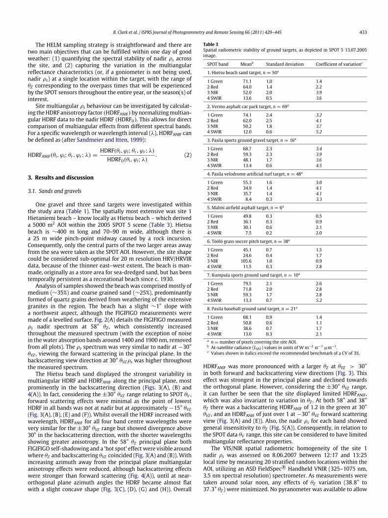
Fig. 4. (A) Site 1 Hietsu beach medium sand SPOT green band multiangular HDRF anisotropy factor (HDRFANIF); mean θZ = 51°. (B) Site 3 Pasila sports ground very finegravel SPOT green band HDRFANIF; mean θZ = 60°.

Fig. 5. (A) General invariance of Hietsu beach medium sand nadir ρs to changes in θZ , as measured on 17.07.2006, 09:40 to 13:40 local time. Solid lines show fitted linearmodels. (B) Hietsu beach medium sand spectral and spatial homogeneity assessed as the average nadir ρs (% HCRF) of 20 stratified random sample sites measured on08.06.2007, 38.8°–37.3° θZ . SD = standard deviation; CV = coefficient of variation.

it should be absorbed before it is reflected back toward themacroscopic surface. Thus, volumetric scattering should increasewith decreasing grain size (Leu, 1977).

For sands and gravels, at a macro-level when the particles areopaque and large compared to wavelength, shadows are cast onneighbouring particles. The observed distribution of shadows onthe surface depends on the specific viewing-illumination geometryand a given sensor’s GIFOV. When viewing and illuminationdirection coincide, all shadows are hidden by the particles thatcast them and local reflectance peaks to give a hot spot (Liang,2004). Coherent backscattering may also contribute to the hotspot effect (Hapke et al., 1996). Surface roughness will meanthat forward scattering viewing will lead to lower reflectancecaused by the backshadow effect (Sandmeier et al., 1998b) ofviewing shadowed surfaces. However, minimum reflectance isnot at maximum forward scattering θVZ because the gap effect(Sandmeier et al., 1998b) means forward scattering viewing θVZnearer to nadir will view deeper into the shadowed gaps betweenparticles. Furthermore, some of the more translucent mineralparticles may transmit some radiation, reducing the impact of thebackshadow effect. Viewing in the backscattering direction willgive higher reflectance, as there are less exposed shadows andmore directly illuminated surfaces. Increased surface roughnessleads to increased non-Lambertian reflectance characteristics(Jackson et al., 1990).

Considering very high θZ where HDRFANIF is likely to be morepronounced, sites 3, 7 and 8 all displayed similar overall HDRFANIFto the Hietsu beach sand (Fig. 6). For reasons discussed above,backscattering in the principal plane was strong with a clearhot spot, whilst forward scattering was minimal, particularly forsite 7 where minimum ρs was at −30° θVZ and ρs was onlyequivalent to nadir ρs at −50° θVZ . For the sands and gravel,HDRFANIF was reduced with increasing azimuth away from theprincipal plane (Fig. 4). Sites 7 and 8 displayed very strong principalplane backscattering over 30° θVZ and at the hot spot. There were,however, some differences with the site 1 medium sand. Givenmineral composition was similar between sites 1, 3 and 7, site 1

had a higher nadir ρs spectrum because of increased volumetricscattering due to the smaller overall grain size (Fig. 2(A)–(C)). Site8, however, had a differentmaterial composition and consequentlyhad a very different ρs spectrum, which was lower and virtuallyflat over the VIS/NIRwavelengths (Fig. 2(D)). Because of the overallgreater surface roughness of sites 3, 7 and 8 compared to site 1, dueto the coarser grain size, HDRFANIF was increased compared to thebeach sand (Figs. 2, 3 and 6). Site 1 sand backscattering at 30° θVZwas slightly less than for the other sites, for example, and also thehot spot HDRFANIF was less.

Within the ±30° θVZ range relating to the SPOT θV , therefore,it can be seen that all the sand and gravel sites displayed limitedHDRFANIF. In terms of desirable HELM calibration target properties,then, as well as the need for a spatially large site, a well-sorted andfiner grainedmaterial is preferable because it will have less surfaceroughness, and consequently less sensitivity to variations in θZ andθVZ . Further, it is also likely to have increased volumetric scatteringleading to a brighter spectrum, useful in better determining HELMcorrection lines.

3.2. Asphalts

Because of their common occurrence globally, asphalts hold in-terest as potential EL calibration targets, and are often suggestedas such. Asphalt surfaces consist of locally sourced crushed aggre-gates of a certain size and shape specification held together witha binding material, usually formed from bitumen. This bitumen orasphalt mix has a complex variable chemical composition, but isessentially formed of hydrocarbons with sulphur and some tracemetals (Herold and Roberts, 2005).

Two sites within the Helsinki metropolitan regionwere studied(Table 1): Firstly, site 2, a car park at the Vermo horse racingstadium, which derived an AOI of 6900 m2 in the 2005 SPOTscene (Table 3); and secondly, site 5 a specific patch of asphalthard-standing within Malmi airfield (6 pixels AOI). Whilst, ingeneral, asphalts displayed a similar limited range in HDRFANIF


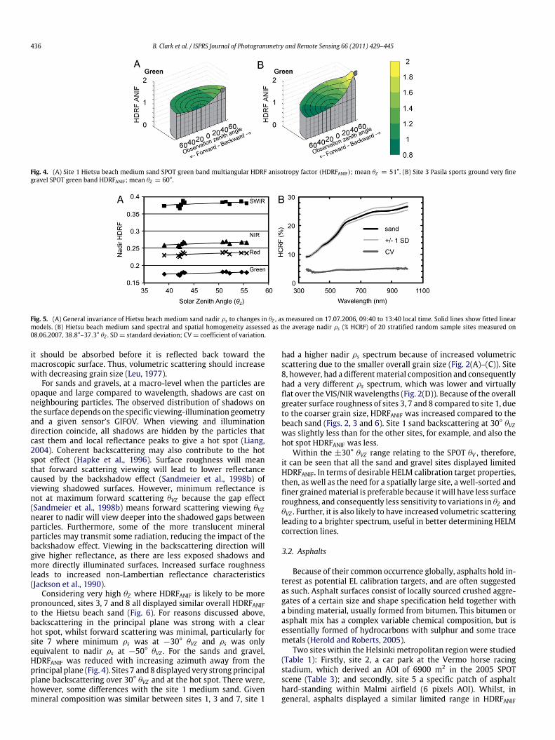
Fig. 6. Multiangular HDRF characteristics of sand and gravel sites: site 3 very fine gravel multiangular principal plane HDRFANIF (A) and principal plane HDRF (B) at 62° θZ ;site 7 very coarse sand principal plane HDRFANIF (C) and principal plane HDRF (D) at 66° θZ ; site 8 very coarse sand principal plane HDRFANIF (E) and principal plane HDRF(F) at 66° θZ .

to the measured sands within the ±30° θVZ range (Fig. 10),asphalt reflectance properties were, however, in every otherway drastically more variable. This is because asphalt reflectancecharacteristics are very sensitive to weathering and ageingprocesses, and consequently change substantially over time.

Within site 2 at the time of measurement in summer 2005,there were three distinct surface areas relating to asphalt age(Fig. 7). Themajority of the site was formed from the oldest asphaltsurface, referred to as sub-site II, which was over 10 years in age.A further significant area, referred to as sub-site I, represented apartial resurfacing that took place ∼5 years before measurement.Furthermore, there were several smaller sections of recent patchrepairs in areas of water ingression damage, the largest of whichwas referred to as sub-site III. This represented an area ∼1 yearold at the time of measurement.

The sub-site III new asphalt surface was totally sealed with acovering of bitumen mix, with no aggregates exposed (Fig. 8(B)).Because of the high absorption properties of the mix, especiallyat shorter wavelengths, the nadir ρs spectrum was very lowand linearly increased only very slightly from a minimum in theUV (0.04 ρs) through to longer wavelengths (0.08ρs) (Fig. 9(B)).The −30°θVZ forward scattering spectrum had a higher ρsat all wavelengths. Hydrocarbon compounds exhibit electronictransitions arising from the excitation of bonding electrons inthe UV and visible, causing this strong absorption (Herold and

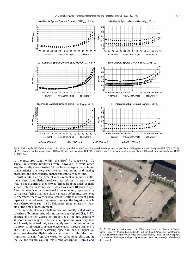
Fig. 7. Vermo car park asphalt year 2005 homogeneity, as shown in GoogleEarthTM imagery:©DigitalGlobe 2005. (A) Sub-site II with ‘‘moderate’’ weathering,(B) sub-site I with ‘‘light’’ weathering, and (C) sub-site III, an area of ‘‘new’’ asphalt.The presence of white painted parking bay lines (10 cm in diameter) can be clearlydetermined.


Fig. 8. Asphalt surfaces (Note: measurement rule scale for (A), (B) and (D) is mm; scale for (C) is cm). Nadir view of (A) site 2 Vermo car park sub-site II ‘‘moderately’’weathered asphalt (>10 years old), (B) site 2 Vermo car park sub-site III newly laid asphalt (∼1 year old), (C) site 5 Malmi airfield hard-standing asphalt (2–3 years old), and(D) site 2 Vermo car park sub-site I ‘‘lightly’’ weathered asphalt (≥5 years old).

Fig. 9. Asphalt spectrums. Solar principal plane nadir view, forward scattering−30° θVZ view, and backscattering 30° θVZ view ρs spectrums, at (A) Vermo car parksub-site II moderately weathered asphalt at 48° θZ ; (B) Vermo car park sub-site IIInew asphalt at 44° θZ ; (C) Malmi airfield hard-standing lightly weathered asphaltat 39° θZ ; and (D) comparison of asphalt nadir spectrums at site 2 Vermo car park:sub-site III ‘‘new’’ asphalt at 44° θZ , ‘‘light’’ weathering of asphalt at sub-site I at 40°θZ , ‘‘moderate’’ weathering of asphalt at sub-site II at 48° θZ .

Roberts, 2005). Further, because the surface had beenmechanicallycompacted it is very flat when new, and this smoothness gaverise to strong forward scattering in the principal plane (Fig. 10(C)),which reached nearly 2.4 times greater than nadir. Therewas also ahot spot, but thiswas a lesser effect. The concentration of scatteringin these two directions contributed to lower reflectance aroundnadir.

Weathering of the asphalt surface had a very strong effect onits spectral properties, giving significant brightening throughoutthe spectrum as the aggregate constituents began to be exposedthrough erosion of the seal, and the amount of surface cover of mixwas reduced (Figs. 8(A), (B), (D) and 9(D)). Furthermore, ageing ofthemix itself led to a loss of complex hydrocarbons and a reductionin the absorption properties, giving a consequent brightening. Asnoted by Herold et al. (2004), this ageing process is caused byphotochemical reactions with sunlight, chemical reactions withatmospheric oxygen, and the influence of heating and cooling.

This leads to three major effects: loss of oily components throughabsorption or volatility, changes in composition through oxidation,and molecular structuring that changes the viscosity of the mix,known as steric hardening. Whilst loss of oily components is arelatively short-term process, the others are more long-term. Anoverall effect is to make the asphalt more prone to structuraldamage through mechanical wear.

After ∼5 years of weathering at sub-site I the aggregates hadbecome partially exposed and the mix itself had become muchbrighter (Figs. 8(D) and 9(D)). Consequently, the sub-site I ρsspectrum was significantly higher, especially in the NIR and SWIRwhere brightening was >10% reflectance, leading to curve thatwas steeper in the visible, but was otherwise a similar slopeto the new asphalt. This represents the intermediate conditionsof light weathering, where the spectrum is determined both byhydrocarbon absorption features, which dominate the spectrumof new asphalt, and by the brighter mineral signals from exposedaggregates. The effects of ageing occur quicker in the early stagesof the process. For example, Herold and Roberts (2005) found thatthe spectral differences between a 1 and 3 year old asphalt surfacewere approximately equivalent to those of a 3 and 10 year oldasphalt, although the structural damage through vehicular usagewas significantly greater for the older asphalt. This brings up theimportant point to note that site 2 is exceptional as a car park asit is only used once or twice a week and is nearly always devoid ofvehicles. This would not be the case for car parks in general, whichcould reasonably be expected to be in constant usage.

The consequence of very low traffic levels at site 2 isthat there is minimal structural damage caused by mechanicalstresses on the asphalt surface. As noted by Herold and Roberts(2005), the most common result of mechanical distressing ofasphalt is cracking, although rutting and ravelling (progressiveasphalt disintegration from the surface downward due to thedislodgement of aggregate particles) may also be present in hightraffic areas. Structural damage decreases brightness, but enhancesmultiangular HDRFANIF, because it increases surface roughnesscausing shadowing, as do the cracks themselves. Furthermore,the exposed asphalt within the cracks is not weathered and thushas the high absorption properties of new asphalt. For heavilytrafficked areas, therefore, an asphalt of equivalent age to Vermosite II would be expected to exhibit a darker spectrum andincreased HDRFANIF because of likely greater structural damage.


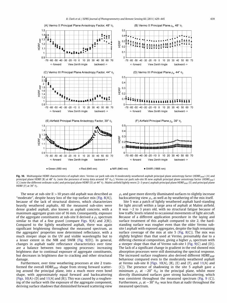
Fig. 10. Multiangular HDRF characteristics of asphalt sites: Vermo car park sub-site II moderately weathered asphalt principal plane anisotropy factor (HDRFANIF) (A) andprincipal plane HDRF (B) at 48° θZ (note the presence of noisy data around 10° θVZ ); Vermo car park sub-site III new asphalt principal plane anisotropy factor (HDRFANIF)(C) (note the different ordinate scale) and principal plane HDRF (D) at 44° θZ ; Malmi airfield lightly worn (2–3 years) asphalt principal plane HDRFANIF (E) and principal planeHDRF (F) at 39° θZ .

The wear at sub-site II >10 years old asphalt was described as‘‘moderate’’, despite heavy loss of the top surface mix (Fig. 8(A)),because of the lack of structural distress, which characterizesheavily weathered asphalts. All the measured sub-sites weredense graded asphalt, also known as asphalt concrete, with amaximum aggregate grain size of 16 mm. Consequently, exposureof the aggregate constituents at sub-site II derived a ρs spectrumsimilar to that of a fine gravel (compare Figs. 9(A) and 2(B)).Compared to the lightly weathered asphalt, there was againsignificant brightening throughout the measured spectrum, asthe aggregates’ properties now determined reflectance, with amuch steeper slope in the UV and visible wavelengths but toa lesser extent in the NIR and SWIR (Fig. 9(D)). In general,changes in asphalt nadir reflectance characteristics over timeare a balance between two opposing processes: increasingbrightness due to continual exposure of aggregate constituents,but decreases in brightness due to cracking and other structuraldamage.

Furthermore, over time weathering processes at site 2 trans-formed the overall HDRFANIF shape from strong forward scatter-ing around the principal plane, into a much more even bowlshape, with approximately equal forward and backscattering(Figs. 10(A)–(D) and 11(A) and (B)). This was caused by a roughen-ing of the surface with the exposure of the aggregate component,deriving surface shadows that diminished forward scattering view

ρs and gave more directly illuminated surfaces to slightly increasebackscattering view ρs, as well as by weathering of the mix itself.

Site 5 was a patch of lightly weathered asphalt hard-standingfor light aircraft within a large area of asphalt at Malmi airfield.It was ∼2 to 3 years old, with no structural fatigue because oflow traffic levels related to occasional movements of light aircraft.Because of a different application procedure in the laying andsurface treatment of this asphalt compared to site 2, the hard-standing surface was rougher even than the older Vermo sub-site I asphalt with exposed aggregates, despite the high remainingsurface coverage of the mix at site 5 (Fig. 8(C)). The mix wasslightly brighter than that used at Vermo, presumably due to adiffering chemical composition, giving a higher ρs spectrum witha steeper slope than that of Vermo sub-site I (Fig. 9(C) and (D)).The lack of a significant change in gradient in the red showed mixabsorption processes were still dominating the spectral response.The increased surface roughness also derived different HDRFANIFbehaviour compared even to the moderately weathered asphaltat Vermo sub-site II (Figs. 10(A), (B), (E) and (F), and 11(A) and(C)). The presence of shadowing in the site 5 asphalt gave aminimum ρs at −20° θVZ in the principal plane, whilst moredirectly illuminated surfaces gave strong backscattering, whichwas consistent throughout the measured spectrum (Fig. 9 (C)).Furthermore, ρs at −30° θVZ was less than at nadir throughout themeasured spectrum.


Fig. 11. (A) Vermo car park sub-site II moderately weathered asphalt SPOT green band multiangular HDRFANIF; mean θZ = 48°. (B) Vermo car park sub-site III new asphaltSPOT green bandmultiangularHDRFANIF;mean θZ = 45°. (C)Malmi airfield hard-standing lightlyweathered asphalt SPOT green bandmultiangularHDRFANIF;mean θZ = 41°.

These measurements clearly show that, as was noted byPuttonen et al. (2009), asphalt surfaces cannot be utilized asstable reflectance targets for EL calibration without detailedknowledge about the surface. New asphalt is too spectrally darkto be a calibration target. Over periods of ∼1 year or more,especially after asphalt has been newly laid, significant changesin brightness and HDRFANIF can be expected. This invalidates anyassumptions of long-term temporal stability, and utilization forEL calibration should only be undertaken for measurements madenear to SPOT image acquisition (<1 year), and with caution.Furthermore, spatial spectral homogeneity cannot be expectedbecause of surface age differences and patch repairs, as well as thepresence of painted lines (Fig. 7), surface contaminants such as oil,and, seemingly obvious, vehicles themselves (Milton et al., 1997).The reflectance of all surface features will be integrated into theGIFOV recorded by the SPOT sensors. In the 2005 image, althoughconvolving the spectral effect of the painted lines to some extent,site 2 derived an average spatial CV of 3.2% in the green, 4.1% in thered, 3.7% in the NIR, and 5.2% in the SWIR (Table 3). Overall thiswasthe highest of all the measured sites of all surface types.

3.3. Artificial and real grass turf

Site 4 was an American football pitch artificial turf surface(Table 1), deriving an AOI of 4800 m2 (Table 3). The turf surfaceconsisted of silicone lubricated polyethylene synthetic grass fibresattached to a rubberized base. Whilst the individual blades were∼50 mm long, the height of turf was ∼30 mm due to the curlinessof the artificial grass fibres and the densely packed nature of the‘canopy’. This lead to a very tightly packed ‘canopy’ top, with aplanophile type structure hiding the gaps beneath and deriving aminimum of shadowing at the surface.

The nadir ρs spectrum increased throughout the visible, witha strong green peak at 565 nm reflecting the colouring of thematerial, and a more level response throughout the NIR and SWIR(Fig. 12 (D)). Furthermore, the forward scattering at −30° θVZwas stronger in the SWIR, whilst the backscattering at 30° θVZwas similar to nadir ρs throughout the measured spectrum. Thiswas also the case considering the whole measured range of θVZ ,

as in the principal plane the surface predominantly displayedforward scattering behaviour (Fig. 13(C) and (D)), due to specularreflections on the horizontally orientated synthetic blades of grass.The silicone lubrication covering may also have contributed to thespecular reflections. HDRFANIF was similar for all the SPOT bands(Fig. 13(C)). There was a minor hot spot effect, but within the±30° θVZ range relating to the SPOT θVHDRFANIF was limited anddecreased with increasing azimuth away from the principal plane(Fig. 14(D)).

However, site 4 does not represent a good HELM calibrationtarget because of the presence of a large number of paintedmarkings and lines, which covered a substantial proportion of thetotal surface area. Enough, at least, to cause variability at the scaleof the GIFOV measured by the SPOT sensors, as these paintedareas had much brighter VIS/NIRρs than the artificial turf itself(Fig. 12(D)). Consequently, site 4 spatial spectrally heterogeneitydescribed by the CV was relatively high (Table 3). Furthermore,artificial turf will not be used to cover large areas unless it is for asporting application, and in such circumstances the application ofpaintedmarkings and lines is very likely.Moreover, the occurrenceand distribution of artificial turf sites is currently extremelylimited, especially at the global scale.

Moran et al. (2001) argued that vegetated sites with >90%cover and very high green leaf area index (LAI) could be utilizedas EL calibration targets, and gave an example of irrigatedmature cotton fields. Similarly, Karpouzli and Malthus (2003)used a sports pitch managed turf in EL calibration. Nonetheless,vegetated sites are problematic for HELM because they are likelyto show temporal variability, and also strong ρs variability withθVZ (Sandmeier et al., 1998b). Vegetation reflectance cannot beexpected to be stable over even short periods of time (days)due to phenological developments, varying plant stress, variationsin leaf and underlying soil moisture content, changes in canopyarchitecture, and differences between species (Pinter et al., 1990).

The site 6 soccer pitch turf (Table 1) is of interest as it representsthe most stable vegetative conditions that can be expected tooccur: the turf was constantly managed throughout the spring andsummer through watering and mowing of a single planted grassspecies. Aswould be expected, the site 6 nadir ρs spectrum showed


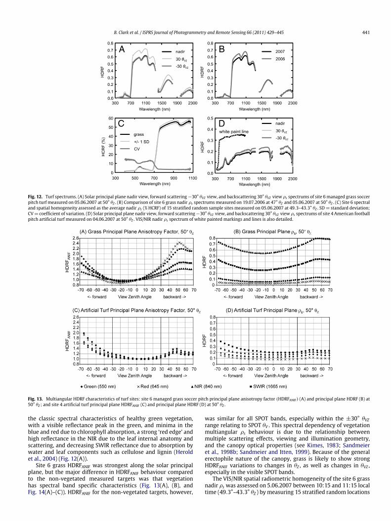
Fig. 12. Turf spectrums. (A) Solar principal plane nadir view, forward scattering−30° θVZ view, and backscattering 30° θVZ view ρs spectrums of site 6managed grass soccerpitch turf measured on 05.06.2007 at 50° θZ . (B) Comparison of site 6 grass nadir ρs spectrums measured on 19.07.2006 at 47° θZ and 05.06.2007 at 50° θZ . (C) Site 6 spectraland spatial homogeneity assessed as the average nadir ρs (% HCRF) of 15 stratified random sample sites measured on 05.06.2007 at 49.3–43.3° θZ . SD = standard deviation;CV= coefficient of variation. (D) Solar principal plane nadir view, forward scattering−30° θVZ view, and backscattering 30° θVZ view ρs spectrums of site 4 American footballpitch artificial turf measured on 04.06.2007 at 50° θZ . VIS/NIR nadir ρs spectrum of white painted markings and lines is also detailed.

Fig. 13. Multiangular HDRF characteristics of turf sites: site 6 managed grass soccer pitch principal plane anisotropy factor (HDRFANIF) (A) and principal plane HDRF (B) at50° θZ ; and site 4 artificial turf principal plane HDRFANIF (C) and principal plane HDRF (D) at 50° θZ .

the classic spectral characteristics of healthy green vegetation,with a visible reflectance peak in the green, and minima in theblue and red due to chlorophyll absorption, a strong ‘red edge’ andhigh reflectance in the NIR due to the leaf internal anatomy andscattering, and decreasing SWIR reflectance due to absorption bywater and leaf components such as cellulose and lignin (Heroldet al., 2004) (Fig. 12(A)).

Site 6 grass HDRFANIF was strongest along the solar principalplane, but the major difference in HDRFANIF behaviour comparedto the non-vegetated measured targets was that vegetationhas spectral band specific characteristics (Fig. 13(A), (B), andFig. 14(A)–(C)). HDRFANIF for the non-vegetated targets, however,

was similar for all SPOT bands, especially within the ±30° θVZrange relating to SPOT θV . This spectral dependency of vegetationmultiangular ρs behaviour is due to the relationship betweenmultiple scattering effects, viewing and illumination geometry,and the canopy optical properties (see Kimes, 1983; Sandmeieret al., 1998b; Sandmeier and Itten, 1999). Because of the generalerectophile nature of the canopy, grass is likely to show strongHDRFANIF variations to changes in θZ , as well as changes in θVZ ,especially in the visible SPOT bands.

The VIS/NIR spatial radiometric homogeneity of the site 6 grassnadir ρs was assessed on 5.06.2007 between 10:15 and 11:15 localtime (49.3°–43.3° θZ ) by measuring 15 stratified random locations


Fig. 14. Site 6 managed grass soccer pitch SPOT (A) green band, (B) red band, and (C) NIR band HDRFANIF; mean θZ = 44°. (D) Site 4 artificial turf SPOT red band HDRFANIF;θZ = 44°.

using the same measurement approach as applied to site 1. Thisderived consistently small SD, but the very low ρs of the grass inthe visible wavelengths derived high CVs (Fig. 12(C)). Further, atthe scale of the SPOT GIFOV, the site 6 grass derived low averagespatial CVs (Table 3). Overall, then, as a consequence of its carefulmanagement, site 6 was very spectrally homogeneous consideringit was a vegetative target.

Furthermore, the temporal spectral stability of site 6 wasassessed by measuring the grass ρs nadir spectrum on 19.07.2006at 47° θZ and on 05.06.2007 at 50° θZ . Comparison showedan average absolute difference (ρs %) of 0.4% in the visible,5.2% in the NIR, and 3.6% for the 1000–1340 nm SWIR, andwith a small variation similar to the visible for the SWIR from1440–1780 nm and 1980–2300 nm (Fig. 12(B)). This indicatedsite 6 grass was actually relatively stable over time, although NIRand SWIR temporal variation exceeded the desired 0.02ρs limit.Nevertheless, the very low reflectance of vegetation in the visiblespectrum, and its spectral band specific HDRFANIF behaviour,makesit unsuitable for use in SPOT data EL calibration.

3.4. HELM-1 nadir calibration error estimates

Given the stated ±0.02ρs VIS/NIR benchmark for successfulatmospheric correction, HELM-1 nadir calibration uncertainty alsoneeds to be within this range. The actual error encountered willdepend on the multiangular ρs characteristics of the utilizedsurface and the SPOT image geometry. Taking site 1 as themost appropriate HELM calibration target, the difference betweenmultiangular and nadir ρs within the ±30° θVZ range relating tothe SPOT θV was minimal in the forward scattering view direction,but >0.02 in the backscattering view along the principal plane(Table 5).

Examination of the site 1 data determined the backscatteringθVZ in the principal plane at which the 0.02 calibration limit wasexceeded occurred at approximately ≥ 20° θVZ . Consideration wasalso given to the azimuthal distribution of the difference in ρsbetween nadir and backscattering in the 30° θVZ and 20° θVZ range;given differences in the forward scattering were minimal. At site 1the linear modelled data for 30° θVZ from nadir ρs fell below 0.02in all spectral bands by 55° azimuth from the principal plane. At20° θVZ , backscattering variation from nadir ρs in all spectral bandswas below 0.02 apart from a few degrees from the principal plane.

Fig. 15. Generalized error model for the application of HELM-1 nadir calibrationto SPOT imagery with a possible ±30° range in view incidence angles (θV ). Asillustrated in grey shading, the difference between nadir ρs and angular ρs mayexceed 0.02 at backscatter viewing θV ≥ 20° within ±55° azimuth of the solarprincipal plane, assuming azimuthal symmetry in the target multiangularcharacteristics. Because of the SPOT satellites’ orbit geometry, imagery viewing thebackscatteringwill always be denoted in themetadata byR (right, negative, east) θV .

Based on site 1, therefore, a generalized errormodel for HELM-1calibration to nadirρs for SPOT imagery using an appropriate targetis ≤ 2% (0.02) ρs across all bands. As illustrated in Fig. 15, the ex-ception is when θV is≥ R20° in the backscattering directionwithin±55° azimuth of the solar principal plane, assuming azimuthalsymmetry in calibration target multiangular ρs behaviour. SPOTimagery with viewing geometry falling within these limits couldbe HELM-1 atmospherically corrected, but error in the calibrationmay then exceed 0.02ρs and, based on site 1, could be >0.04 ρsat maximum backscattering viewing θV in or near to the principalplane (Table 5). Alternatively, it is possible simply to avoid utilizingsuch scenes by establishing illumination and view geometries be-fore ordering. These HELM-1 limitations demonstrate that, if at allpossible, multiangular ρs measurements of the calibration target(at least along the principal plane in the backscattering direction)should be collected and are useful information. Estimates of thecalibration error in applying HELM-1 to the SPOT imagery datasetweremade based on themodelled geometric ρs derived for the site1 medium sand. The overall average calibration RMSE for all bandsand all years was 0.014 ρs and, except for the 2002 image, bandspecific angular ρs was always greater than the nadir ρs; i.e. nadircalibration was always an underestimation (Table 6).

4. Conclusions

In this study, calibration site selection requirements forHELM atmospheric correction of SPOT HRV/HRVIR/HRG data were


Table 5Variation in ρs measured at site 1 in the solar principal plane and orthogonal plane at ±30° sensor view zenith angle (θVZ ) relative to nadir for all SPOT bands.

Hietsu beach Medium Sand Spectral bandNadir ρs

−30°θVZFSa

30°θVZBSa

DifferencebFSa

DifferencebBSa

RelativecDiff BS (%)

17.07.2006 1 Green: 0.180 0.186 0.216 0.006 0.036 20.0θZ = 55° 2 Red: 0.236 0.244 0.278 0.008 0.042 17.8Principal plane 3 NIR: 0.266 0.277 0.307 0.011 0.042 15.8

4 SWIR: 0.380 0.399 0.423 0.019 0.043 10.8Av. all bands 0.011 0.041

17.07.2006 1 Green: 0.182 0.186 0.190 0.004 0.008 4.4θZ = 51.4° 2 Red: 0.240 0.244 0.251 0.005 0.012 5.0Orthogonal plane 3 NIR: 0.270 0.275 0.282 0.006 0.013 4.8

4 SWIR: 0.385 0.396 0.401 0.010 0.016 4.0Av. all bands 0.006 0.012

All measurements are HDRF rounded to the nearest 10th of a percent.a FS = Forward Scattering view; BS = Backscattering view.b Difference in HDRF with nadir measurements.c Relative difference (%) in the backscattering direction with nadir HDRF.

Table 6Estimates of HELM-1 nadir calibration errors for the SPOT imagery dataset using site 1, Hietsu beach sand, as a calibration target.

Dataset 1Image information

Spectral band Nadir ρsa Geometric ρs

b Error in HELM calibration

1993 1 Green 0.171 0.172 −0.001θV Left 9.3°; θZ = 38.2° 2 Red 0.220 0.221 −0.001ϕr299.1° 3 NIR 0.247 0.249 −0.002ϕrpp

c 60.9° FS RMSE all bands 0.001

1994 1 Green 0.173 0.184 −0.011θV Left 29.7°; θZ = 43.5° 2 Red 0.227 0.241 −0.014ϕr291.7° 3 NIR 0.254 0.269 −0.015ϕrpp

c 68.3° FS RMSE all bands 0.013

2002 1 Green 0.177 0.176 0.001θV Left 2.5°; θZ = 37.5° 2 Red 0.222 0.222 0.000ϕr298.2° 3 NIR 0.248 0.248 0.000ϕrpp

c 61.8° FS 4 SWIR 0.350 0.351 −0.001RMSE all bands 0.001

2003 1 Green 0.176 0.195 −0.019θV Right 28.7°; θZ = 43.8° 2 Red 0.229 0.252 −0.023ϕr121.6° 3 NIR 0.256 0.279 −0.023ϕrpp

c 58.4° BS 4 SWIR 0.361 0.390 −0.029RMSE all bands 0.024

2005 1 Green 0.171 0.181 −0.010θV Right 16.1°; θZ = 39.2° 2 Red 0.225 0.237 −0.012ϕr125.2° 3 NIR 0.247 0.259 −0.012ϕrpp

c 54.8° BS 4 SWIR 0.353 0.368 −0.015RMSE all bands 0.012

RMSE 1 Green RMSE for all years 0.0112 Red RMSE for all years 0.0133 NIR RMSE for all years 0.0134 SWIR RMSE for all years 0.019Average RMSE for all bands and all years 0.014Green RMSE for Forward Scattering only 0.006Red RMSE for Forward Scattering only 0.008NIR RMSE for Forward Scattering only 0.009SWIR error for Forward Scattering (2002) only −0.001Average RMSE for Forward Scattering all bands and all years (1993, 1994, 2002) 0.008Green RMSE for Backscattering only 0.015Red RMSE for Backscattering only 0.018NIR RMSE for Backscattering only 0.018SWIR RMSE for Backscattering only 0.023Average RMSE for Backscattering all bands and all years (2003 and 2005) 0.019

a The nadir ρs (HDRF) of the calibration target is the value used to calibrate the HELM-1 correction model.b The geometric ρs of the calibration target is the ρs corresponding to the view and illumination conditions at the time of scene capture, and estimated from BRDF models

fitted to the goniometer field measurements.c ϕrpp is the smallest azimuth angle between the sensor azimuth and the solar principal plane; FS is a sensor view of the forward scattering, BS is a sensor view of the

backscattering.

discussed and the physical mechanisms behind the varyingreflectance characteristics of the measured surfaces were consid-ered. Results showed all surfaces exhibited some degree of non-Lambertian multiangular reflectance behaviour within the SPOTsensors’ ±31° θVZ range, particularly along the solar principal

plane, as well as spatial and temporal spectral variability. Ideally,therefore, the multiangular reflectance characteristics of a calibra-tion target should be captured. Of the sands, gravel, asphalts andturf surface types investigated, medium grained sand offered themost appropriate characteristics. The sandwas themost spectrally


stable site over time, as weathering changes are a long-term pro-cess. Themost desirable sand properties are awell-sorted and finergrained material because this has less surface roughness, and con-sequently less sensitivity to θZ and θVZ variations, and lesser mul-tiangular ρs anisotropy. Further, it is also likely to have increasedvolumetric scattering leading to a brighter spectrum, useful in bet-ter determining empirical lines.

Results from a grass turf showed vegetation has too strongwavelength dependent multiangular ρs properties, and is toospectrally dark in the visible bands, to be a viable HELM calibrationtarget; even if heavily managed sites may actually be relativelyspatially and temporally spectrally stable. Use of artificial turfas a calibration target is problematic because of very limitedoccurrence and the usual presence of a large number of paintedmarkings for sporting applications. Asphalts are often suggestedas suitable vegetation-free calibration targets. However, this studyclearly showed general usage is not recommendable withoutdetailed knowledge of a specific site’s characteristics and theavailability of field measurements made very near to the imageryacquisition time. New asphalt is too spectrally dark to be acalibration target, but weathers quickly so that within the spaceof a few years the ρs spectrum resembles that of the exposedconstituent gravel aggregates. The presence of structural damagefrom usage will further increase multiangular ρs anisotropy,because of a consequent significant increase in surface rougheningand shadowing. As well as temporal variance, asphalt use canbe problematic because of the presence of patch repairs, paintedmarkings, and motor vehicles, which all increase spatial spectralheterogeneity.

Where angular ρs field measurements are unavailable, ELcalibrations to nadir ρs for SPOT imagery with viewing geometriesnear to the solar principal plane are likely to derive significanterror, as here multiangular ρs variations will be greatest. In allcases, field measurements should be made within the θZ rangewithinwhich SPOT overpasswill occur, and it is recommended thatdetailed knowledge and measurements of the calibration site becollected and a minimum of assumptions be made. The findingsof this study are also generally applicable to EL atmosphericcorrection of any other medium or high resolution optical satellitedata. Theywill, therefore, offer assistance toworkers in identifyingsuitable EL calibration sites and help in the optimization of effortsin the time consuming and costly process of measuring ρs in thefield.

Acknowledgements

This study forms part of the Academy of Finland fundedTAITA and TAITATOO projects, conducted at the Department ofGeosciences and Geography of the University of Helsinki. The SPOTdata was provided by Spot Image under OASIS research grant 51.The authors are grateful to AlemuGonsamoGosa for his commentson the text, and to Teemu Hakala, Janne Heiskanen, Eetu Puttonen,andMika Siljander for their assistance in the collection of field data.Three anonymous reviewers are thanked for their constructivecomments on the original version of this manuscript.

References

Anderson, K., Milton, E.J., 2006. On the temporal stability of ground calibrationtargets: implications for the reproducibility of remote sensing methodologies.International Journal of Remote Sensing 27 (16), 3365–3374.

Bannari, A., Omari, K., Teillet, P.M., Fedosejevs, G., 2005. Potential of getis statisticsto characterize the radiometric uniformity and stability of test sites used for thecalibration of earth observation sensors. IEEE Transactions on Geoscience andRemote Sensing 43 (12), 2918–2925.

Chavez Jr., P.S., 1996. Image-based atmospheric corrections—revisited and im-proved. Photogrammetric Engineering & Remote Sensing 62 (9), 1025–1036.

Clark, B.J.F., 2010. Enhanced processing of SPOT multispectral satellite im-agery for environmental monitoring and modelling. Ph.D. Thesis, De-partment of Geosciences and Geography. University of Helsinki. Finland.http://urn.fi/URN:ISBN:978-952-10-6306-0 (accessed 08.02.11).

Clark, B.J.F., Pellikka, P.K.E., 2009. Landscape analysis usingmultiscale segmentationand object orientated classification. In: Röder, A., Hill, J. (Eds.), Recent Advancesin Remote Sensing and Geoinformation Processing for Land DegradationAssessment. Taylor & Francis, London, pp. 323–341.

Clark, B., Suomalainen, J., Pellikka, P., 2011. An historical empirical line method forthe retrieval of surface reflectance factor frommulti-temporal SPOTHRV,HRVIRand HRG multispectral satellite imagery. International Journal of Applied EarthObservation and Geoinformation 13 (2), 292–307.

Clark, B., Suomalainen, J., Pellikka, P., 2010. A comparison of methods for theretrieval of surface reflectance factor from multi-temporal SPOT HRV, HRVIRand HRG multispectral satellite imagery. Canadian Journal of Remote Sensing36 (4), 397–411.

de Vries, C., Danaher, T., Scarth, P., Phinn, S., 2007. An operational radiometriccalibration procedure for the Landsat sensors based on pseudo-invariant targetsites. Remote Sensing of Environment 107 (3), 414–429.

Gellman, D.I., Biggar, S.F., Dinguirard, M.C., Henry, P.J., Moran, M.S., Thome, K.J.,Slater, P.N., 1993. Review of SPOT-1 and -2 calibrations at white sands fromlaunch to the present. Proceedings of SPIE 1938 (13), 118–125.

Hapke, B., 1993. Theory of Reflectance and Emittance Spectroscopy. CambridgeUniversity Press, Cambridge, UK.

Hapke, B., Dominick, D., Nelson, R., Smythe, W., 1996. The cause of the hot spot invegetation canopies and soils: shadow-hiding versus coherent backscattering.Remote Sensing of Environment 58 (1), 63–68.

Herold, M., Roberts, D., 2005. Spectral characteristics of asphalt road aging anddeterioration: implications for remote-sensing applications. Applied Optics 44(20), 4327–4334.

Herold, M., Roberts, D., Gardner, M.E., Dennison, P.E., 2004. Spectrometry for urbanarea remote sensing—development and analysis of a spectral library from 350to 2400 nm. Remote Sensing of Environment 91 (3–4), 304–319.

Jackson, R.D., Teillet, P.M., Slater, P.N., Fedesojevs, G., Jasinski, M.F., Aase, J.K.,Moran, M.S., 1990. Bidirectional measurements of surface reflectance for viewangle corrections of oblique imagery. Remote Sensing of Environment 32 (2–3),189–202.

Karpouzli, E., Malthus, T., 2003. The empirical line method for the atmosphericcorrection of IKONOS imagery. International Journal of Remote Sensing 20 (13),2653–2662.

Kimes, D.S., 1983. Dynamics of directional reflectance factor distributions forvegetation canopies. Applied Optics 22 (9), 1364–1372.

Leu, D., 1977. Visible and near-infrared reflectance of beach sands: a study on thespectral reflectance/grain size relationship. Remote Sensing of Environment 6(3), 169–182.

Liang, S., 2004. Quantitative Remote Sensing of Land Surfaces. John Wiley & SonsInc., New Jersey.

Milton, E.J., Lawless, K.P., Roberts, A., Franklin, S.E., 1997. The effects of unresolvedscene elements on the spectral response of calibration targets: an example.Canadian Journal of Remote Sensing 23 (3), 252–256.

Moran, M.S., Bryant, R., Thome, K., Ni, W., Nouvellon, Y., Gonzalez-Dugo, M.P., Qi,J., Clarke, T.R., 2003. A refined empirical line approach for reflectance retrievalfrom Landsat-5 and Landsat-7 ETM+. IEEE Transactions on Geoscience andRemote Sensing 41 (6), 1411–1414.

Moran, M.S., Bryant, R., Thome, K., Ni, W., Nouvellon, Y., Gonzalez-Dugo, M.P., Qi,J., Clarke, T.R., 2001. A refined empirical line approach for reflectance retrievalfrom Landsat-5 and Landsat-7 ETM+. Remote Sensing of Environment 78 (1–2),71–82.

Moran, M.S., Jackson, R.D., Slater, P.N., Teillet, P.M., 1992. Evaluation of simplifiedprocedures for retrieval of land surface reflectance factors from satellite sensoroutput. Remote Sensing of Environment 41 (2–3), 169–184.

Moran, M.S., Jackson, R.D., Hart, G.F., Slater, P.N., Bartell, R.J., Biggar, S.F., Gellman,D.I., Santer, R.P., 1990. Obtaining surface reflectance factors from atmosphericand view angle corrected SPOT-1 HRV data. Remote Sensing of Environment 32(2–3), 203–214.

Pinter, P.J., Jackson, R.D., Moran, S.M., 1990. Bidirectional reflectance factors ofagricultural targets: a comparison of ground-, aircraft-, and satellite-basedobservations. Remote Sensing of Environment 32 (2–3), 215–228.

Puttonen, E., Suomalainen, J., Hakala, T., Peltoniemi, J.I., 2009. Measurement ofreflectance properties of asphalt surfaces and their usability as reference targetsfor aerial photos. IEEE Transactions on Geoscience and Remote Sensing 47 (7),2330–2339.

Rondeaux, G., Steven, M.D., Clark, J.A., Mackay, G., 1998. La Crau; a European testsite for remote sensing validation. International Journal of Remote Sensing 19(14), 2775–2788.

Sandmeier, S.R., Itten, K.I., 1999. A field goniometer system (FIGOS) for acquisition ofhyperspectral BRDF data. IEEE Transactions on Geoscience and Remote Sensing37 (2), 978–986.

Sandmeier, S., Müller, C., Hosgood, B., Andreoli, G., 1998a. Sensitivity analysis andquality assessment of laboratory BRDF data. Remote Sensing of Environment 64(2), 176–191.

Sandmeier, S., Müller, C., Hosgood, B., Andreoli, G., 1998b. Physical mechanismsin hyperspectral BRDF data of grass and watercress. Remote Sensing ofEnvironment 66 (2), 222–233.

http://urn.fi/URN:ISBN:978-952-10-6306-0


Santer, R., Gu, X.F., Guyot, G., Deuzé, J.L., Devaux, C., Vermote, E., Verbrugghe, M.,1992. SPOT calibration at the La Crau test site (France). Remote Sensing ofEnvironment 41 (2–3), 227–237.

Schroeder, T.A., Cohen, W.B., Song, C., Canty, M.J., Yang, Z., 2006. Radiometriccorrection of multi-temporal landsat data for characterization of earlysuccessional forest patterns inwesternOregon. Remote Sensing of Environment103 (1), 16–26.

Slater, P.N., Biggar, S.F., Holm, R.G., Jackson, R.D., Mao, Y., Moran, M.S., Palmer,J.M., Yuan, B., 1987. Reflectance and radiance-based methods for the in-flightabsolute calibration of multispectral sensors. Remote Sensing of Environment22 (1), 11–37.

Smith, G.M., Milton, E.J., 1999. The use of the empirical line method to calibrateremotely sensed data. International Journal of Remote Sensing 24 (5),1143–1150.

Spot Image Corporation. DIMAP format description. 1997. http://www.spotimage.com/automne_modules_files/standard/public/p555_fileLINKEDFILE1_cap.pdf (accessed 29.01.11).

Suomalainen, J., 2006. Multiangular spectrometry and optical properties ofdebris covered surfaces. M.Sc. Thesis. Department of Physics. Universityof Helsinki. Helsinki, Finland. http://ethesis.helsinki.fi/julkaisut/mat/fysik/pg/suomalainen/ (accessed 08.02.11).

Suomalainen, J., Hakala, T., Peltoniemi, J., Puttonen, E., 2009. Polarisedmultiangularreflectance measurements using the finnish geodetic institute field goniospec-trometer. Sensors 9 (5), 3891–3907.

Teillet, P.M., Fedosejevs, G., Gauthier, R.P., O’Neil, N.T., Thome, K.J., Biggar, S.F.,Ripley, H., Meygret, A., 2001. A generalized approach to the vicarious calibrationofmultiple earth observation sensors using hyperspectral data. Remote Sensingof Environment 77 (3), 304–327.

Thome, K.J., 2001. Absolute radiometric calibration of Landsat 7 ETM+ usingthe reflectance-based method. Remote Sensing of Environment 78 (1–2),27–38.

Thome, K., Markham, B., Barker, J., Slater, P., Biggar, S., 1997. Radiometric calibrationof landsat. Photogrammetric Engineering & Remote Sensing 63 (7), 853–858.

Tso, B., Mather, P.M., 2001. ClassificationMethods for Remotely Sensed Data. Taylor& Francis, London.

Wentworth, C.K., 1922. A scale of grade and class terms for clastic sediments. Journalof Geology 30 (5), 377–392.

Wheeler, R.J., LeCroy, S.R., Whitlock, C.H., Purgold, G.C., Swanson, J.S., 1994. Surfacecharacteristics for the alkali flats and dunes regions at white sands missilerange, New Mexico. Remote Sensing of Environment 48 (2), 181–190.

Xu, J., Huang, J., 2006. Refined empirical line method to calibrate IKONOS imagery.Journal of Zhejiang University Science A 7 (4), 641–646.

http://www.spotimage.com/automne_modules_files/standard/public/p555_fileLINKEDFILE1_cap.pdf













http://ethesis.helsinki.fi/julkaisut/mat/fysik/pg/suomalainen/









the selection of appropriate spectrally bright pseudo-invariant ground targets for use in empirical...

Documents