the scale of geometric texture - drexel ccikon/publication/goxholm_eccv12_geomtext...the scale of...

The Scale of Geometric Texture

Geoffrey Oxholm, Prabin Bariya, and Ko Nishino

Department of Computer ScienceDrexel University, Philadelphia, PA 19104, USA

gao25,pb335,[email protected]

Abstract. The most defining characteristic of texture is its underlying geometry.Although the appearance of texture is as dynamic as its illumination and view-ing conditions, its geometry remains constant. In this work, we study the fun-damental characteristic properties of texture geometry—self similarity and scalevariability—and exploit them to perform surface normal estimation, and geomet-ric texture classification. Textures, whether they are regular or stochastic, exhibitsome form of repetition in their underlying geometry. We use this property toderive a photometric stereo method uniquely tailored to utilize the redundancyin geometric texture. Using basic observations about the scale variability of tex-ture geometry, we derive a compact, rotation invariant, scale-space representationof geometric texture. To evaluate this representation we introduce an extensivenew texture database that contains multiple distances as well as in-plane and out-of plane rotations. The high accuracy of the classification results indicate thedescriptive yet compact nature of our texture representation, and demonstratesthe importance of geometric texture analysis, pointing the way towards improve-ments in appearance modeling and synthesis.

1 Introduction

With important applications in remote sensing, industrial surface inspection, and scenesegmentation, texture analysis has been a popular area of study in computer vision fordecades. Typically, this analysis is done on the 2D appearance of texture. Whereasthe appearance of a texture depends greatly on illumination and viewing conditions,the underlying 3D geometry remains constant. We pursue a deeper understanding oftexture geometry in order to enable important tasks, such as object recognition, to bedone reliably in any condition. To do so, we study the two primary characteristics ofgeometric texture—self similarity and scale variability—and exploit them to performsurface normal estimation and geometric texture recognition.

To demonstrate the importance of texture geometry we first introduce a photometricstereo method specifically derived to leverage the repetitious nature of geometric tex-ture. We observe that the appearance of each point is determined fundamentally by boththe surface orientation at that point, and whether or not it is being directly illuminated.Since each of these factors cannot be estimated without knowledge of the other, wemust estimate them jointly. To do so, we derive a probabilistic graphical formulation inwhich these two conditionally independent factors are linked by their combined effecton the appearance of each point. We sequentially order the dense set of observations as

2 Geoffrey Oxholm, Prabin Bariya, and Ko Nishino

the light is waved over the texture. This allows us to derive novel priors for both factors.In particular, we leverage the similarity of geometry that is present in spatially disjointlocations as a prior on the surface normals. Pixels whose intensities vary similarly asthe light moves must have similar orientations. This increased contextual informationallows us to minimize the effect of self-occlusion and interreflection.

Our second main contribution is a rotation-invariant scale-space representation ofthe geometry of texture. Our aim is to compactly encode how the apparent texture ge-ometry varies with its distance from the observer so that a texture can be identifiedreliably regardless of its distance and orientation. Since the 3D surface geometry it-self cannot be reliably recovered due to discontinuities of the surface, we directly usethe surface normal field recovered with the proposed texture photometric stereo as thefoundation for our representation. We first represent the surface normals using theirspherical coordinates. This allows us to describe the geometry using a 2D histogram inwhich rotations of the texture correspond to shifts along the azimuthal axis. By applyingthe 2D Fourier transform we obtain a rotationally invariant representation of the texturegeometry. Next, we compute the scale space of the texture geometry by convolving thesurface normal field with Gaussian kernels of increasing standard deviations until thesurface normal field is completely coherent. We show that this scale space of geomet-ric texture accurately captures the evolution of the apparent surface normal field overincreasing distance, and as such, approximates the underlying geometric scale space.

Our final contribution is a new texture database consisting of over 40, 000 imagesthat we use to demonstrate the descriptiveness of our scale-space representation. Weperform extensive classification experimentation with query textures at multiple dis-tances, with varying degrees of in-plane and out-of-plane rotations as well as undersimulated noise. In total, we test our representation on 600 combinations of distanceand orientation. The high accuracy of the classification results indicate the descriptiveyet compact nature of our texture representation, and demonstrates the importance ofgeometric texture analysis.

2 Related work

Past work on texture analysis has focused primarily on the 2D imaged appearance oftextures. In this domain, many methods have been proposed for rotation invariant andscale invariant classification [9,12]. Similarly, a number of methods have been proposedfor scale-space analysis of texture appearance [7]. The appearance of texture, however,depends fundamentally on the underlying surface geometry. Unlike its appearance, thegeometry of a texture does not change with the illumination and viewing conditions. Inthis work we focus directly on the geometry of surface texture and derive a rotationallyinvariant scale-space representation which we use to perform classification.

There has been some attention to illumination invariance. Smith [20] use photo-metric stereo to recover surface normals and then encode them as a surface orientationhistogram. This approach, however, is geared at analysis to find surface defects, whereasour method is being used to perform classification. McGunnigle and Chantler [15] andBarsky and Petrou [2] extract and use explicit 3D shape and surface reflectance infor-mation to perform classification. Penirschke et al. [19] propose an illumination invariant

The Scale of Geometric Texture 3

classification scheme based on earlier work by Chantler et al. [6] wherein they studythe effect of changes in illumination direction on the image texture. Other approacheshave involved explicitly training a classifier on multiple images of the texture fromdifferent viewpoints and illumination conditions [13, 22]. Dana and Nayar [8] modeltexture surface as a Gaussian-distributed random height field. To avoid this assump-tion we develop a novel scale-based representation in the frequency domain. Althoughsome authors have considered the effect of the underlying geometry, by studying it di-rectly we deepen the understanding of texture, and enable improvements to appearancemodeling and synthesis.

In order to analyze the scale variability of geometric texture, dense and accuratesurface normal information must be gathered. As first introduced by Woodham [23], thetechnique of photometric stereo enables the extraction of accurate surface orientationsfor simple Lambertian objects. As noted by Nayar et al. [16], problems arise whenself-occlusions cause shadows, or interreflection exaggerates illumination conditions.Although there have been many advances in photometric stereo to these, and other ends,our method tackles the less-studied problem of estimating the geometry of textures.

To address self-occlusions, Barsky and Petrou [3] assume that each pixel is directlyilluminated in at least two images. They then ignore light source directions where theobserved intensity is low. Chandraker et al. [5] model light source visibility using aMarkov Random Field with a strong spatial prior that encourages detection of largeshadows. Similarly, Sunkavalli et al. [21], cluster pixels into “visibility subspaces” byobserving the effect of large shadows. Nayar et al. [17] project a moving pattern ontothe scene to separate the effect of direct illumination from that of interreflection andother “global” illumination phenomena. Wu and Tang [24] collect a dense set of imagesand use their inherent redundancy to detect and discard the observations that are mostimpacted by global illumination. We further exploit redundancy by leveraging the rep-etitious nature of texture. In a manner similar to that of Koppal and Narasimhan [11],we manually wave a light source over the texture and detect similarly oriented sur-face patches in physically separate locations based on the similarity of their appearancevariation. Unlike Koppal and Narasimhan, we use the full appearance profile, not justextrema. This allows us to establish a non-parametric distribution of orientation vectorsthat we use as a prior in our expectation maximization framework.

3 Texture photometric stereo

Textures, whether they are regular or stochastic, exhibit some form of repetition in theirunderlying geometry. We exploit this repetition in our texture photometric stereo inorder to recover accurate surface normals.

3.1 Robust estimation

As light passes over a Lambertian texture the intensity Ixt of a pixel x rises and fallsdepending on the relative angle of the light source direction lt at that time t, and thesurface orientation nx at that point according to the basic Lambertian reflectance model

Ixt = ρxmax(0,nx · lt) , (1)


1

N0

(a) Observed intensities (b) Lighting directions

Fig. 1: Observed intensity profile and corresponding relative lighting direction at a singlepixel. We use the intensity profile of a pixel (a) to estimate its light-source visibility. Shown asthick curves, convex regions of the (smoothed) intensity profile serve as good initial estimates ofwhen a pixel is directly illuminated as they correspond to times when the light source passes nearthe surface normal (b).

(a) Sample (b) Basic error (c) Our error

(d) True (e) Basic (f) Ours

(g) True normals

(h) Basic normals

(i) Our normals

Fig. 2: Synthetic scene ground truth comparison. Without any model of light-source visibility,shadows smooth the recovered normal field (e). Using our method results in an accurate esti-mation (f). Brighter pixels in the error fields of (b) and (c) correspond to greater angular error.In the right half we show a slice of normals between two spheres. Note how the normals be-tween the spheres in the basic method results (h) have been corrupted. Ray tracing interpolationis responsible for slight inconsistencies between our results and the ground truth.

where ρx is the albedo value at that point. Following Koppal and Narasimhan [11],as the light is waved over the texture, we take k discrete observations, and call Ix =Ixt | t = 1, . . . , k the intensity profile of pixel x. Fig. 1 shows the path of the movinglight source on the unit hemisphere centered at a surface point. If we align the northpole of the hemisphere with the surface orientation at that point, then in accordancewith Eq. 1, as the light moves closer to the pole, the observed intensity will increase.

Unfortunately, this model ignores a fundamental factor in appearance—light sourcevisibility. Small scale self-occlusions lead to shadows in small regions and interreflec-tion will increase the observed intensity. As shown in Fig. 2, failure to disregard theseobservations will result in inaccurate estimations of the underlying normal field. In oursynthetic experimentation, our method results in a median error of 2.3, while the tra-ditional method results in a median error of 14.8.


We use a binary visibility function V xt to indicate whether or not pixel x at time t isdirectly illuminated,

V xt =

1 if pixel x is directly illuminated0 otherwise .

(2)

By applying this function to both the observed intensity Ixt , as well as the predictedintensity, we are able to effectively ignore misleading values. This augmented versionof the Lambertian reflectance model may be written as

V xt Ixt = V xt ρ

xnx · lt , (3)

where the max function from Eq. 1 has been absorbed into V . Since the surface normalsare unit vectors, we simplify this notation by representing the albedo-scaled normal asNx = ρxnx, where ρx = ‖Nx‖.

A simple approach to estimating V would be to set V xt = 0 for low intensity ob-

servations. For pixels with low albedo values, however, this is too limiting. A better ap-proach is to use the portions of the light trajectory that are near the normal direction. Asshown in Fig. 1a, we estimate these regions as convex portions of the intensity profile.To account for noise, we first smooth the intensity profile with a Gaussian distributionof standard deviation 3 before taking the second derivative with respect to t

V xt =

1 if (N (3) ∗ Ix)′′(t) < 0

0 otherwise ,(4)

where ∗ denotes convolution. These regions, which are shown as thick solid lines inFig. 1a, correspond well with lighting directions near the surface orientation (b).

3.2 Joint visibility and normal estimation

Note that even under direct illumination, the effects of interreflection, subsurface scat-tering and other global illumination phenomena are impossible to avoid. Our goal is toutilize the observations where the appearance is dominated by the direct illuminationcomponent which will contain a more reliable encoding of the surface normal. With thisin mind, estimating the visibility function is more akin to robust estimation wherein weseek to ignore as many outliers as possible while simultaneously avoiding conclusionsbased on sparse observations. Assuming known light source directions, estimating theoptimal visibility function will then result in accurate surface normal estimations. In or-der to recover the visibility function, however, we must already know the correct surfaceorientations or we may be misled by low albedo values. In other words, since both thevisibility function, and the surface normals contribute to the appearance of the texture,they must be estimated jointly.

To refine the visibility V and normal field N estimates we propose a probabilisticgraphical model similar to a Factorial Markov Random Field [10]. We represent thevisibility function and the surface normals as two separate, conditionally independentlatent layers that are linked by their contribution to the observed appearance layer I .


Using this formulation, we estimate the surface orientations and visibility functionsjointly, by maximizing the posterior probability

p(N ,V | I) ∝ p(I |N ,V )p(N)p(V ) , (5)

where p(I|N ,V ) represents the likelihood of the observations given the estimated nor-mals and visibility function, and the priors p(N) and p(V ) encourage solutions thatcharacterize the repetitious nature of the texture.

Likelihood We assume that the noise inherent in the observations is normally dis-tributed, with a common variance σ2

p(I|N ,V ) ∝∏t

∏x

N(V xt I

xt − V xt Nx · lt, σ2

), (6)

where Nx = ρxnx. Note that without a prior on the surface orientation, pixels thatare infrequently illuminated will be difficult to analyze. Additionally, a prior on thevisibility function is necessary to avoid the trivial solution of V = 0.

Surface normal prior We exploit the repetitious nature of texture with a novel non-parametric prior across geometrically similar, but spatially disjoint locations. As notedabove, if two pixels share similar intensity profiles, they must share similar surface ori-entations [11]. We translate this observation into a prior on the surface normals thatencourages similar orientation for pixels with similar intensity profiles. We let Ωx bethe set of pixels in the spatially disjoint intensity profile cluster of x, and formulate theprior using a kernel density as

p(N) =∏x

1

|Ωx|∑y∈Ωx

N (∠(Nx,Ny), h) , (7)

where |Ωx| is the set’s cardinality, N is the normal density function, with variance h,and ∠(·, ·) is the angle between the two normals.

We let Ωx be the set of locations Ωx = y for which dist(x, y) is less than somethreshold. We determine the intensity profile distance between two locations using onlythe portions of their intensity profiles for which both locations are directly illuminated,i.e. t | V xt = V yt = 1. More precisely, we compute the distance using the cosinesimilarity of the visibility-clamped intensity profiles

dist(x, y) =1− (V x V y Ix) · (V x V y Iy)‖V x V y Ix‖ ‖V x V y Iy‖

, (8)

where denotes element-wise multiplication, i.e. visibility-clamping, Ixt = Ixt /ρx, and‖ · ‖ indicates the L2 norm. By dividing by the estimated albedo, we allow pixels withdifferent albedos, but similar orientations to be part of the same cluster.

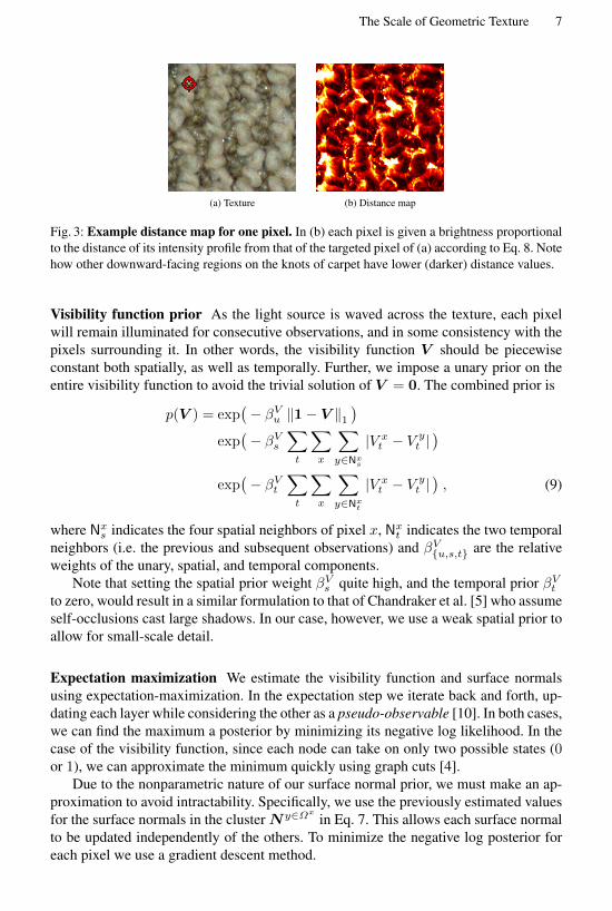
Fig. 3 shows the distance map for one pixel that is located on the downward-facingslope of a carpet knot. As can be seen by the dark regions, this pixel has a low distancevalue to similarly oriented surface patches. The bright regions, on the other hand, cor-respond to areas that are not frequently illuminated at the same time, or seldom havesimilar intensity values.


(a) Texture (b) Distance map

Fig. 3: Example distance map for one pixel. In (b) each pixel is given a brightness proportionalto the distance of its intensity profile from that of the targeted pixel of (a) according to Eq. 8. Notehow other downward-facing regions on the knots of carpet have lower (darker) distance values.

Visibility function prior As the light source is waved across the texture, each pixelwill remain illuminated for consecutive observations, and in some consistency with thepixels surrounding it. In other words, the visibility function V should be piecewiseconstant both spatially, as well as temporally. Further, we impose a unary prior on theentire visibility function to avoid the trivial solution of V = 0. The combined prior is

p(V ) = exp(− βVu ‖1− V ‖1

)exp(− βVs

∑t

∑x

∑y∈Nx

s

|V xt − Vyt |)

exp(− βVt

∑t

∑x

∑y∈Nx

t

|V xt − Vyt |), (9)

where Nxs indicates the four spatial neighbors of pixel x, Nxt indicates the two temporalneighbors (i.e. the previous and subsequent observations) and βVu,s,t are the relativeweights of the unary, spatial, and temporal components.

Note that setting the spatial prior weight βVs quite high, and the temporal prior βVtto zero, would result in a similar formulation to that of Chandraker et al. [5] who assumeself-occlusions cast large shadows. In our case, however, we use a weak spatial prior toallow for small-scale detail.

Expectation maximization We estimate the visibility function and surface normalsusing expectation-maximization. In the expectation step we iterate back and forth, up-dating each layer while considering the other as a pseudo-observable [10]. In both cases,we can find the maximum a posterior by minimizing its negative log likelihood. In thecase of the visibility function, since each node can take on only two possible states (0or 1), we can approximate the minimum quickly using graph cuts [4].

Due to the nonparametric nature of our surface normal prior, we must make an ap-proximation to avoid intractability. Specifically, we use the previously estimated valuesfor the surface normals in the cluster Ny∈Ωx

in Eq. 7. This allows each surface normalto be updated independently of the others. To minimize the negative log posterior foreach pixel we use a gradient descent method.


Carpet Carpet detail Toast Toast detail

Trad

ition

alO

urm

etho

d

Fig. 4: Resulting normal field comparison. Note the increased detail of our method.

In the maximization step, we update the noise variance σ2 using the maximum like-lihood estimator. These two steps, updating the latent values, and maximizing the like-lihood, are iterated until convergence which we define as an average change in surfaceorientation of less than 1.

In Fig. 2 we show the result of our method on a synthetic scene of several spheresembedded in a plane. In addition to self-occlusion, as the light passes over the scene,each sphere casts large shadows on the background plane. These shadows result inerroneous normal estimations around each sphere when the traditional approach is used.On the right hand side of the figure we show a series of normal vectors from one sliceof the resulting normal fields. Note how our method is able to accurately recover thesharp change from the background plane to the sphere. In Fig. 4 we compare our resultfor two real-world textures to the result using the traditional method. Qualitatively, onecan see the increased clarity that results from our method over the traditional approach.

4 Encoding geometric texture

With the exception of sharp depth discontinuities, the geometry of texture is well de-scribed by the normal field. This normal field, however, will change dramatically as thetexture is rotated, or moved towards or away from the viewer. An ideal representationof texture geometry will be both rotation-invariant and will encode its scale variability.

4.1 Rotation-invariant base representation

In order to obtain a rotation-invariant representation of texture geometry, we first adjustthe normal field so that the global surface normal (i.e., the mean normal) is alignedwith the positive z-axis. This accounts for small out-of-plane rotations of the texture.As shown in Fig. 5c, we then form a normalized two-dimensional histogram h(φ, θ)from the azimuth angle φ and polar angle θ of each surface normal. For our experi-ments, we quantize the polar and azimuth angles into 100 bins. In Fig. 5c we showone such histogram in which brighter regions correspond to higher values. We can seethat the texture is relatively coarse by observing that it has a highly structured groupingof normals. In this histogram, a rotation about the mean normal corresponds to a shift


(a) Carpet texture (b) Normal field (c) Histogram (d) FFT amp.

Fig. 5: Steps to form base representation. After computing the surface normals (b), we build a2D histogram (c) from the polar and azimuth angles of each normal vector. We use the rotation-invariant amplitude of the frequency domain (d) as our base representation.

(a) Near (b) Far (c) Estimated

Fig. 6: Comparison of real and estimated scale. When a texture (in this case, a cloth) is imagedat an increased distance, the apparent normal field becomes more coherent (b). We approximatethis by smoothing the original normal field (a). The resulting histogram (c) is quite similar to thehistogram of the observed texture.

along the horizontal (azimuth) axis. The final step in our base representation is to applyFourier transform to the histogram. The amplitude of the transform, shown in log-spacein Fig. 5d, is then a rotation invariant characterization of the normal field.

We define the similarity of two such frequency representations using the Jensen-Shannon divergence [14]. Given two surface textures A and B, we first compute theirrespective rotation-invariant representations HA(u, v) and HB(u, v). We then definetheir similarity as the Jensen-Shannon divergence of HA and HB

J (HA, HB) =1

2

(K(HA, C) +K(HB , C)

), (10)

where HA and HB are the normalized distributions

HA =HA∑∑|HA|

HB =HB∑∑|HB |

, (11)

C is their mean, and K is the Kullback-Leibler divergence.

4.2 Scale-space representation

In Fig. 6 we show the surface normal field for a cloth at two distances. On the far left, thecloth is relatively close to the camera, and in the middle the cloth has been moved twicethe distance away. Although the geometry of the cloth has not changed, the number of


Incr

emen

tals

moo

thin

g

Scal

e

Base normals

Base normalsBase representation

Base representation

(a) Normal fields (b) Our representation

Fig. 7: Building of scale-space representation. We represent the scale space of geometric texturewith frequency histograms (b) built from the polar histogram (not shown) of the incrementallysmoothed normal field (a).

microfacet surface normals subtended by each pixel has increased. In other words, asscale increases, the appearance of each pixel is determined by an increasing number ofsurface orientations. In effect, the average surface normal captured by a given pixel iscomputed across a greater area as scale increases. This observation, also underlying therecent work on geometric scale space of range images [1, 18], motivates our approachto modeling the scale variability of geometric texture.

We describe the scale space of geometric texture by filtering the surface normalfield with Gaussian kernels of increasing standard deviation. In Fig. 6 we illustrate theresult of this approach by comparing the resulting normal histogram (c) with that of thetexture at a greater distance (b). The result is quite similar to the observed histogram.

Fig. 7 summarizes the creation process of our scale-space representation. Starting inthe lower left, we begin with the observed normal field of texture. As shown in (a), wethen smooth this normal field at small intervals. At each interval, the polar histogramis formed and its Fourier transform is computed (b). This process is repeated until thenormal field is sufficiently coherent (has an angular standard deviation of 2). Note thatas this happens, the polar histogram becomes nondescript, and corresponding frequencyimage flattens out, as can be seen at the top of the stack. Smooth textures, whose normalfields are already quite coherent, require few scales to describe their scale variability,while coarse textures will have larger stacks.

5 Classification

We evaluate the effectiveness of our rotation-invariant scale-space representation oftexture geometry by performing classification on a new database.

5.1 Classifying a query texture

When a query texture is imaged, and its normal field is estimated, classification isperformed on its frequency amplitude histogram. In order to find the correct texture,we must also find the correct scale. One approach would be to compute the similarity(Eq. 10) between the query texture and every scale of every database texture. Needless


(a) Base distance, no rotation (b) Assorted distances and rotations

Fig. 8: Select database samples. Each of our 20 textures is imaged with 30 combinations oforientation and distance.

to say, this process quickly becomes too computationally expensive as the number oftextures and scales increases. To more quickly estimate the likely textures we first com-pare the total energy of the query texture to that of each database texture at each scale.The total energy is computed as the sum of the unnormalized frequency amplitudes.

5.2 Geometric texture database

As depicted in Fig. 8, we introduce a new database that covers 20 textures at differentdistances, with different in-plane and out-of-plane rotations1. To our knowledge, thisis the only public database that offers multiple distances for each texture in addition tomultiple in-plane and out-of-plane rotations. Our database, which contains stochasticas well as regular textures, includes organic materials such as bark and toast, wovenmaterials such as cloth crocheted fabric, and synthetic materials such as a carpet andsandpaper. For practical reasons, we did not construct a lighting apparatus for eachdistance. Instead, each dataset was lit by manually waving a light source around in aspiral pattern like the one shown in Fig. 1b. The lighting direction was estimated usinga reflective sphere. Each dataset consists of approximately 65 images. Every effort wasmade to keep the distance from the subject constant, but some amount of light attenua-tion will necessarily be present. To address this, each image is white-balanced using thelight source direction and a white paper in the scene. Since each texture is imaged withmore than 2, 000 different combinations of orientation, distance, and lighting direction,it is also useful for appearance modeling.

6 Experimental validationDistance For each texture in the model database, acquired at a distance D1, we acquiredadditional real data to be used as query instances for classification at two increasingdistances D2 and D3. All 20 query textures at D2 were classified correctly, while 19were correctly classified at D3. These are the the starting points in the top left of Fig. 9.

Noise Fig. 9 shows the robustness of our method to increasing levels of Gaussian noisein the normal field. The horizontal axis corresponds to the standard deviation of the

1 This database is available on-line at http://cs.drexel.edu/˜kon/texture.


0%

10%

20%

30%

40%

50%

60%

70%

80%

90%

100%

0% 1% 2% 3% 4% 5% 6% 7% 8% 9% 10% 11% 12% 13% 14% 15%

Distance1Distance2Distance3

Fig. 9: Recognition rates under increasing Gaussian noise. The horizontal axis is the standarddeviation of Gaussian noise added to the normal field. A sample region is shown for every thirdlevel of noise to illustrate the degree of corruption. Note that high accuracy is achieved even withsignificant corruption.

0%

10%

20%

30%

40%

50%

60%

70%

80%

90%

100%

15 30 45 60 75 90

Distance1Distance2

(a) In-plane rotation

0%

10%

20%

30%

40%

50%

60%

70%

80%

90%

100%

10 20 30 40 50 60

Distance1Distance2

(b) Out-of-plane rotation.

Fig. 10: Recognition rates for rotations Out-of-plane rotations expose previously unseen struc-tures, causing novel normal fields which are more challenging to classify. Although recognitionrates decline slightly at increased angles, high accuracy is persistent.

Gaussian noise applied to each dimension of normal field. Below the graph are samplepatches of a normal field at every third level of noise corruption. The fourth samplepatch shows the high degree of noise at σ = 9%. As shown in red, at this level 70% ofthe original textures are classified correctly. The blue and green lines correspond to theincreased distances of D2 and D3, respectively. Since each surface normal captures anincreased amount of surface area at these distances, noise has a greater effect.

In-Plane Rotation At distances D1 and D2 we rotated each texture 6 times in incre-ments of 15, stopping at a rotation of 90. Moving beyond 90 would be redundant,since the same result can be achieved by rotating the images 90. Overall, at distance D1we correctly classify 88% of the 120 query textures, and at distance D2 we correctlyclassify 81% of the query textures. In Fig. 10a we show the results for each rotationincrement.

Out-of-Plane Rotation At distances D1 and D2 we performed out-of-plane rotationsas well. These were done in increments of 10, stopping at 60. The results are summa-rized in Fig. 10b. Out-of-plane rotations present a unique challenge in that the rotationsexpose geometry that was previously hidden. In essence, out-of-plane rotations presentnovel textures as the side of the original texture becomes visible.


15 30 45 60 75 90∑

10 3/3 5/5 3/5 3/4 1/1 1/2 16/20

20 4/5 2/2 1/2 1/2 2/6 1/3 11/20

30 0/4 3/4 1/2 1/2 2/4 4/4 11/20∑7/12 10/11 5/9 5/8 5/11 6/9 38/60

Out

-of-

plan

ero

tatio

nan

gle

In-plane rotation angle

Table 1: Recognition rates for combinations of in-plane and out-of-plane rotations. For quickinspection, higher recognition rates are given a brighter background coloring. The last row andcolumn are sums. Note the high success rates for the top row and upper left region.

Arbitrary Rotations At distance D3 we tested 3 arbitrary combinations of in-planeand out-of-plane rotations for each texture. Table 1 shows the results of all 60 tests.Each row corresponds to an increased out-of-plane rotation angle, while each columncorresponds to an increased in-plane rotation angle. Each entry in the table shows thetotal correct classifications and the number of experiments run with that combinationof in-plane and out-of-plane rotation angles as a fraction. The shading of each cellindicates the overall success rate. Note that successful cases tend to have lower out-of-plane rotations, as expected.

7 Conclusion

In this work we have directly studied the geometry of texture. Through careful analysisof its two key characteristics—self similarity and scale variability—we have derived aphotometric stereo method specifically tailored to exploit the repetitive nature of texturegeometry, and have introduced a compact representation for the scale space of geomet-ric texture. To evaluate our methods we have also introduced an extensive new texturedatabase. Experimentally, we have shown that our compact scale-space representationis highly discriminative. We believe these results provide a sound foundation to explorethe use of geometric texture in longstanding problems in computer vision, includingexploiting texture geometry to aid object recognition and scene understanding.

Acknowledgments This work was supported in part by the Office of Naval Research grantN00014-11-1-0099, and the National Science Foundation awards IIS-0746717 and IIS-0964420.

References

1. P. Bariya, J. Novatnack, G. Schwartz, and K. Nishino. 3D Geometric Scale Variability inRange Images: Features and Descriptors. Int’l Journal of Computer Vision, 99:232–255,September 2012.

2. S. Barsky and M. Petrou. Classification of 3D Rough Surfaces Using Color and GradientInformation Recovered by Color Photometric Stereo. In SPIE Conf. on Visualization andOptimization Techniques, 2001.


3. S. Barsky and M. Petrou. The 4-Source Photometric Stereo Technique For Three-Dimensional Surfaces in the Presence of Highlights and Shadows. IEEE Trans. on PatternAnalysis and Machine Intelligence, 25(10):1239–1252, Oct. 2003.

4. Y. Boykov and V. Kolmogorov. An Experimental Comparison of Min-Cut/Max-Flow Algo-rithms for Energy Minimization in Vision. IEEE Trans. on Pattern Analysis and MachineIntelligence, 26(9):1124–1137, Sept. 2004.

5. M. Chandraker and S. Agarwal. ShadowCuts: Photometric Stereo with Shadows. In IEEEInt’l Conf. on Computer Vision and Pattern Recognition, pages 1–8, 2007.

6. M. Chantler, M. Schmidt, M. Petrou, and G. McGunnigle. The Effect of Illuminant Rotationon Texture Filters: Lissajous’s Ellipses. In European Conf. on Computer Vision, pages 289–303, 2002.

7. F. Cohen, Z. Fan, and M. Patel. Classification of Rotated and Scaled Textured Images UsingGaussian Markov Random Field Models. IEEE Trans. on Pattern Analysis and MachineIntelligence, 13(2):192–202, Feb. 1991.

8. K. J. Dana and S. K. Nayar. 3D Textured Surface Modeling. In IEEE Workshop on the Inte-gration of Appearance and Geometric Methods in Object Recognition, pages 44–56, 1999.

9. S. R. Fountain, T. N. Tan, and K. D. Baker. A Comparative Study of Rotation InvariantClassification and Retrieval of Texture Images. In British Machine Vision Conference, pages266–275, 1998.

10. J. Kim and R. Zabih. Factorial Markov Random Fields. In European Conf. on ComputerVision, pages 321–334, 2002.

11. S. Koppal and S. Narasimhan. Clustering appearance for scene analysis. In IEEE Int’l Conf.on Computer Vision and Pattern Recognition, volume 2, pages 1323–1330, 2006.

12. S. Lazebnik, C. Schmid, and J. Ponce. Affine-Invariant Local Descriptors and NeighborhoodStatistics for Texture Recognition. In IEEE Int’l Conf. on Computer Vision, 2003.

13. T. Leung and J. Malik. Recognizing Surfaces Using Three-Dimensional Textons. In IEEEInt’l Conf. on Computer Vision, pages 1010–1017, 1999.

14. J. Lin. Divergence Measures Based on the Shannon Entropy. IEEE Trans. on InformationTheory, 37(1):145–151, 1991.

15. G. McGunnigle and M. Chantler. Rough Surface Classification Using Point Statistics fromPhotometric Stereo. Pattern Recognition Letters, 21:593–604, June 2000.

16. S. Nayar, K. Ikeuchi, and T. Kanade. Shape from Interreflections. Int’l Journal of ComputerVision, 6(3):173–195, Aug. 1991.

17. S. Nayar, G. Krishnan, M. D. Grossberg, and R. Raskar. Fast Separation of Direct andGlobal Components of a Scene using High Frequency Illumination. ACM Trans. on Graph-ics, 25(3):935–944, July 2006.

18. J. Novatnack and K. Nishino. Scale-Dependent 3D Geometric Features. In IEEE Int’l Conf.on Computer Vision, pages 1–8, 2007.

19. A. Penirschke, M. Chantler, and M. Petrou. Illuminant Rotation Invariant Classification of3D Surface Textures Using Lissajous’s Ellipses. In Intl. Workshop on Texture Analysis andSynthesis, 2002.

20. M. Smith. The analysis of surface texture using photometric stereo acquisition and gradientspace domain mapping. Image and vision computing, 17(14):1009–1019, 1999.

21. K. Sunkavalli, T. Zickler, and H. Pfister. Visibility Subspaces: Uncalibrated PhotometricStereo with Shadows. In European Conf. on Computer Vision, pages 251–264, 2010.

22. M. Varma and A. Zisserman. Classifying Images of Materials: Achieving Viewpoint andIllumination Independence. In European Conf. on Computer Vision, pages 255–271, 2002.

23. R. J. Woodham. Photometric Method for Determining Surface Orientation from MultipleImages. Optical Engineering, 19(1):139–144, 1980.

24. T.-P. Wu and C.-K. Tang. Photometric Stereo Via Expectation Maximization. IEEE Trans.on Pattern Analysis and Machine Intelligence, 32(3):546–560, Mar. 2010.

the scale of geometric texture - drexel ccikon/publication/goxholm_eccv12_geomtext...the scale of...

Documents