The Sarnak Conjecture: Orthogonality of the Mobius Function on

Bounded Depth Circuits

Octav DragoiThesis Advisor - Arul Shankar

March 30, 2016

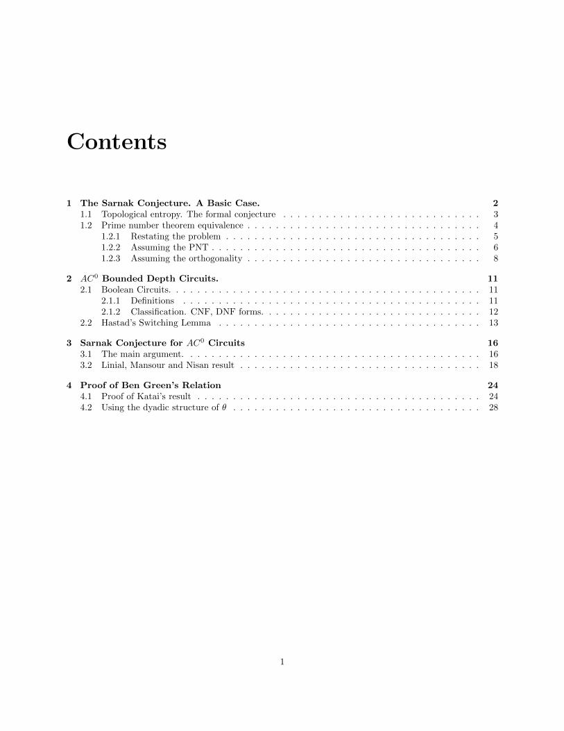
Contents

1 The Sarnak Conjecture. A Basic Case. 21.1 Topological entropy. The formal conjecture . . . . . . . . . . . . . . . . . . . . . . . . . . . . 31.2 Prime number theorem equivalence . . . . . . . . . . . . . . . . . . . . . . . . . . . . . . . . . 4

1.2.1 Restating the problem . . . . . . . . . . . . . . . . . . . . . . . . . . . . . . . . . . . . 51.2.2 Assuming the PNT . . . . . . . . . . . . . . . . . . . . . . . . . . . . . . . . . . . . . . 61.2.3 Assuming the orthogonality . . . . . . . . . . . . . . . . . . . . . . . . . . . . . . . . . 8

2 AC0 Bounded Depth Circuits. 112.1 Boolean Circuits. . . . . . . . . . . . . . . . . . . . . . . . . . . . . . . . . . . . . . . . . . . . 11

2.1.1 Definitions . . . . . . . . . . . . . . . . . . . . . . . . . . . . . . . . . . . . . . . . . . 112.1.2 Classification. CNF, DNF forms. . . . . . . . . . . . . . . . . . . . . . . . . . . . . . . 12

2.2 Hastad’s Switching Lemma . . . . . . . . . . . . . . . . . . . . . . . . . . . . . . . . . . . . . 13

3 Sarnak Conjecture for AC0 Circuits 163.1 The main argument. . . . . . . . . . . . . . . . . . . . . . . . . . . . . . . . . . . . . . . . . . 163.2 Linial, Mansour and Nisan result . . . . . . . . . . . . . . . . . . . . . . . . . . . . . . . . . . 18

4 Proof of Ben Green’s Relation 244.1 Proof of Katai’s result . . . . . . . . . . . . . . . . . . . . . . . . . . . . . . . . . . . . . . . . 244.2 Using the dyadic structure of θ . . . . . . . . . . . . . . . . . . . . . . . . . . . . . . . . . . . 28

1

Chapter 1

The Sarnak Conjecture. A BasicCase.

The Mobius function is defined, as usual:

µ(n) =

1 n = 1(−1)k n = p1p2 . . . pk0 otherwise

The analytic behavior of this function is very important, with regard to prime numbers. The specificquestion of “orthogonality” with an integer sequence F (n), n ≥ 1 is important, since many questions inanalytic number theory are equivalent to particular cases of such orthogonality.

More specifically, we define the “orthogonality” of µ and F as the analytic behavior:∑n≤x

µ(n)F (n) = o(x) as x→∞

A function F which is orthogonal on µ is called deterministic, and nondeterministic otherwise.The main conjecture regarding the question of orthogonality is stated by Sarnak, that this is true for

functions that are well-behaved, in some sense which shall be defined in the next section. It has been provenfor some specific classes of functions, while the question is still open for some other classes.

A comprehensive list of classes for which the conjecture has been proven (in some cases very recently)can be found in [2].

• If F (n) ≡ 1, then the relation becomes: ∑n≤x

µ(n) = o(x)

which is equivalent to the prime number theorem. We shall prove this equivalence in the last sectionof this chapter.

• If F (n) is a periodic function, then the relation is equivalent to the prime number theorem in arithmeticsequences, or Dirichlet’s theorem.

• For F (n) a function computable by bounded depth circuits AC0 (to be defined later on), the fact thatSarnak’s conjecture holds is a recent result by Ben Green and the main focus of the thesis.

• F (n) = µ(n) is nondeterministic; namely, we have:

1

N

∑n≤N

µ2(n)→ 6

π2(1.1)

2

The proof for 1.1 can be found in [10], the following is an abridged version of it. The main idea is thatthe asymptotic limit 1

N

∑x≤N µ

2(x) represents the probability that a number is squarefree, that is, it does

not belong to any arithmetic progression of ratio p2. Formally, let χp2 be the characteristic function for thisprogression. Then, use the cutoff of the Taylor expansion series:

µ2(n) =∏p

(1− χp2(n))

= 1−∑p1

χp21(n) +

∑p1<p2

χp21(n)χp2

2(n)− · · ·+ (−1)k

∑p1<p2<···<pk

χp21(n)χp2

2(n) . . . χp2

k(n) + εk(n)

where εk(n) is the remainder term, for which limk→∞ εk(n) = 0. Average this equality for all n:

1

N

∑n≤N

µ(n) = 1−∑p1

1

p21

+∑p1<p2

1

(p1p2)2− · · ·+ (−1)k

∑p1<p2<···<pk

1

(p1p2 . . . pk)2+

∑n≤N

εk(n)

N

therefore, by passing to the limit in both N and k:

limn→∞

1

N

∑x≤N

µ2(x) =∏p

(1− 1

p2

)The product can be evaluated as well, by inverting it and breaking down the geometric series.∏

p

1

1− 1p2

=∏p

(1 +

1

p2+

1

p4+ . . .

)=∑n≥1

1

n2

=1

ζ(2)=π2

6

automatically implying 1.1.

1.1 Topological entropy. The formal conjecture

This section formalizes the definition of the Sarnak conjecture.

Conjecture 1.1 (Sarnak) The relationship:∑n≤x

µ(n)F (n) = o(x) as x→∞

holds for functions F that have zero topological entropy.

We now define the concept of topological entropy.For a function f : R→ C and for a given m ∈ N, look at the set:

Sm = {(f(n+ 1), f(n+ 1), . . . f(n+m))|n ∈ N} ⊂ Cm

and, for any ε > 0, define B(m, ε) to be the number of balls of radius ε under the standard metric of Cnecessary to cover Sm. Then the topological entropy σ of f is defined as:

σ = lim supm→∞

1

mlog (B(m, ε))

3

In other words, σ ≥ 0 is the least parameter such that, for any ε > 0 and for m→∞, Sm can be coveredby O(exp(σm + o(m))) balls of radius ε. Intuitively, if f is Boolean, the number of m-tuples considered incounting the size of Sm is 2m = exp(m log 2); the topological entropy σ represents the lowest factor that canreplace the log 2, as m goes to infinity.

A few examples:

• The constant function f ≡ 1 clearly has |Sm| = 1, and therefore has zero entropy. This case will bediscussed in detail below.

• For a periodic function of period P , the set Sm can have at most P different elements. In terms of theSarnak conjecture, this case corresponds to the PNT applied in arithmetic progressions.

• Predictably, µ does not have zero entropy; it can be calculated that its entropy is actually 6π2 log 2.

This is to be expected, agreeing with 1.1, yet the proof is highly nontrivial. It can be found in [11].

1.2 Prime number theorem equivalence

This section will prove that the Mobius orthogonality relation:∑n≤x

µ(n) = o(x)

is equivalent to the prime number theorem, stated as:∑p≤x

1 = (1 + o(1))x

log(x)

The following proof loosely follows the sketch set forth by Terence Tao in [2], filling in the gaps andunproven claims.

We introduce the von Mangoldt function Λ(n), defined as:

Λ(n) =

{log p n = pk

0 otherwise

Define the following sums that will be of interest for us.

π(x) =∑p≤x

1

ν(x) =∑p≤x

log(p)

Ψ(x) =∑n≤x

Λ(n)

For example, it is relatively straightforward to obtain a weaker bound on π(x). Notice that the binomial(2nn

)is smaller than 4n and also that it is a multiple of all primes between n and 2n. Therefore:

n log 4 ≥∑

n≤p≤2n

log p ≥∑

n≤p≤2n

log n

n log 4

log n≥

∑n≤p≤2n

1

4

and, ultimately, by summing this up repeatedly:

log 4

log2 n−1∑k=0

( n2k

log n2k

)≥ π(n)

We want to prove the sum on the left is actually O( nlogn ). To do this, split it in half, and analyze each

section separately:

1

log 4π(n) ≤

log2 n−1∑k=0

( n2k

log n2k

)=

log2 n2∑

k=0

( n2k

log n− k log 2

)+

log2 n−1∑k=

log2 n2

( n2k

log n− k log 2

)

≤

log2 n2∑

k=0

(n2k

log n− logn2

)+

log2 n−1∑k=

log2 n2

(n√n

1

)

≤ n

log n

log2 n2∑

k=0

1

2k+

log2 n−1∑k=

log2 n2

√n

≤ O(

n

log n

)+O

(√n log n

)

In conclusion:

π(n) = O

(n

log n

)(1.2)

which is a weaker version of the prime number theorem:

π(n) =n

log n+ o

(n

log n

)

1.2.1 Restating the problem

We shall prove that π and Ψ are essentially proportional to each other, thus allowing us to restate the primenumber theorem, namely that:

π(x) = (1 + o(1))x

log(x)⇐⇒ Ψ(x) = (1 + o(1))x

For one side of the asymptotic inequality, break down Ψ as follows:

Ψ(x) =∑n≤x

Λ(n) =∑

p≤x, pα<x<pα+1

α log(p) =∑p≤x

log pα ≤ log(x)π(x)

5

For the other side, write as follows:

Ψ(x) ≥ ν(x) =

log2 x∑k=0

∑x

2k+1≤p≤x

2k

log p

≥log2 x∑k=0

∑x

2k+1≤p≤x

2k

log(x)− (k + 1) log 2

≥ π(x) log(x)− log 2

log2 x∑k=0

(k + 1)∑

x

2k+1≤p≤x

2k

1

≥ π(x) log(x)− log 2

log2 x∑k=0

(k + 1)(π( x

2k

)− π

( x

2k+1

))

≥ π(x) log(x)− log(2)

log2 x∑k=0

π( x

2k

)Pick 0 ≤ A ≤ log2 x, and split up the sum in two pieces: up to A, and beyond A. Then, by using the

simpler estimation (1.2) that we proved π(x) = O( xlog x ) we can deduce:

log2 x∑k=0

π( x

2k

)=

A∑k=0

π( x

2k

)+

log2 x∑k=A+1

π( x

2k

)≤ A ·O

(x

log x

)+ (log2 x−A)O

( x2A

log x−A log 2

)By picking a suitable A, we can ensure that this function is o(x). For example, pick A = log log x:

log2 x∑k=0

π( x

2k

)≤ log log x ·O

(x

log x

)+ (log2 x− log log x)O

( xlog x

log x− log log x log 2

)

≤ O(x log log x

log x

)+O

( xlog x log x

log x

)≤ o(x)

Therefore the other inequality is proven, and we can conclude:

π(x) log(x) ≥ Ψ(x) ≥ π(x) log(x)− o(x)

and the equivalence is now straightforward, via (1.2):

π(x) = (1 + o(1))x

log(x)⇐⇒ Ψ(x) = (1 + o(1))x

1.2.2 Assuming the PNT

Start with the identity:

−µ(n) log(n) =∑d|n

µ(d)Λ(n

d) (1.3)

6

This identity comes from a double application of the Mobius inversion formula. The formula itself statesthat, for f, g two arithmetic functions, we have the following property:

f(n) =∑d|n

g(d) ⇐⇒ g(n) =∑d|n

µ(d)f(n/d), ∀n ∈ N

A proof, and further detaliation of this basic theorem in number theory can be found in many sources,such as [12]. For this specific application, the process follows:

log(n) =∑d|n

Λ(d) =⇒ Λ(n) =∑d|n

µ(d) log(n

d)

=⇒ Λ(n) = log n∑d|n

µ(d) +∑d|n

−µ(d) log d

=⇒ Λ(n) =∑d|n

−µ(d) log d

=⇒ −µ(n) log(n) =∑d|n

µ(d)Λ(n

d)

Sum (1.3) for 1 ≤ n ≤ x:

−∑n≤x

µ(n) log(n) =∑d≤x

µ(d)∑

m≤x/d

Λ(m) =∑d≤x

µ(d)Ψ(x

d)

Let us evaluate the behavior of the right term. Assuming that we know the prime number theorem, thatis, for any ε and sufficiently large x/d:

Ψ(x

d) = (1 + o(1))

x

d= (1 +O(ε))

x

d

the right term evaluates to:∣∣∣∣∣∣∑d≤x

µ(d)x

d+ µ(d)o(1)

x

d

∣∣∣∣∣∣ ≤ x∣∣∣∣∣∣∑d≤x

µ(d)

d

∣∣∣∣∣∣+ x · o(1)∑d≤x

1

d

The unknown sum can be evaluated by summing the identity 1n=1 =∑d|n µ(d) for n ≤ x and observing:

1 =∑d≤x

µ(d)⌊xd

⌋=∑d≤x

µ(d)x

d−∑d≤x

µ(d){xd

}(1.4)

1 ≥ x

∣∣∣∣∣∣∑d≤x

µ(d)

d

∣∣∣∣∣∣− x+ 1

Therefore the right term evaluates to:∣∣∣∣∣∣−∑n≤x

µ(n) log(n)

∣∣∣∣∣∣ ≤ x∣∣∣∣∣∣∑d≤x

µ(d)

d

∣∣∣∣∣∣+ x · o(1)∑d≤x

1

d≤ x+ o(x log(x)) = o(x log(x))

7

Obtain the final desired relation through summation by parts:

o(x log(x)) =

∣∣∣∣∣∣∑n≤x

µ(n) log(n)

∣∣∣∣∣∣ =

∣∣∣∣∣∣log(x)

∑n≤x

µ(n)

−∑n≤x

∑d≤n

µ(d)

logn+ 1

n

∣∣∣∣∣∣≥ log(x)

∣∣∣∣∣∣∑n≤x

µ(n)

∣∣∣∣∣∣−∑n≤d

∣∣∣∣∣∣∑d≤n

µ(d)

∣∣∣∣∣∣(n+ 1

n− 1

)

≥ log(x)

∣∣∣∣∣∣∑n≤x

µ(n)

∣∣∣∣∣∣−∑n≤x

n · 1

n

o(x) ≥

∣∣∣∣∣∣∑n≤x

µ(n)

∣∣∣∣∣∣1.2.3 Assuming the orthogonality

We will now prove the other implication:∑n≤x

µ(n) = o(x) =⇒ Ψ(x) = (1 + o(1))x

Introduce the following identities, that come directly from the Mobius inversion formula:

log(n) =∑d|n

Λ(d) =⇒ Λ(n) =∑d|n

µ(d) log(n

d)

τ(n) =∑d|n

1 =⇒ 1 =∑d|n

µ(d)τ(n

d)

Expand Ψ− x =∑n≤x(Λ(n)− 1) using these identities:∑n≤x

Λ(n)− 1 =∑n≤x

∑d|n

µ(d)(logn

d− τ(

n

d))

=∑

m,n:mn≤x

µ(n)(τ(m)− log(m))

=∑n≤x

µ(n)

∑m≤x/n

τ(m)−∑

m≤x/n

log(m)

Estimate the two sums. The latter sum is relatively straightforward, through Stirling’s formula:∑

m≤x/d

log(m) = log(xd

)! =

x

dlog(xd

)− x

d+O

(log(xd

))(1.5)

The former can be estimated through Dirichlet’s hyperbola method. This is described in many classical

8

number theory books, for example in [6], page 22. Use x = x/d for easier notation:∑m≤x

τ(m) =∑m≤x

∑ab=m

1 · 1 =∑a≤√x

∑b≤x/a

1 +∑b≤√x

∑a≤x/b

1−∑a≤√x

∑b≤√x

1

=∑a≤√x

(xa

+O(1))

+∑b≤√x

(xb

+O(1))−

∑a≤√x

1

2

= 2x∑n≤√x

1

n+O(

√x)− (

√x+O(1))2

= 2x

(log(√x) + γ +O

(1√x

))− x+O(

√x)

= x log x+ (2γ − 1)x+O(√x)

and so: ∑m≤x

τ(m) = x log x+ (2γ − 1)x+O(√x) (1.6)

Therefore, from (1.5) and (1.6) we can use the following in estimating Ψ− x:

∑m≤x/n

τ(m)−∑

m≤x/n

log(m) = 2γx

m+O

(√x

m

)

Ψ(x)− x =∑n≤x

Λ(n)− 1 =∑n≤x

µ(n)

(2γx

n+O

(√x

n

))

= 2γx∑n≤x

µ(n)

n+∑n≤x

O

(√x

n

)µ(n)

Estimate the two sums, in order to conclude that Ψ(x)− x = o(x). For the first one, use relation (1.4):

1 = x∑d≤x

µ(d)

d−∑d≤x

µ(d){xd

}Prove that

∑d≤x µ(d)

{xd

}= o(x). Let A > 0, and cut the sum off before applying summation by parts.

Use the estimation∑d≤x µ(d) = o(x):

∑x/A≤d≤x

µ(d){xd

}=∑d≤x

µ(d) +∑n≤x

∑d≤n

µ(d)

({ x

n+ 1

}−{xn

})

= o(x) +∑

1≤i≤A

∑x/(i+1)≤n<x/i

∑d≤n

µ(d)

({ x

n+ 1

}−{xn

})= o(x) +

∑1≤i≤A

(o(xi

)·O(1)

)= o(x)

so, therefore:

x∑d≤x

µ(d)

d= 1 +

∑d≤x

µ(d){xd

}=⇒

∑d≤x

µ(d)

d= o(1)

9

For the second sum, use the standard integral approximation that shows∑n≤x

1n1/2 = O(x1/2), adapted

to show that∑n≤xO

(1

n1/2

)= O(x1/2):

∑n≤x

O

(√x

n

)µ(n) =

√x∑n≤x

O

(1√n

)= O(x)

To put everything together, it is required to split the sum in two parts. For simplicity, denote F(xn

)=∑

m≤x/n τ(m)− log(m) and split the sum according to a variable parameter 1 ≤ A ≤ x:

∑n≤x

Λ(n)− 1 =∑n≤x

µ(n)

∑m≤x/n

τ(m)−∑

m≤x/n

log(m)

=

∑n≤x/A

µ(n)F(xn

)+

x∑n≥x/A

µ(n)F(xn

)

=

2γx

A

∑n≤x/A

µ(n)

n+∑

n≤x/A

O

(√x

n

)µ(n)

+

A∑k=1

F (k)

xk∑

n= xk+1

µ(n)

= O( xA

)+

A∑k=1

F (k)o(x) = O( xA

)+Ao(x)

Since this is true for any A, we can let x→∞ and A→∞ such that Ao(x) = o(x) and O(x/A) = o(x)at the same time.

10

Chapter 2

AC0 Bounded Depth Circuits.

The purpose of this chapter is to set up the theoretical background for basic circuit complexity theory, andto understand what is a bounded depth circuit. In [3], Ben Green proves that the Sarnak conjecture holdsfor functions F : N → {−1, 1} such that F (x) is computed from the binary digits of x by a AC0 boundeddepth circuit. We shall define AC0 and similar other circuit classes, according to standard circuit complexitytheory.

This chapter aims to provide a background on circuits and circuit complexity theory, and to prove animportant lemma used to study them. In the next chapter, we will prove the Sarnak for AC0 circuits.

2.1 Boolean Circuits.

2.1.1 Definitions

Definition 2.1 A boolean circuit is a directed acyclic graph C = (V,E), where the nodes are partitioned in3 types: inputs, gates and outputs. Each node has a set of edges that are incoming, these form the fan-in ofthe node; similarly, the outgoing edges form the fan-out.

Denote the number of nodes |V | = n+ s+ r, such that there are n inputs, s gates and r outputs. Then theset of input nodes X = {x1, x2, . . . , xn} is regarded as a set of boolean input variables; each of these nodeshas a fan-in of size 0. The set of output nodes Y = {y1, y2, . . . , yr} is regarded as the output of the booleancircuit; each of the nodes has fan-in 1 and fan-out 0.

Now, we want this circuit to be able to compute a multi-variate boolean function F : Zn2 → Zr2. To do

this, equip each gate g ∈ V with a boolean function f : Zi(g)2 → Z2, where i(g), o(g) are the sizes of itsfan-in and fan-out, respectively. These functions take as inputs the values of the nodes from the fan-in of g,compute a result and distribute it further, to the fan-out of g. In practice, these functions are either one ofthe standard logical gates and, or, not.

This is a step-by-step computation, until all gates have an assigned value. Then, the value of each outputis equal to the value of the gate from its fan-in (there is only one).

Claim 2.2 The process does not get stuck.

Indeed, suppose it did, and there was a configuration in which there was no gate for which all inputs areknown. Pick a gate g0; a gate from its fan-in g1 has an unknown value. Do the same for g1, pick a g2 fromits fan-in that is not computed. Continue:

g0 ← g1 ← g2 ← . . .

Since the number of gates with unknown inputs is finite, this infinite chain will close at some point, thusyielding a cycle in a DAG, a contradiction.

11

�Define the size of a circuit as the number of gates it contains. Also define the depth of a circuit as the

longest path from an input to an output. These concepts will be useful in characterizing circuit families,which we will define now.

A boolean circuit has a set number of inputs, but suppose one wishes to compute a function over inputsof any cardinality:

F : Z =⋃n≥1

Zn2 → Z2

Definition 2.3 Define a family of circuits (Cn)n≥1 such that Cn has n inputs and computes F on thesubset Zn2 . One can analyze asymptotic behaviors of the sizes and widths of Cn as n goes to infinity, andcharacterize circuit families based on them.

Another important concept in classical circuit complexity theory is computability. Intuitively, we wantto restrict the families of circuits to only contain circuits that can be computed within a limited amount oftime, by a Turing machine, so that the circuits can actually be built fairly efficiently.

For example, a circuit family (Cn)n≥1 is logspace uniform if the following functions are all computablewithin O(log n) space. Note that the cumulative information of all these functions yield (Cn)n≥1 precisely:

• size(n), the function that returns m the size of Cn.

• type(n, k), 1 ≤ k ≤ m, the function that returns the type of the node i. In other words, it returnseither and, or, not, output(i), input(j), depending on whether node k is a gate, the ith output orthe jth input respectively.

• edge(n, i, j) that returns 1 if there is an edge from i to j and 0 otherwise.

Changing the required space to compute these functions yield different uniformity classes; for example,a P-uniform family can be computed by functions in O(nk) space for some k. But, for our purposes, we willuse logspace uniformity to define the circuit classes.

2.1.2 Classification. CNF, DNF forms.

Now we will define the main classification classes of boolean circuits, as defined in the previous section.Intuitively, we are interested to define families of circuits that have limited depth, polynomial size and arealso logspace uniform.

Definition 2.4 We define the class of NCi, i ∈ N as the class of families of circuits (Cn)n≥1 that respectsthe following conditions:

• each gate has at most two inputs, and computes a standard function among and, or, not;

• has depth O(logi n);

• has size O(nk) for some k ∈ N;

• is logspace-uniform as defined above.

The class is named after Nick Pippenger (Nick’s Class) by Steven Cook, in honor of the researcher ofcomplexity classes.

The ACi class is similarly defined after the NCi class, but where all gates are allowed to have an unlimitednumber of inputs, instead of simply two, therefore calculating and, or for a larger number of inputs.

In a circuit C belonging to a family from ACi, every gate is either a and or a or gate, with inputs thatare various such other gates. Of course, a and gate that has another and gate as an input can be mergedin the large one, and the same holds for or.

12

In studying this local structure, it makes sense to focus our attention on ands of or gates and vice-versa,on ors gates of and. Call the former type a CNF (conjunctive normal form) and the latter ones DNF(disjunctive normal forms).

Definition 2.5 Formally, a CNF on x1, x2, . . . xn is an and of ors such that:

f = T1 ∧ T2 ∧ · · · ∧ Tk,where xi1 ∨ · · · ∨ xin(i)

and a DNF is an or of ands, clearly, the symmetrical:

f = T1 ∨ T2 ∨ · · · ∨ Tk,where Ti = xi1 ∨ · · · ∨ xin(i)

Define the width of a CNF/DNF as the maximum size of its components Ti.Notice that, locally, a circuit in AC0 looks like a CNF or a DNF. The main idea behind this entire setup

is to show that there is significant cancellation within a circuit, and such an evaluation starts from analyzingthe behavior of the local CNF/DNF structure. For this purpose, the next section will introduce and proveHastad’s lemma, as defined by Hastad in [7] and proved in a simpler manner by Razborov in [8].

2.2 Hastad’s Switching Lemma

The lemma, presented by Johan Hastad in [7], switches a DNF into a CNF and vice-versa, in order to dothat in large circuits and collapse their depth at the expense of size. To do so, we connect both of theseconcepts with a third, common one. Define a decision tree in the ordinary way, where at each step the treebranches out with regards to a “decision”, that is, a boolean operation with one of the inputs. Naturally,one can associate a decision tree (DT) with a boolean function. Also, similarly to circuits, one can definethe depth of a DT as being the longest path from its root to one of its leaves.

Thus, CNFs and DNFs can be computed by decision trees. Denote DTdepth(f) as the depth of thesmallest circuit that computes the boolean function f .

Hastad’s lemma deals with the depth of DNFs under restrictions. A restriction ρ represents a mappingfrom the input variables x1, . . . , xn to the set {0, 1, ∗}. A restriction ρ applied to a function f yields afunction fρ on the variables that are sent to ∗, with the rest fixed to either 0 or 1.

A random restriction ρ with parameter 0 ≤ p ≤ 1 is a restriction where ρ(xi) is randomly set:

ρ(xi) =

∗ with probability p

0 with probability 1−p2

1 with probability 1−p2

Intuitively, we want to prove that a DNF suffers significant reductions under a restriction, in most cases.The formal statement of the lemma:

Theorem 2.6 Hastad’s switching lemma. Let f be a DNF of width w and n variables, and ρ a randomrestriction with parameter p = σn, σ ≤ 1/5. Then, for each parameter d:

Pr (DTdepth(fρ) > d) ≤ (10σw)d

We wish to show that there are relatively few bad restrictions ρ such that fρ requires a decision treewith depth greater than d to be computed. In other words, if B is the set of bad restrictions and Rp isthe set of all restrictions with cardinality p, then we wish to show that:

|B||Rp|

≤ (10σw)d

The cardinality of Rp is easily computable; it is(np

)2n−p. The main idea is to reduce the restriction

ρ ∈ Rp to another restriction ρ′ ∈ Rp−d, plus some “additional information” that would ensure injectivity.This set of “additional information” shall be defined later.

13

Definition 2.7 We shall now define, for a DNF f , its canonical decision tree. Such a tree will, in particular,have depth greater than DTdepth(f). If T1, T2, . . . , Tk are the terms of f , then take the first term T1, say ithas length d1, and order its literals. Construct a decision tree of depth d1 that passes through all the literalsof T1 in order. T1 is an and; therefore, exactly one of the end-paths corresponds to 1, where f is also 1. Forthe rest of the paths, continue calculating T2 similarly while omitting the already decided variables, and soon until the end.

A similar procedure is applied for fρ. Under ρ, many of the terms Ti will cancel out; it is enough for asingle literal in Ti to be set to 0, and the entire term is trivialized. Suppose that ρ does not kill the termsTi1 , . . . , Tik , and denote the non-trivial reductions under ρ of the terms Ti as Uj , 1 ≤ j ≤ k′. Therefore:

fρ = U1 ∨ U2 ∨ · · · ∨ Uk′

and one can build the canonical decision tree for this function. By hypothesis, the depth of this tree isgreater than d.

Definition 2.8 Now, define π as the lexicographical leftmost path of length greater than d, and consideronly its first d terms; that is, the first d variables that π restricts. Because the decision tree is still not trivial,this means that, under the restriction ρπ ∈ Rp−d which is the combined restriction of ρ and π, the functionfρπ is not decided. Unfortunately, using this new restriction will not be enough to recover ρ from ρπ, sinceit is difficult to see what belongs to this path and what not.

Instead, let us look at U1, U2, . . . Uk′ . Denote γi as the (unique) restriction that fixes Ui to 1, and πi thepart of π that fixes variables from γi. Assuming that π1 is not the entirety of π, note that βπ1 kills the termU1. Otherwise, since U1 is an and, all its literals fixed by π1 would also be fixed by γ1 in the same way, andat the end of π1 the term U1 would be undecided, which is impossible by definition; π1 ends and π2 beginswhen U1 is decided.

Continue this process and define γj , πj for each Tij , Uj . The restriction that we are looking for is:

ρ′ = ργ1γ2 . . . γk

Note that, because γj fixes the same number of variables as πj , ρ′ ∈ Rp−d, just as ρπ. Now we just have

to decide on the additional information that is to be added, so that ρ can be recovered from ρ′.

Claim 2.9 The function fρ′ fixes T1, T2, . . . Ti1−1 to 0, exactly as fρ does. Also, Ti1 is the first term thatfρ′ fixes to 1.

The first part of the claim is easy to establish, since ρ ⊂ ρ′ and Ti1 , by definition, is the first term not tobe fixed to 0. Also, by the definition of γ1, U1 is fixed to 1 and since Ti1 was undecided, now it is also fixedto 1.

After identifying i1, we want to identify which of the variables in Ti1 are fixed by γ1 and which do not.If |U1| = u1, then this information will require u1 logw bits of information, since |Ti1 | ≤ w and any positionfrom 1 to w can be encoded in logw bits of information. Also encode how π1 fixes these variables withu1 additional bits. Together with the encoding of u1 itself, needed to revert the operation, this amount ofinformation occupies a certain number of bits:

u1 logw + u1 + log u1 ≤ u1 logw + 2u1

Now, based on this information, we can retrieve γ1 from the knowledge of its variables and π1 as well,from the knowledge of its assignments. For the next step, consider ρ′1 = ρπ1γ2 . . . γk. Following the exactsame argument, the first term of f that this restriction fixes to 1 is Ti2 ., so the same procedure can beapplied. In u2 logw+ 2u2 bits, one can find out γ2, π2. Continue similarly until the end of the restriction π,when we determine the last γk. In total, all the γj should fix precisely d variables.

14

At this point, we have determined γ1, . . . , γk which means that we can recover ρ from ρ′. This constructionis in fact an injection:

Rp ↪→ Rp−d × Swhere S stands for the set of binary strings that encode the additional information needed to establish thereverse operation, as described. S has a total size of:

(u1 logw + 2u1) + (u2 logw + 2u2) + · · ·+ (uk logw + 2uk) = d logw + 2d

Claim 2.10 The size of the term on the right side is small enough so that the proportion of “bad” restrictionsis small as well, as Hastad’s lemma states.

This requires a final computation of the term’s size:

|Rp−d × S| =∣∣Rp−d × {0, 1}d logw+2d

∣∣=

(n

p− d

)2n−(p−d)(4w)d

and therefore the ratio of “bad” restrictions is:

|Rp−d × S||Rp|

=

(np−d)2n−(p−d)(4w)d(np

)2n−p

= (8w)dp(p− 1) . . . (p− d+ 1)

(n− p+ d)(n− p+ d− 1) . . . (n− p+ 1)

≤ (8w)d(

p

n− p+ d

)d≤ (8w)d

(σ

1− σ

)d≤ (10σw)d , because σ ≤ 1

5.

thereby proving the Hastad lemma 2.6. �

Claim 2.11 If f is a Boolean function that has:

DTdepth(f) ≤ d

then there is a DNF of depth d that computes f ; namely, the or of all 1-leaves of the tree.

In order to analyze circuits properly, we will however need a symmetrical version of Hastad’s lemma.This can be established by noticing the natural bijection between CNFs and DNFs. Formally, if f is a CNF(that is, an and of ors):

f = T1 ∧ T2 ∧ · · · ∧ Tk,where Ti = xi1 ∨ · · · ∨ xin(i)

then the negation ¬f is, by De Morgan’s law:

¬f = ¬ (T1 ∧ T2 ∧ · · · ∧ Tk)

= ¬T1 ∨ ¬T2 ∨ · · · ∨ ¬Tk =

k∨i=1

¬Ti

=

k∨i=1

¬(xi1 ∨ · · · ∨ xin(i)

)=

k∨i=1

n(i)∧j=1

xij

in other words, a DNF. Because f and ¬f are computational-wise analogous, this essentially proves that:

Claim 2.12 Hastad’s lemma 2.6, and its “reciprocal” 2.11 provides the same relation for CNFs and DNFs.

15

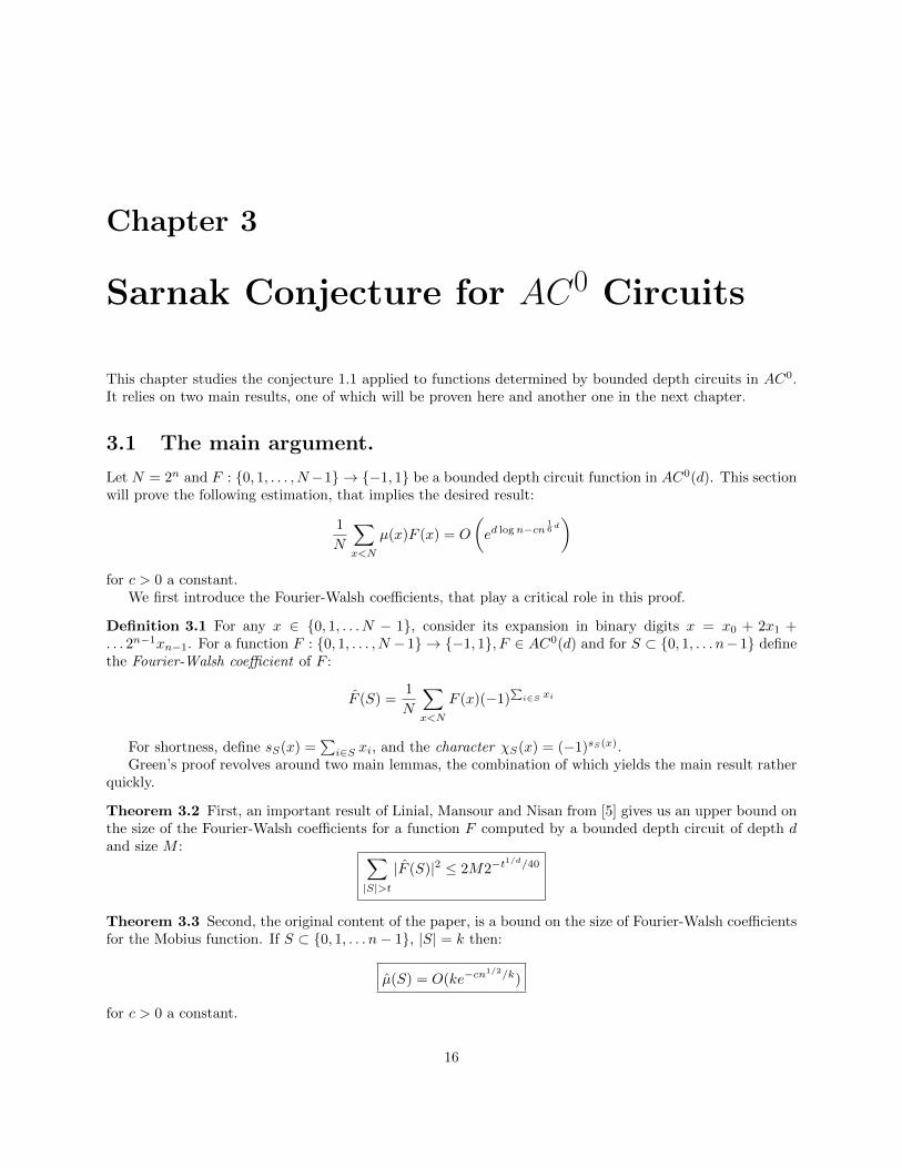
Chapter 3

Sarnak Conjecture for AC0 Circuits

This chapter studies the conjecture 1.1 applied to functions determined by bounded depth circuits in AC0.It relies on two main results, one of which will be proven here and another one in the next chapter.

3.1 The main argument.

Let N = 2n and F : {0, 1, . . . , N−1} → {−1, 1} be a bounded depth circuit function in AC0(d). This sectionwill prove the following estimation, that implies the desired result:

1

N

∑x<N

µ(x)F (x) = O

(ed logn−cn

16d

)for c > 0 a constant.

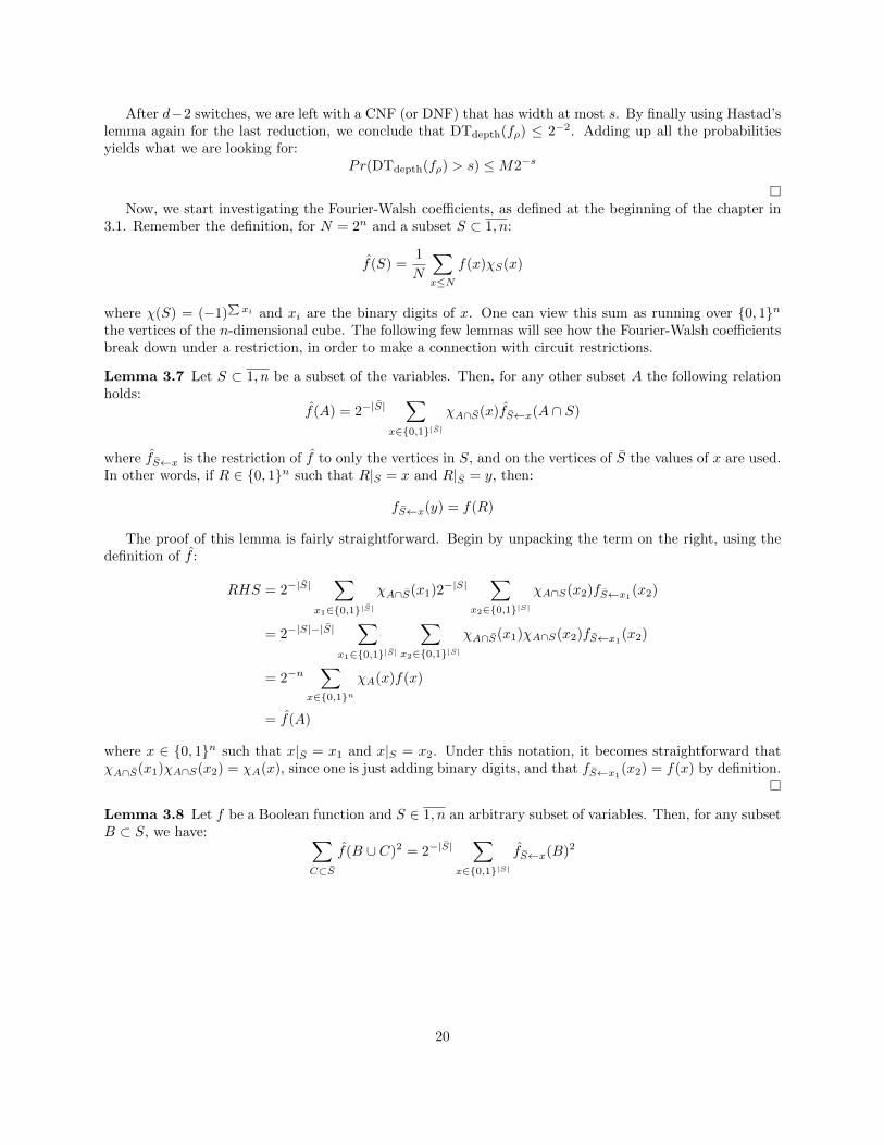
We first introduce the Fourier-Walsh coefficients, that play a critical role in this proof.

Definition 3.1 For any x ∈ {0, 1, . . . N − 1}, consider its expansion in binary digits x = x0 + 2x1 +. . . 2n−1xn−1. For a function F : {0, 1, . . . , N − 1} → {−1, 1}, F ∈ AC0(d) and for S ⊂ {0, 1, . . . n− 1} definethe Fourier-Walsh coefficient of F :

F (S) =1

N

∑x<N

F (x)(−1)∑i∈S xi

For shortness, define sS(x) =∑i∈S xi, and the character χS(x) = (−1)sS(x).

Green’s proof revolves around two main lemmas, the combination of which yields the main result ratherquickly.

Theorem 3.2 First, an important result of Linial, Mansour and Nisan from [5] gives us an upper bound onthe size of the Fourier-Walsh coefficients for a function F computed by a bounded depth circuit of depth dand size M : ∑

|S|>t

|F (S)|2 ≤ 2M2−t1/d/40

Theorem 3.3 Second, the original content of the paper, is a bound on the size of Fourier-Walsh coefficientsfor the Mobius function. If S ⊂ {0, 1, . . . n− 1}, |S| = k then:

µ(S) = O(ke−cn1/2/k)

for c > 0 a constant.

16

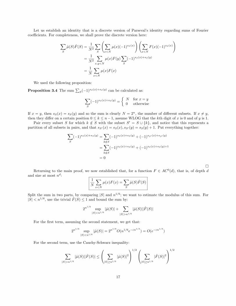
Let us establish an identity that is a discrete version of Parseval’s identity regarding sums of Fouriercoefficients. For completeness, we shall prove the discrete version here:

∑S

µ(S)F (S) =1

N2

∑S

(∑x<N

µ(x)(−1)sS(x)

)(∑x<N

F (x)(−1)sS(x)

)

=1

N2

∑x,y<N

µ(x)F (y)∑S

(−1)sS(x)+sS(y)

=1

N

∑x<N

µ(x)F (x)

We used the following proposition:

Proposition 3.4 The sum∑S(−1)sS(x)+sS(y) can be calculated as:

∑S

(−1)sS(x)+sS(y) =

{N for x = y0 otherwise

If x = y, then sS(x) = sS(y) and so the sum is clearly N = 2n, the number of different subsets. If x 6= y,then they differ on a certain position 0 ≤ k ≤ n− 1, assume WLOG that the kth digit of x is 0 and of y is 1.

Pair every subset S for which k /∈ S with the subset S′ = S ∪ {k}, and notice that this represents apartition of all subsets in pairs, and that sS′(x) = sS(x), sS′(y) = sS(y) + 1. Put everything together:∑

S

(−1)sS(x)+sS(y) =∑k/∈S

(−1)sS(x)+sS(y) + (−1)sS′ (x)+sS′ (y)

=∑k/∈S

(−1)sS(x)+sS(y) + (−1)sS(x)+sS(y)+1

= 0

�Returning to the main proof, we now established that, for a function F ∈ AC0(d), that is, of depth d

and size at most nd:1

N

∑x<N

µ(x)F (x) =∑S

µ(S)F (S)

Split the sum in two parts, by comparing |S| and n1/6; we want to estimate the modulus of this sum. For|S| < n1/6, use the trivial F (S) ≤ 1 and bound the sum by:

2n1/6

sup|S|<n1/6

|µ(S)|+∑

|S|>n1/6

|µ(S)||F (S)|

For the first term, assuming the second statement, we get that:

2n1/6

sup|S|<n1/6

|µ(S)| = 2n1/6

O(n1/6e−cn1/3

) = O(e−cn1/3

)

For the second term, use the Cauchy-Schwarz inequality:

∑|S|>n1/6

|µ(S)||F (S)| ≤

∑|S|≥n1/6

|µ(S)|21/2 ∑

|S|≥n1/6

|F (S)|21/2

17

The first sum can be estimated by using Parseval’s identity, in a very similar fashion to the one provedabove: ∑

|S|≥n1/6

|µ(S)|2 ≤∑S

µ(S) · µ(S) =1

N

∑x<N

µ(x)2 ≤ 1

and the second sum is estimated by assuming the first lemma 3.2:∑|S|≥n1/6

|F (S)|2 ≤ 2nd2−c′n1/6d

Putting everything together, we obtain the following upper bound:

1

N

∑x<N

µ(x)F (x) ≤ O(e−cn1/3

) +(

2nd2−c′n1/6d

)1/2

≤ O(ed logn−c′n1/6d

)≤ o(1)

as required, therefore proving the main result.

3.2 Linial, Mansour and Nisan result

An important tool in proving Theorem 3.2 will be Hastad’s Lemma 2.6, already discussed in the previouschapter. We restate it here.

Hastad’s Lemma. Let f be a DNF (or a CNF, by proposition 2.12) of width w and n variables, and ρ arandom restriction with parameter p = σn, σ ≤ 1/5. Then, for each parameter s:

Pr (DTdepth(fρ) > s) ≤ (10σw)s

and therefore, by the fact 2.11, we can write it as a CNF (or a DNF, respectively) with width smaller thans with a probability of at least 1 - (10σw)s. Furthermore, all clauses of this DNF have disjoint inputs.

Define the degree of a Boolean function as the size of the largest subset that does not kill f :

deg(f) = maxf(S) 6=0

|S|

and prove the following corollary of Hastad’s lemma regarding the degree of a Boolean function.

Corollary 3.5 For f a Boolean function, the following holds:

DTdepth(f) ≥ deg(f)

This takes a bit of insight to notice. Assume that this is not the case; that is, if DTdepth(f) = d there

exists a subset S, |S| > d such that f(S) 6= 0. Look at the decision tree of f , and let λ1, λ2, . . . , λk be therestrictions that they impose on the set of variables such that:

λ1 t λ2 t · · · t λk = {0, 1}n

Because DTdepth(f) = d, each λi fixes at most d variables. And because |S| > d, for each λi there exists

18

a variable xn(i) ∈ S, /∈ λi. Now, we can assert that f(S) = 0:

f(S) =1

N

∑x∈{0,1}n

f(x)χS(x)

=1

N

k∑i=1

∑x∈λi

f(x)χS(x)

=1

N

k∑i=1

∑x∈λi,xn(i)=0

f(x)χS(x)(1− 1) = 0

thus proving that DTdepth(f) ≥ deg(f).�

We shall use Hastad’s lemma repeatedly to prove the following lemma about circuits.

Lemma 3.6 Let f be a Boolean function computed by a circuit of size M and depth d. Then, if ρ is arandom restriction with parameter:

Pr (ρ(xi) = ∗) =1

20dsd−1

for some s, then:Pr (DTdepth(fρ) > s) ≤M2−s

View the circuit of f as stratified on d successive levels, each level with mi gates. Naturally,∑mi = M .

Also, view the random restriction ρ as a succession of random restrictions, the first one with parameter 1/20,and d− 1 successive ones with parameter 1/20s.

After the first restriction, with high probability, most of the gates from the lowest level will have at mosts inputs; of course, this step is needed to ensure the application of Hastad’s lemma to the further steps. Tosee this, for each gate on this level, consider two cases:

• If the original number of inputs is at least 2s, then the chances that this reduction kills it, that is, setsone of its inputs to 0 and is a and or to 1 and is a or, is at most:

0.5252s ≤ 2−s

• If the original number of inputs is at most 2s, then the probability that at least s inputs get assigneda ∗ is: (

2s

s

)20−s ≤ 2−s

Therefore, because there are m1 gates at this level, the probability of a failure is at most m12−s. Foreach successive step, the idea is to convert all CNFs into DNFs (or vice-versa) for the second and third layersfrom the bottom, so that they can be collapsed into a single level and thus reducing the depth of the entirecircuit.

By induction, we know that these gates composing the CNF (or DNF) have less than s inputs; or, inother words, width ≤ s. Therefore, when we switch it into a DNF (or CNF) under a random restriction withparameter p = 1/20s, by using Hastad’s switching lemma we know its probability to have width more thans:

Pr (DTdepth(fρ) > s) ≤(

101

20ss

)s= 2−s

This kind of switches lets us collapse the second and third levels above the input levels together, thusreducing the depth of the circuit by 1. The probability that this fails is at most mi2

−s, since for each gatethe probability is at most 2−s.

19

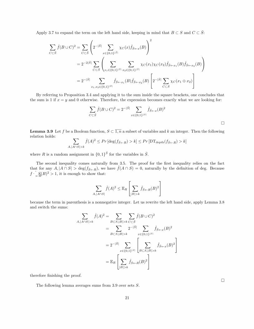
After d−2 switches, we are left with a CNF (or DNF) that has width at most s. By finally using Hastad’slemma again for the last reduction, we conclude that DTdepth(fρ) ≤ 2−2. Adding up all the probabilitiesyields what we are looking for:

Pr(DTdepth(fρ) > s) ≤M2−s

�Now, we start investigating the Fourier-Walsh coefficients, as defined at the beginning of the chapter in

3.1. Remember the definition, for N = 2n and a subset S ⊂ 1, n:

f(S) =1

N

∑x≤N

f(x)χS(x)

where χ(S) = (−1)∑xi and xi are the binary digits of x. One can view this sum as running over {0, 1}n

the vertices of the n-dimensional cube. The following few lemmas will see how the Fourier-Walsh coefficientsbreak down under a restriction, in order to make a connection with circuit restrictions.

Lemma 3.7 Let S ⊂ 1, n be a subset of the variables. Then, for any other subset A the following relationholds:

f(A) = 2−|S|∑

x∈{0,1}|S|χA∩S(x)fS←x(A ∩ S)

where fS←x is the restriction of f to only the vertices in S, and on the vertices of S the values of x are used.In other words, if R ∈ {0, 1}n such that R|S = x and R|S = y, then:

fS←x(y) = f(R)

The proof of this lemma is fairly straightforward. Begin by unpacking the term on the right, using thedefinition of f :

RHS = 2−|S|∑

x1∈{0,1}|S|χA∩S(x1)2−|S|

∑x2∈{0,1}|S|

χA∩S(x2)fS←x1(x2)

= 2−|S|−|S|∑

x1∈{0,1}|S|

∑x2∈{0,1}|S|

χA∩S(x1)χA∩S(x2)fS←x1(x2)

= 2−n∑

x∈{0,1}nχA(x)f(x)

= f(A)

where x ∈ {0, 1}n such that x|S = x1 and x|S = x2. Under this notation, it becomes straightforward thatχA∩S(x1)χA∩S(x2) = χA(x), since one is just adding binary digits, and that fS←x1

(x2) = f(x) by definition.�

Lemma 3.8 Let f be a Boolean function and S ∈ 1, n an arbitrary subset of variables. Then, for any subsetB ⊂ S, we have: ∑

C⊂S

f(B ∪ C)2 = 2−|S|∑

x∈{0,1}|S|fS←x(B)2

20

Apply 3.7 to expand the term on the left hand side, keeping in mind that B ⊂ S and C ⊂ S:

∑C⊂S

f(B ∪ C)2 =∑C⊂S

2−|S|∑

x∈{0,1}|S|χC(x)fS←x(B)

2

= 2−2|S|∑C⊂S

∑x1∈{0,1}|S|

∑x2∈{0,1}|S|

χC(x1)χC(x2)fS←x1(B)fS←x2

(B)

= 2−|S|

∑x1,x2∈{0,1}|S|

fS←x1(B)fS←x2

(B)

2−|S|∑C⊂S

χC(x1 ⊕ x2)

By referring to Proposition 3.4 and applying it to the sum inside the square brackets, one concludes that

the sum is 1 if x = y and 0 otherwise. Therefore, the expression becomes exactly what we are looking for:∑C⊂S

f(B ∪ C)2 = 2−|S|∑

x∈{0,1}|S|fS←x(B)2

�

Lemma 3.9 Let f be a Boolean function, S ⊂ 1, n a subset of variables and k an integer. Then the followingrelation holds: ∑

A,|A∩S|>k

f(A)2 ≤ Pr [deg(fS←R) > k] ≤ Pr [DTdepth(fS←R) > k]

where R is a random assignment in {0, 1}S for the variables in S.

The second inequality comes naturally from 3.5. The proof for the first inequality relies on the factthat for any A, |A ∩ S| > deg(fS←R), we have f(A ∩ S) = 0, naturally by the definition of deg. Because

ˆf ¯←RS(B)2 > 1, it is enough to show that:

∑A,|A∩S|

f(A)2 ≤ ER

∑|B|>k

fS←R(B)2

because the term in parenthesis is a nonnegative integer. Let us rewrite the left hand side, apply Lemma 3.8and switch the sums: ∑

A,|A∩S|>k

f(A)2 =∑

B⊂S,|B|>k

∑C⊂S

f(B ∪ C)2

=∑

B⊂S,|B|>k

2−|S|∑

x∈{0,1}|S|fS←x(B)2

= 2−|S|∑

x∈{0,1}|S|

∑B⊂S,|B|>k

fS←x(B)2

= ER

∑|B|>k

fS←R(B)2

therefore finishing the proof.

�The following lemma averages sums from 3.9 over sets S.

21

Lemma 3.10 Let f be a Boolean function, t an integer and 0 < p < 1. Then:

∑|A|>t

f(A)2 ≤ 2ES

∑|A∩S|>pt/2

f(A)2

where S ⊂ 1, n is randomly chosen, with each element having probability p to belong to S, and pt > 8.

Using a Chernoff bound, the probability for |A ∩ S| > pt/2 is larger than 1− exp(−pt/8) > 1/2. Therefore,each set A contributes with a probability of at least 1/2 for the sets on the left side, and the lemma is proven.

The proof for the bound used above will be presented now. Let A ⊂ 1, n be a fixed subset, |A| = t, andS ⊂ 1, n be a random subset, where each x ∈ 1, n has Pr(x ∈ S) = p for a parameter 0 < p < 1. Then:

Pr(|A ∩ S| > pt/2) > 1− exp(−pt/8)

Let A = {ai : 1 ≤ i ≤ n} and xi, 1 ≤ i ≤ n be random variables such that xi = 1 ⇐⇒ ai ∈ S, and 0otherwise. Let X =

∑xi; we want to evaluate Pr(X > pt/2).

The proof relies on applying Markov’s inequality to the exponential eλX for λ > 0. Recall Markov’sinequality:

Pr(X ≥ a) ≤ E(X)

a

and apply it as follows:

Pr(X ≤ pt/2) = Pr(e−λX ≥ e−λpt/2) ≤ eλpt/2E(e−λX)

≤ eλpt/2E(e−λxi)t

≤ eλpt/2(1 + p(e−λ − 1)

)t≤ eλpt/2ept(e

−λ−1)

≤ exp

(pt

(λ

2+ e−λ − 1

))Therefore, because λ > 0 is a parameter we can choose, pick for example λ = 1 and notice that:

λ

2+ e−λ − 1 = e−1 − 1

2= −0.13 ≤ −1

8

which proves the required relation.�

We are now ready to prove the main result 3.2. We shall restate it here:Lemma 3.2 For a function f computed by a bounded depth circuit of depth d and size M , the following

holds: ∑|S|>t

|f(S)|2 ≤ 2M2−t1/d/40

Fix p = 1/(20t(d−1)/d) and s = pt/2 = t1/d/40. By lemma 3.10, we know the following:

∑|A|>t

f(A)2 ≤ 2ES

∑|A∩S|>pt/2

f(A)2

with S ⊂ 1, n a random subset, where every element belongs to S with probability p.

Using lemma 3.9, we know the following bound:

2ES

∑|A∩S|>pt/2

f(A)2

≤ 2ESPr[DTdepth(fS←R) >

pt

2= s

]

22

The key observation now is that a selection of variables S randomly and uniformly with probability pand then a random association of {0, 1} values to S is exactly the same thing as a random restriction ρ withparameter p. Therefore, lemma 3.6 can be applied, because p = 1/(20dsd−1) and so we can conclude:∑

|A|>t

f(A)2 ≤ 2M2−s = 2M2−t1/d/40

thereby finishing the proof.

23

Chapter 4

Proof of Ben Green’s Relation

In this last chapter we prove the second required Lemma 3.3, following the argument presented in [3].Recall the statement of 3.3: If S ⊂ {0, 1, . . . n− 1}, |S| = k then:

µ(S) = O(ke−cn1/2/k)

for c > 0 a constant.The proof set forth by Ben Green in [3] begins by establishing a connection between the Fourier-Walsh

coefficients as defined above and the “traditional” Fourier coefficients:

F (θ) =1

N

∑x<N

F (x)e2iπxθ, θ ∈ [0, 1]

The first result we will prove is according to Katai.

Theorem 4.1 (Katai) Assume there exists a function F : {0, 1, . . . N − 1} → [−1, 1] such that there is asubset S ⊂ {0, 1, . . . n− 1}, |S| = k and the corresponding Fourier-Walsh coefficient |F (S)| > δ, 0 < δ < 1/2.Then there is a θ ∈ [0, 1] such that the Fourier coefficient |F (θ)| > (δ/10k)4k.

Moreover, this θ can be taken to be a sparse dyadic rational:

θ =r1

2i1+r2

2i2+ · · ·+ rk

2ik, ri ∈ Z, |ri| ≤ (10k/δ)3

4.1 Proof of Katai’s result

Define ψ : R/Z→ [−1, 1], an indicator function:

ψ(t) =

{1 if 0 ≤ t < 1

2−1 if 1

2 ≤ t < 1

and notice that we can rewrite sS(x) mod 2 as follows:

sS(x) =∑i∈S

xi ≡∏i∈S

ψ( x

2i

)because xi = 1 ⇐⇒ ψ(x/2i) = −1 and xi = 0 ⇐⇒ ψ(x/2i) = 1. Intuitively, both sums count theparity of the number of odd digits of x in binary form. This rewriting also translates into a rewriting of theFourier-Walsh coefficient:

F (S) =1

N

∑x<N

F (x)∏i∈S

ψ( x

2i

)

24

The main idea is to replace the function ψ by a function ψ that is both close enough to ψ and has areasonable Fourier expansion. Namely, we want the following two conditions to be satisfied, and we shallprove that such a function can be constructed through a smoothing procedure:

• Close to ψ, or, more specifically, for any 0 ≤ i ≤ n− 1:

1

N

∑x<N

∣∣∣ψ ( x2i

)− ψ

( x2i

)∣∣∣ ≤ ε• With a relatively well-behaved Fourier expansion:

ψ(t) =∑

r≤100ε−3

are2iπrt

such that |ar| ≤ 1 for all r.

First, we assume the above construction and present the remainder of the proof. Choose ε = δ/2k andreplace ψ with a ψ obtained through the above construction. Starting off with the original assumption,apply the triangle inequality repeatedly to achieve a lower bound for the Fourier coefficient:

|F (S)| = 1

N

∣∣∣∣∣∑x<N

F (x)∏i∈S

ψ( x

2i

)∣∣∣∣∣ ≥ δ1

N

∣∣∣∣∣∣∑x<N

F (x)(ψ( x

2i1

)+(ψ( x

2i1

)− ψ

( x

2i1

))) ∏i∈S,i 6=i1

ψ( x

2i

)∣∣∣∣∣∣ ≥ δ1

N

∣∣∣∣∣∣∑x<N

F (x)ψ( x

2i1

) ∏i∈S,i 6=i1

ψ( x

2i

)∣∣∣∣∣∣− ε

N

∣∣∣∣∣∣∑x<N

F (x)∏

i∈S,i 6=i1

ψ( x

2i

)∣∣∣∣∣∣ ≥ δSince F and ψ only take values between [−1, 1], the second sum is at most ε. Because |S| = k, this

procedure of extracting one ψ at a time will eventually yield:

1

N

∣∣∣∣∣∑x<N

F (x)∏i∈S

ψ( x

2i

)∣∣∣∣∣− kε ≥ δExpand every ψ in its Fourier series, and obtain:

1

N

∣∣∣∣∣∣∑x<N

F (x)∏i∈S

∑ri≤100ε−3

are2iπrix/2

i

∣∣∣∣∣∣ ≥ δ/21

N

∣∣∣∣∣∣∑x<N

F (x)∑

r1...rk<100ε−3

ar1 . . . ark exp

(2iπx

∑i∈S

ri2i

)∣∣∣∣∣∣ ≥ δ/2∣∣∣∣∣∣∑

r1...rk<100ε−3

ar1 . . . ark

(1

N

∑x<N

F (x) exp

(2iπx

∑i∈S

ri2i

))∣∣∣∣∣∣ ≥ δ/2∣∣∣∣∣∣∑

r1...rk<100ε−3

ar1 . . . ark F

(∑i∈S

ri2i

)∣∣∣∣∣∣ ≥ δ/2

25

One of the terms of this sum is greater than its average; therefore there exists a certain θ =∑i∈S

ri2i

such that:

ar1 . . . ark F (θ) ≥ δ

2

(ε3

100

)kUse |ari | < 1 and ε = δ/2k:

F (θ) ≥ δ

2

(δ3

200k

)k>

(δ

10k

)4k

which is the desired bound, and proves this part. The form of θ follows naturally from this construction.We now detail the construction of ψ as follows. First, consider a function ψ1 = φ ∗ χ ∗ χ, where

φ(t) = ψ(t+ ε/24), χ = 24/ε · 1[−ε/48,ε/48], for some ε > 0. The operator ∗ denotes the convolution operator,on the definition interval [0, 1]:

f ∗ g(t) =

∫ 1

0

f(τ)g(t− τ)dτ

Intuitively, this builds a continuous function that is close to ψ and can be further refined to fulfill allrequirements. More specifically, the reasons for this construction are as follows:

• ψ1 : R/Z→ [−1, 1]. This is natural, since ψ and χ are functions of period 1 with values in [−1, 1].

• ψ1 and ψ are the same almost everywhere, except on intervals whose length go to 0 as ε → 0. To seethis, look first at φ ∗ χ:

ψ1(t) = φ ∗ χ ∗ χ(t) =

∫ 1

0

χ(τ0)φ ∗ χ(t− τ0)dτ0

=24

ε

∫ ε/48

−ε/48

φ ∗ χ(t− τ0)dτ0

=24

ε

∫ ε/48

−ε/48

∫ 1

0

χ(τ1)φ(t− τ0 − τ1)dτ1dτ0

=

(24

ε

)2 ∫ ε/48

−ε/48

∫ ε/48

−ε/48

ψ(t− τ0 − τ1 − ε/24)dτ1dτ0

Recall that the function ψ is constant on the two intervals [0, 1/2] and [1/2, 1]. When the argumentof ψ is far away enough from the points 0 = 1 and 1/2, the function ψ1 ≡ ψ because of the aboverelation. Because −τ0 − τ1 − ε/24 ∈ [−ε/12, 0], this means that outside the intervals I1 = [ 1

2 −ε

12 ,12 ]

and I2 = [1− ε12 , 1] the functions ψ and ψ1 take the same values.

For any i, the rational numbers with denominator 2i are evenly distributed across the interval [0, 1],therefore conclude the following about the average value of the difference between ψ and ψ0:

1

N

∣∣∣ψ0

( x2i

)− ψ

( x2i

)∣∣∣ ≤ 2(|I1|+ |I2|) =ε

3

From the Fourier convolution theorem, the Fourier coefficients of ψ1 are given by ψ1(r) = φ(r)χ(r)2.Calculate the Fourier coefficients of χ directly:

χ(r) =

∫ 1

0

χ(r)e2iπxrdx

=24

ε

∫ ε/48

−ε/48

e2iπxrdx

=48

ε

∫ ε/48

0

cos(2πxr)dx = − 24

πrεsin(εxr/24)

26

Using the trivial bound on all Fourier coefficients φ, χ ≤ 1 deduce the bound:

|ψ1(r)| ≤ |χ(r)|2 ≤ min

(1,

24

πε|r|

)and use this bound to obtain another bound on:∑

r≥ 100ε3

|ψ1(r)| ≤∑r≥ 100

ε3

min

(1,

24

πε|r|

)2

≤(

24

πε

)2 ∑r≥ 100

ε3

1

r2

≤(

24

πε

)2π2

6<ε

3

Of course, this bound is useful because we wish to introduce ψ2(r) =∑r≤100/ε3 ψ1(r) exp(2iπrt). This

function is a truncation of the Fourier expansion of ψ1 which satisfies the requirement on its Fourier series,and is also close to ψ1 and implicitly to ψ:

maxr|ψ1(r)− ψ2(r)| ≤

∣∣∣∣∣∣∑

r>100/ε3

ψ1(r) exp(2iπrt)

∣∣∣∣∣∣ ≤ ε/3This function is almost what is required; the final function should take values in [−1, 1]. From the above

inequality, |ψ2(r)| ≤ ε/3 + 1, so introduce ψ = ψ2/(1 + ε/3). Again:

maxr|ψ(r)− ψ2(r)| ≤ max(ψ2)

(1

1 + ε/3

)≤ ε/3

and, finally, by the triangle inequality:

1

N

∑x<N

∣∣∣ψ ( x2i

)− ψ

( x2i

)∣∣∣ ≤ εtherefore proving that ψ is a function satisfying the requirements.

�By using this relation of Katai, an upper bound on the Fourier coefficients can be translated into another

upper bound on the Fourier-Walsh coefficient, for some subset S. Recall that we still needed to prove 3.3:

µ(S) = O(ke−cn1/2/k), for |S| = k

This bound is nontrivial for k = O(n1/2/ log n), therefore those are the interesting values that should beused with the Katai relation. Unfortunately, the existing bounds for µ do not yield the desired result, so wehave to rely on the specific sparse dyadic form of θ.

• Assuming the Generalized Riemann Hypothesis, one can deduce an upper bound µ(θ) �ε N−1/4+ε,

and this can be translated into a bound for µ(S), |S| = k.

By way of contradiction, assume that there exists subsets S of size k such that µ(S) 6= o(1) as n→∞,which means that µ(S) > δ a given constant. Therefore, by Katai’s relation, there exists θ ∈ [0, 1] such

27

that:

µ(θ) ≥(

δ

10k

)4k

2n(−1/4+ε) ≥(

δ

10k

)4k

n(−1/4 + ε) log 2 ≥ 4k log

(δ

10k

)n ≤ ck log k, for c > 0

c′n

log n≤ k, for c′ > 0

Therefore, under this assumption, the bound holds for k = O(n/ log n), which is more than enough toprove our point at hand.

• On the other hand, without assuming the GRH, the best known bound for µ(θ) is much higher,|µ(θ)| �A log−A(N), for any constant A > 0. This bound also leads to a bound on µ(S):

n−A log−A 2 ≥(

δ

10k

)4k

A(log n+ log log 2) ≤ 4k(log 10 + log k − log δ)

clog n

log log n≤ k, for c > 0

This bound for k is insufficient, smaller than the required k = O(n1/2).

4.2 Using the dyadic structure of θ

To make use of the structure of θ, we shall prove the following lemma:

Lemma 4.2 There exists a constant c with the following property: if k < n1/2, and:

θ =r1

2i1+ · · ·+ rk

2ikwith |ri| < exp(c log1/2N)

then:|µ(θ)| = O(exp(−c log1/2N))

We will show that this statement proves the main point 3.3. Suppose that there exists a subset S such

that |µ(S)| ≥ ke−cn1/2/k. Then by Katai’s relation, there exists a sparse dyadic θ r1

2i1+ · · · + rk

2ikfor which

|ri| � exp(3cn1/2/k) and |µ(θ)| ≥ exp(4cn1/2/k). Replace N = 2n in the statement’s relation and choose csmall enough so that a contradiction appears.

�Returning to the proof of Lemma 4.2, we shall use the following theorem:

Theorem 4.3 Let µ be the Mobius character, and consider the Dirichlet characters χ to modulus q = 2t ≤exp(c1 log1/2N). Then:

1

N

(∑x<N

µ(x)χ(x)

)= O(exp(−c1 log1/2N))

28

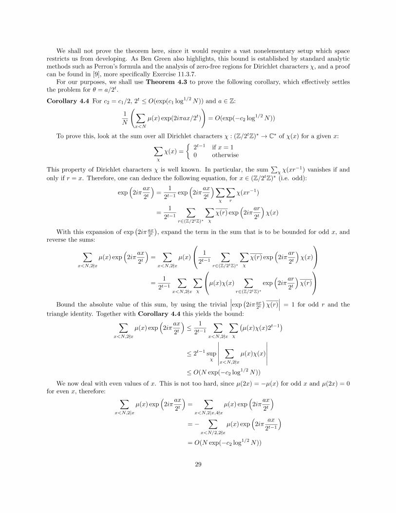
We shall not prove the theorem here, since it would require a vast nonelementary setup which spacerestricts us from developing. As Ben Green also highlights, this bound is established by standard analyticmethods such as Perron’s formula and the analysis of zero-free regions for Dirichlet characters χ, and a proofcan be found in [9], more specifically Exercise 11.3.7.

For our purposes, we shall use Theorem 4.3 to prove the following corollary, which effectively settlesthe problem for θ = a/2t.

Corollary 4.4 For c2 = c1/2, 2t ≤ O(exp(c1 log1/2N)) and a ∈ Z:

1

N

(∑x<N

µ(x) exp(2iπax/2t)

)= O(exp(−c2 log1/2N))

To prove this, look at the sum over all Dirichlet characters χ : (Z/2tZ)∗ → C∗ of χ(x) for a given x:∑χ

χ(x) =

{2t−1 if x = 10 otherwise

This property of Dirichlet characters χ is well known. In particular, the sum∑χ χ(xr−1) vanishes if and

only if r = x. Therefore, one can deduce the following equation, for x ∈ (Z/2tZ)∗ (i.e. odd):

exp(

2iπax

2t

)=

1

2t−1exp

(2iπ

ax

2t

)∑χ

∑r

χ(xr−1)

=1

2t−1

∑r∈(Z/2tZ)∗

∑χ

χ(r) exp(

2iπar

2t

)χ(x)

With this expansion of exp(2iπ ax2t

), expand the term in the sum that is to be bounded for odd x, and

reverse the sums:∑x<N,2-x

µ(x) exp(

2iπax

2t

)=

∑x<N,2-x

µ(x)

1

2t−1

∑r∈(Z/2tZ)∗

∑χ

χ(r) exp(

2iπar

2t

)χ(x)

=

1

2t−1

∑x<N,2-x

∑χ

µ(x)χ(x)∑

r∈(Z/2tZ)∗

exp(

2iπar

2t

)χ(r)

Bound the absolute value of this sum, by using the trivial

∣∣∣exp(2iπ ar2t

)χ(r)

∣∣∣ = 1 for odd r and the

triangle identity. Together with Corollary 4.4 this yields the bound:∑x<N,2-x

µ(x) exp(

2iπax

2t

)≤ 1

2t−1

∑x<N,2-x

∑χ

(µ(x)χ(x)2t−1

)

≤ 2t−1 supχ

∣∣∣∣∣∣∑

x<N,2-x

µ(x)χ(x)

∣∣∣∣∣∣≤ O(N exp(−c2 log1/2N))

We now deal with even values of x. This is not too hard, since µ(2x) = −µ(x) for odd x and µ(2x) = 0for even x, therefore: ∑

x<N,2|x

µ(x) exp(

2iπax

2t

)=

∑x<N,2|x,4-x

µ(x) exp(

2iπax

2t

)= −

∑x<N/2,2-x

µ(x) exp(

2iπax

2t−1

)= O(N exp(−c2 log1/2N))

29

Add the bounds for the two sums and arrive at the proof of the corollary.�

The next corollary proves the problem for θ close to a number of the form a/2t.

Corollary 4.5 Let c3 = c2/3 and q = 2t ≤ exp(c3 log1/2N). If |θ − a/q| ≤ exp(c3 log1/2N)/N , then:

µ(θ) = O(exp(−c3 log1/2N))

The main idea behind proving this corollary is approximating θ with a/q in the sum µ(θ) =∑x<N µ(x)e2iπθx,

after splitting up the interval [1, N ] in N/L intervals of size L, where L is to be determined. For such aninterval I of length L and for x0 ∈ I, estimate:∣∣∣∣∣∑x∈I

µ(x) exp(2iπxθ)

∣∣∣∣∣ =

∣∣∣∣∣exp(2iπx0(θ − a/q))∑x∈I

µ(x) exp

(2iπ

ax

q

)exp(2iπ(x− x0)(θ − a/q))

∣∣∣∣∣≤

∣∣∣∣∣∑x∈I

µ(x) exp

(2iπ

ax

q

)∣∣∣∣∣+

∣∣∣∣∣∑x∈I

µ(x) exp

(2iπ

ax

q

)(exp(2iπ(x− x0)(θ − a/q))− 1)

∣∣∣∣∣≤ O(N exp(−c2 log1/2N)) +

∑x∈I|2iπ(x− x0)(θ − a/q)|

≤ O(N exp(−c2 log1/2N)) + LO(L exp(c3 log1/2N)/N)

Therefore, the entire sum can be bounded by bounding on each of the N/L intervals:

µ(θ) =1

N

(∑x<N

µ(x) exp(2iπxθ)

)

=1

N

N

LO(N exp(−c2 log1/2N))

1

N

N

LLO(L exp(c3 log1/2N)/N)

= O

(N

Lexp(−c2 log1/2N)

)+O

(L

Nexp(c3 log1/2N)

)Choose a suitable L = N exp(−2c3 log1/2N) such that the bound is O

(exp(−c3 log1/2N)

), therefore proving

the second corollary.�

The next corollary provides a good estimation for µ(θ) when θ is close to a rational number with arelatively small denominator that is a power of 2. We shall state and prove a bound for µ(θ) when θ is notapproximated by any rational number with a small denominator; this be useful later on.

Corollary 4.6 Suppose |µ(θ)| ≥ δ. Then there exists q � (logN/δ)16 such that:

|θ − a/q| � (logN/δ)16N−1

To prove this, choose Q = c(logN/δ)−16N for c > 0 to be determined. Use the Dirichlet diophantineapproximation theorem to conclude that there exists a, q, 1 ≤ q ≤ Q such that:∣∣∣∣θ − a

q

∣∣∣∣ ≤ 1

qQ≤ 1

q2

For such a θ, theorem 13.9 from Iwaniec and Kowalski [6] proves a bound for µ(θ):

N |µ(θ)| �(q1/2N1/2 + q−1/2N +N4/5

)1/2

N1/2(logN)4

δ(logN)−4 � max(q1/4N−1/4, q−1/4, N−1/10

)Consider each of the three cases and establish the required bound.

30

• If δ(logN)−4 � q1/4N−1/4, then, because q ≤ Q = c(logN/δ)−16N :

δ � (logN)4N−1/4c1/4(logN/δ)−4N1/4

δ5 � c1/4

which does not hold if c is small enough.

• If δ(logN)−4 � q−1/4, then

q � logN

δ

as required, and the proof is over.

• If δ(logN)−4 � N−1/10, then, for example, δ � N1/16 and the bound is trivially achieved, because:

(logN/δ)16N−1 � (logN)16N−1N � 1 ≥ |θ − a/q|

�This result provides a bound for values of θ that are far from rationals with small denominators, and

Corollary 4.6 takes care of θ that are close to dyadic numbers. We shall prove that there are no sparsedyadic numbers that do not fall into one of these categories, and this will imply the final result.

Lemma 4.7 Let θ =∑kt=1

rt2it

be a sparse dyadic number, such that i1 < i2 < · · · < ik ≤ n and |ri| ≤ Q.

Suppose furthermore that |θ − a/q| ≤ Q/N for some q ≤ Q, (a, q) = 1 and that 2n/2k ≥ 4Q2. Then q is apower of two.

Denote i0 = 0, ik+1 = n, and observe that:

n =

k∑t=0

it+1 − it

Among these k gaps, there has to be a largest one, that is, there is a j such that ij+1 − ij ≥ n/2k.Therefore, θ is close to the sum of its first j terms; more specifically, consider q′ = 2j and a′ = r12ij−i1 +· · ·+ rj−12ij−ij−1 + rj . The partial geometric sum can be approximated:

|Q− a′

q′| ≤ Q(2ij+1 + 2ij+2 + · · ·+ 2ik) ≤ 21−n/2kQ

q′

Use that q′ ≤ 2n − n/2k and therefore Q/N ≤ 1/4Qq′. The final bound:∣∣∣∣aq − a′

q′

∣∣∣∣ ≤ ∣∣∣∣θ − a′

q′

∣∣∣∣+

∣∣∣∣θ − a

q

∣∣∣∣≤ 21−n/2kQ

q′+Q

N

≤ 1

2Qq′+

1

4Qq′≤ 1

Qq′

≤ 1

qq′

therefore a = a′, q = q′.�

We are now ready to complete the proof of the main statement 4.2. Recall the statement, there exists aconstant c with the following property: if k < n1/2, and:

θ =r1

2i1+ · · ·+ rk

2ikwith |ri| < exp(c log1/2N)

31

then:|µ(θ)| = O(exp(−c log1/2N))

Suppose δ = exp(−c log1/2N) such that there exists θ for which |µ(θ)| ≥ δ. According to the result we

proved above, there exists q ≤(

logNδ

)16

such that the bound holds:

∣∣∣∣θ − a

q

∣∣∣∣ ≤ ( logN

δ

)16

N−1

Because δ � 1/ logN , we can rewrite that as:∣∣∣∣θ − a

q

∣∣∣∣ ≤ exp

(−c log1/2N

32

)N−1

Now, apply the previous lemma for Q = c log1/2 N32 and check that all conditions are satisfied. Indeed, |ri| ≤ Q

trivially by hypothesis, and 2n/2k ≥ 4Q2 as well, so q is a power of two.Then, by the result we proved above, we get µ(θ) = O(exp(−c2 log1/2N)), thereby finishing the proof.

32

Bibliography

[1] Sarnak, P., 2011. Three lectures on the Mobius function, randomness and dynamics. Institute for AdvancedStudy, New Yersey.

[2] Tao T., 2012. The Chowla conjecture and the Sarnak conjecture. Unpublished. https://terrytao.

wordpress.com/2012/10/14/the-chowla-conjecture-and-the-sarnak-conjecture/

[3] Green, B, (2012). On (Not) Computing the Mobius Function Using Bounded Depth Circuits. Combina-torics, Probability & Computing, 21(6), 942-951.

[4] Bender, E.A. and Goldman, J.R., 1975. On the applications of Mobius inversion in combinatorial analysis.American Mathematical Monthly, pp.789-803.

[5] Linial, N., Mansour, Y. and Nisan, N., 1993. Constant depth circuits, Fourier transform, and learnability.Journal of the ACM (JACM), 40(3), pp.607-620.

[6] Iwaniec, H., Kowalski, E. 2004. Analytic Number Theory, ISBN-10: 0-8218-3633-1, ISBN-13: 978-0-8218-3633-0, Colloquium Publications, vol. 53

[7] Hastad, J., 1986. Almost optimal lower bounds for small depth circuits. Proceedings of the eighteenthannual ACM symposium on Theory of computing. ACM.

[8] Razborov, A.A., 1985. A lower bound on the monotone network complexity of the logical permanent.Math. Zametki 37, (1985b) 887-900 (Russian) [English transl.: Math. Notes of the Acad. Sci. USSR37(6) 485-493]

[9] Montgomery H.L., Vaughan R.C., 2006. Multiplicative Number Theory I. Classical Theory ISBN-13 978-0-511-25746-9

[10] Pinsky, R.G., 2014. Problems from the Discrete to the Continuous, Universitext, DOI 10.1007/978-3-319-07965-3 2, Springer International Publishing Switzerland

[11] Peckner, R., 2015. Uniqueness of the measure of maximal entropy for the squarefree flow, Israel Journalof Mathematics September 2015, Volume 210, Issue 1, pp 335-357

[12] Stuhlsatz, E., 2015 Mobius Inversion Formula, Unpublished, https://www.whitman.edu/Documents/Academics/Mathematics/stuhlsatz.pdf

33