1

THE ROLE OF SALIENCE AND ATTENTION IN CHOICE UNDER RISK:

AN EXPERIMENTAL INVESTIGATION

Cary Frydman and Milica Mormann*

July 2017

ABSTRACT: We conduct three experiments, using a combination of lottery choices and eyetracking data, to test a recently proposed theory of choice under risk called salience theory. In our first experiment, subjects choose between risky lotteries and we manipulate the salience of payoffs by varying the correlation between lotteries. Risk taking decreases systematically with correlation, which is consistent with salience theory, but is inconsistent with expected utility and prospect theory. In our second experiment, we use eyetracking data to test the psychological mechanism. Subjects choose between a risky lottery and a certain option, and we find that attention to the risky lottery’s upside correlates with the probability of taking risk. In our final experiment we establish that there is a causal, but asymmetric, impact of attention on risky choice. While no single piece of evidence is decisive, salience theory offers a parsimonious explanation for the broad set of experimental results.

* Frydman is at the Department of Finance and Business Economics, USC Marshall School of Business, cfrydman@marshall.usc.edu; Mormann is at the Department of Marketing, SMU Edwin L. Cox School of Business, mmormann@cox.smu.edu. We are thankful for comments and suggestions from Kenneth Ahern, Nicholas Barberis, Pedro Bordalo, Ben Bushong, Tom Chang, Nicola Gennaioli, Lawrence Jin, Chad Kendall, Ian Krajbich, Jon Leland, Salvatore Nunnari, Andrei Shleifer, Ryan Webb, and from seminar participants at Caltech, Columbia University, Harvard University, Maastricht University, New York University, UCLA, University of Mannheim, University of Miami, University of Southern California, the UBS and University of Zurich Conference on Behavioral Finance, Society for Neuroeconomics Conference, and Southern California Finance Conference.

2

1. INTRODUCTION

A key tenet of expected utility theory is that preferences are stable over time and are independent

of the context in which choices are presented. However, starting with Allais (1953), a large body

of evidence documents robust violations of context-independent choice. One potential mechanism

that can generate context dependence is attention, which “refers to the brain’s ability to vary the

resources that it deploys in different circumstances” (Fehr and Rangel 2011, pg. 13). In one

circumstance, a bright red object in a black painting may capture attention, while this same bright

red object may not capture attention in a different circumstance where it does not appear unusual

(e.g., if the entire painting is also red). While these principles of visual attention have been well

studied for decades (Itti and Koch 2001), they have only recently been applied to economic

decision-making.

Bordalo, Genniaoli, Shleifer (2012) (henceforth BGS) provide the first behavioral

economic model, called salience theory, that uses principles from visual attention to explain

economic choice under risk. To illustrate the psychology of the model, consider a decision-maker

presented with a choice between a positively skewed lottery and a mean preserving certain

option. The decision maker’s attention is attracted to the state where the risky lottery delivers a

high payoff because this payoff is very different from the average payoff, and it is thus salient.

Attention is drawn to the salient high payoff state, and this state is overweighed in the decision

making process, which induces risk taking. This example illustrates the general relationship that

salience theory establishes: precisely defined salient payoffs attract attention, and this attention

allocation systematically influences risk preferences. While salience theory can provide a unified

explanation for several features and anomalies of choice under risk, the theory has not yet been

directly tested.

In this paper, we test salience theory by conducting a series of experiments that combine

data on risky choice with direct measures of attention. The experiments are carefully designed to

overcome two significant challenges in testing salience theory. The first challenge is

3

manipulating the salience of a payoff in a manner that does not affect predictions under

alternative theories of choice under risk. The second challenge is obtaining direct measures of

attention during the decision-making process. We optimize the design of each of our three

experiments to overcome a different aspect of these challenges in testing the theory. The full

details of each experiment are presented in the main body of the paper, but we briefly summarize

the key design features and results here.

Our first experiment is designed to separate salience theory from competing theories of

choice under risk, including expected utility and cumulative prospect theory (CPT) (Kahneman

and Tversky 1992). The challenge here is that manipulating the salience of a payoff will often

affect the utility of the payoff under alternative theories, thus making it difficult to isolate the

effect of salience on risk taking. To overcome this challenge, we design the experiment to test a

strong prediction of salience theory, which states that the correlation between (mutually

exclusive) lotteries affects risk-taking, even as the marginal distribution of each lottery remains

constant. The intuition is that correlation changes the probability of each state, and the salience of

a lottery payoff is determined by payoff comparisons within a state; therefore, by shifting the

correlation, this will change the decision-maker’s perception of risk even if the marginal

distribution of each lottery remains constant.

To test this prediction, we ask subjects to choose between two lotteries that are typically

presented in experiments on the Allais paradox. Using a within subjects design, we

experimentally manipulate the correlation across different choice sets, while holding the marginal

payoff distribution of each lottery constant. Therefore, under both expected utility and CPT, risk

taking should not vary with correlation. We find that correlation does systematically impact risk

taking in the manner predicted by BGS, as the propensity to exhibit the Allais paradox

monotonically decreases in the correlation between lotteries. While these data are consistent with

salience theory, this experiment does not allow us to rule out an alternative theory of choice under

risk: regret theory (Loomes and Sugden 1982; Bell 1982). Regret theory operates through a

4

fundamentally different psychological mechanism, and we therefore design a second experiment

to directly test the underlying psychological mechanism.

In our second experiment, we test whether attention is associated with risk taking through

the mechanism proposed in salience theory. The challenge in conducting this test is obtaining

measures of attention during the decision-making process. We address this by directly measuring

attention with eyetracking data while subjects make a series of lottery choices between a risky

lottery and a certain option. On each trial, there is one state where the risky lottery delivers a gain

relative to the certain option – the gain state – and another state where the risky lottery delivers a

loss – the loss state.

We find that attention does correlate with risky choice in the manner proposed by BGS.

The amount of time a subject looks at the gain state relative to the loss state is positively

correlated with the probability of choosing the risky lottery. This correlation remains significant

after controlling for choice set fixed effects, which indicates that individual differences in

attention can explain variation in risk taking across subjects. These results therefore provide novel

empirical evidence for a connection between attention and risk taking, and this connection is

consistent with the state-based attention mechanism proposed in salience theory. At the same

time, our results raise an important question about the direction of causality. Under salience

theory, attention causally affects risk preferences, but the eyetracking data cannot rule out the

possibility that stable risk preferences causally affect attention allocation.

In order to test for causality, we conduct a third and final experiment in which we

experimentally manipulate the visual salience of a choice set. We exogenously shift attention

through the visual properties (e.g., color and transparency) of a lottery payoff, while holding

constant the magnitudes of payoffs and probabilities for each lottery in the choice set. This allows

us to test for a causal impact of attention on risky choice.

When we increase the visual salience of the risky lottery’s downside, which makes the

loss state “pop out,” subjects become more risk averse and choose the risky lottery less often than

5

in the control condition. In a separate treatment, we increase the visual salience of the risky

lottery’s upside, but we find no significant difference in risk taking compared to the control

condition. The results from our final experiment indicate that there is a causal, but asymmetric

impact, of attention on risky choice.

When taken together, the results from our three experiments demonstrate that salience

and attention are important factors in explaining choice under risk. We find that manipulating the

correlation between risky lotteries in a manner that renders a risky lottery’s upside or downside

salient has an impact on choice in the direction predicted by salience theory. The eyetracking data

then provide support for the psychological mechanism, whereby greater attention to a risky

lottery’s upside is associated with greater risk taking. Our visual salience manipulation provides

evidence that attention has a causal impact on risk taking. While no single piece of evidence is

decisive, salience theory offers a parsimonious explanation for the set of results across our three

experiments.

The experiments in this paper are designed specifically to test salience theory, but they

are more broadly related to a recent surge of economic theory on endogenous attention allocation

and choice1. Koszegi and Szeidl (2013) provide a model where agents focus on attributes that are

most different across alternatives and subsequently overweigh these attributes at the time of

choice. Schwartzstein (2014) studies an agent whose selective attention leads to biased belief

updating and Gabaix (2014) builds a general and tractable theory of an agent who chooses

attention weights to build a “sparse” model of the world. Cunningham (2013) and Bushong,

Rabin, and Schwartzstein (2016) provide related formal models where the choice set

endogenously influences decision weights. Salience theory has also been applied and tested in the

setting of deterministic consumer choice (Bordalo, Genniaoli, Shleifer 2013; Dertwinkel-Kalt et

1 Our work is also related to earlier models by Rubinstein (1988) and Leland (1994) who propose theories of context-dependent choice under risk, though the psychology of these models is not explicitly motivated by attention.

6

al. 2016). As this theoretical literature continues to grow, some of our experimental results may

prove useful in guiding future model development among this class of theories.

Finally, our paper is also related to a growing experimental literature in decision

neuroscience that studies mechanisms that are common to economic and perceptual decision-

making (Summerfield and Tsetsos 2012; Towal, Mormann, and Koch 2013; Frydman and Nave

2016). For example, the drift diffusion model has been used for decades in psychophysics to

jointly model choices and response time during perceptual decision-making (Ratcliff 1978), and

recent work has shown that the same decision processes are in part responsible for simple

economic choice (Krajbich, Armel, and Rangel 2010; Milosavljevic et al. 2010). We contribute to

this literature by demonstrating that mechanisms from sensory perception can also be used to

explain choice under risk.

2. SALIENCE MODEL OF CHOICE UNDER RISK

In this section we present the BGS model of a decision maker (DM) faced with a choice

set that consists of two lotteries, {𝐿!, 𝐿!}. The lotteries are defined over a state space 𝑆 that

contains 𝑁 states. Each state 𝑠 ∈ 𝑆 occurs with probability 𝑝!, and lottery 𝐿! delivers payoff 𝑥!! in

state 𝑠. We assume the DM uses a linear value function 𝑣 𝑥 = 𝑥, where lottery payoffs are

evaluated relative to a reference point of zero. Without any salience distortions, the value of

lottery 𝐿! is given by:

𝑉 𝐿! = 𝑝!!∈! 𝑣 𝑥!! (1)

The salience model departs from this valuation equation by assuming that the DM does not use

the set of objective probabilities {𝑝!}, but instead uses a set of decision weights, 𝜔! . The

decision weights 𝜔! are a function of the salience of lottery payoffs and state probabilities.

7

The salience of a lottery payoff is defined by a continuous and bounded function that

maps payoffs into a salience measure. The function satisfies two properties: ordering and

diminishing sensitivity. Under ordering, the salience of a state is higher when payoff levels within

the state are further from a reference level; under diminishing sensitivity, salience decreases as

payoff levels rise. Formally, suppose there are two states 𝑠 and 𝑠′. Ordering implies that if

[𝑥!!, 𝑥!!] is a subset of [𝑥!! ! , 𝑥!!! ] then state 𝑠! is more salient than state 𝑠. Diminishing sensitivity

implies that if 𝑥!! > 0 and 𝑥!! > 0, then for any 𝜖 > 0, state s becomes less salient if 𝜖 is added to

payoffs 𝑥!! and 𝑥!!. For most of the paper, we work with a general salience function that need only

satisfy ordering and diminishing sensitivity. However, to generate some of the predictions in our

eyetracking experiment, we will use a specific salience function given by:

𝜎 𝑥!!, 𝑥!! = !!!!!!!

!!|!!! ! |!!!, (2)

where 𝜃 > 0. In this specific function, the numerator encodes the ordering property while the

denominator encodes the diminishing sensitivity property; as 𝜃 gets larger, the degree of

diminishing sensitivity decreases.

The salience measure of state s, for a general salience function, 𝜎 𝑥!!, 𝑥!! , is used to

distort the objective probability into a decision weight, 𝜔!. Specifically, for any two states 𝑠 and

𝑠!, the objective odds ratio !!!!!

, is distorted into a distorted odds ratio, !!!!!

, given by:

!!!!!

= ! ! !!!! , !!!

!

! ! !!!, !!!× !!!!!

. (3)

We then normalize the distorted probabilities such that they sum to one, which generates a unique

set of decision weights given by 𝜔! = !!!!!∈!

. In equation (3), the parameter 𝛿 ∈ 0,1

8

captures the degree to which salience distorts objective probabilities, where this distortion is a

smooth increasing function of the difference in salience across states2. When 𝛿 = 1, there is no

probability distortion and 𝑝! = 𝜔! for all 𝑠. The value of lottery 𝐿! under the BGS model can be

written as:

𝑉 𝐿! = 𝜔!!∈! 𝑣 𝑥!! (4)

We define the decision value of choosing 𝐿! from {𝐿!, 𝐿!} as the difference in lottery

values: 𝐷𝑉!! = 𝑉 𝐿! − 𝑉 𝐿! . Finally, in order to map 𝐷𝑉!! into choices, we assume that

choices are stochastic where the value of each lottery, 𝑉 𝐿! , is subject to an independent and

additive random shock3. The probability of choosing 𝐿! is therefore strictly increasing in 𝑉 𝐿!

and strictly decreasing in 𝑉 𝐿! .

3. EXPERIMENT ONE: CORRELATED ALLAIS PARADOX

In our first experiment, subjects are asked to choose between lotteries that are typically

used in Allais paradox experiments. The experiment is designed to exploit a strong prediction of

salience theory, which states that the correlation between lotteries has an impact on risk taking,

even while holding the marginal distribution of each lottery constant. Importantly, this prediction

is not shared by expected utility or CPT. We derive the theoretical predictions, describe the

experimental procedures, and then present the results.

2 In the original BGS model, the distortion is generated by the difference in salience rankings, but here we use the difference in salience values in order to avoid discontinuities in valuation. 3 For a review of the literature on stochastic binary choice over lotteries, see Wilcox (2008). The theoretical foundation of stochastic choice is an active area of research. Besides the random utility model interpretation, other theories of stochastic choice include deliberate randomization (Fudenberg, Iijima, and Strzalecki (2015); Agranov and Ortoleva (2017)) and bounded rationality, which can be derived from neurobiological constraints on the choice process (Fehr and Rangel (2011); Webb (2015); Woodford (2016), Khaw, Li, and Woodford (2017)).

9

3.1 Theoretical predictions for behavior

To begin, consider a DM who faces a choice set of lotteries given by {𝐴! 𝑧 , 𝐴! 𝑧 },

where the two lotteries are characterized by the following marginal payoff distributions:

𝐴! 𝑧 = 25, 0.33; 0, 0.01; 𝑧, 0.66

𝐴! 𝑧 = 24, 0.34; 𝑧, 0.66 (5)

The parameter 𝑧 ∈ {0, 24} is a common consequence, and in standard Allais paradox

experiments, subjects are asked to make choices as this common consequence varies. The classic

result is that subjects choose 𝐴! 0 and 𝐴! 24 , reversing their choice as a function of the

common consequence. This behavior violates the independence axiom and generates the Allais

paradox.

3.1.1 The case of z=0

In order to derive the predictions that BGS make about the Allais paradox, we need to

first define the state space. We begin with the case where the common consequence 𝑧 equals zero.

The choice set {𝐴! 0 , 𝐴! 0 } only characterizes the marginal distribution of each lottery, but we

can also characterize the joint distribution by adding an additional parameter, 𝛽 ∈ [!!, 1]. The

joint distribution of the two lotteries is given in Table 1, where columns represent states and rows

represent lotteries. We show in the Appendix that the correlation between lotteries is a linear and

increasing function of 𝛽. At the same time, the marginal distribution of each lottery does not

change with 𝛽, and therefore the predictions of CPT and expected utility will not vary with 𝛽.

To see how correlation affects risk taking under BGS, we first compute the decision

value of choosing 𝐴!(0) as a function of 𝛽, which we denote by 𝐷𝑉!!(!)! . Using the decision value

definition, we can write:

10

𝐷𝑉!!(!)! = 𝜔! 𝛽 × 𝑣 𝑥!!

! − 𝑣 𝑥!!!

!∈!

= 𝜔!(𝛽)×(!∈!

𝑥!!! − 𝑥!!

!)

= 𝜔!! 𝛽 0 − 0 + 𝜔!! 𝛽 25 − 0 + 𝜔!! 𝛽 0 − 24 + 𝜔!! 𝛽 25 − 24

= 25𝜔!! 𝛽 −24𝜔!! 𝛽 + 𝜔!! 𝛽 (6)

Because the decision weights are a function of parameters 𝛿 and 𝜎, (equation (3)), the

decision value will also depend on these parameters. We prove in the Appendix that for all

parameter values and salience functions, there is a monotonic relationship between the decision

value and 𝛽. The following proposition characterizes this relationship:

Proposition 1: For any salience function, and for all 𝛿 ∈ (0,1), the decision value of choosing

lottery 𝐴!(0) is strictly decreasing in 𝛽.

Using this result, it is straightforward to derive the relationship between risk taking and

correlation. First, since correlation is linearly increasing in 𝛽, then the decision value must be

strictly decreasing in correlation. Second, because the probability of choosing 𝐴!(0) is strictly

increasing in the decision value (through the stochastic choice function), it follows that the

probability of choosing 𝐴! 0 , is decreasing in correlation. This is summarized in the following

corollary.

Corollary 1: For any salience function, and for all 𝛿 ∈ (0,1), the probability of choosing 𝐴!(0) is

strictly decreasing in the correlation between 𝐴!(0) and 𝐴! 0 .

11

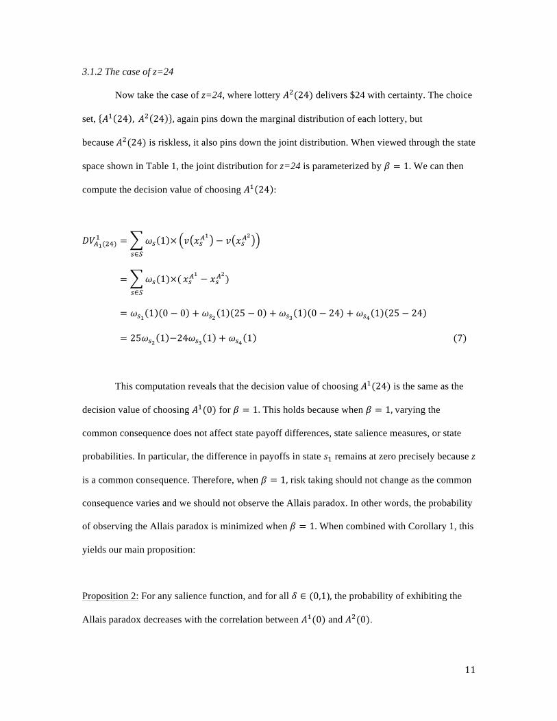
3.1.2 The case of z=24

Now take the case of z=24, where lottery 𝐴!(24) delivers $24 with certainty. The choice

set, 𝐴! 24 , 𝐴! 24 , again pins down the marginal distribution of each lottery, but

because 𝐴!(24) is riskless, it also pins down the joint distribution. When viewed through the state

space shown in Table 1, the joint distribution for z=24 is parameterized by 𝛽 = 1. We can then

compute the decision value of choosing 𝐴! 24 :

𝐷𝑉!!(!")! = 𝜔! 1 × 𝑣 𝑥!!

! − 𝑣 𝑥!!!

!∈!

= 𝜔!(1)×(!∈!

𝑥!!! − 𝑥!!

!)

= 𝜔!! 1 0 − 0 + 𝜔!! 1 25 − 0 + 𝜔!! 1 0 − 24 + 𝜔!! 1 25 − 24

= 25𝜔!! 1 −24𝜔!! 1 + 𝜔!! 1 (7)

This computation reveals that the decision value of choosing 𝐴!(24) is the same as the

decision value of choosing 𝐴!(0) for 𝛽 = 1. This holds because when 𝛽 = 1, varying the

common consequence does not affect state payoff differences, state salience measures, or state

probabilities. In particular, the difference in payoffs in state 𝑠! remains at zero precisely because z

is a common consequence. Therefore, when 𝛽 = 1, risk taking should not change as the common

consequence varies and we should not observe the Allais paradox. In other words, the probability

of observing the Allais paradox is minimized when 𝛽 = 1. When combined with Corollary 1, this

yields our main proposition:

Proposition 2: For any salience function, and for all 𝛿 ∈ (0,1), the probability of exhibiting the

Allais paradox decreases with the correlation between 𝐴!(0) and 𝐴!(0).

12

In the next section, we describe our experimental design to test the relationship between

correlation and the Allais paradox.

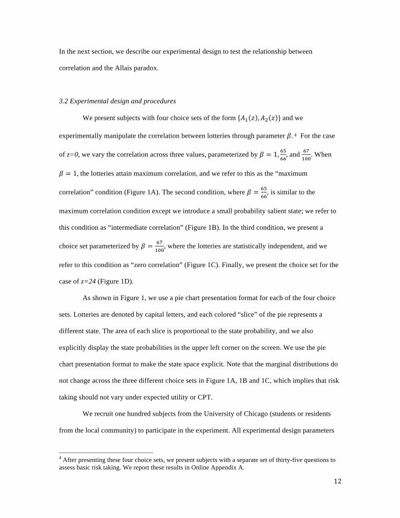
3.2 Experimental design and procedures

We present subjects with four choice sets of the form {𝐴! 𝑧 ,𝐴! 𝑧 } and we

experimentally manipulate the correlation between lotteries through parameter 𝛽. 4 For the case

of z=0, we vary the correlation across three values, parameterized by 𝛽 = 1, !"!!, and

!"!""

. When

𝛽 = 1, the lotteries attain maximum correlation, and we refer to this as the “maximum

correlation” condition (Figure 1A). The second condition, where 𝛽 = !"!!

, is similar to the

maximum correlation condition except we introduce a small probability salient state; we refer to

this condition as “intermediate correlation” (Figure 1B). In the third condition, we present a

choice set parameterized by 𝛽 = !"!""

, where the lotteries are statistically independent, and we

refer to this condition as “zero correlation” (Figure 1C). Finally, we present the choice set for the

case of z=24 (Figure 1D).

As shown in Figure 1, we use a pie chart presentation format for each of the four choice

sets. Lotteries are denoted by capital letters, and each colored “slice” of the pie represents a

different state. The area of each slice is proportional to the state probability, and we also

explicitly display the state probabilities in the upper left corner on the screen. We use the pie

chart presentation format to make the state space explicit. Note that the marginal distributions do

not change across the three different choice sets in Figure 1A, 1B and 1C, which implies that risk

taking should not vary under expected utility or CPT.

We recruit one hundred subjects from the University of Chicago (students or residents

from the local community) to participate in the experiment. All experimental design parameters

4 After presenting these four choice sets, we present subjects with a separate set of thirty-five questions to assess basic risk taking. We report these results in Online Appendix A.

13

and planned analyses are pre-registered on asPredicted.org (see Online Appendix D for pre-

registration documents). Both the order of the choice sets and the color of each state are

randomized across subjects. Subjects are told that one of the trials would be selected at random at

the end of the experiment and they would be paid according to their choice on the selected trial5.

In addition to the payoff from one random trial, subjects also receive a $6 show up fee. Before the

experiment begins, subjects are given instructions and a practice problem to become familiar with

the experimental software (experimental instructions are provided in Online Appendix E.) After

the subjects complete the experiment, but before receiving their payoffs, we collect demographic

information, including gender, education, age, and past courses taken in statistics. Average total

earnings, including the show up fee, were $16.82 (minimum: $6, maximum: $36, standard

deviation: $12.07).

3.3 Experimental Results

We begin by reporting the propensity to choose lottery 𝐴! 0 for each of the different

correlation conditions. For all values of 𝛿 ∈ (0,1), BGS predict that the probability of choosing

𝐴! 0 will decrease in correlation. The data is consistent with this prediction as the proportion of

subjects who choose lottery 𝐴!(0) decreases from 51% to 41% as the lotteries shift from zero

correlation to intermediate correlation, and from 41% to 20% as the correlation shifts from

intermediate to maximum correlation (p < 0.001, F-test under null that proportions are equal).

Using these choice results, we can now compute the proportion of subjects who exhibit

the Allais paradox under each correlation structure, where we define the Allais paradox as

choosing lottery 𝐴! 0 and choosing lottery 𝐴!(24). Figure 2 shows that the propensity to exhibit

5 There was a 23% chance that each of the four choice sets was chosen. The remaining 8% was allocated to a subsequent set of thirty-five problems that we presented to subjects to assess basic risk taking. (Results from the subsequent set of decision problems are summarized in Online Appendix A.) We used this non-uniform distribution of trial selection in order to incentivize all problems, while putting most of the mass on the Allais Paradox questions (Azrieli, Chambers, and Healy 2017). Once the random trial was selected, and if the subject chose a risky lottery on the selected trial, the random outcome of the risky lottery was determined by the subject, who rolled a pair of 10-sided die.

14

the Allais paradox decreases monotonically with correlation. The propensity decreases from 49%

to 36% as the lotteries shift from zero correlation to intermediate correlation (p = 0.047, two-

tailed t-test). As the correlation increases from intermediate to maximum, the propensity declines

further from 36% to 15% (p = 0.001, two-tailed t-test). The data are therefore consistent with

Proposition 2, which states that the Allais paradox decreases in the correlation between lotteries.

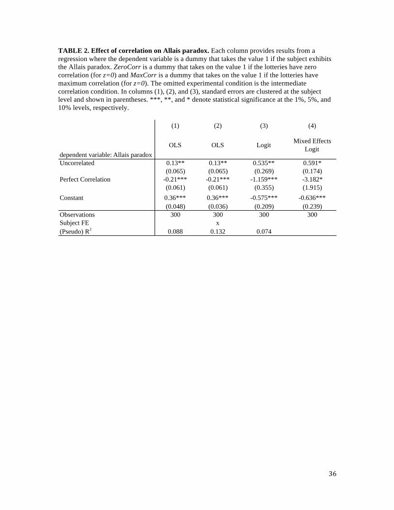
Table 2 displays more detailed tests using a variety of regression models. In the first

column, we run the following OLS regression:

𝑦!,! = 𝛼 + 𝛽!𝑍𝑒𝑟𝑜𝐶𝑜𝑟𝑟! + 𝛽!𝑀𝑎𝑥𝐶𝑜𝑟𝑟! + 𝜀!,! (8)

where each observation is at the subject-trial level, and the dependent variable, 𝑦!,! , takes on the

value 1 if subject i exhibits the Allais paradox on trial t.6 𝑍𝑒𝑟𝑜𝐶𝑜𝑟𝑟 is a dummy that takes on the

value 1 if the trial belongs to the condition where the two lotteries have zero correlation when

z=0; 𝑀𝑎𝑥𝐶𝑜𝑟𝑟 is a dummy that takes on the value 1 if the trial belongs to the condition where the

two lotteries exhibit maximum correlation when z=0. The omitted experimental condition is the

intermediate correlation condition, and the constant therefore provides the propensity to exhibit

the Allais paradox when the lotteries have intermediate correlation. In this regression framework,

for any 𝛿 ∈ 0,1 , salience theory predicts that 𝛽! > 0 and 𝛽! < 0.

The point estimates in column (1) of Table 2 confirm the basic difference in means

results from above, as 𝛽!is significantly positive and 𝛽! is significantly negative. Column (2)

adds a subject fixed effect that controls for heterogeneity across subjects in the overall propensity

to exhibit the Allais paradox. We run a logistic regression in column (3), and a mixed effects

logistic regression in column (4) that includes a random intercept and a random slope on each of

the two dummy variables. We cluster standard errors at the subject level in all specifications

6 Each observation in this regression uses a subject’s decision from two choice sets, one when z=0 and one when z=24, to code the Allais paradox.

15

except for the mixed effects model in (4). Overall, the results from each of the four specifications

supports the BGS prediction that the propensity to exhibit the Allais paradox declines

monotonically in correlation.

Although the data from this experiment consist of only four binary choices per subject, it

is worth emphasizing how starkly different the predictions between salience theory, CPT and

expected utility are for these four questions. Because expected utility and CPT only take as input

the marginal payoff distribution of each lottery, both theories predict that there are no differences

in the propensity to exhibit the Allais paradox as the correlation changes. The data in Figure 2 are

therefore inconsistent with the predictions from all parameterizations of expected utility and CPT.

While these data cannot be explained with expected utility or CPT, an alternative theory

of choice under risk, regret theory, does predict that risk taking will change with the correlation

between lotteries (Starmer 1992; Starmer and Sugden 1993; Leland 1998). Regret theory departs

from expected utility by adding an extra “regret/rejoice” term to the utility function, which

captures the idea that a DM also derives utility from the difference between the outcome he

receives and the outcome he would have received from choosing the alternative lottery. If the

outcome he receives is smaller than what he could have received from choosing the alternative

lottery (in the same state), he experiences regret; otherwise, he experiences rejoice. Our

correlation manipulation directly affects the set of payoff comparisons, and thus regret theory also

predicts that risk taking will vary with correlation. However, it is important to emphasize that

regret theory operates through an additional term in the utility function, whereas salience theory

operates through attention modulated decision weights. The two theories are therefore built on

fundamentally different psychological mechanisms, and in our next experiment, we provide a test

of this mechanism7.

7 In Online Appendix A, we also provide additional behavioral analyses in order to separate regret theory from salience theory. Specifically, we show that individual differences in the sensitivity to correlation in the Allais paradox are themselves correlated with individual differences in risk taking in a separate task.

16

4. EXPERIMENT TWO: MEASURING ATTENTION WITH EYETRACKING DATA

In this experiment, we provide a test of the psychological mechanism proposed in

salience theory. One challenge in testing this mechanism is obtaining measures of attention

during the decision-making process; we address this by collecting eyetracking data while subjects

make a series of lottery choices. The combination of direct measures of attention and data on

lottery choices provides an environment in which we can test the relationship between attention

and risk taking.

4.1 Experimental design

On each of twenty-five trials, a subject is presented with a choice set consisting of a risky

lottery and a certain option. The risky lottery’s payoff distribution is given by,

𝑅 = (𝑔, 0.5; 𝑙, 0.5) while the payoff distribution for the certain option is given by, 𝐶 = 𝑐, 1 ,

where 𝑔 > 𝑐 > 𝑙 ≥ 0. There are thus two equally likely states of the world, 𝑠 ∈ {𝑔𝑎𝑖𝑛, 𝑙𝑜𝑠𝑠}. In

the 𝑔𝑎𝑖𝑛 state, the risky lottery delivers the payoff 𝑔, and in the 𝑙𝑜𝑠𝑠 state, the risky lottery

delivers payoff 𝑙. We vary the certain option payoff, 𝑐, over the set {10, 15, 20, 25, 30} and we

vary the ratio of expected values, ![!]![!]

over the set {1, 1.25, 1.5, 1.75, 2}. We fix “losses,”

𝑐 − 𝑙 = 10, for all trials and the parameters for each trial are shown in Table 3.

A screenshot from an example trial is shown in Figure 3A. We use a similar pie chart

presentation format to the one used in the previous experiment, except the “slices” are separated

along the vertical axis to allow better identification of the state to which a subject is paying

attention. The locations of the gain and loss states are randomized across trials (left or right), and

the locations of the risky lottery and certain option are also randomized across trials (top row or

bottom row). This randomization is important because it controls for any left-right or top-bottom

bias in eye movements that subjects may have if they are accustomed to reading in this direction.

These correlated individual differences are predicted by salience theory, but they are only predicted by regret theory with additional assumptions about the functional form of “choiceless” utility.

17

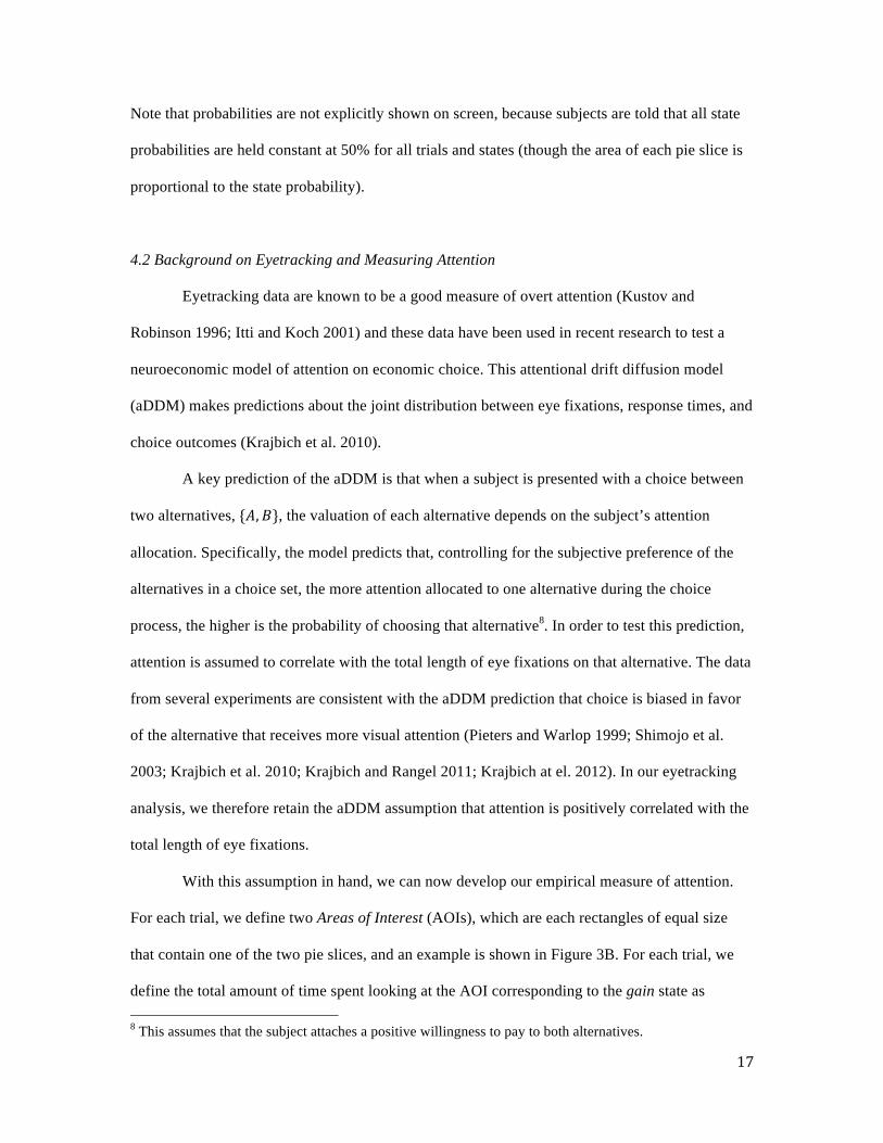
Note that probabilities are not explicitly shown on screen, because subjects are told that all state

probabilities are held constant at 50% for all trials and states (though the area of each pie slice is

proportional to the state probability).

4.2 Background on Eyetracking and Measuring Attention

Eyetracking data are known to be a good measure of overt attention (Kustov and

Robinson 1996; Itti and Koch 2001) and these data have been used in recent research to test a

neuroeconomic model of attention on economic choice. This attentional drift diffusion model

(aDDM) makes predictions about the joint distribution between eye fixations, response times, and

choice outcomes (Krajbich et al. 2010).

A key prediction of the aDDM is that when a subject is presented with a choice between

two alternatives, {𝐴,𝐵}, the valuation of each alternative depends on the subject’s attention

allocation. Specifically, the model predicts that, controlling for the subjective preference of the

alternatives in a choice set, the more attention allocated to one alternative during the choice

process, the higher is the probability of choosing that alternative8. In order to test this prediction,

attention is assumed to correlate with the total length of eye fixations on that alternative. The data

from several experiments are consistent with the aDDM prediction that choice is biased in favor

of the alternative that receives more visual attention (Pieters and Warlop 1999; Shimojo et al.

2003; Krajbich et al. 2010; Krajbich and Rangel 2011; Krajbich at el. 2012). In our eyetracking

analysis, we therefore retain the aDDM assumption that attention is positively correlated with the

total length of eye fixations.

With this assumption in hand, we can now develop our empirical measure of attention.

For each trial, we define two Areas of Interest (AOIs), which are each rectangles of equal size

that contain one of the two pie slices, and an example is shown in Figure 3B. For each trial, we

define the total amount of time spent looking at the AOI corresponding to the gain state as

8 This assumes that the subject attaches a positive willingness to pay to both alternatives.

18

GainTime while the total amount of time spent looking at the AOI corresponding to the loss state

as LossTime. Because we are interested in relative attention, we define our key variable as

𝑅𝑒𝑙𝑎𝑡𝑖𝑣𝑒𝐺𝑎𝑖𝑛𝑇𝑖𝑚𝑒 = 𝐺𝑎𝑖𝑛𝑇𝑖𝑚𝑒−𝐿𝑜𝑠𝑠𝑇𝑖𝑚𝑒

𝐺𝑎𝑖𝑛𝑇𝑖𝑚𝑒+𝐿𝑜𝑠𝑠𝑇𝑖𝑚𝑒. As this variable increases, we interpret this as an increase

in attention to the gain state relative to the loss state. Therefore, under the BGS theory, we expect

that the probability of choosing the risky lottery should increase with 𝑅𝑒𝑙𝑎𝑡𝑖𝑣𝑒𝐺𝑎𝑖𝑛𝑇𝑖𝑚𝑒.

4.3 Experimental procedures

We recruit sixteen undergraduate subjects from the University of Southern California for

the eyetracking experiment9. Each subject enters the lab one at a time, is seated in front of a

computer with eyetracking equipment, and is given instructions about the experimental protocol,

which are provided in Online Appendix E. A nine-point eyetracking calibration procedure is used

to set up the equipment and ensure a precise recording of the eyetracking data. Each subject then

completes three practice trials to familiarize himself with the task.

On each trial, subjects are instructed to decide which of the two alternatives they prefer

by pressing the space bar and verbally indicating their preferred alternative. Before each trial, a

fixation cross is placed for two seconds in the center of the screen and subjects are asked to

maintain fixation on the cross. This ensures that the initial eye fixation does not fall on either of

the two slices, which could potentially bias the total gaze duration.

During the experiment, the eyetracker (Gazepoint GP3) records subjects’ viewing

patterns as they examine the lotteries and make their choices. Specifically, we collect the

location, duration, and pupil diameter of each eye gaze at a rate of sixty times per second10. As in

9 This sample size may appear small relative to a typical economics experiment, but it is standard practice in visual psychophysics. One reason for this is that, while the number of subjects is small, we obtain a large amount of data per subject as we collect data on eye locations sixty times per second per subject. 10 In our analyses, we focus exclusively on fixation duration and fixation location. While pupil dilation is another candidate proxy for salience detection, we do not analyze it here because the pupil dilation latency is too slow to compute state specific measures within a trial. In future work, one could run a modified experimental design where states are separated temporally (rather than across pie slices at the same time), which would enable a test of the relationship between pupil dilation and salience measures.

19

the previous experiment, one trial is drawn at random at the end of the experiment, and subjects

are paid according to their choice on this trial. If the subject chooses the risky lottery, a two-sided

fair coin is used to resolve the risk. Average total earnings, including the show up fee, were

$20.19 (minimum: $5, maximum: $35, standard deviation: $10.42).

4.4 Experimental results

We begin by reporting basic risk taking results for this experiment. The last column of

Table 3 provides the proportion of subjects who choose the risky lottery on each of the twenty-

five trials. Overall, subjects choose the risky lottery on 59% of trials. The data also indicate that,

holding constant the loss and certain amount, there is a substantial increase in risk taking as the

gain amount increases. In other words, as we fix the salience of the loss state, risk taking

increases in the salience of the gain state, which is consistent with salience theory.11

4.4.1 Testing the association between attention and risk taking

We now conduct a test of whether attention allocation biases risky choice in the manner

proposed by salience theory. We test this by assessing whether the relative attention to the gain

state is positively correlated with the probability of choosing the risky lottery. While this

prediction is similar to the prediction from the aDDM discussed above, there is an important

distinction: our test is about the impact of attention on different attributes rather than the impact

of attention on different alternatives.

We proceed by running a logistic regression of the probability of choosing the risky

lottery on RelativeGainTime. Table 4 column (1) shows that there is a significant and positive

correlation between the probability of choosing the risky lottery and the amount of time a subject

11 In contrast to the risk taking results in our first experiment, this pattern of behavior is also consistent with expected utility and CPT. This is due to the fact that, all else equal, as the value of the gain amount increases, the utility of the risky lottery increases relative to the certain option. This prediction also holds under salience theory, but it is amplified by the fact that the decision weight attached to the gain state endogenously increases in the gain amount, due to the ordering property of the salience function.

20

spends looking at the gain state relative to the loss state. Column (2) adds subject fixed effects

and we see that the coefficient on RelativeGainTime remains significantly positive. This indicates

that for a given subject, fluctuations in attention across the twenty-five choice sets have a

systematic impact on risk taking.

We can also investigate the effect of attention on risk taking across subjects. As

mentioned above, the average subject chooses the risky lottery on 59% of trials. However, there is

a substantial amount of heterogeneity in risk-taking across subjects: the minimum propensity of

choosing the risky lottery is 36% and the maximum is 80%. We test whether individual

differences in attention can explain this heterogeneity by re-estimating the model in column (1)

and adding choice set fixed effects. Therefore, the marginal effect of RelativeGainTime on risk

taking is identified off of variation across subjects. Column (3) shows that the coefficient on

RelativeGainTime is significantly positive. Thus, for a given choice set, those subjects who

allocate more attention to the risky lottery’s upside exhibit a higher probability of choosing the

risky lottery. This result suggests that, while individual variation in risk taking is often attributed

to differences in stable risk aversion coefficients, attention may also be a fundamental source of

heterogeneity in risk-taking.

4.4.2 Testing the association between payoffs and attention allocation

The results in the previous section document a correlation between attention and risk

taking, but they raise an important question: what governs attention allocation? Salience theory

proposes that attention is allocated according to a salience function that satisfies the two

properties of ordering and diminishing sensitivity. While our experiment is not optimized to

provide a general test of these two properties, we use the eyetracking data to test one specific

salience function.

We conduct this test by assessing whether 𝑅𝑒𝑙𝑎𝑡𝑖𝑣𝑒𝐺𝑎𝑖𝑛𝑇𝑖𝑚𝑒, our empirical measure of

relative attention to the gain state, is greater for trials when the gain state is salient compared to

21

when the loss state is salient. The first step in the analysis is to compute the salience of each state,

which entails making a non-trivial assumption about the functional form of salience. We assume

the specific salience function defined in equation (2), which contains the diminishing sensitivity

parameter, 𝜃. In order to estimate 𝜃, we conduct a maximum likelihood estimation of the salience

model using the choice data, and we jointly estimate the salience parameter 𝛿. We pool all

subjects and estimate the model parameters 𝜃 and 𝛿 at the group level, and find that the best

fitting parameter estimates are 𝛿 = 0.21 and 𝜃 = 0.05 (further details on the estimation

procedure are provided in the Appendix).

We can now compute the salience of each state, conditional on the best fitting

diminishing sensitivity parameter estimate, 𝜃 = 0.05. The difference in salience between the

gain and loss states is summarized by the variable, 𝑆𝑎𝑙𝑖𝑒𝑛𝑐𝑒𝐷𝑖𝑓𝑓 = 𝜎 𝑔, 𝑐 − 𝜎 𝑙, 𝑐 . When this

variable is positive, the gain state is salient (56% of trials), and when the variable is negative, the

loss state is salient (44% of trials). Column (1) of Table 5 shows results from a regression of

RelativeGainTime on GainSal, which is a dummy that takes the value 1 if the gain state is salient,

and 0 otherwise. The coefficient on GainSal is not significantly different from zero, indicating

that there is no difference in mean attention allocation on trials where the gain state is salient

compared to trials where the loss state is salient. Column (2) tests for a linear effect of attention

allocation on the difference in model based salience across states, 𝑆𝑎𝑙𝑖𝑒𝑛𝑐𝑒𝐷𝑖𝑓𝑓, but we find the

coefficient is not significantly different from zero.

One concern with the results in column (1) is that, for some trials, the classification of

whether the gain state is salient depends on parameter 𝜃 in the salience function. Because we

structurally estimate this parameter using choice data, the resulting parameter estimate, 𝜃 =

0.05, is potentially subject to misspecification in other parts of the salience model (e.g., the value

function). We therefore re-estimate this regression, restricting to the subset of trials (76%) for

22

which the salience classification is independent of parameter 𝜃. After repeating our tests on this

restricted sample (columns (3) and (4)), we find that our results do not change.

The results in Table 5 are therefore inconsistent with the specific salience function

defined in (2). However, it is important to emphasize that our eyetracking data do not allow for a

general test of the ordering and diminishing sensitivity properties that characterize the class of

salience functions proposed by BGS12. Moreover, because the risk-taking predictions from our

first experiment hold for all salience functions (Proposition 2), it is certainly plausible that the

Allais results we observe in that experiment are generated through a different salience function

than the one we test here.

Another important possibility is that attention allocation may be governed by stable risk

preferences. While our eyetracking data provide strong evidence of a correlation between

attention and risky choice, we cannot say anything about the direction of causality. It is therefore

possible that the correlation we document is the result of risk preferences causally affecting

attention allocation. In the next section, we conduct our third and final experiment to establish the

direction of causality.

5. EXPERIMENT THREE: TESTING FOR CAUSALITY

BETWEEN ATTENTION AND VALUATION

The link between attention and valuation can run in both directions. Salience theory

emphasizes the role that ex-post attention plays in shaping risk attitudes, and thus the theory

proposes that attention affects the valuation of risky lotteries. The opposite direction of causality

can also hold: the valuation of lotteries or states can affect attention allocation. This latter

direction of causality is consistent with theories of rational inattention (Sims 2003; Woodford

2009; Caplin and Dean 2015). In order to test for an ex-post allocation of attention, we design an

12InOnline Appendix B we provide a post-hoc test of the ordering property that provides evidence qualitatively consistent with the ordering property.

23

experiment where we exogenously vary attention through a “visual salience” manipulation of the

choice set. We vary the visual layout of the payoffs while holding constant the magnitude of

payoffs, and then test for an impact on risky choice.

5.1 Experimental design

We collect data from an additional three hundred subjects on Amazon Mechanical Turk

(mTurk), which is an online data collection platform. One advantage of mTurk over a laboratory

environment is the ability to collect data from a larger and more diverse pool of subjects; the

disadvantage is that the remote nature of the data collection reduces experimental control. The

mTurk platform has become increasingly popular in economic research (Olea and Strzalecki

2014; Ambuehl, Niederle, and Roth 2015; Lian, Ma, Wang 2016), and there is evidence that it

provides response quality that is similar to that in lab experiments (Casler, Bickel, and Hackett

2013).13

The subjects we recruit from mTurk make decisions over thirty-five trials, where each

trial consists of a risky lottery and a mean preserving certain option. We define the risky lottery

by 𝑅 = (𝑔, 𝑝; 𝑙, 1 − 𝑝) while the payoff distribution for the certain option is given by, 𝐶 =

𝑐, 1 and 𝑔 > 𝑐 > 𝑙 ≥ 0. As in the previous experiment, there are two states of the world,

𝑠 ∈ {𝑔𝑎𝑖𝑛, 𝑙𝑜𝑠𝑠}. In the 𝑔𝑎𝑖𝑛 state, the risky lottery delivers payoff 𝑔, which is a gain relative to

the certain option; in the 𝑙𝑜𝑠𝑠 state, the risky lottery delivers payoff 𝑙, which is a loss relative to

the certain option. We fix “losses,” 𝑐 − 𝑙 = 20, for all trials. The parameter values for all trials

13 The mTurk platform consists of “requesters” who hire “workers” to complete jobs in exchange for monetary compensation. After a worker completes a job, the requester decides based on the quality of the job whether to approve the job for compensation. Before hiring a worker, a requester can filter potential workers based on the worker’s historical approval rate. In order to ensure high quality data collection, we restrict participation to individuals who have an approval rate of 95% or higher and who reside in the US.

24

are given in Table 6. In contrast to the incentive structure in Experiment 2, our subjects from

mTurk make hypothetical choices and are paid $1.50 for completing the task14.

We employ a within subjects design with three conditions, as shown in Figure 4. In the

control condition, choice sets are presented as pie charts, where the area of each slice of the pie is

proportional to its state probability. We also explicitly display the probability of each state in the

upper left hand corner on each trial. In the Gain treatment, we increase the visual salience of the

gain state by making both the background color and font of the loss state more faint. Specifically,

we increase the transparency of the color and font of the loss state to 60%, which makes the gain

state “pop out” (since we keep the transparency of the gain state at 0%). Conversely, in the Loss

treatment, we increase the transparency of the gain state to 60%, which makes the loss state “pop

out” (since we keep the transparency of the loss state at 0%). This method of visual salience

manipulation is similar to that used in Milosavljevic et al. (2012), and we randomize these three

conditions at the trial-subject level. In this experiment, we have two sources of salience. To

clearly distinguish between the two sources, we refer to the first source of salience proposed in

BGS as “economic salience.” We refer to the second source of salience, generated through the

visual transparency manipulation, as “visual salience.”

If attention allocation causally affects valuation and choice, then we expect our visual

salience manipulation to systematically shift average levels of risk taking. In particular, we expect

that in the Loss treatment, subjects to overweigh the payoffs in the loss state and therefore choose

the risky lottery less often than in the control condition. In the Gain treatment, we expect subjects

to overweigh payoffs in the gain state and therefore choose the risky lottery more often than in

the control condition.

Our experiment was pre-registered on Aspredicted.org, and contains details on the

14 Because subjects in this experiment make decisions over the same set of thirty-five that subjects in the laboratory make at the end of Experiment 1, we are able to formally test whether risk-taking is systematically different on mTurk compared to risk-taking in the lab where there are strong monetary incentives. In Online Appendix C, we show that risk taking is very similar across the two samples, suggesting that the difference in incentives does not have a major impact on behavior in the current task.

25

sample size, number of conditions, and predictions to be tested. The details of the pre-registration

are given in Online Appendix D. The average age of subjects in this sample was 37.4 (standard

deviation: 11.0), 57% were male, 73% had college degrees and a vast majority (86%) had not

taken a statistics class in the past five years.

5.2 Experimental results

We first examine whether risk taking in the control condition is consistent with the

predictions of the BGS theory. For each trial, we compute whether the gain state is economically

salient using the same definition as in previous experiment (the salience function in (2) and

setting 𝜃 = 0.05). The probability of choosing the risky lottery increases from 30.5% when the

loss state is economically salient to 47.9% when the gain state is economically salient (p < 0.001,

two sided t-test) 15. There are similar effects in the treatment conditions; in the Gain treatment, the

probability of choosing the risky lottery increases from 30.7% when the loss state is economically

salient to 46.2% when the gain state is economically salient (p < 0.001, two sided t-test). In the

Loss treatment, the probability of choosing the lottery increases from 28.5% when the loss state is

economically salient to 45.3% when the gain state is economically salient (p < 0.001, two sided t-

test). In sum, basic variation in risk taking within each experimental condition is consistent with

salience theory.

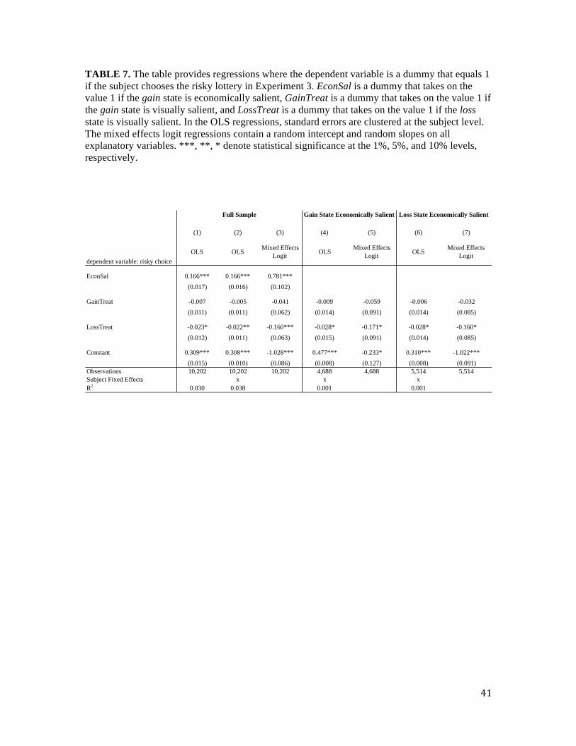
Table 7 reports results of the tests for treatment effects. In Column (1) we run an OLS

regression where the dependent variable is a dummy that takes the value 1 if the subject chooses

the risky lottery; EconSal is a dummy equal to 1 if the gain state is economically salient,

GainTreat is a dummy that takes on the value 1 if the trial is in the Gain treatment, and LossTreat

is a dummy that takes on the value 1 if the trial is in the Loss treatment. The intercept therefore

15 We excluded 7 of the 300 subjects because they completed the entire task in a very short amount of time (under 200 seconds) and were unlikely paying sufficient attention to the task. Additionally, due to a software glitch we lost one trial for fifty-three of our subject (trial 3 in Table 6), and so these trials are not included in any subsequent analyses.

26

provides the average level of risk taking in the control condition for trials where the loss state is

economically salient.

The results in columns (1) – (3) indicate that the coefficient on the LossTreat variable is

significantly negative in each specification. Columns (1) and (2) provide results from an OLS

model, and we find that the average level of risk taking is reduced by 2.2% when the loss state is

made visually salient. This result is robust to a mixed effects logistic specification, which allows

for heterogeneity across subjects in the response to manipulating the visual salience of the loss

state. In columns (4) – (7) we provide subsample analysis where we split the data into those trials

where the gain state is economically salient and those trials where the loss state is economically

salient. The strength of the effect becomes smaller, but the results remain significant at the 10%

level in all four specifications. It is also worth noting that the relative strength of the visual

salience effect is much smaller than the strength of the economic salience effect. For example, the

coefficient on the EconSal variable in column (2) indicates that the marginal effect of making the

gain state economically salient is a 16.6% increase in risk taking. The marginal effect of making

the loss state visually salient is approximately one-sixth of this size.

While we find a significant effect in the Loss treatment, we do not find a similar

treatment effect when increasing the visual salience of the gain state. In all seven specifications of

Table 7, the coefficient on the GainTreat variable is not statistically different from zero. Our data

therefore indicate that there is an asymmetric impact of visual salience on risk taking. One

potential post-hoc explanation for this asymmetry is that the visual salience manipulation is

stronger for the Loss treatment compared to the Gain treatment. In particular, the average

probability of the gain state in our experiment is much smaller than the average probability of the

loss state (the gain state is typically characterized by a low probability and high payoff). Because

our manipulation operates through making a visual representation of the state more salient –

where the size of the visual representation is proportional to the state probability – the visual

salience treatment may have had a larger effect in the Loss treatment compared to the Gain

27

treatment. This could make it harder to detect a treatment effect in the Gain treatment compared

to the Loss treatment. Another possibility is that losses may be more economically salient than

gains. Under this scenario, an exogenous increase in attention to the loss state may exert a larger

effect on risk preferences compared to the same increase in attention to the gain state. However,

we emphasize that both of these explanations are clearly post-hoc and more data is needed to test

each of them.

Finally, even though our experimental design enables us to test for the causal effect of

attention on valuation, we cannot use our data to test for a causal effect of valuation on attention

allocation. This channel is also potentially active in our experiment, and moreover, if causality

does run in both directions, it becomes important in future work to understand the dynamics of

the feedback loop between attention and valuation (Shimojo et al. 2003; Gottlieb 2012).

6. DISCUSSION

In this paper, we conduct three experiments that combine eyetracking data with careful

experimental design to test salience theory. In the first experiment, we manipulate the joint

distribution between two Allais style lotteries, while holding the marginal distribution of each

lottery constant. The manipulation has a systematic impact on risk taking in the direction

predicted by salience theory, and at the same time, the results are inconsistent with all

parameterizations of expected utility and CPT. The eyetracking data provide evidence that

attention to the risky lottery’s upside, relative to its downside, is correlated with the probability of

choosing the risky lottery. This result holds for a given choice set, which demonstrates that

individual differences in attention can explain variation in risk taking across subjects. Finally, we

show that increasing the visual salience of the risky lottery’s downside causally decreases risk

taking, but we do not find a symmetric effect when increasing the visual salience of the risky

lottery’s upside. No single piece of our experimental evidence is decisive, but when taken

28

together, salience theory provides a parsimonious explanation for the broad set of experimental

results.

While each of our three experiments is useful in testing a different aspect of the

relationship between payoffs, attention, and risk preferences, one may wonder whether it is

feasible to perform all of our tests using a single experiment. For example, an alternative design

could combine our first experiment, which varies the correlation between lotteries, with a visual

salience treatment and simultaneously record eyetracking data. This design would provide the

advantage that all measurements are obtained within the same experiment, but there at least two

concerns with this approach. First, the complexity of the state space would hamper our ability to

conduct the basic eyetracking tests. Because there are four states in the Allais choice sets, each

with a different probability, we would need to impose extra structure on our empirical tests to

control for these probabilities. In our eyetracking experiment, we are able to sidestep this

difficulty by setting all state probabilities to 0.516. Second, eyetracking data are noisy, and thus

we require more than four trials to generate sufficient statistical power to test for attention effects.

Statistical power is also a concern for the visual salience experiment, where effect sizes are

typically small,17 which is why we collect data from many subjects and trials. However, we

believe these concerns are only temporary as future work in neuroeconomics is likely to provide

the additional structure needed to conduct eyetracking tests in more general environments.18

While we find a strong correlation between attention and risk taking in our second

experiment, a limitation of our design is that we cannot use the eyetracking data to test the

general properties that characterize the salience function proposed by BGS. The eyetracking

16 In general, because attention is likely to be modulated by payoffs and probabilities, extra structure is needed to test how the interaction between probabilities and payoffs affects attention allocation. If instead, all probabilities are held constant at 0.5, as we impose in our design, then we can perform our experimental tests without relying on additional assumptions. 17 Previous work shows that effect sizes for visual salience on choice are small relative to effects of subjective value (Milosavljevic et al. 2012). This is consistent with our results where we find that the effect size of the Loss treatment is approximately one-sixth of the economic salience effect size. 18 Krajbich and Rangel (2011) have already begun to extend the aDDM to environments with more than two alternatives.

29

results we report are inconsistent with the specific salience function defined in equation (2), but

we cannot rule out that the data are generated by a different salience function. Moreover, because

our risk taking results from the first experiment are predicted by all salience functions, those data

may also have been generated by a different salience function. Therefore, an important direction

for future research is to design an experiment that is optimized to test the general properties of

ordering and diminishing sensitivity. Future work can also build on the eyetracking methods

presented here to estimate the salience function over a wide domain of payoffs. Estimating the

salience function exclusively from attention data has the advantage that no assumptions are

needed on how salience affects valuation (e.g., there is no need to estimate 𝛿 or make

assumptions about the value function). One could then directly test whether the estimated salience

function exhibits the properties that characterize the general class of salience functions.

We conclude with one additional direction for future research. In their original paper,

BGS suggest that when the correlation structure between lotteries is unspecified, a decision maker

perceives the lotteries within a choice set to be uncorrelated. Such an assumption can explain the

robustness of the Allais paradox when the correlation structure is not specified, since salience

theory predicts the Allais paradox will arise when the two lotteries are uncorrelated. Our data

provide some extra support for this assumption and offer a potential reason why a DM’s default

perception is that lotteries are uncorrelated. There are an infinite number of correlation structures

(parameterized by 𝛽 in Table 1), but of course, only one correlation structure where the two

lotteries are statistically independent. This leads us to conjecture that when the state space is not

explicitly defined, a decision-maker defaults to perceiving the unique correlation structure

characterized by statistical independence. This is certainly not the only mechanism by which an

unspecified correlation structure can impact risk-taking. It is likely that the perception of the state

space – and more generally the “consideration set” – is governed by those attributes and states of

a decision problem that receive the most attention (Caplin, Dean, and Leahy 2016). Given the

30

importance that the state space has in explaining risk-taking over binary lottery choice, we

believe that understanding the perception of correlation is an important step for future research.

31

REFERENCES

Agranov, Marina and Pietro Ortoleva, “Stochastic Choice and Preferences for Randomization,” Journal of Political Economy, 125 (2017), 40-68.

Allais, Maurice, “Le Comportement de l’Homme Rationnel devant le Risque: Critique des Postulats et Axiomes de l’Ecole Americaine,” Econometrica, 21 (1953), 503-546.

Ambuehl, Sandro, Muriel Niederle, and Alvin Roth, “More Money, More Problems? Can High Pay Be Coercive and Repugnant?” American Economic Review 105, (2015), 357-360.

Azrieli, Yaron, Christopher Chambers, and Paul J Healy, “Incentives in Experiments: A Theoretical Analysis” Journal of Political Economy (2017), forthcoming.

Bell, David, “Regret in Decision Making Under Uncertainty,” Operations Research 30 (1982), 961-981.

Bordalo, Pedro, Nicola Gennaioli, and Andrei Shleifer, “Salience Theory of Choice Under Risk,” Quarterly Journal of Economics 127 (2012), 1243-1285.

Bordalo, Pedro, Nicola Gennaioli, and Andrei Shleifer, “Salience and Consumer Choice,” Journal of Political Economy 121 (2013), 803-843.

Bushong, Benjamin, Matthew Rabin, and Joshua Schwartzstein, “A Model of Relative Thinking,” (2016), Working paper.

Caplin, Andrew and Mark Dean, “Revealed Preference, Rational Inattention, and Costly Information Acquisition,” American Economic Review, 105 (2015), 2183-2203.

Caplin, Andrew, Mark Dean, and John Leahy, “Rational Inattention, Optimal Consideration Sets and Stochastic Choice,” (2016), Working paper.

Casler, Krista, Lydia Bickel and Elizabeth Hackett, “Separate but Equal? A Comparison of Participants and Data Gathered via Amazon’s MTurk, Social Media, and Face-to-Face Behavioral Testing,” Computers in Human Behavior, 29 (2013), 2156-2160.

Cunningham, Tom, “Comparisons and Choice,” (2013), Working paper.

Dertwinkel-Kalt, Markus, Katrin Kohler, Mirjam R.J. Lange and Tobias Wenzel, “Demand Shifts Due to Salience: Experimental Evidence,” Journal of the European Economic Assocation (2016), forthcoming.

Fehr, Ernst, and Antonio Rangel, “Neuroeconomic Foundations of Economic Choice – Recent Advances,” Journal of Economic Perspectives, 25 (2011), 3-30.

Frydman, Cary, and Gideon Nave, “Extrapolative Beliefs in Perceptual and Economic Decisions: Evidence of a Common Mechanism,” Management Science (2016), forthcoming.

32

Fudenberg, Drew, Ryota Iijima, and Tomasz Strzalecki, “Stochastic Choice and Revealed Perturbed Utility,” Econometrica 83 (2015), 2371-2409.

Gabaix, Xavier, “A Sparsity-Based Model of Bounded Rationality,” Quarterly Journal of Economics 129 (2014), 1661-1710.

Gottlieb, Jacqueline, “Attention, Learning, and the Value of Information,” Neuron 76, (2012), 281-295.

Itti, Laurent and Christof Koch, “Computational Modelling of Visual Attention,” Nature Reviews Neuroscience 2, (2001), 194-203.

Khaw, Mel Win, Ziang Li, and Michael Woodford, “Risk Aversion as a Perceptual Bias,” (2017), Working Paper.

Koszegi, Botond and Adam Szeidel, “A Model of Focusing in Economic Choice,” Quarterly Journal of Economics 128 (2013), 53-104.

Krajbich, Ian, Carrie Armel, and Antonio Rangel, “Visual fixations and the computation and comparison of value in simple choice,” Nature Neuroscience 13 (2010), 1292-1298.

Krajbich, Ian and Antonio Rangel, “Multialternative Drift-Diffusion Model Predicts the Relationship Between Visual Fixations and Choice in Value-Based Decisions,” Proceedings of National Academy of Sciences 108, (2011), 13852-13857.

Krajbich, Ian, Dingchao Lu, Colin Camerer and Antonio Rangel, “The Attentional Drift-Diffusion Model Extends to Simple Purchasing Decisions,” Frontiers in Psychology 3, (2012), 1-18.

Kustov, Alexander and David Lee Robinson, “Shared Neural Control of Attentional Shifts and Eye Movements,” Nature 384, (1996), 74-77.

Leland, Jonathan, “Generalized Similarity Judgments: An Alternative Explanation for Choice Anomalies,” Journal of Risk and Uncertainty, 9 (1994), 151-172.

Leland, Jonathan, “Similarity Judgments in Choice Under Uncertainty: A Reinterpretation of the Predictions of Regret Theory,” Management Science, 44 (1998), 659-672.

Lian, Chen, Yueran Ma, and Carmen Wang, “Low Interest Rates and Risk Taking: Evidence from Individual Investment Decisions,” (2016), Working paper.

Loomes, Graham, and Robert Sugden, “Regret Theory: An Alternative Theory of Rational Choice under Uncertainty,” Economic Journal, 92 (1982), 805-824.

Milosavljevic, Milica, Jonathan Malmaud, Alexander Huth, Christof Koch, and Antonio Rangel, “The Drift Diffusion Model Can Account for the Accuracy and Reaction Time of Value-Based Choices Under High and Low Time Pressure,” Judgment and Decision Making, 5 (2010), 437-449.

33

Milosavljevic, Milica, Vidhya Navalpakkam, Christof Koch, and Antonio Rangel, “Relative Visual Saliency Differences Induce Sizable Bias in Consumer Choice,” Journal of Consumer Psychology, 22 (2012), 67-74.

Olea, Jose Luis Montiel and Tomasz Strzaelcki, “Axiomatization and Measurement of Quasi-Hyperbolic Discounting,” Quarterly Journal of Economics, 129 (2014), 1449-1499.

Pieters, Rik and Luk Warlop, “Visual Attention During Brand Choice: The Impact of Time Pressure and Task Motivation,” International Journal of Research in Marketing, 16 (1999), 1-16.

Ratcliff, Roger, “A Theory of Memory Retrieval,” Psychological Review, 85 (1978), 59-108.

Rubinstein, Ariel, “Similairty and Decsion-Making Under Risk (Is there a Utiltiy Theory Resolution to the Allais Paradox?” Jounal of Economic Theory, 46 (1988), 145-153.

Schwartzstein, Joshua, “Selective Attention and Learning,” Journal of the European Economic Association, 12 (2014), 1423-1452.

Shimojo, Shinsuke, Claudiu Simion, Eiko Shimojo, and Christian Scheier, “Gaze Bias Both Reflects and Influences Preference,” Nature Neuroscience, 6 (2003), 1317-1322.

Sims, Christopher, “Implications of Rational Inattention,” Journal of Monetary Economics, 50 (2003), 665-690.

Starmer, Chris, “Testing New Theories of Choice Under Uncertainty Using the Common Consequence Effect,” Review of Economic Studies, 59 (1992), 813-830.

Starmer, Chris, and Robert Sugden, “Testing for Juxtaposition and Event-Splitting Effects,” Journal of Risk and Uncertainty, 6 (1993), 235-254.

Summerfield, Christopher, and Konstantinos Tsetsos, “Building Bridges Between Perceptual and Economic Decision-Making: Neural and Computational Mechamisms,” Frontiers in Neuroscience, 6 (2012), 1-20.

Towal, Blythe, Milica Mormann, and Christof Koch, “Simultaneous Modeling of Visual Saliency and Value Computation Improves Predictions of Economic Choice,” Proceedings of the National Academy of Sciences, 110 (2013), E3858-E3867.

Tversky, Amos and Daniel Kahneman, “Advances in Prospect Theory: Cumulative Representation of Uncertainty,” Journal of Risk and Uncertainty, 5 (1992), 297-323.

Webb, Ryan, “The Dynamics of Stochastic Choice,” (2015), Working Paper.

Wilcox, Nathaniel, “Stochastic Models for Binary Discrete Choice Under Risk: A Critical Primer and Econometric Comparison,” in J.C. Cox and G.W. Harrison, eds., Research in Experimental Economics Vol.12: Risk Aversion in Experiments, 2008, 197-292. Bingley, UK: Emerald.

34

Woodford, Michael, “Information-Constrained State-Dependent Pricing,” Journal of Monetary Economics, 56 (2009), 100-124.

Woodford, Michael, “Optimal Evidence Accumulation and Stochastic Choice,” (2016), Working Paper.

35

TABLE 1. Joint distribution of lotteries 𝐴!(𝑧) and 𝐴! 𝑧 . The columns represent the four states

whereas the rows represent the two lotteries. State probabilities are a function of 𝛽 ∈ !!, 1 ,

which parameterizes the joint distribution. The marginal distributions of 𝐴!(𝑧) and 𝐴! 𝑧 are independent of 𝛽.

!! !! !! !!

Probability 0.66! 0.66(1− !) 0.67− 0.66! 0.33(2! − 1)

!!(!) $z $25 $0 $25

!!(!) $z $0 $24 $24

36

TABLE 2. Effect of correlation on Allais paradox. Each column provides results from a regression where the dependent variable is a dummy that takes the value 1 if the subject exhibits the Allais paradox. ZeroCorr is a dummy that takes on the value 1 if the lotteries have zero correlation (for z=0) and MaxCorr is a dummy that takes on the value 1 if the lotteries have maximum correlation (for z=0). The omitted experimental condition is the intermediate correlation condition. In columns (1), (2), and (3), standard errors are clustered at the subject level and shown in parentheses. ***, **, and * denote statistical significance at the 1%, 5%, and 10% levels, respectively.

(1) (2) (3) (4)

dependent variable: Allais paradox

OLS OLS LogitMixed Effects

Logit

Uncorrelated 0.13** 0.13** 0.535** 0.591*(0.065) (0.065) (0.269) (0.174)

Perfect Correlation -0.21*** -0.21*** -1.159*** -3.182*(0.061) (0.061) (0.355) (1.915)

Constant 0.36*** 0.36*** -0.575*** -0.636***(0.048) (0.036) (0.209) (0.239)

Observations 300 300 300 300Subject FE x(Pseudo) R2 0.088 0.132 0.074

37

TABLE 3. Lottery Payoffs and Choice Data for Experiment 2. The table displays the parameter values used for the twenty-five choice sets in Experiment 2. The risky lottery delivers payoffs g or l, each with 50% probability. The certain option delivers payoff c with 100% probability. The last column provides the percentage of subjects who choose the risky lottery in each trial.

Trial # g l c % choosing Risky Lottery

1 100 20 30 100%2 85 20 30 94%3 70 20 30 88%4 55 20 30 56%5 40 20 30 19%6 85 15 25 94%7 73 15 25 88%8 60 15 25 69%9 48 15 25 75%10 35 15 25 31%11 70 10 20 88%12 60 10 20 88%13 50 10 20 88%14 40 10 20 50%15 30 10 20 31%16 55 5 15 69%17 48 5 15 88%18 40 5 15 38%19 33 5 15 56%20 25 5 15 6%21 40 0 10 50%22 35 0 10 44%23 30 0 10 38%24 25 0 10 13%25 20 0 10 6%

38

TABLE 4. Regression of Choice on Attention. The table provides logistic regression results where the dependent variable takes the value 1 if the subject chooses the risky lottery in that trial. RelativeGainTime is our eyetracking measure of relative attention to the gain state. Standard errors are clustered at the subject level. ***, **, * denote statistical significance at the 1%, 5%, and 10% levels, respectively.

dependent variable: risky (1) (2) (3)

RelativeGainTime 0.444** 0.471* 0.468*(0.217) (0.257) (0.278)

Constant 0.309** 0.690*** -2.830***(0.151) (0.033) (1.084)

Observations 400 400 384Choice Set FE xSubject FE xPseudo R2 0.005 0.060 0.280

39

TABLE 5. Regression of Attention on Payoff Layout. The table provides OLS regression results where the dependent variable is RelativeGainTime, which measures relative attention to the gain state. GainSal is a dummy that takes the value if the gain state is salient, and SalienceDiff is the difference in salience measures between the gain and loss states under the salience function in equation (2). Columns (3) and (4) are restricted to the subsample where the classification of which state is salient is independent of the diminishing sensitivity parameter 𝜃. Standard errors are clustered at the subject level. ***, **, * denote statistical significance at the 1%, 5%, and 10% levels, respectively.

dependent variable: RelativeGainTime (1) (2) (3) (4)

GainSal 0.008 0.029(0.027) (0.032)

SalienceDiff -0.065 -0.030(0.063) (0.073)

Constant 0.079*** 0.080*** 0.057** 0.080***(0.020) (0.010) (0.022) (0.008)

Observations 400 400 304 304R2 0.001 0.003 0.001 0.001

Full Sample Restricted Subset

40

TABLE 6. Experimental Design for Experiment 3. The table displays the parameter values used for the thirty-five choice sets in Experiment 3. The risky lottery delivers payoffs g with probability p, and l with probability 1-p. The certain option delivers payoff c with 100% probability.

Trial Number g l c p1 2000 0 20 0.012 400 0 20 0.053 100 0 20 0.24 61 0 20 0.335 50 0 20 0.46 40 0 20 0.57 30 0 20 0.678 2010 10 30 0.019 410 10 30 0.0510 110 10 30 0.211 71 10 30 0.3312 60 10 30 0.413 50 10 30 0.514 40 10 30 0.6715 2020 20 40 0.0116 420 20 40 0.0517 120 20 40 0.218 81 20 40 0.3319 70 20 40 0.420 60 20 40 0.521 50 20 40 0.6722 2030 30 50 0.0123 430 30 50 0.0524 130 30 50 0.225 91 30 50 0.3326 80 30 50 0.427 70 30 50 0.528 60 30 50 0.6729 2040 40 60 0.0130 440 40 60 0.0531 140 40 60 0.232 101 40 60 0.3333 90 40 60 0.434 80 40 60 0.535 70 40 60 0.67

41

TABLE 7. The table provides regressions where the dependent variable is a dummy that equals 1 if the subject chooses the risky lottery in Experiment 3. EconSal is a dummy that takes on the value 1 if the gain state is economically salient, GainTreat is a dummy that takes on the value 1 if the gain state is visually salient, and LossTreat is a dummy that takes on the value 1 if the loss state is visually salient. In the OLS regressions, standard errors are clustered at the subject level. The mixed effects logit regressions contain a random intercept and random slopes on all explanatory variables. ***, **, * denote statistical significance at the 1%, 5%, and 10% levels, respectively.

(1) (2) (3) (4) (5) (6) (7)

dependent variable: risky choice

OLS OLSMixed Effects

LogitOLS

Mixed Effects Logit

OLSMixed Effects

Logit

EconSal 0.166*** 0.166*** 0.781***

(0.017) (0.016) (0.102)

GainTreat -0.007 -0.005 -0.041 -0.009 -0.059 -0.006 -0.032

(0.011) (0.011) (0.062) (0.014) (0.091) (0.014) (0.085)

LossTreat -0.023* -0.022** -0.160*** -0.028* -0.171* -0.028* -0.160*

(0.012) (0.011) (0.063) (0.015) (0.091) (0.014) (0.085)

Constant 0.309*** 0.308*** -1.028*** 0.477*** -0.233* 0.310*** -1.022***

(0.015) (0.010) (0.086) (0.008) (0.127) (0.008) (0.091)Observations 10,202 10,202 10,202 4,688 4,688 5,514 5,514Subject Fixed Effects x x xR2 0.030 0.038 0.001 0.001

Full Sample Gain State Economically Salient Loss State Economically Salient

42

FIGURE 1. Choice Sets from Experiment 1. Each of the four choice sets is presented to subjects in pie chart form. For each pie chart, the colors denote the different states and letters denote the different lotteries. The size of each “slice” of the pie chart corresponds to the probability of the state, which is summarized on the top left corner of each screen. Panel A: the choice set when z=0 and lotteries have maximum correlation. Panel B: the choice set when z=0 and lotteries have intermediate correlation. Panel C: the choice set when z=0 and lotteries are have zero correlation. Panel D: the choice set when z=24. Colors are randomized at the subject-trial level.

PANEL C: Zero Correlation, z = 0

PANEL B: Intermediate Correlation, z = 0

PANEL A: Maximum Correlation, z = 0

PANEL D: z = 24

43

FIGURE 2: Allais Paradox Decreases with Correlation. Figure displays the proportion of subjects from Experiment 1 who exhibit the Allais paradox for each of the three different correlation structures.

0%

10%

20%

30%

40%

50%

60%

Uncorrelated ImperfectlyCorrelated PerfectlyCorrelated

Percetna

geofS

ubjectsE

xhibi5ng

AllaisParad

ox

p=0.047

p=0.001

ZeroCorrela)on

IntermediateCorrela)on

MaximumCorrela)on

44

FIGURE 3: Screenshot from Eyetracking Experiment and Area Of Interest Analysis. PANEL A shows an example trial where the risky lottery delivers $55 or $5, each with 50% probability. The certain option delivers $15 with certainty. The “slices’ of the pie chart denote states, and the area of each slice is proportional to its state probability. PANEL B shows the rectangles used for the AOI anlaysis, and subjects did not see these rectangles on screen.

PANEL A

PANEL B

45

FIGURE 4: Example Trials from Experiment 3. The figure displays the choice set in each of the three experimental conditions in Experiment 3. PANEL A shows the choice set in the control condition. PANEL B shows the choice in the Gain treatment, where the visual transparency of the loss state is increased relative to the control condition. PANEL C shows the choice set in the Loss treatment, where the visual transparency of the gain state is increased relative to the control condition.

G:$0H:$20

G:$50H:$20

G:$0H:$20

G:$50H:$20

G:$0H:$20

G:$50H:$20

PANEL A: Control Condition

PANEL B: Gain Treatment

PANEL C: Loss Treatment

1

APPENDIX

A. PROOFS

Claim 1: The correlation between A! 0 and A! 0 is linear and increasing in β ∈ !!, 1 .

We begin by computing the mean and standard deviation for each of the two lotteries when z=0:

𝜇!! = 𝑝! 𝑥!!!

!∈!

= 0.66𝛽×0 + 0.66 1 − 𝛽 ×25 + 0.67 − 0.66𝛽 ×0 + 0.66𝛽 − 0.33 ×25

= 8.25

𝜇!! = 𝑝! 𝑥!!!

!∈!

= 0.66𝛽×0 + 0.66 1 − 𝛽 ×0 + 0.67 − 0.66𝛽 ×24 + 0.66𝛽 − 0.33 ×24

= 8.16 (1)

We then use the mean of each lottery to compute its standard deviation:

𝑆𝐷 𝐴! = 𝑝!(𝑥!!! − 𝜇!!

!∈!

)!

= [0.66𝛽×(0 − 8.25)! + 0.66 1 − 𝛽 ×(25 − 8.25)! + 0.67 − 0.66𝛽 ×(0

− 8.25)! + 0.66𝛽 − 0.33 ×(25 − 8.25)!]!.!

= 0.67×8.25! + 0.33×16.75!

𝑆𝐷 𝐴! = 𝑝!(𝑥!!! − 𝜇!!

!∈!

)!

= [0.66𝛽×(0 − 8.16)! + 0.66 1 − 𝛽 ×(0 − 8.16)! + 0.67 − 0.66𝛽 ×(24

− 8.16)! + 0.66𝛽 − 0.33 ×(24 − 8.16)!]!.!

= 0.34×15.84! + 0.66×8.16! (2)

We now compute the correlation between the two lotteries as a function of 𝛽:

𝑐𝑜𝑟𝑟𝑒𝑙𝑎𝑡𝑖𝑜𝑛 𝛽 =𝑝!(𝑥!!

! − 𝜇!!!∈! ! )(𝑥!!! − 𝜇!!)

𝑆𝐷 𝐴! ×𝑆𝐷 𝐴!

2

=1

𝑆𝐷 𝐴! ×𝑆𝐷 𝐴!0.66𝛽× 0 − 8.25 × 0 − 8.16

+ 0.66 1 − 𝛽 × 25 − 8.25 × 0 − 8.16

+ 0.67 − 0.66𝛽 × 0 − 8.25 × 24 − 8.16

+ 0.66𝛽 − 0.33 × 25 − 8.25 × 24 − 8.16

=1

𝑆𝐷 𝐴! ×𝑆𝐷 𝐴!396𝛽 − 265.32 (3)

Because both the standard deviations are constant in 𝛽, the correlation is increasing and linear in 𝛽. ∎

Proposition 1: For any salience function, and for all δ ∈ (0,1), the decision value of choosing lottery A!(0) is strictly decreasing in β. Consider the general salience function, 𝜎 𝑥!!, 𝑥!! , which satisfies ordering and diminishing sensitivity. There are four states of the world, 𝑆 = { 0, 0 , 25, 0 , 0, 24 , 25, 24 } as represented by the four columns in Table 1. We can rank the salience of each state as follows:

𝜎 25, 0 > 𝜎 0, 24 > 𝜎 25, 24 > 𝜎 0, 0 (4) The first inequality follows from ordering, the second from diminishing sensitivity and ordering, and the third from ordering. Without loss of generality, we assume 𝜎 0, 0 = 0. If we denote the salience of state s by 𝜎! = 𝜎 𝑥!

!! , 𝑥!!! , and use the state mapping in Table 1, then we have the

following salience ranking:

𝜎! > 𝜎! > 𝜎! > 𝜎! = 0 (5) Now recall that for any two states 𝑠 and 𝑠, with Pr 𝑠 = 𝑝! and Pr 𝑠 = 𝑝! the DM distorts the odds ratio

!!!!

to !!!!

, using the following distortion equation:

!!!!= !!!

!!!× !!!!

(6)

We then normalize the distorted probabilities into unique decision weights by imposing:

𝜔! = 1! (7)

The decision weights can be solved with the 4 x 4 system of equations given by:

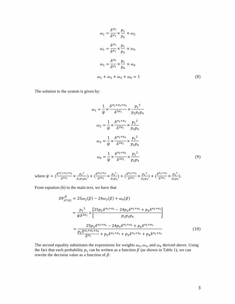
3

𝜔! =𝛿!!

𝛿!!×𝑝!𝑝!

× 𝜔!

𝜔! =𝛿!!

𝛿!!×𝑝!𝑝!

× 𝜔!

𝜔! =𝛿!!

𝛿!!×𝑝!𝑝!

× 𝜔!

𝜔! + 𝜔! + 𝜔! + 𝜔! = 1 (8)

The solution to the system is given by:

𝜔! =1𝜓×𝛿!!!!!!!!

𝛿!!!×

𝑝!!

𝑝!𝑝!𝑝!

𝜔! =1𝜓×𝛿!!!!!

𝛿!!!×𝑝!!

𝑝!𝑝!

𝜔! =1𝜓×𝛿!!!!!

𝛿!!!×𝑝!!

𝑝!𝑝!

𝜔! =1𝜓×𝛿!!!!!

𝛿!!!×𝑝!!

𝑝!𝑝! (9)

where 𝜓 = (!!!!!!!!!

!!!!× !!!

!!!!!!) + (!

!!!!!

!!!!× !!!

!!!!) + (!

!!!!!

!!!!× !!!

!!!!) + (!

!!!!!

!!!!× !!!

!!!!).

From equation (6) in the main text, we have that

𝐷𝑉!! !! = 25𝜔! 𝛽 − 24𝜔! 𝛽 + 𝜔! 𝛽

=𝑝!!

𝜓𝛿!!!×25𝑝!𝛿!!!!! − 24𝑝!𝛿!!!!! + 𝑝!𝛿!!!!!

𝑝!𝑝!𝑝!

=25𝑝!𝛿!!!!! − 24𝑝!𝛿!!!!! + 𝑝!𝛿!!!!!

𝑝!𝛿!!!!!!!!𝛿!! + 𝑝!𝛿!!!!! + 𝑝!𝛿!!!!! + 𝑝!𝛿!!!!!

(10)

The second equality substitutes the expressions for weights 𝜔!,𝜔!, and 𝜔! derived above. Using the fact that each probability 𝑝! can be written as a function 𝛽 (as shown in Table 1), we can rewrite the decision value as a function of 𝛽:

4

𝐷𝑉!!(!)! =

25(.66 − .66𝛽)𝛿!!!!! − 24(.67 − .66𝛽)𝛿!!!!! + (.66𝛽 − .33)𝛿!!!!!. 66𝛽𝛿!!!!!!!!

𝛿!! + (.66 − .66𝛽)𝛿!!!!! + (.67 − .66𝛽)𝛿!!!!! + (.66𝛽 − .33)𝛿!!!!!

Note that both the numerator and denominator are each linear functions of 𝛽, which implies that

the sign of !!"

!!(!)!

!" is independent of 𝛽. Thus, to show that 𝐷𝑉!!(!)

! decreases over 𝛽 ∈ !!, 1 , it is

sufficient to show that it decreases over any two points in this interval. We proceed by showing

that 𝐷𝑉!!(!)!! − 𝐷𝑉!!(!)

! > 0:

𝐷𝑉!! !!! − 𝐷𝑉!! !

!

=8.25𝛿!!!!! − 8.16𝛿!!!!!

0.33𝛿!!!!!!!!!!! + 0.33𝛿!!!!! + 0.34𝛿!!!!!

−0.33𝛿!!!!! − 0.24𝛿!!!!!

0.66𝛿!!!!!!!!!!! + 0.33𝛿!!!!! + 0.01𝛿!!!!!

=8.25𝛿!! − 8.16𝛿!!

0.33𝛿!!!!!!!! + 0.33𝛿!! + 0.34𝛿!! −0.33𝛿!! − 0.24𝛿!!

0.66𝛿!!!!!!!! + 0.33𝛿!! + 0.01𝛿!! (11)

If we denote the denominators in the first and second terms by 𝑑! and 𝑑!, respectively, we can

rewrite 𝐷𝑉!! !!! − 𝐷𝑉!! !

! as:

8.25𝛿!! − 8.16𝛿!! 𝑑! − 0.33𝛿!! − 0.24𝛿!! 𝑑!

𝑑! × 𝑑! (12)

Because both 𝑑! and 𝑑! are positive, it is sufficient to show that the numerator is positive:

8.25𝛿!! − 8.16𝛿!! 𝑑! − 0.33𝛿!! − 0.24𝛿!! 𝑑!= 𝛿!! 0.1617𝛿!! + 2.6136𝛿!! + 5.445𝛿!!!!!!!!

− 2.805𝛿!! + 5.3064𝛿!!!!!!!! + 0.1089𝛿!!!!!!!!

> 𝛿!! 0.1617𝛿!! + 2.6136𝛿!! + 5.445𝛿!!!!!!!!

− 2.805𝛿!! + 5.3064𝛿!!!!!!!! + 0.1089𝛿!!!!!

= 𝛿!! 0.1617𝛿!! + 2.6136𝛿!! + 5.445𝛿!!!!!

− 2.805𝛿!! + 5.3064𝛿!!!!! + 0.1089𝛿!!

= 𝛿!! 0.1617𝛿!! − 0.3003𝛿!! + 0.1386𝛿!!!!!

= 𝛿!! 𝑎𝛿!! + 𝑏𝛿!!!!! − 𝑎 + 𝑏 𝛿!! (13)

5

where the inequality follows from the fact that 1 > 𝛿 > 0 and 𝜎! > 𝜎! > 𝜎! = 0, and in the last equality, we define constants, 𝑎 = 0.1617 and 𝑏 = 0.1386. Furthermore, because 𝛿!! > 0, we need only show that the following expression is positive: 𝑎𝛿!! + 𝑏𝛿!!!!! − 𝑎 + 𝑏 𝛿!!

= 𝑎 𝛿!! − 𝛿!! − 𝑏𝛿!! 1 − 𝛿!!

> 𝑎 𝛿!! − 𝛿!! − 𝑎𝛿!! 1 − 𝛿!!

= 𝑎 (𝛿!! − 𝛿!!) − (𝛿!! − 𝛿!!!!!) (14)

Because 𝜎! + 𝜎! > 𝜎! > 𝜎!, and 𝑓 𝑥 = 𝛿! is decreasing and convex, we have that (𝛿!! −𝛿!!) > (𝛿!! − 𝛿!!!!!), which implies that the expression above is positive. ∎

B. Structural Estimation of Salience Model in Experiment 2

The goal of the structural estimation in experiment 2 is to estimate the salience function

from the choice data only. We then test whether the estimated salience function is correlated with

the eyetracking data. On each of the twenty-five trials, we assume the salience function is given

by 𝜎 𝑥!!, 𝑥!! = !!!!!!!

!!|!!! ! |!!!. The decision value of choosing the risky lottery, 𝑅, is defined by:

𝐷𝑉! = 𝜔!"#$ 𝑔 − 𝑐 + 𝜔!"##(𝑙 − 𝑐), where 𝜔!"#$ and 𝜔!"## denote the decision weights for the

gain and loss states, respectively. These weights are a function of (𝛿, 𝜃), and thus these are the

parameters we estimate with MLE.

We pool all subjects and trials, and estimate the two parameters at the group level. We

define 𝑧! = 1 if a subject chooses the risky lottery on trial t, and 𝑧! = 0 if a subject chooses the

certain option on trial t. We assume subjects exhibit stochastic choice, such that the probability of

choosing the risky lottery is a logistic function of the decision value of choosing the risky lottery:

𝑓 𝑧! 𝛿, 𝜃 ) = !

!!!!!"!! . We then maximize the following log likelihood function:

𝐿𝐿 𝛿, 𝜃 𝑧) = (𝑧!) log 𝑓 𝑧! 𝛿, 𝜃) + (1 − 𝑧!) log 1 − 𝑓 𝑧! 𝛿, 𝜃) (15)!"×!"

!!!

6

We find that the function is maximized at -766.45, and the best fitting parameters are, 𝛿, 𝜃 =

0.21, 0.05 .

1

Online Appendix for “THE ROLE OF SALIENCE AND ATTENTION IN CHOICE UNDER RISK: AN EXPERIMENTAL INVESTIGATION”

Cary Frydman and Milica Mormann

A. Basic Risk Choice Sets from Experiment 1 Section A.1. Basic Risk Choice Sets

After subject completed the four decision problems in the first experiment (Correlated

Allais paradox), we gave subjects an additional thirty-five questions to assess basic risk attitudes.

We refer to these questions as the Basic Risk Choice Sets. These questions are identical to those

used in the control condition of the visual salience experiment (Experiment 3). The only

difference is that these trials were incentivized, and because of the within subjects design, we are

able to test for the relationship between risk taking in the Correlated Allais questions and the

Basic Risk Choice Sets.

For each of the thirty-five trials, the subject chooses between a risky lottery and a certain

option. The risky lottery, 𝑅 = (𝑥, 𝑝; 𝑦, 1 − 𝑝) is a mean-preserving spread of the certain option,

𝐶 = 𝑐, 1 where 𝑥 > 𝑐 > 𝑦 ≥ 0 and 𝑝 ∈ 0,1 .There are thus two states of the world,

𝑠 ∈ {𝑔𝑎𝑖𝑛, 𝑙𝑜𝑠𝑠}. We define Pr 𝑆 = 𝑔𝑎𝑖𝑛 = 𝑝 because with probability 𝑝, the risky lottery

delivers a gain relative to the certain payoff, c. The parameter values for all thirty-five trials are

identical to those in Table 6.

Section A.2. Basic Risk Taking Results

Overall, subjects choose the risky lottery on 41.1% of trials in the Basic Risk Choice

Sets. Table A1.1 presents the average risk taking results disaggregated by trial, where each cell

corresponds to a different trial1. Each column characterizes the probability of the gain state and

each row characterizes the expected value of the risky lottery (and, by design, of the certain

option). The shaded cells correspond to those trials for which the gain state is salient.

Table A1.2 provides results from a regression of risk taking on economic salience. The

dependent variable is a dummy variable that takes on the value 1 if the subject chose the risky

lottery and EconSal is a dummy that takes on the value 1 if the gain state is salient. Column (1)

shows that subjects are significantly more likely to take risk when the gain state is salient (49.8%)

compared to when the loss state is salient (34.1%). Column (2) adds a subject fixed effect and the

1 Due to a software error, we failed to record data on one trial for thirty-three subjects (trial 32 in Table 6), and thus these trials are excluded from the subsequent analyses in this experiment.

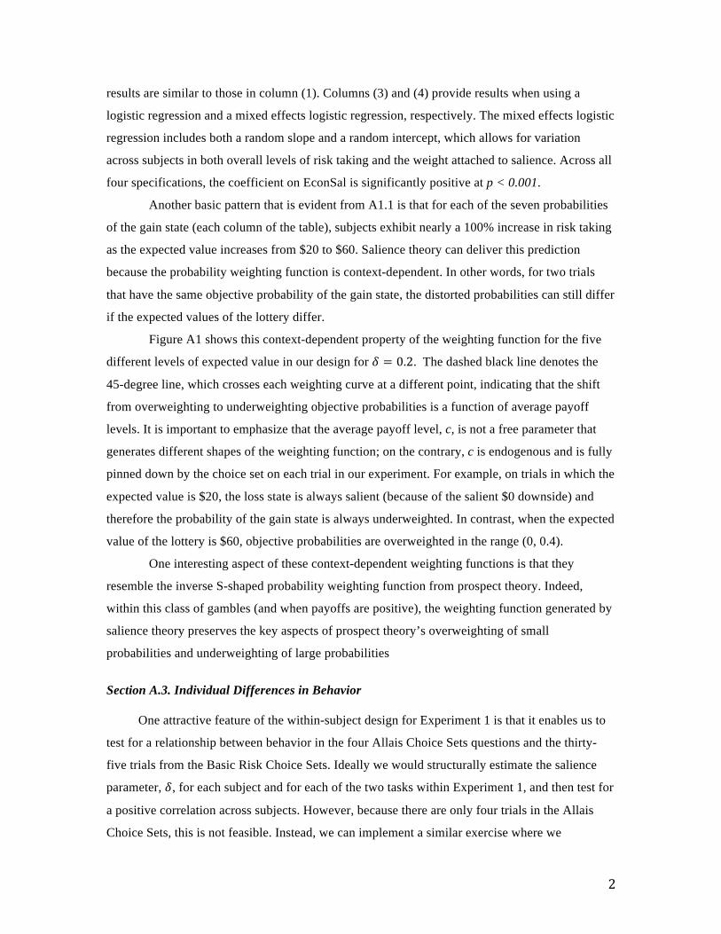
2

results are similar to those in column (1). Columns (3) and (4) provide results when using a

logistic regression and a mixed effects logistic regression, respectively. The mixed effects logistic

regression includes both a random slope and a random intercept, which allows for variation

across subjects in both overall levels of risk taking and the weight attached to salience. Across all

four specifications, the coefficient on EconSal is significantly positive at p < 0.001.

Another basic pattern that is evident from A1.1 is that for each of the seven probabilities

of the gain state (each column of the table), subjects exhibit nearly a 100% increase in risk taking

as the expected value increases from $20 to $60. Salience theory can deliver this prediction

because the probability weighting function is context-dependent. In other words, for two trials

that have the same objective probability of the gain state, the distorted probabilities can still differ

if the expected values of the lottery differ.

Figure A1 shows this context-dependent property of the weighting function for the five

different levels of expected value in our design for 𝛿 = 0.2. The dashed black line denotes the

45-degree line, which crosses each weighting curve at a different point, indicating that the shift

from overweighting to underweighting objective probabilities is a function of average payoff

levels. It is important to emphasize that the average payoff level, c, is not a free parameter that

generates different shapes of the weighting function; on the contrary, c is endogenous and is fully

pinned down by the choice set on each trial in our experiment. For example, on trials in which the

expected value is $20, the loss state is always salient (because of the salient $0 downside) and

therefore the probability of the gain state is always underweighted. In contrast, when the expected

value of the lottery is $60, objective probabilities are overweighted in the range (0, 0.4).

One interesting aspect of these context-dependent weighting functions is that they

resemble the inverse S-shaped probability weighting function from prospect theory. Indeed,

within this class of gambles (and when payoffs are positive), the weighting function generated by

salience theory preserves the key aspects of prospect theory’s overweighting of small

probabilities and underweighting of large probabilities

Section A.3. Individual Differences in Behavior One attractive feature of the within-subject design for Experiment 1 is that it enables us to

test for a relationship between behavior in the four Allais Choice Sets questions and the thirty-

five trials from the Basic Risk Choice Sets. Ideally we would structurally estimate the salience

parameter, 𝛿, for each subject and for each of the two tasks within Experiment 1, and then test for

a positive correlation across subjects. However, because there are only four trials in the Allais

Choice Sets, this is not feasible. Instead, we can implement a similar exercise where we

3

structurally estimate 𝛿 for each subject from the Basic Risk Choice sets, and then test whether

this explains variation across subjects in risk taking in the Allais Choice Sets.

We begin by estimating 𝛿 for each subject using maximum likelihood estimation over the

thirty-five trials in the Basic Risk Choice Sets. We define 𝑧! = 1 if the subject chooses the risky

lottery on trial t, and 𝑧! = 0 if the subject chooses the certain option on trial t. We assume

subjects exhibit stochastic choice, such that the probability of choosing the risky lottery is a

logistic function of the decision value of choosing the risky lottery: 𝑓(𝑧! | 𝛿) =!

!!!!!"! ! . We

then maximize the following log likelihood function:

𝐿𝐿 𝛿 𝑧) = (𝑧!) log 𝑓(𝑧! | 𝛿) + (1 − 𝑧!) log 1 − 𝑓(𝑧! | 𝛿)!"!!!

𝐷𝑉! is defined as in the main text, and we use the salience function in equation (2) and we set

𝜃 = 0.1. This procedure yields an estimate of 𝛿 for each subject i, which we denote 𝛿!. The

average estimated 𝛿 across subjects is 0.89, with a standard deviation of 0.162.

The next step in the exercise is to test whether the estimated 𝛿 from the Basic Risk

Choice Sets can explain risk taking in the Allais Choice Sets. From equation (6), we know that

the decision value of choosing lottery 𝐴! 𝑧 ,𝐷𝑉!!(!)! , is a function of 𝛿. Our key test is whether

the estimated decision value, 𝐷𝑉!!(!)! 𝛿 can explain across-subject variation in choosing lottery

𝐴! 𝑧 in the Allais Choice Sets.

To implement this test, we run regressions where the dependent variable is behavior from

the Allais Choice Sets task, and the independent variable is a function of behavior from the Basic

Risk Choice Sets task. Specifically, Table A2 shows results from an OLS regression where the

dependent variable takes on the value 1 if the subject chose 𝐴! 𝑧 , and 0 if the subject chose

𝐴! 𝑧 . The independent variable is the decision value of choosing 𝐴! 𝑧 conditional on the

subject specific 𝛿 (estimated from the Basic Risk Choice Sets) and the correlation structure and

common consequence from that trial. Observations are at the subject-trial level and we cluster

standard errors at the subject level. Column (1) shows that the estimated decision value is a strong

predictor of the decision to choose 𝐴! 𝑧 .

2 We find a substantial number of subjects for which 𝛿 = 1 (45% of subjects). Among the subset of subjects for whom we estimate 𝛿 < 1, the average 𝛿 = 0.8, but there is still substantial variation (standard deviation: 0.17).

4

However, because the independent variable, 𝐷𝑉!!(!)! 𝛿 varies with the correlation

structure, it is possible that the result in column (1) is not driven by variation in 𝛿, but is instead

driven by variation in the correlation structure across trials. For example, because the decision

value of choosing 𝐴! 𝑧 is larger in the zero correlation condition compared to the intermediate

correlation condition for all 𝛿, the result in column (1) can be obtained even in the absence of

individual differences in 𝛿.

To address this concern, we add dummy variables in column (2) to control for condition

effects. The coefficient on the decision value in column (2) is therefore identified using within

condition variation in risk taking (across subjects). We see that the result remains significant at

the 5% level, indicating that individual differences in 𝛿 from the Basic Risk Choice Sets can

explain variation in the Allais Paradox across correlation structures. Columns (3) and (4) repeat

the same analyses but use the subset of subjects who have an estimated 𝛿 < 1. We see that the

result remains significant in this subsample, suggesting that variation among those subjects with

𝛿 < 1 can still explain additional variation in risk taking behavior in the Allais Choice Sets.

In summary, the results in this section provide evidence for a connection between basic

risk attitudes and the propensity to exhibit the Allais Paradox. Salience theory predicts such a

correlation if there is heterogeneity in 𝛿 across the subject population. Can other theories generate

a similar prediction? Regret theory generates the predictions of the Correlated Allais Paradox

experiment and it can also generate the preference for positively skewed lotteries over a mean

preserving certain option, as we find in the Basic Risk Choice Sets. However, without an

additional assumption of diminishing sensitivity of the choiceless utility function, regret theory

cannot generate the increase in risk taking we find as average payoff levels rise. Therefore,

without additional assumptions, regret theory cannot generate the prediction that behavior is

correlated between the Allais Choice Sets and the Basic Risk Choice Sets.

B. Post-hoc test of the ordering property using eye tracking data

The results in Table 5 of the main text are inconsistent with the specific salience function

defined in (2). However, these regressions do not allow for a general test of the ordering and

diminishing sensitivity properties of the BGS salience function. While our experiment is not

optimized to provide tests of these general properties, we can exploit one feature of our design

that enables us to conduct a post-hoc test of the ordering property. Table 3 shows that there are

only five distinct loss states, (x!"##! , x!"##! ) ∈ { 0,10 , 5,15 , 10,20 , 15,25 , 20,30 }. For each

5

of these five loss states, there are five associated gain states, and we can rank the salience of each

of these five gain states according to the ordering property.

To see this, consider a general salience function, σ x!!! , x!!

! that satisfies ordering and

diminishing sensitivity. Now take the first loss state in our experiment, 0,10 , which corresponds

to the choice sets in the first five rows in Table 3. By ordering, we can rank the salience of the

five associated gain states into quintiles: σ 20,10 < σ 25,10 < σ 30,10 < σ 35,10 <

σ 40,10 . Because the loss state is fixed, we can also rank the salience difference between gain

and loss states into quintiles. We therefore predict that RelativeGainTime, should increase in

these quintiles. To test this, for each quintile we compute the average RelativeGainTime across

the five loss states, and we plot this in Figure A2. There is a weak monotonic relationship, but the

standard errors are too large to reject any difference in RelativeGainTime across any of the five

quintiles. If we collapse the data further into a “high” group (quintiles 4 and 5) and a “low” group

(quintiles 1 and 2), we do find that the difference in RelativeGainTime between the two groups is

positive and approaches a marginal level of significance (p = 0.109). As our experiment is not

designed to test the general property of ordering, one potential reason we fail to detect significant

differences is due to statistical power.

C. Comparing risk-taking in the incentivized laboratory experiment to risk-taking on mTurk

In this section we compare the behavior of subjects in the Basic Risk Choice Sets from

Experiment 1 to the behavior of subjects on mTurk (Experiment 3). We find that there is no major

qualitative difference in overall risk taking levels: subjects choose the risky lottery on 41.1% of

trials in the laboratory compared to 38.7% on mTurk.

We then formally compare, across the two samples, the degree to which subjects rely on

economic salience when making their decisions. Table A.3 provides evidence that there is no

systematic difference in the sensitivity to economic salience across those subjects who face the

Basic Risk Choice Sets in the laboratory, compared to those subjects who face the same choice

sets on mTurk (in the control condition). In Table A.3, mTurk is a dummy that takes on the value

1 if the subject is from mTurk. We see that neither the coefficient on mTurk, nor the coefficient

on the interaction between mTurk and EconSal is significantly different from zero. While this

analysis does not rule out the possibility that incentives can affect the visual salience treatment,

the fact that economic salience has a much larger effect on risk taking compared to visual salience

6

(Table 7) provides us with confidence that overall risk taking levels are unlikely to exhibit a

major qualitative shift if incentives were shifted.

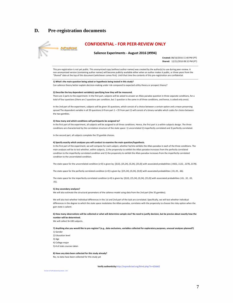
7

D. Pre-registration documents

����������3����� ���3���������

�����!����+#�%� �!'&�3��(�(&'�:89>�47AA<5�%��'��0�9A2:?2;9:?�::.=9���4��5

���%��0���:;2;:2;9:?�9A.<;���4��5

���$�!#�3#���$%#�%� ���$�� %�*�%�!&����/����$��� �*��+���� !*�4(�%� &%��&%� #�����$5�(�$��#��%����*�%����&%� #4$5�% �&$���&#����!��#3#�'��(/��� �3�� �*��+���'�#$� ��4� �%��������&%� #�����$5�(������� ���!&�����*��'����������%��#�(��������&%� #�����$��%�!&����-� #�%�#���*��#$��# ��%��0 ��#��1���%���%�%���% !� ��%��$�� �&���%�4(�����'�#�� ��$���#$%5/���%���%��%�%����%���� �%��%$� ��%��$�!#�3#���$%#�%� ���#��� ������%���/

95����'6&�'��� ��!�$(�&'�"!����!���&����"%��,#"'��&�&����!��'�&'����!�'��&�&'(�,.

����$��������%�� #*���%%�#��)!���������$� �3�������&���#�#�$��� �!�#���% ��)!��%���&%���%*�%�� #*� #�!# $!��%�%�� #*,

:5���&�%����'�����,���#�!��!'�)�%�����4&5�&#����,�!���"*�'��,�*������� ��&(%��1

���#���#��;�!�#%$�% �%����)!�#����%/����%�����#$%�!�#%-�$&����%$�(��������$����% ���$(�#���������$�!�#�� )�"&�$%� �����%�#���$�!�#�%��� ���%� �$-�� #��

% %��� ��� &#�"&�$%� �$�4%��#���#��;�"&�$%� �$�!�#�� ���%� �-��&%�:�"&�$%� ���$�%���$�����������%�#���� ���%� �$-����������-��$��$���� ��*� ���5/

���%���;���!�#%� ��%����)!�#����%-�$&����%$�(���������'���<>�"&�$%� �$-�(������ �$�$%� ������ ������%(��������#%���� !%� ������������3!#�$�#'���

$!#���/������!�����%�'�#�������������<B�"&�$%� �$�4=��# ��!�#%�:�C�<>��# ��!�#%�;5�(����� �$�$%� ��������#*�'�#������(������ ��$�� #��� ������%(���

%���%( �������$/

;5��"*� �!,��!��*������"!��'�"!&�*����#�%'���#�!'&�����&&��!���'".

���%�����#$%�!�#%� ��%����)!�#����%-�����$&����%$�(��������$$������% �����%�#���� ���%� �$/������-�%�����#$%�!�#%��$���(�%���3$&����%$���$���/�����%�#��

� ���%� �$��#�����#��%�#�+����*�%���� ##���%� ��$%#&�%&#�� ��%���$%�%��$!���.�:5�&�� ##���%���;5���!�#���%�*�� ##���%�������<5�!�#���%�*�� ##���%��/

���%���$�� ���!�#%-�����$&����%$�� �!��%��%���<>���������� ���$/

<5��#����,��+��'�,�*������!��,&�&�,"(�*�����"!�(�'�'"��+� �!��'��� ��!�$(�&'�"!2�,#"'��&�&1

���%�����#$%�!�#%� ��%����)!�#����%-�(��(����� �!&%��� #������$&����%-�(��%��#���2$����)����%$�%��������$�!�#�� )��������� ��%���%�#���� ���%� �$/����

���������*$�$�(�������% �%�$%�(��%��#-�(�%����$&����%$-�:5�%���!# !��$�%*�% ��)����%�%��������$�!�#�� )����#��$�$��# ��%���!�#���%�*�� ##���%��

� ���%� ��% �%�����!�#���%�*�� ##���%���� ���%� ������;5�%���!# !��$�%*�% ��)����%�%��������$�!�#�� )����#��$�$��# ��%�����!�#���%�*�� ##���%��

� ���%� ��% �%���&�� ##���%���� ���%� �/

����$%�%��$!����� #�%���&�� ##���%���� ���%� ��4+D95��$���'����*.�649-95-�4;>-;=5-�49-;=5-�4;>-957�(�%���$$ ���%���!# ������%��$�4/==;;-/::;;-�/;;@A-/;:@A5/

����$%�%��$!����� #�%���!�#���%�*�� ##���%���� ���%� ��4+D95��$���'����*.�64;>-;=5-�49-;=5-�49-957�(�%���$$ ���%���!# ������%��$�4/<<-/9:-�/??5/

����$%�%��$!����� #�%�����!�#���%�*�� ##���%���� ���%� ��4+D95��$���'����*.�649-95-�4;>-;=5-�49-;=5-�4;>-957�(�%���$$ ���%���!# ������%��$�4/?>-�/<;-�/9;-

/9:5/

=5��!,�&��"!��%,��!��,&�&.

���(������$ ��$%���%��%���$%#&�%&#���!�#���%�#$� ��%���$��������� ����&$������%���# ��%���;���!�#%�4%���<>�������$5/�

���(������$ �%�$%�(��%��#�����'��&��������#����$����%���:$%�����;���!�#%� ��%���%�$���#��� ##���%��/� !���������*-�(��(����%�$%�(��%��#�����'��&��

�����#����$����%������#���% �(�����%���$%�%��$!����� �&��%�$�%��������)�!�#�� )-�� ##���%�$�(�%��%���!# !��$�%*�% ��� $��%���#�$�*� !%� ��(����%��

�����$%�%���$�$�����%/

>5��"*� �!,�"�&�%)�'�"!&�*��������"����'���"%�*��'�*������'�% �!��&� #���&�-�.��"�!����'"��(&'��,�����&�"!/��('����#%���&����"('��+��'�,��"*�'��

!( ��%�*���������'�% �!��1

���(����� ����%�D:99�$&����%$/

?5��!,'��!����&��,"(�*"(��������'"�#%�3%���&'�%.�4�1�1/���'���+��(&�"!&/�)�%�����&��"����'����"%��+#�"%�'"%,�#(%#"&�&/�(!(&(����!��,&�&�#��!!��.5

:5������#

;5���&��%� ����'��

<5����

=5�� ��������� #

>5�8� ��$%�%$�� &#$�$�%����

@5���)���!,���'�����!��"����'����"%�'��&�&'(�,���%���,.

-�� ���%����'�������� ����%���� #�%��$�$%&�*�*�%

��%��,��('��!'���',0�%%!.22�$!#����%��/ #�2�����/!�!2,)D�;��?;�

��#$� �� ���$�#����%����&�$%� �$.�:/9>

8

����������3����� ���3���������

��'"��%�:89>���&(��������!����+#�%� �!'�479=9<5�%��'��0�983983:89>�8>/<=���5��6

���%��0���9:3:93:89>�8?/;;���5��6

���%�"$�4$���%&$�&�! ��%� !&�+�&�"'����0����%�� ! +��,����!"+�5)�&�!'&��'&�!$� ���%6�)�%��$��&����+�&����'&�!$5%6�&!�'%���'$� ��"��$4$�(��)0�� ! 4� ! +��,���(�$%�! �5�! &�� � ���'&�!$� ���%6�)�������!���"'�����+��(����������&��$�)�� �� ��'&�!$�����%��&�"'����.�!$�&�$���+��$%��$!��&��1���$��2���&���&�&���&!"�!��&��%��!�'�� &�5)�����(�$��!��%���$%&60�� &���&��&�&����&����! &� &%�!��&��%�"$�4$���%&$�&�! ��$���! ���� &���0

95����'6&�'��� ��!�$(�&'�"!����!���&����"%��,#"'��&�&����!��'�&'����!�'��&�&'(�,.

�!�%�(�%'���%���� ������%���! !����$�%�4&��� �-�� �"�$&��'��$.��!�%��&����%�$�%�4&��� ���%����' �&�! �!��)�����%&�&���%������(�%'���+�%���� &-

:5���&�%����'�����,���#�!��!'�)�%�����4&5�&#����,�!���"*�'��,�*������� ��&(%��1

�'����&%�)��������%����&!���!!%����&)�� �����$&�� �!"&�! �� ������� 4"$�%�$(� ��%"$����� �;=�&$���%0�������"� �� &�(�$�������%����� �$+�(�$�����

)������!��%�)��&��$�&���%'����&�&!!��&���$�%�+�!"&�! �!$� !&0

;5��"*� �!,��!��*������"!��'�"!&�*����#�%'���#�!'&�����&&��!���'".

���$���$��;��! ��&�! %.�� ��&����*"�$��� &�)����'%����)�&�� 4%'����&%���%�� 0

96��! &$!���! ��&�!

:6���� ��$��&�� &�

;6�!%%��$��&�� &�

� �&����! &$!���! ��&�! .������!��&���&)!�%&�&�%��%��#'���+�(�%'���+�%���� &�5��'��� ��!$� ����!�!$%��$���!' &�$���� ���60

� �&������ �&$��&�� &��! ��&�! .�&������ �%&�&��)������������(�%'���+�%���� &�5���� .���'��� ��!$� ���7�����$!' �7��!�!$%�)��������!' &�$���� ���60

� �&���!%%�&$��&�� &��! ��&�! .�&���!%%�%&�&��)������������(�%'���+�%���� &�5���� .���'��� ��!$� ���7�����$!' �7��!�!$%�)��������!' &�$���� ���60

<5��#����,��+��'�,�*������!��,&�&�,"(�*�����"!�(�'�'"��+� �!��'��� ��!�$(�&'�"!2�,#"'��&�&1

���)����&�%&�)��&��$�$�%��&��� ���%��$��&�$�� �&������ �&$��&�� &��! ��&�! ��!�"�$���&!�&����! &$!���! ��&�! 0

���)����&�%&�)��&��$�$�%��&��� ���%�%�����$�� �&����!%%�&$��&�� &��! ��&�! ��!�"�$���&!�&����! &$!���! ��&�! 0

=5��!,�&��"!��%,��!��,&�&.

���)�����%&���&��&���"�$���&�$%�!����7�'���%���� ��7��!���.�)������*&� �%�&����!$���!.��� ��!��.��������$�5:89:6��!����&!�� ��'���(�%'���%���� ��0

>5��"*� �!,�"�&�%)�'�"!&�*��������"����'���"%�*��'�*������'�% �!��&� #���&�-�.��"�!����'"��(&'��,�����&�"!/��('����#%���&����"('��+��'�,��"*�'��

!( ��%�*���������'�% �!��1

�@;88�%'����&%�)��������!����&���! ����,! ��'$�0

?5��!,'��!����&��,"(�*"(��������'"�#%�3%���&'�%.�4�1�1/���'���+��(&�"!&/�)�%�����&��"����'����"%��+#�"%�'"%,�#(%#"&�&/�(!(&(����!��,&�&�#��!!��.5

�!

@5���)���!,���'�����!��"����'����"%�'��&�&'(�,���%���,.

�!.� !���&����(����� ��!����&����!$�&��%�%&'�+�+�&

��%��,��('��!'���',0�&&"/33�%"$����&��0!$�3��� �0"�"3-*@�*<; *�

��$%�! �!���%�$����&��� '�%&�! %/�908=

9

E. Experimental Instructions E.1 Experimental Instructions and Practice Problem for Experiment 1

10

11

E.2 Experimental Instructions and Practice Problem for Experiment 2 Thank you for participating in this experiment on decision-making. For your participation, you have already earned $5, but depending on your decisions to the questions in the experiment, you will have the opportunity to earn more money. Basic Setup of the Questions The experiment consists of twenty-five different questions. An example of the type of question you will be asked is shown below in the pie chart. For each question, you will be asked to choose one of two gambles called “Option S” and “Option L.” The amount of money you win depends on which gamble you choose and which slice of the pie (LEFT or RIGHT) is randomly selected. There is an equal chance that each slice of the pie is selected (50% for the LEFT slice and 50% for the RIGHT slice).

In the above example, this means that if you chose “Option S” there is a 50% chance you earn $18 and a 50% chance you earn $10. If instead you chose “Option L” you would earn $15 no matter what, since the outcome for “Option L” is the same for both slices. At the end of the experiment, one of the twenty-five trials will be randomly selected by the computer and you will be paid according to your decision on that trial. The outcome of the gamble will be determined by a coin flip by the experimenter if you choose an option where the outcome differs across the two different slices. Entering Your Decision on the Computer During the experiment, your eye movements will be recorded by an electronic sensor. It is therefore very important to keep your head still as much as possible. In order to enter your decision on each trial, press the space bar and at the same time verbally say your answer “S” or “L”.

12

E.3 Experimental Instructions and Practice Problem for Experiment 3

13

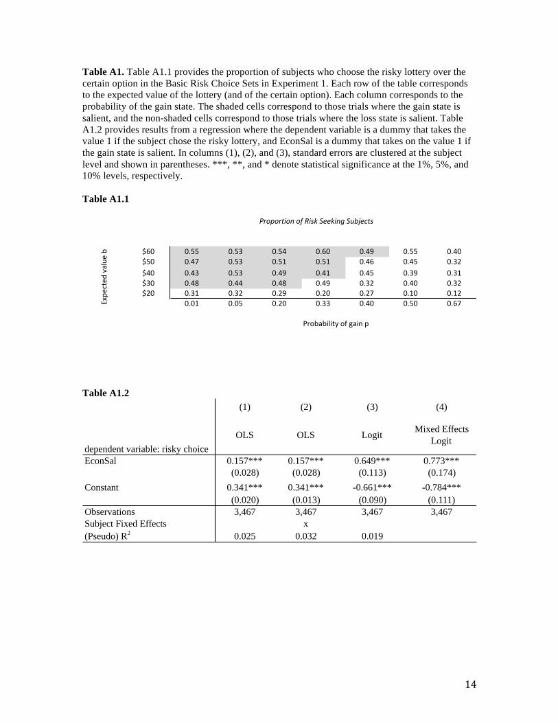
14

Table A1. Table A1.1 provides the proportion of subjects who choose the risky lottery over the certain option in the Basic Risk Choice Sets in Experiment 1. Each row of the table corresponds to the expected value of the lottery (and of the certain option). Each column corresponds to the probability of the gain state. The shaded cells correspond to those trials where the gain state is salient, and the non-shaded cells correspond to those trials where the loss state is salient. Table A1.2 provides results from a regression where the dependent variable is a dummy that takes the value 1 if the subject chose the risky lottery, and EconSal is a dummy that takes on the value 1 if the gain state is salient. In columns (1), (2), and (3), standard errors are clustered at the subject level and shown in parentheses. ***, **, and * denote statistical significance at the 1%, 5%, and 10% levels, respectively. Table A1.1

Table A1.2

ProportionofRiskSeekingSubjects

$60 0.55 0.53 0.54 0.60 0.49 0.55 0.40$50 0.47 0.53 0.51 0.51 0.46 0.45 0.32$40 0.43 0.53 0.49 0.41 0.45 0.39 0.31$30 0.48 0.44 0.48 0.49 0.32 0.40 0.32$20 0.31 0.32 0.29 0.20 0.27 0.10 0.12

0.01 0.05 0.20 0.33 0.40 0.50 0.67

ProbabilityofgainpExpe

cted

value

b

(1) (2) (3) (4)

dependent variable: risky choice

OLS OLS LogitMixed Effects

Logit

EconSal 0.157*** 0.157*** 0.649*** 0.773***(0.028) (0.028) (0.113) (0.174)

Constant 0.341*** 0.341*** -0.661*** -0.784***(0.020) (0.013) (0.090) (0.111)

Observations 3,467 3,467 3,467 3,467Subject Fixed Effects x(Pseudo) R2 0.025 0.032 0.019

15

Table A2. The table provides regressions where the dependent variable is a dummy that equals 1 if the subject chose 𝐴!(𝑧) in the Allais Choice Sets. Observations are at the subject-trial level. The variable estimated_DV is the decision value of choosing lottery 𝐴!(𝑧) conditional on the subject specific 𝛿 estimated from the Basic Risk Choice Sets. ZeroCorr, IntermediateCorr, and MaxCorrelation are condition dummy variables. The omitted category is the condition where z=24. Standard errors are clustered at the subject level. Columns (3) and (4) include only those subjects who have an estimate 𝛿<1 in the Basic Risk Choice Sets. ***, **, * denote statistical significance at the 1%, 5%, and 10% levels, respectively.

(1) (2) (3) (4)

dependent variable: chooseA1

OLS OLS OLS OLS

estimated_DV 0.569*** 0.306** 0.841*** 0.614***(0.147) (0.142) (0.218) (0.190)

ZeroCorr 0.399*** 0.360***(0.065) (0.089)

IntermediateCorr 0.309*** 0.343***(0.056) (0.075)

MaxCorr 0.100** 0.163**(0.044) (0.063)

Constant 0.273*** 0.086*** 0.313*** 0.103**(0.022) (0.030) (0.032) (0.042)

Observations 400 400 220 220R2 0.01 0.128 0.035 0.129

Full Sample Estimated Delta < 1

16

Table A3: Comparing risk taking results from the laboratory experiment and the mTurk experiment. EconSal is a dummy that takes on the value 1 if the gain state is economically salient. Mturk is a dummy that takes on the value 1 if the subject is from mTurk.

(1) (2)

dependent variable: risky choice

OLS Logit

EconSal 0.157*** 0.649***

(0.028) (0.113)

Mturk -0.036 -0.163

(0.026) (0.116)

EconSal*Mturk 0.018 0.092

(0.035) (0.142)

Constant 0.341*** -0.661***

(0.020) (0.090)Observations 6,938 6,938Subject Fixed Effects(Pseudo) R2 0.029 0.022

17

FIGURE A1: Context-Dependent Probability Weighting Function. The black dashed line is the 45-degree line. Each different colored line is the probability weighting function conditional on the average payoff level in the Basic Risk Choice Sets. The probability weights are generated

using 𝛿 = 0.2, the salience function, 𝜎 𝑥!! , 𝑥!! = !!!!!!!

!.!!|!!! ! |!!!, and the two properties that

characterize choice sets in the Basic Risk Choice Sets: 1) the choice set contains a risky lottery with a two-outcome support and a mean-preserving certain option and 2) the downside of the risky lottery is fixed at (c-20), where c denotes the payoff of the certain option.

0

0.2

0.4

0.6

0.8

1

0 0.2 0.4 0.6 0.8 1

Decision

Weight

Objec0veProbability

c=$20

c=$30

c=$40

c=$50

c=$60

18

FIGURE A2: Attention as a function of payoffs in Experiment 2. For a given loss state, each of its five associated gain states are ranked according to their salience. The bar chart plots the RelativeGainTime for each gain state quintile, averaged across each of the five loss states. Black bars denote standard errors (clustered at subject level). Each bar is significantly above zero at the 5% level, but no pairwise comparison between quintiles is significantly different from zero.

0

0.02

0.04

0.06

0.08

0.1

0.12

0.14

0.16

0.18

1 2 3 4 5

Rela%v

eGainT

ime

GainStateQuin%le