the role of reserves and anthropogenic habitats for
TRANSCRIPT
University of Nebraska - LincolnDigitalCommons@University of Nebraska - LincolnNebraska Cooperative Fish & Wildlife ResearchUnit -- Staff Publications
Nebraska Cooperative Fish & Wildlife ResearchUnit
2014
The role of reserves and anthropogenic habitats forfunctional connectivity and resilience of ephemeralwetlandsDaniel R. UdenUniversity of Nebraska-Lincoln, [email protected]
Michelle L. HellmanUniversity of Nebraska-Lincoln
David G. AngelerSwedish University of Agricultural Sciences, [email protected]
Craig R. AllenUniversity of Nebraska-Lincoln, [email protected]
Follow this and additional works at: http://digitalcommons.unl.edu/ncfwrustaff
This Article is brought to you for free and open access by the Nebraska Cooperative Fish & Wildlife Research Unit at DigitalCommons@University ofNebraska - Lincoln. It has been accepted for inclusion in Nebraska Cooperative Fish & Wildlife Research Unit -- Staff Publications by an authorizedadministrator of DigitalCommons@University of Nebraska - Lincoln.
Uden, Daniel R.; Hellman, Michelle L.; Angeler, David G.; and Allen, Craig R., "The role of reserves and anthropogenic habitats forfunctional connectivity and resilience of ephemeral wetlands" (2014). Nebraska Cooperative Fish & Wildlife Research Unit -- StaffPublications. 158.http://digitalcommons.unl.edu/ncfwrustaff/158

INVITED FEATURE: PROTECTED AREAS AS SOCIOECOLOGICAL SYSTEMS
Ecological Applications, 24(7), 2014, pp. 1569–1582� 2014 by the Ecological Society of America
The role of reserves and anthropogenic habitats for functionalconnectivity and resilience of ephemeral wetlands
DANIEL R. UDEN,1,4 MICHELLE L. HELLMAN,1 DAVID G. ANGELER,2 AND CRAIG R. ALLEN3
1Nebraska Cooperative Fish and Wildlife Research Unit, School of Natural Resources, 3310 Holdrege Street, University of Nebraska,Lincoln, Nebraska 68583 USA
2Swedish University of Agricultural Sciences, Department of Aquatic Sciences and Assessment, P.O. Box 7050,SE-750 07 Uppsala, Sweden
3U.S. Geological Survey, Nebraska Cooperative Fish and Wildlife Research Unit, School of Natural Resources, 3310 Holdrege Street,University of Nebraska, Lincoln, Nebraska 68583 USA
Abstract. Ecological reserves provide important wildlife habitat inmany landscapes, and thefunctional connectivity of reserves and other suitable habitat patches is crucial for the persistenceand resilience of spatially structured populations. To maintain or increase connectivity at spatialscales larger than individual patches, conservation actionsmay focus on creating andmaintainingreserves and/or influencing management on non-reserves. Using a graph-theoretic approach, weassessed the functional connectivity and spatial distribution of wetlands in the Rainwater Basinof Nebraska, USA, an intensively cultivated agricultural matrix, at four assumed, butecologically realistic, anuran dispersal distances. We compared connectivity in the currentlandscape to the historical landscape and putative future landscapes, and evaluated theimportance of individual and aggregated reserve and non-reserve wetlands for maintainingconnectivity. Connectivity was greatest in the historical landscape, where wetlands were also themost densely distributed. The construction of irrigation reuse pits for water storage hasmaintained connectivity in the current landscape by replacing destroyed wetlands, but these pitslikely provide suboptimal habitat. Also, because there are fewer total wetlands (i.e., wetlands andirrigation reuse pits) in the current landscape than the historical landscape, and because thedistribution of current wetlands is less clustered than that of historical wetlands, larger and longerdispersing, sometimes nonnative species may be favored over smaller, shorter dispersing speciesof conservation concern. Because of their relatively low number, wetland reserves do not affectconnectivity as greatly as non-reserve wetlands or irrigation reuse pits; however, they likelyprovide the highest quality anuran habitat. To improve future levels of resilience in this wetlandhabitat network, management could focus on continuing to improve the conservation status ofnon-reserve wetlands, restoring wetlands at spatial scales that promote movements of shorterdispersing species, and further scrutinizing irrigation reuse pit removal by considering effects onfunctional connectivity for anurans, an emblematic and threatened group of organisms.However, broader conservation plans will need to give consideration to other wetland-dependentspecies, incorporate invasive species management, and address additional challenges arising fromglobal change in social-ecological systems like the Rainwater Basin.
Key words: anurans; clustering; functional connectivity; graph theory; irrigation; modularity; ProtectedAreas as Socioecological Systems; Rainwater Basin, Nebraska, USA; resilience; restoration; wetlands.
INTRODUCTION
Deterministic changes in local environments that
steadily decrease wildlife population sizes and random
stochastic events that eliminate large numbers of
individuals may each contribute to local extinctions
(Atmar and Patterson 1993, Tscharntke et al. 2005,
Keith et al. 2008). The regional persistence of species is
facilitated by emigration and immigration of individuals
among patches of suitable habitat or the presence of
patches large enough to support multiple interacting
populations (Wahlberg et al. 1996, Gonzalez et al. 1998).
Manuscript received 17 September 2013; revised 2 January2014; accepted 23 January 2014. Corresponding Editor: E.Nelson.
Editor’s Note: Papers in this Invited Feature will bepublished individually, as soon as each paper is ready. Oncethe final paper is complete, a virtual table of contents withlinks to all the papers in the feature will be available at: www.esajournals.org/loi/ecap
4 E-mail: [email protected]
1569

Ecological reserves, defined here as lands set aside for
conservation purposes, provide wildlife with important
habitat patches in various landscapes.
Interspecific competition, species- and landscape-
specific dispersal components (e.g., dispersal probability,
dispersal distance, temporal dispersal patterns, disperser
mortality, and search time), and travel costs affect
successful colonization of suitable patches (Fahrig and
Merriam 1994, D’Eon et al. 2002, Belisle 2005). An
extinction threshold is crossed and extinction debt
created when the characteristics and/or arrangement of
habitat patches in an area no longer satisfy the
conditions necessary for the persistence of a population,
and without improvements, local extirpation becomes
inevitable (Atmar and Patterson 1993, Kareiva and
Wennergren 1995, Hanski and Ovaskainen 2002).
Metapopulations are characterized by the occasional
migration of individuals between habitat patches,
creating a balance between extinction and colonization
at larger spatial scales (Pulliam 2000). True metapopu-
lations carry high extinction risks for individual patches
and are relatively uncommon in nature; however, the
term usefully describes many spatially structured pop-
ulations (Fronhofer et al. 2012). The consideration of
genetically connected populations as metapopulations
and the promotion of functional connectivity among
habitat patches are important for conserving popula-
tions scattered among, or restricted to, isolated habitat
patches (Wahlberg et al. 1996, Gibbs 2000, Wiens 2002).
Connectivity within landscapes refers to functional
relationships between habitat patches that are derived
from their spatial distribution and the movement of
organisms among them (Fahrig and Merriam 1994,
With et al. 1997, Haig et al. 1998). Certain landscape
characteristics may encourage or discourage among
patch movements of species that interact with land-
scapes at different spatial scales (Taylor et al. 1993,
Tischendorf and Fahrig 2000, D’Eon et al. 2002). In
addition to the spatial aspects of habitat patches, their
quality for breeding, foraging, and refuge are important.
The availability of suitable habitat patches may be
limited in landscapes that have undergone significant
change (e.g., agricultural landscapes); therefore, ecolog-
ical reserves and other publicly or privately owned lands
may play important roles in the conservation of unique
biodiversity elements (Lindenmayer et al. 2006), and
more broadly, the provisioning of ecosystem goods and
services in landscapes modified by humans (Fischer et al.
2006). However, conservation efforts can be costly, and
the efficiency of protected areas for maintaining
imperiled populations may depend on suboptimal
habitat patches that are critical for facilitating dispersal
among higher quality patches (Urban and Keitt 2001).
Thus, explicit spatial modeling is useful for evaluating
the role of protected areas and other habitats in
providing the functional connectivity required for the
conservation of populations of conservation concern in
human-modified landscapes.
Connectivity and network analysis have emerged as
important tools for the study of complex adaptivesystems and their resilience in the face of perturbations.
A social-ecological system (SES) is a type of complex,adaptive system that links ecosystems and human
societies by considering their interactions and impactson one another (Cumming 2011). An SES perspective isrelevant in agricultural landscapes, where economic
interests can conflict with environmental conservationand necessitate complex management trade-offs (San-
chez-Carrillo and Angeler 2010). In addition to asymme-tries and information processing, network characteristics
are spatially relevant aspects of complexity (Norberg andCumming 2008). Network theory is useful for illustrating
how the position of a system within a network of othersystems, interactions among systems, system connectiv-
ity, and other network properties affect system functionunder varying internal and external conditions (Cum-
ming 2011). The spatial arrangement of system compo-nents and their connectivity can affect information
collection, exchange, and processing within a system,and network resilience has been described as the ability of
networks to withstand elimination of components whilestill maintaining connectivity (Cumming 2011). Inter-mediate levels of connectivity and modularity (i.e., a
network-level metric that measures the separation ofnetworks into smaller, connected clusters [Newman
2006]) are hypothesized to increase the resilience of SESs(Holling 2001, Gunderson and Holling 2002, Walker and
Salt 2006, Webb and Bodin 2008, Cumming 2011).In this study, we assessed the functional connectivity
and spatial distribution of wetlands in an intensiveagricultural landscape at four assumed, but ecologically
realistic, anuran dispersal distances to evaluate anurancommunity resilience (i.e., the resilience ‘‘of what’’
[Carpenter et al. 2001]) under historic, current, andputatively future conditions (i.e., the resilience ‘‘to
what’’), and evaluate the importance of reserve andnon-reserve wetlands and other man-made water bodies
for maintaining connectivity. Results may provideinsights into how changes in land use, specifically the
number and spatial arrangements of remnant, reserve,and anthropogenic wetlands (i.e., irrigation reuse pits),affect the functional connectivity and resilience of these
key habitats embedded in an agricultural matrix. Thisinformation is relevant for management and conserva-
tion of wetlands (Mitsch and Gosselink 2007) andunique semiaquatic biota, including anurans (Baillie et
al. 2004, Stuart et al. 2004, Cushman 2006).
MATERIALS AND METHODS
Study area
The Rainwater Basin is a 15 800-km2 watershed
consisting of all, or portions of, 21 counties of south–central Nebraska, USA (Fig. 1; LaGrange 2005). Thisintensively farmed landscape is dominated by maize
(Zea mays) and soybean (Glycine max) production, andwater is obtained from surface and groundwater sources
DANIEL R. UDEN ET AL.1570 Ecological ApplicationsVol. 24, No. 7

(Dunnigan et al. 2011). Soil surveys from the early 20th
century document the existence of as many as 1000
major (i.e., semipermanent) and 10 000 minor (i.e.,
seasonal or temporary) wetlands in the Rainwater Basin
at the time of European settlement, ,10% of which
remain today (Gersib 1991, Bishop and Vrtiska 2008).
Wetlands are classified as semipermanent, seasonal, or
temporary, according to hydric soil series, water
retention, and plant community composition (Gersib
et al. 1989, Gilbert 1989, Rainwater Basin Joint Venture
Public Lands Work Group 1994). Semipermanent wet-
lands are typically the largest and are inundated for the
longest durations, whereas the smaller seasonal and
temporary wetlands are generally inundated for shorter
durations (Gersib et al. 1989, Bishop and Vrtiska 2008).
During wetter periods, all three wetland types provide
reliable habitat, whereas only semipermanent wetlands
provide habitat during drier times (Gersib et al. 1989).
Wetland reserves are defined here as publicly and
privately owned wetland areas set aside for conservation
purposes, while non-reserve wetlands do not have a
specific conservation status. More than one-third of
existing wetland reserves are classified as semiperma-
nent.
Technological advances and agricultural intensifica-
tion during the 20th century resulted in wetland
destruction and degradation via draining, development,
culturally accelerated sediment accumulation, conver-
sion to agriculture, and excavation for the construction
of irrigation reuse pits (Gersib 1991, LaGrange et al.
2011). Irrigation reuse pits (hereafter referred to as pits)
are typically situated at the lowest elevations on
properties and concentrate excess irrigation water runoff
for future use, and negatively impact hydroperiods
within watersheds by catching precipitation runoff that
might otherwise fill wetlands (LaGrange 2005). The
characteristics of pits are markedly different from those
of natural wetlands, with pits having greater depth,
steeper sides, greater and faster water-level fluctuations
during the irrigation season, and increased exposure to
irrigation runoff, and potentially, agricultural chemicals
(Stutheit et al. 2004, Grosse and Bishop 2012). These
characteristics may inhibit the growth of aquatic
vegetation in pits, which provides important anuran
breeding habitat, and likely decrease the value of pits as
wildlife habitat in general, despite the fact that pits tend
to hold water for longer durations than many wetlands
(Haukos and Smith 2003, Smith 2003, Stutheit et al.
2004, LaGrange 2005). All wetland, pit, and reserve
geographic information system (GIS) data used in this
study were georeferenced and provided by the Rain-
water Basin Joint Venture (more information available
online).5
Evaluating functional connectivity
We employed a graph-theoretic approach to assess the
functional connectivity of anuran habitats in historic,
current, and putative future scenarios of the Rainwater
Basin wetlands landscape. The wetlands landscape may
be substantially altered in the future through the global
change-mediated loss of reserve and non-reserve wet-
lands and/or the planned removal of pits. Therefore, we
considered the following range of landscape scenarios
FIG. 1. Location of the Rainwater Basin region in south–central Nebraska, USA, with current reserve and non-reserve wetlandlocations, major streams, and Nebraska counties displayed.
5 http://rwbjv.org/
October 2014 1571PROTECTED AREAS AS SOCIOECOLOGICAL SYSTEMS

that encompass possible future functional connectivity
patterns, based on current wetland distributions: current
wetlands excluding reserves, current wetlands excluding
pits, current wetlands excluding both reserves and pits,
and current wetland reserves excluding pits and non-
reserve wetlands. These potential future landscape
scenarios were compared with one another, as well as
with the historical and current scenarios of the land-
scape, resulting in six total landscape scenarios. The
relative density of wetlands in each landscape scenario
was examined with the average nearest neighbor
distance tool in ArcGIS, which uses a z test to compare
the observed mean distance between points with the
expected mean distance between the points, assuming a
random distribution of the points in the same area
(ESRI 2011).
When dispersal distances of target species are
unknown or uncertain, comparing the level of con-
nectivity among several nested spatial scales is useful for
gaining information about the effects of scale on
network-specific connectivity (Calabrese and Fagan
2004). Nine anuran species are known to occur in the
Rainwater Basin (Table 1). Because limited information
was available concerning the dispersal capabilities of
these particular species, we assumed four dispersal
distances that represent a range of their dispersal
potentials in rowcrop fields: 0.50, 1.00, 1.50, and 2.00
km. The maximum value of this range is nearly identical
to the reported mean maximum dispersal distance of
anurans (i.e., 2.02 km) in a variety of landscapes (Smith
and Green 2005); therefore, the dispersal potentials of
Rainwater Basin anurans are likely to lie within it.
In a graph-theoretic approach, individual habitat
patches are represented as nodes, and the connections
between them (i.e., Euclidian distances) as edges (Bunn
et al. 2000, Urban and Keitt 2001, Calabrese and Fagan
2004, Estrada and Bodin 2008). The term network is
used to describe the combination of all nodes and edges,
including those that are isolated or separated from one
another, and the term cluster refers to groups of
connected nodes within a specified distance, with �1cluster(s) constituting the larger network. Within net-
works, paths are defined as �1 edge between any unique
set of nodes that does not cross any one node more than
once (Bunn et al. 2000, Pascual-Hortal and Saura 2006).
Wetland networks for the six scenarios of the Rain-
water Basin wetlands landscape were built and analyzed
using ArcGIS and the program R (R Development Core
Team 2012), with R functions housed in the rgdal
(Bivand et al. 2013), sp (Bivand et al. 2008), SDMTools
(VanDerWal et al. 2012), and igraph (Csardi and
Nepusz 2006) packages. For each landscape scenario,
we converted individual water bodies to point features in
ArcGIS, using the geographic coordinates of the
location nearest the wetland centroid that was still
within the wetland polygon. In R, Euclidian distances
between each wetland centroid and every other wetland
centroid in the network were calculated, and connec-
tions with distances less than or equal to each of the four
dispersal distances were retained and used to create lists
of edges representing connections between wetland
nodes. Wetland nodes and edges were then combined
to produce a network for each landscape scenario at
each of the four dispersal distances (Fig. 2). Anurans,
like many other species, are unlikely to traverse
landscapes in straight lines; therefore, true dispersal
distances between wetlands may be underrepresented.
However, because information related to specific dis-
persal patterns for many organisms are unavailable
(Jacobson and Peres-Neto 2010), including anuran
movements in the Rainwater Basin, we used Euclidian
distance between sites as a best estimate. Euclidean
distance is commonly used in metacommunity studies as
a spatial proxy of connectivity and dispersal (Legendre
et al. 2005, Baldissera et al. 2012, Angeler et al. 2013).
Furthermore, because we lacked information related to
the directional movement of anurans in the landscape,
we assumed between-node travel to be random (i.e.,
undirected).
A variety of methods and metrics have been proposed
for examining node- and network-level connectivity, and
for determining the contributions of individual nodes to
network-level connectivity (Calabrese and Fagan 2004,
Pascual-Hortal and Saura 2006, Saura and Rubio 2010).
TABLE 1. Nine anuran species occurring in the Rainwater Basin, Nebraska, USA.
Species SVL (mm) Nonbreeding habitat
American bullfrog (Lithobates catesbeiana) 105–190� aquaticWoodhouse’s toad (Anaxyrus woodhousii) 58–113� terrestrialNorthern leopard frog (Lithobates pipiens) 55–95� semiaquaticPlains leopard frog (Lithobates blairi) 50–95� semiaquaticGreat Plains toad (Anaxyrus cognatus) 52–78� terrestrialPlains spadefoot toad (Spea bombifrons) 41–58� terrestrialGrey treefrog (Hyla chrysoscelis) 31–50� arborealWestern chorus frog (Psuedacris triseriata) 18–34� semiterrestrialNorthern cricket frog (Acris crepitans) 14–32� semiterrestrial
Notes: Dispersal ability is typically contingent on snout–vent length (SVL) and dependence onstanding water. All anurans require standing water during the breeding season; therefore,dependence on standing water is best indicated by the nonbreeding habitat of a species.
� Source is Ballinger et al. 2010.� Source is Lynch 1985.
DANIEL R. UDEN ET AL.1572 Ecological ApplicationsVol. 24, No. 7
We assessed node-level connectivity with degree central-
ity, which is simply the number of direct connections a
node maintains with adjacent nodes (Estrada 2007,
Estrada and Bodin 2008). The importance of individual
nodes for overall network connectivity was also
determined by sequentially removing each node from
the network, calculating the mean degree centrality
among the remaining nodes, and then replacing it before
repeating the process. To visually represent the spatial
distribution of node-level connectivity, we produced
continuous inverse distance weighted (IDW) raster
surfaces for interpolating degree centrality values among
nodes. Species occupying a habitat patch (i.e., node)
with a high degree centrality may emigrate to various
neighboring patches in the event that the patch they are
occupying becomes unsuitable as habitat. Similarly, if a
local extinction occurs in a patch with a high degree
centrality, species from neighboring patches may immi-
grate to recolonize it.
Network-level connectivity, which has been identified
as a determinant of system resilience (Holling 2001,
Gunderson and Holling 2002, Walker and Salt 2006,
Cumming 2011), was evaluated according to mean
degree centrality, the total number of clusters in the
network, the mean number of nodes composing clusters,
the percentage of total nodes contained in the largest
cluster, and a network modularity score. The more
distinct clusters of connected habitat patches that exist
in a network, the more disconnected the patches and the
species inhabiting them become, with the maximum
possible number of clusters being equal to the total
number of patches. Alternatively, the greater the
percentage of total patches that are contained in the
single largest cluster, the more patches in the network a
species can reach from any given patch within that
cluster, until connectivity increases to the point that the
entire network consists of a single cluster and any given
patch can be directly or indirectly reached from any
other patch. Therefore, habitat networks with fewer, but
larger and more encompassing, clusters provide species
with the greatest opportunities for movement through-
out the network. Although high levels of connectivity
maximize the potential for among-patch movement and
the resulting exchange of genetic information within
metapopulations, it may also facilitate biological in-
vasions and the spread of disease and other detrimental
elements through habitat networks and spatially struc-
tured populations. Modularity is a network-level metric
that measures the separation of networks into smaller
connected clusters and is greatest in networks where
connections are dense within clusters and sparse between
them (Newman 2006). Habitat networks with inter-
mediate levels of connectivity and modularity are
hypothesized to permit the movement of species among
patches and clusters, while still restricting detrimental
events to individual clusters, thereby minimizing the
potential for their spread through, and negative effect
on, the larger network (Ash and Newth 2007, Webb and
Bodin 2008).
RESULTS
Landscape scenario comparisons
Functional connectivity.—Of the six compared scenar-
ios of the Rainwater Basin landscape, the historical
wetlands landscape had the most wetlands, the densest
distribution of wetlands (Table 2), the greatest mean
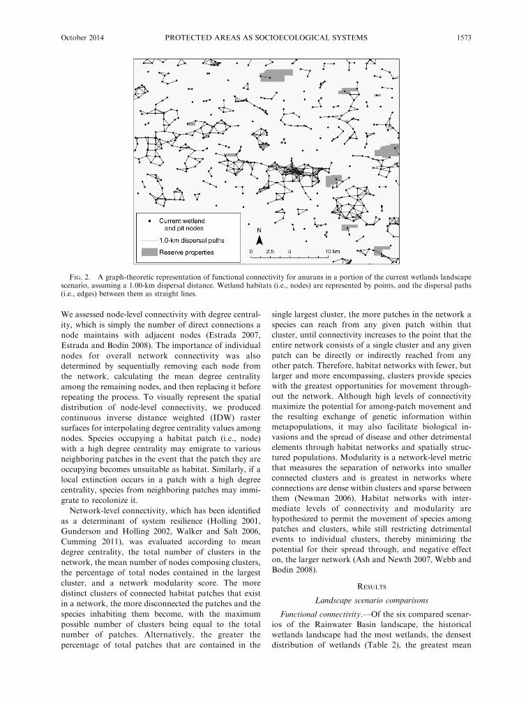
FIG. 2. A graph-theoretic representation of functional connectivity for anurans in a portion of the current wetlands landscapescenario, assuming a 1.00-km dispersal distance. Wetland habitats (i.e., nodes) are represented by points, and the dispersal paths(i.e., edges) between them as straight lines.
October 2014 1573PROTECTED AREAS AS SOCIOECOLOGICAL SYSTEMS

FIG. 3. Connectivity metrics among the six landscape scenarios at four assumed anuran dispersal distances. (a) Wetland degree(i.e., the number of direct connections a wetland has with other wetlands); (b) the mean number of wetlands per cluster; (c)modularity scores (i.e., the level of within- and between-cluster connectivity); (d) the number of wetland clusters in the entirenetwork; and (e) the percentage of wetlands in the largest cluster.
TABLE 2. Spatial clustering of wetlands in the six wetland landscape scenarios.
Landscape scenario No. wets ExpDist ObsDist DistDiff z P
Historical 11 711 808.90 482.07 326.83 �83.65 ,0.01Current 10 161 872.53 590.52 282.00 �62.33 ,0.01Current without reserves 9910 883.51 591.55 291.95 �62.93 ,0.01Current without pits 1856 1800.62 1093.92 706.70 �32.35 ,0.01Current without pits or reserves 1615 1912.91 1133.76 779.16 �31.31 ,0.01Reserves without pits or non-reserves 241� 4658.91 2294.31 2364.60 �15.07 ,0.01
Notes: For each scenario, a z score was calculated for comparing the observed mean distance between wetlands to the expectedmean distance between them, if their distribution is assumed to be random and in the same area. The P value represents theprobability that the null hypothesis (i.e., wetlands are randomly distributed) is true. Wetlands in all six scenarios were significantlyclustered, with lower z scores indicating more clustering. Analysis was conducted with the average nearest neighbor tool in ArcGIS(ESRI 2011). No. wets is the total number of wetlands in the landscape scenario; ExpDist is the expected mean distance betweenwetland centroids, in meters, assuming a random distribution of points; ObsDist is the observed mean distance between wetlandcentroids, in meters; and DistDiff is the difference in expected and observed mean distances between wetland centroids, in meters.
� A mismatch exists between the total number of current wetlands, the number of current wetlands without reserves, and thenumber of reserves without irrigation reuse pits or non-reserve wetlands, because of the fact that 10 pits are located on reserveproperties.
DANIEL R. UDEN ET AL.1574 Ecological ApplicationsVol. 24, No. 7

degree centrality, and the greatest mean number of
wetlands per cluster at each of the four dispersal
distances (Fig. 3a, b), indicating the greatest level of
overall connectivity. The historical landscape scenario
also had the highest modularity score at all four
dispersal distances (Fig. 3c). Following the historical
landscape scenario, connectivity for the current land-
scape scenario was . the current landscape excluding
reserves scenario, which was . the current landscape
excluding pits scenario, which was . the current
landscape excluding pits and reserves scenario, which
was . reserves excluding pits and non-reserve wetlands
scenario. Although exceptions to this ranking occurred
at several connectivity metric–landscape scenario–dis-
persal distance combinations, the ranking describes the
general pattern in connectivity among landscape scenar-
ios and dispersal distances, and highlights the contribu-
tions of reserve wetlands, non-reserve wetlands, and pits
to functional connectivity for anurans in the current,
and potentially future, wetlands landscapes.
Wetland spatial distributions.—The spatial distribu-
tions of wetlands in the historical, current, and future
landscape scenarios were all significantly clustered (i.e.,
the observed mean distance between wetlands was
significantly greater than the expected mean distance
between them, assuming their random distribution in the
same area); however, the distribution of wetlands was
most dense in the historical landscape scenario and least
dense in the reserves without pits and non-reserve
wetlands landscape scenario (Table 2). Although there
was a similar, but greater, number of wetlands in the
historical landscape scenario than the current landscape
scenario (Table 2), there were fewer wetland clusters in
the historical landscape scenario at each dispersal
distance (Fig. 3d), and accordingly, the mean number
of wetlands per cluster was greater in the historical
landscape scenario at each dispersal distance (Fig. 3b).
The exclusion of pits from the current landscape
scenario resulted in a noticeable decrease in wetland
density (Table 2).
Differences in wetland distributions and densities
among landscape scenarios and dispersal distances were
also evident from comparisons of wetland degree
centrality hotspot maps (Figs. 4–6). As expected,
among-wetland connectivity tended to be greater in
landscape scenarios with more wetlands and at greater
dispersal distances. More localized areas of relatively
high among-wetland connectivity were present in the
historical wetlands landscape scenario than in the
current wetlands landscape scenario or the current
wetlands excluding pits landscape scenario. Further-
more, the current wetlands landscape scenario tended to
contain more, and more uniformly-distributed, areas
with moderate levels of among-wetland connectivity
FIG. 4. Inverse distance weighted continuous raster surface of wetland degree centrality in the historical wetlands landscapescenario at the (a) 0.50-km, (b) 1.00-km, (c) 1.50-km, and (d) 2.00-km dispersal distances. Wetland degree centrality refers to thenumber of direct connections between a wetland and other wetlands, and wetlands in darker shaded areas tend to be moreconnected.
October 2014 1575PROTECTED AREAS AS SOCIOECOLOGICAL SYSTEMS

than the historical landscape scenario. Although the
current wetlands excluding pits landscape scenario
displayed lower overall levels of connectivity than the
historical or current landscape scenarios, hotspots of
connectivity within it still appeared to be more localized
than in the current wetlands landscape scenario.
Dispersal distance connectivity thresholds.—Function-
al connectivity was affected by dispersal distance, and
dramatic shifts in network-wide connectivity in different
landscape scenarios were detected between certain
dispersal distances. For example, in the historical
landscape scenario, the percentage of total wetlands in
the largest cluster increased from 1.8% to 88.4% between
the 0.50- and 1.00-km dispersal distances, and then more
gradually increased to 97.9% total inclusion at the 2.00-
km dispersal distance (Fig. 3e), indicating a dispersal
threshold between 0.50 and 1.00 km, where the majority
of wetlands were all directly or indirectly connected with
one another. A more gradual increase in connectivity
was evident in the current landscape scenario, where the
percentage of wetlands in the largest cluster increased
from ,0.1% to 58.7% between the 0.50- and 1.00-km
dispersal distances, and then to 85.7% and 95.2% at
1.50- and 2.00-km dispersal distances, respectively (Fig.
3e), making any connectivity thresholds less apparent.
In the current landscape scenario without pits, the
greatest increase in the percentage of wetlands in the
largest cluster occurred between the 1.50- and 2.00-km
dispersal distances, with 73.9% of all wetlands being in
the largest cluster; however, only 26.1% of wetlands
were in the largest cluster in the reserves without pits
and non-reserves landscape scenario at the 2.00-km
dispersal distance (Fig. 3e).
Node contributions to connectivity
Specific wetland nodes that contributed most to
connectivity varied with the landscape scenario and
dispersal distance considered; however, some general
trends in their spatial distributions and statuses as
natural wetlands, pits, and reserves were evident. In the
historical landscape scenario, at dispersal distances
�1.00 km, all but one of the top 10 wetland contributors
to mean degree centrality were located within ;20 km of
one another in two portions of the same wetland cluster
(Fig. 7). In the current landscape scenario, wetlands in
this area are less dense, more uniformly distributed, and
consist primarily of pits. In fact, at each of the four
dispersal distances, the number of the top 10 historical
landscape scenario contributors to mean degree central-
ity that are still in existence today is 1, 2, 0, and 0,
respectively; and none of these are presently reserves.
In the current landscape scenario, at dispersal
distances �1.00 km, the majority of the top 10
contributors to mean degree centrality were located
FIG. 5. Inverse distance weighted continuous raster surface of wetland degree centrality in the current wetlands landscapescenario at the (a) 0.50-km, (b) 1.00-km, (c) 1.50-km, and (d) 2.00-km dispersal distances. Wetland degree centrality refers to thenumber of direct connections between a wetland and other wetlands, and wetlands in darker-shaded areas tend to be moreconnected.
DANIEL R. UDEN ET AL.1576 Ecological ApplicationsVol. 24, No. 7

.40 km to the southwest of the top contributors in the
historical landscape scenario (Fig. 8). Furthermore, the
number of these 10 in the current landscape that are
natural wetlands (i.e., not pits) at the four dispersal
distances is 0, 6, 10, and 10, respectively; and none are
presently reserves. In the current landscape without pits
scenario, at all four dispersal distances, all but one of the
top 10 contributors to mean degree centrality are
situated in the same wetland cluster as the top
contributors in the current landscape scenario (Fig. 9),
with the single isolated contributor at the 0.50-km
dispersal distance being a reserve.
DISCUSSION
The current wetlands landscape scenario of the
Rainwater Basin, in addition to four putative future
scenarios of it, all exhibited lower levels of functional
connectivity, modularity, and spatial wetland clustering
for anurans than the historical wetlands landscape
scenario. Thus, management action is required to
enhance the future sustainability of wetland networks
in the Rainwater Basin and similar agricultural land-
scapes. Important information for increasing the func-
tional connectivity of wetland landscapes in these areas,
and maintaining resilient anuran communities within
them, can be derived from our results. Because this
study evaluated functional connectivity of wetlands in
historic, current, and future scenarios of the wetland
landscape, it provides insights not only into how the
spatial arrangement and connectivity of habitat patches
may be influencing anuran species with different
dispersal abilities presently, but also as to how those
influences may have changed over the past century, and
may again in the future.
Relative hotspots of connectivity are apparent in the
different landscape scenario–dispersal distance combi-
nations (Figs. 4–6). Areas that had the highest levels of
connectivity historically are not only less connected
today, but are also less connected than other areas of the
current landscape, especially when pits are excluded.
The overall distribution of wetlands in the current
landscape is less dense than it was historically, even
though the number of wetland nodes in the historical
and current landscape scenarios is similar (Table 2). The
fact that pits are situated in agricultural fields that are
typically divided into square ;64-ha properties (Mitch-
ell et al. 2012) could contribute to this more uniform
distribution.
Most of the top 10 wetlands contributing to mean
degree centrality in the historical wetlands landscape
scenario at each dispersal distance have been lost, and as
the distribution of wetlands in the landscape changed,
the relative importance of specific wetlands for main-
taining mean degree centrality shifted. Following Euro-
FIG. 6. Inverse distance weighted continuous raster surface of wetland degree centrality in the current wetlands withoutirrigation pits landscape scenario at the (a) 0.50-km, (b) 1.00-km, (c) 1.50-km, and (d) 2.00-km dispersal distances. Wetland degreecentrality refers to the number of direct connections between a wetland and other wetlands, and wetlands in darker shaded areastend to be more connected.
October 2014 1577PROTECTED AREAS AS SOCIOECOLOGICAL SYSTEMS

pean settlement, connectivity in the Rainwater Basin
decreased via agricultural land use change, a stressor
that threatens the ecological integrity of wetlands
worldwide (Mitsch and Gosselink 2007). More than
9000 artificial water bodies (i.e., pits) have been
constructed with the main purpose of agricultural
irrigation, rather than environmental conservation, and
because of differences between them and natural wet-
lands (e.g., greater depth, steeper sides, greater water-
level fluctuations associated with irrigation practices
rather than natural meteorological phenomena, more
agricultural chemicals, and less aquatic vegetation),
these may provide suboptimal anuran habitat. Indeed,
previous research has shown that the presence of pits
does not improve the regional occurrence of anurans in
a boreal landscape (Anderson et al. 1999). Also,
irrigation pits may alter hydrological disturbance
regimes, negatively affecting natural wetlands. Our
results show that the construction of pits did not
compensate for the loss of natural wetlands in the area,
as connectivity was not restored to its former level.
Although our results suggest that the use of pits as
stepping stones for anuran dispersal may be limited, the
analysis of four dispersal distances, in combination with
the spatial distribution of pits, allows us to make
broader inferences about the importance of artificial vs.
natural water bodies for anurans. Although a large
proportion of wetlands in the historical wetlands land-
scape scenario were connected as a single cluster at a
1.00-km dispersal distance, the current wetlands land-
scape scenario only obtains the same percentage of
single-cluster connectivity at dispersal distances .1.50
km (Fig. 3e). Furthermore, many of the most critical
wetland nodes for maintaining mean degree centrality in
the current landscape scenario at dispersal distances
,1.00 km are pits, whereas natural wetlands become
more important at dispersal distances �1.00 km.
Therefore, post-European settlement changes in net-
work-level connectivity may be favoring larger, longer
distance dispersers (e.g., American bullfrog and plains
leopard frog) over smaller, shorter distance dispersers
(e.g., northern cricket frog). The cricket frog, small
bodied and short lived, is in decline in much of its range
and is listed as endangered in the States of Minnesota,
Wisconsin, and New York, and as a species of concern
in Indiana, Michigan, and West Virginia (Lanoo 2005).
Cricket frogs are reported to live an average of four
months, and may experience population turnover in as
few as 18 months (Burkett 1984). A well-connected
landscape that allows for dispersal to suitable wetlands
under a variety of climatic conditions is important for
the local persistence of cricket frogs and other short-
FIG. 7. Historical wetland nodes, together with the top 10 wetland contributors to mean network degree centrality at fouranuran dispersal distances (stars). (a) At the 0.50-km dispersal distance, the top contributors to degree centrality are more evenlydistributed throughout the region than at the (b) 1.00-km, (c) 1.50-km, and (d) 2.00-km dispersal distances, where all but one of thecontributors are located near one another in two portions of the same wetlands cluster. The numbers in panels (b), (c), and (d)correspond to the number of the top 10 contributors in specific vicinities.
DANIEL R. UDEN ET AL.1578 Ecological ApplicationsVol. 24, No. 7

distance dispersers, which may have been able to move
freely throughout the historical wetlands landscape, but
now are more restricted to intact clusters, with inter-
cluster movements limited. In addition to species-specific
dispersal abilities, it is important to consider the invasive
status of anurans. For example, the bullfrog is a
nonindigenous species that may prey upon, or out-
compete, other frog species (Werner et al. 1995, Adams
1999). Thus, a landscape that facilitates bullfrog
dispersal while impeding short-distance dispersal could
further threaten persistence of smaller species that are
already in peril.
Reserves play an important role in biodiversity
conservation (Lindenmayer et al. 2006). Many wetland
reserves in the Rainwater Basin that have best retained
natural hydroperiods and flood frequency regimes, and
thus ecological integrity, are large, semipermanent
wetlands. These reserves may be the most suitable
sources of anuran habitat; however, when considered in
isolation, they contribute less to network-level connec-
tivity than non-reserve wetlands or pits. This lower level
of connectivity among reserves is likely a result of only
;2.4% of water bodies in the current wetlands landscape
being reserves. Thus, the spatial isolation and low
number of wetland reserves may currently represent
two impediments toward an efficient use of wetland
reserves for conserving important biodiversity elements
like anurans. Non-reserve wetlands and other unmapped
temporary water bodies (e.g., temporarily flooded road
ditches, pools of irrigation runoff, and so on) may also
be important for maintaining connectivity, and could
serve as important stepping stones between more
permanent water bodies.
Resilience has been defined as the ability of a system
to absorb disturbances without fundamentally altering
its structures and functions (Holling 1973). However,
when disturbance thresholds are exceeded, a system tips
into an alternative state and rearranges around a new set
of processes, structures, and feedbacks. The historical
wetlands landscape of the Rainwater Basin had the
highest levels of connectivity and modularity, and likely
allowed anurans to spread across it, using suboptimal
habitats as stepping stones for accessing higher quality
sites. These spatial processes may have played a major
role in maintaining structural and functional attributes
of anuran communities, and likely conferred them high
resilience. It is unclear if changes to the historical
wetlands landscape have already initiated a state shift,
or if the sustained, slow erosion of historical resilience
will tip the system into a new state in the future.
Notwithstanding, our results suggest that a potential
future regime shift might be avoided, or if a shift has
FIG. 8. Current wetland and pit nodes, together with the top 10 contributors to mean network degree centrality at four anurandispersal distances (stars). (a) At the 0.50-km dispersal distance, the top contributors are spread fairly evenly throughout the region.(b) At the 1.00-km dispersal distance, the top contributors are split between two clusters in the western and eastern portions of theregion, and at the (c) 1.50-km and (d) 2.00-km dispersal distances, all but one of the top contributors are in the eastern cluster. Thenumbers in each panel correspond to the number of the top 10 contributors in specific vicinities.
October 2014 1579PROTECTED AREAS AS SOCIOECOLOGICAL SYSTEMS

already occurred, the resilience of the presently degraded
wetlands landscape state could be weakened, through
management. This is important for maintaining bio-
diversity, in addition to the broader provisioning of
ecosystem goods and services in agricultural landscapes
where production services are otherwise prioritized
(MEA 2005, Bennett et al. 2009).
Current wetland management efforts in the Rainwater
Basin do not focus on the purchase of all remnant
wetlands as new reserves, although conservation ease-
ments are still actively sought and were classified as
reserves in this analysis. One active area of management
is pit removal. Pits in the current landscape enhance
connectivity, but may bias it toward the largest species.
Therefore, substantially reducing the number of pits
could negatively affect overall functional connectivity.
To increase resilience of the wetland network and
anuran communities inhabiting it, the following actions
could be taken: (1) continuing to improve the con-
servation status of remnant natural wetlands from non-
reserves to reserves; (2) restoring historical wetlands that
have been converted to pits at spatial scales that
facilitate dispersal of native taxa with limited migration
capacities; and (3) further scrutinizing pit removals by
considering potential effects on the functional connec-
tivity of habitats for wetland-dependent species. These
actions are initial steps toward the maintenance of
habitat network structures that are important for
anurans. However, broader management plans will also
need to incorporate waterfowl and invasive species
management, and address other challenges arising from
global change that will influence the broader social-
ecological systems of the Rainwater Basin and other
landscapes.
ACKNOWLEDGMENTS
The authors thank Kerry Hart and two anonymousreviewers for their careful considerations of, and contributionsto, the manuscript, as well as the Rainwater Basin JointVenture for providing GIS data and other informationthroughout the study. The Nebraska Cooperative Fish andWildlife Research Unit is jointly supported by a cooperativeagreement between the U.S. Geological Survey, the NebraskaGame and Parks Commission, the University of Nebraska-Lincoln, the U.S. Fish and Wildlife Service, and the WildlifeManagement Institute. Any use of trade names is for descriptivepurposes only and does not imply endorsement by the U.S.Government. Financial support was also provided by theAugust T. Larsson Foundation (NL Faculty, Swedish Uni-versity of Agricultural Sciences).
FIG. 9. Current natural wetland nodes (i.e., excluding pits), together with the top 10 wetland contributors to mean networkdegree centrality at four anuran dispersal distances (stars). At the (a) 0.50-km, (b) 1.00-km, (c) 1.50-km, and (d) 2.00-km anurandispersal distances, all but one of the top contributors is located in a single wetland cluster. The single outlier in panel (a) is the onlynode among the top contributors to mean degree centrality in the historical wetlands, current wetlands, or current wetlandsexcluding pits landscape scenarios, at any of the four dispersal distances, that is presently a reserve. The numbers in each panelcorrespond to the number of the top 10 contributors in specific vicinities.
DANIEL R. UDEN ET AL.1580 Ecological ApplicationsVol. 24, No. 7

LITERATURE CITED
Adams, M. J. 1999. Correlated factors in amphibian decline:Exotic species and habitat change in western Washington.Journal of Wildlife Management 63:1162–1171.
Anderson, A. M., D. A. Haukos, and J. T. Anderson. 1999.Habitat use by anurans emerging and breeding in playawetlands. Wildlife Society Bulletin 27:759–769.
Angeler, D. G., E. Gothe, and R. K. Johnson. 2013.Hierarchical dynamics of ecological communities: Do scalesof space and time match? PLoS ONE 8:e69174.
Ash, J., and D. Newth. 2007. Organizing complex networks forresilience against cascading failure. Physica A 380:673–683.
Atmar, W., and B. D. Patterson. 1993. The measure of orderand disorder in the distribution of species in fragmentedhabitat. Oecologia 96:373–382.
Baillie, J. E. M., C. Hilton-Taylor, and S. N. Stuart. 2004.IUCN Red List of threatened species. A global speciesassessment. IUCN, Gland, Switzerland.
Baldissera, R., E. N. L. Rodrigues, and S. M. Hartz. 2012.Metacommunity composition of web-spiders in a fragmentedNeotropical forest: Relative importance of environmentaland spatial effects. PLoS ONE 7:e48099.
Ballinger, R. E., J. D. Lynch, and G. R. Smith. 2010.Amphibians and reptiles of Nebraska. Rusty Lizard Press,Oro Valley, Arizona, USA.
Belisle, M. 2005. Measuring landscape connectivity: thechallenge of behavioral landscape ecology. Ecology86:1988–1995.
Bennett, E. M., G. D. Peterson, and L. J. Gordon. 2009.Understanding relationships among multiple ecosystemservices. Ecology Letters 12:1394–1404.
Bishop, A. A., and M. P. Vrtiska. 2008. Effects of the WetlandReserve Program on waterfowl carrying capacity in theRainwater Basin region of south-central Nebraska. USDANRCS, Lincoln, Nebraska, USA.
Bivand, R., T. Keitt, and B. Rowlingson. 2013. rgdal: bindingsfor the Geospatial Data Extraction Library. R packageversion 0.8-5. R Foundation for Statistical Computing,Vienna, Austria. http://CRAN.R-project.org/package¼rgdal
Bivand, R., E. J. Pebesma, and V. Gomez-Rubio. 2008. Appliedspatial data analysis with R. Springer, New York, New York,USA. http://www.asdar-book.org/
Bunn, A. G., D. L. Urban, and T. H. Keitt. 2000. Landscapeconnectivity: A conservation application of graph theory.Journal of Environmental Management 59:265–278.
Burkett, R. D. 1984. An ecological study of the cricket frogAcris crepitans. Pages 89–103 in R. A. Siegel, L. E. Hunt,J. L. Knight, L. Malaret, and N. L. Zuschlag, editors.Vertebrate ecology and systematics: a tribute to Henry S.Fitch. Museum of Natural History, University of Kansas,Lawrence, Kansas, USA.
Calabrese, J. M., and W. F. Fagan. 2004. A comparison-shopper’s guide to connectivity metrics. Frontiers in Ecologyand the Environment 2:529–536.
Carpenter, S. R., M. Walker, J. M. Anderies, and N. Abel.2001. From metaphor to measurement: Resilience of what towhat? Ecosystems 4:765–781.
Csardi, G., and T. Nepusz. 2006. The igraph software packagefor complex network research. InterJournal, ComplexSystems 1695. R Foundation for Statistical Computing,Vienna, Austria. http://igraph.sf.net
Cumming, G. S. 2011. Spatial resilience in social-ecologicalsystems. Springer, London, UK.
Cushman, S. A. 2006. Effects of habitat loss and fragmentationon amphibians: A review and prospectus. Biological Con-servation 128:321–240.
D’Eon, R. G., S. M. Glenn, I. Parfitt, and M.-J. Fortin. 2002.Landscape connectivity as a function of scale and organismvagility in a real forested landscape. Conservation Ecology6:1–14.
Dunnigan, B., et al. 2011. Annual evaluation of availability ofhydrologically connected water supplies. Nebraska Depart-ment of Natural Resources, Lincoln, Nebraska, USA.
ESRI [Environmental Systems Research Institute]. 2011.ArcGIS desktop: release 10. ESRI, Redlands, California,USA.
Estrada, E. 2007. Characterization of topological keystonespecies: Local, global and ‘‘meso-scale’’ centralities in foodwebs. Ecological Complexity 4:48–57.
Estrada, E., and O. Bodin. 2008. Using network centralitymeasures to manage landscape connectivity. EcologicalApplications 18:1810–1825.
Fahrig, L., and G. Merriam. 1994. Conservation of fragmentedpopulations. Conservation Biology 8:50–59.
Fischer, J., D. B. Lindenmayer, and A. D. Manning. 2006.Biodiversity, ecosystem function, and resilience: Ten guidingprinciples for commodity production landscapes. Frontiers inEcology and the Environment 4:80–86.
Fronhofer, E. A., A. Kubisch, F. M. Hilker, T. Hovestadt, andH. J. Poethke. 2012. Why are metapopulations so rare?Ecology 93:1967–1978.
Gersib, R. A. 1991. Nebraska wetlands priority plan. NebraskaGame and Parks Commission and U.S. Fish and WildlifeService, Lincoln, Nebraska, USA.
Gersib, R. A., B. Elder, K. F. Dinan, and T. H. Hupf. 1989.Waterfowl values by wetland type within Rainwater Basinwetlands with special emphasis on activity time budget andcensus data. Nebraska Game and Parks Commission andU.S. Fish and Wildlife Service, Lincoln, Nebraska, USA.
Gibbs, J. P. 2000. Wetland loss and biodiversity conservation.Conservation Biology 14:314–317.
Gilbert, M. C. 1989. Ordination and mapping of wetlandcommunities in Nebraska’s Rainwater Basin Region. CEM-RO Environmental Report 89-1. Omaha District, U.S. ArmyCorps of Engineers, Omaha, Nebraska, USA.
Gonzalez, A., J. H. Lawton, F. S. Gilbert, T. M. Blackburn,and I. Evans-Freke. 1998. Metapopulation dynamics, abun-dance, and distribution in a microecosystem. Science281:2045–2047.
Grosse, R., and A. Bishop. 2012. Scoring criteria and rankingfor Wildlife Habitat Incentive Program Rainwater BasinPublic Wetland Watershed Special Initiative. RainwaterBasin Joint Venture, Grand Island, Nebraska, USA. http://rwbjv.org/rainwater2012/wp-content/uploads/2013/04/Summary-of-WHIP-SI-Pit-Fill-model-2012.pdf
Gunderson, L. H., and C. S. Holling. 2002. Panarchy:Understanding transformations in human and naturalsystems. Island Press, Washington, D.C., USA.
Haig, S. M., D. W. Mehlman, and L. W. Oring. 1998. Avianmovements and wetland connectivity in landscape conserva-tion. Conservation Biology 12:749–758.
Hanski, I., and O. Ovaskainen. 2002. Extinction debt atextinction threshold. Conservation Biology 16:666–673.
Haukos, D. A., and L. M. Smith. 2003. Past and future impactsof wetland regulations on playa ecology in the SouthernGreat Plains. Wetlands 23:577–589.
Holling, C. S. 1973. Resilience and stability of ecologicalsystems. Annual Review of Ecology and Systematics 4:1–23.
Holling, C. S. 2001. Understanding the complexity of econom-ic, ecological, and social systems. Ecosystems 4:390–405.
Jacobson, B., and P. R. Peres-Neto. 2010. Quantifying anddisentangling dispersal in metacommunities: How close havewe come? How far is there to go? Landscape Ecology 25:495–507.
Kareiva, P., and U. Wennergren. 1995. Connecting landscapepatterns to ecosystem and population processes. Nature373:299–302.
Keith, D. A., H. R. Akcakaya, W. Thuiller, G. F. Midgley,R. G. Pearson, S. J. Phillips, H. M. Regan, M. B. Araujo,and T. G. Rebelo. 2008. Predicting extinction risks underclimate change: Coupling stochastic population models with
October 2014 1581PROTECTED AREAS AS SOCIOECOLOGICAL SYSTEMS

dynamic bioclimatic habitat models. Biology Letters 4:560–563.
LaGrange, T. 2005. Guide to Nebraska’s wetlands and theirconservation needs. Nebraska Game and Parks Commission,Lincoln, Nebraska, USA.
LaGrange, T. G., R. G. Stutheit, M. Gilbert, D. Shurtliff, andP. M. Whited. 2011. Sedimentation of Nebraska’s playawetlands: A review of current knowledge and issues.Nebraska Game and Parks Commission, Lincoln, Nebraska,USA.
Lanoo, M. J., editor. 2005. Amphibian declines: The con-servation status of U.S. amphibians. University of CaliforniaPress, Berkeley, California, USA.
Legendre, P., D. Borcard, and P. R. Peres-Neto. 2005.Analyzing beta diversity: partitioning the spatial variationof community composition data. Ecological Monographs75:435–450.
Lindenmayer, D. B., J. F. Franklin, and J. Fischer. 2006.General management principles and a checklist of strategiesto guide forest biodiversity conservation. Biological Con-servation 131:433–445.
Lynch, J. D. 1985. Annotated checklist of the amphibians andreptiles of Nebraska. Transactions of the Nebraska Academyof Sciences 13:33–57.
MEA [Millennium Ecosystem Assessment]. 2005. Ecosystemsand human well-being: Biodiversity synthesis. World Re-sources Institute, Washington, D.C., USA.
Mitchell, R. B., K. P. Vogel, and D. R. Uden. 2012. Thefeasibility of switchgrass for biofuel production. Biofuels3:47–59.
Mitsch, W. J., and J. G. Gosselink. 2007. Wetlands. Fourthedition. John Wiley and Sons, Hoboken, New Jersey, USA.
Newman, M. E. J. 2006. Modularity and community structurein networks. Proceedings of the National Academy ofSciences USA 103:8577–8582.
Norberg, J., and G. S. Cumming, editors. 2008. Complexitytheory for a sustainable future. Columbia University Press,New York, New York, USA.
Pascual-Hortal, L., and S. Saura. 2006. Comparison anddevelopment of new graph-based landscape connectivityindices: Towards the prioritization of habitat patches andcorridors for conservation. Landscape Ecology 21:959–967.
Pulliam, H. R. 2000. On the relationship between niche anddistribution. Ecology Letters 3:349–361.
Rainwater Basin Joint Venture Public Lands Work Group.1994. Best management practices for Rainwater Basinwetlands. North American Waterfowl Management Plan.Central Nebraska Public Power and Irrigation District,Holdrege, Nebraska, USA.
R Development Core Team. 2012. R: A language andenvironment for statistical computing. R Foundation forStatistical Computing, Vienna, Austria.
Sanchez-Carrillo, S., and D. G. Angeler, editors. 2010. Ecologyof threatened semiarid wetlands: long-term research in LasTablas de Daimiel. Springer, Dordrecht, The Netherlands.
Saura, S., and L. Rubio. 2010. A common currency for thedifferent ways in which patches and links can contribute to
habitat availability and connectivity in the landscape.Ecography 33:523–537.
Smith, L. M. 2003. Playas of the Great Plains. University ofTexas Press, Austin, Texas, USA.
Smith, M. A., and D. M. Green. 2005. Dispersal and themetapopulation paradigm in amphibian ecology and con-servation: are all amphibian populations metapopulations?Ecography 28:110–128.
Stuart, S. N., J. S. Chanson, N. A. Cox, B. E. Young, A. S. L.Rodrigues, D. L. Fischman, and R. W. Waller. 2004. Statusand trends of amphibian declines and extinctions worldwide.Science 306:1783–1786.
Stutheit, R. G., M. C. Gilbert, P. M. Whited, and K. L.Lawrence, editors. 2004. A regional guidebook for applyingthe hydrogeomorphic approach to assessing wetland func-tions of Rainwater Basin depressional wetlands in Nebraska.ERDC/EL TR-04-4. U.S. Army Engineer Research andDevelopment Center, Vicksburg, Mississippi, USA.
Taylor, P. D., L. Fahrig, K. Henein, and G. Merriam. 1993.Connectivity is a vital element of landscape structure. Oikos68:571–573.
Tischendorf, L., and L. Fahrig. 2000. On the usage andmeasurement of landscape connectivity. Oikos 90:7–19.
Tscharntke, T., A. M. Klein, A. Kruess, I. Steffan-Dewenter,and C. Thies. 2005. Landscape perspectives on agriculturalintensification and biodiversity: ecosystem service manage-ment. Ecology Letters 8:857–874.
Urban, D., and T. Keitt. 2001. Landscape connectivity: agraph–theory perspective. Ecology 82:1205–1218.
VanDerWal, J., L. Falconi, S. Januchowski, L. Shoo, and C.Storlie. 2012. SDM Tools: Species distribution modellingtools: Tools for processing data associated with speciesdistribution modelling exercises. R package version 1.1-13. RFoundation for Statistical Computing, Vienna, Austria.http://CRAN.R-project.org/package¼SDMTools
Wahlberg, N., A. Moilanen, and I. Hanski. 1996. Predicting theoccurrence of endangered species in fragmented landscapes.Science 273:1536–1538.
Walker, B., and D. Salt. 2006. Resilience thinking: Sustainingecosystems and people in a changing world. Island Press,Washington, D.C., USA.
Webb, C., and O. Bodin. 2008. A network perspective onmodularity and control of flow in robust systems. Pages 85–111 in J. Norberg and G. S. Cumming, editors. Complexitytheory for a sustainable future. Columbia University Press,New York, New York, USA.
Werner, E. E., G. A. Wellborn, and M. A. McPeek. 1995. Dietcomposition of postmetamorphic bullfrogs and green frogs:Implications for interspecific predation and competition. TheJournal of Herpetology 29:600–607.
Wiens, J. A. 2002. Riverine landscapes: Taking landscapeecology into the water. Freshwater Biology 47:501–515.
With, K. A., R. H. Gardner, and M. G. Tuner. 1997.Landscape connectivity and population distributions inheterogeneous landscapes. Oikos 78:151–169.
SUPPLEMENTAL MATERIAL
Supplement
Ten R scripts demonstrating construction and analysis of wetland landscape scenario habitat networks (Ecological ArchivesA024-192-S1).
DANIEL R. UDEN ET AL.1582 Ecological ApplicationsVol. 24, No. 7