the role of regional trade agreements: in the case of india
TRANSCRIPT
ⓒ 2018-Center for Economic Integration, Sejong Institution, Sejong University, All Rights Reserved. pISSN: 1225-651X eISSN: 1976-5525
Journal of Economic Integration jeiVol.33 No.3, September, 2018, 538~571
http://dx.doi.org/10.11130/jei.2018.33.3.538
* Corresponding Author: Anusree Paul; Post-Doctoral Fellow, Centre for International Trade and Development, Jawaharlal Nehru University, New Mehrauli Road, New Delhi 110067, Tel. 91-8390856012, Fax. 91-11-26717586, Email: [email protected]: Manoj Pant; Professor and Director, Indian Institute of Foreign Trade, IIFT Bhawan, New Delhi 110016, Tel. 91-11-
39147300/ 39147302(O), Email: [email protected]
Acknowledgement: We sincerely thankful to Indian Council of Social Science Research for their financial support to undertake this study. We would also like to thank an anonymous referee for helpful comments.
The Role of Regional Trade Agreements: in the Case of IndiaManoj PantIndian Institute of Foreign Trade, India
Anusree PaulJawaharlal Nehru University, India
Abstract
A Regional Trade Agreements is expected to increase the intra-regional trade volume and welfare of countries. We argue that a formation of Regional Trade Agreements is an endogenous process in the case of India in the model incorporating both inter- and intra- industry trade. Our Results suggest that a Regional Trade Arrangement is encouraging trade only when the partner countries are already sharing great trade volume. For India, its engagements with the Association of Southeast Asian Nations and East Asia per se are unlikely to boost trade.
JEL Classification: C33, F14, F55Keywords: Trade, Regional trade agreements, Political economy, Control function approach.

The Role of Regional Trade Agreements: in the Case of India jei
539
I. Introduction
A feature of the world trading system since mid-1990s is the proliferation of Regional Trade Agreements (RTA). As seen in Figure 1, the cumulative notifications of RTAs and number of physical RTAs in force have increased sharply after 1992.
Figure 1. Evolution of regional trade agreements in the world
(Source) WTO Secretariat.
Based on the classification of North-North (NN), North-South (NS) and South-South (SS) varieties of existing RTAs, the World Trade Organisation (WTO) RTA database1 reveals that almost 50 percent of the RTA in force including WTO-Plus provisions2 are SS variety, i.e., signed between developing countries. What is more interesting is that many developing countries are member of more than one RTA, which has led a spaghetti bowl effect. Why do countries contract RTAs? The usual economic argument is
1 The WTO RTA Database, available at: http://rtais.wto.org/UI/PublicAllRTAList.aspx, accessed on 14th July 2018.2 WTO-plus provisions in RTAs include investment protection, competition policy, intellectual property rights, environmental protection, labour standards and TRIPS plus obligations.
Vol.33 No.3, September, 2018.33.3 538~571� Manoj Pant and Anusree Paul
http://dx.doi.org/10.11130/jei.2018.33.3.538jei
540
to expand intra-RTA trade. The General Agreement on Tariffs and Trade (GATT) article XXIV permits regional trade arrangements which can be considered as a preparation for global trade expansion. If the argument is true, the trade volume between member countries should be increased. However, empirical studies indicate the opposite. Adams et al. (2003) finds that EU, North American Free Trade Agreement (NAFTA) and MERcado COmún del SUR (MERCOSUR) have been unsuccessful in creating significant intra-trade. Pant and Sadhukhan (2000) argues that demand and supply side factors are more important for India’s exports than pure trade creation or diversion effects of a RTA. Pant (2010) compares the RTA countries’ share of intra-RTA trade in world trade for a few years before and after RTA and reveals that the implementation of a RTA have not presented significant increase in intra-RTA trade except MERCOSUR. One can also argue that the incentive for a RTA lies in tariff reduction and freer trade3. However, by 1991, most countries had already brought down their tariffs to fairly low levels as part of the implementation of GATT. Thus the Vinerian benefits of a RTA through trade creating or diverting effects seem limited.
Following Viner (1950), most of empirical studies have concentrated on measuring static gains and losses from RTA implicitly assuming that all RTAs have a similar structure (Cernat 2001, Coulibali 2007, Winters and Chang 2000 etc). Some studies have measured the effects of a RTA on non-member countries (Chang and Winters 2002, Winters 1997, Winters and Chang 2000, MacPhee et al. 2014). Unlike others, Winter (1997) and Winter and Chang (2000) show the effect of regionalism on both member and non-member countries by exploring the terms of trade effects, as a measure of the welfare effects. They claim that regional integration affects both the pre- and post-tariff price relatives between member and non-members. In particular, it reduces the export prices of non-members absolutely.
The dynamic impact of RTAs has been studied by applying multi-country Computational General Equilibrium (CGE) models. Francois and Shiells (1994), Baldwin and Venables (1995), Robinson and Thierfelder (2002), Burfisher et al. (2002) are worth mentioning. Even though these models indicate higher welfare gains from RTAs compare to static models, the overall impact seems limited to one or two percentage points in terms of Gross
3 Data reveals that in 2016, almost 83 percent of RTAs are Free Trade Agreements(FTA) and around 10 percent are Custom Unoins (CU) (WTO RTA Database).

The Role of Regional Trade Agreements: in the Case of India jei
541
Domestic Product (GDP).Contrary to the economic approach to a RTA, the political approach
argue that as the WTO process is unravelling, RTA offer new forms of plurilateralism so that countries are to be part of some political bloc for future multilateral negotiation. Some RTAs are strategic alliances and implicitly include a portion of security arrangements since countries may sign a RTA for purely political reasons. In some cases, RTAs are used to lock in the domestic policy reform. The studies relying on this arguments focus on interest group pressure, political leadership, strategic considerations in world economy and politics etc. (Winters 1996, Baldwin 2008, Bhagwati 2008 etc). The political approach argues that countries may have incentives to sign the agreements which would result in trade diverting effect because it harms no domestic industry and thus politically more acceptable (Krishna 1998). On the contrary, the agreements that lead to trade creation effect may confront considerable political opposition since it would undermine a domestic industry (Magee 2004).
The political arguments for a RTA seems dominate the economic approach as empirical studies do not reveal consistent economic gains from RTAs. One way to recover economics is to treat RTA as an endogenous variable rather than exogenous variable (Scott L. Baier and Jeffrey H. Bergstrand 2002, 2004, 2007, Christopher S. Magee 2003). This approach considers a formation of RTA as a consequence of increased trade among countries. The increased trade before a RTA implies that political opposition to integration would be limited because the losses for producers who compete with imported goods have been already offset by gains from exporters.
Further, various RTAs are differently related to the unobservable factors which impede or facilitate trade. The intensification of trade negotiations involves different aspects such as enlargement of a domestic market which allows gains from scale, geographical arguments stemming from joint negotiating capacity of the participating countries, macro discipline when trade facilitation is coupled with macro policy coordination and its role as a political signal to domestic economic agents etc. These unobservables may create an endogeneity bias in the traditional estimation of RTAs’ impact on a country’s trade, that is, the impact may have been underestimated (Baier et al. 2007). However, such studies are limited and we make an attempt to investigate the endogeneity issue for India’s RTAs engagements.

Vol.33 No.3, September, 2018.33.3 538~571� Manoj Pant and Anusree Paul
http://dx.doi.org/10.11130/jei.2018.33.3.538jei
542
As an emerging economy, India has embraced regionalism by viewing it as a building block for trade liberalization. Prior to the year 2000, India had focused on South Asian countries mainly by signing bilateral FTAs, for instance with Sri Lanka at 1998, and strengthening the movement of South Asian Association for Reginal Cooperation (SAARC) countries towards a South Asian Free Trade Agreement (SAFTA). India’s political objectives were clear when it approved Afghanistan to join the SAARC at 2003 resisting its domestic opposition (Pant 2010). After around the year 2000, India’s focus has moved toward forging Comprehensive Economic Cooperation Agreements (CECAs) with Singapore (2005), Free Trade Agreements(FTA) with ASEAN (2009) and Japan (2011). Similar to other developing country, India has been scrambling to forge RTAs and other deeper forms of economic cooperation agreements to protect itself from exclusion in its key markets. Data reveals that India’s trade to EU and NAFTA has been reduced from 28.3 percent to 13.5 percent and from 18.1 percent to 7.2 percent respectively during the period of 2000~2014.
One thing to consider in analysing a RTA is a coexistence of inter- and intra-industry trade. Inter-industry trade refers to the trade where developing countries mostly export primary goods such as food and import manufacturing goods such as air conditioners, cars etc. (Grubel and Lloyd 1975). On the other hand, intra-industry trade means the trade of commodities which belongs to the same industry. For example, a country exports steel bars and rods and imports steel plates. Intra-industry trade also refer to trade in differentiated goods (Krugman 1979). Most of the empirical and theoretical research have focused on these two-way trade between nations. The theoretical foundations of the intra-industry trade is that each country is specialized in differentiated goods with similar factor intensities and distinguishable product attributes where the specialization is arisen from an Armington structure of demand (Anderson 1979, Bergstand 1985, Deardroff 1998), economies of scale (Helpman 1987, Bergstrand 1989), technological differences across countries (Davis 1995, Eaton and Kortum 1997) or factor endowment differences (Deardroff 1998).
It is well established that intra-industry trade constitutes a larger proportion of trade between industrialized countries. Further, much of the trade between developed-developing, or NS, continues to be the inter-industry trade. According to Hecksher-Ohlin and monopolistic competition models

The Role of Regional Trade Agreements: in the Case of India jei
543
(Helpman 1981, Helpman and Krugman 1995), the share of inter-industry trade in a total trade is expected to be larger when there is big differences in factor endowments. Empirical studies have shown a coexistence of inter- and intra-industry trade, which has also been theoretically modelled by many earlier economists (Falvey 1981, Falvey and Kierzkowski 1987, Markusen 1986 etc).
India’s trade with its developed partners is primarily considered as inter-industry type in homogeneous commodities. However, empirical evidence shows that intra-industry trade between NS is increasing over time. India and China have shown a significant volume of intra-industry trade with both the developing and the developed countries. (Cabral et al. 2008). Veeramani (2001) and Taneja et al. (2016) advocated the same. Thus we consider India’s trades with its developed partners are of mixed trade where they primarily trade homogeneous product with differentiated manufacturing goods, but they also trade the same but differentiated goods which are produced under different technologies and/or qualities4. On the contrary, trades between India and developing countries are the intra-industry type, which is generally assumed to be horizontal (HIIT) in nature. They exchange the differentiated same goods that are produced under a common increasing return to scale technology and thus does not involve any net exchange of factor services.
We develop a modified gravity model of trade which can reflect both inter- and intra- industry trade. The model is empirical tested allowing for the endogeneity of the RTA by applying the two-stage control function technique. In the first stage, test for endogeneity of the RTA is conducted and in the second stage suitable instruments are employed to control for the endogeneity. In the application for India, the results indicate that RTAs do not promote trade per se. Countries form a RTA after trade has expanded.
The rest of the paper is organized as follows. As a part of methodology, we enumerate the theoretical model in section 2. Section 3 describes the empirical strategy and econometric methodology. The estimation results using panel data framework are explained in section 4. Finally, section 5 concludes.
4 This kind of differentiated goods are known as vertically differentiated goods and the trade is known as vertical intra-industry trade (VIIT). Explanations of VIIT involve differences in endowments between countries and in factor requirements within each industry (Falvey 1981, Falvey and Kierzkowski 1987, Clark and Stanley 1999, Gullstrand 2000 and Cabral et al. 2008).

Vol.33 No.3, September, 2018.33.3 538~571� Manoj Pant and Anusree Paul
http://dx.doi.org/10.11130/jei.2018.33.3.538jei
544
II. Theoretical Model
For simplicity, we do not incorporate the quality difference factor of differentiated goods, which segregate vertical and horizontal differentiated products. When determining the developing-developing (SS) and NS countries’ trade, the Helpman and Krugman (1985) specification is applied, that is, the developed countries are relatively capital abundant and the developing countries are relatively labor abundant.
Each country produces a differentiated and relatively capital-intensive good under increasing returns to scale technology in a monopolistically competitive market and a homogeneous labor-intensive good under constant returns to scale technology. Intra-industry trade in a capital-intensive differentiated good coexists with inter-industry trade in a labor intensive good.
For empirical test, we derive an operational gravity model following the specification of Markusen (1986) as well as Anderson and Van Wincoop (2003) with the assumption of identical homothetic preferences of the consumers.
Let xij be the country j resident’s consumption of differentiated goods x which is produced in the country i. xijs are symmetric substitutes in consumption. Similarly yij is the country j resident’s consumption of single homogeneous good y produced in the country i. Consumers of country j maximise the following utility function:
For empirical test, we derive an operational gravity model following the specification of Markusen (1986) as well as Anderson and Van Wincoop (2003) with the assumption of identical homothetic preferences of the consumers.
Let ��� be the country j resident’s consumption of differentiated goods x which is produced
in the country i. ���� are symmetric substitutes in consumption. Similarly ��� is the country jresident’s consumption of single homogeneous good y produced in the country i. Consumers of country j maximise the following utility function:
�� = �(∑ ���� )�
���
���������
, � � �� � � 1
������� �� �� = ∑ �������� � �� ∑ ����
(1)
�� is the total nominal income of country j’s residents. ���� is the price in the country j of x
good produced in the country i and �� is the price in the country j of good y produced in the
country i. � = ���� , where � � 1� is the elasticity of substitution between differentiated products.
Prices are different between countries due to the trade costs that are not directly observable. Let ��� denotes the export supply price of x-good from country i and � denotes the export
supply price of y-good. �� and �� are the trade cost factors 5 for x-good and y-good respectively which are assumed to be borne by the exporters. Then:
���� = ����� ��� �� = ��� (2)
Thus, the nominal value of exports from the country i to the country j for � and � goods
are ������� and ����� respectively. It is equal to the value of production at origin (���� for �and ���� for � ) plus the corresponding trade costs (�� − 1)������ and (�� − 1) ����, where
�� − 1 and �� − 1 are ad valorem tax equivalents trade costs for � and � goods in the country i.
5 Information costs, design costs, and various legal and regulatory costs as well as transport costs etc. are considered as various components of trade costs (Anderson and Van Wincoop 2003).
(1)
Mj is the total nominal income of country j’s residents. pxij is the price in the country j of x good produced in the country i and py is the price in the country j of good y produced in the country i.
For empirical test, we derive an operational gravity model following the specification of Markusen (1986) as well as Anderson and Van Wincoop (2003) with the assumption of identical homothetic preferences of the consumers.
Let ��� be the country j resident’s consumption of differentiated goods x which is produced
in the country i. ���� are symmetric substitutes in consumption. Similarly ��� is the country jresident’s consumption of single homogeneous good y produced in the country i. Consumers of country j maximise the following utility function:
�� = �(∑ ���� )�
���
���������
, � � �� � � 1
������� �� �� = ∑ �������� � �� ∑ ����
(1)
�� is the total nominal income of country j’s residents. ���� is the price in the country j of x
good produced in the country i and �� is the price in the country j of good y produced in the
country i. � = ���� , where � � 1� is the elasticity of substitution between differentiated products.
Prices are different between countries due to the trade costs that are not directly observable. Let ��� denotes the export supply price of x-good from country i and � denotes the export
supply price of y-good. �� and �� are the trade cost factors 5 for x-good and y-good respectively which are assumed to be borne by the exporters. Then:
���� = ����� ��� �� = ��� (2)
Thus, the nominal value of exports from the country i to the country j for � and � goods
are ������� and ����� respectively. It is equal to the value of production at origin (���� for �and ���� for � ) plus the corresponding trade costs (�� − 1)������ and (�� − 1) ����, where
�� − 1 and �� − 1 are ad valorem tax equivalents trade costs for � and � goods in the country i.
5 Information costs, design costs, and various legal and regulatory costs as well as transport costs etc. are considered as various components of trade costs (Anderson and Van Wincoop 2003).
where σ>1, is the elasticity of substitution between differentiated products. Prices are different between countries due to the trade costs that are not directly observable.
Let pxi denotes the export supply price of x-good from country i and p denotes the export supply price of y-good. tx and ty are the trade cost factors5
5 Information costs, design costs, and various legal and regulatory costs as well as transport costs etc. are considered as various components

The Role of Regional Trade Agreements: in the Case of India jei
545
for x-good and y-good respectively which are assumed to be borne by the exporters. Then:
For empirical test, we derive an operational gravity model following the specification of Markusen (1986) as well as Anderson and Van Wincoop (2003) with the assumption of identical homothetic preferences of the consumers.
Let ��� be the country j resident’s consumption of differentiated goods x which is produced
in the country i. ���� are symmetric substitutes in consumption. Similarly ��� is the country jresident’s consumption of single homogeneous good y produced in the country i. Consumers of country j maximise the following utility function:
�� = �(∑ ���� )�
���
���������
, � � �� � � 1
������� �� �� = ∑ �������� � �� ∑ ����
(1)
�� is the total nominal income of country j’s residents. ���� is the price in the country j of x
good produced in the country i and �� is the price in the country j of good y produced in the
country i. � = ���� , where � � 1� is the elasticity of substitution between differentiated products.
Prices are different between countries due to the trade costs that are not directly observable. Let ��� denotes the export supply price of x-good from country i and � denotes the export
supply price of y-good. �� and �� are the trade cost factors 5 for x-good and y-good respectively which are assumed to be borne by the exporters. Then:
���� = ����� ��� �� = ��� (2)
Thus, the nominal value of exports from the country i to the country j for � and � goods
are ������� and ����� respectively. It is equal to the value of production at origin (���� for �and ���� for � ) plus the corresponding trade costs (�� − 1)������ and (�� − 1) ����, where
�� − 1 and �� − 1 are ad valorem tax equivalents trade costs for � and � goods in the country i.
5 Information costs, design costs, and various legal and regulatory costs as well as transport costs etc. are considered as various components of trade costs (Anderson and Van Wincoop 2003).
(2)
Thus, the nominal value of exports from the country i to the country j for x and y goods are pxijxij and pyyij respectively. It is equal to the value of production at origin (pxix for x and pyij for y) plus the corresponding trade costs (tx-1) pxixij and (ty-1) pyij, where tx-1 and ty-1 are ad valorem tax equivalents trade costs for x and y goods in the country i.
To solve the consumer’s optimization problem, two-stage budgeting procedure is utilized. First, the consumer allocates her income between the homogeneous goods and basket of differentiated goods and then chooses differentiated products among the basket of differentiated goods.
We define the quantity and price indices as:
(3)
To solve the consumer’s optimization problem, two-stage budgeting procedure is utilized. First, the consumer allocates her income between the homogeneous goods and basket of differentiated goods and then chooses differentiated products among the basket of differentiated goods.
We define the quantity and price indices as:
���� ≡ (∑ ���� )�
��,
����� ≡ min� �∑ �������:� (∑ ���� )��� = ��
(3)
The quantity index is the sub-utility function related to differentiated goods, while the price index is the minimum expenditure needed to buy one unit of composite differentiated commodity. Thus, the first stage maximization problem of country-j’s consumers can be written as:
��� ��∗ = (����)�(���)��� subject to �� = ��������� � �� ∑ ���� (4)
Solving the Equation (4) gives us the following import demand functions:
���� = ��������
� ��� = (� � �)����� = �� � � (5)
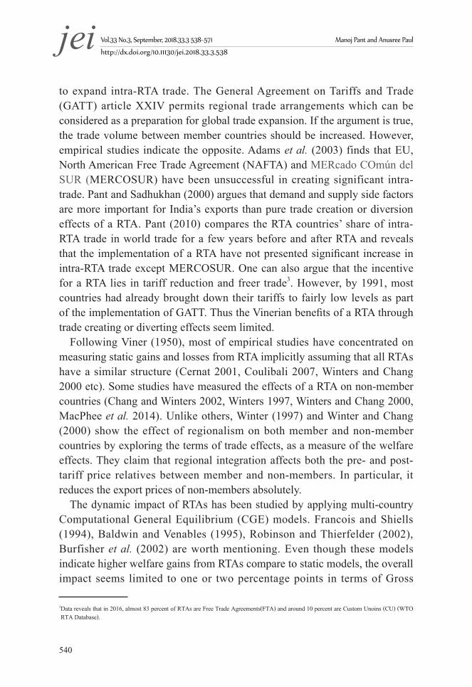
Next, the second stage problem can be written as:
������ = (∑ ���� )��� ������� �� ��� = ∑ �������� (6)
where ��� is the total nominal income of country j’s residents spent on x-goods.
The country j’s demand function for x-goods produced in country i can be obtained by solving the Equation (6):
To solve the consumer’s optimization problem, two-stage budgeting procedure is utilized. First, the consumer allocates her income between the homogeneous goods and basket of differentiated goods and then chooses differentiated products among the basket of differentiated goods.
We define the quantity and price indices as:
���� ≡ (∑ ���� )�
��,
����� ≡ min� �∑ �������:� (∑ ���� )��� = ��
(3)
The quantity index is the sub-utility function related to differentiated goods, while the price index is the minimum expenditure needed to buy one unit of composite differentiated commodity. Thus, the first stage maximization problem of country-j’s consumers can be written as:
��� ��∗ = (����)�(���)��� subject to �� = ��������� � �� ∑ ���� (4)
Solving the Equation (4) gives us the following import demand functions:
���� = ��������
� ��� = (� � �)����� = �� � � (5)
Next, the second stage problem can be written as:
������ = (∑ ���� )��� ������� �� ��� = ∑ �������� (6)
where ��� is the total nominal income of country j’s residents spent on x-goods.
The country j’s demand function for x-goods produced in country i can be obtained by solving the Equation (6):
The quantity index is the sub-utility function related to differentiated goods, while the price index is the minimum expenditure needed to buy one unit of composite differentiated commodity.
Thus, the first stage maximization problem of country-j’s consumers can be written as:
To solve the consumer’s optimization problem, two-stage budgeting procedure is utilized. First, the consumer allocates her income between the homogeneous goods and basket of differentiated goods and then chooses differentiated products among the basket of differentiated goods.
We define the quantity and price indices as:
���� ≡ (∑ ���� )�
��,
����� ≡ min� �∑ �������:� (∑ ���� )��� = ��
(3)
The quantity index is the sub-utility function related to differentiated goods, while the price index is the minimum expenditure needed to buy one unit of composite differentiated commodity. Thus, the first stage maximization problem of country-j’s consumers can be written as:
��� ��∗ = (����)�(���)��� subject to �� = ��������� � �� ∑ ���� (4)
Solving the Equation (4) gives us the following import demand functions:
���� = ��������
� ��� = (� � �)����� = �� � � (5)
Next, the second stage problem can be written as:
������ = (∑ ���� )��� ������� �� ��� = ∑ �������� (6)
where ��� is the total nominal income of country j’s residents spent on x-goods.
The country j’s demand function for x-goods produced in country i can be obtained by solving the Equation (6):
(4)
Solving the Equation (4) gives us the following import demand functions:
To solve the consumer’s optimization problem, two-stage budgeting procedure is utilized. First, the consumer allocates her income between the homogeneous goods and basket of differentiated goods and then chooses differentiated products among the basket of differentiated goods.
We define the quantity and price indices as:
���� ≡ (∑ ���� )�
��,
����� ≡ min� �∑ �������:� (∑ ���� )��� = ��
(3)
The quantity index is the sub-utility function related to differentiated goods, while the price index is the minimum expenditure needed to buy one unit of composite differentiated commodity. Thus, the first stage maximization problem of country-j’s consumers can be written as:
��� ��∗ = (����)�(���)��� subject to �� = ��������� � �� ∑ ���� (4)
Solving the Equation (4) gives us the following import demand functions:
���� = ��������
� ��� = (� � �)����� = �� � � (5)
Next, the second stage problem can be written as:
������ = (∑ ���� )��� ������� �� ��� = ∑ �������� (6)
where ��� is the total nominal income of country j’s residents spent on x-goods.
The country j’s demand function for x-goods produced in country i can be obtained by solving the Equation (6):
(5)
of trade costs (Anderson and Van Wincoop 2003).
Vol.33 No.3, September, 2018.33.3 538~571� Manoj Pant and Anusree Paul
http://dx.doi.org/10.11130/jei.2018.33.3.538jei
546
Next, the second stage problem can be written as:
To solve the consumer’s optimization problem, two-stage budgeting procedure is utilized. First, the consumer allocates her income between the homogeneous goods and basket of differentiated goods and then chooses differentiated products among the basket of differentiated goods.
We define the quantity and price indices as:
���� ≡ (∑ ���� )�
��,
����� ≡ min� �∑ �������:� (∑ ���� )��� = ��
(3)
The quantity index is the sub-utility function related to differentiated goods, while the price index is the minimum expenditure needed to buy one unit of composite differentiated commodity. Thus, the first stage maximization problem of country-j’s consumers can be written as:
��� ��∗ = (����)�(���)��� subject to �� = ��������� � �� ∑ ���� (4)
Solving the Equation (4) gives us the following import demand functions:
���� = ��������
� ��� = (� � �)����� = �� � � (5)
Next, the second stage problem can be written as:
������ = (∑ ���� )��� ������� �� ��� = ∑ �������� (6)
where ��� is the total nominal income of country j’s residents spent on x-goods.
The country j’s demand function for x-goods produced in country i can be obtained by solving the Equation (6):
(6)
where Mxj is the total nominal income of country j’s residents spent on x-goods.
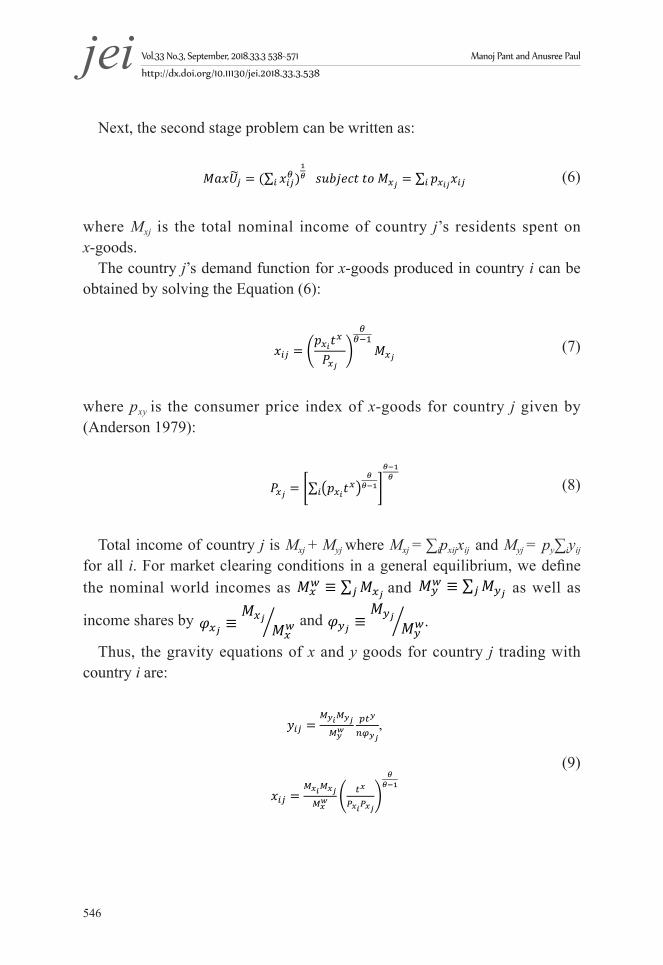
The country j’s demand function for x-goods produced in country i can be obtained by solving the Equation (6):
��� = ������
����
����
��� (7)
where ��� is the consumer price index of x-goods for country j given by(Anderson 1979):
��� = �∑ ��������
���� ����
�(8)
Total income of country j is ���+��� where ��� = ∑ �������� and ��� = �� ∑ ����
for all i. For market clearing conditions in a general equilibrium, we define the nominal world
incomes as ��� ≡ ∑ ���� and ��� ≡ ∑ ���� as well as income shares by ��� ≡ ������
�
and ��� ≡ ������
� .
Thus, the gravity equations of � and � goods for country j trading with country i are:
��� = ���������
����
�����, (9)
��� = ���������
� ��
�������
����
with ���
���� = �∑ ���
����������� �
���� ����
�and ��� ≡ ���
���
(10)
In general the model indicates implementation of two demand equations of inter- and intra- industry trade as shown in the Equations (9) and (10). However, since India has significant volume of both kinds of trade, we are implementing (9) and (10) together in a single gravity model equation.
(7)
where pxy is the consumer price index of x-goods for country j given by (Anderson 1979):
��� = ������
����
����
��� (7)
where ��� is the consumer price index of x-goods for country j given by(Anderson 1979):
��� = �∑ ��������
���� ����
�(8)
Total income of country j is ���+��� where ��� = ∑ �������� and ��� = �� ∑ ����
for all i. For market clearing conditions in a general equilibrium, we define the nominal world
incomes as ��� ≡ ∑ ���� and ��� ≡ ∑ ���� as well as income shares by ��� ≡ ������
�
and ��� ≡ ������
� .
Thus, the gravity equations of � and � goods for country j trading with country i are:
��� = ���������
����
�����, (9)
��� = ���������
� ��
�������
����
with ���
���� = �∑ ���
����������� �
���� ����
�and ��� ≡ ���
���
(10)
In general the model indicates implementation of two demand equations of inter- and intra- industry trade as shown in the Equations (9) and (10). However, since India has significant volume of both kinds of trade, we are implementing (9) and (10) together in a single gravity model equation.
(8)
Total income of country j is Mxj + Myj where Mxj = ∑ipxijxij and Myj = py∑iyij
for all i. For market clearing conditions in a general equilibrium, we define the nominal world incomes as
��� = ������
����
����
��� (7)
where ��� is the consumer price index of x-goods for country j given by(Anderson 1979):
��� = �∑ ��������
���� ����
�(8)
Total income of country j is ���+��� where ��� = ∑ �������� and ��� = �� ∑ ����
for all i. For market clearing conditions in a general equilibrium, we define the nominal world
incomes as ��� ≡ ∑ ���� and ��� ≡ ∑ ���� as well as income shares by ��� ≡ ������
�
and ��� ≡ ������
� .
Thus, the gravity equations of � and � goods for country j trading with country i are:
��� = ���������
����
�����, (9)
��� = ���������
� ��
�������
����
with ���
���� = �∑ ���
����������� �
���� ����
�and ��� ≡ ���
���
(10)
In general the model indicates implementation of two demand equations of inter- and intra- industry trade as shown in the Equations (9) and (10). However, since India has significant volume of both kinds of trade, we are implementing (9) and (10) together in a single gravity model equation.
and
��� = ������
����
����
��� (7)
where ��� is the consumer price index of x-goods for country j given by(Anderson 1979):
��� = �∑ ��������
���� ����
�(8)
Total income of country j is ���+��� where ��� = ∑ �������� and ��� = �� ∑ ����
for all i. For market clearing conditions in a general equilibrium, we define the nominal world
incomes as ��� ≡ ∑ ���� and ��� ≡ ∑ ���� as well as income shares by ��� ≡ ������
�
and ��� ≡ ������
� .
Thus, the gravity equations of � and � goods for country j trading with country i are:
��� = ���������
����
�����, (9)
��� = ���������
� ��
�������
����
with ���
���� = �∑ ���
����������� �
���� ����
�and ��� ≡ ���
���
(10)
In general the model indicates implementation of two demand equations of inter- and intra- industry trade as shown in the Equations (9) and (10). However, since India has significant volume of both kinds of trade, we are implementing (9) and (10) together in a single gravity model equation.
as well as
income shares by
��� = ������
����
����
��� (7)
where ��� is the consumer price index of x-goods for country j given by(Anderson 1979):
��� = �∑ ��������
���� ����
�(8)
Total income of country j is ���+��� where ��� = ∑ �������� and ��� = �� ∑ ����
for all i. For market clearing conditions in a general equilibrium, we define the nominal world
incomes as ��� ≡ ∑ ���� and ��� ≡ ∑ ���� as well as income shares by ��� ≡ ������
�
and ��� ≡ ������
� .
Thus, the gravity equations of � and � goods for country j trading with country i are:
��� = ���������
����
�����, (9)
��� = ���������
� ��
�������
����
with ���
���� = �∑ ���
����������� �
���� ����
�and ��� ≡ ���
���
(10)
In general the model indicates implementation of two demand equations of inter- and intra- industry trade as shown in the Equations (9) and (10). However, since India has significant volume of both kinds of trade, we are implementing (9) and (10) together in a single gravity model equation.
and
��� = ������
����
����
��� (7)
where ��� is the consumer price index of x-goods for country j given by(Anderson 1979):
��� = �∑ ��������
���� ����
�(8)
Total income of country j is ���+��� where ��� = ∑ �������� and ��� = �� ∑ ����
for all i. For market clearing conditions in a general equilibrium, we define the nominal world
incomes as ��� ≡ ∑ ���� and ��� ≡ ∑ ���� as well as income shares by ��� ≡ ������
�
and ��� ≡ ������
� .
Thus, the gravity equations of � and � goods for country j trading with country i are:
��� = ���������
����
�����, (9)
��� = ���������
� ��
�������
����
with ���
���� = �∑ ���
����������� �
���� ����
�and ��� ≡ ���
���
(10)
In general the model indicates implementation of two demand equations of inter- and intra- industry trade as shown in the Equations (9) and (10). However, since India has significant volume of both kinds of trade, we are implementing (9) and (10) together in a single gravity model equation.
Thus, the gravity equations of x and y goods for country j trading with country i are:
��� = ������
����
����
��� (7)
where ��� is the consumer price index of x-goods for country j given by(Anderson 1979):
��� = �∑ ��������
���� ����
�(8)
Total income of country j is ���+��� where ��� = ∑ �������� and ��� = �� ∑ ����
for all i. For market clearing conditions in a general equilibrium, we define the nominal world
incomes as ��� ≡ ∑ ���� and ��� ≡ ∑ ���� as well as income shares by ��� ≡ ������
�
and ��� ≡ ������
� .
Thus, the gravity equations of � and � goods for country j trading with country i are:
��� = ���������
���
����, (9)
��� = ���������
� ��
�������
����
with ���
���� = �∑ ���
����������� �
���� ����
�and ��� ≡ ���
���
(10)
In general the model indicates implementation of two demand equations of inter- and intra- industry trade as shown in the Equations (9) and (10). However, since India has significant volume of both kinds of trade, we are implementing (9) and (10) together in a single gravity model equation.
(9)
The Role of Regional Trade Agreements: in the Case of India jei
547
��� = ������
����
����
��� (7)
where ��� is the consumer price index of x-goods for country j given by(Anderson 1979):
��� = �∑ ��������
���� ����
�(8)
Total income of country j is ���+��� where ��� = ∑ �������� and ��� = �� ∑ ����
for all i. For market clearing conditions in a general equilibrium, we define the nominal world
incomes as ��� ≡ ∑ ���� and ��� ≡ ∑ ���� as well as income shares by ��� ≡ ������
�
and ��� ≡ ������
� .
Thus, the gravity equations of � and � goods for country j trading with country i are:
��� = ���������
����
�����, (9)
��� = ���������
� ��
�������
����
with ���
���� = �∑ ���
����������� �
���� ����
�and ��� ≡ ���
���
(10)
In general the model indicates implementation of two demand equations of inter- and intra- industry trade as shown in the Equations (9) and (10). However, since India has significant volume of both kinds of trade, we are implementing (9) and (10) together in a single gravity model equation.
(10)
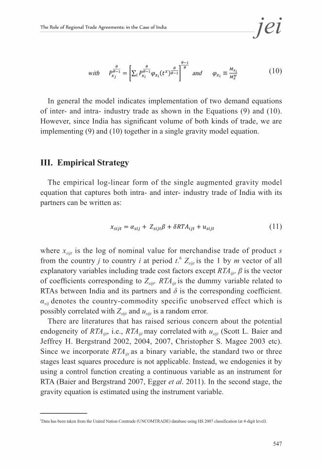
In general the model indicates implementation of two demand equations of inter- and intra- industry trade as shown in the Equations (9) and (10). However, since India has significant volume of both kinds of trade, we are implementing (9) and (10) together in a single gravity model equation.
III. Empirical Strategy
The empirical log-linear form of the single augmented gravity model equation that captures both intra- and inter- industry trade of India with its partners can be written as:
III. Empirical Strategy
The empirical log-linear form of the single augmented gravity model equation that captures both intra- and inter- industry trade of India with its partners can be written as:
(11)
where is the log of nominal value for merchandise trade of product s from the country j to
country i at period t.6 is the 1 by m vector of all explanatory variables including trade cost
factors except . is the vector of coefficients corresponding to is the
dummy variable related to RTAs between India and its partners and is the corresponding coefficient. denotes the country-commodity specific unobserved effect which is possibly
correlated with and is a random error.
There are literatures that has raised serious concern about the potential endogeneity of , i.e., may correlated with (Scott L. Baier and Jeffrey H. Bergstrand 2002,
2004, 2007, Christopher S. Magee 2003 etc). Since we incorporate as a binary variable,
the standard two or three stages least squares procedure is not applicable. Instead, we endogenies it by using a control function creating a continuous variable as an instrument for RTA (Baier and Bergstrand 2007, Egger et al. 2011). In the second stage, the gravity equation is estimated using the instrument variable.
A. Data
India’s top 25~30 partner countries, whose export and import share are at least one percent of India’s total trade at 4-digit level for each year (HS 2007 classification), are extracted. Data
6 Data has been taken from the United Nation Comtrade (UNCOMTRADE) database using HS 2007 classification (at 4-digit level).
(11)
where xsijt is the log of nominal value for merchandise trade of product s from the country j to country i at period t.6 Zsijt is the 1 by m vector of all explanatory variables including trade cost factors except RTAijt. β is the vector of coefficients corresponding to Zsijt. RTAijt is the dummy variable related to RTAs between India and its partners and δ is the corresponding coefficient. αsij denotes the country-commodity specific unobserved effect which is possibly correlated with Zsijt and usijt is a random error.
There are literatures that has raised serious concern about the potential endogeneity of RTAijt, i.e., RTAijt may correlated with usijt (Scott L. Baier and Jeffrey H. Bergstrand 2002, 2004, 2007, Christopher S. Magee 2003 etc). Since we incorporate RTAijt as a binary variable, the standard two or three stages least squares procedure is not applicable. Instead, we endogenies it by using a control function creating a continuous variable as an instrument for RTA (Baier and Bergstrand 2007, Egger et al. 2011). In the second stage, the gravity equation is estimated using the instrument variable.
6Data has been taken from the United Nation Comtrade (UNCOMTRADE) database using HS 2007 classification (at 4-digit level).
Vol.33 No.3, September, 2018.33.3 538~571� Manoj Pant and Anusree Paul
http://dx.doi.org/10.11130/jei.2018.33.3.538jei
548
A. Data
India’s top 25~30 partner countries, whose export and import share are at least one percent of India’s total trade at 4-digit level for each year (HS 2007 classification), are extracted. Data are collected from World Integrated Trade Solution (WITS) database. We also select top traded commodities at 4-digit level whose trade share is at least one percent of India’s total trade for each year. The number of commodities varies between 184~265 for the chosen years hence constructed panel is unbalanced with year and country by commodity dimension for the period of 2007~2015. The explanatory variables in Zsijt are as follows:
Market size proxies and trade cost variables: we take logs of India’s GDP (yjt) and its partner countries’ GDP (yit) as proxies for their respective market sizes. It is expected that bilateral trade between India and its partner is positively affected by size of their markets. Nominal GDP in US dollars and population data are collected from the World Bank World Develop Indicator (WBWDI). Missing data has been supplemented from the International Monetary Fund (IMF) World Economic Outlook (October 2015).
The direct measures of trade frictions tx and ty are not available. However, proxy variables which can account for the trade costs between the countries are available. Following the literatures, we assume that tx and ty are functions of time invariant observable bilateral log-distance between India and its partner (Dij)
7.The data are sourced from the Centre d’Etudes Prospectives et d’Informations Internationales (CEPII) database for gravity variables.
Regional trade agreement dummies: In the most of empirical literatures, trade policy variable has been considered as an element of trade costs. Following this convention, RTA between India and its trading partners are considered as an important indicator variable or element of tx and ty. We construct a dummy variable RTAijt
which takes the value one if India and its partner are member of the same trade bloc, and zero otherwise. Similarly, the trade diversion effect is captured by the dummy variable RTA_2ijt
which is equal to one if India and its partner are not members of the same trade bloc but of a different trade bloc, and zero otherwise. Data on trade agreements are obtained from the Design of Trade Agreements (DESTA).
7Weighted distance between India and its partner country.

The Role of Regional Trade Agreements: in the Case of India jei
549
Intra-industry trade dummy and relative factor endowments: We calculate the commodity-wise Grubel and Lloyd (GL) index to categorize the traded commodities into inter- and intra-industry trade. The GL index of product s traded between home country j and its partner i is given by
are collected from World Integrated Trade Solution (WITS) database. We also select top traded commodities at 4-digit level whose trade share is at least one percent of India’s total trade for each year. The number of commodities varies between 184~265 for the chosen years hence constructed panel is unbalanced with year and country by commodity dimension for the period of 2007~2015. The explanatory variables in ����� are as follows:
Market size proxies and trade cost variables: we take logs of India’s GDP (���) and its
partner countries’ GDP (���) as proxies for their respective market sizes. It is expected that bilateral trade between India and its partner is positively affected by size of their markets. Nominal GDP in US dollars and population data are collected from the World Bank World Develop Indicator (WBWDI). Missing data has been supplemented from the International Monetary Fund (IMF) World Economic Outlook (October 2015).
The direct measures of trade frictions �� and �� are not available. However, proxy variables which can account for the trade costs between the countries are available. Following the literatures, we assume that �� and �� are functions of time invariant observable bilateral
log-distance between India and its partner (���)7.The data are sourced from the Centre d'Etudes
Prospectives et d'Informations Internationales (CEPII) database for gravity variables. Regional trade agreement dummies: In the most of empirical literatures, trade policy
variable has been considered as an element of trade costs. Following this convention, RTA between India and its trading partners are considered as an important indicator variable or element of ��and ��. We construct a dummy variable ������ which takes the value one if
India and its partner are member of the same trade bloc, and zero otherwise. Similarly, the trade diversion effect is captured by the dummy variable �������� which is equal to one if India and
its partner are not members of the same trade bloc but of a different trade bloc, and zero otherwise. Data on trade agreements are obtained from the Design of Trade Agreements (DESTA).
Intra-industry trade dummy and relative factor endowments: We calculate the commodity-wise Grubel and Lloyd (GL) index to categorize the traded commodities into inter- and intra-industry trade. The GL index of product s traded between home country j and its partner i is
given by ������� = 1 − ������� ������� � ������� ������� ) for each period t. If the value of ������� is less or equal to 0.1,
the commodity s is considered as inter industry trade type and if the value is greater than 0.1, the
7 Weighted distance between India and its partner country.
for each period t. If the value of IITsijt is less or equal
to 0.1, the commodity s is considered as inter industry trade type and if the value is greater than 0.1, the commodity s is labelled as intra-industry trade type (Fontagné and Freudenberg 1997). IIT_dimsijt is equal to one if the trade type is intra-industry, zero otherwise.
Neo classical model of trade traces endowment differences as the driver of trade. We use the difference in per capita income of countries (DPCI) as a proxy for factor endowment differences, i.e., a log value of DPCI (dpciijt) is included as one of explanatory variables. Data are collected from the WBWDI. Missing data is supplemented from the IMF World Economic Outlook October 2015 Database.
B. Econometric model
The unobserved heterogeneity that arises from endogenous binary explanatory variables (EEV) can be handled through a two-step control function approach. We consider the traditional switching regression model and follow the methodology of Semykina and Wooldridge (2010) as well as Murtazashvili and Wooldridge (2016).
Let x1sijt be the log of bilateral trade flows between India and its partner i
with RTA and x0sijt be the bilateral trade flows between India and its partner i
without RTA at a time period t. Assume that x0sijt and x1
sijt have a standard form in a gravity equation:
commodity s is labelled as intra-industry trade type (Fontagné and Freudenberg 1997). ����������� is equal to one if the trade type is intra-industry, zero otherwise.
Neo classical model of trade traces endowment differences as the driver of trade. We use the difference in per capita income of countries (DPCI) as a proxy for factor endowment differences, i.e., a log value of DPCI (�������) is included as one of explanatory variables. Data
are collected from the WBWDI. Missing data is supplemented from the IMF World Economic Outlook October 2015 Database.
B. Econometric model
The unobserved heterogeneity that arises from endogenous binary explanatory variables (EEV) can be handled through a two-step control function approach. We consider the traditional switching regression model and follow the methodology of Semykina and Wooldridge (2010) as well as Murtazashvili and Wooldridge (2016).
Let � ����� be the log of bilateral trade flows between India and its partner i with RTA and
� ����� be the bilateral trade flows between India and its partner i without RTA at a time period t.
Assume that � ����� ��� � ����
� have a standard form in a gravity equation:
� ����� � ����� � ������� � ������ � ������� � ������ (12)
� ����� � ����� � ������� � ������ � ������� � ������ (13)
where ����� and ����� are the time invariant unobserved heterogeneity and ������ and ������are random errors of with and without RTA regime respectively. Time-constant and time-varying
unobservables are defined as ����� � ������ � ������ and ����� � ������ � ������.
In reality, one can only observe a trade flow in the presence or absence of a RTA, thus we define the observed outcome x as:
����� � ��������� ����� � �� � �������� ����
� (14)
(12)
commodity s is labelled as intra-industry trade type (Fontagné and Freudenberg 1997). ����������� is equal to one if the trade type is intra-industry, zero otherwise.
Neo classical model of trade traces endowment differences as the driver of trade. We use the difference in per capita income of countries (DPCI) as a proxy for factor endowment differences, i.e., a log value of DPCI (�������) is included as one of explanatory variables. Data
are collected from the WBWDI. Missing data is supplemented from the IMF World Economic Outlook October 2015 Database.
B. Econometric model
The unobserved heterogeneity that arises from endogenous binary explanatory variables (EEV) can be handled through a two-step control function approach. We consider the traditional switching regression model and follow the methodology of Semykina and Wooldridge (2010) as well as Murtazashvili and Wooldridge (2016).
Let � ����� be the log of bilateral trade flows between India and its partner i with RTA and
� ����� be the bilateral trade flows between India and its partner i without RTA at a time period t.
Assume that � ����� ��� � ����
� have a standard form in a gravity equation:
� ����� � ����� � ������� � ������ � ������� � ������ (12)
� ����� � ����� � ������� � ������ � ������� � ������ (13)
where ����� and ����� are the time invariant unobserved heterogeneity and ������ and ������are random errors of with and without RTA regime respectively. Time-constant and time-varying
unobservables are defined as ����� � ������ � ������ and ����� � ������ � ������.
In reality, one can only observe a trade flow in the presence or absence of a RTA, thus we define the observed outcome x as:
����� � ��������� ����� � �� � �������� ����
� (14)
(13)
where α0sij and α1
sij are the time invariant unobserved heterogeneity and u0sijt

Vol.33 No.3, September, 2018.33.3 538~571� Manoj Pant and Anusree Paul
http://dx.doi.org/10.11130/jei.2018.33.3.538jei
550
and u1sijt are random errors of with and without RTA regime respectively.
Time-constant and time-varying unobservables are defined as a0sij + u0
sijt = e0
sijt and α1sij + u1
sijt = e1sijt .
In reality, one can only observe a trade flow in the presence or absence of a RTA, thus we define the observed outcome x as:
commodity s is labelled as intra-industry trade type (Fontagné and Freudenberg 1997). ����������� is equal to one if the trade type is intra-industry, zero otherwise.
Neo classical model of trade traces endowment differences as the driver of trade. We use the difference in per capita income of countries (DPCI) as a proxy for factor endowment differences, i.e., a log value of DPCI (�������) is included as one of explanatory variables. Data
are collected from the WBWDI. Missing data is supplemented from the IMF World Economic Outlook October 2015 Database.
B. Econometric model
The unobserved heterogeneity that arises from endogenous binary explanatory variables (EEV) can be handled through a two-step control function approach. We consider the traditional switching regression model and follow the methodology of Semykina and Wooldridge (2010) as well as Murtazashvili and Wooldridge (2016).
Let � ����� be the log of bilateral trade flows between India and its partner i with RTA and
� ����� be the bilateral trade flows between India and its partner i without RTA at a time period t.
Assume that � ����� ��� � ����
� have a standard form in a gravity equation:
� ����� � ����� � ������� � ������ � ������� � ������ (12)
� ����� � ����� � ������� � ������ � ������� � ������ (13)
where ����� and ����� are the time invariant unobserved heterogeneity and ������ and ������are random errors of with and without RTA regime respectively. Time-constant and time-varying
unobservables are defined as ����� � ������ � ������ and ����� � ������ � ������.
In reality, one can only observe a trade flow in the presence or absence of a RTA, thus we define the observed outcome x as:
����� � ��������� ����� � �� � �������� ����
� (14)(14)
Substituting (12) and (13) in (14) gives:Substituting (12) and (13) in (14) gives:
����� = ����� + ������� + ������������� + ������ + ������������ (15)
where �� = �� � �� and ������ = ������ � ������.
ℎ����8 is a 1 by m vector9 of instruments which is strictly exogeneous conditional on ����,
i,e., ��������ℎ����� ����� � ��������ℎ���� ����� = � . This allows correlation between ���� and
ℎ���� . Wooldridge (1995) have used fixed effects to remove unobserved heterogeneity by
permitting arbitrary correlation between ���� and ℎ����.
An unobserved heterogeneity is assumed to be linearly related to ℎ���� (Mundlak 1978
assumption), which implies:
������ = ℎ������ + ������ and ������ = ℎ������ + ������ (16)
where ℎ���� = ��� ∑ ℎ�������� and ������� ������ are independent of ℎ���� . These assumptions
impose strict exogeneity of ℎ���� with respect to ������ ��� ������.
Substituting (16) into (15), we get:
����� = ������� + ������������� + ℎ������ + ������ℎ������� ������ � ������������
(17)
Following Murtazashvili and Wooldridge (2016), we specify the Mundlak version of binary response correlated random effect model for ������ is defined as:
������ = ���� + ℎ����� + ℎ����� + ���� � �� � = �� � � � � � (18)
8 The vector ℎ���� comprises all set of variables affecting India’s participation decision in a regional trade agreement with its partner country. It contains elements of ����� along with the set of instrumental variables that are excluded from (16). 9 With m>n, to satisfy the identification condition, where, ����� is the (1x m) vector and ℎ���� is the (1x n) vector.
(15)
where γ1 = β1- β0 and v1sijt = e1
sijt - e0
sijt.hsijt
8 is a 1 by m vector9 of instruments which is strictly exogeneous conditional on αsij, i,e., E(usijt│hsijt,αsij)≡E(usijt│hsij,αsij)=0. This allows correlation between αsij and hsijt. Wooldridge (1995) have used fixed effects to remove unobserved heterogeneity by permitting arbitrary correlation between αsij and hsijt.
An unobserved heterogeneity is assumed to be linearly related to hsij (Mundlak 1978 assumption), which implies:
Substituting (12) and (13) in (14) gives:
����� = ����� + ������� + ������������� + ������ + ������������ (15)
where �� = �� � �� and ������ = ������ � ������.
ℎ����8 is a 1 by m vector9 of instruments which is strictly exogeneous conditional on ����,
i,e., ��������ℎ����� ����� � ��������ℎ���� ����� = � . This allows correlation between ���� and
ℎ���� . Wooldridge (1995) have used fixed effects to remove unobserved heterogeneity by
permitting arbitrary correlation between ���� and ℎ����.
An unobserved heterogeneity is assumed to be linearly related to ℎ���� (Mundlak 1978
assumption), which implies:
������ = ℎ������ + ������ and ������ = ℎ������ + ������ (16)
where ℎ���� = ��� ∑ ℎ�������� and ������� ������ are independent of ℎ���� . These assumptions
impose strict exogeneity of ℎ���� with respect to ������ ��� ������.
Substituting (16) into (15), we get:
����� = ������� + ������������� + ℎ������ + ������ℎ������� ������ � ������������
(17)
Following Murtazashvili and Wooldridge (2016), we specify the Mundlak version of binary response correlated random effect model for ������ is defined as:
������ = ���� + ℎ����� + ℎ����� + ���� � �� � = �� � � � � � (18)
8 The vector ℎ���� comprises all set of variables affecting India’s participation decision in a regional trade agreement with its partner country. It contains elements of ����� along with the set of instrumental variables that are excluded from (16). 9 With m>n, to satisfy the identification condition, where, ����� is the (1x m) vector and ℎ���� is the (1x n) vector.
(16)
where h sij = T -1
Substituting (12) and (13) in (14) gives:
����� = ����� + ������� + ������������ �� + ������ + ������������ (15)
where �� = �� � �� and ������ = ������ � ������.
ℎ����8 is a 1 by m vector9 of instruments which is strictly exogeneous conditional on ����,
i,e., ��������ℎ����� ����� � ��������ℎ���� ����� = � . This allows correlation between ���� and
ℎ���� . Wooldridge (1995) have used fixed effects to remove unobserved heterogeneity by
permitting arbitrary correlation between ���� and ℎ����.
An unobserved heterogeneity is assumed to be linearly related to ℎ���� (Mundlak 1978
assumption), which implies:
������ = ℎ������ + ������ and ������ = ℎ������ + ������ (16)
where ℎ���� = ��� ∑ ℎ�������� and ������� ������ are independent of ℎ���� . These assumptions
impose strict exogeneity of ℎ���� with respect to ������ ��� ������.
Substituting (16) into (15), we get:
����� = ������� + ������������� + ℎ������ + ������ℎ������� ������ � ������������
(17)
Following Murtazashvili and Wooldridge (2016), we specify the Mundlak version of binary response correlated random effect model for ������ is defined as:
������ = ���� + ℎ����� + ℎ����� + ���� � �� � = �� � � � � � (18)
8 The vector ℎ���� comprises all set of variables affecting India’s participation decision in a regional trade agreement with its partner country. It contains elements of ����� along with the set of instrumental variables that are excluded from (16). 9 With m>n, to satisfy the identification condition, where, ����� is the (1x m) vector and ℎ���� is the (1x n) vector.
hsijt and r0sijt, r1
sijt are independent of hsijt. These assumptions impose strict exogeneity of hsijt with respect to u0
sijt and u1sijt.
Substituting (16) into (15), we get:
Substituting (12) and (13) in (14) gives:
����� = ����� + ������� + ������������ �� + ������ + ������������ (15)
where �� = �� � �� and ������ = ������ � ������.
ℎ����8 is a 1 by m vector9 of instruments which is strictly exogeneous conditional on ����,
i,e., ��������ℎ����� ����� � ��������ℎ���� ����� = � . This allows correlation between ���� and
ℎ���� . Wooldridge (1995) have used fixed effects to remove unobserved heterogeneity by
permitting arbitrary correlation between ���� and ℎ����.
An unobserved heterogeneity is assumed to be linearly related to ℎ���� (Mundlak 1978
assumption), which implies:
������ = ℎ������ + ������ and ������ = ℎ������ + ������ (16)
where ℎ���� = ��� ∑ ℎ�������� and ������� ������ are independent of ℎ���� . These assumptions
impose strict exogeneity of ℎ���� with respect to ������ ��� ������.
Substituting (16) into (15), we get:
����� = ������� + ������������� + ℎ������ + ������ℎ������� ������ � ������������
(17)
Following Murtazashvili and Wooldridge (2016), we specify the Mundlak version of binary response correlated random effect model for ������ is defined as:
������ = ���� + ℎ����� + ℎ����� + ���� � �� � = �� � � � � � (18)
8 The vector ℎ���� comprises all set of variables affecting India’s participation decision in a regional trade agreement with its partner country. It contains elements of ����� along with the set of instrumental variables that are excluded from (16). 9 With m>n, to satisfy the identification condition, where, ����� is the (1x m) vector and ℎ���� is the (1x n) vector.
(17)
8 The vector hsijt comprises all set of variables affecting India’s participation decision in a regional trade agreement with its partner country. It contains elements of Zsijt along with the set of instrumental variables that are excluded from (16).
9With m>n, to satisfy the identification condition, where, Zsijt is the (1x m) vector and hsijt is the (1x n) vector.
The Role of Regional Trade Agreements: in the Case of India jei
551
Following Murtazashvili and Wooldridge (2016), we specify the Mundlak version of binary response correlated random effect model for RTAijt is defined as:
Substituting (12) and (13) in (14) gives:
����� = ����� + ������� + ������������ �� + ������ + ������������ (15)
where �� = �� � �� and ������ = ������ � ������.
ℎ����8 is a 1 by m vector9 of instruments which is strictly exogeneous conditional on ����,
i,e., ��������ℎ����� ����� � ��������ℎ���� ����� = � . This allows correlation between ���� and
ℎ���� . Wooldridge (1995) have used fixed effects to remove unobserved heterogeneity by
permitting arbitrary correlation between ���� and ℎ����.
An unobserved heterogeneity is assumed to be linearly related to ℎ���� (Mundlak 1978
assumption), which implies:
������ = ℎ������ + ������ and ������ = ℎ������ + ������ (16)
where ℎ���� = ��� ∑ ℎ�������� and ������� ������ are independent of ℎ���� . These assumptions
impose strict exogeneity of ℎ���� with respect to ������ ��� ������.
Substituting (16) into (15), we get:
����� = ������� + ������������� + ℎ������ + ������ℎ������� ������ � ������������
(17)
Following Murtazashvili and Wooldridge (2016), we specify the Mundlak version of binary response correlated random effect model for ������ is defined as:
������ = ���� + ℎ����� + ℎ����� + ���� � �� � = �� � � � � � (18)
8 The vector ℎ���� comprises all set of variables affecting India’s participation decision in a regional trade agreement with its partner country. It contains elements of ����� along with the set of instrumental variables that are excluded from (16). 9 With m>n, to satisfy the identification condition, where, ����� is the (1x m) vector and ℎ���� is the (1x n) vector.
(18)
γt is the time specific intercept and ϵijt is an idiosyncratic error. The potential instrumental variables in hsijt is explained below. It is assumed that ϵijt ~ N(0,1) and r0
sijt, r1
sijt, єijt are independent of hsij.Under these assumptions we can write:
�� is the time specific intercept and ���� is an idiosyncratic error. The potential instrumental
variables in ℎ���� is explained below. It is assumed that ������(�,�) and ������, ������, ����are independent of ℎ���.
Under these assumptions we can write:
�(�����������, ℎ���) = �(�������� + ℎ����� + ℎ�����) (19)
where �(. ) is the generalised error function which is:
���������� + ℎ����� + ℎ������ = �������� �� + ℎ����� + ℎ������−� � − ��������� −�� − ℎ����� − ℎ������
(20)
where λ(. ) = �(.)�(.) is the inverse mills ratio, �(. ) is the standard normal density function and
�(. ) is the standard normal cumulative distribution function.
If we assume �(������������ = ������ and �(��
���������� = ������������ then one can
have �(������ + �������������������, ℎ���� = ���(. ) + ���������(. ).
Estimable gravity equation after accounting for the endogeneity of ������ is:
����� = ������� + ������������� + ℎ������ + ������ℎ������ + ���(. )
+���������(. ) + �����(21)
with ��������������, ℎ���� = �Standard two-step procedure is utilized to estimate the Equation (20), which produces
consistent and asymptotically normal estimators of ��, ��, ��, ��, �� and ��. In the first step,
probit of ������ on a full set of time period indicators ℎ���� and ℎ���� is estimated to get ���, ��and �� to obtain the generalised residuals as:
��(. ) = ������λ���� + ℎ������ + ℎ������� − �� − ������� λ�−��� − ℎ������ − ℎ������� (22)
(19)
where g(.) is the generalised error function which is:
�� is the time specific intercept and ���� is an idiosyncratic error. The potential instrumental
variables in ℎ���� is explained below. It is assumed that ������(�,�) and ������, ������, ����are independent of ℎ���.
Under these assumptions we can write:
�(�����������, ℎ���) = �(�������� + ℎ����� + ℎ�����) (19)
where �(. ) is the generalised error function which is:
���������� + ℎ����� + ℎ������ = �������� �� + ℎ����� + ℎ������−� � − ��������� −�� − ℎ����� − ℎ������
(20)
where λ(. ) = �(.)�(.) is the inverse mills ratio, �(. ) is the standard normal density function and
�(. ) is the standard normal cumulative distribution function.
If we assume �(������������ = ������ and �(��
���������� = ������������ then one can
have �(������ + �������������������, ℎ���� = ���(. ) + ���������(. ).
Estimable gravity equation after accounting for the endogeneity of ������ is:
����� = ������� + ������������� + ℎ������ + ������ℎ������ + ���(. )
+���������(. ) + �����(21)
with ��������������, ℎ���� = �Standard two-step procedure is utilized to estimate the Equation (20), which produces
consistent and asymptotically normal estimators of ��, ��, ��, ��, �� and ��. In the first step,
probit of ������ on a full set of time period indicators ℎ���� and ℎ���� is estimated to get ���, ��and �� to obtain the generalised residuals as:
��(. ) = ������λ���� + ℎ������ + ℎ������� − �� − ������� λ�−��� − ℎ������ − ℎ������� (22)
(20)
where
�� is the time specific intercept and ���� is an idiosyncratic error. The potential instrumental
variables in ℎ���� is explained below. It is assumed that ������(�,�) and ������, ������, ����are independent of ℎ���.
Under these assumptions we can write:
�(�����������, ℎ���) = �(�������� + ℎ����� + ℎ�����) (19)
where �(. ) is the generalised error function which is:
���������� + ℎ����� + ℎ������ = �������� �� + ℎ����� + ℎ������−� � − ��������� −�� − ℎ����� − ℎ������
(20)
where λ(. ) = �(.)�(.) is the inverse mills ratio, �(. ) is the standard normal density function and
�(. ) is the standard normal cumulative distribution function.
If we assume �(������������ = ������ and �(��
���������� = ������������ then one can
have �(������ + �������������������, ℎ���� = ���(. ) + ���������(. ).
Estimable gravity equation after accounting for the endogeneity of ������ is:
����� = ������� + ������������� + ℎ������ + ������ℎ������ + ���(. )
+���������(. ) + �����(21)
with ��������������, ℎ���� = �Standard two-step procedure is utilized to estimate the Equation (20), which produces
consistent and asymptotically normal estimators of ��, ��, ��, ��, �� and ��. In the first step,
probit of ������ on a full set of time period indicators ℎ���� and ℎ���� is estimated to get ���, ��and �� to obtain the generalised residuals as:
��(. ) = ������λ���� + ℎ������ + ℎ������� − �� − ������� λ�−��� − ℎ������ − ℎ������� (22)
is the inverse mills ratio,
�� is the time specific intercept and ���� is an idiosyncratic error. The potential instrumental
variables in ℎ���� is explained below. It is assumed that ������(�,�) and ������, ������, ����are independent of ℎ���.
Under these assumptions we can write:
�(�����������, ℎ���) = �(�������� + ℎ����� + ℎ�����) (19)
where �(. ) is the generalised error function which is:
���������� + ℎ����� + ℎ������ = �������� �� + ℎ����� + ℎ������−� � − ��������� −�� − ℎ����� − ℎ������
(20)
where λ(. ) = �(.)�(.) is the inverse mills ratio, �(. ) is the standard normal density function and
�(. ) is the standard normal cumulative distribution function.
If we assume �(������������ = ������ and �(��
���������� = ������������ then one can
have �(������ + �������������������, ℎ���� = ���(. ) + ���������(. ).
Estimable gravity equation after accounting for the endogeneity of ������ is:
����� = ������� + ������������� + ℎ������ + ������ℎ������ + ���(. )
+���������(. ) + �����(21)
with ��������������, ℎ���� = �Standard two-step procedure is utilized to estimate the Equation (20), which produces
consistent and asymptotically normal estimators of ��, ��, ��, ��, �� and ��. In the first step,
probit of ������ on a full set of time period indicators ℎ���� and ℎ���� is estimated to get ���, ��and �� to obtain the generalised residuals as:
��(. ) = ������λ���� + ℎ������ + ℎ������� − �� − ������� λ�−��� − ℎ������ − ℎ������� (22)
(.) is the standard normal density
function and
�� is the time specific intercept and ���� is an idiosyncratic error. The potential instrumental
variables in ℎ���� is explained below. It is assumed that ������(�,�) and ������, ������, ����are independent of ℎ���.
Under these assumptions we can write:
�(�����������, ℎ���) = �(�������� + ℎ����� + ℎ�����) (19)
where �(. ) is the generalised error function which is:
���������� + ℎ����� + ℎ������ = �������� �� + ℎ����� + ℎ������−� � − ��������� −�� − ℎ����� − ℎ������
(20)
where λ(. ) = �(.)�(.) is the inverse mills ratio, �(. ) is the standard normal density function and
�(. ) is the standard normal cumulative distribution function.
If we assume �(������������ = ������ and �(��
���������� = ������������ then one can
have �(������ + �������������������, ℎ���� = ���(. ) + ���������(. ).
Estimable gravity equation after accounting for the endogeneity of ������ is:
����� = ������� + ������������� + ℎ������ + ������ℎ������ + ���(. )
+���������(. ) + �����(21)
with ��������������, ℎ���� = �Standard two-step procedure is utilized to estimate the Equation (20), which produces
consistent and asymptotically normal estimators of ��, ��, ��, ��, �� and ��. In the first step,
probit of ������ on a full set of time period indicators ℎ���� and ℎ���� is estimated to get ���, ��and �� to obtain the generalised residuals as:
��(. ) = ������λ���� + ℎ������ + ℎ������� − �� − ������� λ�−��� − ℎ������ − ℎ������� (22)
(.) is the standard normal cumulative distribution function.If we assume E(r0
sijt|ϵijt) = μ0єijt and E(v1sijt|ϵijt) = μ1RTAijtϵijt then one can have
E(r0sijt + RTAijtv
1sijt|RTAijt, hsij) = μ0g(.) + μ1RTAijtg(.).
Estimable gravity equation after accounting for the endogeneity of RTAijt is:
(21)
�� is the time specific intercept and ���� is an idiosyncratic error. The potential instrumental
variables in ℎ���� is explained below. It is assumed that ������(�,�) and ������, ������, ����are independent of ℎ���.
Under these assumptions we can write:
�(�����������, ℎ���) = �(�������� + ℎ����� + ℎ�����) (19)
where �(. ) is the generalised error function which is:
���������� + ℎ����� + ℎ������ = �������� �� + ℎ����� + ℎ������−� � − ��������� −�� − ℎ����� − ℎ������
(20)
where λ(. ) = �(.)�(.) is the inverse mills ratio, �(. ) is the standard normal density function and
�(. ) is the standard normal cumulative distribution function.
If we assume �(������������ = ������ and �(��
���������� = ������������ then one can
have �(������ + �������������������, ℎ���� = ���(. ) + ���������(. ).
Estimable gravity equation after accounting for the endogeneity of ������ is:
����� = ������� + ������������� + ℎ������ + ������ℎ������ + ���(. )
+���������(. ) + �����(21)
with ��������������, ℎ���� = �Standard two-step procedure is utilized to estimate the Equation (20), which produces
consistent and asymptotically normal estimators of ��, ��, ��, ��, �� and ��. In the first step,
probit of ������ on a full set of time period indicators ℎ���� and ℎ���� is estimated to get ���, ��and �� to obtain the generalised residuals as:
��(. ) = ������λ���� + ℎ������ + ℎ������� − �� − ������� λ�−��� − ℎ������ − ℎ������� (22)
with E(ωsijt│RTAijt, hsij) = 0Standard two-step procedure is utilized to estimate the Equation (20),
which produces consistent and asymptotically normal estimators of β0, γ1, ρ0, ρ1, μ0 and μ1. In the first step, probit of RTAijt on a full set of time period indicators hsijt and hsij is estimated to get
�� is the time specific intercept and ���� is an idiosyncratic error. The potential instrumental
variables in ℎ���� is explained below. It is assumed that ������(�,�) and ������, ������, ����are independent of ℎ���.
Under these assumptions we can write:
�(�����������, ℎ���) = �(�������� + ℎ����� + ℎ�����) (19)
where �(. ) is the generalised error function which is:
���������� + ℎ����� + ℎ������ = �������� �� + ℎ����� + ℎ������−� � − ��������� −�� − ℎ����� − ℎ������
(20)
where λ(. ) = �(.)�(.) is the inverse mills ratio, �(. ) is the standard normal density function and
�(. ) is the standard normal cumulative distribution function.
If we assume �(������������ = ������ and �(��
���������� = ������������ then one can
have �(������ + �������������������, ℎ���� = ���(. ) + ���������(. ).
Estimable gravity equation after accounting for the endogeneity of ������ is:
����� = ������� + ������������� + ℎ������ + ������ℎ������ + ���(. )
+���������(. ) + �����(21)
with ��������������, ℎ���� = �Standard two-step procedure is utilized to estimate the Equation (20), which produces
consistent and asymptotically normal estimators of ��, ��, ��, ��, �� and ��. In the first step,
probit of ������ on a full set of time period indicators ℎ���� and ℎ���� is estimated to get ���, ��and �� to obtain the generalised residuals as:
��(. ) = ������λ���� + ℎ������ + ℎ������� − �� − ������� λ�−��� − ℎ������ − ℎ������� (22)
t, â and
�� is the time specific intercept and ���� is an idiosyncratic error. The potential instrumental
variables in ℎ���� is explained below. It is assumed that ������(�,�) and ������, ������, ����are independent of ℎ���.
Under these assumptions we can write:
�(�����������, ℎ���) = �(�������� + ℎ����� + ℎ�����) (19)
where �(. ) is the generalised error function which is:
���������� + ℎ����� + ℎ������ = �������� �� + ℎ����� + ℎ������−� � − ��������� −�� − ℎ����� − ℎ������
(20)
where λ(. ) = �(.)�(.) is the inverse mills ratio, �(. ) is the standard normal density function and
�(. ) is the standard normal cumulative distribution function.
If we assume �(������������ = ������ and �(��
���������� = ������������ then one can
have �(������ + �������������������, ℎ���� = ���(. ) + ���������(. ).
Estimable gravity equation after accounting for the endogeneity of ������ is:
����� = ������� + ������������� + ℎ������ + ������ℎ������ + ���(. )
+���������(. ) + �����(21)
with ��������������, ℎ���� = �Standard two-step procedure is utilized to estimate the Equation (20), which produces
consistent and asymptotically normal estimators of ��, ��, ��, ��, �� and ��. In the first step,
probit of ������ on a full set of time period indicators ℎ���� and ℎ���� is estimated to get ���, ��and �� to obtain the generalised residuals as:
��(. ) = ������λ���� + ℎ������ + ℎ������� − �� − ������� λ�−��� − ℎ������ − ℎ������� (22)
to obtain the generalised residuals as:
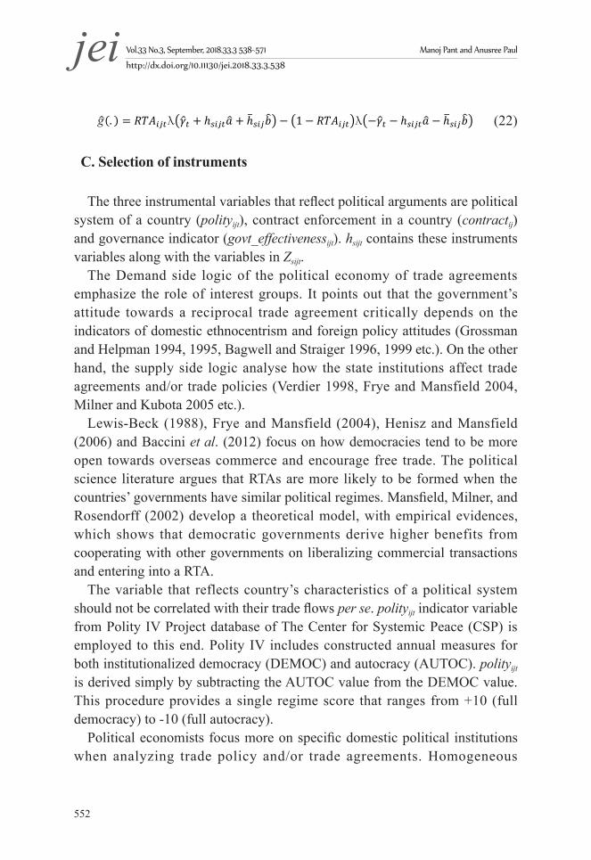
Vol.33 No.3, September, 2018.33.3 538~571� Manoj Pant and Anusree Paul
http://dx.doi.org/10.11130/jei.2018.33.3.538jei
552
�� is the time specific intercept and ���� is an idiosyncratic error. The potential instrumental
variables in ℎ���� is explained below. It is assumed that ������(�,�) and ������, ������, ����are independent of ℎ���.
Under these assumptions we can write:
�(�����������, ℎ���) = �(�������� + ℎ����� + ℎ�����) (19)
where �(. ) is the generalised error function which is:
���������� + ℎ����� + ℎ������ = �������� �� + ℎ����� + ℎ������−� � − ��������� −�� − ℎ����� − ℎ������
(20)
where λ(. ) = �(.)�(.) is the inverse mills ratio, �(. ) is the standard normal density function and
�(. ) is the standard normal cumulative distribution function.
If we assume �(������������ = ������ and �(��
���������� = ������������ then one can
have �(������ + �������������������, ℎ���� = ���(. ) + ���������(. ).
Estimable gravity equation after accounting for the endogeneity of ������ is:
����� = ������� + ������������� + ℎ������ + ������ℎ������ + ���(. )
+���������(. ) + �����(21)
with ��������������, ℎ���� = �Standard two-step procedure is utilized to estimate the Equation (20), which produces
consistent and asymptotically normal estimators of ��, ��, ��, ��, �� and ��. In the first step,
probit of ������ on a full set of time period indicators ℎ���� and ℎ���� is estimated to get ���, ��and �� to obtain the generalised residuals as:
��(. ) = ������λ���� + ℎ������ + ℎ������� − �� − �������λ�−��� − ℎ������ − ℎ������� (22)
�� is the time specific intercept and ���� is an idiosyncratic error. The potential instrumental
variables in ℎ���� is explained below. It is assumed that ������(�,�) and ������, ������, ����are independent of ℎ���.
Under these assumptions we can write:
�(�����������, ℎ���) = �(�������� + ℎ����� + ℎ�����) (19)
where �(. ) is the generalised error function which is:
���������� + ℎ����� + ℎ������ = �������� �� + ℎ����� + ℎ������−� � − ��������� −�� − ℎ����� − ℎ������
(20)
where λ(. ) = �(.)�(.) is the inverse mills ratio, �(. ) is the standard normal density function and
�(. ) is the standard normal cumulative distribution function.
If we assume �(������������ = ������ and �(��
���������� = ������������ then one can
have �(������ + �������������������, ℎ���� = ���(. ) + ���������(. ).
Estimable gravity equation after accounting for the endogeneity of ������ is:
����� = ������� + ������������� + ℎ������ + ������ℎ������ + ���(. )
+���������(. ) + �����(21)
with ��������������, ℎ���� = �Standard two-step procedure is utilized to estimate the Equation (20), which produces
consistent and asymptotically normal estimators of ��, ��, ��, ��, �� and ��. In the first step,
probit of ������ on a full set of time period indicators ℎ���� and ℎ���� is estimated to get ���, ��and �� to obtain the generalised residuals as:
��(. ) = ������λ���� + ℎ������ + ℎ������� − �� − �������λ�−��� − ℎ������ − ℎ������� (22)(22)
C. Selection of instruments
The three instrumental variables that reflect political arguments are political system of a country (polityijt), contract enforcement in a country (contractij) and governance indicator (govt_effectivenessijt). hsijt contains these instruments variables along with the variables in Zsijt.
The Demand side logic of the political economy of trade agreements emphasize the role of interest groups. It points out that the government’s attitude towards a reciprocal trade agreement critically depends on the indicators of domestic ethnocentrism and foreign policy attitudes (Grossman and Helpman 1994, 1995, Bagwell and Straiger 1996, 1999 etc.). On the other hand, the supply side logic analyse how the state institutions affect trade agreements and/or trade policies (Verdier 1998, Frye and Mansfield 2004, Milner and Kubota 2005 etc.).
Lewis-Beck (1988), Frye and Mansfield (2004), Henisz and Mansfield (2006) and Baccini et al. (2012) focus on how democracies tend to be more open towards overseas commerce and encourage free trade. The political science literature argues that RTAs are more likely to be formed when the countries’ governments have similar political regimes. Mansfield, Milner, and Rosendorff (2002) develop a theoretical model, with empirical evidences, which shows that democratic governments derive higher benefits from cooperating with other governments on liberalizing commercial transactions and entering into a RTA.
The variable that reflects country’s characteristics of a political system should not be correlated with their trade flows per se. polityijt indicator variable from Polity IV Project database of The Center for Systemic Peace (CSP) is employed to this end. Polity IV includes constructed annual measures for both institutionalized democracy (DEMOC) and autocracy (AUTOC). polityijt is derived simply by subtracting the AUTOC value from the DEMOC value. This procedure provides a single regime score that ranges from +10 (full democracy) to -10 (full autocracy).
Political economists focus more on specific domestic political institutions when analyzing trade policy and/or trade agreements. Homogeneous

The Role of Regional Trade Agreements: in the Case of India jei
553
institutional governance can enhance bilateral trust as well as bilateral trade (Anderson and Marcouiller 2002). Also the cost of adjustment generated by each other’s institutional environment would reduce (Beugelsdijk and Van Schaik 2001). The World Governance Indicator (WGI), government effectiveness10, can be a proxy for this and govt_effectivenessijt is derived as the absolute difference in the score variable, measuring the government effectiveness for an exporter and an importer. Data is collected from WGI data of World Bank.
Data for contract enforcement in a country (contractijt) are collected from the World Bank’s Doing Business database. The enforcing contracts indicator measures the time and cost for resolving a commercial dispute through a local first-instance court. It also measures the quality of judicial processes. When the two countries are close in terms of their contract enforcement, the probability of signing a bilateral trade agreement is higher. We take the absolute difference in the score variable, measuring the distance from the frontier of the contract-enforcement for India and its partner.
IV. Results
Two specifications of the gravity model are estimated. In first specification, the Equation (11) is estimated as shown in columns (1) to (3) of Table 1. The interactive dummy variables, dpciijt and IIT_dumsijt are incorporated to gauge the varying effect of factor endowment difference in intra-industry trade. IIT_dumsijt in the second specification is excluded since its correlation with interactive term is very high (0.98). The results are given in Table 1.
Columns (1) ~ (3) are the results of baseline model explained in (16) with various fixed effects. In columns (1), country-commodity (sij) fixed effects are considered along with time dummies. In columns (2), we take exporter-commodity (si) and importer-commodity (sj) dummies separately. Exporter (i), importer (j) and commodity (s) fixed effects are also considered separately in column (3). In columns (4) to (6), additional interactive term, dpciijt IIT_dumsijt, is incorporated and the fixed effects specifications are similar to
10 It captures the perceptions of the quality of public services, the quality of the civil service and the degree of its independence from political pressures, the quality of policy formulation and implementation, and the credibility of the government’s commitment to such policies.
(https://www.brookings.edu/wp-content/uploads/2016/06/09_wgi_kaufmann.pdf, page 4).

Vol.33 No.3, September, 2018.33.3 538~571� Manoj Pant and Anusree Paul
http://dx.doi.org/10.11130/jei.2018.33.3.538jei
554
regressions (1) to (3) respectively.The coefficients RTAijt of are found to be statistically significant at 1 percent
level in all specifications. is ranged between 0.14 and 0.19 which indicates RTAs increase India’s merchandise trade by 14.6 to 21 percent11. With regard to this results, previous studies for India are very limited in number and reveal mixed results when RTAs are considered as exogeneous variable. Moreover, most of the existing studies have analysed specific RTA’s impact on India’s trade. For example, Srinivasan and Archana (2009) shows counterproductive impact of major trade agreements on India’s trade flow during the period of 1981 to 2006. Few agreements such as India Sri Lanka Free trade Agreement (ISLFA) have generated trade creation effect on members and non-members as shown by Joshi (2012). Asia-Pacific Trade Agreement (APTA) is found to be an export creating trade agreement for India (Sen et al. 2015) whereas SAARC Preferential Trading Arrangement (SAPTA) has a negative impact on India, Pakistan and Sri Lanka’s trade (Akhter and Ghani 2010).
In all specifications, market size are found to be significant at the 1 percent significance level, which implies that it is a relevant determinant of India’s merchandise trade. In the specifications (2) and (5) we find that the distance between India and its partner, RTA_2ijt, captures the trade diversion or the trade creation effects when India’s partners are having any RTA with third countries. The coefficient is negative, which indicates India’s trade diversion effect. But this is found to be weakly significant or insignificant after controlling for the country and commodity level heterogeneity.
The positive coefficients of IIT_dumsijt indicate that India’s intra-industry trade over inter-industry trade is increased significantly by 33.6 percent to all types of countries when we control for time invariant heterogeneities as per specifications (1) and (2). But with those specifications, as shown in regressions (4) and (5), we find insignificant effect of factor endowment difference on intra-industry trade type.
11 When lnX is the dependent variable in a model and the coefficient of a dummy variable suggest a proportionate change in X, the exact percentage difference can be obtained through the semi elasticity calculation. Generally, if β1 is the coefficient of the dummy variable, say dum1, the exact percentage difference in the predicted X, when dum1 = 1 versus when dum1 = 0 is 100.[exp( 1)-1] (Wooldridge (2002):218).

The Role of Regional Trade Agreements: in the Case of India jei
555
Table 1. Results for the augmented gravity model
VariablesLog of nominal bilateral trade flow: In(Xsijt+1)
(1) (2) (3) (4) (5) (6)RTAijt(dummy variable)
0.14***
(0.04)0.16***
(0.04)0.19***
(0.05)0.14***
(0.04)0.16***
(0.05)0.19***
(0.05)Log of partner’s GDP (yit )
0.68***
(0.09)0.77***
(0.09)0.75***
(0.12)0.68***
(0.09)0.77***
(0.11)0.74***
(0.12)Log of India’s GDP (yit )
0.58***
(0.08)0.39***
(0.07)0.33***
(0.11)0.57***
(0.08)0.39***
(0.09)0.33***
(0.11)Log of distance (dit )
-1.04***
(0.23)-1.03***
(0.33) RTA_2ijt(dummy variable)
-0.07*
(0.04)-0.04(0.04)
-0.01(0.05)
-0.07*
(0.04)-0.04(0.05)
-0.01(0.05)
IIT_dimijt(dummy variable)
0.29***
(0.03)0.29***
(0.03)-0.03(0.05)
Log of difference in per capita income (dpciijt )
0.07**
(0.04)0.01
(0.04)0.03
(0.05)0.06*
(0.04)0.01
(0.04)0.03
(0.05)
dpciijt IIT_dumsijt0.03***
(0.00)0.03***
(0.00)0.001(0.01)
Year FE Yes Yes Yes Yes Yes YesCountry-pair-Commodity FE Yes No No Yes No No
Importer-Commodity FE No Yes No No Yes No
Exporter-Commodity FE No Yes No No Yes No
Importer FE No No Yes No No YesExporter FE No No Yes No No YesCommodity FE No No Yes No No YesR-squared 0.85 0.84 0.33 0.85 0.84 0.33F-Stat 38.48 45.73 14.38 38.29 24.60 14.31p-value of F-Stat 0.00 0.00 0.00 0.00 0.00 0.00Observations 48,387 48,443 50,317 48,387 48,443 50,317
(Note) (i) We have taken ln(Xsijt+1) to avoid zeros in the series. (ii) The RTAijt is one if India and partner are in the same RTA, and zero otherwise. The RTA_2ijt is one if India and partner are in the different RTA, and zero otherwise. The IIT_dumsijt is one if the product s is intra-industry type, and zero otherwise. (iii) *p<0.10, **p<0.05, ***p<0.01. Cluster-robust standard errors have been calculated at country

Vol.33 No.3, September, 2018.33.3 538~571� Manoj Pant and Anusree Paul
http://dx.doi.org/10.11130/jei.2018.33.3.538jei
556
pair-commodity level and are given in parentheses. Intercepts are not reported. This however does not affect the regression estimates.
However, the estimated coefficients of RTAs under different fixed effects specifications are generally suffer from an upward bias because it ignores the possible endogeneity underlying in the Equation (16). A two-step estimation process, as explained in section 3, is applied to address this issue. The results of the probit regressions under the two-specifications are presented in Table 2.
A. Determinants of RTA formation
Given the political economy dynamics of RTA formation, India’s RTA formation can be defined as a function of three characteristics: proxy for trade costs, variables that capture potential political influences and country sizes. In column (1) of Table 2, all explanatory variables in hsijt are incorporated. In column (2), dpciijt IIT_dumsijt is included in hsijt and IIT_dumsijt is excluded due to its high correlation with the interactive term. A full set of year dummies is incorporated along with hsijt . Since distance is a time invariant variable, we have excluded the time average of it along with the time averages of the year dummies.
Among the economic factors, the market size yit and yjt are found to be significant. In both specification (1) and (2) in Table 2, the coefficient of RTA_2ijt is negative, which implies that trade diversion effect proves detrimental for India in signing a RTA with that partner. Further, negative coefficient of distance indicates higher distance between two countries lowers the probability of signing RTA.
India tends to form a trade pact with countries of similar size which is reflected in the positive sign of the coefficient of difference in per-capita income. The results indicate that India’s trade is also higher with dissimilar countries irrespective of the type of commodities.
The negative coefficients of polityijt implies that higher political regime difference between India and its partner lowers the probability of RTA formation. Liu (2008, 2010) argue that countries with similar polity scores are more likely to form FTAs probably because of the less dispersion of democracy levels. Mitra, Thomakos and Ulubasoglu (2002) shows that democratic governments place greater weight on social welfare than dictatorships. If trade agreements are welfare-enhancing, then democracies

The Role of Regional Trade Agreements: in the Case of India jei
557
are more likely to pursue it than dictatorships. Again, legislators in a country are more likely to approve a preferential agreement if the proposed partner is also democratic.
The coefficient of contractijt is positive which implies that India is more prone to sign RTA with those trading partners whose judicial institutional structures are similar. The difference between government effectiveness of India and its trading partner is weakly significant at 20 percent level.
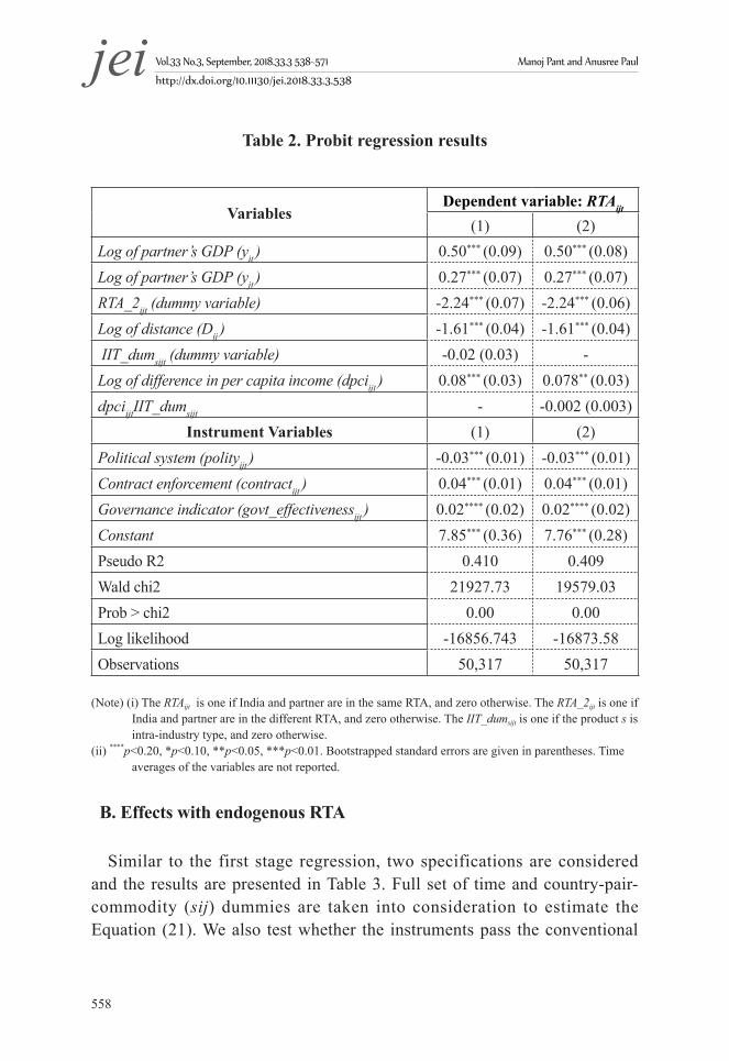
Vol.33 No.3, September, 2018.33.3 538~571� Manoj Pant and Anusree Paul
http://dx.doi.org/10.11130/jei.2018.33.3.538jei
558
Table 2. Probit regression results
VariablesDependent variable: RTAijt
(1) (2)Log of partner’s GDP (yit ) 0.50*** (0.09) 0.50*** (0.08)Log of partner’s GDP (yjt ) 0.27*** (0.07) 0.27*** (0.07)RTA_2ijt (dummy variable) -2.24*** (0.07) -2.24*** (0.06)Log of distance (Dij ) -1.61*** (0.04) -1.61*** (0.04) IIT_dumsijt (dummy variable) -0.02 (0.03) -Log of difference in per capita income (dpciijt ) 0.08*** (0.03) 0.078** (0.03)dpciijtIIT_dumsijt - -0.002 (0.003)
Instrument Variables (1) (2)Political system (polityijt ) -0.03*** (0.01) -0.03*** (0.01)Contract enforcement (contractijt ) 0.04*** (0.01) 0.04*** (0.01)Governance indicator (govt_effectivenessijt ) 0.02**** (0.02) 0.02**** (0.02)Constant 7.85*** (0.36) 7.76*** (0.28)Pseudo R2 0.410 0.409Wald chi2 21927.73 19579.03Prob > chi2 0.00 0.00Log likelihood -16856.743 -16873.58Observations 50,317 50,317
(Note) (i) The RTAijt is one if India and partner are in the same RTA, and zero otherwise. The RTA_2ijt is one if India and partner are in the different RTA, and zero otherwise. The IIT_dumsijt is one if the product s is intra-industry type, and zero otherwise.
(ii) ****p<0.20, *p<0.10, **p<0.05, ***p<0.01. Bootstrapped standard errors are given in parentheses. Time averages of the variables are not reported.
B. Effects with endogenous RTA
Similar to the first stage regression, two specifications are considered and the results are presented in Table 3. Full set of time and country-pair-commodity (sij) dummies are taken into consideration to estimate the Equation (21). We also test whether the instruments pass the conventional
The Role of Regional Trade Agreements: in the Case of India jei
559
overidentifying restrictions (Sargan-Hansen or OIR test). The high p-value of OIR test for each specification indicates that all instruments are significant determinants of RTA.12
To test the endogeneity of RTA for India, the joint significance between the coefficients of ĝ(.) and RTAijtĝ(.) is identified since they address the measure of potential endogeneity. The null hypothesis is H0:μ0 = μ1 = 0. Results show that corresponding Wald statistics are statistically significant at 5 percent level for both specifications (1) and (2), which ensures the endogeneity of RTA variable. The test statistics are reported in the Table 3. After accounting for selection bias, we find that the impact of RTA becomes insignificant, which indicates no impact of RTAs on India’s bilateral trade. In the context of other developing countries, studies of Sharma and Chua (2000), Lee and Park (2005), Pusterla (2007) have shown that RTAs have not created significant economic gains to the developing economies. Our results are not different.
Next, we concentrate on the regression results under the endogeneity of RTA. The directions of the controls are same as in the case of estimation results of model (11). But after accounting for the endogeneity or selection bias issue, the magnitudes are changed for the most of covariates. Market size effects on bilateral trade of India are more or less same as before. The trade diversion effect, coefficients of RTA_2ijt in both specifications (1) and (2), become stronger and significant at 1 percent level. Intra-industry trade increases by 45 percent which is much larger compared to estimation with exogeneous RTAs. Impact of factor endowment difference on trade is also higher but it is weakly significant. The marginal differential effect of factor endowment difference with respect to intra-industry trade type is further lowered by 0.995 on bilateral trade of India, but it increases by 1.3 for the RTA partner of India.
12 Further, the Cragg-Donald F-stat for FEIV is found sufficiently large which rejects the hypothesis of weak instruments at 5 percent level.

Vol.33 No.3, September, 2018.33.3 538~571� Manoj Pant and Anusree Paul
http://dx.doi.org/10.11130/jei.2018.33.3.538jei
560
Table 3. Two stage least square regression results
(Fixed effect)
VariablesLog of nominal bilateral trade
flow: ln(Xsijt+1)
(1) (2)RTAijt (dummy variable) -4.81 (14.89) -4.52 (15.49)Generalised residuals (ĝ(.)) 1.21*** (0.26) 1.21*** (0.31)RTAijtĝ(.) 0.53 (0.46) 0.51 (0.58)Log of partner’s GDP (yit ) 0.61*** (0.17) 0.60*** (0.16)Log of India’s GDP (y
jt ) 0.54*** (0.16) 0.530** (0.14)RTA_2ijt (dummy variable) -0.40*** (0.08) -0.40*** (0.09)IIT_dumsijt (dummy variable) 0.37*** (0.04)Log of difference in per capita income (dpciijt ) 1.04**** (0.67) 1.03* (0.59)dpciijtIIT_dumsijt 0.04*** (0.00)RTAijtdpciijtIIT_dumsijt -0.03*** (0.01)RTAijtyit 0.03 (0.21) 0.03 (0.19)RTAijtyjt 0.17 (0.18) 0.17 (0.22)RTAijtRTA_2ijt -0.23 (0.23) -0.22 (0.25)RTAijtIIT_dumsijt -0.31*** (0.08)RTAijtdpciijt -0.26**(0.12) -0.26***(0.09)RTAijtDij -0.10(0.08) -0.09(0.07)Constant -19.36**(7.70) -18.77***(7.16)Country-pair-Commodity FE Yes YesYear FE Yes YesSargan-Hansen OIR Test 0.627 0.606p-value of OIR Test 0.731 0.739Wald Chi2 (H0:μ0 = μ1 = 0) 24.55 23.53Prob > chi2 0.00 0.00Observations 50,317 50,317
(Note) (i) The RTAijt is one if India and partner are in the same RTA, and zero otherwise. The RTA_2ijt is one if India and partner are in the different RTA, and zero otherwise. The IIT_dumsijt is one if the product s is intra-industry type, and zero otherwise. The Dij is log of distance between countries. (ii) ****p<0.20, *p<0.10, **p<0.05, ***p<0.01. Bootstrapped standard errors are given in
parentheses. Time averages of the variables are not reported. Time invariant variable distance is omitted in fixed effect estimation results.

The Role of Regional Trade Agreements: in the Case of India jei
561
V. Concluding Remarks
The past literatures regarding the impact of RTAs on trade have simply assumed that the formation of RTAs is an exogenous variable. Furthermore, most gravity models are not derived from an underlying theoretical model and the coexistence of inter- and intra- industry trade is not considered. In this paper we try to eliminate this lacunae by developing the model which can reflect the coexistence of both trades and by estimating the model for India which has been fairly active in negotiating RTAs with developing countries in Asia since the year 2000.
The results indicate that when formation of RTAs is taken into account as endogeneous variable, the impact of India’s RTAs on its trade is statistically insignificant. The spurious significance that arises from a standard gravity model is due to a specification error so that the impact of the other factors on trade are incorrectly attributed to the RTA.
This provides interesting policy implications. India’s RTAs have not had any significant impact on promoting trade mainly because its trade with the RTA partners is very limited. In other words, what ensures the success of RTAs is the substantial trade volume prior to RTA. This leads to a rather surprising result that India would be better off when it negotiates RTAs with its major trading partners such as the USA, EU, China, the UAE etc. The intuition behind this is clear. Since India’s tariff level is higher than the most of RTA partners, tariff cuts after the RTA can bring greater benefits to the partner countries, probably leaving political resistance.
RTA by itself is not a trade promoting device.
Received 13 April 2018, Revised 30 July 2018, Accepted 27 August 2018
References
Adams, R., Dee, P., Gali, J. and McGuire, G. “The trade and investment effects of preferential trading arrangements—Old and new evidence.” Productivity

Vol.33 No.3, September, 2018.33.3 538~571� Manoj Pant and Anusree Paul
http://dx.doi.org/10.11130/jei.2018.33.3.538jei
562
Commission Staff Working Paper, Australian Government, Productivity Commission, Canberra, Australia (2003).
Akhter, N. and Ghani, E. “Regional Integration in South Asia: An Analysis of Trade Flows Using the Gravity Model.” The Pakistan Development Review 49(2) (2010): 105-118.
Anderson, James E. “A Theoretical Foundation for the Gravity Equation.” American Economic Review 69 (1) (1979): 106–116.
Anderson, J.E. and Marcouiller D. “Insecurity and The Pattern of Trade: An Empirical Investigation.” Review of Economics and Statistics 84 (2002):342-352.
Anderson, James E., vanWincoop, E. “Gravity with Gravitas: A Solution to The Border Puzzle.” American Economic Review 93 (1) (2003): 170–192.
Baccini, L. and Dür, A. “The new regionalism and policy interdependence.” British Journal of Political Science 42 (1) (2012):57-79.
Bagwell, K. and Staiger, Robert W. “Reciprocal Trade Liberalization.” NBER Working Paper No. 5488 (1996).
Bagwell, K. and Staiger, Robert W. “Multilateral Trade Negotiations, Bilateral Opportunism and the Rules of GATT.” NBER Working Paper No. 7071(1999).
Bagwell, K. and Staiger, R.“The World Trade Organization: Theory and Practice.” Annual Review of Economics 2(1) (2010): 223-256.
Baier, S. L., Bergstrand, J. H. “On the Endogeneity of International Trade Flows and Free Trade Agreements.” American Economic Association Annual Meeting (2002).
Baier, S. L., Bergstrand, J. H. “Economic Determinants of Free Trade
The Role of Regional Trade Agreements: in the Case of India jei
563
Agreements.” Journal of International Economics 64(1) (2004): 29–63.
Baier, S. L., Bergstrand, J. H. and Vidal, E. “Free Trade Agreements in the Americas: are the Trade Effects Larger than Anticipated?” World Economy 30(9) (2007):1347-77.
Baldwin, R.E. and Venables, A. J. (1995). “Regional Economic Integration” in Handbook of International Economics Vol. 3, Ed. Gene M. Grossman and Kenneth Rogoff (Elsevier, 1995, Amsterdam), 1597-1644.
Baldwin, R. “Managing the Noodle Bowl: The Fragility of East Asian Regionalism.” The Singapore Economic Review 53(3) (2008):449-478.
Bergstrand, J. “The Gravity Equation in International Trade: Some Macroeconomic Foundations and Empirical Evidence.” The Review of Economics and Statistics 6 (1985): 474-481.
Bergstrand, J. H. “The Generalized Gravity Equation, Monopolistic Competition, and the Factor-Proportions Theory in International Trade.” Review of Economics and Statistics 71(1) (1989): 143-153.
Bergstrand, J. H. “The Heckscher-Ohlin-Samuelson Model, the Linder Hypothesis and the Determinants of Bilateral Intra-industry Trade.” Economic Journal 100 (403) (1990):1216-29.
Beugelsdijk, S. and van Schaik, A.B.T.M. “Social Capital and Regional Economic Growth.” CentER Discussion Paper 2001-102. (2001). Available at: http://greywww.kub.nl:2080/greyfiles/center/2001/doc/102.pdf.
Bhagwati, J. Termites in the Trading System: How Preferential Agreements Undermine Free Trades, OUP, New Delhi (2008).
Burfisher, M. E., Robinson, S. and Thierfelder, K. “Developing Countries and The Gain from Regionalism.” American Journal of Agricultural Economics
Vol.33 No.3, September, 2018.33.3 538~571� Manoj Pant and Anusree Paul
http://dx.doi.org/10.11130/jei.2018.33.3.538jei
564
84(3) (2002):736-48.
Cabral, M., Falvey, R. and Milner, C. “Endowment Differences and the Composition of Intra-Industry Trade.” Research Paper 2008/36 Leverhulme Centre for GEP, University of Nottingham (2008).
Cernat, L. Assessing Regional Trade Arrangements: Are South-South RTAs More Trade Diverting. Policy Issues in International Trade and Commodities Study Series, No. 16 (2001).
Chang, W. and Winters, A. “How Regional Blocs Affect Excluded Countries: The Price Effects of MERCOSUR.” The American Economic Review 92(4) (2002): 889-904.
Clark D.P. and Stanley, D. L. “Determinants of Intra-Industry Trade Between Developing Countries and the United States.” Journal of Economic Development Volume 24 (2) (1999):79-95.
Coulibali, S. On the Complementarity of Regional and Global Trade. Washington, DC: World Bank. (2009). Available at: https://openknowledge.worldbank.org/handle/10986/9181 License: CC BY 3.0 IGO.
Davis, D.R. “Intra-industry trade: A Heckscher-Ohlin-Ricardo approach.” Journal of International Economics 39 (1995):201-226.
Deardorff, A. “Determinants of Bilateral Trade: Does Gravity Work in a Neoclassical World?” A chapter in The Regionalization of the World Economy, 7-32 from National Bureau of Economic Research, Inc. (1998).
Eaton, J. and Kortum, S. “Technology and Bilateral Trade.” NBER Working Paper No. 6253, National Bureau of Economic Research, (1997).
Egger, H., Egger, P. and Greenaway, D. “The Trade Structure Effects of Endogenous Regional Trade Agreements.” Journal of International Economics
The Role of Regional Trade Agreements: in the Case of India jei
565
74(2) (2008): 278–98.
Egger, P., Larch, M., Staub, K. E. and Winkelmann, R. “The Trade Effects of Endogenous Preferential Trade Agreements.” American Economic Journal: Economic Policy 3(2011): 113–143.
Estevadeordal, A. and Suominen, K. Bridging Regional Trade Agreements in the Americas, Inter-American Development Bank, (2009).
Falvey R. “Commercial Policy and Intra-Industry Trade.” Journal of International Economics 11(1981): 495-511.
Falvey, R.E., and Kierzkowski, H. “Product Quality, Intra-Industry Trade, and (Im)perfect Competition,” in Protection and Competition in International Trade: Essays in Honor of W.M. Corden, ed. by H. Kierzkowski, Oxford, Basil Blackwell (1987).
Fontagné L. and M. Freudenberg “Intra-Industry Trade: Methodological Issues Reconsidered.” CEPII Working Papers, #97-01, (1997).
Francois, J.F. and Shiells, C.R. “AGE Models of North American Free Trade”, in Modeling Trade Policy, Applied General Equilibrium Assessments of North American Free Trade, ed. Francois, J.F., Shiells, C.R., Cambridge University Press, Cambridge, (1994).
Frye, T. and Mansfield, E.D. “Timing is Everything: Elections and Trade Liberalization in the Postcommunist World.” Comparative Political Studies, 37 (4) (2004):371-398.
Grubel, H. and Peter Lloyd. Intra-industry trade, MacMillan, London, (1975).
Grossman G.M. and Helpman, E. “Protection for Sale.” American Economic Review 84(4) (1994):833-50.

Vol.33 No.3, September, 2018.33.3 538~571� Manoj Pant and Anusree Paul
http://dx.doi.org/10.11130/jei.2018.33.3.538jei
566
Grossman G.M., Helpman, E. “The Politics of Free-Trade Agreements.” American Economic Review 85(4) (1995):667-690.
Gullstrand, J. “Country-Specific Determinants of Vertical Intra-Industry Trade with Application to Trade Between Poland and EU”, in B. Wawrzynjak (ed.), Globalisation and Change – Ways to Future, Leon Kozminski Academy of Enterpreneurship and Management, Warsaw, (2000).
Helpman, E. “International Trade in the Presence of Product Differentiation, Economies of Scale, and Monopolistic Competition: A Chamberlin-HeckscherOhlin Approach.” Journal of International Economics 11(1981): 305-340.
Helpman, E. “Imperfect Competition and International Trade: Evidence from Fourteen Industrial Countries.” Journal of the Japanese and International Economies 6(1987):62-81.
Helpman, E., Krugman, P. “The Politics of Free Trade Agreements.” American Economic Review 85(1995): 667-690.
Henisz, W.J. and Mansfield, E.D. “Votes and Vetoes: The Political Determinants of Commercial Openness.” International Studies Quarterly 50 (1) (2006):189-212.
Joshi, V. “Econometric Analysis of India-Sri Lanka Free Trade Agreement.” Asian Economic Journal 26(2) (2012): 159–180.
Kandogan, Y. “Consistent estimates of regional blocs trade effects.” Review of International Economics 16(2) (2008): 301–314.
Krishna, P. “Regionalism and Multilateralism: A Political Economy Approach.” Quarterly Journal of Economics113 (1998):227-51.
Krugman, P.R. “Increasing returns, monopolistic competition, and international
The Role of Regional Trade Agreements: in the Case of India jei
567
trade.” Journal of international Economics 9(4) (1979): 469-479.
Lee, Jong-Wha. and Park, I. “Free Trade Areas in East Asia: Discriminatory or Non-discriminatory.” The World Economy 28(1) (2005):21-48.
Lewis-Beck, M.S. Economics and Elections: The Major Western Democracies. Ann Arbor, MI: University of Michigan Press, (1988).
Liu, X. “The Political Economy of Free Trade Agreements: An Empirical Investigation.” Journal of Economic Integration 23(2) (2008): 237-271.
Liu, X. “Testing Conflicting Political Economy Theories: Full-fledged vs. Partial-scope Regional.” Southern Economic Journal 77(1) (2010): 78-103.
Mansfield, E. D., Helen V. M. and Rosendorff, B. P. “Why Democracies Cooperate More: Electoral Control and International Trade Agreements.” International Organization 56 (2002): 477-514.
MacPhee, C.R. and Sattayanuwat, W. “Consequence of Regional Trade Agreements to Developing Countries.” Journal of Economic Integration 29(1) (2014): 64-94.
Magee, C. S. P. “Endogenous Preferential Trade Agreements: An Empirical Analysis.” Contributions to Economic Analysis and Policy 2(1) (2003).
Magee, C. S. P. “Trade Creation, Trade Diversion, and Endogenous Regionalism.” Econometric Society, North American Summer Meetings, Series number 289 (2004).
Maggi, G. and Rodríguez-Clare, A. “The Value of Trade Agreements in the Presence of Political Pressures.” Journal of Political Economy 106(3) (1998): 574-601.
Maggi, G. and Rodríguez-Clare, A. “A Political-Economy Theory of Trade

Vol.33 No.3, September, 2018.33.3 538~571� Manoj Pant and Anusree Paul
http://dx.doi.org/10.11130/jei.2018.33.3.538jei
568
Agreements.” American Economic Review 97(4) (2007):1374-1406.
Mansfield, E. (1998). “The Proliferation of Preferential Trading Agreements.” Journal of Conflict Resolution 42(5):523-43.
Mansfield, E. D., Milner, H.V. and Rosendorff, B. P. “Why Democracies Cooperate More: Electoral Control and International Trade Agreements.” International Organization 56 (3) (2002):477-513.
Markusen, J. R. “Explaining the Volume of Trade: An Eclectic Approach.” The American Economic Review 76(5) (1986):1002-1011.
Milner, H. V. and Kubota, K. “Why the Move to Free Trade? Democracy and Trade Policy in the Developing Countries.” International Organization 59(1) (2005):107-143.
Mitra, D., Thomakos, D.D. and Ulubaşoglu, M. A. “‘Protection for Sale’ in a Developing Country: Democracy vs. Dictatorship.” The Review of Economics and Statistics 84 (3) (2002): 497-508.
Mundlak, Y. “On the pooling of time series and cross section data.” Econometrica 46 (1978):69-85.
Murtazashvili, I. and Wooldridge, J. M. “A control function approach to estimating switching regression models with endogenous explanatory variables and endogenous switching.” Journal of Econometrics 190(2) (2016): 252-266.
Pant, M., Sadhukhan, A. “Does Regionalism Hinder Multilateralism: A Case study of India.” Journal of Economic Integration 24(2) (2009): 222-247.
Pant, M. “Regional Trading Arrangements and Developing Countries: Understanding the Phenomena.” International Studies 47(2–4) (2010): 187–203.
The Role of Regional Trade Agreements: in the Case of India jei
569
Pusterla, F. “Regional Integration Agreements: Impact, Geography and Efficiency.” IDB-SOE Working Paper No. 1, (2007).
Robinson, S. and Thierfelder, K. “Trade Liberalisation and Regional Integration: The Search for Large Numbers.” The Australian Journal of Agricultural and Resource Economics 46(4) (2002):585–604.
Schiff, M. and Winters, L. Alan. Regional Integration and Development, A co-publication of the World Bank and Oxford University Press (2003).
Semykina, A. and Wooldridge, J.M. “Estimating panel data models in the presence of endogeneity and selection.” Journal of Econometrics 157(2) (2010): 375-380.
Sen, R., Srivastava, S. and Webber, D. “Preferential trading agreements and the gravity model in presence of zero and missing trade flows: Early results for China and India.” Working Papers 2015-02, Auckland University of Technology, Department of Economics, (2015).
Shahid, A. “India-Korea CEPA: An Assessment.” Korea and the World Economy 12(1) (2011):45–98.
Sharma, S. C. and Chua, S. Y. “ASEAN: Economic Integration and Intra-Regional Trade.” Applied Economics Letters 7(3) (2000):165-69.
Srinivasan, T.N. and Archana, Vani. “India in the Global and Regional Trade: Determinants of Aggregate and Bilateral Trade Flows and Firms- Decision to Export”. Working Paper No. 232, Indian Council for Research on International Economic Relations, (2009).
Taneja, N., Ray, S. and Pande, D. “India – Pakistan Trade: Textiles and Clothing.” Working Paper 326, Indian Council for Research on International Economic Relations, (2016).
Vol.33 No.3, September, 2018.33.3 538~571� Manoj Pant and Anusree Paul
http://dx.doi.org/10.11130/jei.2018.33.3.538jei
570
Veeramani, C. “India’s Intra-Industry Trade under Economic Liberalisation: Trends and Country Specific Factors.” CDS Working Paper No. 313, Trivandrum: Centre for Development Studies (2001).
Verdier, D. “Democratic Convergence and Free Trade.” International Studies Quarterly 42 (1) (1998): 1-24.
Viner, J. The Customs Union Issue. New York: Carnegie Endowment for International Peace, (1950).
Wignaraja, G. “PRC and India: Pursuing the Same Approach to Free Trade Agreements?”, Asia Pathways, ADBI (2012). accessed online at http://www.asiapathways-adbi.org/2012/10/prc-and-india-pursuing-the-same-approach-to-free-trade-agreements/
Winters, L. “Regionalism versus Multilateralism.” Policy Research Working Paper Series No 1687, World Bank (1996).
Winters, L. A. “What can European Experience Teach Developing Countries about Integration?” World Economy 20(7) (1997): 889–912.
Winters, L. A. and Chang, W. “Regional Integration and Import Prices: An Empirical Investigation.” Journal of International Economics 51(2010):363-377.
Wooldridge, J. M. “Selection corrections for panel data models under conditional mean independence assumptions.” Journal of Econometrics 68 (1) (1995): 115-132.
Wooldridge, J. M. Econometric Analysis of Cross Section and Panel Data. 2nd edition, The MIT Press. Cambridge, Massachusetts. London, England (2002).
World Bank. Trade Blocs. Policy Research Report. New York: Oxford University Press (2000).
The Role of Regional Trade Agreements: in the Case of India jei
571
Yeats, A. “Does Mercosur’s Trade Performance Raise Concerns about the effects of Regional Trade Arrangements?” World Bank Economic Review 12(1) (1998): 1 – 28.