8 February 2012

The Role of Profits and Income in the Statistical Discrepancy By Dylan G. Rassier

THE NATIONAL income and product accounts (NIPAs) of the Bureau of Economic Analysis

(BEA) include two alternative measures of economic output: gross domestic product (GDP) and gross do­mestic income (GDI). GDP is an expenditure-based measure and is estimated based on spending on final goods and services. GDI is an income-based measure and is estimated based on income generated in the production of goods and services. Before the recession that began in the fourth quarter of 2007 and ended in the second quarter of 2009, GDI growth was generally lower than GDP growth, which has generated discus­sion about whether the source data and adjustments that underlie GDP reflect enough economic cyclicality. This article explores an alternative: whether the source data and adjustments that underlie GDI reflect too much economic cyclicality and whether this effect may explain a significant share of the difference between GDP and GDI during the downturn. In particular, this article identifies and explains the following four factors that require adjustments to convert financial- or tax-based source data into economic accounting measures of corporate profits and proprietors’ and partnership income (hereafter, profits and income):

● Misreporting on tax returns comprises a significant portion of profits and income, and while there may be reasons to think that misreporting would be cyclical in nature, long-term enforcement efforts may well offset any cyclicality in reporting, and the overall cyclical effect of adjustments for misreport­ing is ambiguous.

● Capital gains and losses may be leaking into mea­sures of profits and income, which could yield overly cyclical measures of profits and income.

● Inconsistent measurement of stock options in source data may generate an overly cyclical measure of GDI relative to GDP.

● Assumptions regarding the capitalization rate of purchased software may overstate profits and income during cyclical upturns. For each of these factors, additional research is war­

ranted and ongoing to understand the potential con­

tribution of each factor to differences between GDP and GDI.

BEA prepares current quarterly estimates and an­nual estimates of GDP and GDI, each of which is sub­ject to several revisions.1 Each revision yields a new vintage of estimates. Each successive current quarterly vintage incorporates newly available source data. Each annual vintage incorporates newly available source data as well as improved estimating methodologies. In addition to revising annual estimates, an annual revi­sion includes revisions to the quarterly estimates. Ap­proximately every 5 years, BEA prepares a benchmark revision, which incorporates newly available, compre­hensive source data, improved estimating methodolo­gies, and definition changes.

In concept, GDP and GDI are equal because expen­ditures by one party in the economy become income to another party. In practice, all vintages of GDP and GDI are estimated from largely independent and incom­plete source data, so the errors in each measure are not the same. Vintages face tradeoffs between timeliness and accuracy. While current quarterly vintages offer the timeliest look at economic output, the accuracy of current quarterly vintages is affected more than the ac­curacy of later vintages by the completeness and reli­ability of the underlying source data. Annual and benchmark revisions improve accuracy, but the result­ing vintages are less timely than the current quarterly vintages.2 Regardless of the vintage, discrepancies between GDP and GDI are introduced through

1. There are three current quarterly vintages for each quarter: advance, second, and third. Advance, second, and third quarterly vintages are released approximately 1, 2, and 3 months, respectively, after the end of the reference quarter. Likewise, there are three annual vintages for each year: first, second, and third. Annual vintages are released at the end of July for the previous 3 years. The most recent vintage of annual estimates comes from the 2011 annual revision, which was released on July 29, 2011. The 2011 annual revision includes the first annual revision for 2010, the second for 2009, and the third for 2008. In addition, the 2011 annual revision was the first “flexible” annual revision, which includes revisions to current-dol­lar GDP and some components back to the first quarter of 2003.

2. However, revision studies generally conclude that annual and bench­mark revisions do not substantively change BEA’s measures of long-term growth, pictures of business cycles, and trends in major components of GDP (Fixler, Greenaway-McGrevy, and Grimm 2011).

9 February 2012 SURVEY OF CURRENT BUSINESS

differences in source data, adjustments of source data to economic concepts and definitions, differences in interpolation and extrapolation techniques, and differences in the timing of quarterly seasonal adjustments. Thus, even after annual and benchmark revisions are incorporated, differences between GDP and GDI persist in annual and quarterly estimates. However, recent work shows that GDP and GDI levels follow the same trend and rarely drift far from each other (Greenaway-McGrevy 2011).

The difference between GDP and GDI is known as the statistical discrepancy. Both GDP and GDI provide a complete picture of economic output, so the statisti­cal discrepancy provides an indication of net measure­ment error. In addition, changes in the degree and direction of the statistical discrepancy from one period to another reflect differences in the rates of growth be­tween GDP and GDI. Internationally, statistical agen­cies generally choose one of two alternatives to handle the statistical discrepancy. One alternative is to publish a statistical discrepancy as a separate line item in the national accounts based on the relative reliability of the underlying source data. A second alternative is to allo­cate the discrepancy to the components of output where measurement errors are most likely to exist.3

BEA follows the first alternative and publishes a statis­tical discrepancy as a line item with aggregate GDI. The resulting double-entry accounts yield a break­down by component of GDP and GDI in addition to an indication of the consistency between the two sides of the accounts.

BEA recognizes strengths and weaknesses of both GDP and GDI as measures used to analyze economic activity and business cyclicality. However, a decision ultimately has to be made regarding which side of the national accounts to record the statistical discrepancy. Given the important role that corporate profits and proprietors’ and partnership income play as compo­nents of GDI and given the challenges of adjusting source data to accord with economic accounting mea­sures of profits and income, BEA records the statistical discrepancy with GDI in order to reflect the relative re­liability of the source data and required adjustments underlying GDI relative to GDP. Thus, this article fo­cuses on income-side factors and adjustments that have led to concern at BEA about possible measure­

3. For the first alternative, the System of National Accounts 2008 (SNA) suggests “. . . it is usual to attach [the discrepancy] to the variant of [national output] the office feels is least accurate. The aim is to show users something about the degree of reliability of the published data” (SNA paragraph 18.16). For the second alternative, the SNA suggests “The alternative is for the office to remove the discrepancy by examining the data in the light of the many accounting constraints in the SNA, making the best judgment possible about where the errors are likely to have arisen and modifying the data accordingly” (SNA paragraph 18.17).

ment error. In particular, this article focuses on the re­cent behavior of the statistical discrepancy and potential cyclicality of the measurement error in prof­its and income.

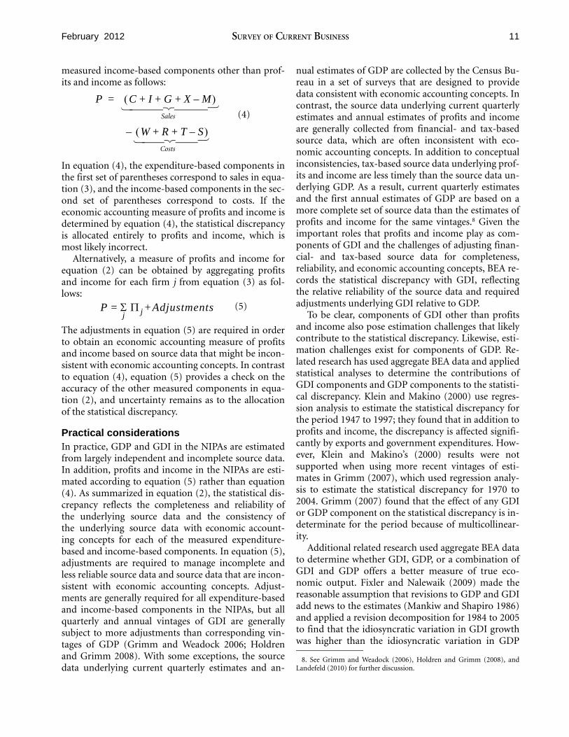
Table 1 shows the component shares of GDI for the 5-year period from 2006 to 2010 using quarterly BEA data from the 2011 annual revision of the NIPAs, which provides the most recent vintage of estimates. This period includes the most recent recession (from the fourth quarter of 2007 to the second quarter of 2009) as determined by the Business Cycle Dating Committee of the National Bureau of Economic Re­search (NBER). Profits and income generally account for 15 to 20 percent of GDI. Table 1 shows that profits declined sharply through the fourth quarter of 2008, and income declined slightly through the second quar­ter of 2009. The declines in profits and income were offset in part by increases in the shares of compensa­tion, other net operating surplus, and consumption of fixed capital. Table 1 does not provide insight regard­ing measurement error but does indicate profits and income account for a larger-than-proportionate share of any declines in GDI during the recession.4

In addition to profits and income, other compo­nents of GDI are subject to measurement error. Like­wise, measurement error affects all components of GDP. As a result, some recent studies have questioned BEA’s decision to record the statistical discrepancy with GDI and the resulting emphasis on GDP in news

4. A similar perspective of GDP for the same period indicates a sharp decrease in private investment, which is offset in part by increases in net exports and government expenditures and gross investment.

Table 1. Component Shares of Gross Domestic Income, 2006–2010 [Percent]

Compen­sation

Taxes less subsidies

Proprietors’ income

Corporate profits

Other net operating surplus

Consump­tion of fixed

capital

2006: I ........... 55.0 6.9 8.4 10.0 7.5 12.1 II .......... 54.9 6.9 8.4 9.9 7.8 12.2 III ......... 54.7 6.8 8.3 10.2 7.8 12.2 IV......... 55.3 6.8 8.2 9.5 7.8 12.3

2007: I ........... 55.7 6.9 7.9 8.8 8.2 12.5 II .......... 55.7 6.9 7.8 8.9 8.2 12.5 III ......... 56.1 6.9 7.7 8.0 8.5 12.7 IV......... 56.4 6.9 7.7 7.3 8.9 12.7

2008: I ........... 56.6 6.8 7.8 6.6 9.5 12.7 II .......... 56.2 6.9 7.8 6.4 9.9 12.8 III ......... 56.2 6.9 7.7 6.2 10.1 13.0 IV......... 57.1 6.9 7.4 4.4 10.8 13.4

2009: I ........... 56.6 6.9 6.9 5.9 10.1 13.6 II .......... 56.8 7.0 6.7 6.7 9.3 13.6 III ......... 56.4 6.9 6.7 7.8 8.8 13.4 IV......... 55.8 7.0 6.8 8.5 8.7 13.3

2010: I ........... 55.0 6.9 6.9 9.5 8.7 13.0 II .......... 55.1 6.9 7.1 9.6 8.4 12.9 III ......... 55.0 6.8 7.2 9.8 8.3 12.9 IV......... 54.7 6.8 7.3 10.1 8.1 12.9

NOTES. The shaded area is the date of the recession determined by the Business Cycle Dating Committee of the National Bureau of Economic Research. GDI components are from NIPA table 1.10. The data are from the 2011 annual NIPA revision.

10 Statistical Discrepancy February 2012

releases (for example, see Klein and Makino 2000; Fix­ler and Nalewaik 2009; Nalewaik 2010). As a steward of the U.S. national accounts, BEA does not intend to promote one measure over another, and the recent work generally supports BEA’s conclusion that both GDP and GDI are valid measures of output. However, how much each measure might be weighted in a com­bined measure and whether temporal variation should be assumed to indicate less reliability or more reliabil­ity remains unresolved and, in some cases, may run contrary to other studies (for example, see Weale 1992; Smith, Weale, and Satchell 1998; Grimm and Parker 1998; Fixler and Grimm 2002 2005; and Greenaway-McGrevy 2011). In addition, most of the work to date on combining GDP and GDI focuses on weighting ag­gregate measures rather than on weighting the under­lying source data. As an alternative, BEA is currently conducting research on weighting the underlying source data based on reliability in a model to distribute the statistical discrepancy before aggregating the com­ponent estimates (for example, see Chen 2006, 2010). While weighting the underlying source data receives strong support from a theoretical perspective (for ex­ample, see Stone, Meade, and Champernowne 1942; Byron 1978), the practicality and feasibility of weight­ing the underlying source data have yet to be deter­mined.5

The first section presents an accounting framework to describe the role of profits and income in the statis­tical discrepancy. The section also discusses empirical evidence to explain the focus on profits and income rather than on other components of GDI and GDP. The next section identifies and explains the factors of profits and income that are most likely to contribute to the statistical discrepancy. The final section offers some concluding observations.

Profits and Income and the Statistical Discrepancy

Accounting framework To provide some conceptual context, we follow Klein and Makino’s (2000) construction of the national ac­counting identity.6 The expenditure-based measure of

5. Weighting underlying source data in a statistical framework has been successfully implemented at BEA to reconcile and balance the gross operat­ing surplus component of the 2002 input-output accounts and GDP by industry accounts (Rassier et al. 2007).

6. Klein and Makino (2000) argue that BEA’s decision to record the statis­tical discrepancy with GDI is tenable but may result in nonrandom error in the NIPAs. As a result, the authors argue that the statistical discrepancy should be distributed among the components of GDP and GDI. While their conclusions are subject to question (see Grimm 2007), their analytic frame­work is uncontroversial and useful to explain BEA’s decision to record the statistical discrepancy with GDI.

output can be written as the sum of consumer expen­ditures (C), investment (I), government expenditures (G), and exports (X) less imports (M). Likewise, the income-based measure of output can be written as the sum of wages (W), profits and income (P), rents and interest (R), and taxes on production (T) less subsidies (S). Thus, if all these variables are measured in accor­dance with economic accounting principles, the ac­counting identity for output is as shown in the following equation:

C + I + G + X – M (1) = W + + + P R T – S

The left side of equation (1) captures all final expen­ditures on goods and services in the economy, and the right side captures all income accruing to the input factors used for the production of the goods and ser­vices. The asterisks in equation (1) indicate compo­nents measured without error. In practice, each of the components is usually estimated from independent and incomplete source data. In addition, at least some of the components in equation (1) are estimated from source data that are not consistent with economic ac­counting concepts and thus require adjustments. Thus, the identity is inevitably not satisfied, resulting in a sta­tistical discrepancy (SD) as follows:

SD = C I G X M + + + –(2)

– W P R T S + + + – In equation (2), asterisks are removed to reflect mea­surement error in each of the components.

Klein and Makino (2000) point out that firm-level profits and income are never directly estimable but are merely a residual between sales and costs as follows:7

= Sales – Costs (3)

From a financial accounting perspective, the results of equation (3) may vary across firms because of flexibil­ity in the application of financial accounting rules. Likewise, the results of equation (3) may vary between financial and tax accounting records within a firm be­cause of differences between financial and tax account­ing rules.

From an economic accounting perspective, a mea­sure of profits and income from equation (2) can be obtained by calculating the residual between the measured expenditure-based components and the

7. We use different notation for profits and income in equation (3) than in equation (1) because P in equation (1) denotes aggregate profits and income that are consistent with economic accounting concepts while in equation (3) denotes firm-level profits and income that are consis­

tent with financial or tax accounting concepts.

11 February 2012 SURVEY OF CURRENT BUSINESS

measured income-based components other than prof- nual estimates of GDP are collected by the Census Bu­its and income as follows: reau in a set of surveys that are designed to provide

data consistent with economic accounting concepts. In P = C + + + I G X – M

contrast, the source data underlying current quarterly Sales (4) estimates and annual estimates of profits and income

are generally collected from financial- and tax-based W R T S+ + – – source data, which are often inconsistent with eco­

Costs

In equation (4), the expenditure-based components in the first set of parentheses correspond to sales in equa­tion (3), and the income-based components in the sec­ond set of parentheses correspond to costs. If the economic accounting measure of profits and income is determined by equation (4), the statistical discrepancy is allocated entirely to profits and income, which is most likely incorrect.

Alternatively, a measure of profits and income for equation (2) can be obtained by aggregating profits and income for each firm j from equation (3) as fol­lows:

nomic accounting concepts. In addition to conceptual inconsistencies, tax-based source data underlying prof­its and income are less timely than the source data un­derlying GDP. As a result, current quarterly estimates and the first annual estimates of GDP are based on a more complete set of source data than the estimates of profits and income for the same vintages.8 Given the important roles that profits and income play as com­ponents of GDI and the challenges of adjusting finan­cial- and tax-based source data for completeness, reliability, and economic accounting concepts, BEA re­cords the statistical discrepancy with GDI, reflecting the relative reliability of the source data and required adjustments underlying GDI relative to GDP. P= j +Adjustments (5)

j To be clear, components of GDI other than profits and income also pose estimation challenges that likely contribute to the statistical discrepancy. Likewise, esti­mation challenges exist for components of GDP. Re­lated research has used aggregate BEA data and applied statistical analyses to determine the contributions of GDI components and GDP components to the statisti­cal discrepancy. Klein and Makino (2000) use regres-

The adjustments in equation (5) are required in order to obtain an economic accounting measure of profits and income based on source data that might be incon­sistent with economic accounting concepts. In contrast to equation (4), equation (5) provides a check on the accuracy of the other measured components in equa­tion (2), and uncertainty remains as to the allocation

sion analysis to estimate the statistical discrepancy for of the statistical discrepancy. the period 1947 to 1997; they found that in addition to

Practical considerations In practice, GDP and GDI in the NIPAs are estimated from largely independent and incomplete source data. In addition, profits and income in the NIPAs are esti­mated according to equation (5) rather than equation (4). As summarized in equation (2), the statistical dis­crepancy reflects the completeness and reliability of the underlying source data and the consistency of the underlying source data with economic account­ing concepts for each of the measured expenditure-based and income-based components. In equation (5), adjustments are required to manage incomplete and less reliable source data and source data that are incon­sistent with economic accounting concepts. Adjust­ments are generally required for all expenditure-based and income-based components in the NIPAs, but all quarterly and annual vintages of GDI are generally subject to more adjustments than corresponding vin­tages of GDP (Grimm and Weadock 2006; Holdren and Grimm 2008). With some exceptions, the source data underlying current quarterly estimates and an-

profits and income, the discrepancy is affected signifi­cantly by exports and government expenditures. How­ever, Klein and Makino’s (2000) results were not supported when using more recent vintages of esti­mates in Grimm (2007), which used regression analy­sis to estimate the statistical discrepancy for 1970 to 2004. Grimm (2007) found that the effect of any GDI or GDP component on the statistical discrepancy is in­determinate for the period because of multicollinear­ity.

Additional related research used aggregate BEA data to determine whether GDI, GDP, or a combination of GDI and GDP offers a better measure of true eco­nomic output. Fixler and Nalewaik (2009) made the reasonable assumption that revisions to GDP and GDI add news to the estimates (Mankiw and Shapiro 1986) and applied a revision decomposition for 1984 to 2005 to find that the idiosyncratic variation in GDI growth was higher than the idiosyncratic variation in GDP

8. See Grimm and Weadock (2006), Holdren and Grimm (2008), and Landefeld (2010) for further discussion.

12 Statistical Discrepancy February 2012

growth after revisions. Fixler and Nalewaik (2009) at­tributed the increased variation in GDI growth to news and concluded that GDI should be weighted more than GDP in a combined measure of output without suggesting a combination of appropriate weights. In addition, Nalewaik (2010) applied statistical tests to determine whether growth in GDP or GDI better re­flects business cyclicality in output growth for 1978 to 2009, and the study concluded that GDI growth is a better measure of cyclicality without providing a rigor­ous analysis for a weighted measure of output.

Greenaway-McGrevy (2011) applied a Kalman filter to determine true economic output for the period 1983–2009 and concludes that the measurement error of GDP is smaller than the measurement error of GDI. Greenaway-McGrevy (2011) suggested that GDP should be weighted approximately 60 percent and GDI should be weighted approximately 40 percent in a combined measure of output.

Other related research used disaggregated BEA data to determine the distribution of the statistical discrep­ancy to GDI and GDP components. Chen (2010) ap­plied a generalized least squares (GLS) model to distribute the statistical discrepancy in 2002 to the components of expenditure-based GDP in the NIPAs, the components of value added in the income-based GDP by industry accounts, and the gross output and intermediate inputs of the input-output accounts based on the relative reliabilities of underlying source data in all the accounts. She found that the optimal ad­justments to gross output, intermediate inputs, and GDP components are relatively small, while the opti­mal adjustments to value added are relatively large due to the relatively low reliability of tax-based source data and adjustments included in the gross operating sur­plus component of value added.9 In earlier work, Chen (2006) applied a GLS model to distribute the statistical discrepancy in 1997 to the components of value added in the income-based GDP by industry accounts and to gross output and intermediate inputs of the input-out­put accounts. In contrast to Chen (2010), the compo­nents of expenditure-based GDP were held fixed in Chen (2006). Similar to Chen (2010), Chen (2006) found relatively small adjustments to gross output and intermediate inputs and relatively large adjustments to value added given the relative reliabilities of the under­lying data.

9. Corporate profits, proprietors’ income, and partnership income consti­tute a large proportion of gross operating surplus.

In sum, the studies that used disaggregated data with statistical analyses have yielded a consistent set of results and conclusions, whereas studies that used ag­gregated data with statistical analyses have so far yielded a mixed set of results and conclusions. In other words, a bottom-up approach may be necessary to draw conclusions about the extent to which the statis­tical discrepancy is likely to be attributable to expendi­ture-based and income-based components. Thus, from a practical perspective, BEA must rely on its experience with underlying source data in its decision to record the statistical discrepancy with GDI.

Cyclicality The behavior of the statistical discrepancy may look different on a quarterly basis than on an annual basis because quarterly variation is netted out in annual esti­mates.10 The behavior of the statistical discrepancy during cyclical turning points is particularly important to policymakers and other decisionmakers because dif­ferences between GDP and GDI can complicate the de­cisionmaking process. Likewise, when it comes to making real-time decisions, current quarterly vintages of GDP and GDI are timelier than vintages based on annual and benchmark revisions. Regardless of the vintage, the cyclicality of underlying source data and required adjustments affecting GDP and GDI is im­portant to consider in the decision about where to re­cord the statistical discrepancy because source data and adjustments that are overly cyclical or not cyclical enough are likely to yield a less accurate measure of economic output.

Chart 1 presents the quarterly statistical discrepancy as a percent of GDP for the 5-year period 2006–2010. This period includes the recession that began in the fourth quarter of 2007 and ended in the second quar­ter of 2009, as determined by NBER’s Business Cycle Dating Committee. Before the recession that began in 2007, the quarterly statistical discrepancy changes from relatively large and negative in the first quarter to relatively large and positive by the last quarter. With the exception of the period from the first quarter of 2006 to the first quarter of 2007, the quarterly statisti­cal discrepancy as a percent of GDP is less than 1 per­cent.

10. While first annual estimates are generally based on the same source data used for quarterly interpolations and extrapolations, second and third annual estimates are based on tax-based source data. Thus, quarterly varia­tion related to the second and third annual estimates comes from the source data used for quarterly interpolations.

13 February 2012 SURVEY OF CURRENT BUSINESS

Chart 2 presents real GDP levels and real GDI lev- creases slightly in the first quarter of 2008 before de­els.11 The difference between the two series reflects the creasing significantly during the remaining quarters of variation in the statistical discrepancy as shown in the recession. At both the NBER peak and the NBER chart 1. As shown in chart 2, real GDI is generally trough, real GDI is lower than real GDP. Real GDP in-higher than real GDP before the third quarter of 2007 creases consistently in the quarters preceding the but relatively flat for the three quarters leading to the NBER peak in 2007 but decreases slightly for the first NBER peak in the fourth quarter of 2007. Real GDI in- quarter of 2008 before increasing slightly and then de­

creasing significantly during the remaining quarters of 11. Real GDP and real GDI are published in chained 2005 dollars. We

the recession.deflate current-dollar GDI using the implicit price deflator for GDP because there is no price deflator specifically for GDI.

Chart 1. Quarterly Statistical Discrepancy as a Percent of GDP, 2006–2010 Statistical discrepancy/GDP

NBER National Bureau of Economic Research NOTES. The statistical discrepancy and GDP are from NIPA tables 1.10 and 1.1.5, respectively. The data are from the 2011 annual NIPA revision.

U.S. Bureau of Economic Analysis

0.010

0.005

0.00

–0.005

–0.010

–0.015

–0.020

–0.025 2006 2007 2008 2009 2010

NBER peak NBER trough

CharChartt 2.2. QuarQuartterlerlyy Real GDP and Real GDI LeReal GDP and Real GDI Levels,vels, 2006–20102006–2010

NBER National Bureau of Economic Research NOTES. Real GDP levels are from NIPA table 1.1.6. Real GDI levels are derived by deflating current-dollar GDI from NIPA table 1.10 by the implicit price deflator for GDP from NIPA table 1.1.9. The data are from the 2011 annual revision.

U.S. Bureau of Economic Analysis

2006 2007 2008 2009 2010

NBER peak NBER trough

Billions of dollars 13,400

13,300

13,200

13,100

13,000

12,900

12,800

12,700

12,600

12,500

12,400

GDI

GDP

14 Statistical Discrepancy February 2012

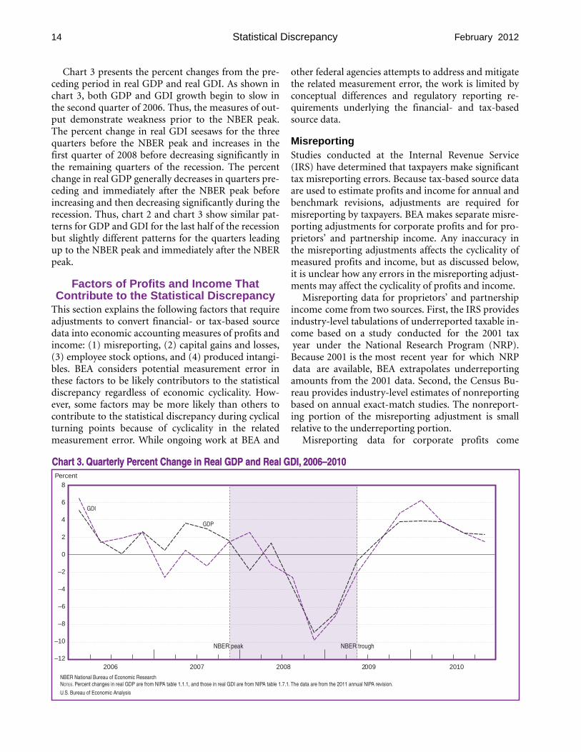
Chart 3 presents the percent changes from the pre­ceding period in real GDP and real GDI. As shown in chart 3, both GDP and GDI growth begin to slow in the second quarter of 2006. Thus, the measures of out­put demonstrate weakness prior to the NBER peak. The percent change in real GDI seesaws for the three quarters before the NBER peak and increases in the first quarter of 2008 before decreasing significantly in the remaining quarters of the recession. The percent change in real GDP generally decreases in quarters pre­ceding and immediately after the NBER peak before increasing and then decreasing significantly during the recession. Thus, chart 2 and chart 3 show similar pat­terns for GDP and GDI for the last half of the recession but slightly different patterns for the quarters leading up to the NBER peak and immediately after the NBER peak.

Factors of Profits and Income That Contribute to the Statistical Discrepancy

This section explains the following factors that require adjustments to convert financial- or tax-based source data into economic accounting measures of profits and income: (1) misreporting, (2) capital gains and losses, (3) employee stock options, and (4) produced intangi­bles. BEA considers potential measurement error in these factors to be likely contributors to the statistical discrepancy regardless of economic cyclicality. How­ever, some factors may be more likely than others to contribute to the statistical discrepancy during cyclical turning points because of cyclicality in the related measurement error. While ongoing work at BEA and

other federal agencies attempts to address and mitigate the related measurement error, the work is limited by conceptual differences and regulatory reporting re­quirements underlying the financial- and tax-based source data.

Misreporting Studies conducted at the Internal Revenue Service (IRS) have determined that taxpayers make significant tax misreporting errors. Because tax-based source data are used to estimate profits and income for annual and benchmark revisions, adjustments are required for misreporting by taxpayers. BEA makes separate misre­porting adjustments for corporate profits and for pro­prietors’ and partnership income. Any inaccuracy in the misreporting adjustments affects the cyclicality of measured profits and income, but as discussed below, it is unclear how any errors in the misreporting adjust­ments may affect the cyclicality of profits and income.

Misreporting data for proprietors’ and partnership income come from two sources. First, the IRS provides industry-level tabulations of underreported taxable in­come based on a study conducted for the 2001 tax year under the National Research Program (NRP). Because 2001 is the most recent year for which NRP data are available, BEA extrapolates underreporting amounts from the 2001 data. Second, the Census Bu­reau provides industry-level estimates of nonreporting based on annual exact-match studies. The nonreport­ing portion of the misreporting adjustment is small relative to the underreporting portion.

Misreporting data for corporate profits come

CharChartt 3.3. QuarQuartterlerlyy PPeerrcent Changcent Change in Real GDP and Real GDI,e in Real GDP and Real GDI, 2006–20102006–2010 Percent

NBER National Bureau of Economic Research NOTES. Percent changes in real GDP are from NIPA table 1.1.1, and those in real GDI are from NIPA table 1.7.1. The data are from the 2011 annual NIPA revision.

U.S. Bureau of Economic Analysis

8

6

4

2

0

–2

–4

–6

–8

–10

–12

NBER peak NBER trough

GDI

GDP

2006 2007 2008 2009 2010

15 February 2012 SURVEY OF CURRENT BUSINESS

primarily from annual IRS corporate audit reports, which provide estimates of additional tax amounts owed as determined through audits. BEA supplements the audit reports with IRS tabulations of the amounts actually collected versus the amounts recommended in the audit reports. To determine misreported profits, BEA makes judgments regarding marginal tax rates. In addition, given the nonrandom nature of the audit sample, BEA makes judgments regarding the applica­tion of the audit amounts to the universe of corpora­tions.

Given the patchwork of misreporting source data and the age of some misreporting source data, BEA considers the misreporting adjustments to be of rela­tively low reliability for assessing year-to-year changes. In addition, the misreporting adjustments comprise a significant amount of corporate profits and propri­etors’ and partnership income. As a percent of propri­etors’ and partnership income in the NIPAs, the misreporting adjustments for proprietors and partner­ships have been approximately 50 percent since 1970. As a percent of profits before taxes in the NIPAs, the misreporting adjustments for corporations have gener­ally fluctuated between 15 and 25 percent. Thus, the misreporting adjustments for proprietors and partner­ships are generally larger as a percent than the misre­porting adjustments for corporations.

BEA does not make any explicit cyclical adjustments to its overall misreporting adjustments. This is in part due to uncertainty about the potential effect of cycli­cality on misreporting. For example, if misreporting increases during a downturn as businesses attempt to retain a larger after-tax share of their business income, the decline in profits and income could be overstated during the downturn. However, long-term efforts by the IRS to increase the number of examinations and audits overall, including audits on high-income indi­viduals, and to increase the number of audits of sole proprietors and partnerships may result in a trend de­crease in overall misreporting.

Confronted with this uncertainty, the effect of both procyclical and countercyclical misreporting are as­sumed in simulating the effect on the statistical dis­crepancy for the most recent recession. In order to simulate the change in the statistical discrepancy in the case of countercyclicality, we assume a 10 percent increase in annual misreporting for 2008. If total misreporting increased 10 percent in 2008, the statisti­cal discrepancy would change from –$2.4 billion to – $73.3 billion, and the percent change in real GDI would increase from –0.4 to 0.1. Likewise, if misre­

porting is procyclical and decreased 10 percent in 2008, the statistical discrepancy would change from –$2.4 billion to $68.3 billion, and the percent change in real GDI would decrease from –0.4 percent to –0.9 percent.

Capital gains and losses Capital gains and losses reflect changes in prices rather than changes in quantities or economic production. In other words, capital gains and losses do not reflect profits and income arising from production and should be excluded from the measures of profits and income in the NIPAs. However, both financial- and tax-based source data include capital gains and losses, which requires BEA to make adjustments to remove them. There are two areas where BEA has concerns re­garding the accurate removal of capital gains and losses due to a lack of data: gains and losses attributable to corporate partners and gains and losses associated with mark-to-market (or fair value) accounting. To the ex­tent that BEA cannot identify capital gains and losses attributable to corporate partners or mark-to-market accounting, measured profits and income in the NIPAs may be affected.

Corporate partners

Capital gains and losses attributable to corporate part­ners may be leaking into measures of partnership in­come, which could result in an overly cyclical measure of partnership income.

Annual tax-based source data on both corporate profits and partnership income include partnership in­come attributable to corporate partners. To prevent double-counting, BEA removes the corporate share from the NIPA measure of partnership income. Source data on the corporate share of NIPA partnership in­come are not available, but data on the corporate share of tax-based partnership income are available. How­ever, the tax-based partnership income attributable to corporate partners includes capital gains and losses. In order to be consistent with NIPA partnership income, the capital gains and losses must be removed from the corporate share of tax-based partnership income.12

Thus, the adjustment to remove the corporate share from the NIPA measure of partnership income is

12. Capital gains and losses are included in tax-based partnership income as part of portfolio income and losses. In addition to capital gains and losses, portfolio income and losses includes interest, dividends, and royal­ties. BEA removes all portfolio income and losses. However, the focus here is on the capital gains and losses portion because of the effect on partner­ship income.

16 Statistical Discrepancy February 2012

determined by subtracting an approximation of capital gains and losses from the corporate share of tax-based partnership income.

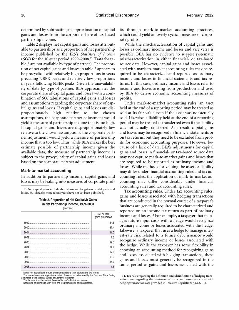
Table 2 displays net capital gains and losses attribut­able to partnerships as a proportion of net partnership income published by the IRS’s Statistics of Income (SOI) for the 10-year period 1999–2008.13 (Data for ta­ble 2 are not available by type of partner). The propor­tion of net capital gains and losses in table 2 appears to be procyclical with relatively high proportions in years preceding NBER peaks and relatively low proportions in years following NBER peaks. Given the unavailabil­ity of data by type of partner, BEA approximates the corporate share of capital gains and losses with a com­bination of SOI tabulations of capital gains and losses and assumptions regarding the corporate share of cap­ital gains and losses. If capital gains and losses are dis­proportionately high relative to the chosen assumptions, the corporate partner adjustment would yield a measure of partnership income that is too high. If capital gains and losses are disproportionately low relative to the chosen assumptions, the corporate part­ner adjustment would yield a measure of partnership income that is too low. Thus, while BEA makes the best estimate possible of partnership income given the available data, the measure of partnership income is subject to the procyclicality of capital gains and losses based on the corporate partner adjustment.

Mark-to-market accounting

In addition to partnership income, capital gains and losses may be leaking into measures of corporate prof­

13. Net capital gains include short-term and long-term capital gains and losses. SOI data for more recent years have not yet been published.

Table 2. Proportion of Net Capitalvb Gains in Net Partnership Income, 1999–2008

[Percent]

Net capital gains proportion

1999........................................................................................... 34.6

2000........................................................................................... 37.4

2001........................................................................................... 11.0

2002........................................................................................... 1.6

2003........................................................................................... 19.3

2004........................................................................................... 34.9

2005........................................................................................... 37.0

2006........................................................................................... 39.3

2007........................................................................................... 46.7

2008........................................................................................... 1.6

NOTES. Net capital gains include short-term and long-term capital gains and losses. The Shaded areas are approximate dates of recessions determined by the Business Cycle Dating

Committee of the National Bureau of Economic Research. The data are from the Internal Revenue Service’s Statistics of Income. Net capital gains include short-term and long-term capital gains and losses.

its through mark-to-market accounting practices, which could yield an overly cyclical measure of corpo­rate profits.

While the mischaracterization of capital gains and losses as ordinary income and losses and vice versa is possible, BEA has no evidence to suggest systematic mischaracterization in either financial- or tax-based source data. However, capital gains and losses associ­ated with mark-to-market accounting rules may be re­quired to be characterized and reported as ordinary income and losses in financial statements and tax re­turns. In this case, ordinary income and losses refer to income and losses arising from production and used by BEA to derive economic accounting measures of profits.

Under mark-to-market accounting rules, an asset held at the end of a reporting period may be treated as sold at its fair value even if the asset was not actually sold. Likewise, a liability held at the end of a reporting period may be treated as transferred even if the liability was not actually transferred. As a result, capital gains and losses may be recognized in financial statements or on tax returns, but they need to be excluded from prof­its for economic accounting purposes. However, be­cause of a lack of data, BEA’s adjustments for capital gains and losses in financial- or tax-based source data may not capture mark-to-market gains and losses that are required to be reported as ordinary income and losses. While methods for valuing the asset or liability may differ under financial accounting rules and tax ac­counting rules, the application of mark-to-market ac­counting may differ considerably under financial accounting rules and tax accounting rules.

Tax accounting rules. Under tax accounting rules, gains and losses associated with hedging transactions that are conducted in the normal course of a taxpayer’s business are generally required to be characterized and reported on an income tax return as part of ordinary income and losses.14 For example, a taxpayer that man­ages future input costs with a hedge would recognize ordinary income or losses associated with the hedge. Likewise, a taxpayer that uses a hedge to manage inter-est-rate risk related to a future debt issuance would recognize ordinary income or losses associated with the hedge. While the taxpayer has some flexibility in choosing an accounting method for recognizing gains and losses associated with hedging transactions, these gains and losses must generally be recognized in the same period as gains and losses associated with the

14. Tax rules regarding the definition and identification of hedging trans­actions and regarding the treatment of gains and losses associated with hedging transactions are provided in Treasury Regulations §1.1221–2.

17 February 2012 SURVEY OF CURRENT BUSINESS

underlying asset or liability.15 In cases where a hedge and the underlying asset or liability are both disposed of in the same year, recognizing the gains and losses may satisfy the recognition requirement. However, a hedging transaction may also be accounted for under mark-to-market accounting in order to satisfy the rec­ognition requirement, which results in capital gains and losses recognized on the taxpayer’s income tax re­turn as ordinary income and losses. No separate line item is required on the tax return for the gains and losses associated with the mark-to-market accounting. Thus, BEA’s adjustments to tax-based source data for capital gains and losses does not account for mark-to­market gains and losses associated with hedging trans­actions.

IRS schedule M–3 is a recent information form that corporations with $10 million or more in assets are re­quired to file. Schedule M–3 provides previously un­available details regarding receipts and deductions reported on a corporate income tax return; one of the line items on schedule M–3 is for hedging transactions. SOI has recently published tabulations of schedule M–3 for 2008, showing a hedging transactions loss of $95.1 billion. Assuming hedging transactions include some mark-to-market gains and losses, not adjusting for the mark-to-market gains and losses could yield an overly cyclical annual measure of profits and income and contribute to the statistical discrepancy. However, without more data and further study, BEA has no di­rect evidence regarding the degree or cyclicality of the mark-to-market gains and losses included in hedging transactions.

Financial accounting rules. Under financial ac­counting rules, mark-to-market accounting is required on a recurring basis (that is, periodically) for some fi­nancial assets and liabilities and may be elected for other financial assets and liabilities. Examples of finan­cial assets and liabilities include investment securities, derivative instruments, loans and other receivables, notes and other payables, and debt instruments issued. Nonfinancial assets and liabilities are generally ac­counted for at historic cost with fair value gains or losses recognized as ordinary gains or losses only when the value of an asset or liability is considered to be “other-than-temporarily” impaired. Since gains or losses associated with other-than-temporary impair­ment are only recognized on a nonrecurring basis, nonfinancial assets and liabilities are outside the cur­rent scope. Thus, the focus here is on financial ac­

15. Tax rules regarding the accounting methods for hedging transactions and regarding the recognition of gains and losses associated with hedging transactions are provided in Treasury Regulations §1.446–4 for most tax­payers except securities dealers. Accounting methods for securities dealers are provided in Treasury Regulations §1.475.

counting rules that require or allow mark-to-market accounting for financial assets and liabilities.16

Financial accounting rules distinguish three classes of debt and equity investment securities: (1) debt secu­rities intended to be held to maturity, (2) debt and eq­uity securities bought primarily for short-term trading purposes, and (3) debt and equity securities that are available for sale but not classified in the previous two classes.17 Held-to-maturity securities are accounted for at historic cost. Mark-to-market accounting is re­quired on a recurring basis for the second of the three classes—trading securities—and the third class—avail­able-for-sale securities. Trading securities include mortgage-backed securities that are held for sale in conjunction with mortgage banking activities. Mark­to-market gains and losses generated by trading securi­ties are required under financial accounting rules to be included with earnings in the income statement (that is, ordinary income or losses) with a separate disclo­sure of the amount in the notes to the financial state­ments. No separate line item is required in the financial statements for the gains and losses associated with the mark-to-market accounting. Mark-to-mar­ket gains and losses generated by available-for-sale se­curities are required to be included directly in shareholder’s equity rather than in earnings. Thus, earnings reported in financial statements may include capital gains and losses associated with trading securi­ties but not available-for-sale securities.

Financial accounting rules also require mark-to­market accounting on a recurring basis for derivative assets and liabilities, including derivatives that qualify as hedges.18 Mark-to-market gains and losses generated by derivative assets and liabilities and derivatives quali­fied as hedges of changes in fair value of an asset or lia­bility are required to be included with earnings in the income statement (that is, ordinary income or losses) with no separate line item to distinguish the mark-to­market gains or losses. In the aggregate, gains or losses associated with derivative assets should be offset by gains or losses associated with derivative liabilities. However, earnings available in disaggregated source data may include capital gains and losses associated with derivative instruments. Likewise, gains or losses associated with hedged assets or liabilities are presum­ably offset only to the extent of the gains or losses on the qualified derivative. Thus, earnings reported in fi­nancial statements may include capital gains and losses

16. Financial accounting rules for fair value measurement are provided in Statement of Financial Accounting Standards (SFAS) number 157 or topic 820 in the new Accounting Standards Codification (ASC).

17. Financial accounting rules for investments in debt and equity securi­ties are provided in SFAS number 115 or ASC topic 320.

18. Financial accounting rules for derivative instruments and hedging activities are provided in SFAS number 133 or ASC topic 815.

18 Statistical Discrepancy February 2012

associated with derivative instruments and financial assets and liabilities that have not been offset by hedges.

In addition to requiring mark-to-market account­ing for investment securities and derivative instru­ments, financial accounting rules allow companies to elect mark-to-market accounting for other financial assets and liabilities, such as receivables, payables, and debt instruments.19 A mark-to-market election is gen­erally applied to an individual instrument and is irre­vocable. In addition, similar to trading securities and derivative instruments, mark-to-market gains and losses associated with an election are required to be in­cluded with earnings in the income statement (that is, ordinary income or losses) with no separate line item. The mark-to-market election has been broadly avail­able since 2008, so earnings reported in recent finan­cial statements may include capital gains and losses associated with the financial assets and liabilities cov­ered by the accounting rules.

BEA uses financial-based source data for quarterly indicators of corporate profits in some industries. In particular, BEA uses quarterly financial reports (QFRs) provided by the Census Bureau for mining, manufac­turing, wholesale trade, and retail trade industries. QFRs include a sample of publicly owned and privately owned companies and also include adjustments to re­move capital gains and losses for use in the NIPAs. In addition to QFRs, BEA uses Compustat data for some utilities, transportation, information, real estate, and finance and insurance industries. For the finance and insurance industries, quarterly indicators come from Compustat for nondeposit credit intermediaries, secu­rities dealers, life insurance, and real estate investment trusts. The Compustat database only includes publicly owned companies and does not provide a variable to distinguish mark-to-market gains and losses included in earnings. Thus, for quarters with substantial changes in market values of securities, BEA can only resort to a small sample of quarterly financial reports filed with the Securities and Exchange Commission by individual companies to adjust for mark-to-market gains and losses.20 Assuming mark-to-market gains and losses are procyclical, overadjusting based on the chosen sample would yield a quarterly measure of profits that is not cyclical enough, and underadjusting based on the chosen sample would yield a quarterly measure of profits that is too cyclical.

19. Financial accounting rules for the fair value option for financial assets and liabilities are provided in SFAS number 159 or ASC topic 825.

20. For more information on corporate profits in the NIPAs, see Hodge (2011) and Bureau of Economic Analysis (2002).

Finance and insurance industries. Given the inclu­sion of mortgage-backed securities with trading secu­rities and given the concentration of debt and equity securities purchased and sold for finance-related activ­ities, financial institutions are particularly affected by mark-to-market accounting. Financial accounting rules for mark-to-market accounting have been under increasing scrutiny since the most recent recession (fourth quarter of 2007 to the second quarter of 2009) and the related subprime mortgage crisis because of the volatile impact that the rules have on earnings dur­ing times of market volatility. For NIPA purposes, the removal of mark-to-market gains and losses was par­ticularly important but challenging in the finance and insurance industries leading up to and following the NBER peak in the fourth quarter of 2007 because of the lack of adequate data on mark-to-market gains and losses included in earnings reported in financial state­ments and compiled in the Compustat database. Thus, declines in profits in the finance and insurance indus­tries may reflect mark-to-market losses to the extent that the losses were not identified. If so, profits in the finance and insurance industries would be under­stated.

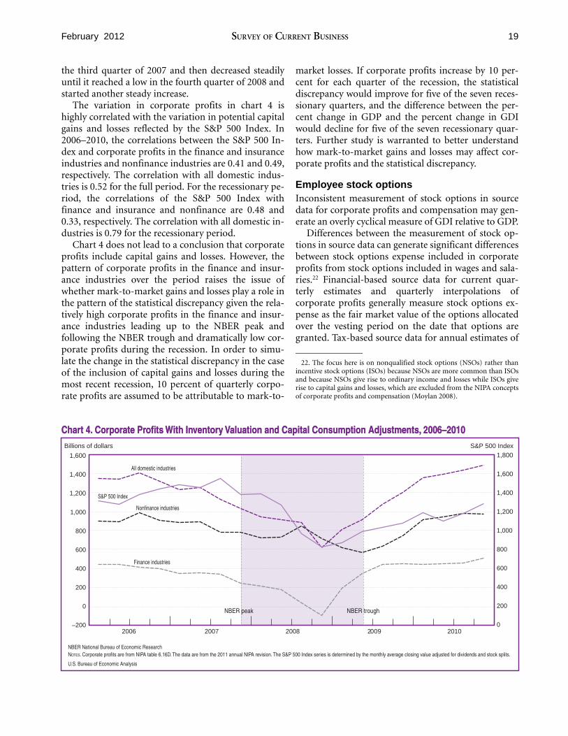
Chart 4 presents quarterly estimates of corporate profits with inventory valuation adjustment (IVA) and capital consumption adjustment (CCAdj) published in the NIPAs. Separate series are shown for the finance and insurance industries and all other industries. In addition, the chart includes a series that combines all domestic industries and, for reference to patterns of potential capital gains and losses, the chart includes a series for the S&P 500 Index measured on the right axis.21

As shown in chart 4, measured corporate profits with IVA and CCAdj generally dropped consistently from one quarter to the next for all domestic industries leading up to the NBER peak. The series for all domes­tic industries continued to decline during the reces­sion, but the decline was driven primarily by the finance and insurance industries, which dropped con­siderably more than the nonfinance industries. In ad­dition, in quarters outside of the recession, corporate profits in the finance and insurance industries were generally as high as at least 40 percent of corporate profits in nonfinance industries; however, during the recession, corporate profits in the finance and insur­ance industries dropped to less than 5 percent of cor­porate profits in nonfinance industries for some quarters. The S&P 500 Index increased steadily until

21. The S&P 500 Index series is determined by the monthly average clos­ing value adjusted for dividends and stock splits.

19

Billions of dollars S&P 500 Index

1,600 1,800

All domestic industries 1,400 1,600

1,200 S&P 500 Index 1,400

1,000 Nonfinance industries 1,200

800 1,000

600 800

Finance industries 400 600

200 400

0 NBER peak NBER trough

200

–200 2006 2007 2008 2009

0 2010

NBER National Bureau of Economic Research

February 2012 SURVEY OF CURRENT BUSINESS

CharChartt 4.4. Corporate PrCorporate Profitsofits With InWith Inventorventoryy VVaaluation and Capital Consumption Adjustments,luation and Capital Consumption Adjustments, 2006–20102006–2010

NOTES. Corporate profits are from NIPA table 6.16D. The data are from the 2011 annual NIPA revision. The S&P 500 Index series is determined by the monthly average closing value adjusted for dividends and stock splits.

U.S. Bureau of Economic Analysis

the third quarter of 2007 and then decreased steadily until it reached a low in the fourth quarter of 2008 and started another steady increase.

The variation in corporate profits in chart 4 is highly correlated with the variation in potential capital gains and losses reflected by the S&P 500 Index. In 2006–2010, the correlations between the S&P 500 In­dex and corporate profits in the finance and insurance industries and nonfinance industries are 0.41 and 0.49, respectively. The correlation with all domestic indus­tries is 0.52 for the full period. For the recessionary pe­riod, the correlations of the S&P 500 Index with finance and insurance and nonfinance are 0.48 and 0.33, respectively. The correlation with all domestic in­dustries is 0.79 for the recessionary period.

Chart 4 does not lead to a conclusion that corporate profits include capital gains and losses. However, the pattern of corporate profits in the finance and insur­ance industries over the period raises the issue of whether mark-to-market gains and losses play a role in the pattern of the statistical discrepancy given the rela­tively high corporate profits in the finance and insur­ance industries leading up to the NBER peak and following the NBER trough and dramatically low cor­porate profits during the recession. In order to simu­late the change in the statistical discrepancy in the case of the inclusion of capital gains and losses during the most recent recession, 10 percent of quarterly corpo­rate profits are assumed to be attributable to mark-to­

market losses. If corporate profits increase by 10 per­cent for each quarter of the recession, the statistical discrepancy would improve for five of the seven reces­sionary quarters, and the difference between the per­cent change in GDP and the percent change in GDI would decline for five of the seven recessionary quar­ters. Further study is warranted to better understand how mark-to-market gains and losses may affect cor­porate profits and the statistical discrepancy.

Employee stock options Inconsistent measurement of stock options in source data for corporate profits and compensation may gen­erate an overly cyclical measure of GDI relative to GDP.

Differences between the measurement of stock op­tions in source data can generate significant differences between stock options expense included in corporate profits from stock options included in wages and sala­ries.22 Financial-based source data for current quar­terly estimates and quarterly interpolations of corporate profits generally measure stock options ex­pense as the fair market value of the options allocated over the vesting period on the date that options are granted. Tax-based source data for annual estimates of

22. The focus here is on nonqualified stock options (NSOs) rather than incentive stock options (ISOs) because NSOs are more common than ISOs and because NSOs give rise to ordinary income and losses while ISOs give rise to capital gains and losses, which are excluded from the NIPA concepts of corporate profits and compensation (Moylan 2008).

20 Statistical Discrepancy February 2012

corporate profits generally measure this expense as the difference between the market price of the stock and the strike price of the options on the date that the op­tions are exercised. Source data for wages and salaries estimates initially come from the Current Employment Statistics (CES) program at the Bureau of Labor Statis­tics (BLS). The CES data exclude income from stock options. Five months after the reference quarter, BEA incorporates data into wage and salary estimates from the BLS’s Quarterly Census of Employment and Wages (QCEW). The QCEW includes income from stock op­tions measured consistently with the annual tax-based source data.

Given the consistent measurement of stock options in the annual tax-based source data underlying corpo­rate profits and the QCEW data underlying wages and salaries estimates, the measurement and timing differ­ences should not affect the annual statistical discrep­ancy by the second annual revision because QCEW data and tax-based source data are fully incorporated into the NIPAs by then. However, the measurement and timing differences are likely to contribute to the statistical discrepancy in current quarterly estimates, and the effect is likely to persist in the quarterly inter­polations after the first annual revision because stock options are measured inconsistently in quarterly finan­cial-based source data and in the QCEW. The procycli­cal nature of stock prices and the incentive for employees to exercise stock options when stock prices increase as well as the disincentive when stock prices decrease may yield an overly cyclical measure of quar­terly wages and salaries. In contrast, quarterly corpo­rate profits as measured by financial-based source data would be less affected by changes in stock prices be­cause stock options expenses in quarterly financial data is measured when stock options are granted and are distributed evenly over the vesting period. Thus, GDI may be overstated relative to GDP during stock market increases but understated during stock market declines. Moylan (2008) provides a comprehensive dis­cussion regarding the inclusion of stock options in measures of corporate profits and compensation.

Produced intangibles Any error in assumptions regarding the capitalization rate of produced intangibles results in inaccurate mea­sures of profits and income.

In the year that produced intangibles are acquired, the seller of the intangibles recognizes revenue and the buyer recognizes expense for tax purposes if intangi­bles are not capitalized and depreciated. In this case, revenues offset expenses, and the statistical discrep­

ancy is unaffected. When produced intangibles are capitalized and depreciated for tax purposes, BEA adds the depreciation back to tax-based receipts less deduc­tions, which is the starting point for profits and in­come, and includes the depreciation in consumption of fixed capital, which is BEA’s measure of depreciation included in GDI.

In the case of purchased computer software, BEA assumes a low rate of capitalization for tax purposes.23

As a result, the depreciation for produced intangibles that is added back to tax-based receipts less deductions includes only a small amount of depreciation for soft­ware. In the year software is purchased, tax-based re­ceipts less deductions overstates profits and income to the extent that software is capitalized and not depreci­ated for tax purposes beyond BEA’s assumed rate of capitalization (that is, when aggregate receipts from software sales are greater than aggregate deductions from software purchases). Thus, the statistical discrep­ancy may be affected. In the years that software is de­preciated, the statistical discrepancy is unaffected because the capital consumption adjustment absorbs the difference between the actual depreciation and the assumed depreciation. Assuming software purchases are procyclical, failure to accurately adjust for capital­ized software would yield a measure of profits and in­come that may be too high during cyclical upturns but less affected during downturns.

Summary and Conclusions This article explains the significant role that profits and income play in BEA’s decision to record the statis­tical discrepancy as a separate line item on the income side of the NIPAs and an overview of the factors of profits and income that are most likely contributing to the statistical discrepancy.

BEA’s decision to record the statistical discrepancy with GDI reflects BEA’s experience and careful consid­eration of the reliability of the underlying source data. Source data underlying GDP are generally consistent with economic accounting concepts and thus consid­ered more reliable than source data underlying GDI. In contrast, data underlying the profits and income com­ponents of GDI are generally collected from financial-and tax-based sources, which can be inconsistent with economic accounting concepts and thus require ad­justments for economic accounting purposes. While BEA works to reduce measurement error related to the

23. U.S. tax law allows taxpayers to deduct the cost in the year of acquisi­tion rather than to capitalize and depreciate the cost of qualifying property, including purchased computer software, subject to deduction limitations and other restrictions.

21 February 2012 SURVEY OF CURRENT BUSINESS

source data and required adjustments, the work is lim­ited by conceptual differences and regulatory reporting requirements underlying the financial- and tax-based source data.

This article specifically discussed four factors that require adjustments to convert financial- or tax-based source data into economic accounting measures of profits and income. First, adjustments for misreport­ing are likely factors contributing to the statistical dis­crepancy, and the direction of the effect is ambiguous without further study. Second, capital gains and losses may be leaking into measures of profits and income and contributing to the statistical discrepancy through corporate partner adjustments and mark-to-market accounting practices, which could yield overly cyclical measures of profits and income. Measurement of prof­its in the finance and insurance industries was particu­larly challenging during the most recent recession. Third, inconsistent measurement of stock options in source data for corporate profits and wages and sala­ries may generate an overly cyclical measure of GDI relative to GDP. Finally, any error in assumptions re­garding the capitalization rate of purchased software may overstate profits and income during cyclical up­turns.

These issues lend support to BEA’s practices of not promoting one output measure over another and of recording the statistical discrepancy in a transparent manner on the income side of the NIPAs. However, more attention should be given to describing the GDI estimates in a manner that will inform the public about this alternative source of macroeconomic infor­mation. Furthermore, additional research is warranted on factors contributing to the statistical discrepancy, on a framework for weighting underlying source data in an effort to distribute the statistical discrepancy, and on a framework and appropriate weights for a com­bined output measure.

References Bureau of Economic Analysis. 2002. Corporate Profits: Profits Before Tax, Profits Tax Liability, and Dividends. Methodology Paper. Washington, DC: Bureau of Eco­nomic Analysis, September; www.bea.gov/scb/pdf/ national/nipa/methpap/methpap2.pdf.

Byron, Ray P. 1978. “The Estimation of Large Social Account Matrices.” Journal of the Royal Statistical Soci­ety, Series A 141, part 3 (March): 359–367.

Chen, Baoline. 2006. “A Balanced System of Indus­try Accounts for the U.S. and Structural Distribution of Statistical Discrepancy.” BEA Working Paper WP2006–8. Washington, DC: Bureau of Economic Analysis; www.bea.gov.

Chen, Baoline. 2010. “Reconciling the System of

U.S. Accounts and Distribution of the Aggregate Statis­tical Discrepancy.” Unpublished. Washington, DC: Bu­reau of Economic Analysis.

European Commission, International Monetary Fund, Organisation for Economic Co-operation and Development, United Nations, and World Bank. 2009. System of National Accounts 2008. New York: United Nations.

Financial Accounting Foundation, Financial Ac­counting Standards Board. Statement of Financial Ac­counting Standards. Numbers 115 (May 1993), 133 (June 1998), 157 (September 2006), and 159 (February 2007).

Financial Accounting Foundation, Financial Ac­counting Standards Board. Accounting Standards Codi­fication. Topics 320, 815, 820, and 825.

Fixler, Dennis J., and Bruce T. Grimm. 2002. “Reli­ability of GDP and Related NIPA Estimates.” SURVEY OF

CURRENT BUSINESS 81 (January): 9–27. Fixler, Dennis J., and Bruce T. Grimm. 2005. “Reli­

ability of the NIPA Estimates of U.S. Economic Activ­ity.” SURVEY OF CURRENT BUSINESS 85 (February): 8–19.

Fixler, Dennis J., and Jeremy J. Nalewaik. 2009. “News, Noise, and Estimates of the “True” Unobserved State of the Economy.” BEA Working Paper WP2010– 04. Washington, DC: Bureau of Economic Analysis; www.bea.gov.

Fixler, Dennis J., Ryan Greenaway-McGrevy, and Bruce T. Grimm. 2011. “Revisions to GDP, GDI, and Their Major Components.” SURVEY OF CURRENT BUSINESS

91 (July): 9–31. Greenaway-McGrevy, Ryan. 2011. “Is GDP or GDI a

Better Measure of Output? A Statistical Approach.” BEA Working Paper WP2011–08. Washington, DC: Bureau of Economic Analysis; www.bea.gov.

Grimm, Bruce T. 2007. “The Statistical Discrep­ancy.” BEA Working Paper WP2007–01. Washington, DC: Bureau of Economic Analysis; www.bea.gov.

Grimm, Bruce T., and Robert P. Parker. 1998. “Reli­ability of the Quarterly and Annual Estimates of GDP and Gross Domestic Income.” SURVEY OF CURRENT BUSI­NESS 78 (December): 12–21.

Grimm, Bruce T., and Teresa L. Weadock. 2006. “Gross Domestic Product: Revisions and Source Data.” SURVEY OF CURRENT BUSINESS 86 (February): 11–15.

Holdren, Alyssa E., and Bruce T. Grimm. 2008. “Gross Domestic Income: Revisions and Source Data.” SURVEY OF CURRENT BUSINESS 88 (December): 14–20.

Hodge, Andrew W. 2011. “Comparing NIPA Profits With S&P 500 Profits.” SURVEY OF CURRENT BUSINESS 91 (March): 22–27.

Internal Revenue Service, U.S. Department of the Treasury. Code of Federal Regulations, Title 26. “Chapter I, Subchapter A, Part 1, sections 446, 475,

22 Statistical Discrepancy February 2012

and 1221.” Washington, DC: Internal Revenue Service. Klein, Lawrence R., and J. Junichi Makino. 2000.

“Economic Interpretations of the Statistical Discrep­ancy.” Journal of Economic and Social Measurement 26 (January), no. 1, 11–29.

Landefeld, J. Steven. 2010. “Comments on ‘The In­come- and Expenditure-Side Estimates of U.S. Output Growth.” Brookings Papers on Economic Activity 1 (Spring): 112–123.

Mankiw, N. Gregory, and Matthew D. Shapiro. 1986. “News or Noise: An Analysis of GNP Revisions.” SURVEY OF CURRENT BUSINESS 66 (May): 20–25.

Moylan, Carol E. 2008. “Employee Stock Options and the National Economic Accounts.” SURVEY OF CUR­RENT BUSINESS 88 (February): 7–13.

Nalewaik, Jeremy J. 2010. “The Income- and Expen­diture-Side Estimates of U.S. Output Growth.” Brook­ings Papers on Economic Activity 1 (Spring): 71–106.

Rassier, Dylan G., Thomas F. Howells III, Edward T.

Morgan, Nicholas R. Empey, and Conrad E. Roesch. 2007. “Implementing a Reconciliation and Balancing Model in the U.S. Industry Accounts.” BEA Working Paper WP2007–05. Washington, DC: Bureau of Eco­nomic Analysis; www.bea.gov.

Smith, Richard J., Martin R. Weale, and Steven E. Satchell. 1998. “Measurement Error with Accounting Constraints: Point and Interval Estimation for Latent Data with an Application to U.K. Gross Domestic Product.” The Review of Economic Studies 65, no. 1 (January): 109–134.

Stone, Richard, James E. Meade, and David G. Champernowne. 1942. “The Precision of National In­come Estimates.” The Review of Economic Studies 9, no. 2 (Summer): 111–125.

Weale, Martin. 1992. “Estimation of Data Measured with Error and Subject to Linear Restrictions.” Journal of Applied Econometrics 7, no. 2 (April–June): 167–174.