the role of politics and instability on public …etd.lib.metu.edu.tr/upload/12604711/index.pdf ·...

THE ROLE OF POLITICS AND INSTABILITY ON PUBLICSPENDING DYNAMICS AND MACROECONOMIC PERFORMANCE:

THEORY AND EVIDENCE FROM TURKEY

A THESIS SUBMITTED TOTHE GRADUATE SCHOOL OF SOCIAL SCIENCES

OFMIDDLE EAST TECHNICAL UNIVERSITY

BY

MUSTAFA İSMİHAN

IN PARTIAL FULFILLMENT OF THE REQUIREMENTS FOR THE DEGREE OF

DOCTOR OF PHILOSOPHY

IN

THE DEPARTMENT OF ECONOMICS

DECEMBER 2003

Approval of the Graduate School of Social Sciences

___________________________

Prof. Dr. Sencer AYATA

Director

I certify that this thesis satisfies all the requirements as a thesis for the degree of Doctor of

Philosophy.

___________________________

Prof. Dr. Erol ÇAKMAK

Head of Department

This is to certify that we have read this thesis and that in our opinion it is fully adequate, in

scope and quality, as a thesis for the degree of Doctor of Philosophy.

____________________________ ____________________________

Assoc. Prof. Dr. Kõvõlcõm Prof. Dr. Aysõt TANSEL

METİN-ÖZCAN Supervisor

Co-Supervisor

Examining Committee Members

Prof. Dr. Aysõt TANSEL ___________________________

Assoc. Prof. Dr. Kõvõlcõm METİN-ÖZCAN ___________________________

Prof. Dr. Merih CELASUN ___________________________

Assoc. Prof. Dr. Nazõm EKİNCİ ___________________________

Dr. Elif AKBOSTANCI ___________________________

iii

ABSTRACT

THE ROLE OF POLITICS AND INSTABILITY ON PUBLIC

SPENDING DYNAMICS AND MACROECONOMIC PERFORMANCE:

THEORY AND EVIDENCE FROM TURKEY

İsmihan, Mustafa

Ph.D., Department of Economics

Supervisor: Prof. Dr. Aysõt Tansel

Co-Supervisor: Assoc. Prof. Dr. Kõvõlcõm Metin-Özcan

December 2003, 244 pages

This Ph.D. thesis comprises of two parts. Part I develops a framework to provide

insights into the understanding of several political macro-economy issues related

to fiscal policy making. This framework links the overall macroeconomic

performance to the public spending and borrowing decisions. The key feature of

this framework is that it makes a distinction between productive (e.g. public

investment) and non-productive public spending (e.g. popular spending). It is

shown that a high level of political instability may lead to myopic and populist

policies and may be associated with less favorable macroeconomic performance

in terms of not only future output and inflation but also future popular spending.

iv

Part I also suggests an alternative channel for expansionary or Non-Keynesian

fiscal contractions based on the productivity enhancing role of productive public

spending. It is shown that if the incumbent government reduces popular

(productive) spending rather than productive (popular) spending, then Non-

Keynesian (Keynesian) effects are achieved. Furthermore, it is shown that the

favorable effects of public investment depends positively on its quality in this

framework. Moreover, the net effect of productive spending financed by

borrowing on the next period's macroeconomic performance depends on the

benefits of productive spending relative to the costs of borrowing. Even under a

capital borrowing rule higher public investment may yield unfavorable effects and

also it may not necessarily prevent the strategic use of public investment, even

though it prevents strategic debt accumulation. Part II investigates the effects of

macroeconomic instability on capital accumulation and economic growth in the

Turkish economy over the 1963-1999 period. Descriptive and econometric (time

series) analyses suggest that macroeconomic instability not only deters capital

accumulation and economic growth but it may also reverse the complementarity

between public and private investment in the long-run.

Keywords: Composition of Public spending; Political Instability; Macroeconomic

Performance; Strategic Debt Accumulation; Capital Borrowing Rule; Public

Investment; Private Investment; Complementarity; Macroeconomic Instability.

v

ÖZ

SİYASET VE İSTİKRARSIZLIĞIN KAMU HARCAMA DİNAMİKLERİ

VE MAKROEKONOMİK PERFORMANS ÜZERİNDEKİ ROLÜ:

TEORİ VE TÜRKİYE DENEYİMİ

İsmihan, Mustafa

Doktora, Ekonomi Bölümü

Tez Yöneticisi: Prof. Dr. Aysõt Tansel

Ortak Tez Yöneticisi: Doç. Dr. Kõvõlcõm Metin-Özcan

Aralõk 2003, 244 sayfa

Bu doktora tezi iki kõsõmdan oluşmaktadõr. Birinci kõsõm maliye politikalarõnõn

oluşturulmasõ ile ilgili bazõ politik makro-iktisat konularõnõn daha iyi anlaşõlmasõ

için teorik bir çerçeve oluşturmaktadõr. Bu kurguda makroekonomik performans

ile kamu harcama ve borçlanma kararlarõ ilişkilendirilmektedir. Bu kurgunun

temel özelliği verimli (örneğin kamu yatõrõmlarõ) ve verimsiz kamu harcamalarõ

(örneğin popüler harcamalar) arasõnda bir ayõrõmõn yapõlmasõdõr. Yüksek düzeyde

siyasi istikrarsõzlõğõn kõsa görüşlü ve popülist politikalara ve dolayõsõyla daha kötü

bir makroekonomik performansa yol açabileceği, ve bunun sadece gelecekteki

üretim ve enflasyon açõsõndan değil aynõ zamanda gelecekteki popüler harcamalar

vi

açõsõndan da kötü olabileceği gösterilmiştir. Ayrõca, birinci kõsõmda, verimli kamu

harcamalarõnõn verimliliği artõrõcõ rolü dikkate alõnarak, genişletici veya

Keynesyen olmayan mali daralmalar için alternatif bir kanal önerilmektedir.

Hükümetin popüler (verimli) harcamalar yerine verimli (popüler) harcamalarõ

azaltmasõ halinde Keynesyen (Keynesyen olmayan), yani daraltõcõ (genişletici) bir

etkinin gerçekleştiği gösterilmiştir. Buna ilaveten, bu çerçevede kamu

yatõrõmlarõnõn kalitesinin de kamu yatõrõmlarõnõn olumlu etkilerini pozitif yönde

etkilediği gösterilmiştir. Bunlarõn yanõ sõra, borçlanma ile finanse edilen verimli

harcamalarõn gelecek dönemdeki makroekonomik performans üzerindeki net

etkileri bu harcamalarõn olumlu etkilerinin yanõ sõra borçlanmanõn maliyetinede

bağlõdõr. Sermaye borçlanma kuralõnõn uygulanmasõ, başka bir deyişle yatõrõm için

borçlanma durumunda dahi kamu yatõrõmlarõndaki bir artõşõn makroekonomik

performans üzerinde olumsuz etkileri olabilir ve bu kuralõn uygulanmasõ her ne

kadar stratejik amaçlõ borçlanmayõ engellese de, kamu yatõrõmlarõnõn stratejik

amaçlõ kullanõmõnõ engellemeyebilir. İkinci kõsõm Türkiye ekonomisindeki

makroekonomik istikrarsõzlõğõn sermaye birikimi ve ekonomik büyüme üzerindeki

etkilerini 1963-1999 yõllarõ için araştõrmaktadõr. Tasviri ve ekonometrik (zaman

serisi) analizler makroekonomik istikrarsõzlõğõn sermaye birikimini ve ekonomik

büyümeyi kötü etkilemekle kalmayõp ayrõca uzun vadede kamu yatõrõmlarõ ve özel

yatõrõmlar arasõndaki tamamlayõcõlõk ilişkisini tersine çevirmiş olabileceğini

göstermiştir.

Anahtar kelimeler: Kamu Harcamalarõnõn Bileşimi; Politik İstikrarsõzlõk;

Makroekonomik Performans; Stratejik Borç Birikimi; Sermaye Borçlanma Kuralõ;

Kamu Yatõrõmlarõ; Özel Yatõrõmlar; Tamamlayõcõlõk; Makroekonomik

İstikrarsõzlõk.

vii

To my parents and my wife

viii

Bu tez Türkiye Bilimler Akademisi Sosyal Bilimlerde Yurtiçi - YurtdõşõBütünleştirilmiş Doktora Burs Programõ tarafõndan desteklenmiştir.

This thesis has received the financial support of the Turkish Academy of SciencesFellowship Programme for Integrated Doctoral Studies in Turkey

and/or Abroad in the Social Sciences and Humanities.

ix

ACKNOWLEDGEMENTS

I would like to thank my thesis supervisors Prof. Dr. Aysõt Tansel, Assoc. Prof.

Dr. Kõvõlcõm Metin-Özcan and Dr. F. Gülçin Özkan for their excellent

supervision, invaluable guidance and support throughout this research.

I am also very grateful to the members of the thesis committee Prof. Dr. Merih

Celasun and Assoc. Prof. Dr. Nazõm Ekinci for their insight, helpful comments

and suggestions. My thanks also go to the examining committee member Dr. Elif

Akbostancõ for her helpful comments and suggestions. I would especially like to

thank Asst. Prof. Dr. Özge Şenay for her support, helpful comments, suggestions

and careful proofreading.

The theoretical part (Part I) of this thesis was written during my stay at the

University of York as a visiting scholar, I would like to thank the Department of

Economics and Related Studies (DERS) for their hospitality and to the Turkish

Academy of Sciences (TÜBA) for their financial support which has made this

visit possible.

Also, I would like to thank all of my professors at METU for the new dimensions

and perspective that they have given me during my Ph.D. study. Especially, I

would like to thank Prof. Dr. Fikret Şenses for the encouragement, support and

motivation that have helped me throughout my Ph.D. study at METU. Also, my

sincere thanks go to Prof. Dr. Fikret Görün for his support and encouragement.

x

I appreciate the helpful comments and/or suggestions of Prof. Dr. Karim Abadir

and Prof. Dr. Katarina Juselius in some econometric issues. Also, I would like to

thank Prof. Dr. Oktar Türel, Assoc. Prof. Dr. Cem Somel, Asst. Prof. Dr. Şirin

Saraçoğlu, Nil Demet Güngör and others that I have forgotten to mention by name

for their valuable help on various issues.

Last but not least I would like to thank my wife Fatma for her great help,

encouragement and support at every stage of my Ph.D. study. Also I would like to

thank my parents for their encouragement, support and love that have made it

easier for me to concentrate on my studies.

xi

TABLE OF CONTENTS

ABSTRACT .. iii

ÖZ . v

ACKNOWLEDGEMENTS .. ix

TABLE OF CONTENTS .. xi

LIST OF TABLES xvi

LIST OF FIGURES ... xviii

CHAPTER1. INTRODUCTION AND OVERVIEW 1

1.1 Part I: Politics, Public Spending, Borrowing andMacroeconomic Performance 3

1.1.1 Introduction to Part I .. 3

1.1.2 An Overview of Part I 9

1.2 Part II: Macroeconomic Instability, Capital Accumulation andEconomic Growth: The Turkish Experience 1963-1999 ... 12

1.2.1 Introduction to Part II .... 121.2.2 An Overview of Part II .. 15

Part I: Politics, Public Spending, Borrowing and MacroeconomicPerformance

2. POLITICS, PUBLIC SPENDING, BORROWING, ANDMACROECONOMIC PERFORMANCE: A REVIEW OFRELATED LITERATURE ... 18

2.1 Introduction ... 18

xii

2.2 Public Investment, Productivity and Output: An Overview ... 20

2.3 The Role of Socio-Political Factors on Public Spending,Borrowing and Macroeconomic Performance ... 22

2.3.1 Inequality, Fractionalization, Polarization and Populism 23

2.3.2 Electoral Uncertainty, Myopia and Strategic PoliticalBehavior . 24

2.4 Corruption and Public Investment .. 31

2.5 Expansionary Fiscal Adjustment ... 32

2.6 A Road Map for the Rest of Part I .. 33

3. THE IMPACT OF PRODUCTIVE VS. NON-PRODUCTIVEPUBLIC SPENDING ON MACROECONOMICPERFORMANCE .. 35


3.2 The Benchmark Model .. 39

3.2.1 Model ..... 40

3.2.2 Features of the Equilibrium ....... 41

3.3 The Basic Dynamic Model: Extending the Benchmark Modelwith Productive Public Spending .. 44

3.3.1 Model ..... 44

3.3.2 Equilibrium Macroeconomic Outcomes 46

3.4 Decentralized Policy Making 53

3.4.1 The Decentralized Benchmark Model 53

3.4.2 The Decentralized Dynamic Model ... 56

3.5 Conclusion . 58

4. THE POLITICAL ECONOMY OF THE COMPOSITION OFPUBLIC SPENDING AND FISCAL ADJUSTMENT 61

xiii


4.2 Political Economy of the Composition of Public Spending .. 63

4.2.1 Political Instability and Polarization .. 63

4.2.2 Quality of Productive Public Spending: Corruption andFavoritism ... 70

4.3 Political Economy of Composition of Fiscal Adjustment . 72

4.5 Conclusion . 73

5. THE ROLE OF PUBLIC DEBT AND THE CAPITALBORROWING RULE ON PUBLIC SPENDING ANDMACROECONOMIC PERFORMANCE ..... 76


5.2 An Extended Model with Debt Dynamics . 79

5.2.1 Model . 80


5.2.3 Strategic Use of Debt Policy .. 86

5.3 The Double Dynamics Model: Borrowing Vs. ProductiveSpending 89

5.3.1 Model . 89


5.4 Capital Borrowing Rule . 99

5.5 Conclusion . 106

Part II: Macroeconomic Instability, Capital Accumulation andEconomic Growth: The Turkish Experience 1963-1999

6. REVIEW OF THE LITERATURE ON THE ROLE OFPUBLIC INVESTMENT AND MACROECONOMICINSTABILITY IN CAPITAL ACCUMULATION ANDECONOMIC GROWTH ... 110


xiv

6.2 The Role of Public Investment in Capital Formation andEconomic Growth .. 111

6.2.1 Public Capital Spending-Private Investment Nexus .. 112

6.2.2 Public Spending-Output (Growth) Nexus . 119

6.3 The Role of Macroeconomic Instability in CapitalAccumulation and Growth 129

6.3.1 Theoretical arguments ... 130

6.3.2 Empirical Evidence 133

6.4 Turkish Evidence: An Overview ... 135

6.5 A Road Map for the Rest of Part II ... 137

7. AN OVERVIEW OF MACROECONOMIC INSTABILITYPROCESSES, PUBLIC SPENDING, INVESTMENT ANDGROWTH DYNAMICS IN THE TURKISH ECONOMY,1963-1999 .. 138


7.2 The Inward-Oriented Period, 1963-1979 .. 140

7.3 The Outward-Oriented Period, 1980-99 149

7.4 Conclusion . 160

8. AN EMPIRICAL ANALYSIS OF THE ROLE OFMACROECONOMIC INSTABILITY IN PUBLIC ANDPRIVATE CAPITAL ACCUMULATION AND GROWTH:THE TURKISH EXPERIENCE, 1963-1999 .... 162


8.2 Methodology .. 164

8.3 Empirical Results ... 168

8.3.1 The Data and Unit Root Tests ... 168

8.3.2 Cointegration Analyses .. 171

xv

8.3.3 Impulse Response Analyses .. 176

8.4 Conclusion and Policy Implications .. 181

9. CONCLUSIONS ... 183

APPENDICESA. DERIVATION OF OUTPUT SUPPLY FUNCTION .. 189

B. DERIVATION OF THE BUDGET CONSTRAINT 190

C. DERIVATION OF THE POLICY OUTCOMES OF THEBENCHMARK MODEL .. 192

D. DERIVATION OF AUGMENTED OUTPUT SUPPLYFUNCTION .. 194

E. DERIVATION OF THE EQUILIBRIUM POLICYOUTCOMES OF THE BASIC DYNAMIC MODEL .. 196

F. DERIVATION OF THE POLICY OUTCOMES OF THEDECENTRALIZED BENCHMARK MODEL 199

G. DERIVATION OF THE EQUILIBRIUM POLICYOUTCOMES OF THE BASIC DYNAMIC MODELUNDER ELECTORAL UNCERTAINTY ... 202

H. DERIVATION OF THE NEW BUDGET CONSTRAINT .. 205

I. DERIVATION OF THE EQUILIBRIUM POLICYOUTCOMES OF AN EXTENDED BENCHMARKMODEL WITH DEBT DYNAMICS ... 206

J. DERIVATION OF THE EQUILIBRIUM POLICYOUTCOMES OF THE DOUBLE DYNAMICS MODEL 209

K. DATA APPENDIX ... 212

L. TURKISH SUMMARY ... 216

REFERENCES . 227

VITA . 244

xvi

LIST OF TABLES

TABLE3.1 Output Gap, Public Spending Gap and Inflation Rate: The

Benchmark Model ........ 43

3.2 Final-period Optimal Policy Outcomes: The Basic DynamicModel ...... 47

3.3 Equilibrium Macroeconomic Outcomes in t=1 and t=2: TheBasic Dynamic Model .... 47

3.4 Output Gap, Public Spending Gap and Inflation Rate in t=2:The Basic Dynamic Model ..... 48

3.5 Comparative Statics: The Basic Dynamic Model .. 50

3.6 Equilibrium Macroeconomic Outcomes: DecentralizedBenchmark Case 55

3.7 Equilibrium Macroeconomic Outcomes in t=1 and t=2:(Dynamic) Decentralized Case ... 57

4.1 Output Gap, Public Spending Gap and Inflation RateUnder the Presence of Corruption .. 71

5.1 Final-period Optimal Policy Outcomes: An Extended Modelwith Debt Dynamics Model ... 82

5.2 Equilibrium Macroeconomic Outcomes in t=1 and t=2: AnExtended Model with Debt Dynamics Model . 83

5.3 Output Gap, Public Spending Gap and Inflation Rate: AnExtended Model with Debt Dynamics .. 84

5.4 Comparative Statics: An Extended Model with Debt Dynamics 86

5.5 Final-period Optimal Policy Outcomes: The Double DynamicsModel ..... 91

xvii

5.6 Equilibrium Macroeconomic Outcomes in t=1: The DoubleDynamics Model ....……..……………………………………. 92

5.7 Comparative Statics in t=2: The Double Dynamics Model ..… 93

5.8 Output Gap, Public Spending Gap and Inflation Rate: TheDouble Dynamics Model ...…...………………………………. 93

5.9 Comparative Statics in t=1: The Double Dynamics Model …... 94

5.10 Output Gap, Public Spending Gap and Inflation Rate UnderCapital Borrowing Rule ………………………………………. 101

5.11 Comparative Statics in t=2 (Capital Borrowing Rule) ……….. 102

5.12 Equilibrium Macroeconomic Outcomes in t=1 Under CapitalBorrowing Rule ………………………………………………. 103

5.13 Productive Spending in t=1: Comparative Statics (CapitalBorrowing Rule) ……………………………………………… 104

7.1 Selected Indicators on the Turkish Economy, 1963-1999 ……. 142

7.2 Political Instability, Public Spending and Debt Dynamics,1980-1999 …………………………………………………….. 153

8.1 Unit Root Tests ……………………………………………….. 170

8.2 Cointegration Analysis of System #1 ………………………… 174

8.3 Cointegration Analysis of System #2 ………………………… 174

G.1 Equilibrium Macroeconomic Outcome Under ElectoralUncertainty in t=1 and t=2 ……………………………………. 204

xviii

LIST OF FIGURES

FIGURE7.1 Real GNP, 1963-1999 ... 142

7.2 Real Private Investment, 1963-1999 . 143

7.3 Real Public Investment and Its Infrastructural Component,1963-1999 .. 143

7.4 Private Investment-GNP Ratio (current), 1963-1999 146

7.5 Public Investment-GNP Ratio (current), 1963-1999 . 146

7.6 Inflation, 1963-1999 .. 147

7.7 Macroeconomic Instability Index (MII), 1963-1999 . 147

7.8 Public Infrastructural Investment (% of total publicinvestment), 1963-1999 . 153

7.9 Macroeconomic Instability Vs. Share of Public Investment inTotal Public Expenditures of Consolidated Budget, 1975-1999 159

7.10 Composition of Public Spending out of Consolidated Budget,1975-1999 .. 159

8.1 Time plot of the logarithm of real GNP (y), 1963-1999 169

8.2 Time plots of the logarithms of real fixed private investment(ip), real fixed public investment (ig) and real fixed public coreinfrastructural investment (igi), 1963-1999 ... 169

8.3 Time plot of the logarithm of macroeconomic instability index(mii), 1963-1999 170

8.4 Generalized IR(s) to one S.E. shock in the equation for mii, igand y (System #1) .. 178

xix

8.5 Generalized IR(s) to one S.E. shock in the equation for mii, igand y (System #2) .. 179

CHAPTER 1

INTRODUCTION AND OVERVIEW

The policy makers in Turkey and in many other developing countries, such

as those in Latin America, behaved Þscally irresponsible by implementing

myopic and populist macroeconomic policies over extended periods of time.

These countries, in turn, persistently exhibited high budget deÞcits, excessive

debt accumulation, high and volatile inßation rates. Hence, chronic macroeco-

nomic instability has become a central feature of their economies. Additionally,

during their macroeconomic instability episodes, most of these countries have

registered remarkable declines as well as volatility in their rates of capital for-

mation. In retrospect, continuously low and volatile economic growth rates

and recurrent crises have become an endemic feature of these economies.

Several authors argue that unsound policies, such as myopic and populist

policies, and associated macroeconomic instability of developing countries usu-

ally emanate from deeper socio-political instabilities (e.g. due to income distri-

bution) but not from technical mistakes or misjudgments of policy makers.1

Dornbusch and Edwards (1991), for instance, provide evidence on the link

1See, for example, introduction part and a number of papers collected in Sachs (1989).

1

between macroeconomic populism2 and income inequality as well as on detri-

mental consequences of populist policies on macroeconomic stability, based on

Latin American experience. The main results of this study is nicely summa-

rized in Dornbusch and Edwards (1995):3

although populist episodes have had speciÞc and unique character-

istics in different nations, they tend to have some fundamental common

threads. In particular, populist regimes have historically tried to deal

with income inequality problems through the use of overly expansive

macroeconomic policies. These policies, which have relied on deÞcit

Þnancing, generalized controls, and a disregard for basic economic prin-

ciples, have almost unavoidably resulted in major macroeconomic crises

that ended up hurting poorest segments of society. At the end of every

populist experiment, inßation is out of hand, macroeconomic disequi-

libria are ramphant, and real wages are lower than they were at the

beginning of these experiences (Dornbusch and Edwards, 1995: 5).

Likewise, many other economists nowadays emphasize both the importance

and the role of the socio-political environment on numerous economic poli-

cies, such as public spending and borrowing policies, and resultant outcomes.4

Therefore, one of the main objectives of this thesis is to develop political

macroeconomy models to analyze the role of a set of politico-economic (as

well as institutional) factors on public spending and borrowing decisions and

macroeconomic performance, by focusing on the productivity-enhancing role

of public investment. The second objective is to investigate the effects of

2Macroeconomic populism is described as an approach based on the use of overly expan-sive macroeconomic policies to achieve distributive goals (Dornbusch and Edwards, 1995:2).

3Onis (2002: 2) has also made similar arguments based on the Turkish experience. SeeSection 7.1 for an overview of his arguments.

4See, for example, Persson and Tabellini (2000), Romer (2001) and Drazen (2000) for anoverview and empirical evidence.

2

macroeconomic instability on public and private investment as well as on the

nature of their relationships (e.g. complementarity) and economic growth in

the Turkish economy over the 1963-1999 period.

Thus, this thesis has two main objectives and, consequently, comprises of

two parts. Part I, which is the theoretically-based part, focuses on issues such

as the role of political instability on public spending and borrowing decisions

and macroeconomic performance; composition of Þscal adjustments; capital

borrowing rule; and the role of corruption on quality of public investment

and macroeconomic performance. Part II, which is the empirically-based part,

focuses on the impacts of macroeconomic instability on both public and private

capital formation and economic growth by considering the Turkish experience

over the 1963-1999 period.

Therefore, consistent with the aforementioned structure of the thesis, Sec-

tion 1.1 of this introductory chapter presents the main issues (in Section 1.1.1)

and then provides a condensed overview of the chapters contained in Part I

(in Section 1.1.2). Similarly, Section 1.2 presents an introduction to Part II

(in Section 1.2.1) and then provides an overview of the chapters in that part

(in Section 1.2.2).

1.1 Part I: Politics, Public Spending, Borrow-

ing and Macroeconomic Performance

1.1.1 Introduction to Part I

Part I concentrates on several politico-economic issues. The Þrst issue, which

is the main focus of Part I, is the role of socio-political instability on macroe-

conomic policy making and performance. More speciÞcally, the Þrst part of

the thesis attempts to provide some political economy explanations to myopic

3

and populist policies and resultant undesirable macroeconomic outcomes, by

explicitly incorporating public spending decisions as well as public borrowing

decisions into a macroeconomic policy making framework.

It is widely argued that socio-political instability have serious implications

for public borrowing and spending decisions. One of the sources of socio-

political instability is income inequality. The high degree of income and wealth

inequality increases the demand for redistributive public spending (see, for ex-

ample, Alesina and Rodrik, 1994; and Benabou, 1996). Other sources of socio-

political instability, such as high degree of social and ethnic fractionalization,

also have serious implications on public spending decisions of the incumbent

governments (see, for example, Annett, 2001). One clear implication of the re-

sults of the related studies5 is that governments in more fractionalized societies

tend to favor public consumption at the expense of public investment. Thus,

political instability plays a major role on both the level and the composition

of public spending.

Similarly, it is frequently argued that political instability (via electoral

uncertainty) may lead to strategic political behavior and myopic policies in

the forms of low level of public investment, and excessive debt accumulation or

inefficient budget deÞcits6 (see, for instance, Persson and Tabellini, 2000).7

Political instability may also lead to myopic policies in different forms. For

example, Cukierman et al. (1992) argue that the incumbent government delays

tax reform and relies more on seigniorage if she faces a low probability of re-

election and opposition.

The central feature of the models developed in Part I is that two types of

public spending: productive vs. non-productive spending8 are incorporated

5See Chapter 2 for more detail and empirical evidence.6Inefficient deÞcits refers to the deÞcits which are inefficiently large, for example, due

to the role of political forces on the policy making process. See Romer (2001: 547-551) formore detail.

7See Chapter 2 for more detail and empirical evidence.8Productive (or productivity enhancing) public spending includes, for example, public

4

into a simple model of discretionary monetary and Þscal policy.9 In other

words, policy makers choice for one type of public spending over the other,

given the constraints of policy making on the decisions (e.g. budget constraint)

is taken to be determined by a set of political economy factors. For instance,

this macroeconomic framework allows us to analyze the effects of political

instability on macroeconomic outcomes, such as inßation, public spending and

output, by linking the overall macroeconomic performance to the decisions on

the composition of public spending. Additionally, this framework also allows us

to analyze both the centralized and the decentralized structure. That is, while

the government is the only authority actively designing both the monetary and

Þscal policies in the former structure, monetary policy making is in the hands

of an independent central bank in the latter. This ßexibility with respect to

the institutional structure of macroeconomic policy making is important given

the concerted efforts by many industrial and developing countries delegating

monetary policy making powers to independent central banks during the last

Þfteen years.

Furthermore, the key to the macroeconomic framework of this study is

the productivity enhancing role of public investment, which has drawn the

attention of the economists since the pioneering work of Aschauer (1989a,b).10

Aschauer argued that the decline in the productive spending services, such

as core infrastructure spending, in the US had largely contributed to the

observed productivity decline in the 1970s and the 1980s in the US. More

recent studies provided additional evidence on the productivity (and output)

investment in physical infrastructure (e.g. transportation and communication systems) thatraise future productivity and output. Non-productive public spending includes certain typesof government spending (e.g. social transfers) that has no effect on productivity and output.The second type of spending has high immediate visibility and may be considered aspopularity-enhancing public spending. See Chapter 3 for more detail.

9See Chapter 3 for more detail.10Additionally, while early studies emphasized the negative effects of political instability

on private investment and hence on output (e.g. Alesina and Perotti, 1996), a number ofrecent studies underlined the role of political instability on public investment and outputgrowth within a growth framework (see, for instance, Persson and Tabellini, 2000).

5

enhancing role of public investment (Pereira, 2000; and Mittnik and Neuman,

2001). Findings of these studies suggest that the share of public investment in

total public spending should be raised to improve the output potential of an

economy.11

The productivity of public investment, such as infrastructure spending, is

expected to be high in developing countries (see, for example, World Bank,

1994). This implies that any policy that favors public investment is poten-

tially more beneÞcial in these countries. However, a number of recent papers

have emphasized the detrimental effects of corruption and favoritism on pub-

lic spending decisions and hence on economic growth (see, for example, Jain,

2001 for a comprehensive survey).12 It is, for instance, argued that a corrupt

government or public sector, especially in developing countries, may choose

public projects with considerations other than efficiency that lowers the level

of the overall quality and productivity of public investment; thus, it lowers the

contribution (beneÞcial effect) of public investment to productivity and output

(see, for example, Mauro, 1997; and Tanzi and Davoodi, 1998, for empirical

evidence).

Therefore, the second issue that is considered in Part I is the role of

qualitative aspects of Þscal policy making on macroeconomic performance.

More speciÞcally, the impact of corruption and favoritism on productive pub-

lic spending,13 and macroeconomic performance will be the main focus.

Keynesian or conventional view suggests that Þscal adjustments are con-

tractionary. However, current line of research provides empirical evidence,

notably from the experiences of Denmark and Ireland, on the expansionary

consequences (Non-Keynesian effects) of some types of Þscal adjustments (see,

11See Chapter 2 for an overview on the role of public investment in productivity andoutput growth.12See Chapter 2 for more detail and empirical evidence.13The terms public investment and productive public spending are used interchange-

ably throughout Part I of this thesis. See Chapter 3 for more detail.

6

for example, Giavazzi and Pagano, 1990; Perotti, 1996; and Alesina et al.,

1998). The main message from this literature is that composition of Þscal

adjustments matters for output performance. It is argued that adjustments

that entail largely current or social transfer expenditure cuts are expansionary

while Þscal consolidations involving largely public investment cuts are shown

to be contractionary.

This current line of research is interesting and is worthwhile to study due

to several reasons. First of all, it is well known that Þscal adjustment is a

central part of the stabilization programs aiming to restore macroeconomic

stability. Turkey, for example, is currently undertaking Þscal consolidation,

which is speciÞed within the recent IMF-based stabilization program. Addi-

tionally, during the 1990s, many industrial and developing countries performed

large Þscal adjustments in response to huge deÞcits experienced during the pre-

vious two decades. Moreover, it is observed that many countries succeeded in

lowering budget deÞcits by reducing the share of public investment in total

public spending (see, for instance, De Haan et al., 1996: 55). Hence, Part

I of this thesis also attempts to provide a political economy explanation to

the role of the composition of Þscal adjustments and their consequences for

macroeconomic performance.

Several authors have argued in favor of a binding debt rule (a balanced

budget rule is a special case) for preventing strategic debt accumulation or

myopic public borrowing, possibly resulting from political instability and po-

larization (see, for example, Dur et al., 1998; and Persson and Tabellini, 2000

for an overview). Such rules, however, have some drawbacks. An important

drawback, among others, is that underinvestment may result from a binding

debt rule (Dur et al., 1998). It is, for example, widely pointed out that many

members of European Monetary Union have cut public investment to grap-

ple with a set of Þscal rules (close to balanced budget rule) imposed on their

budget deÞcits by the Stability and Growth Pact (see, for example, Ballassone

7

and Franco, 2000; and Persson and Tabellini, 2000 for an overview). Similarly,

the growth slowdown in Europe after the formation of European Monetary

Union has diverted the attention of several authors on such rules (Balassone

and Franco, 2000).

Moreover, a number of authors argue that a capital borrowing rule, which

allows government to use additional borrowing for Þnancing public investment

only, could prevent the strategic political behavior (see, for example, Dur et

al., 1998; and Ballassone and Franco, 2000). Similarly, it is also frequently

argued that such a rule is prudent (see, for example, Buiter, 1998: 1-2).

As a result, this rule is frequently referred to as the golden rule of public

Þnancing and has been applied in many US states and Dutch municipalities

(Dur et al., 1998). A similar golden rule has been also applied in the UK

since 1997, when the new labor party came to power with a promise to reverse

a declining trend in public investment (see, for example, Buiter, 1998 for a

discussion on the golden rule of the UK).

An understanding of the role of public borrowing in general and a capital

borrowing rule in particular on public investment and macroeconomic perfor-

mance is also of paramount importance for the developing countries, due to

the following factors. First, political instability and polarization is a persis-

tent and important feature of economic policy making in many developing

countries; in other words, political instability and polarization have serious

implications for public borrowing and spending decisions. Second, the pro-

ductivity of public investment is expected to be high in these countries; thus,

policies favoring non-productive (popular) spending at the expense of public

investment tend to be more harmful for them. Third, domestic borrowing has

serious implications on macroeconomic performance in these countries, mainly

due to the underdeveloped nature of Þnancial markets.14 Thus, the Þnal issue

14See, Agenor and Montiel (1996) for an overview of the characteristics of Þnancial marketsin the developing countries. Also see Section 5.1.

8

that is considered in Part I is the impact of the public borrowing and capital

borrowing rule on public spending decisions, especially on public investment,

and macroeconomic performance.

1.1.2 An Overview of Part I

Part I consists of four chapters (Chapters 2-5) and concentrates on a set

of politico-economic and institutional determinants of macroeconomic policy

making and performance. More speciÞcally, it deals with the role of politi-

cal instability on public spending and borrowing decisions and macroeconomic

performance; corruption and quality of public investment; composition of Þscal

adjustments; and the capital borrowing rule.

Chapter 2 reviews the literatures on the role of politics on public spending

and borrowing decisions and macroeconomic performance. In other words, this

chapter reviews the related literatures on the aforementioned issues that are

considered in Part I.

Chapter 3 develops the main political macroeconomy model that enables

us to analyze the consequences of the two types of public spending on macroe-

conomic performance. Chapter 3 also provides the basis for the models de-

veloped in Chapters 4 and 5. The main Þndings of this chapter is that the

two types of spending have asymmetric effects on future macroeconomic per-

formance. While productive public spending has favorable effects on output

and inßation in the next period, popular (or non-productive) public spending

has unfavorable effects. The interesting result is that the beneÞcial effects

of productive spending are not only limited to output and inßation but also

includes future popular spending. Main Þndings of this chapter also hold un-

der both centralized and decentralized policy making frameworks. However,

the delegation of monetary policy making to an independent central bank may

not necessarily result in better macroeconomic performance (e.g. lower level of

9

inßation), given the favorable effects of productive public spending on future


Chapter 4 investigates the issues related to the political economy of the

composition of public spending and Þscal adjustment. It is shown that high

level of political instability (via electoral uncertainty) may lead to myopic

policies in the form of low level of public investment; thus, results in a worse

macroeconomic performance. Similarly, within the context of the political

macroeconomy models developed in Chapter 3, political instability and polar-

ization may also lead to populist policies by directly affecting public spending

decisions through the sources of political instability and polarization, such

as income inequality. Consequently, myopic and populist policies lead to

higher inßation, and lower output and public spending; thus, results in a worse

macroeconomic performance, albeit in the next period.

Moreover, the Þndings of Chapter 4 indicate that the favorable effects of

productive public spending depends positively on the quality of productive

public spending and hence is inversely related to the amount of corruption in

the economy. Therefore, qualitative as well as quantitative aspects of Þscal

management matter for macroeconomic performance.

Finally, Chapter 4 provides a political economy explanation for the ob-

served expansionary effects of Þscal contractions. In contrast to previous mod-

els on Non-Keynesian effects which mainly suggested the favorable wealth and

expectations effects of a cut in public consumption on private consumption,

Chapter 4 suggest an alternative channel for expansionary Þscal contractions

based on the productivity enhancing role of productive public spending. If

the incumbent government reduces non-productive (popular) public spend-

ing rather than productive public spending, then Non-Keynesian effects are

achieved, however if the incumbent does the reverse by reducing productive

public spending instead of popular public spending, which is a politically less

costly strategy, then the conventional Keynesian effects are achieved.

10

Chapter 5 explores the effects of public borrowing and the capital borrow-

ing rule on public spending decisions and macroeconomic performance. This

chapter has extended the models developed in the previous chapters by incor-

porating the public borrowing decisions into a macroeconomic policy making

framework. It is shown that there exists costs versus beneÞts of borrowing.

More speciÞcally, while borrowing rises current public spending, it lowers fu-

ture public spending. Furthermore, it is shown that high level of political

instability (via electoral uncertainty) may lead to myopic behavior in another

form: excessive (strategic) debt accumulation. These results are in line with

the existing literature.

The main focus of Chapter 5 is on the consequences of public borrowing

on productivity enhancing public spending. An interesting and original result

from this chapter is that the net effect of productive public spending on next

periods macroeconomic performance depends on the beneÞts of productive

public spending relative to the costs of public borrowing. Three cases are

identiÞed. For example, when the beneÞts of productive public spending are

equal to the costs of borrowing in the next period, then productive public

spending committed in the current period has no effect on macroeconomic

performance in the next period. However, if the beneÞts of productive public

expenditures exceeds the costs of borrowing in the next period, then a net effect

of productive public spending on next periods macroeconomic performance is

favorable. Otherwise, a net effect is unfavorable.

Moreover, Þndings of Chapter 5 suggest that even under a capital borrowing

rule, higher public investment may yield unfavorable effects on macroeconomic

performance in the next period if the beneÞts of productive public spending

are low, e.g. due to low quality, vis-a-vis its costs. Finally, it is shown that

the capital borrowing rule does not necessarily prevent the strategic use of

public investment, even though it prevents strategic debt accumulation.

11

1.2 Part II: Macroeconomic Instability, Capi-

tal Accumulation and Economic Growth:

The Turkish Experience 1963-1999

1.2.1 Introduction to Part II

As mentioned previously, Turkey and many other developing countries, such as

those in Latin America, experienced chronic macroeconomic instability by fol-

lowing unstable economic policies, like populist and myopic macroeconomic

policies, over extended periods of time.15 During their chronic instability

episodes the typical developing country tends to exhibit excessive and persis-

tent budget deÞcit, high debt to GNP ratio and high inßation rate. Addition-

ally, most of the countries suffering from chronic macroeconomic instability

registered low and volatile rates of capital formation and economic growth.

Furthermore, they tend to exhibit low levels of (or declining trend in) public

investment as a share of total public expenditures as well as output.

Today, most economists share the view that macroeconomic instability16 is

harmful for capital accumulation and economic growth.17 That is, a rise in the

level of macroeconomic instability, by creating uncertainty about the future as

well as the current macroeconomic environment, negatively affects the private

investment decisions. This would, in turn, deteriorate capital accumulation

and growth. Similarly, a rise in the level of macroeconomic instability, by

15Developing countries may also experience macroeconomic instability as a result of struc-tural characteristics such as vulnerability to external shocks.16Many economists and researchers have used inßation rate as a single indicator of policy-

induced macroeconomic instability. However, this study deÞnes macroeconomic instabilityin a more general way by considering other policy-induced macroeconomic instability in-dicators, such as public budget deÞcit to GNP ratio and external debt to GNP ratio, inaddition to inßation rate. Therefore, a rise in one or more of policy-induced macroeconomicinstability indicators means a rise in macroeconomic instability. This deÞnition is in linewith Fischer (1993a ,1993b) and Bleaney (1996). See Chapter 6 for more detail.17There is substantial empirical evidence that supports this view. See, for example, Fischer

(1993a, 1993b), Sanchez-Robles (1998) and Bleaney (1996).

12

leading to (or by aggravating) Þscal stringency, has restraining effects on pub-

lic investments and hence on growth.18 Thus, macroeconomic instability has

negative effects on both private and public investment, albeit through different

channels. Additionally, chronic macroeconomic instability may also affect the

nature of the relationship between public and private investment (e.g. com-

plementarity) over the long-term, given its differential impacts on public and

private investment.

In recent years, the literature on the role of public investment in capital

accumulation and economic growth has been one of the most active research

areas for both developing and developed countries. There are two related

strands of literature on this topic. While the Þrst one focuses on the public

capital spending-private investment nexus (e.g. complementarity), the second

one focuses on the public investment-output (growth) nexus. Overall, the

empirical evidence is mixed in this literature19 (see Blejer and Khan, 1984;

Agenor and Montiel, 1996; Gramlich, 1994; Agenor, 2000; and Sturm et al.,

1998) and most of the early studies on the two related strands of literature

have been criticized on empirical grounds. The principal empirical criticisms

are: ignoring the simultaneity and the reverse-causation, and the spuriousness

of the empirical results (see, for example, Munnel, 1992; Pereira, 2000; and

Sturm et al., 1998).

To overcome these empirical problems, recent studies have used modern

time series techniques, such as multivariate cointegration and impulse response

analyses to analyze the effects of public investment on private investment and

output (Ghali, 1998; Pereira, 2000; and Mittnik and Neumann, 2001). How-

ever, the effects of macroeconomic instability on private and public capital

formation as well as on economic growth have not been investigated in the

18It is politically more easier to cut public investment rather than popular spending, suchas public consumption and social transfers, in the case of Þscal stringency. See, for instance,De Haan et al. (1996).19This is also the case for the Turkish economy. See Chapter 6 for more detail.

13

recent literature. Therefore, the principal purpose of Part II of this thesis is

to extend the recent empirical studies in the literature on the role of public

investment in capital accumulation and economic growth, by including macroe-

conomic instability and considering the Turkish experience. More speciÞcally,

Part II focuses on the effects of macroeconomic instability on public and pri-

vate investment as well as on the nature of their relationships and economic

growth in the Turkish economy over the 1963-1999 period.

Turkey seems to be a good case study given its recent experiences with

chronic macroeconomic instability over the last three decades. The importance

of Part II of this thesis also stems from two main policy concerns for Turkey:

1) most of the elected governments (from the mid-1970s onwards) in Turkey

either delayed or did not continue the stabilization programs due to political

concerns.20 However, as the existence of (chronic) high level of macroeconomic

instability is expected to adversely affect capital accumulation and economic

growth, the restoration of macroeconomic stability is crucially important for

stable and sustainable economic growth,

2) policy makers in Turkey are currently combating a battle against chronic

macroeconomic instability by implementing a stabilization program, of which

Þscal adjustment is a central part. If public investment, or its infrastructural

component, is complementary to private investment; then, the reduction of

public investment, in the process of the restoration of macroeconomic stability,

may deteriorate the economic growth.

Thus, Part II of this thesis attempts to shed some light on these policy

issues for the Turkish economy.

20See Chapter 7 for an overview.

14

1.2.2 An Overview of Part II

Part II is comprised of three chapters (Chapters 6-8) and focuses on the impacts

of macroeconomic instability on public and private investment as well as on

the nature of their relationships and economic growth in the context of the

Turkish economy over the 1963-1999 period.

Chapter 6 reviews the literatures on the role of public investment and

macroeconomic instability in capital accumulation and economic growth. Chap-

ter 7 provides a condensed overview of public spending dynamics, macroeco-

nomic instability, investment and growth processes in the Turkish economy

over the 1963-1999 period.

Chapter 8 investigates the empirical relationships between macroeconomic

instability, public investment, private investment and output in Turkey for

the 1963-1999 period by using modern time series techniques. Particularly,

this study estimates the long-run relationship(s) between public investment,

private investment, macroeconomic instability and output in Turkey for the

period 1963-1999 by using multivariate (system) cointegration analysis. It

also provides the generalized impulse response functions to examine the dy-

namic (short and medium-term) effects of a rise in a given variable of interest,

e.g. macroeconomic instability, on all the other variables in the system. As

suggested by many researchers (e.g. Blejer and Khan, 1984), aforementioned

ambiguity in the empirical studies on the role of public investment in capital ac-

cumulation and economic growth might be the result of using aggregate rather

than disaggregated public investment data, such as infrastructural public in-

vestment. Therefore, the empirical analysis is also extended by considering

the infrastructural component of the public investment.

Evidences from both the descriptive analysis (Chapter 7) and the for-

mal econometric analysis (Chapter 8) suggest that the chronic and increasing

macroeconomic instability has been very costly for the Turkish economy in

15

terms of capital accumulation and economic growth. Furthermore, the Turk-

ish experience has also shown that macroeconomic instability not only deters

economic growth but it may also reverse the complementarity between public

and private investment in the long-run.

Finally, Chapter 9 provides the overall conclusions for both Part I and Part

II of this thesis.

16

Part I

Politics, Public Spending,

Borrowing and Macroeconomic

Performance

17

CHAPTER 2

POLITICS, PUBLIC SPENDING,BORROWING, AND MACROECONOMIC

PERFORMANCE: A REVIEW OFRELATED LITERATURE

2.1 Introduction

Many economists nowadays share the view that politics and economics are in-

tensely interrelated. In line with this view the political economy literature has

become an important and an exciting research area both for macroeconomists

and development economists. Most of the studies in this literature assume

that politicians are opportunistic and mainly motivated by re-election. In the

words of Alesina:

Politicians are described as being driven by two, not mutually ex-

clusive, main motivations: they want to be reelected and they harbour

political, or ideological biases (Alesina, 1989: 55).

Additionally, recent political economy studies have emphasized that socio-

political and institutional factors may have serious consequences on macroeco-

18

nomic policy making and resultant outcomes (see, for example, Drazen, 2000;

Persson and Tabellini, 2000; and Romer, 2001 for an overview).1

Therefore, the main objective of Part I is to develop political macroeconomy

models to analyze the role of a set of politico-economic and institutional factors

on public spending and borrowing decisions and macroeconomic performance,

by focusing on the productivity enhancing role of public investment. More

speciÞcally, Part I deals with the role of political instability on public spending

and borrowing decisions andmacroeconomic performance; composition of Þscal

adjustments; capital borrowing rule; and the role of corruption on quality of

public investment and macroeconomic performance.

This chapter provides a selective and condensed overview of the related

literature on these issues as well as on the productivity enhancing role of

public investment. These issues are the main focus of the theoretical chapters

of Part I; namely, Chapters 3-5. The rest of this chapter is organized as

follows. Section 2.2 provides an overview of the literature on the relation

between public investment spending and productivity and output. Section 2.3

reviews the political economy determinants of public spending and borrowing

decisions and resultant macroeconomic performance. Section 2.4 reviews the

impact of corruption and favoritism on public spending decisions, especially

on productive public spending, and macroeconomic performance. Section 2.5

provides a summary of the literature on the expansionary Þscal adjustments.

Finally, Section 2.6 concludes the chapter by providing a road map for the rest

of Part I of this thesis.

1Most of the recent studies are currently grouped under two headings: new politicaleconomy and political macroeconomy. See, for example, the special issues in the volumes14 and 15 of Journal of Economic Surveys (published in 2001) for an overview of these twoliteratures.

19

2.2 Public Investment, Productivity and Out-

put: An Overview

Public spending could positively affect productivity and output at least through

the following two channels:2

A rise in public spending, e.g. public investment, contributes to capitalaccumulation; thus, output.

Similarly, a rise in productive public spending, such as spending on edu-cation, health and infrastructure, raises productivity and hence output.3

Starting with the seminal works of Aschauer (1989a,b), many studies found

a signiÞcant link between infrastructure spending and productivity. Aschauer

claimed that the decline in productive public expenditure, such as core infras-

tructure spending, had signiÞcantly contributed to the observed productivity

decline in the 1970s and the 1980s in the US. By utilizing a production func-

tion framework, he found that a core infrastructure, such as highways and

airports, has strong explanatory power for productivity in the US. He also

found a strong positive relationship between average annual labor productiv-

ity and public investment-gross domestic output ratios for the period 1973-85

for G-7 countries (Japan, France, Germany, UK, Italy, Canada, US). Simple

regression of this productivity measure on public investment-GDP ratio yields

a signiÞcant slope coefficient of 0.47 (Aschauer, 1989a: 198).

Moreover, Easterly and Rebelo (1993) found signiÞcant correlation between

investment in transport and communication and growth. These authors also

2This section provides a condensed overview of the literature on the role of public invest-ment on productivity and output. See Chapter 6 for more detail.

3See Chapter 6 for more formal exposition on these two channels.

20

claimed that the causality runs from public investment to growth rather than

the other way round.

Similarly, World Bank (1994:2) argued that [g]ood infrastructure raises

productivity and lowers productions costs, but it has to expand fast enough

to accommodate growth. Furthermore, World Bank (1993) mentioned the

important role of infrastructure investment in the attainment of high growth

rate in East Asian countries.

Moreover, according to Rapley (1996: 83), a private Þrm might not con-

struct its planned factory unless the government provides road, electricity, and

sewerage system; therefore, private Þrms or entrepreneurs wait for the Þrst

move from the government.4

Even though a considerable number of studies have found positive effect

of total public investment on output, the overall evidence is mixed (see, for

instance, Sturm et al., 1998 and Agenor, 2000). Additionally, most of the early

studies in this Þeld were criticized on empirical grounds such as endogeneity

and spuriousness of the results. However, many economists share the view that

public investment in infrastructure is favorable to productivity and output.

Furthermore, more recent studies, by utilizing modern time series techniques,

provided additional evidence on the favorable effects of public investment,

especially infrastructure spending, on productivity and output (Pereira, 2000;

and Mittnik and Neumann, 2001).5

4It should be also mentioned that several theoretical studies on the favorable role ofpublic infrastructure investment on private capital accumulation, productivity and outputassumes that public investment committed in the current period becomes productive in thenext period (see, for example, Rogoff, 1990; and Persson and Tabellini, 2000). Section 2.3.2provides more detail on these studies. Also see Blejer and Khan (1984) for similar argumenton the crowding-in effect of public infrastructure investment on private investment.

5See Chapter 6 for more detail.

21

2.3 The Role of Socio-Political Factors on Pub-

lic Spending, Borrowing and Macroeco-

nomic Performance

This section provides a selective review of the literature on the role of socio-

political instability and polarization on public spending and borrowing deci-

sions as well as on macroeconomic performance.

Political instability can be viewed in two ways, as indicated by Alesina and

Perotti (1996):

The Þrst one emphasizes executive instability. ... [That is, it] deÞnes

political instability as the propensity to observe government changes.

These changes can be constitutional or ... unconstitutional ... The

second one is based upon indicators of social unrest and political violence

(Alesina and Perotti, 1996: 1205).

It is clear from the above deÞnition(s) that one of the ways that political

instability manifests itself is through elections. However, socio-political insta-

bility may also be directly reßected in public decisions (e.g. public spending

decisions) due to the characteristics of the socio-political structure, such as

income inequality, social fractionalization, and political polarization. Never-

theless, the electoral process itself also depends on the socio-political structure

of the society.

Therefore, Þrstly Section 2.3.1 will review the role of the characteristics of

the socio-political structure on public spending decisions and then Section 2.3.2

will review the role of electoral uncertainty on public spending and borrowing

decisions.

22

2.3.1 Inequality, Fractionalization, Polarization and Pop-

ulism

Several authors argued that high degree of income inequality, social fraction-

alization and polarization lead to a high level of political instability and po-

larization (see, for example, Alesina and Perotti, 1996; Easterly and Levine,

1997; and Annett, 2001) and, in turn, affect the public spending decisions of

the incumbent governments.6

It is widely argued that the demand for redistributive public spending, e.g.

public wage and social transfer increases, is higher the higher is the degree of

income and wealth inequality (see, for example, Alesina and Rodrik, 1994; and

Benabou, 1996). In other words, governments in more unequal societies have

more incentives to follow populist policies which contain redistributive public

spending. Dornbusch and Edwards (1990, 1991) provide evidence on the links

between income inequality and macroeconomic populism and stability, based

on Latin American experience (Also see a similar arguments by Onis, 1997,

2002 for Turkey).7

More recently, several studies have emphasized that higher level of social or

ethnic fractionalization may also lead to a higher level of government consump-

tion spending directed at lowering the level of political risk or placating

excluded groups (see, for example, Annett, 2001). Similarly, Easterly and

Levine (1997) argued that the political instability and insufficient infrastruc-

ture in Africa is associated with Africas high ethnic fragmentation.

Political polarization also has similar effects on public spending decisions.

For example, compared to politically strong governments, politically weak gov-

6There is also considerable empirical evidence that high degree of income inequality, socialfractionalization result in lower rates of (private) capital formation and economic growth,by leading to a high level of political instability (see, for example, Alesina and Perotti,1996; Benabou, 1996; Easterly and Levine, 1997; and Annett, 2001). Also see Persson andTabellini (2000) for more detail and overview.


23

ernments, tend to cut public investment rather than current expenditure (see,

for example, Roubini and Sachs, 1989a for empirical evidence).

2.3.2 Electoral Uncertainty, Myopia and Strategic Po-

litical Behavior

The existence of electoral uncertainty usually leads to myopic or short-sighted

policy makers with high rate of time preference. Moreover, it is frequently

argued that high level of political instability and polarization (via electoral

uncertainty)8 may lead to strategic political behavior and myopic policies in

the forms of excessive debt accumulation (or inefficiently high budget deÞcits)

and low level of public investment. Therefore, this sub-section reviews the role

of electoral uncertainty on public spending and borrowing decisions as well as

on budget deÞcits and inßation. Main emphasis will be given to the role of

strategic political behavior resulting from electoral uncertainty. Moreover, Þnal

part of this sub-section will provide an overview of borrowing rules, such as

balanced budget and capital borrowing rules, that are suggested for preventing

strategic political behavior.

Strategic Use of Public Debt, Inefficient and Persistent Budget DeÞcits,

and Inßation

Public debt is an intertemporal policy tool that connects current government

to uncertain future government. This creates an occasion for incumbent gov-

ernment to enjoy the beneÞts of borrowing today by spending more, and bur-

dening its successor with large debt that limit its spending. In the words of

Dornbusch and Draghi (1990),

8A high degree of political instability tends to lead to a high probability that the in-cumbent government may be voted out of office (see, for example, Beetsma and Bovenberg,1997b; and Cukierman et al., 1992).

24

[d]ebt links one government to another, it affords the possibility

of reaping beneÞts today at the cost of another administration or it

creates an opportunity to limit the scope for action of ones successor

(Dornbusch and Draghi, 1990: 11).

Given the intertemporal nature of public debt and the existence of electoral

uncertainty, a high level of political instability may lead to a myopic behavior

in the form of inefficient budget deÞcits and excessive (strategic) debt accu-

mulation, by lowering the probability of re-election at the end of the current

period. In other words, if the incumbent government faces a high probability of

being voted out of office at the end of current period, then it may accumulate

excessive amount of public debt to tie the hands of its successor or political

competitor in the next period. That is, the incumbent lowers the popularity

of its successor, which may have different political preferences, by restraining

its public spending via constraining its resources (see, for example, Persson

and Svensson, 1989; Alesina and Tabellini, 1990). Alternatively, the incum-

bent government may use debt policy strategically to increase its re-election

probability (see, for instance, Aghion and Bolton, 1990).

The strategic behavior that is considered above is due to the high level of

political instability that lowers the probability of re-election in the next pe-

riod; therefore, the strategic behavior results from the strategic interactions

between different periods. However, strategic behavior may also result from

another feature of the political structure: political polarization.9 That is,

strategic behavior may also arise in each period due to the conßicting inter-

ests of political interest groups, e.g. coalition governments (See, Persson and

Tabellini, 2000, for more detail). Similarly, strategic behavior may result from

9In reality, political instability and polarization are highly correlated. As noted by Pers-son and Tabellini (2000: 367) it is difficult to discriminate empirically among these twofeatures [political instability and polarization], since they often tend to come together: coali-tion governments are generally short-lived. Therefore, the frequently used term politicalinstability usually has the meaning of both political instability and polarization in thisstudy, unless otherwise stated.

25

the differences in the form of institutional setting between Þscal and monetary

authorities (see, for example, Beetsma and Bovenberg, 1997b).

In summary, the main result from the political economy theories of pub-

lic debt is that political factors (e.g. strategic political behavior) are crucial

determinants of public debt policy. See, for example, Drazen (2000), Persson

and Tabellini (2000) and Romer (2001) for a comprehensive survey of political

economy theories on public debt and inefficient budget deÞcits.

Seigniorage is an important source of revenue for many developing coun-

tries. It is frequently argued that high level of political instability may also

lead to monetary (as well as Þscal) irresponsibility and hence high and per-

sistent inßation (see, for instance, Healey and Page, 1993). New political

economy theories on inßation10 suggest that myopic policy makers or gov-

ernments, such as those having an election in horizon, are more inclined to

beneÞt from short-term policies that rises inßation (see, Kirshner, 2001; and

Persson and Tabellini, 2000, for an overview). Therefore, there is a possibility

of political business cycle due to political manipulation of inßation. Similarly,

Cukierman et al. (1992), by developing a political economy model of tax re-

forms, argue that the incumbent government delays the tax reform and relies

more on seigniorage if she faces a low probability of re-election and opposition.

In order to insulate inßation from short-term political manipulations and to

achieve credible monetary policy, many studies in this literature suggested an

institutional solution: central bank independence (see, Kirshner, 2001, for an

overview).

Roubini and Sachs (1989b) provides a formal evidence on the effects of po-

litical instability (polarization) on the debt accumulation for industrial coun-

tries. Moreover, Persson and Tabellini (2000) provides a review of the empirical

evidence on the political determinants of large or inefficient budget deÞcits and

10See Kirshner (2001) for a recent survey on theoretical perpectives, such as sociologicaland political perspectives, on inßation.

26

public debt.11 There is also considerable evidence on the effects of political

factors on budget deÞcits and inßation in developing countries.12 Edwards

and Tabellini (1991) and Roubini (1991), for example, argue that governments

which are composed of short-lived and large (as well as unstable) coalitions

are associated with large budget deÞcits. Similarly, Cukierman et al. (1992)

provide evidence on negative effect of political instability on seigniorage and

hence inßation. Moreover, several authors (Haggard, 1991 and Haggard and

Kaufman, 1990)13 argue that there is a correlation between the patterns of

inßation and political events in some Latin American countries (Argentina,

Brazil, Uruguay and Chile). Also see Agenor and Montiel (1996) for a review

of the formal and descriptive empirical evidence on the political determinants

of budget deÞcits and inßation in developing countries.14

A related strand of work in new political economy literature focuses on the

persistence of high budget deÞcits once it arises. Budget deÞcits may persists

due to the conßict over how the burden of Þscal adjustment will be distributed

among the two powerful interest groups or political parties in a coalition. Each

interest group (or a political party in a two-party coalition) delays agreeing

on stabilization program with the expectation that the other will bear the

higher proportion of the burden of Þscal adjustment (e.g. agreeing to pay a

higher proportion of the taxes). The seminal work in this strand of literature

is the war of attrition model of Alesina and Drazen (1991). In this model,

higher degree of political fragmentation, which usually leads to higher level

of political instability and polarization, is a crucial factor leading to delays of

Þscal adjustment or stabilization (see, for example, Veiga, 2000 for empirical

11Also see Romer (2001).12Budget deÞcits are usually considered as one of the main cause of high and persistent

inßation rate in developing countries, especially in those with structural problems (e.g.inefficiencies in tax collection). See, for example, Agenor (2000) and Veiga (2000).13These studies are cited in Agenor and Montiel (1996).14Similarly, political business cycles and political economy of stabilization and structural

adjustment have also become an important research area for both industrial and developingcountries. See, for example, Agenor and Montiel (1996) and Persson and Tabellini (2000)for an overview.

27

evidence).15

Strategic Use of Public Investment

Similar to public borrowing, public investment also has an intertemporal char-

acteristic; that is, it can expand future productivity and output and thus links

current government to uncertain future government. Therefore, while the costs

of spending more on public investment, in terms of lost spending in other cat-

egories of public expenditure (due to the budget constraint), are borne by

current government, uncertain future government reaps the beneÞts of public

investment. Hence, this intertemporal nature of public investment also creates

a possibility for strategic political behavior.16

Persson and Tabellini (2000), for example, analyzed the role of electoral

uncertainty on public investment and economic growth. If there is a high

probability that the incumbent government may not be in the office in the

next period, e.g. due to a high level of political instability, to realize the

favorable effects of public investment committed in the previous period, then

the incumbent lowers public investment. As a result, economic growth suffers

from such myopic behavior.

Rogoff (1990) developed a rational political business cycle model for Þscal

policy.17 He has shown that incumbents, prior to elections, tend to favor

public consumption and social transfer spending, which have high immediate

visibility for voters instead of public investment that becomes visible and

productive in the next period. In this set-up, electoral and budget cycles arise

from informational asymmetries between policy makers and voters.

15Veiga (2000) explains and provides empirical evidence on various political barriers tostabilization.16See also Dur et al. (1998) on the idea of strategic use of public investment.17This model is also referred to as a rational political budget cycle model.

28

Moreover, it is frequently claimed that myopic governments that have a

high rate of time preference inclined to favor current public spending rather

than public investment. See, for example, De Haan et al. (1996) and Agenor

and Montiel (1996) for evidence on developed as well as developing countries.

Binding Debt Rules: Balanced Budget Rule Vs. Capital Borrowing

Rule

In order to prevent strategic debt accumulation several authors proposed a

binding debt rule of which balanced budget rule is a special case (see, for

example, Dur et al., 1998; and Persson and Tabellini, 2000 for an overview).

However, these sort of rules have some drawbacks. For example, a binding debt

rule, such as balanced budget rule, may restrain stabilization policy. More

importantly, Dur et al. (1998) state that underinvestment may result from a

binding debt rule:18

a binding debt rule shifts strategic manipulation by politicians to

other parts of public policy. ... [That is,] policy makers will use the other

instrument of intertemporal nature: they will lower public investment in

order to soften their budget constraint at the expense of future income

(Dur et al., 1998: 2-3).

Persson and Tabellini (2000: 367) argue that this result is consistent with

the recent behavior of many European states that have cut public investment

to cope with the constraints on budget deÞcits imposed by the Stability [and

Growth] Pact.

Given the strategic political role of public debt policy as well as public

investment, a number of authors argue that the capital borrowing rule, which

18Dur et al.s (1998) model assumes that public investment does not yield direct utilitybut creates additional resources in future periods. See Dur et al. (1998) for more detail ontheir model.

29

allows government to use additional borrowing for Þnancing public investment

only,19 could prevent the strategic use of public spending and borrowing poli-

cies (Dur et al., 1998). Additionally, it is also frequently argued that such a

rule is prudent since it prevents government to Þnance current spending with

borrowing, which usually requires painful or unpopular corrections, such as

future public spending cuts or tax increases, for future Þscal balances or re-

sults in a rise in inßation (due to monetization) or further borrowing (see, for

example, Buiter, 1998: 1-2). Thus, the capital borrowing rule is frequently

called as golden rule of public Þnancing (See, Dur et al., 1998; and Ballas-

sone and Franco, 2000). This rule has been applied in many US states and

Dutch municipalities (Dur et al., 1998).

In 1997, a new labor party came to power with a promise to reverse a

declining trend in public investment in the UK. In line with this promise, a

government launched a similar golden rule, i.e. over the cycle, governments

can borrow only to Þnance capital formation, or the governments current

budget is to be balanced over the cycle Buiter (1998: 1). Buiter (1998)

analyzed the merits and the role of the golden rule of UK on governments

solvency and Þscal stability. He concluded that the golden rule is without

merit but ... subject to some important caveats. One of the main results of

his analysis, which is related to governments solvency and Þscal stability, is

that

[i]f the governments cost of borrowing exceeds (falls short of) the

cash rate of return on public sector capital, future primary current sur-

pluses will have to be correspondingly higher (lower). ... if the gross

cash rate of return were to equal to zero, public sector investment is

just like public sector consumption (Buiter, 1998: 6).

19If we make a distinction between current and capital expenditure, capital borrowing ruleimplies that government should have a balanced current spending budget (see, for example,Buiter, 1998: 1).

30

Thus, he concluded that a capital borrowing rule is not prudent.

In a recent study by Ballassone and Franco (2000), the pros and cons of

introducing a golden rule in the Þscal framework of the European Monetary

Union have been analyzed.

2.4 Corruption and Public Investment

Recent line of research have emphasized the detrimental effects of corruption

and favoritism on economic policy making and hence macroeconomic perfor-

mance, e.g. economic growth (see, for example, Jain, 2001, for a comprehensive

survey). Mauro (1997) and Tanzi and Davoodi (1998) provide empirical evi-

dence on the negative effect of corruption on investment and economic growth.

It is frequently argued that the returns from infrastructure spending are

expected to be higher in developing countries (see, for example, World Bank,

1994). However, as pointed out by World Bank (1994) the quantity as well as

quality of the provision of infrastructure is crucial for better economic perfor-

mance.20

Therefore, the size of the beneÞcial effect (or productivity) of productive

public spending, such as public infrastructure, on macroeconomic performance

positively depends on the quality of productive public spending and hence the

amount of corruption in the economy (Mauro, 1997; Tanzi and Davoodi, 1998;

and Jain, 2001). For example, Mauro (1997) states that:

Public officials are more likely to do favors for their relatives in

societies where family ties are strong ... The allocation of public pro-

curement contracts through a corrupt system may lead to lower quality

20World Bank (1994) also discusses the ways for improving the quality of the provision ofinfrastructure.

31

of infrastructure and public services. ... [W]hile bribes are difficult to

levy on teacherss salaries, theyre easier to levy on the construction of

school buildings and other capital expenditures ... [e.g.] large infras-

tructure projects ... Most people suspect that corruption leads to high

capital expenditure on white elephant projects (grandiouse presiden-

tial palaces, unnecessarily large airports, or vast university campuses)

(Mauro, 1997).

Thus, corrupted government or public sector may choose public projects

with considerations other than efficiency, that lowers the level of overall qual-

ity and hence overall productivity of productive public spending. Therefore,

favorable effects of productive public spending depends on the amount of cor-

ruption in the economy. So the important question is: What determines the

amount of corruption in a given economy? Several authors argued that social

fractionalization and socio-political polarization are among the crucial deter-

minants of the amount of corruption (see, for example, Easterly and Levine,

1997, and Mauro, 1997, for empirical evidence).21 Therefore, socio-political

characteristics that affect the degree of political instability and polarization

are likely to affect the amount of corruption in the economy.

2.5 Expansionary Fiscal Adjustments

As opposed to the conventional or Keynesian view that Þscal adjustments are

recessionary, there is growing empirical evidence that some types of Þscal ad-

justments may be expansionary; in other words, it is claimed that the composi-

tion of Þscal adjustment matters for productivity and output (see, for example,

Giavazzi and Pagano, 1990; Perotti, 1996; Alesina and Ardagna, 1998; Alesina

et al., 1998; and Perotti, 1996, 1999). This current line of research emphasizes

21See Mauro (1997) and Jain (2001) for a comprehensive list of the causes of corruption.

32

that if government reduces public investment spending rather than popular

public spending, e.g. current public spending or transfer expenditures, then

the conventional Keynesian effects are achieved; however, if government re-

duces popular public spending rather than public investment spending, then

Non-Keynesian effects are achieved. That is, while the former type of Þscal

adjustment is recessionary, the latter type is expansionary.

Previous theoretical models on the Non-Keynesian effects mainly suggested

the favorable wealth effects of a cut in public consumption on private consump-

tion along the neoclassical lines (see, for example, Giavazzi and Pagano, 1990;

and Alesina and Ardagna, 1998).22 The other frequently mentioned channel

is through the credibility effects on interest rates. Public debt may face high

risk premium at high or rapidly rising levels of debt to GNP ratio, due to

default and inßation risk on borrowing. A Þscal adjustment, if it is believed

to be permanent and successful, may have immediate political credibility and

expectation effects which will lower expected inßation and inßation risk on

borrowing, and hence result in a discrete fall in real interest rates (see, for

example, Alesina and Ardagna, 1998).

Nevertheless, as pointed out by many authors (see, for example, Perotti,

1999; and Alesina and Ardagna, 1998) initial conditions are important. Fiscal

consolidations based on current spending may be expansionary under certain

conditions, such as high level of debt to GNP ratio (see, for example, Perotti,

1999).

2.6 A Road Map for the Rest of Part I

This chapter has selectively reviewed the literatures on the main issues of Part

I. The remainder of Part I is organized as follows. Chapter 3 develops the basic

22See Alesina and Ardagna (1998) and Romer (2001) for comprehensive analysis of thisliterature.

33

macroeconomic framework that enables us to investigate the consequences of

the two types of public spending (productive vs. non-productive public spend-

ing) on macroeconomic performance. This chapter also provides the basis for

the models developed in Chapters 4 and 5. Chapter 4 investigates the issues

related to political economy of the composition of public spending and Þscal

adjustment. Chapter 5 explores the effects of public borrowing and the capital

borrowing rule on public spending decisions and macroeconomic performance.

34

CHAPTER 3

THE IMPACT OF PRODUCTIVE VS.NON-PRODUCTIVE PUBLIC SPENDINGON MACROECONOMIC PERFORMANCE

3.1 Introduction

Governments decision regarding the allocation of available resources to dif-

ferent types of public spending is a crucial issue both from economic and

political points of view. For example, if the incumbent decides to spend on

public infrastructure rather than on popular categories (e.g. social transfers),

this decision may have crucially different macroeconomic and political conse-

quences. Following the pioneering works of Aschauer (1989a,b), many studies

found a signiÞcant link between infrastructure spending and productivity (and

output).1 The Þndings of these studies imply that the share of public invest-

ment in total public spending should be raised to improve the output potential

of an economy. Therefore, the governments decision to spend on public infras-

tructure rather than on popular spending can be a sound and feasible option

1See Chapter 2 for more detail and evidence on the link between productive publicspending and productivity.

35

from an economic point of view. However, from a political point of view, this

decision can be very costly in terms of the popularity of the incumbent gov-

ernment, especially prior to elections. That is, this decision of the incumbent

may signiÞcantly reduce its chance of re-election, particularly in developing

countries that have an unstable political environment.2

Therefore, at an analytical level, it is useful to make a distinction between

productive and non-productive public spending. This distinction is generally

made on the basis of whether a given type of public spending is included as

arguments in the production function or not (see, for example, Barro and

Sala-i-Martin,1995; and Kneller et al., 1999). If it is (not) included as an

argument, then, it is classiÞed as productive (unproductive3) public spending

and hence has (no) direct effect on output and growth. For example, according

to Kneller et al. (1999), while communication, transport, health and education

are among the main productive spending categories, social security spending

is the main non-productive spending category.4 Many other researchers (e.g.

Turnovsky and Fisher, 1995; Rogoff, 1990; and Dur et al., 1998) have made

a similar analytical distinction between public expenditures on the similar

grounds. Turnovsky and Fisher (1995), for example, distinguished between

government consumption expenditure (e.g. public spending on various social

programs and national parks) that provides direct utility to households and

government infrastructure expenditure (e.g. public spending on bridges, roads

and education) that raises the productive capacity of Þrms.

In line with these classiÞcations, this Ph.D. study differentiates between

productive and non-productive public spending simply based on the notion

that if a given type of public spending raises the overall productivity (and

2See Chapter 2 for more detail.3The terms non-productive and unproductive are used interchangeably throughout

this thesis.4In empirical analyses it is difficult to classify certain types of public expenditures as

productive or not; however, expenditures with a substantial physical and human capitalcomponent are generally viewed as productive (see, for example, Kneller et al., 1999, formore detail and references).

36

hence included as an argument in production function)5 it is classiÞed as pro-

ductive spending otherwise it is classiÞed as unproductive public spending.

Productive public spending includes public expenditure on physical infrastruc-

ture (e.g. transportation and communication systems) and also other types of

spending, for instance, R&D and education, that have positive effect on overall

productivity and hence on output potential. In contrast, non-productive public

spending includes redistributive spending,6 such as social transfers and public

wage increases, and other types of government spending (e.g. national parks)

that has no effect on productivity and output. However, as noted by Rogoff

(1990), many types of non-productive spending such as social transfer spend-

ing have high immediate visibility for voters; however, productive spending

such as public investment usually becomes visible and productive in the next

period.7 Therefore, unproductive public spending may also be considered as

popularity-enhancing public spending or simply popular spending.

To analyze the role of the preferences, incentives as well as constraints of the

policy maker on the decisions concerning the allocation of available resources

between productive and non-productive public spending (i.e. the choice on

the composition of public spending) and the link between these decisions and

the overall economic performance a discretionary model of macroeconomic

policy making rather than a growth model, will be developed in this chapter

as well as in Part I of this thesis. In other words, Part I is not concerned with

the analysis of the role of productive versus non-productive public spending

on steady-state growth rate, which is studied by other researchers within a

5It should be noted at the outset that in our framework the only way that the produc-tive public spending can be considered as an argument in production function is via theproductivity term. However, productive public spending could also be possibly consideredas a capital stock. This is possible in some theoretical frameworks, e.g. in a growth theoryframework (See Chapter 6 for more detail).

6It should be also noted that certain types of public spending such as redistributive publicspending aimed at poverty alleviation is socially useful especially in countries having highlevel of income inequality. Thus, such policies may contribute towards economic developmentin the long-term.

7Also see Dur et al. (1998) for similar arguments.

37

growth theory framework (see, for example, Devarajan et al., 1996).8 Instead

this study is mainly concerned with the medium-term effects of the composition

of public spending on such key macroeconomic indicators as output, inßation

and overall public spending.

To this end, initially a simple model of discretionary9 monetary and Þscal

policy is utilized as a benchmark model (in Section 3.2). Variants of this bench-

mark model are used, for example, by Alesina and Tabellini (1987), Jensen

(1994), Debelle and Fischer (1994), Beetsma and Bovenberg (1997a, 1997b,

1999) and Ozkan (1998, 2000) in the analysis of various political macroecon-

omy and related institutional issues; such as, monetary policy and public debt

issues; central bank independence; monetary uniÞcation; and political busi-

ness cycles. However, a common feature of the benchmark model or in those

variants is that public spending is totally unproductive. In other words,

public spending is regarded as having no favorable effect on productivity and

potential output.

This chapter extends the benchmark model into a simple dynamic (two-

period) model by incorporating the productivity enhancing role of public spend-

ing. In other words, this chapter develops the basic macroeconomic framework

of Part I by linking the overall macroeconomic performance of an economy to

the public spending decisions. This will enable us to investigate the conse-

quences of the two types of public spending (productive vs. non-productive

public spending) on macroeconomic performance. Furthermore, this chapter

also provides the basis for further extensions in Chapters 4 and 5 of Part I.

Additionally, the framework of the benchmark model is ßexible with respect

to the institutional structure of macroeconomic policy making and allows us to

8See also Turnovsky and Fisher (1995).9A macroeconomic model of discretionary monetary and Þscal policy making is considered

since policy makers usually fail to make credible commitments (see Agenor and Montiel,1996, for an overview and evidence from developing countries); however, the main results inthis and the following sections also hold qualitatively for the commitment case.

38

analyze both the centralized and the decentralized structure.10 This ßexibility

is important given the concerted efforts by many industrial and developing

countries delegating monetary policy making powers to independent central

banks since the late 1980s.

The remainder of this chapter is organized as follows. Section 3.2 presents

the benchmark model, where public spending is totally non-productive, and

describes the main features of it. Section 3.3 develops this benchmark frame-

work into a two-period, simple dynamic model by considering the productivity

enhancing role of public spending. The policy makers choice of Þscal policy is

generalized Þrst, by incorporating productive spending to the framework, and,

then, the role of productive vs. non-productive public spending on the overall

macroeconomic performance is analyzed in Section 3.3. Section 3.4 extends the

analysis of the previous sections by considering decentralized macroeconomic

policy making. Finally, Section 3.5 concludes the chapter.

3.2 The Benchmark Model

This section presents the centralized11 benchmark model and describes the

main features of it.

10While the government is the only authority actively designing both the monetary andÞscal policies in the centralized macroeconomic policy making framework, monetary policymaking is in the hands of an independent central bank in the decentralized macroeconomicpolicy making framework.11A policy making framework of this model is such that a single (central) authority is

responsible for both Þscal policy and monetary policy.

39

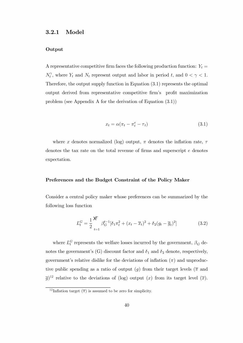
3.2.1 Model

Output

A representative competitive Þrm faces the following production function: Yt =

Nγt , where Yt and Nt represent output and labor in period t, and 0 < γ < 1.

Therefore, the output supply function in Equation (3.1) represents the optimal

output derived from representative competitive Þrms proÞt maximization

problem (see Appendix A for the derivation of Equation (3.1))

xt = α(πt − πet − τ t) (3.1)

where x denotes normalized (log) output, π denotes the inßation rate, τ

denotes the tax rate on the total revenue of Þrms and superscript e denotes

expectation.

Preferences and the Budget Constraint of the Policy Maker

Consider a central policy maker whose preferences can be summarized by the

following loss function

LGt =1

2

TXt=1

βt−1G [δ1π2t + (xt − xt)2 + δ2(gt − gt)2] (3.2)

where LGt represents the welfare losses incurred by the government, βG de-

notes the governments (G) discount factor and δ1 and δ2 denote, respectively,

governments relative dislike for the deviations of inßation (π) and unproduc-

tive public spending as a ratio of output (g) from their target levels (π and

g)12 relative to the deviations of (log) output (x) from its target level (x).

12Inßation target (π) is assumed to be zero for simplicity.

40

Equation (3.2) reveals that policy maker dislikes the deviations of inßation,

output and public spending from their target levels. A non-zero output target

x could possibly represent the Þrst best-level of (or bliss point for) output;

that is, the level of output without both tax and non-tax distortions (e.g. due

to labor market imperfections). Similarly, a non-zero public spending target g

could represent the optimal share of output on public spending. Nevertheless,

the target levels of output and public spending (x and g) as well as weights

attached to these targets (δ1 and δ2) reßect the political and the institutional

structure of the economy (see Chapter 4 for more detail).

The budget constraint of the government is given as follows

gt = τ t + πt (3.3)

This budget constraint indicates that distortionary taxes and seigniorage

are the two sources of Þnancing for the government outlays.13 The budget con-

straint creates the link between the monetary and Þscal policies. (see Appendix

B for the derivation of Equation (3.3))

3.2.2 Features of the Equilibrium

In this model, the central policy maker (government) controls both Þscal and

monetary policies. Also the policy maker is assumed to control directly the

inßation rate (π) by controlling nominal money supply.14 Additionally, the

policy maker sets the tax rate (τ) and government spending (g). Furthermore,

monetary and Þscal policy decisions are made simultaneously.

13Borrowing is excluded as a source of Þnance. The issues of public borrowing will beconsidered in Chapter 5.14This follows from the assumption that money demand equation is based on simple

quantity theory framework (See Appendix B). Therefore, the rate of inßation simply equalsto the rate of growth of the nominal money supply.

41

Formally speaking, government optimally selects its policies by minimiz-

ing the loss function subject to the budget constraint and the output supply

function and with respect to π, τ and g. Equilibrium values of inßation, the

tax rate, public spending and output are as follows (see Appendix C for the

derivations of (3.4)-(3.7))

πt =2δ2δ1Ψ[1

αxt + gt] (3.4)

τ t =δ2α2Ψgt −z

1

αxt (3.5)

gt = Ψ[φgt −1

αxt] (3.6)

xt = zxt − δ2αΨgt (3.7)

where φ = δ2α2+ 2δ2

δ1,Ψ = 1

(1+φ),z = (1− δ2

α2Ψ) > 0.

As it is evident from Equation (3.4) there are two sources of the non-

zero equilibrium inßation rate. In other words, inßation bias exists due to the

presence of non-zero output and public spending targets; x and g, respectively.

Therefore, a rise in x and/or g raises equilibrium inßation. Similarly, as it is

clear from Equation (3.5) the equilibrium tax rate is determined by x and

g. An increase in g raises both inßation and taxes since they represent the

two alternative methods of Þnancing a higher level of public spending. On

the other hand, while a rise in x raises equilibrium inßation rate, it lowers tax

rates, as expected. Moreover, it is evident from Equation (3.6) and (3.7), while

a rise in g raises equilibrium public spending it lowers output. Similarly, while

a rise in x raises equilibrium output it lowers public spending.

42

Finally, in this section, the deviations of equilibrium values of output and

public spending from their respective target levels (output gap and public

spending gap, respectively) and the inßation rate that the government is con-

cerned about will be presented in Table 3.1.

Table 3.1 Output Gap, Public Spending Gap and Inßation Rate:

The Benchmark Model

(xt − xt) = δ2αΨ[ 1

αxt + gt]

(gt − gt) = Ψ[ 1αxt + gt]πt =

2δ2δ1Ψ[ 1

αxt + gt]

Table 3.1 indicates that the equilibrium values of output and public spend-

ing are lower than their respective target values. Similarly, equilibrium inßa-

tion rate is above its respective target level.

There is a trade-off between achieving higher output and public spending.

This is clear from Equation (3.6) and (3.7), the higher the public spending

(output) target, the lower is the equilibrium output (public spending) and

therefore the larger is its deviation from target. This trade-off arises due

to the Þnancing requirement. Higher government expenditure is Þnanced by

raising taxes and/or inßation. It follows from Equation (3.5), that the higher

the g, the higher will be the taxes. This will, in turn, lower output by reducing

proÞtability. As a result, the higher the public expenditure target (g) the larger

the output and public spending gaps and inßation rate.

43

3.3 The Basic Dynamic Model: Extending the

BenchmarkModel with Productive Public

Spending

Recall that public spending is assumed to be totally unproductive in the bench-

mark model analyzed above and hence has no favorable effect on productivity

and output either in the current or in the following period. However, in prac-

tice, governments make separate decisions regarding how much to spend on

different categories of public spending. Furthermore, as discussed before, the

decision to spend on productive categories instead of on unproductive but pop-

ular categories can have crucially different consequences on productivity and

output. Therefore, this section extends the above (static) benchmark model

into a simple dynamic, i.e. two-period (T = 2), model by considering the

productivity enhancing role of public spending. Hence, the main feature of

the basic dynamic model is a distinction between the productive (gp) and non-

productive public spending (gnp). Therefore, the benchmark model is modiÞed

as follows.

3.3.1 Model

Output

In this model, the representative competitive Þrm faces the following form of

the above given production function (see Section 3.2.1): Yt = AtNγt , (0 <

γ < 1), where At represents the level of productivity in period t and is as-

sumed to be enhanced by the previous periods productive public spending.

Appendix D derives the following normalized output supply function from the

representative competitive Þrms proÞt maximization problem as above,

44

xt = α(πt + ρgpt−1 − πet − τ t) (3.8)

where ρ may be thought as productivity coefficient measuring extent by

which one periods productive public spending improves the productivity (and

hence output) in the following period.15 ,16 All other variables are as deÞned

before.


With the analytical distinction between productive (gp) and unproductive pub-

lic spending (gnp), the policy makers preferences can be represented by the

following loss function

LGt =1

2

T=2Xt=1

βt−1G [δ1π2t + (xt − xt)2 + δ2(gnpt − gnpt )2 + δ3(gpt − gpt )2] (3.9)

where gpt and gnpt are used as the policy makers target for productive

and non-productive public spending, respectively.17 All other variables are as

deÞned before.

15This is in line with most of the literature (e.g. Rogoff, 1990; Dur et al., 1998; andPersson and Tabellini, 2000). See Section 2.3.2.16Note that ρ = ζ

γ , where ζ is the coefficient of productivity measuring extent by whichone periods productive public spending improves the (log) productivity in the followingperiod and γ is a parameter of production function (see Appendix D for more detail).17Nevertheless, as the beneÞcial effects of productive public spending are not usually

realized until future periods this spending can be visible in the future and may not yieldinstant (contemporaneous) utility to the policy maker, and hence may not form part ofhis current utility function. On the contrary, non-productive spending can be immediatelyobserved by voters and hence increases the popularity of the incumbent government (or thepolicy maker). Thus, non-productive spending may yield instant utility to the policy maker.These arguments suggest that the loss function may take the following form,

45

Similarly, the budget constraint of the government can be simply modiÞed

as follows

gnpt + gpt = πt + τ t (3.10)

This modiÞed budget constraint suggests that distortionary taxes and seignior-

age are two sources of Þnancing for the government outlays. Note that a bal-

anced budget rule is assumed in each and every period; that is, borrowing

is excluded as a source of Þnance to abstract from issues of debt dynamics

(Chapter 5 will relax this assumption). Thus, the only intertemporal link in

this set-up is due to the favorable effect of productive spending on output in

the next period.

3.3.2 Equilibrium Macroeconomic Outcomes

Characterization of Equilibrium

In this two-period set-up, equilibrium outcomes are derived by backwards in-

duction. More speciÞcally, policy outcomes in the Þnal-period (t = 2) are

derived Þrst, for a given level of gp1, and then, equilibrium outcomes in the

Þrst-period (t = 1) are derived.

In the Þnal-period, gp is not among the choice variables in this two-period

set-up since the principal beneÞt of gp is realized with one-period lag. Ac-

cordingly, the vital decision concerning the composition of the public spending

LGt =1

2

T=2Xt=1

βt−1G [δ1π2t + (xt − xt)2 + δ2(gnpt − gnpt )2]

Nevertheless, this loss function is a special case (δ3 = 0) of Equation (3.9) and qualitativenature of the results of this chapter would not change if we employ the above equation insteadof Equation (3.9) (see Ismihan and Ozkan, 2002).

46

is made in the Þrst-period, which will be analyzed below. Therefore, in the

Þnal-period, the central policy maker chooses π2, τ 2 and gnp2 subject to the

constraints, for a given level of gp1. Table 3.2 contains the Þnal-period opti-

mal policy outcomes, for a given level of gp1 (see Appendix E for the technical

details on the derivation of the result for t = 2 ).

Table 3.2 Final-period Optimal Policy Outcomes:

The Basic Dynamic Model

π2 =2δ2δ1Ψ[ 1

αx2 + g

np2 − ρgp1]

x2 = zx2 − δ2αΨgnp2 +

δ2αΨρgp1

gnp2 = Ψ[φgnp2 + ρgp1 − 1

αx2]

τ2 = ρzgp1 + δ2α2Ψgnp2 −z 1

αx2

Note: φ = δ2α2+ 2δ2

δ1,Ψ = 1

(1+φ),z = (1− δ2

α2Ψ) > 0.

Table 3.3 Equilibrium Macroeconomic Outcomes in t = 1 and t = 2:

The Basic Dynamic Model

gp1 = Θ[δ3δ2Ψgp1 − gnp1 + Γgnp2 − 1

αx1 +

Γαx2]

gnp1 = − δ3δ2Θgp1 + (1−Φ) gnp1 − ΛΘgnp2 − 1

αΦx1 − ΛΘ 1

αx2

π1 =2δ2δ1[ δ3δ2Θgp1 + Φg

np1 + ΛΘg

np2 + Φ

1αx1 + ΛΘ

1αx2]

x1 = − δ2α[ δ3δ2Θgp1 + Φg

np1 + ΛΘg

np2 + ΛΘ

1αx2] +Υx1

τ 1 =δ2α2[ δ3δ2Θgp1 + Φg

np1 + ΛΘg

np2 + ΛΘ

1αx2]−Υ 1

αx1

gnp2 = Ψ(φ+ ρΓΘ)gnp2 − 1αΨΞx2 + ρΨ[

δ3δ2ΨΘgp1 −Θgnp1 −Θ 1

αx1]

π2 =2δ2δ1ΨΞ[ 1

αx2 + g

np2 ]− ρ2δ2δ1 Ψ[ δ3δ2ΨΘg

p1 −Θgnp1 −Θ 1

αx1]

x2 = (z+ δ2α2ΨρΓΘ)x2 − δ2

αΨΞgnp2 +

δ2αΨρ[ δ3

δ2ΨΘgp1 −Θgnp1 −Θ 1

αx1]

τ 2 = (δ2α2Ψ+ ρΓΘz)gnp2 −zΞ 1

αx2 + ρz[ δ3δ2ΨΘg

p1 −Θgnp1 −Θ 1

αx1]


δ1,Ψ = 1

(1+φ),z = (1− δ2

α2Ψ) > 0, D = 2δ2

δ1Ψ2 +Ψ,Λ =

ρβGD,Γ =ΛΨ= ρβG

ΨD,Ω =

(δ3δ2+ρΛ)

Ψ,Θ = 1

(1+Ω), 0 < Φ = ΨΩ

(1+Ω)< 1,Ξ =

1− ρΘΓ > 0,Υ = ¡1− δ2

α2Φ

¢> 0.

47

As mentioned before, the decision regarding the composition of public

spending is made by policy maker in the Þrst period. Therefore, the policy

maker makes his choice by distributing distortions among both intratemporal

and intertemporal instruments in t = 1. Formally speaking, the central policy

maker chooses π1, τ1, gnp1 and gp1 subject to the constraints in the Þrst period.

Table 3.3 contains the equilibrium outcomes in t = 1 as well as in t = 2 (see

Appendix E for the technical details on the derivation of the result for t = 1).

Favorable Effects of Productive Public Spending on Future Macroe-

conomic Performance

It could be useful to compare the above results with the results in the

static benchmark case. To this end, Table 3.4 is formed below, which shows

the output gap, public spending gap and inßation rate in the second period,

in line with Table 3.1 of the benchmark case.

Table 3.4 Output Gap, Public Spending Gap and Inßation Rate

in t = 2: The Basic Dynamic Model

(x2 − x2) = δ2αΨ[ 1

αx2 + g

np2 − ρgp1]

(gnp2 − gnp2 ) = Ψ[ 1αx2 + gnp2 − ρgp1]π2 =

2δ2δ1Ψ[ 1

αx2 + g

np2 − ρgp1 ]

As it is clear from Table 3.4, the beneÞcial effect of the previous periods

productive public spending on the current periods output clearly mitigates the

trade-off between public spending and output; thus, lowers the distortions in

the economy. Nevertheless, even though the intratemporal trade-offmentioned

in the static benchmark case still remains, higher productive public spending in

the previous period now raises the next periods equilibrium output (and hence

48

the tax base).18 Likewise, while higher g2 and x2 enhances both the output

and unproductive public spending gaps, higher gp1 helps to reduce them via

the intertemporal link.

The interesting result is that the beneÞcial effects of productive public

spending are not limited to output and inßation but also include future non-

productive spending.19 In other words, policy maker could expand his future

resources by spending today on productive activities such as core infrastruc-

ture, R&D, and education, and, in turn, this would allow the policy maker to

increase future non-productive or popular public spending.

Proposition 1 formalizes the above arguments.

Proposition 1 The higher the productive public spending in the Þrst period

the lower the inßation (and inßation bias), non-productive public spending gap

and output gap; hence, the better the macroeconomic performance in the Þnal

period. That is, the higher the gp1, the lower the π2, (gnp2 − gnp2 ) and (x2 − x2).

Proof. The derivative of π2 with respect to gp1 is

−2δ2δ1ρΨ,which is unambigu-

ously negative for all values of ρ and Ψ. Similarly, the derivative of (gnp2 − gnp2 )with respect to gp1 is −ρΨ, which is again negative. The derivative of (x2−x2)with respect to gp1 is −ρΨ δ2

α, which is also unambiguously negative.

As is clear from Proposition 1, the higher the size of the productivity

coefficient ρ the higher the size of the beneÞcial effect of productive spending

18Also note that higher productive public spending committed in the previous periodraises the next periods equilibrium tax rate by enhancing the tax base (see Table 3.3). Thisis the indirect beneÞcial effects of higher productive public spending. This result is in linewith the result obtained from Persson and Tabellinis (2000) model on public investmentand economic growth, which is discussed in Section 2.3.19It should be noted that the results of this chapter are derived under the absence of

electoral uncertainty; therefore, these results and associated conclusions are conditional onthis implicit assumption that the incumbent government will hold the office in the secondperiod (i.e. there is electoral certainty). This assumption will be relaxed in the followingchapters.

49

on the next periods macroeconomic performance. The determinants of ρ will

be discussed in the next chapter.

Productive vs. Non-Productive Spending: Trade-offs and Asymme-

tries

Table 3.5 provides the comparative statics, which will be utilized in analyz-

ing the trade-offs and associated asymmetries arising from the productivity

enhancing role of productive public spending and the existence of budget con-

straint.

Table 3.5 Comparative Statics: The Basic Dynamic Model

↑ gp1 ↑ gnp1 ↑ gnp2 ↑ x1 ↑ x2gp1 + − + − +

gnp1 − + − − −π1 + + + + +

x1 − − − + −τ 1 + + + − +

gnp2 + − + − −π2 − + + + +

x2 + − − − +

τ 2 + − + − −

Note: + indicates positive effect and − indicates negative effect.

As mentioned before, by spending on productive activities in the current

period, the policy maker increases his future resources via the intertemporal

link between gp1 and x2; hence, the policy maker could increase non-productive

spending in the next period. However, as can be seen from Table 3.5, there

is an intratemporal trade-off between productive and non-productive spending

50

in the Þrst-period; that is, the higher the productive spending target the lower

the non-productive public spending and vice versa. This trade-off emerges

due to the existence of budget constraint20 and the trade-off between public

spending (productive as well as non-productive spending) and output in the

Þrst-period, as mentioned in benchmark case. Thus the existence of the above

mentioned intertemporal link and the intratemporal trade-offs results in in-

teresting asymmetries. For example, there is an asymmetry with respect to

the effects of productive vs. non-productive spending targets on future output,

public spending and inßation, as is seen from Table 3.5. Furthermore, there is

another asymmetry between the effects of current and future non-productive

public spending targets on current actual productive and non-productive pub-

lic spending. As can be seen from Table 3.5, a rise in gnp1 decreases (raises)

productive (non-productive) public spending in t = 1 while a rise in gnp2 raises

(lowers) it. This asymmetry is due to the above mentioned trade-off between

gnp1 and gp1 and the intertemporal link between g

p1 and x2. That is, on the one

hand, a rise in productive spending is only possible by lowering non-productive

spending in t = 1 and vice versa; on the other hand, a rise in non-productive

spending in t = 2 is only possible by raising productive spending in t = 1. Sim-

ilarly, while there exists an additional asymmetry between the effects of future

output target on productive and non-productive public spending in t = 1,

there is not an asymmetry between the effects of current output target on

productive and non-productive public spending in t = 1.

The key results are summarized as follows:

The higher the productive (non-productive) public spending target thehigher the actual productive (non-productive) public spending and hence

20The budget constraint of the government [Equation (3.11)] can be re-written as follows

gnpt = πt + τ t − gptAs is clear from this equation, a rise in productive spending lowers non-productive spend-

ing and vice versa.

51

the lower (higher) the share of non-productive spending in total public

spending in the Þrst period. As a result, the lower (higher) the inßation

and the higher (lower) the non-productive public spending and output;

hence, the better (worse) the macroeconomic performance in the Þnal pe-

riod. That is, the higher the gp1 ( gnp1 ) the lower (higher) the π2 and the

higher (lower) gnp2 and x2.

The higher are non-productive spending target and output target in fu-ture, the lower (higher) must be the productive (non-productive) public

spending and hence the lower must be the share of non-productive spend-

ing in total public spending today. That is, the higher are gnp2 and x2 the

lower is the gnp1 ( gp1).

Therefore, there exist both intratemporal and intertemporal trade-offs of

policy making and associated asymmetries affecting the composition of public

spending in the basic dynamic macroeconomic policy making framework. Next

chapter will discuss the political economy of the composition of public spending

and this will shed some light on the above results.

Finally, given the above results on the macroeconomic effects of productive

vs. non-productive public spending, it is interesting to analyze the macroe-

conomic consequences of the policy makers public spending decisions for the

whole period (i.e. Þrst and Þnal periods taken together).

For instance, even though there is not any asymmetry with respect to the

effects of productive vs. non-productive spending targets on current inßation,

the size of the effect of productive public spending target is lower vis-a-vis

non-productive spending targets in t = 1 (i.e. ∂π1/∂gnp1 > ∂π1/∂g

p1 > 0).

Therefore, recalling that there is an asymmetry with respect to the effects

of productive vs. non-productive spending targets on future inßation (i.e.

∂π2/∂gnp1 > 0 and ∂π2/∂g

p1 < 0), productive public spending produces lower

52

inßation, compared to non-productive public spending, when the whole period

is considered.

Another interesting as well as related result is that transferring resources

from non-productive public spending to productive spending (via raising pro-

ductive spending target) lowers current non-productive spending but it may

raise future non-productive spending by larger amount than the lost non-

productive public spending in the current period, depending on the size of

the productivity coefficient ρ. More formally, if ρ is larger than one then the

lost non-productive public spending in the Þrst period (|∂gnp1 /∂gp1|) is lowerthan the increment in non-productive spending in the Þnal period (∂gnp2 /∂g

p1)

and vice versa, if ρ is lower than one. Similarly, if ρ is larger than one then

the reduction in output in the current period (|∂x1/∂gp1|) is lower than theincrement in output in the Þnal period (∂x2/∂g

p1) and vice versa, if ρ is lower

than one.

3.4 Decentralized Policy Making

In this section, the previous analysis is extended by considering decentralized

monetary and Þscal policy making. In other words, we consider a policy mak-

ing framework such that government acting through the Þscal authority per-

forms the Þscal policy and an independent central bank (monetary authority)

performs the monetary policy.

3.4.1 The Decentralized Benchmark Model

This section extends the static centralized policy making framework of Sec-

tion 3.2 into a decentralized policy making framework.21 In this new set-up,

21See, for example, Alesina and Tabellini (1987), Jensen (1994), Debelle and Fischer(1994), Beetsma and Bovenberg (1997a, 1997b, 1999) and Ozkan (1998, 2000) for similarvariants of the decentralized benchmark model.

53

government decides about taxes and spending while the central bank chooses

the inßation rate. Thus, the only but crucial difference in this set-up is that

each authority has its own preferences and policy decisions are taken simulta-

neously and non-cooperatively. Therefore, while preferences of the government

(G) is the same as Equation (3.2), monetary authoritys (M) preferences can

be summarized by the following loss function,

LMt =1

2

TXt=1

βt−1M [µ1π2t + (xt − xt)2 + µ2(gt − gt)2] (3.11)

where LMt denotes the welfare losses incurred by the independent central

bank, µ1 and µ2 denote, respectively, the central banks relative dislike for

the deviations of inßation (π) and public spending (g) from their target levels

(π and g),22 and µ1 is assumed to be greater than δ1. Similarly, βM is the

central banks discount factor and it is assumed to be greater than βG. That

is, the independent central bank is more conservative than elected government

(µ1 > δ1) and does not discount the future at a lower rate than the elected

government (βM > βG).

Output supply function and the budget constraint of the government are

the same as in the benchmark case of Section 3.2. That is, they are represented

by Equation (3.1) and (3.3), respectively.

As the policy decisions are taken simultaneously and non-cooperatively

in this one-period model, government and independent central bank plays a

one-shot Nash game. In other words, while the government decides about

taxes and spending, taking central banks action and expectations as given,

the central bank chooses the inßation rate, taking the governments action and

expectations as given.

22Again, inßation target (π) is assumed to be zero for simplicity.

54

Nash equilibrium values of inßation rate, tax rate, public spending and out-

put are contained in Table 3.6, where superscript d denotes the decentralized

case (see Appendix F for the derivation of equilibrium values)

Table 3.6 Equilibrium Macroeconomic Outcomes:

Decentralized Benchmark Case

πdt =δ2µ1Ψ0[ 1

αxt + gt]

xdt = z0xt − δ2αΨ0gt

gdt = Ψ0[φ0gt − 1

αxt]

τ dt =δ2α2Ψ0gt −z0 1

αxt

Note: φ0 = δ2α2+ δ2

µ1,Ψ0 = 1

(1+φ0) ,z0 = 1− δ2

α2Ψ0 > 0.

It is clear that these results are similar to the those of the centralized case

(Section 3.2). Hence they could be interpreted in the same way. However,

the crucial difference between the decentralized and centralized policy making

is that the equilibrium values of output and inßation are lower under decen-

tralized policy making. Lower value of equilibrium inßation is due to the fact

that the independent central bank is more conservative than the elected gov-

ernment (µ1 > δ1).23,24 This result is in line with the well-known argument

in the literature of central bank independence that the delegation of monetary

policy making powers to independent central banks leads to a lower inßation

(see, for example, Rogoff, 1985).

Similarly, the lower level of equilibrium output under decentralized policy

making is due to the detrimental effects of higher taxes on output. That is,

lower level of inßation involves higher resources elsewhere to Þnance public

23Provided that µ1 > δ1, thenδ2

µ1Ψ0 < 2δ2

δ1Ψ and thus equilibrium level of inßation is lower

under decentralized policy making compared to the centralized policy making.24Also note that central bank does not internalize the budget constraint of the government.

55

spending, which results in higher equilibrium taxes and hence a lower equilib-

rium level of output, given the detrimental effects of taxes on output in this

model.

3.4.2 The Decentralized Dynamic Model

In this section, the basic dynamic model of Section 3.3 is extended to a decen-

tralized policy making framework. In this new two-period framework, govern-

ment and independent central bank play a Nash game in both periods. The

only change in this new set-up is as set-out above. That is, while preferences

of the government is the same as Equation (3.9), central banks preferences

can be summarized by the Equation (3.11). Similarly, output supply function

and the budget constraint of the government are represented by Equation (3.8)

and (3.10), respectively.

As in Section 3.3, equilibrium outcomes are derived by backwards induc-

tion. Table 3.7 contains the equilibrium outcomes in t = 1 as well as in t = 2

for the dynamic decentralized model.25

As it is clear from Table 3.7, main Þndings of Section 3.3 also hold for the

decentralized case. For example, the higher the productive (non-productive)

public spending in the Þrst period the lower (higher) the inßation (and inßation

bias) and the higher (lower) non-productive public spending and output in the

Þnal period. Similarly, the higher the non-productive spending and output

targets in future, the lower (higher) must be the productive (unproductive)

public spending today.

25Equilibrium results are derived by backwards induction as in Appendix E. That is, fora given gp1 , policy outcomes and Þscal authoritys welfare losses for t = 2 are derived Þrst.Then, equilibrium outcomes for t = 1 are derived.Also note that government and independent central bank play a Nash game as in Appendix

F in both periods (i.e. in t = 1 and t = 2). For example, central bank chooses π2 to minimizeEquation (3.11) while the government chooses τ2 and g

np2 to minimize Equation (3.9) subject

to the constraints, simultaneously and non-cooperatively (i.e. by taking each others actionand expectations as given).

56

Table 3.7 Equilibrium Macroeconomic Outcomes

in t = 1 and t = 2: (Dynamic) Decentralized Case

gp,d1 = Θ0[ δ3δ2Ψ0

gp1 − gnp1 + Γ0gnp2 − 1αx1 +

1αΓ0x2]

gnp,d1 = −δ3δ2Θ0gp1 + (1−Φ0) gnp1 − Λ0Θ0gnp2 − 1

αΦ0x1 − Λ0Θ0 1αx2

πd1 =δ2µ1[ δ3δ2Θ0gp1 + Φ

0gnp1 + Λ0Θ0gnp2 + Φ

0 1αx1 + Λ

0Θ0 1αx2]

xd1 = − δ2α[ δ3δ2Θ0gp1 + Φ

0gnp1 + Λ0Θ0gnp2 + Λ

0Θ0 1αx2] +Υ

0x1

τd1= δ2

α2[ δ3δ2Θ0gp1 + Φ

0gnp1 + Λ0Θ0gnp2 + Λ

0Θ0 1αx2]−Υ0 1αx1

gnp,d2 = Ψ0[φ0gnp2 + ρgp,d1 − 1

αx2]

= Ψ0(φ0 + ρΓ0Θ0)gnp2 − 1αΨ0Ξ0x2 + ρΨ0[ δ3δ2Ψ0Θ

0gp1 −Θ0gnp1 −Θ0 1αx1]πd2 =

δ2µ1Ψ0[ 1

αx2 + g

np2 − ρgp,d1 ]

= δ2µ1Ψ0Ξ0[ 1

αx2 + g

np2 ]− ρ δ2µ1Ψ

0[ δ3δ2Ψ0

Θ0gp1 −Θ0gnp1 −Θ0 1αx1]xd2 = z0x2 − δ2

αΨ0gnp2 +

δ2αΨ0ρgp,d1

= (z0 + δ2α2Ψ0ρΓ0Θ0)x2 − δ2

αΨ0Ξ0gnp2 +

δ2αΨ0ρ[ δ3

δ2Ψ0Θ0gp1 −Θ0gnp1 −Θ0 1αx1]

τd2 = ρz0gp,d1 + δ2α2Ψ0gnp2 −z0 1

αx2

= ( δ2α2Ψ0 + ρΓ0Θ0z0)gnp2 −z0Ξ0 1

αx2 + ρz0[ δ3

δ2Ψ0Θ0gp1 −Θ0gnp1 −Θ0 1αx1]

Note: φ0 = δ2α2+ δ2µ1,Ψ0 = 1/(1+φ0),z0 = 1− δ2

α2Ψ0, D0 = α2δ1δ2+δ2µ21+α

2µ21α2µ21

Ψ02,

Λ0 = ρβGD0,Γ0 = Λ0

Ψ0 =ρβGΨ0 D

0,Ω0 =(δ3δ2+ρΛ0)Ψ0 ,Θ0 = 1

(1+Ω0) , 0 < Φ0 = Ψ0Ω0

(1+Ω0) <

1,Ξ0 = 1− ρΘ0Γ0 > 0,Υ0 = ¡1− δ2

α2Φ0

¢> 0.

It is clear that in the static decentralized benchmark case, where all public

spending is unproductive, central bank independence is an institutional solu-

tion for lowering the inßation bias. However, this may not be the case in the dy-

namic decentralized model given the beneÞcial effects of current productivity-

enhancing public spending on the next periods macroeconomic performance26

26The size of the beneÞcial effect of productive public spending is expected to be high fordeveloping countries since the productivity of public investment (ρ) is expected to be highfor them (see, for example, World Bank, 1994 and Azariadis and Lahiri, 2002).

57

as well as on the distortions in the economy (e.g. inßation bias).27 That is,

central bank independence by leading to lower inßation diminishes the avail-

able resources for public spending (by lowering seigniorage revenue) and hence

results in a fall in productive spending in the Þrst period28 and, as a result,

it may have unfavorable effects on future inßation. Therefore, central bank

independence may not result in lower level of equilibrium inßation when the

whole period is considered, i.e. Þrst and Þnal periods taken together.

To achieve a more credible monetary policy and to reduce the political

manipulation of inßation and the inßation bias, many developing countries,

including Turkey, as well as developed countries granted high degree of inde-

pendence to their central banks during the last Þfteen years.29 Nevertheless,

recent experiences of developing countries have shown that the credibility of

monetary policy does not only depend on the independence of the monetary

authority but also crucially depends on the overall stance of macroeconomic

policy (see, for example, Agenor and Montiel, 1996). For example, credibility

cannot be achieved if Þscal policy is not sustainable and/or consistent with

the monetary policy, even in the case of fully-independent central bank. The

results of this section also suggest that it is important to take into account the

other dynamics of Þscal policy, such as the beneÞcial effects of productivity-

enhancing public spending on future macroeconomic performance, in designing

optimal macroeconomic policy making framework.

27Also recall from the previous analysis that productive public spending produces lowerinßation, compared to non-productive public spending, when the whole period is considered.28Moreover, as discussed previously, lower level of inßation also involves higher resources

elsewhere to Þnance public spending, which results in higher equilibrium taxes and hence alower equilibrium level of output due to the detrimental effects of taxes on output.29See Kirshner (2001), Romer (2001) and Agenor and Montiel (1996) for the literature on

central bank independence and on other related topics such as inßation targeting.

58

3.5 Conclusion

This chapter has attempted to study how the governments public spending

decisions affect overall macroeconomic performance. To this end, a macroe-

conomic policy making framework is developed by linking the overall macroe-

conomic performance of an economy to the public spending decisions. This

framework, in turn, has enabled us to analyze the consequences of the two

types of public spending (productive vs. non-productive public spending) on


The main result of this chapter is that a change in the composition of pub-

lic spending can play a crucial role in future macroeconomic performance. For

instance, it has been shown that if public resources are channelled into pro-

ductive public spending, such as spending on the core infrastructure, R&D,

and education, the macroeconomic performance will be improved in the fu-

ture; and vice versa, if public resources are channelled to non-productive but

popularity enhancing public spending, such as spending on public wage in-

creases and social transfers. This is due to the beneÞcial effect of productive

public spending on the next periods output and hence on the distortions in

the economy. The interesting result is that the beneÞcial effects of productive

spending are not only limited to future output and inßation but also includes

future non-productive spending. In other words, policy maker could expand his

future resources by spending today on productive activities and, in turn, this

would allow the policy maker to increase even future non-productive or popular

spending. Additionally, another related and interesting result is that transfer-

ring resources from non-productive public spending to productive spending

lowers current non-productive spending but it can raise future non-productive

spending by larger amount than the lost non-productive public spending in

the current period, if the size of the productivity coefficient ρ is larger than

one. Likewise, if ρ is larger than one then the reduction in output in the cur-

59

rent period is lower than the increment in output in the next period and vice

versa, if ρ is lower than one. Finally, it has been also shown that productive

public spending produces lower inßation, compared to non-productive public

spending, when the whole period is considered.

The main Þndings of this chapter also hold under both centralized and de-

centralized policy making frameworks. However, given the favorable effects of

productive public spending on future macroeconomic performance, the delega-

tion of monetary policy making to an independent central bank may not result

in lower inßation in the long-term. In many developing countries seigniorage

is an important source of Þnance (see Agenor and Montiel, 1996) and the

productivity of public investment is expected to be high (World Bank, 1994);

therefore, in such countries central bank independence may harm inßation

performance in the long-term. Therefore, it is important to take into account

the dynamics of public spending and hence Þscal policy choices, in designing

optimal macroeconomic policy making framework.

The main Þndings in this chapter reveal that policy makers face both in-

tratemporal and intertemporal trade-offs while making the choice for the com-

position of overall public spending. Therefore, political economy factors, such

as political instability and electoral uncertainty, can play a crucial role on the

policy makers choice. The political economy and related issues will be dis-

cussed in the next chapter and this will shed some light on the above results.

Moreover, the issues of debt dynamics will be discussed in Chapter 5.

60

CHAPTER 4

THE POLITICAL ECONOMY OF THECOMPOSITION OF PUBLIC SPENDING

AND FISCAL ADJUSTMENT

4.1 Introduction

The previous chapter has developed a macroeconomic policy making frame-

work that enabled us to investigate the macroeconomic consequences of the

policy makers choice for the composition of overall public spending. This

chapter attempts to analyze the effects of several politico-economic factors on

the composition of public spending and macroeconomic outcomes. In other

words, the current chapter aims to extend the previous chapters analysis by

exploring the role of a set of political economy factors, such as political instabil-

ity and electoral uncertainty, on the policy makers choice for the composition

of overall public spending.

This chapter particularly focuses on the role of socio-political instability

on public spending decisions and overall macroeconomic performance.1 In line

1See Section 2.3 for an overview of the literature on the role of socio-political factors onpublic spending policies and macroeconomic performance.

61

with this aim, the policy makers choice for one type of public spending over the

other is taken to be determined by a number of socio-political factors such as

the degree of income inequality, social and ethnic fractionalization, which may

affect the level of political instability and hence the public spending decisions

of the incumbent governments. Additionally, a high level of political instabil-

ity may lead to myopic policies (via electoral uncertainty),2 in the form of low

levels of productive spending. This possibility arises due to the intertemporal

nature3 of productive public spending that creates an opportunity for a strate-

gic political behavior. Thus, this chapter attempts to provide some political

economy explanations to the myopic and populist spending policies and asso-

ciated undesirable macroeconomic performances of some developing countries

with unstable and polarized socio-political environment.4

The second issue that is considered in this chapter is the role of qualitative

aspects of Þscal policy making on macroeconomic performance. More speciÞ-

cally, this chapter attempts to develop a framework to provide insights into the

understanding of recent empirical results on the detrimental effects of corrup-

tion and favoritism on the level of productivity of productive public spending,

such as public investment in infrastructure, and hence on output performance

(see, for example, Mauro, 1997; and Tanzi and Davoodi, 1998).5

The third and last issue that is considered in this chapter is related to

expansionary Þscal adjustments. The current line of research emphasizes the

expansionary consequences of some types of Þscal adjustments (see, for exam-

ple, Giavazzi and Pagano, 1990; Perotti, 1996; Alesina and Ardagna, 1998;

and Alesina et al., 1998).6 There is growing empirical evidence that Þscal con-

2Recall that Chapter 3 implicitly assumes electoral certainty. This chapter will relax thatassumption.

3Productive public spending committed in the current period can enhance future pro-ductivity and output. Thus, productive public spending connects current government touncertain future government.

4Chapter 5 will analyze the role of political instability and electoral uncertainty on thepublic borrowing policies and macroeconomic performance.

5See Chapter 2 for more detail.6See Chapter 2 for more detail.

62

solidations involving largely public investment cuts are shown to be contrac-

tionary, while Þscal adjustments that entail largely current or social transfer

expenditure cuts are expansionary. Therefore, this chapter also attempts to

provide a political economy explanation for the role of the composition of Þscal

adjustments on macroeconomic performance.

The remainder of this chapter is organized as follows. Section 4.2 ana-

lyzes the political economy determinants of the policy makers choice on the

composition of public spending and hence on the macroeconomic performance,

by utilizing the macroeconomic framework developed in the previous chapter.

More speciÞcally, the effects of the socio-political instability and corruption on

macroeconomic performance will be investigated in Section 4.2, by focusing

on the role of productivity-enhancing public spending. Section 4.3 explores

the role of the composition of Þscal adjustments on their consequences for

macroeconomic performance and provides a political economy explanation to

it. Finally, Section 4.4 concludes the chapter.

4.2 Political Economy of the Composition of

Public Spending

To analyze the role of a number of political economy factors on the policy

makers public spending decisions and on macroeconomic performance, this

section utilizes the basic dynamic model. In this model, the political structure

and factors, such as political instability and electoral uncertainty, may affect

the governments7 public spending decisions and macroeconomic outcomes in

various ways, by affecting: (1) the governments spending targets (gp and

gnp) as well as the weights attached to these targets (δ2 and δ3); (2) the

7This chapter continues to utilize a centralized policy making framework but the mainresults also hold under a decentralized policy making framework.

63

governments discount factor (βG) and (3) the coefficient of productivity (ρ).

The following sub-sections formally analyze these channels.

4.2.1 Political Instability and Polarization

Political instability and polarization can manifest itself directly or indirectly

in the public spending decisions.8 Political instability, for instance, may be

directly reßected in the public spending decisions (via policy makers targets)

due to the characteristics of the socio-political structure. It may also manifest

itself through elections. Therefore, Þrst the effects of the characteristics of the

socio-political structure on public spending decisions and hence on macroeco-

nomic performance will be analyzed and then the role of electoral uncertainty

on public spending decisions will be investigated in the following two sub-

sections, respectively.

Income Inequality, Social Fractionalization, Weak Governments and

Populism

As mentioned in Chapter 2, a number of characteristics of the political environ-

ment, such as the existence of weak or strong governments, income and wealth

inequality and social fractionalization, may have signiÞcant effects on political

instability and public spending decisions. Politically weak governments, for in-

stance, tend to cut public investment rather than current spending compared

to politically strong governments (Roubini and Sachs, 1989a). Furthermore,

a high degree of income and wealth inequality, especially in developing coun-

tries, usually give rise to an unstable political environment (Alesina and Per-

otti, 1996). Governments in such atmosphere have greater incentives to follow


64

populist policies which favor redistributive public spending.9 Moreover, higher

level of social or ethnic fractionalization may also lead to an increase in govern-

ment consumption spending aimed at lowering political risk or placating

opposition (Easterly and Levine, 1997; and Annett, 2001).

Within the previously developed macroeconomic framework (Chapter 3),

it might be argued that all of the above mentioned characteristics of polit-

ical environment are reßected in the policy makers targets for productive

and non-productive public spending (i.e. in gpt and gnpt , respectively). That

is, the higher the degree of income and wealth inequality, social and ethnic

fractionalization; the higher the level of political instability and polarization,

and the higher (lower) the policy makers target for the non-productive or

popularity-enhancing public spending (productive or productivity-enhancing

public spending); hence, the higher the share of non-productive public spend-

ing target (snpt ) in total public spending target (gTt ).

10 The effects of productive

and non-productive public spending targets on equilibrium values of productive

and unproductive spending have already been shown in the previous chapter.

However, the role of political instability on public spending decisions and on

consequences for macroeconomic outcomes can be more formally analyzed by

replacing gnp1 and gp1 with snp1 g

T1 and (1 − snp1 )gT1 , respectively. Therefore, the

equilibrium values of productive and non-productive public spending in t = 1

(see Section 3.3) can be re-written as follows,

gp1 = Θδ3δ2Ψ

gT1 −Θ(δ3δ2Ψ

+ 1)snp1 gT1 +Θ[Γg

np2 −

1

αx1 +

Γ

αx2] (4.1)

9The demand for redistributive public spending is higher the higher is the degree ofincome and wealth inequality (see, for example, Alesina and Rodrik, 1994; and Benabou,1996).10By deÞnition total public spending target in period t (gTt ) is the sum of productive

public spending target (gpt ) and non-productive public spending target (gnpt ) in that period.

Hence, the share of the policy makers non-productive public spending target in total publicspending (in period t) is given by snpt = gnp

t

gTt. Therefore, we can re-write the gnpt and g

pt , in

terms of these new deÞnitions: gnpt = snpt gTt and g

pt = (1− snpt )gTt .

65

and

gnp1 = −δ3δ2ΘgT1 +

µ1 +

δ3δ2+ φΨΩ

¶Θsnp1 g

T1 − [ΛΘgnp2 +

1

αΦx1+ΛΘ

1

αx2] (4.2)

where gnp1 = snp1 gT1 , g

p1 = (1 − snp1 )gT1 , snp1 =

gnp1gT1, gT1 = gnp1 + gp1 and other

variables are as deÞned before (see Section 3.3 for more detail).

The following proposition formalizes the above arguments.

Proposition 2 The higher the political instability and polarization, the higher

the share of the policy makers target for non-productive spending (snp1 ) and

hence the higher the equilibrium share of non-productive spending in total pub-

lic spending in the Þrst period. As a result, the worse is the macroeconomic

performance in the Þnal period. That is, for a given level of gT1 , the higher

the snp1 the higher (lower) the gnp1 (gp1) and the higher thegnp1

gnp1 +gp1. In turn, the

higher are the (x2 − x2), (gnp2 − gnp2 ), and π2.

Proof. The derivative of gnp1 with respect to snp1 is³1 + δ3

δ2+ φΨΩ

´ΘgT1 ,

which is unambiguously positive. The derivative of gp1 with respect to snp1

is −Θ( δ3δ2Ψ

+ 1)gT1 , and it is unambiguously negative. Therefore, by utilizing

Proposition 1 of the previous chapter, it is straight forward to show that ∂(x2−x2)/∂s

np1 , ∂(g

np2 − gnp2 )/∂snp1 , and ∂π2/∂snp1 are all positive.

Proposition 2 clearly states that the higher the political instability and po-

larization, the lower will be the share of productive public spending in total

public spending in equilibrium. As a result, the worse will be the macroeco-

nomic performance in the next period. Therefore, this macroeconomic frame-

work provides an alternative possible link between political instability and

macroeconomic performance, by focusing on the role of productivity-enhancing

or productive public spending. Put it differently, while previous studies have

66

underlined the negative effects of political instability and polarization on (pri-

vate) investment and hence on output (e.g. Alesina and Perotti, 1996), these

results suggest that political instability and polarization may have negative

effects on output by directly affecting the composition of public spending.

Electoral Uncertainty, Political Instability and the Strategic Behav-

ior

This section analyzes the role of electoral uncertainty on policy makers public

spending decisions. In particular, it focuses on the relation between political

instability and the strategic use of productive public spending.

As discussed before, productive public spending is an intertemporal pol-

icy tool that links the current government to uncertain future government.

While the costs of productive public spending, such as public infrastructure

investment, are borne by the current government (by spending more on public

investment the incumbent spends less on other categories of public expendi-

ture), uncertain future government reaps the beneÞts of productive spending.

Therefore, a forthcoming election at which there exist a high probability that

the incumbent government may be voted out of office inevitably leads to my-

opic policy making and strategic political behavior.

Likewise, within the macroeconomic policy making framework developed

so far, the low probability of re-election at the end of the current period (due

to a high level of political instability) may give rise to a strategic political

behavior.11 In other words, if there is a high probability that the incumbent

government may not be in the office in the next period to realize the favorable

effects of productive public spending committed in the previous period, then

the incumbent is more likely to favor non-productive or popularity-enhancing

11See Chapter 2 for more detail on the idea of the strategic use of public investment.

67

public spending at the expense of productive public spending, which will yield

beneÞts that are visible in the next period.

To explore the role of a forthcoming election on the incumbent govern-

ments public spending decisions it is assumed that the elections will take

place at the beginning of t = 2. As indicated before, electoral uncertainty af-

fects the rate of time preference (subjective discount factor) of the incumbent

government; therefore, the incumbents effective subjective discount factor is

equal to β∗G = pβG where p is the incumbents re-election probability and βG

is assumed to be its subjective discount factor under the absence of electoral

uncertainty (p = 1). Timing of events is as follows. Elections will take place

at the end of the Þrst period (after the macroeconomic outcome is realized

in that period) but before nominal wages are set in the second period. This

implies that optimal policy outcomes, for a given level of gp1, in the second

period will be the same as of those in Section 3.3. Nevertheless, the high

probability of being out of office at the end of the Þrst period implies that the

incumbent government may not be in the office in the second and the Þnal

period to realize the favorable effects of productive public spending made in

the previous period; thus, the incumbent is more likely to favor non-productive

public spending at the expense of productive public spending. The resulting

equilibrium productive public spending is as follows

gp,E1 = Θ∗[δ3δ2Ψ

gp1 − gnp1 + Γ∗gnp2 −1

αx1 +

Γ∗

αx2] (4.3)

where superscript E denotes equilibrium outcomes under electoral uncer-

tainty and Θ∗ = 1(1+Ω∗) ,Ω

∗ =(δ3δ2+ρΛ∗)Ψ

,Γ∗ = Λ∗Ψ=

ρβ∗GΨD,Λ∗ = ρβ∗GD, β

∗G =

pβG and other variables are as deÞned before (see Appendix G for more de-

tail on the technical details of derivation and equilibrium values of all other

variables).

68

Proposition 3 summarizes the role of electoral uncertainty on the equilib-

rium productive public spending.

Proposition 3 i) If productive public spending does not yield instant utility

to the incumbent government (δ3 = 0), the lower (higher) the incumbents

probability of reelection (p) the lower (higher) the productive public spending

in equilibrium. ii) However, if productive public spending yields instant utility

to the incumbent government (δ3 > 0), the lower (higher) the incumbents

probability of reelection (p) the lower (higher) the productive public spending

in equilibrium if and only if

[(1 +δ3δ2Ψ

)(gnp2 +1

αx2) + ρ(g

np1 +

1

αx1)] >

δ3δ2Ψ

ρgp1.

Proof. i) Provided that δ3 = 0, the derivative of gp,E1 with respect to p is

Γ∗pΘ∗2[(gnp2 +

1αx2)+ρ(g

np1 +

1αx1)]. Given that all these parameters are positive

this derivative is unambiguously positive.

ii) Provided that δ3 > 0, the derivative of gp,E1 with respect to p is Γ

∗pΘ∗2[(1+

δ3δ2Ψ)(gnp2 +

1αx2)+ρ(g

np1 +

1αx1)− δ3

δ2Ψρgp1]. This derivative is positive if and only

if [(1 + δ3δ2Ψ)(gnp2 +

1αx2) + ρ(g

np1 +

1αx1)] >

δ3δ2Ψρgp1.

The above proposition states that electoral uncertainty would certainly lead

to a strategic behavior if productive public spending does not provide instant

utility to the incumbent government.12 That is, in this case, the incumbent is

more likely to favor non-productive or popular public spending at the expense

of productive spending the lower the probability of the incumbents re-election.

However, even if we assume that productive public spending provides instant

utility to the incumbent; then, the existence of a high degree of political in-

stability and polarization may also lead to myopic and strategic behavior. In

other words, the higher the level of political instability then the higher the snp1

12This assumption seems not be unreasonable since productive spending usually becomevisible in the future. See Chapter 3 for more detail.

69

and it is more likely that the incumbent government will use the productive

public spending strategically.13

Thus, in addition to the direct effect of a high degree of political instability

on public spending decisions and associated unfavorable consequences on the

overall macroeconomic performance (as discussed previously), a high degree of

political instability, by leading to myopic and strategic behavior in the form of

low level of productive spending, also has potentially unfavorable consequences

on the overall macroeconomic performance.

4.2.2 Quality of Productive Public Spending: Corrup-

tion and Favoritism

As mentioned in the previous chapter, the size of the beneÞcial effect of produc-

tive spending positively depends on the size of the coefficient of productivity

ρ. The level of ρ is related to, among other factors,14 to the quality of pro-

ductive public spending and hence the amount of corruption (and favoritism)

in the economy (Mauro, 1997; Tanzi and Davoodi, 1998; and Jain, 2001). It

is, for instance, argued that corrupted government may choose public projects

with considerations other than efficiency, that lowers the level of overall quality

and hence overall productivity of productive public spending15 (see, for exam-

ple, Mauro, 1997; and Tanzi and Davoodi, 1998 for empirical evidence on the

detrimental effects of corruption on investment and growth).

In the light of the above discussion it is possible to argue that ρ is pos-

itively (inversely) related to the quality of productive public spending (level

13This is formally shown by the expression: limsnp

1 →1Γ∗p Θ

∗2[(1 + δ3

δ2Ψ)(gnp2 + 1

αx2) + ρ(gnp1 +

1αx1)− δ3

δ2Ψρgp1] > 0.

14For instance, ρ may depend on the level of development of a given country. It is fre-quently argued that the returns from infrastructure spending are expected to be higher indeveloping countries (see, for example, World Bank, 1994).15See Chapter 2 for more detail.

70

of corruption). This suggest that the effective productivity coefficient is equal

to eρ = cρ where c denotes the level of quality of productive public spending,0 ≤ c ≤ 1, and ρ is assumed to be the value of the productivity coefficient

under the absence of corruption (or under the full quality c = 1).

To analyze the role of corruption on macroeconomic performance, Table

4.1 is formed in line with Table 3.4 of the previous chapter. Table 4.1 shows

the output gap, public spending gap and the inßation rate in the second period

under the presence of corruption.16


Under the Presence of Corruption

(x2 − x2) = δ2αΨ[ 1

αx2 + g

np2 − cρgp1]

(gnp2 − gnp2 ) = Ψ[ 1αx2 + gnp2 − cρgp1]π2 =

2δ2δ1Ψ[ 1

αx2 + g

np2 − cρgp1 ]

As can be seen from Table 4.1, the favorable effect of the Þrst periods

productive public spending on the second periods macroeconomic outcomes

undoubtedly positively related to the quality of productive public spending (c)

and hence inversely related to the level of corruption in the economy.

Proposition 4 formalizes the above arguments.

Proposition 4 The higher (lower) the level of corruption (quality of produc-

tive public spending committed in the Þrst period) the higher the inßation, non-

productive public spending gap and output gap; hence, the worse the macroe-

conomic performance in the Þnal period. That is, for a given level of gp1, the

higher (lower) the c, the lower (higher) the π2, (gnp2 − gnp2 ) and (x2 − x2).

16Note that the only modiÞcation to the basic dynamic model of the previous chapter isthat ρ is replaced with eρ (= cρ) and the optimal policy outcomes in the Þnal-period (t = 2)are derived, for a given level of gp1 , as in Appendix E.

71

Proof. The derivative of π2 with respect to c is −2δ2δ1ρΨgp1, which is unam-

biguously negative. Similarly, the derivative of (gnp2 − gnp2 ) with respect to c is−ρΨgp1 , which is again negative. The derivative of (x2 − x2) with respect to cis −ρΨ δ2

αgp1, which is also unambiguously negative.

Proposition 4 states that the favorable effect of productive public spending

depends on the amount of corruption in the economy. As noted in Chapter

2, socio-political characteristics that affect the degree of political instability

and polarization are likely to affect the amount of corruption in the economy

(see, for example, Easterly and Levine (1997) and Mauro (1997) for empirical

evidence).17

4.3 Political Economy of Composition of Fis-

cal Adjustment

The conventional or Keynesian view argues that Þscal consolidations are con-

tractionary. In contrast, current line of research provided empirical evidence,

notably from the experiences of Denmark and Ireland, on the expansionary

consequences of some types of Þscal adjustments (see, for example, Giavazzi

and Pagano, 1990; Perotti, 1996; and Alesina et al., 1998). The clear implica-

tion of the Þndings of these studies is that composition of Þscal adjustments

matters for output performance. More speciÞcally, it is argued that adjust-

ments that entail largely current or social transfer expenditure cuts are ex-

pansionary while Þscal consolidations involving largely public investment cuts

are shown to be contractionary. In other words, while the former type of Þs-

cal adjustment produces the conventional or Keynesian effects, the latter type

produces Non-Keynesian effects.

Early theoretical models on expansionary contractions or on the so-called

Non-Keynesian effects mainly suggested the favorable wealth and expectations

17See Section 2.4 for more detail.

72

effects of a cut in public consumption on private consumption and the credi-

bility effects on interest rates (see Chapter 2). In contrast, the macroeconomic

framework of Part I suggests an alternative channel for Non-Keynesian effects

of Þscal adjustments based on the productivity enhancing role of productive

public spending. Within the context of this framework, if the incumbent gov-

ernment perform the cut in public spending by reducing productive public

spending (via reducing its target), which is a politically easy option, the fu-

ture productivity as well as equilibrium output falls and hence the conventional

Keynesian effects are obtained. If, on the other hand, the incumbent becomes

successful in reducing non-productive or popular public spending (via reduc-

ing its target), which raises available resources for productive public spending

by softening the budget constraint, then the effect of Þscal adjustment is an

expansion, as was observed in some country experiences, e.g. Denmark and Ire-

land. Even though this last option - reducing popular public spending instead

of productive spending - provide better prospects for future, it is politically

difficult and risky strategy for the incumbent, especially in unstable politi-

cal environment, when the opponent is more likely to be the one reaping the

beneÞts.

4.4 Conclusion

This chapter has explored the role of a number of politico-economic factors on

the composition of public spending by utilizing the basic dynamic model.

Overall, the main results of this chapter suggest that myopic and populist

policies and associated public investment performance (similar to those expe-

rienced by a number of developing countries as noted in Chapter 1) may be

the equilibrium outcome for a given set of political economy factors.

More speciÞcally, it is shown that in countries with greater income inequal-

ity, social and ethnic fractionalization and the resulting political instability,

73

governments are more likely to opt for popularity-enhancing (non-productive)

spending at the expense of productivity-enhancing spending such as public

investment. In other words, a rise in political instability and polarization, by

driving-up the share of the policy makers target for popular public spending,

leads to a higher equilibrium share of non-productive spending in total public

spending in the Þrst period and thus results in a worse macroeconomic perfor-

mance in the Þnal period. In contrast to the previous work that emphasized

the negative effects of political instability and polarization on investment and

hence on output, these results suggest that political instability and polariza-

tion may have negative effects on output by directly affecting the composition

of public spending.

Likewise, it has also shown that if the incumbent government faces a low

probability of re-election then the incumbent is more likely to favor non-

productive public spending at the expense of productive public spending since

it may not hold office in the next period (to realize the favorable effects of

productive public spending made in the previous period). Thus, electoral un-

certainty also plays a crucial role on the composition of public spending and

may have a detrimental consequences for macroeconomic outcomes, by leading

to a strategic political behavior.

These results, for instance, shed some light on Turkeys populist and myopic

policies and associated fall in the share of public investment in total public

spending (as well as in the public investment-output ratio) during the late

1980s and the early and mid-1990s.18

Moreover, the results in this chapter indicate that the qualitative aspects

18It is widely argued that a rise in the level of political instability and polarization wasa main cause of populist and myopic policies and associated disappointing macroeconomicperformance during that period. However, as it is noted in the next chapter, public spendingand the debt dynamics of the Turkish economy over the late 1980s and the 1990s are realizedunder a special set of circumstances. Therefore, the aforementioned results could at mostprovide partial explanations to the certain aspects of the public spending dynamics of theTurkish economy during that period. See Chapter 6 for an evaluation of public spendingdynamics of the Turkish economy for that period.

74

of Þscal policy also matter for macroeconomic performance. That is, the size

of the favorable effect of productive public spending depends positively on

the quality of productive public spending and hence inversely related to the

amount of corruption in the economy.

Finally, the simple dynamic macroeconomic framework of Part I also pro-

vides a political economy explanation for the observed Non-Keynesian or ex-

pansionary effects of Þscal adjustment. If the incumbent government reduces

popular public spending, e.g. transfer expenditures, rather than productive

public spending, then Non-Keynesian effects are achieved, however if the in-

cumbent does the reverse by reducing productive public spending instead of

popular public spending, which is a politically less costly strategy, then the

conventional Keynesian effects are achieved.

75

CHAPTER 5

THE ROLE OF PUBLIC DEBT AND THECAPITAL BORROWING RULE ON

PUBLIC SPENDING ANDMACROECONOMIC PERFORMANCE

5.1 Introduction

Public borrowing as a source of Þnancing of government outlays was excluded

from the macroeconomic policy making framework developed so far.1 In re-

ality, however, public borrowing is a frequently resorted source of Þnancing

public expenditures in addition to the other sources; tax and seigniorage. Fur-

thermore, public borrowing creates an intertemporal link between the cur-

rent government and uncertain future government via inßuencing the policy

decisions both in the current and the future periods.2 For instance, if the

1A balanced budget condition (rule) was assumed in each and every period in the simpledynamic models of Chapter 3 as well as Chapter 4 to abstract from the issues of publicborrowing. Thus, the only intertemporal link in those models is due to the favorable effectof productive public spending on output in the following period.

2As mentioned in Chapter 2, public borrowing is an intertemporal policy tool that createstrade-off between current and future public spending. Policy makers, for instance, could

76

incumbent government resort to public borrowing to Þnance popular or non-

productive public spending, this policy action usually necessities painful or

unpopular future Þscal adjustments, implying future public spending cuts or

tax increases by the successor.

This intertemporal nature of public borrowing is arguably has even more

serious consequences on macroeconomic performance in developing countries.

For instance, due to the underdeveloped nature of domestic Þnancial mar-

kets, domestic borrowing has more vital implications on macroeconomic per-

formance in these countries.3 More importantly, political instability (and po-

larization) is persistent and important feature of economic policy making in

many developing countries and it can have serious implications for public bor-

rowing decisions. High level of political instability, for instance, may lead to

myopic and strategic behavior in the form of excessive budget deÞcits and

strategic debt accumulation (see, for example, Persson and Svensson, 1989;

Alesina and Tabellini, 1990; and Aghion and Bolton, 1990).4 Moreover, in

the case when the future governments delay Þscal adjustment,5 future Þscal

imbalances, emanating from excessive budget deÞcits and strategic debt ac-

cumulation, may result in a signiÞcant rise in inßation and Þscal instability,

possibly due to monetization and further borrowing. If this process continues

the end result would inevitably be a severe economic crisis entailing a severe

spend more by borrowing (or running budget deÞcit) in the current period at the expenseof future public spending, since the borrowed amount (plus the interest) is to be paid byfuture periods resources which would otherwise have been used for other types of publicspending.

3The experience of Turkey (as well as the other countries, e.g. Brazil) during the 1990shave shown that the banking sector have played a signiÞcant role in shaping the debt struc-ture as the primary buyer of the government bonds and T-bills in the shallow market. This,in turn, led to a serious macroeconomic consequences for the Turkish economy. For in-stance, during the 1990s governments rising demand for domestic borrowing relative to theshallow size and the structure of the market has been the main factor fuelling the real in-terest rates, e.g. real interest rate on net debt of public sector almost doubled from 1990 to1999. See Chapter 7 for an overview of the domestic debt dynamics and its macroeconomicconsequences on the Turkish economy during the 1980s and the 1990s.

4See Chapter 2 for more detail.5A high level of political instability and polarization is a crucial factor leading to delays

of Þscal adjustment or stabilizations (see, for example, Veiga, 2000 for empirical evidence).See Chapter 2 for more detail.

77

Þscal consolidation.

A number of authors have argued that a binding debt rule, such as a bal-

anced budget rule, could prevent myopic public borrowing or strategic debt

accumulation, possibly resulting from a high level of political instability and

polarization (see Chapter 2). However, such rules can have serious drawbacks.

For example, a binding debt rule may result in underinvestment as was ob-

served in many members of European Monetary Union.6 In other words, such

a rule can shift strategic manipulation by politicians from public debt policy

to spending policy (Dur et al., 1998). Nevertheless, several authors argue that

a capital borrowing rule, which allows government to use additional borrowing

for Þnancing public investment only, could prevent the strategic use of public

borrowing as well as public spending (See, for example, Dur et al., 1998; and

Ballassone and Franco, 2000). Additionally, it is also frequently argued that

such a rule is prudent7 and it is frequently called as the golden rule of

public Þnancing. This rule has been applied in several countries such as US,

Holland and UK. Nevertheless, an understanding of the role of a capital bor-

rowing rule on public investment and macroeconomic performance is also of

paramount importance for the developing countries, given the signiÞcant role

of political instability on the public spending and borrowing decisions. More-

over, as the productivity of public investment is expected to be high in these

countries any policy favoring non-productive (or popular) public spending at

the expense of productive spending tend to be more harmful for them.

The main aim of this chapter, therefore, is to analyze the role of domes-

tic public borrowing on public spending decisions and macroeconomic perfor-

mance. In particular, this chapter analyzes the role of political instability

on public debt policy; that is, it investigates the issue of strategic debt ac-

6These countries had cut public investment to cope with a set of Þscal rules (close tobalanced budget condition) imposed on their budget deÞcits by the Stability and GrowthPact. See Chapter 2 for more detail.

7However, Buiter (1998) argues that such a rule is not prudent. See Chapter 2 formore detail.

78

cumulation. Furthermore, it also investigates the impact of public borrowing

decisions on the policy makers public spending choice, with a special emphasis

on productive spending, and macroeconomic outcomes. Moreover, this chap-

ter is particularly interested in the consequences of capital borrowing rule on

macroeconomic performance. Additionally, it focuses on the effects of capital

borrowing rule on strategic political behavior; namely, strategic use of public

spending and debt policies.

The macroeconomic framework that has been developed so far also enables

us to investigate the aforementioned issues of public borrowing. Therefore,

the remainder of this chapter is organized as follows. Section 5.2 extends the

static benchmark model in Chapter 3, where public spending is totally non-

productive, into a two-period simple dynamic model by incorporating public

borrowing. The policy makers choice of Þnancing of public spending is gener-

alized Þrst and, then, the role of public borrowing on public spending and on

the overall macroeconomic performance is analyzed to provide a basis for later

comparisons. This section also explores the role of strategic debt accumula-

tion on public spending decisions and macroeconomic performance. Section

5.3 extends the analysis of Section 5.2 by considering the role of productivity-

enhancing public spending in addition to public borrowing. Section 5.4 ana-

lyzes the effects of capital borrowing rule on strategic political behavior and

on macroeconomic performance. This section is particularly interested in the

effects of capital borrowing rule on public spending decisions, especially on

productive spending. Finally, Section 5.5 concludes the chapter.

5.2 An Extended Model with Debt Dynamics

This section extends the static centralized benchmark model (Section 3.2) into

a simple dynamic model by incorporating public borrowing to the macroeco-

79

nomic framework of that model.8,9

5.2.1 Model

For the sake of convenience, the full set-up of the model is provided below.

Output

Output supply function is the same as in the static benchmark case and given

as follows,

xt = α(πt − πet − τ t) (5.1)

where all the variables are as deÞned before (see Section 3.2).


The loss function is also the same as in the static benchmark case,10

LGt =1

2

T=2Xt=1

βt−1G [δ1π2t + (xt − xt)2 + δ2(gnpt − gnpt )2] (5.2)

where all the variables are deÞned as before (see Section 3.2).

The crucial change in this new set-up is in the budget constraint. The

balanced budget assumption of the previous two chapters is relaxed by incor-

porating public borrowing. By doing so, the following intertemporal budget

constraint is obtained,

8Similar variants of this model are used, for example, by Jensen (1994), Kipici and Ozkan(1998), and Beetsma and Bovenberg (1997b, 1999).

9This section continues to utilize a policy making framework such that a single authorityresponsible for both Þscal policy and monetary policy.10Recall that public spending, which is denoted as g, is totally unproductive in the static

benchmark model of Chapter 3. For the sake of later comparison (and further extension) withthe basic dynamic model, public spending, which is totally unproductive, will be denoted asgnp.

80

gnpt + (1 + rt−1)dt−1 = τ t + πt + dt (5.3)

where dt−1 denotes the amount of single-period indexed11 public debt (as a

ratio of output) issued in period t−1 and to be paid in period t, rt−1 representsthe cost of borrowing (the real interest rate) in period t− 1 and dt representsthe new debt issue (as a ratio of output) in period t, and all the other variables

are as deÞned before (see Appendix H for the derivation of Equation (5.3)).

The left side of the budget constraint consists of government outlays on

public non-productive expenditure and debt service (interest payment plus

principal payment; rt−1dt−1 and dt−1, respectively). The right side indicates

that taxes, seigniorage and new issues of debt are the three sources for Þnanc-

ing the government outlays. This simple intertemporal budget equation also

provides some preliminary and useful information on the effects of the bur-

den of debt service on the economy. For this purpose, Equation (5.3) can be

re-arranged as follows,

(1 + rt−1)dt−1 = (τ t − gnpt ) + dt + πt (5.4)

This equation simply indicates that there are three possible options for

debt service in this set-up: (1) cutting the primary deÞcit or achieving primary

surplus (as a ratio to output);12 (2) issuing new debt; (3) raising seigniorage

revenue by money creation.

11Indexed debt assumption seems to be a valid assumption for high inßation countries likeTurkey (see, for example, Dornbusch et al., 1998: 148). However, it should be noted herethat in the presence of non-indexed debt, the policy maker may face another incentive forsurprise inßation: lowering the ex-post real interest rate with surprise inßation.12Primary surplus, i.e. (τ t−gnpt )>0, could be achieved either by lowering public spending

or raising taxes.

81


Equilibrium outcomes are derived by backwards induction (see Appendix I for

the technical details on the derivation of the result for both t = 2 and t = 1).

Table 5.1 contains the Þnal-period optimal policy outcomes, for a given level

of d1 (Note that no new debt is issued in t = 2, since it is the Þnal-period, i.e.

d2 = 0).

Table 5.1 Final-period Optimal Policy Outcomes: An Extended

Model with Debt Dynamics

π2 =2δ2δ1Ψ[ 1

αx2 + g

np2 + (1 + r1)d1]

x2 = zx2 − δ2αΨ[gnp2 + (1 + r1)d1]

gnp2 = Ψ[φgnp2 − (1 + r1)d1 − 1αx2]

τ 2 =δ2α2Ψ[gnp2 + (1 + r1)d1]−z 1

αx2


δ1,Ψ = 1

(1+φ),z = (1− δ2

α2Ψ) > 0.

As mentioned before, policy maker decides on the amount of public bor-

rowing in addition to the other sources of Þnancing (inßation rate and tax

rate) while making public spending decisions in t = 1. Therefore, the policy

maker makes his choice by distributing distortions among both intratemporal

and intertemporal instruments in t = 1. More formally, the central policy

maker chooses π1, τ1, gnp1 and d1 subject to the constraints in t = 1. Table 5.2

contains the equilibrium outcomes in t = 1 as well as in t = 2,13 which will be

utilized in below analysis.

13See Appendix I for the technical details on the derivation of the result for t = 1. Notethat by substituting the equilibrium value of d1 into the Þnal-period optimal policy outcomescontained in Table 5.1, we could obtain the equilibrium values of inßation, public spending,taxes and output in t = 2.

82


in t = 1 and t = 2: An Extended Model with Debt Dynamics

d1 = P [gnp1 − bΓgnp2 + 1

αx1 − bΓ

αx2]

gnp1 = (1−ΨH)gnp1 − P bΛ[ 1αx2 + g

np2 ]−ΨH 1

αx1

π1 =2δ2δ1[P bΛ[ 1

αx2 + g

np2 ] +ΨH[

1αx1 + g

np1 ]]

x1 = − δ2α[P bΛ[ 1

αx2 + g

np2 ] +ΨHg

np1 ] + bΥx1

τ 1 =δ2α2[P bΛ[ 1

αx2 + g

np2 ] +ΨHg

np1 ]− bΥ 1

αx1

gnp2 = (φ+H)Ψgnp2 − PΨ 1αx2 − (1 + r1)ΨP [gnp1 + 1

αx1]

π2 = P2δ2δ1Ψ[ 1

αx2 + g

np2 ] + (1 + r1)

2δ2δ1ΨP [gnp1 +

1αx1]

x2 = (z+ δ2α2ΨH)x2 − P δ2

αΨgnp2 − δ2

αΨ(1 + r1)P [g

np1 +

1αx1]

τ 2 = Pδ2α2Ψgnp2 − (z+ δ2

α2ΨH) 1

αx2 +

δ2α2Ψ(1 + r1)P [g

np1 +

1αx]


δ1,Ψ = 1

(1+φ),z = (1 − δ2

α2Ψ) > 0,D = 2δ2

δ1Ψ2 + Ψ, bΛ =

(1 + r1)βGD, bΓ = bΛΨ= (1+r1)βG

ΨD,P = 1

1+(1+r1)bΓ = 1 −H,H = (1 + r1)bΓP =(1+r1)bΓ1+(1+r1)bΓ , bΥ = ¡

1− δ2α2ΨH

¢> 0.

Unfavorable Effects of Public Borrowing on Future Macroeconomic

Performance

To analyze the unfavorable effects of borrowing on future periods macroe-

conomic performance, Table 5.3 contains the three macroeconomic perfor-

mance indicators (output gap, public spending gap and inßation rate) that

the government is concerned about in t = 2.

As it is evident from Table 5.1 and 5.3, the restraining or unfavorable effect

of previous periods public borrowing on current periods taxes obviously raises

the distortions in the economy (since taxes are distortionary). This, in turn,

lowers output and public spending, and raises the inßation rate.

In summary, the higher the public borrowing in the Þrst period the higher

the inßation rate, non-productive public spending and output gaps; hence, the

83

worse is the macroeconomic performance in the Þnal period. That is, the higher

the d1, the higher are the π2, (gnp2 − gnp2 ) and (x2 − x2).


An Extended Model with Debt Dynamics

(x2 − x2) = δ2αΨ[ 1

αx2 + g

np2 + (1 + r1)d1]

(gnp2 − gnp2 ) = Ψ[ 1αx2 + gnp2 + (1 + r1)d1]π2 =

2δ2δ1Ψ[ 1

αx2 + g

np2 + (1 + r1)d1]

Public Borrowing and Spending: Trade-offs and Asymmetries

The policy maker could expand his resources in the current period and, in

turn, raise his public spending, by borrowing now at the expense of lowering

available resources for public spending later.14 This implies that the policy

maker faces an intertemporal trade-off between the costs and the beneÞts of

borrowing. That is, while borrowing raises current public spending, it lowers

resources for future public spending.

Table 5.4 provides the comparative statics, which will be utilized in analyz-

ing the trade-offs and associated asymmetries arising from public borrowing.

As can be seen from Table 5.4, the intertemporal nature of public borrow-

ing (via the budget constraint) creates an interesting intertemporal trade-offs

and associated asymmetries. There is an asymmetry, for example, with re-

spect to the effects of current vs. future public spending targets on public

borrowing. As it is revealed from Table 5.4, while a rise in gnp1 raises d1, a

rise in gnp2 lowers it. Similarly, there is an asymmetry between the effects of

14The budget constraint of the government in t = 2 can be re-written as follows

gnp2 = π2 + τ2 − (1 + r1)d1.As can be seen from the above equation, the higher the public borrowing in t = 1 the

lower the public spending in t = 2.

84

current and future public spending targets on current and future actual public

spending. While a rise in gnp1 raises (lowers) current (future) public spending, a

rise in gnp2 raises (lowers) future (current) public spending, as can be seen from

Table 5.4. These asymmetries are due to the above mentioned intertemporal

link (via the budget constraint); that is, a rise in public spending Þnanced by

borrowing in the current period is only possible by less public spending in the

next period. There exists another asymmetry between the effects of current

and future output target on actual current and future output. As can be seen

from Table 5.4, while a rise in x1 raises (lowers) current (future) output, a rise

in x2 raises (lowers) future (current) output. Similarly, there is an additional

asymmetry with respect to the effects of current and future output targets

on public borrowing in Þrst period. While a rise in x1 raises d1, a rise in x2

lowers it, as it is revealed from Table 5.4. These last two asymmetries are due

to the effects of public borrowing on the distortions in the economy. That is,

while borrowing lowers the distortionary losses in t = 1 by lowering the need

for distortionary tax for Þnancing public spending in that period, it raises the

distortionary losses in t = 2 by requiring more distortionary taxes for Þnancing

the debt service arising from the borrowing in t = 1.

The main results are summarized as follows.

The higher the current (future) public spending target the higher the cur-rent (future) public spending and the lower the future (current) public

spending in equilibrium. Similarly, the higher the current (future) out-

put target the higher the current (future) output and the lower the future

(current) output in equilibrium. That is, the higher the gnp1 ( gnp2 ) the

higher (lower) the gnp1 and the lower (higher) the gnp2 . Also, the higher

the x1 (x2) the higher (lower) the x1 and the lower (higher) the x2.

The higher the public spending target and the output target in future (to-day), the lower (higher) must be the equilibrium public borrowing today.

85

That is, the higher are gnp2 ( gnp1 ) and x2 (x1) the lower (higher) is the

d1.

The next sub-section will discuss the strategic use of the debt policy which

will shed some light on the above results.

Table 5.4 Comparative Statics: An Extended Model with Debt

Dynamics

↑ gnp1 ↑ gnp2 ↑ x1 ↑ x2d1 + − + −gnp1 + − − −π1 + + + +

x1 − − + −τ 1 + + − +

gnp2 − + − −π2 + + + +

x2 − − − +

τ 2 + + − −


5.2.3 Strategic Use of Debt Policy

Public borrowing is an intertemporal policy tool that links current govern-

ment to uncertain future government. Therefore, the existence of electoral

uncertainty may possibly lead to myopic policy making and associated strate-

gic political behavior. New political economy theories on public debt have

emphasized that political factors, such as political instability, seriously affect

the incumbent governments public debt policy (see, for example, Persson and

86

Svensson, 1989; and Alesina and Tabellini, 1990)15 It is, for instance, argued

that a high level of political instability may lead to a myopic and strategic

behavior in the form of inefficient budget deÞcits and excessive (or strategic)

debt accumulation, by lowering the probability of re-election at the end of the

current period.16

This section, therefore, analyzes the role of electoral uncertainty on the pol-

icy makers public borrowing decisions. More speciÞcally, it analyzes formally

the role of political instability on public debt policy and the issue of strategic

use of debt policy.

To explore the role of electoral uncertainty on the incumbent governments

public borrowing decisions, the following timing of events are considered. Elec-

tions will take place at the end of the Þrst period. That is, elections will be held

after macroeconomic outcome is realized in t = 1 but before nominal wages

are set in t = 2. This implies that optimal policy outcomes in that period will

be the same as of the previous sub-section (i.e. gnp,E2 = gnp2 ).

The following modiÞcations are also performed to the above set-out model

(Section 5.2.1).17 βG, which represents the incumbent governments subjective

discount factor under electoral certainty, is replaced with β∗G = pβG, which

represents the incumbents effective subjective discount factor and p denotes

the incumbents re-election probability.18 The resulting values of equilibrium

public borrowing and public spending19 in the Þrst period, prior to the election,

are as follows20

15See Chapter 2 for a condedsed overview of new political economy theories on public debtand inefficient budget deÞcits and related empirical evidence.16Note that the previous chapter has shown that a high level of political instability may

lead to myopic policies and associated strategic behavior in the form of low level of productivepublic spending.17Note that the same modiÞcations are performed as in Section 4.2.1.18Recall that β∗G = βG under electoral certainty, i.e. when p = 1.19Equilibrium values of all other variables could be derived as in Appendix G.20It should be noted here that the strategic behavior considered in this section (and also

the one considered in the previous chapter) arises from the strategic interactions betweendifferent periods. High level of political instability that lowers the probability of re-election

87

dE1 = P∗[gnp1 − bΓ∗gnp2 + 1

αx1 −

bΓ∗αx2] (5.5)

gnp,E1 = (1−ΨH∗)gnp1 − P ∗bΛ∗[ 1αx2 + gnp2 ]−ΨH∗ 1αx1 (5.6)


tainty, bΛ∗ = (1+r1)β∗GD, bΓ∗ = bΛ∗Ψ=

(1+r1)β∗G

ΨD,P ∗ = 1

1+(1+r1)bΓ∗ = 1−H∗, H∗ =

(1 + r1)bΓ∗P ∗, β∗G = pβG and other variables are as deÞned before.The following proposition summarizes the role of electoral uncertainty on

public borrowing, prior to elections.

Proposition 5 The lower (higher) the incumbents probability of reelection,

p, the higher (lower) the equilibrium public borrowing in the Þrst period, dE1 .

Proof. The derivative of dE1 with respect to p is − bΓ∗pP ∗2[(gnp2 +

1αx2)+(1+

r1)(gnp1 +

1αx1]. Given that all these parameters are positive this derivative is

unambiguously negative.

It is clear from the above proposition that electoral uncertainty would cer-

tainly lead to a strategic behavior. A high probability of being out of office

in the next period implies that the incumbent government may not be the

one in the office to incur the costs of public borrowing made in the previous

period; hence, the incumbent is more likely to favor current public spend-

ing (∂gnp,E1 /∂p < 0) at the expense of future public spending (∂gnp,E2 /∂p =

(∂gnp,E2 /∂dE1 )(∂dE1 /∂p) > 0, recall that ∂g

np,E2 /∂dE1 < 0). Thus, a high level of

political instability also has potentially unfavorable consequences for the fu-

ture public spending and the overall macroeconomic performance, via strategic

in the next period leads to strategic behavior. However, strategic behavior may also resultfrom political polarization and the differences in the form of institutional setting betweenÞscal and monetary authorities (see Chapter 2 for more detail).

88

debt accumulation process. This result is in line with the existing literature

on the new political economy theories on public debt.

5.3 The Double Dynamics Model: Borrowing

Vs. Productive Spending

The above analysis maintained that public spending is totally non-productive.

In reality, governments also spend on productive categories such as infras-

tructure, education and health, that may well contribute towards the future

productivity and output (see Chapters 2 and 3). In effect, the intertemporal

nature of productive spending provides another channel, in addition to public

borrowing, through which current policy makers impact upon future macroe-

conomic outcomes. Additionally, as discussed in Chapter 4 in more detail, the

fact that the beneÞcial effects of productive public spending committed today

are realized in future is another source of strategic behavior on the part of

the incumbent, in addition to strategic nature of public borrowing. Thus, the

intertemporal link through the positive effect of productive public spending on

output in the following period21 should also be incorporated into the above set-

out model.22 By doing so a model with double dynamics is obtained. In other

words, this section will develop a two-period model with double intertemporal

links due to public borrowing and productive spending.

5.3.1 Model

The previous sections model can be modiÞed by incorporating productive

public spending into the macroeconomic framework.

21Note that this is the only link in the simple dynamic models of Chapter 3 and 4.22As mentioned in Chapter 3, it is useful to make a distinction between productive and

non-productive public spending, at least at an analytical level. See Chapter 3 for moredetail.

89

Output

Output supply function is the same as in the basic dynamic model,

xt = α(πt + ρgpt−1 − πet − τ t) (5.7)



The loss function is also the same as in the basic dynamic model,

LG =1

2

T=2Xt=1

βt−1G [δ1π2t + (xt − xt)2 + δ2(gnpt − gnpt )2 + δ3(gpt − gpt )2] (5.8)


Similarly, the intertemporal budget constraint of the government can be

simply modiÞed to yield

gnpt + gpt + (1 + rt−1)dt−1 = πt + τ t + dt (5.9)

where all the variables are as deÞned before (see Sections 5.2 and 3.3).

Three sources of revenue; seignorage, taxes and borrowing will now be

utilized to pay for three types of spending; non-productive expenditure, pro-

ductive public expenditure and debt-service.

90


Similar to the above, the model is solved starting from t = 2 for given levels

of productive public spending and borrowing in t = 1; gp1 and d1. Once the

equilibrium values are known for t = 2 it is straightforward to solve the policy

makers loss minimization problem in t = 1.

Table 5.5 provides the optimal policy outcomes, for given levels of d1 and

gp1, in t = 2 (see Appendix J for the technical details on the derivation of the

results for t = 2)

Table 5.5 Final-period Optimal Policy Outcomes: The Double

Dynamics Model

π2 =2δ2δ1Ψ[ 1

αx2 + g

np2 + (1 + r1)d1 − ρgp1]

x2 = zx2 − δ2αΨ[gnp2 + (1 + r1)d1 − ρgp1]

gnp2 = Ψ[φgnp2 − 1αx2 − (1 + r1)d1 + ρgp1]

τ 2 =δ2α2Ψ[gnp2 + (1 + r1)d1]−z 1

αx2 + ρzgp1


δ1,Ψ = 1

(1+φ),z = (1− δ2

α2Ψ) > 0.

In t = 1, the central policy maker chooses π1, τ 1, gnp1 , g

p1 and d1 subject to

the constraints. By doing so, he distributes distortions among both intratem-

poral and intertemporal instruments. Table 5.6 contains the equilibrium out-

comes in t = 1 (see Appendix J for the technical details on the derivation of

the result for t = 1).23

23Note that by substituting the equilibrium values of d1 and gp1 into the Þnal-period

optimal policy outcomes contained in Table 5.5, we could obtain the equilibrium values ofinßation, public spending, taxes and output in t = 2. However, we will provide the resultsin qualitative form for the sake of simplicity, due the complicated structure of the doubledynamics model.

91


in t = 1: The Double Dynamics Model

gp1 = O[gnp1 +

x1α+ 1

(1+r1)(x2α+ gnp2 )] + Eg

p1

gnp1 = −O0[x1α+ 1

(1+r1)(x2α+ gnp2 )] + (1− E) (1+r1)ρN

δ3δ2gp1 + (1−O0)gnp1

d1 = Z00[gnp1 +

x1α] + (B − 1)Z δ3

δ2gp1 + (Z

00− 1) 1(1+r1)

(x2α+ gnp2 )

π1 =2δ2δ1[O0(gnp1 +

x1α+ 1

(1+r1)(x2α+ gnp2 )) + (E − 1) (1+r1)ρN

δ3δ2gp1]

x1 = − δ2α[O0(gnp1 +

1(1+r1)

(x2α+ gnp2 )) + (E − 1) (1+r1)ρN

δ3δ2gp1] +

¡1− δ2

α2O0

¢x1

τ 1 =δ2α2[O0(gnp1 +

1(1+r1)

(x2α+ gnp2 ))− (1− E) (1+r1)ρN

δ3δ2gp1]−

¡1− δ2

α2O0

¢x1α

Note: ρN = ρ− (1 + r1),φ = δ2α2+ 2δ2

δ1,Ψ = 1

(1+φ), D = 2δ2

δ1Ψ2 +Ψ,

Λ = ρβGD,K = 1+r1Ψ+ 1

(1+r1)βGD, O = (1+r1)ρN

(1+r1)Kδ3δ2+ρ2N

, O0 =(1+r1)2

δ3δ2

(1+r1)Kδ3δ2+ρ2N

,

E =(1+r1)K

δ3δ2

(1+r1)Kδ3δ2+ρ2N

, Z = 1ρN (1+r1)βGD

, Z 0 = Z( δ3δ2+ ρNΛ),

B =δ3δ2(1+r1)K+ρNΛ(1+r1)K

(1+r1)Kδ3δ2+ρ2N

and Z 0O =δ3

δ2βGD+ρρN

(1+r1)δ3δ2K+ρ2N

.

Next sub-section turn to some of the issues arising from these outcomes.

Consequences of Public Borrowing and Productive Spending on Fu-

ture Macroeconomic Performance

The asymmetric effects of public borrowing and productive public spend-

ing on the next periods macroeconomic performance is evident from Tables

5.7 and 5.8, which provide the comparative statics and the macroeconomic

performance indicators, respectively, for t = 2.

Tables 5.7 and 5.8 underline the opposite effects of public borrowing and

productive public spending on future macroeconomic performance. That is, a

rise in the current periods public borrowing (productive public spending) has

an unfavorable (favorable) effects on the next periods macroeconomic perfor-

mance. More speciÞcally, the higher the public borrowing (public investment)

in the Þrst period, the higher (lower) the inßation rate, the public spending

92

and the output gaps; hence, the worse (better) is the macroeconomic perfor-

mance in the Þnal period. Note that these results are exactly the same as the

results obtained in the previous section and Section 3.3 (see Tables 3.2 and

5.1).

Table 5.7 Comparative Statics in t = 2: The Double Dynamics

Model

↑ gnp2 ↑ x2 ↑ gp1 ↑ d1gnp2 + − + −x2 − + + −π2 + + − +

τ 2 + − + +


The Double Dynamics Model

(x2 − x2) = δ2αΨ[ 1

αx2 + g

np2 + (1 + r1)d1 − ρgp1 ]

(gnp2 − gnp2 ) = Ψ[ 1αx2 + gnp2 + (1 + r1)d1 − ρgp1]π2 =

2δ2δ1Ψ[ 1

αx2 + g

np2 + (1 + r1)d1 − ρgp1]

Determinants of Public Borrowing and Productive Spending in the

Current Period

The analysis of the previous section has shown that current public borrow-

ing and productive spending have opposite effects on future macroeconomic

performance. Consequently, the determinants of public borrowing versus pro-

ductive spending in t = 1 are also likely to be different. To explore these issues,

Table 5.9 presents how the equilibrium values of the choice variables in t = 1

respond to the policy makers targets.

93

Table 5.9 Comparative Statics in t = 1: The Double Dynamics

Model

Case 1: ρ > 1 + r1 or ρN > 0

↑ x2 ↑ x1 ↑ gnp2 ↑ gnp1 ↑ gp1d1 ?∗ + ?∗ + +

gp1 + + + + +

gnp1 − − − + +

π1 + + + + −x1 − + − − +

τ 1 + − + + −* −/0/+ if ρρN S δ3

δ2

(1+r)2

Ψ+ ρ2N or Z

0O S 1.

Case 2: ρ = 1 + r1 or ρN = 0

↑ x2 ↑ x1 ↑ gnp2 ↑ gnp1 ↑ gp1d1 − + − + +

gp1 0 0 0 0 +∗∗

gnp1 − − − + 0

π1 + + + + 0

x1 − + − − 0

τ 1 + − + + 0

** gp1 = gp1.

Case 3: ρ < 1 + r1 or ρN < 0

↑ x2 ↑ x1 ↑ gnp2 ↑ gnp1 ↑ gp1d1 − ?∗∗∗ − ?∗∗∗ +

gp1 − − − − +

gnp1 − − − + −π1 + + + + +

x1 − + − − −τ 1 + − + + +

94

*** +/0/− if |ρρN | S δ3δ2DβG

or 0 S Z 0O.


As can be seen from Table 5.9, the nature of the effects of policy targets

mainly depend on the gap between the beneÞts of productive public spending

ρ and the costs of public borrowing (1+ r1) in t = 2; ρN = ρ − (1+ r1), whereρN is the net beneÞt of public spending in t = 2. Clearly, there are three cases;

(1) ρ > 1 + r1 or ρN > 0 (when the net beneÞt of productive spending is

positive in the next period; or there is a favorable or beneÞcial net effect);

(2) ρ = 1 + r1 or ρN = 0 (when the net beneÞt of productive spending is

zero in the next period; or there is no beneÞt or loss but break-even); and

(3) ρ < 1 + r1 or ρN < 0 (when the net beneÞt of productive spending is

negative in the next period; or there is an unfavorable net effect).

First, lets consider the second case: ρN = 0, which is the break-even case

since the beneÞts of productive public spending are exactly offset by the costs of

borrowing in the next period. Under this scenario, equilibrium productive pub-

lic spending is equal to its target level (gp1 = gp1) and is fully Þnanced by public

borrowing. Thus, a rise in gp1 only raises public borrowing (d1) and gp1 but all

else remains the same: ∂π1/∂gp1 = 0, ∂τ1/∂g

p1 = 0, ∂x1/∂g

p1 = 0, ∂g

np1 /∂g

p1 = 0,

as can be seen from the middle panel of Table 5.9. Therefore, the rest of

the comparative statics are the same as those of the previous sections model,

which only embodies the debt dynamics (see Table 5.4). This is because,

in this case, the beneÞts of productive public spending are exactly offset by

the costs of Þnancing it in the next period; thus, the net beneÞt of productive

public spending on the next periods macroeconomic performance is zero. Fur-

thermore, since productive spending is fully Þnanced by public borrowing it

does not affect the equilibrium values of non-productive public spending, the

inßation rate, the tax rate and hence output in the current period.

95

When ρN 6= 0, the impact of productive public spending, such as infras-

tructure public investment, on the future macroeconomic performance would

depend on the sign of ρN . For example, if the beneÞts of productive public

spending are greater than the costs of borrowing (ρN > 0), then the net effect of

productive public spending on the next periods macroeconomic performance

is positive and hence favorable. Therefore, productive public spending in this

case creates more than sufficient amount of resources in the next period to pay

for its costs. Thus, the possibility of these future excess resources enables the

policy maker to also expand current popular public spending Þnanced by the

additional borrowing. In other words, currently committed public investment

would generate additional resources in the future that can be utilized to pay

for the costs of borrowing arising from current periods non-productive public

spending. As a result, a rise in non-productive (productive) public spending

target, gnp1 (gp1), raises non-productive as well as productive public spending,

as can be seen from the upper panel of Table 5.9. This result seems to be

counterintuitive, given our earlier result regarding the intratemporal trade-off

between productive and non-productive public spending (see Section 3.3).24

However, there is a reasonable explanation for this seemingly counterintuitive

result. Under this scenario (ρN > 0), policy maker could alleviate the unfavor-

able effects of public borrowing arising from current periods non-productive

public spending by investing in productive categories, such as infrastructure,

education and health, which will generate excess resources in the next pe-

riod to pay for the required borrowing. Furthermore, as it is evident from the

upper panel of Table 5.9, while a rise in gnp1 and x1 raises d1, a rise in x2 and

gnp2 may or may not lower d1.25 This is again due to the net beneÞt of pro-

24Recall that, a rise in gnp1 (gp1) decreases (raises) productive public spending in t = 1,due to the balanced-budget condition in the basic dynamic model (see Table 3.5).25Recall that there is not any ambiguity with respect to the effects of next periods policy

targets on current period public borrowing, i.e. a rise in x2 and gnp2 certainly lowers the d1

(see Section 5.2). That is, while borrowing lowers the distortionary losses in t = 1, it raisesthe distortionary losses in t = 2 by requiring more distortionary taxes for Þnancing the debtservice arising from the borrowing in t = 1.

96

ductive public spending; additional resources created by productive spending

may be utilized to pay for, at least partly, the costs of borrowing incurred by

the Þnancing of non-productive public spending in t = 1, and this alleviates

the effects of distortions in t = 2.

When ρN < 0, the net effect of productive public spending on the next

periods macroeconomic performance is unfavorable. In this case, productive

public spending could not generate a sufficient amount of resources in the next

period, not even to offset the costs incurred. Under this scenario, there exists

a trade-off between productive and non-productive public spending in t = 1

since they compete for the available resources (including public borrowing)

just as in the balanced budget case analyzed in Chapters 3 and 4.26 While

a rise in non-productive (productive) public spending target, gnp1 (gp1), raises

equilibrium non-productive (productive) public spending it lowers equilibrium

productive (non-productive) public spending, as it is evident from the bottom

panel of Table 5.9. Moreover, as can be seen from Table 5.9, a rise in gnp2 and

x2 lowers d1, while a rise in gnp1 and x1 may or may not raise d1.27 However,

a rise in gp1 deÞnitely raises d1, since productive spending generates resources

to pay at least some part of debt service resulting from the Þnancing of it in

t = 1. Hence, productive spending creates less distortions in t = 2 vis-a-vis

non-productive public spending, which can not generate any resources in the

next period.

Thus, the determinants of equilibrium productive public spending and pub-

lic borrowing in t = 1 are formalized by the following two propositions.

Proposition 6 The higher the productive public spending target in t = 1 the

higher is equilibrium productive public spending in that period. However, the

26Note that, both productive and non-productive public spending compete for the avail-able resources in the basic dynamic model, where balanced budget rule was assumed in eachand every period (see Section 3.3).27It should be note that ∂d1/∂g

np1 and ∂d1/∂x1 are positive if and only if |ρρN | < δ3

δ2DβG.

The more myopic the government (the lower the βG) is the more likely is that ∂d1/∂gnp1 and

∂d1/∂x1 are positive.

97

effects of other current and future policy targets on equilibrium productive pub-

lic spending in t = 1 depend on the net beneÞt of productive public spending,

ρN = ρ − (1 + r1), in t = 2.

i)The higher are current and future output and non-productive public spending

targets, the higher is equilibrium productive public spending in the Þrst period,

if and only if ρN > 0.

ii) A change in current and future output and non-productive public spending

targets does not affect equilibrium productive public spending in the Þrst period,

if and only if ρN = 0.

iii) The higher are current and future output and non-productive public spend-

ing targets, the lower is equilibrium productive public spending in the Þrst pe-

riod, if and only if ρN < 0.

Proof. While the derivative of gp1 with respect to gp1 is E, which is

unambiguously positive for all values of ρN , the derivative of gp1 with respect

to gnp1 , x1, gnp2 and x2 are O, 1αO,

1(1+r)

O, and 1(1+r)α

O, respectively, and O T 0

if and only if ρN T 0.

Proposition 7 The higher the productive public spending target in t = 1, the

higher is the equilibrium public borrowing in t = 1. However, the higher are

the non-productive public spending target and output target today, the higher is

equilibrium public borrowing today, if and only if ρN = 0. Similarly, the higher

are the non-productive public spending target and output target in future, the

lower is the equilibrium public borrowing today, if and only if ρN 5 0. That

is, while the higher the gp1 the higher is the d1, the higher are gnp2 (g

np1 ) and x2

(x1) the lower (higher) is the d1, if and only if ρN 5 0 (ρN = 0).

Proof. The derivative of d1 with respect to gp1 is (B − 1)Z δ3

δ2, which is

unambiguously positive. However, the derivative of d1 with respect to gnp2 and

x2 are (Z 00−1) 1(1+r)

and (Z 00−1) 1(1+r)α

, respectively, which are unambiguously

98

negative, if and only if ρN 5 0. Similarly, the derivative of d1 with respect to

gnp1 and x1 are Z 00 and 1αZ 00, respectively, both of which are unambiguously

positive, if and only if ρN = 0.

As the above propositions reveal the effects of current and future policy

targets on equilibrium productive public spending and borrowing depend on

the net effect of productive spending, ρN . As discussed in more detail in Chap-

ter 4, in this framework government can control the value of ρN by controlling

the value of ρ, through controlling the scale of the quality of productive public

spending and amount of corruption and favoritism in the public sector (see

Section 4.2.2 for more detail).

5.4 Capital Borrowing Rule

The previous analysis has established that, due to their intertemporal nature,

public borrowing and productive spending inßuence the policy decisions and

macroeconomic outcomes both in the current and the future periods. In other

words, there is potential for strategic political behavior in the setting of both

public debt policy and public spending policy.28 Given the potential for strate-

gic behavior various forms of borrowing rules have been proposed (see Section

2.3.2). For instance, several authors proposed a binding debt rule, e.g. bal-

anced budget rule, in order to prevent strategic debt accumulation (see, for

example, Dur et al., 1998; and Persson and Tabellini, 2000 for an overview).

However, Dur et al. (1998) states that underinvestment may result from a

binding debt rule.29,30 In other words, such a rule shifts strategic manipula-

28As discussed before, the existence of electoral uncertainty may lead to short-sightedpolicies and associated strategic political behavior in the forms of excessive (strategic) debtaccumulation and low level of productive public spending (see Sections 4.2.1 and 5.2.3).29This result was observed in many members of European Monetary Union. Such rules

also have other drawbacks. For example, they may restrain stabilization policy. See Chapter2 for more detail on the binding debt rules.30The previous results obtained from the basic dynamic model, where balanced budget

condition (rule) is maintained, is consistent with this result (see Chapters 3 and 4).

99

tion by politicians from public borrowing to public investment (Dur et al.,

1998).

Nevertheless, as a solution to such strategic political behavior, several

economists proposed other particular form of these rules: the capital bor-

rowing rule. This rule, frequently referred to as the golden rule of public

borrowing, enables the policy maker to run a deÞcit equal to the level of pub-

lic investment committed and has been applied in many US states and Dutch

municipalities (Dur et al., 1998). The Þscal policy framework that was re-

cently adopted in the UK also features a similar borrowing rule.31 Moreover,

the pros and cons of introducing a golden rule within the Þscal framework

of EMU in the European Union have also been debated intensely during the

recent years (see, for instance, Ballassone and Franco, 2000). However, as

discussed in more detail before, an understanding of the role of a capital bor-

rowing rule on public investment and macroeconomic performance is also of

paramount importance for the developing countries, given the fact that the

productivity of public investment is expected to be high in these countries and

the signiÞcant role of political instability on the public spending and borrowing

decisions. Therefore, this section explores the effects of a simple capital bor-

rowing rule on macroeconomic performance and strategic behavior. In other

words, the previous sections analysis is extended by considering the following

simple capital borrowing rule

gpt = dt (5.10)

This rule permits the policy maker to issue new debt exactly equal to

the amount of public investment in the same period. Put it differently, pol-

icy maker could only run a budget deÞcit equal to the amount of productive

31However, both borrowing and investment spending requirements are deÞned over thecycle in the UK.

100

spending committed in that period. This also implies that balanced budget

constraint applies for the non-productive spending, i.e. gnp1 = π1 + τ1.

New equilibrium values under this capital borrowing rule are obtained by

imposing the condition gp1 = d1. Table 5.10 contains the Þnal period macroe-

conomic performance indicators when the borrowing decisions are made ac-

cording to this rule.32


Under Capital Borrowing Rule

(x2 − x2) = δ2αΨ[ 1

αx2 + g

np2 − ρNgp1]

(gnp2 − gnp2 ) = Ψ[ 1αx2 + gnp2 − ρNgp1 ]π2 =

2δ2δ1Ψ[ 1

αx2 + g

np2 − ρNgp1]

Note: gp1 = d1.

As can be seen from Table 5.10, the effects of productive public spending

committed in t = 1 on macroeconomic performance in t = 2 solely depend on

the net beneÞts of productive public spending (ρN), under the capital borrow-

ing rule. Table 5.11 provides the comparative statics for the three cases of ρN

considered before.

As it is evident fromTable 5.11, under the capital borrowing rule, the effects

of productive public spending in t = 1 on the macroeconomic performance in

t = 2 depends on the net beneÞt of public spending, ρN = ρ − (1 + r1). Someof the issues highlighted by Table 5.11 can be summarized as follows:

The higher is productive public spending in the Þrst period the lower isthe inßation rate, non-productive spending gap and output gap; hence,

the better is the macroeconomic performance in the Þnal period, if ρN >

0.

32Equilibrium outcomes are derived as in Appendix J, by imposing the condition gp1 = d1.

101

A change in productive public spending in the Þrst period does not affectthe macroeconomic performance in the Þnal period, if ρN = 0.

The higher is productive public spending in the Þrst period the worse ismacroeconomic performance in the Þnal period, if ρN < 0.

33

Table 5.11 Comparative Statics in t = 2 (Capital Borrowing Rule)

Case 1: ρ > 1 + r1 or ρN > 0

↑ gnp2 ↑ x2 ↑ gp1gnp2 + − +

x2 − + +

π2 + + −τ2 + − +

Case 2: ρ = 1 + r1 or ρN = 0

↑ gnp2 ↑ x2 ↑ gp1gnp2 + − 0

x2 − + 0

π2 + + 0

τ2 + − +

Case 3: ρ < 1 + r1 or ρN < 0

↑ gnp2 ↑ x2 ↑ gp1gnp2 + − −x2 − + −π2 + + +

τ2 + − +

Note: + indicates positive effect and − indicates negative effect and gp1 = d1.

33Note that in all the three cases analyzed productive public spending committed in t = 1deÞnitely raises the next periods equilibrium tax rate in t = 2. This is due to the indirectbeneÞcial effect of higher productive public spending (via output enhancing) on the tax base(see Section 3.3.2).

102

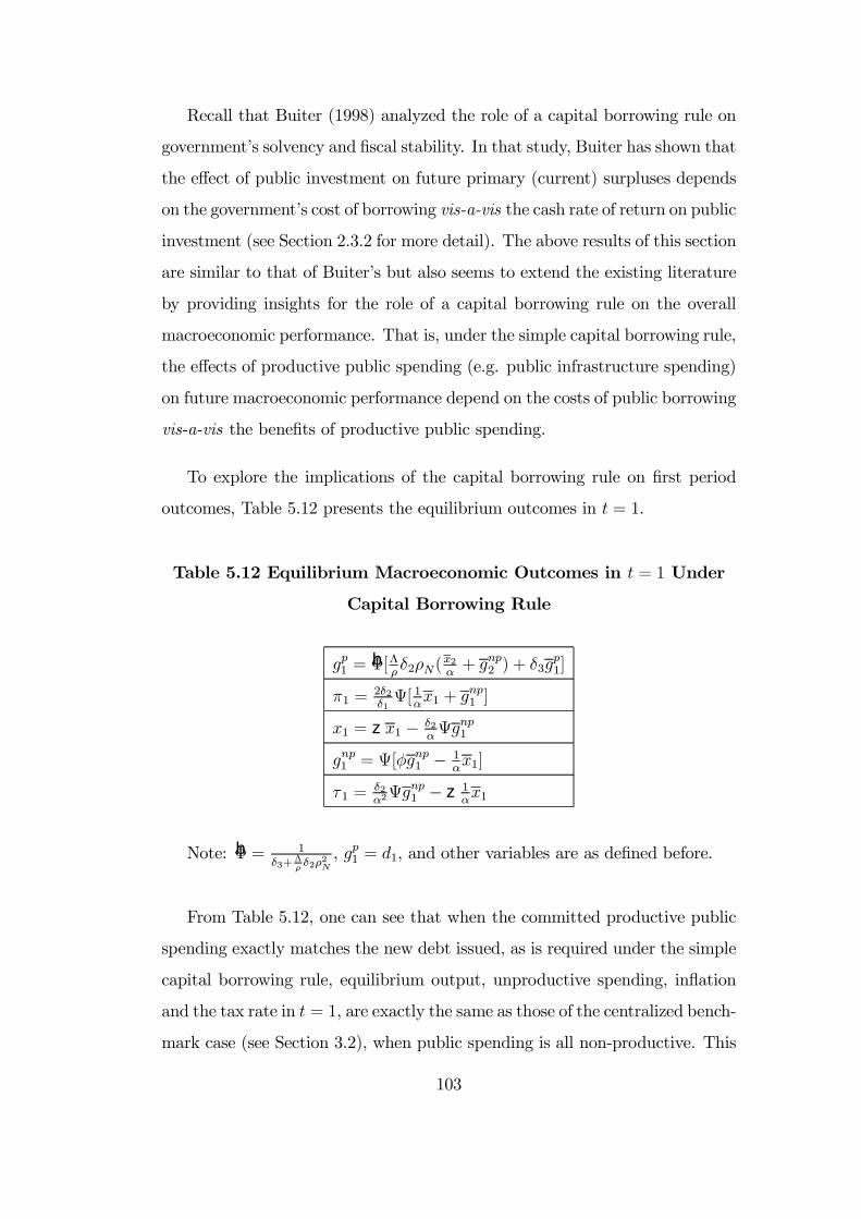
Recall that Buiter (1998) analyzed the role of a capital borrowing rule on

governments solvency and Þscal stability. In that study, Buiter has shown that

the effect of public investment on future primary (current) surpluses depends

on the governments cost of borrowing vis-a-vis the cash rate of return on public

investment (see Section 2.3.2 for more detail). The above results of this section

are similar to that of Buiters but also seems to extend the existing literature

by providing insights for the role of a capital borrowing rule on the overall

macroeconomic performance. That is, under the simple capital borrowing rule,

the effects of productive public spending (e.g. public infrastructure spending)

on future macroeconomic performance depend on the costs of public borrowing

vis-a-vis the beneÞts of productive public spending.

To explore the implications of the capital borrowing rule on Þrst period

outcomes, Table 5.12 presents the equilibrium outcomes in t = 1.

Table 5.12 Equilibrium Macroeconomic Outcomes in t = 1 Under

Capital Borrowing Rule

gp1 =bΦ[Λ

ρδ2ρN(

x2α+ gnp2 ) + δ3g

p1]

π1 =2δ2δ1Ψ[ 1

αx1 + g

np1 ]

x1 = zx1 − δ2αΨgnp1

gnp1 = Ψ[φgnp1 − 1αx1]

τ 1 =δ2α2Ψgnp1 −z 1

αx1

Note: bΦ = 1δ3+

Λρδ2ρ2N

, gp1 = d1, and other variables are as deÞned before.

From Table 5.12, one can see that when the committed productive public

spending exactly matches the new debt issued, as is required under the simple

capital borrowing rule, equilibrium output, unproductive spending, inßation

and the tax rate in t = 1, are exactly the same as those of the centralized bench-

mark case (see Section 3.2), when public spending is all non-productive. This

103

is due to the constraint that the policy maker in t = 1 could only run a budget

deÞcit equal to the amount of productive spending committed in that period;

as a result, unproductive spending is Þnanced by the tax and seigniorage rev-

enues only and thus, in effect, the balanced budget constraint still applies to

the Þnancing of non-productive spending, as noted before. Hence, the com-

parative statics for these variables are the same as those with the centralized

benchmark case (see Section 3.2.2). As expected, however, the comparative

statics of productive public spending depend on the net beneÞt of productive

spending, ρN . Table 5.13 presents the comparative statics of productive public

spending in t = 1 which can be interpreted as in the previous section.

Table 5.13 Productive Spending in t = 1: Comparative Statics

(Capital Borrowing Rule)

Case 1: ρ > 1 + r1 or (ρN > 0)

↑ x2 ↑ x1 ↑ gnp2 ↑ gnp1 ↑ gp1gp1 + 0 + 0 +

Case 2: ρ = 1 + r1 or (ρN = 0)

↑ x2 ↑ x1 ↑ gnp2 ↑ gnp1 ↑ gp1gp1 0 0 0 0 +

* gp1 = gp1

Case 3: ρ < 1 + r1 or (ρN < 0)

↑ x2 ↑ x1 ↑ gnp2 ↑ gnp1 ↑ gp1gp1 − 0 − 0 +

An interesting question relating the presence of the capital borrowing rule

is whether it would prevent strategic behavior in the making of public borrow-

ing and productive spending decisions. As mentioned before, this has indeed

104

been one of the main arguments put forward in favor of these rules. It is,

therefore, of great interest to understand how policy makers would respond to

electoral uncertainty when both the beneÞcial effects of public spending and

the detrimental effects of public borrowing fall upon uncertain future policy

makers. To this end, this section will also explore the role of electoral uncer-

tainty on an incumbent governments productive public spending and public

borrowing decisions when borrowing can only be raised to Þnance productive

public spending categories as required by the simple capital borrowing rule.

The resulting equilibrium productive public spending in the Þrst period, prior

to the elections, is as follows34

gp,E1 = bΦ∗[Λ∗ρδ2ρN(

x2α+ gnp2 ) + δ3g

p1] (5.11)


tainty, bΦ∗ = 1

δ3+Λ∗ρδ2ρ2N

, gp,E1 = dE1 , and other variables are as deÞned before.

Under the capital borrowing rule, the role of electoral uncertainty on pro-

ductive public spending is summarized by the following proposition.

Proposition 8 Under the capital borrowing rule:

i) If productive public spending does not yield intratemporal utility to the in-

cumbent government (δ3 = 0), electoral uncertainty does not affect the produc-

tive public spending in equilibrium.

ii) When productive public spending also yields intratemporal utility to the in-

cumbent government (δ3 > 0),

a) the lower (higher) the incumbents probability of re-election (p) the lower

34The same modiÞcations as in Section 4.2.1 is performed to this set-up. That is, wereplace βG with β

∗G = pβG. As the elections will take place at the end of the Þrst period,

optimal policy outcomes in the Þnal period will be the same as before.

105

(higher) the productive public spending in equilibrium if and only if ρN > 0

and

δ2(x2α+ gnp2 ) > ρNg

p1,

b) the lower (higher) the incumbents probability of re-election (p) the higher

(lower) the productive public spending in equilibrium if and only if ρN < 0,

c) the electoral uncertainty does not affect the equilibrium productive public

spending if and only if ρN = 0.

Proof. i) Provided that δ3 = 0, the derivative of gp,E1 with respect to p is

zero.

ii) Provided that δ3 > 0, the derivative of gp,E1 with respect to p is

βGDδ3ρN [δ2(x2α+ gnp2 )− ρNgp1]

(δ3 +Λ∗ρδ2ρ2N)

2

This derivative is positive if and only if ρN > 0 and δ2(x2α+ gnp2 ) > ρNg

p1.

It is zero (negative) if and only if ρN = 0 (ρN < 0).

This proposition suggest that the simple capital borrowing rule would cer-

tainly prevent strategic behavior if productive public spending does not pro-

vide utility to the incumbent government in the same period. When it does,

whether electoral uncertainty would lead to strategic behavior depends on the

sign of ρN . In other words, the capital borrowing rule may or may not prevent

the strategic use of productive public spending even when it prevents strategic

debt accumulation, as is the case here.

5.5 Conclusion

This chapter has analyzed the role of domestic public borrowing on public

spending decisions and macroeconomic performance.

106

Policy makers face an intertemporal trade-off between current and future

public spending. While borrowing raises current public spending, it lowers

resources for future public spending. As a result, it has been shown that

the higher public borrowing in the Þrst period leads to higher inßation rate,

public spending gap and output gap; hence, results in worse macroeconomic

performance in the Þnal period.

The previous chapter established that a high degree of political instability

may lead to myopic policies and associated strategic behavior in the form of

low levels of productive public spending. Similarly, this chapter has shown that

a high degree of political instability may lead to myopic behavior in another

form: excessive (strategic) debt accumulation. If the incumbent government

faces a low probability of re-election at the end of the current period, it may

accumulate excessive amount of public debt to tie the hands of its successor

by restraining the resources available for public spending in the next period.

These results (as well as those of the previous chapter) may shed some

light on Turkeys populist and myopic public spending and domestic borrow-

ing policies of the late 1980s and the early 1990s, which are associated with

unstable and polarized political environment. Furthermore, the above results

may also shed some light on the restraining effects of Turkeys domestic debt

service on public spending policies since the mid-1990s. However, it should

be noted here that the public spending and debt dynamics of the Turkish

economy over the late 1980s and the 1990s are realized under a special set of

circumstances.35 Therefore, given the simple contexts of the models of Part I,

the aforementioned results could at most provide partial explanations to the

certain aspects of the public spending and debt dynamics of the Turkish econ-

35For instance, during the 1989-1993 period, Turkey had managed to maintain the populistpolicies - through the reliance on domestic borrowing - mainly with the help of capital inßows.Moreover, as noted before, banking sector have played an important role in public borrowingpolicies as the primary buyer of the government bonds and T-bills in the shallow market.This has been the main factor behind the signiÞcant rise in real interest rates during the1990s.

107

omy during that period. This period of the Turkish economy will be analyzed

in more detail in Chapter 7.

The interesting as well as original result is that the net effect of produc-

tive spending on the next periods macroeconomic performance depends on

the beneÞts of productive public spending (ρ) relative to the costs of public

borrowing (1 + r1). For example, when the beneÞts of public spending are

exactly offset by the costs of borrowing in the next period the net beneÞt of

productive spending committed in t = 1 on macroeconomic performance in

t = 2 is zero. However, if the beneÞts of public spending are more than the

costs of borrowing in the next period, then the net effect of productive public

spending in t = 1 on macroeconomic performance in t = 2 is favorable. Pro-

ductive public spending in this case creates additional resources to (partially)

pay the costs of other forms of public spending, e.g. popular spending.

This chapter also considered the implications of a capital borrowing rule

where only public investment could be Þnanced by additional borrowing. The

obtained results suggest that even under such a borrowing rule, higher pro-

ductive public spending may yield unfavorable effects on macroeconomic per-

formance in t = 2 if the returns from investment are low, for instance, due to

low quality. In other words, qualitative as well as quantitative aspects of Þscal

management matter for macroeconomic performance. In addition, it is shown

that the capital borrowing rule does not necessarily prevent the strategic use

of public investment, even though it prevents strategic debt accumulation.

108

Part II

Macroeconomic Instability,

Capital Accumulation and

Economic Growth: The Turkish

Experience 1963-1999

109

CHAPTER 6

REVIEW OF THE LITERATURE ON THEROLE OF PUBLIC INVESTMENT ANDMACROECONOMIC INSTABILITY INCAPITAL ACCUMULATION AND

ECONOMIC GROWTH

6.1 Introduction

During the recent years, the role of public investment and macroeconomic

instability in capital formation and economic growth were among the widely

researched areas by the economists. It is, for instance, frequently argued that

the role of state1 as a provider of public investment complementary to private

investment and stable macroeconomic environment, among the other roles,2

are crucially important for sustaining growth in developing countries.

1The terms government and state will be used interchangeably throughout thisthesis.

2According to Nobel Laureate Joseph Stiglitz (1997), the governments of USA and therapidly growing East Asian countries have played six important roles in their economic devel-opment. These are: promotion of education, investment in physical and institutional infras-tructure, promotion of technology, support to Þnancial sector, prevention of environmentaldegradation and creation and provision of a social safety net. Moreover, as documentedby several studies, the role of governments have been very pivotal in East Asian countriesduring their rapid growth episodes (see, for example, Amsden, 1997 and World Bank, 1993among many others).

110

Unfortunately, Turkey and many other developing countries have experi-

enced endemic macroeconomic instability as a result of implementing unsound

economic policies over long periods of time. Consequently, most of these coun-

tries suffering from endemic macroeconomic instability tend to exhibit low

and volatile rates of private as well as public capital formation and economic

growth.

The main objective of Part II is to investigate the effects of macroeconomic

instability on public and private investment as well as on the nature of their

relationships (e.g. complementarity) and economic growth in the Turkish econ-

omy over the 1963-1999 period. As discussed in more detail in Section 1.2.1

(Chapter 1), the principal aim of this part is to extend the recent work in the

literature on the role of public capital spending in capital accumulation and

economic growth, by including the issue of macroeconomic instability and by

considering the Turkish experience. To this end, initially the present chapter

provides a selective and condensed overview of the related literature.

The rest of this chapter is organized as follows. Sections 6.2 and 6.3 review

the literatures on the role of public investment and macroeconomic instability

in capital formation and economic growth, respectively. Section 6.4 provides a

condensed overview of the Turkish evidence. Finally, Section 6.5 presents the

road map for the rest of Part II.

6.2 The Role of Public Investment in Capital

Formation and Economic Growth

In recent years, the literature on the role of public investment in capital for-

mation and economic growth has been one of the active research areas for both

developing and developed countries. Currently there are two related strands

111

of research on the role of public investment in capital accumulation and eco-

nomic growth. The Þrst one focuses on the public capital spending3-private

investment nexus. The second one analyzes the public capital spending and

output (or growth) nexus. Sections 6.2.1 and 6.2.2 provide a review of these

two strands of literature, respectively.

6.2.1 Public Capital Spending-Private Investment Nexus

Public investment is considered as one of the determinants of private invest-

ment in the public capital spending-private investment nexus literature. The

following sub-section provides the formal explanation.

Theoretical Framework

Generally speaking, in this strand of literature, public investment is included

as an explanatory variable along with other explanatory variables, such as real

output,4 in the private investment function,

Ip = f(X, Ig) (6.1)

where Ip denotes private investment, Ig denotes public investment and X

represents a set (vector) of other variables. The three conceptually different

effects of public investment on private investment can be considered depending

on the form of the relationship between public and private investment:

3The terms public investment and public capital spending are used interchangeablythroughout this thesis.

4See Agenor (2000) for a list of other determinants of private investment in the developingcountries.

112

if public investment and private investment are complementary; then, anincrease in Ig, e.g. public investment in infrastructure, increases (crowds-

in) Ip,

if Ig and Ip are substitutes; then, an increase in Ig decreases (crowds-out)Ip,

and Þnally, if Ig and Ip are unrelated ; then, an increase in Ig cannot affectIp.

Nevertheless, one should also consider the Þnancial crowding-out effect of

public investment while determining its net effect on private investment. That

is, an increase in public investment may lead to a reduction in private invest-

ment due to the unfavorable effects of government Þnancing (e.g. borrowing)

on the existing Þnancial resources and/or on the interest rates.5 Therefore,

both effects of public capital spending should be considered for a meaningful

policy making.

Empirical Results

This section provides a selective overview of the empirical results in the public

capital spending-private investment nexus literature, due to the existence of

a vast research since the early 1980s. The analysis is performed under two

headings: multi-country studies and country-speciÞc studies.6

5Along the neoclassical lines, traditional crowding-out hypothesis states that an in-crease in public investment results in equal fall in private investment due to the effect ofgovernment borrowing (for Þnancing its expenditure) on interest rate. This is full orcomplete Þnancial crowding-out effect. However, an increase in public investment does notnecessarily lead to full Þnancial crowding-out effect. Its magnitude depends on the structureof economy (e.g. structure of the Þnancial system).

6While the Þrst group of studies are based on cross-section or panel data, the secondgroup of studies are based on a single-country time series data.

113

Multi-Country Studies

One of the seminal studies in this literature is by Blejer and Khan (1984).

This study attempted, for the Þrst time, to analyze the effects of both in-

frastructural and non-infrastructural components of government expenditure

on private investment. It is this characteristic which distinguishes this study

from early studies (see, Blejer and Khan, 1984, for more detail on these earlier

studies).

Their model on private investment is a variant of the ßexible accelerator

model which incorporates roles for both Þscal and monetary policies. And they

estimated four different versions from pooled data on 24 developing countries.

The infrastructural component has positive and signiÞcant value and the op-

posite is true for non-infrastructural component. This means that there is

a signiÞcant crowding-in effect of infrastructural component. These results

conÞrmed the a priori expectations.7 They have also emphasized that if es-

timation is done without distinguishing infrastructural component from non-

infrastructural component, the results could be insigniÞcant, as it is reported

in their regressions and in many other cited studies (see, Blejer and Khan

1984).

Blejer and Khan (1984) explicitly state that the government should be

careful in its decision on the components of public expenditure since it may

either have positive (crowding-in) or negative effects (crowding-out).

More recent multi-country studies used panel data in their analyses. Car-

dosa (1993), for example, analyzed private investment in six Latin American

Countries (LACs)8 by using a regression analysis on quadrennial panel data

7However, the magnitudes of the coefficients are quite different. This is due to thefact that different approaches for calculating proxies (e.g. for infrastructural and non-infrastructural components) will result in different values, in different estimation results.This is explicitly emphasized by Blejer and Khan in their conclusion. See Blejer and Khan(1984) for more detail.

8These are : Argentina, Brazil, Chile, Colombia, Mexico and Venezuela. They representmore than 85% of all LACs GDP.

114

for the 1970-85 period. Cardosa noted the complementarity between private

and public investment and found that [in]... regressions a one-percentage

point increase in the share of public investment in GDP raises the share of

private investment in GDP by more than a half percentage point (Cardosa,

1993: 845). She further noted that [t]his complementarity does not rule

out the possibility that an increase in the budget deÞcit crowds out private

investment (Cardosa, 1993: 845) and found crowding-out effect but with in-

signiÞcant coefficients. Due to this reason, Cardosa suggested tax-Þnancing

instead of domestic-debt Þnancing. Moreover, Cardosa blamed the decline in

private investment shares during the 1980s on a reduction in complementary

public investment in LACs, as well as on other causes, such as macroeconomic

instability.

A study by Argimon et al. (1997) investigates the relationship between gov-

ernment spending and private investment on a panel data of 14 industrialized

OECD countries9 for the period 1979-1988. Their empirical results lend sup-

port to a crowding-in effect of infrastructure investment on private investment.

Furthermore, while they found no considerable evidence on direct crowding-

out of public investment, they found considerable evidence on crowding-out

effect of public consumption.

A study by Ahmed and Miller (1997) examined the effects of disaggregated

government expenditure namely, defense, education, health, social security and

welfare, transportation and communication, on total investment (39 countries

over the 1975-84 period).10 They used Þxed-effect and random-effect (panel

data) methods for investigating tax-Þnanced and debt-Þnanced government

9See Argimon et al. (1997: 1004, footnote no. 3) for the list of countries included in thatstudy.10Ahmed and Millers study is quite different from the previous studies cited in this Sec-

tion. Firstly, as mentioned above, their disaggregation of public expenditure is more speciÞccompared to the previous studies. Secondly, they incorporated the government constraintinto the regression equations; in order to analyze the effects of tax-Þnanced and debt-Þnancedgovernment expenditure on investment. These two characteristics of the study are very im-portant for the more sensitive and meaningful analysis of the government expenditures oninvestment.

115

expenditure for the samples of developing and developed countries, and also

for the full sample of both groups.11 They found that expenditure on social

security and welfare crowds-out domestic investment in all samples. Another

important result from this study is that expenditure on transportation and

communication crowds-in investment in developing countries but not in devel-

oped countries. Ahmed and Miller stated that:

[o]ne possible explanation for this Þnding is that developing coun-

tries have not yet reached the threshold where further government ex-

penditure on transportation and communication no longer adds to pro-

ductivity and thus no longer encourages private investment. In contrast,

developed countries have passed this threshold level (Ahmed and Miller,

1997: 8).

Agenor (2000) provides more evidence on the recent multi-country studies

on developing countries.

Country-SpeciÞc Studies

USA

Aschauer (1989b) by using a neo-classical framework has investigated the

effects of public capital spending on private investment.12 Aschauer conducted

his study on USA times series data (1953-86). He found that direct crowding-

out effect of non-military public capital investment on private investment is

outweighed by the (indirect) crowding-in effect; that is in his study the net

effect is in favor of crowding-in effect. Consequently, Aschauer underlined the

11See Ahmed and Miller (1997: 5, footnote no.3) for more detail on the countries includedin these samples.12As noted before, one of the earlier studies in the crowding-in, or more broadly, public-

private investment nexus literature is the work of Blejer and Khan (1984); however, thisliterature has exploded with the pioneering work of Aschauer [Aschauer (1989b)].

116

importance of decomposing overall public expenditure into various categories

and that it is inadequate to consider only the overall level of government ex-

penditure. He emphasized the importance of this decomposition by giving an

example:

it should not be supposed that a decision to cut $50 billion from the

defense budget and shift the funds to highway construction will have no

effect on the economy, despite the fact that total government outlays

are left unaltered. While this statement makes common sense, it is

not reßected in current macroeconomic modelling practice (Aschauer,

1989b: 185-6).

Erenburg (1993) tried to test the neutrality proposition13 of the Rational

Expectation School of thought, by using an econometric technique on the USA

data over the 1947-1985 period. He stated that the previous studies either

failed to validate or refute the neutrality proposition since they only focused

on the demand-side of the public expenditure and not on the supply-side.

Erenburg (1993) found a signiÞcant positive relationship between public and

private investment and emphasized the importance of the decomposition of

overall public expenditure. Erenburg (1993) stated that:

[i]f government provision of public capital enhances the marginal ef-

Þciency of private investment, the government sector investment should

be viewed as an indirect subsidy to the private sector via infrastructure

Erenburg (1993: 836).

Cote dIvoire

13According to this proposition: unexpected (expected) government policy has (no) per-manent effect on output.

117

During the 1980s, Cote dIvoire experienced a severe and long lasting Þnan-

cial and economic crisis. As a result, the Ivorian governments had resorted to

successive structural adjustment programs. The major component of these pro-

grams was Þscal adjustment entailing public spending cuts, especially in public

investment. However, Kouassy and Bohoun (1994) found a net crowding-in ef-

fect of public investment14 on private investment by using a speciÞc15 growth

model. They also performed simulations of alternative policies and found that

the best suited policy lowers Þscal deÞcit and at the same time preserves the

growth; for example, an increase in public investment can be accompanied by

cuts in government consumption.

Some Other Developing Countries

In Taylor (1993),16 the following simpliÞed private investment equation

is estimated by the country papers authors of this study:17 Ip = Io+αIg+βu

, where Ip and Ig are private and public investments normalized by potential

output, respectively and u denotes the capacity utilization rate, i.e. u = actual

output / potential output. Coefficient α captures crowding-in or crowding-out

effect: if it is negative (positive) there is a crowding-out (crowding-in) effect.18

Coefficient β is used to capture an accelerator effect and Io denotes the constant

term. With the exception of the two countries, Chile and Colombia, values

for α are positive and it ranges from -0.4 (Colombia) to 1.6 (Malaysia). For

Turkey, the value of α is 0.185; that is, there is a crowding-in effect.19 This

result will be analyzed in more detail in Section 6.4.

14They stated that there is a need for further disaggregation of public investment intoinfrastructural and non-infrastructural components since this would shed more light on thelocation of positive effects of public investment (Kouassy and Bohoun, 1994: 1125).15See Kouassy and Bohoun (1994: 1120-3).16Bacha (1990) and Taylor (1991) incorporated the crowding-in effect into the three gap

analysis.17See Taylor (1993) for additional information.18Taylors (1991) private investment equation is somewhat less restrictive than this one.

See Taylor (1991) for more detail.19See Taylor (1993: 28, Table 2.3) for additional information on α coefficient in other

countries and β coefficient in all countries in the sample.

118

Agenor and Montiel (1996)20 provides an overview of earlier studies on

developing countries in this strand of literature. However, there are certain

common problems, such as endogeneity and spuriousness of the results, in the

early studies of this (as well as the other strand of) literature. These problems

will be considered in Section 6.2.2.

Overall, the selective evidence (both from country-speciÞc andmulti-country

studies) reported in this section lends support to the complementarity between

public investment (especially in infrastructure) and private investment. How-

ever, early studies (reported in Agenor and Montiel, 1996 and Blejer and Khan,

1984) provided mixed results. The evidence on the Turkish economy is also

ambiguous (see Section 6.4).

6.2.2 Public Spending-Output (Growth) Nexus

There are at least two channels through which public spending may affect the

rate of economic growth. A rise in public spending, e.g. public investment,

leads to an increase in capital stock; thus, output. Similarly, a rise in produc-

tive public spending, such as spending on education, health and infrastructure,

raises overall productivity (as well as marginal productivity of privately owned

inputs) and hence output. These mechanisms will be more formally considered

below.

Theoretical Frameworks

Generally speaking, the role of public capital spending in economic growth

can be theoretically analyzed both in a simple production function framework

(Aschauer, 1989a) and in a new growth theory framework (Barro, 1990).

Barro (1990) is one of the seminal works in a new growth theory frame-

work. Barros model links government expenditure on infrastructure, which

20See also Blejer and Khan (1984).

119

is assumed to be complementary to private investment, to the growth pro-

cess. In this model, Þrms production functions include both private capital

input and publicly provided capital (infrastructure).21 It is assumed that gov-

ernment maintains Þxed proportion of public expenditure to output, which

is totally Þnanced by income tax due to balanced budget assumption. The

main idea of this model is that when individual Þrms increase their production

they increase overall output and income, thus, revenues of the government,

which implies higher infrastructure and higher productivity for other Þrms.

This is the externality effect of higher infrastructure. However, it should be

mentioned that there is no direct government intervention to the economy,

since there is a built-in process for the determination of public infrastructure.

Furthermore, an increase in public infrastructure also has negative effects on

growth, because it is Þnanced by distortionary income tax that negatively af-

fects the marginal productivity of capital. Therefore, Barro (1990) calculates

the optimal tax rate which maximizes long run growth rate of the economy.22

However, Barros (1990) model is not suitable for analyzing the effect of govern-

ment spending in developing countries. Such balanced budget assumption is

not plausible for developing countries as it is for developed countries. Accord-

ing to Strauss (1998), this is one of the drawbacks of the Barros (1990) model

since the governments taxation ability is limited in most developing countries.

Furthermore, governments in many developing countries increasingly rely on

seigniorage and public borrowing to Þnance their spending.

Besides Barros (1990) model, there are other endogenous growth models

on the role of public spending in economic growth.23 More recently, David

Aschauer has also worked with endogenous growth models (Aschauer, 1998).

He examined the effects of different means of Þnancing government expenditure

on growth and inßation within an endogenous growth setting. One of his

21See Agenor (2000) for a simpliÞed exposition of this model.22It is equal to natural efficiency condition of the size of the government (Barro, 1990).23See Agenor (2000) for additional models on the role of public spending (including capital

spending) in economic growth.

120

main Þndings is that optimal public Þnance requires productive government

expenditure to be Þnanced by money creation and unproductive government

expenditure by income taxation (Aschauer, 1998: 1).

A widely used theoretical framework is the production function approach.

In this framework public capital can be considered as a factor inßuencing total

factor productivity and/or as an additional input in the production function.

More formally,24

Y = A(Kg)F (Kp,Kg, L) (6.2)

where Y is the real output of private sector, A is the total factor productiv-

ity, L is the level of employment, Kp and Kg denote private and public capital

stocks, respectively.25

In practice, the following neoclassical production function framework is

widely used to analyze the effects of a rise in public investment (or Kg) on

output:

Y = F (L,Kp, Kg) + Zy (6.3)

F1, F2 > 0, F11, F22 < 0, F12 > 0

F3 > 0, F13 > 0, F23 ⇔ 0

where Zy is a shift parameter of production function (e.g. related to the

technology) and all the other variables are as deÞned before.

24A related but somewhat different approach is the growth accounting or sources of growthanalysis. This approach also uses production function but public capital is not included asan input. See Sturm et al. (1998: 7) for more detail.25It should be noted that production function approach is criticized on theoretical grounds.

For example, it is claimed that production function framework is inappropriate for analyzingthe long run effects of public capital spending. (see, for example, Pereira, 2000; and Mittnikand Neumann, 2001 and the references therein).

121

In this framework, three conceptually different effects of an increase in

public capital stock (Kg) on real output (Y ) can be identiÞed based on the

relationship between Kp and Kg:

(Case I) Kp and Kg are complementary: An increase inKg will directly

increase Y (F3 > 0) and indirectly increase Kp and Y via increasing the

marginal productivity of Kp (F23 > 0). It will also indirectly increase Y

by raising the marginal productivity of L via increasing the availability

of Kp and Kg per worker (F12 , F13 > 0). Overall, an increase in Kg will

deÞnitely increase Y .

(Case II) Kp and Kg are substitutes: An increase in Kg will directly

increase Y but it will also indirectly decrease Y (F23 < 0); therefore the

net effect on Y is uncertain. Y will decrease when the following condition

holds: [(F3 + F13) + (F23 − F12)] < 0.

(Case III) Kp and Kg are independent: An increase inKg will (directly)

increase Y but it will not affect Kp (F23 = 0).

Empirical Results

The empirical results in this strand of the literature is also vast and expanding.

Therefore, this section will provide a selective overview. However, in line with

the aim of Part II, this section will pay more attention to the country-speciÞc

time series analysis. Therefore, a summary of multi-country empirical analysis

will be provided Þrst.26 Then, a review on the country-speciÞc studies will be

provided.

26According to Sturm et al. (1998), there are Þve ways of modelling government spend-ing and economic growth at a macro level. These are: 1) production function approach,2) behavioral approach, 3)VAR approach, 4)Barro-type (cross-section) regressions and 5)structural models. Sturm et al. comprehensively reviewed the literature and providedpros and cons of the Þve different approaches. However, it should be mentioned here thatSturm et al.s classiÞcation is quite arbitrary since it includes both theoretical and empiricalapproaches.

122


Cross-section empirical studies are widely used in the multi-country anal-

ysis. Most of the empirical work related to the endogenous growth theory

are comprised of Barro-type cross-section regressions.27 Even though many

studies have found positive effect of public investment on growth, the overall

evidence is mixed (Agenor, 2000).28 However, as indicated in Chapter 2, the

favorable role of public infrastructure investment in economic growth is widely

shared by many economists. For example, Easterly and Rebelo stated that

investment in transport and communication is consistently correlated with

growth (Easterly and Rebelo, 1993: 417). They also argue that the causality

runs from public investment to growth rather than the other way round. By

doing a cross-section regression analysis on developing countries, they found a

high correlation (between .59 and .66) between transport and communication

investment and per capita growth rate. Nevertheless, these cross-section stud-

ies were criticized on empirical grounds such as omitted variable, endogeneity

and fragility (Munnel, 1992 and Sturm et al., 1998).29

Furthermore, cross-country analyses are also criticized by both develop-

ment economists and macroeconomists since they are based on representa-

tive and/or average developing country assumption (see Temple, 1999: 150

and the references therein). That is, heterogeneity is an important factor for

the developing countries; hence, country-speciÞc empirical work on some issues

may provide better insights into the analysis of economic growth (Gani, 1998

and Ericsson et al., 2001). In this respect, time series (econometric) analysis

27In this (empirical) approach public investment is added to the regression analysis asan explanatory variable. See, for instance, Barro (1989, 1991). Also see Levine and Renelt(1992) for a careful review of cross-section growth regressions.28See Sturm et al. (1998) for the references of the other studies.29Omitted variable issue (problem) arises when a relevant variable is excluded from the

empirical model. Endogeneity problem occurs, for example, when an endogenous variable istreated as an exogenous variable. Fragility occurs when estimate of the coefficient of a keyvariable signiÞcantly changes with the inclusion or exclusion of one or more other variable(s).See Munnel (1992) and Sturm et al. (1998) for more detail.

123

has become very important.30


USA

Aschauer in his seminal work (Aschauer, 1989a) utilized a production func-

tion approach. He found that a core infrastructure (highways, airports, mass

transit, street etc.) has strong explanatory power for productivity in United

States. Aschauer estimated the elasticity for the core infrastructure, which ac-

counted for 55% of non-military capital stock during 1949-85, as .24 (Aschauer,

1989a: 193). He also found a strong positive relationship between average an-

nual labor productivity and public investment-gross domestic output ratios for

the period 1973-85 for G-7 countries (see Section 2.2).

Nevertheless, Aschauer and others31 obtained an estimate for the marginal

productivity of public capital32 between -0.11 and 0.54. These results are

criticized to be controversial results since the range of estimates were found to

be large. Furthermore, Aschauers results were considered to be very high by

the critiques (Sturm et al., 1998; and Aschauer, 1998).

There are also certain common problems in the early application of this

approach with the single equation regression: the reverse causality (between

Y and Kg), endogeneity (of Kg), and spuriousness of the results (i.e. due to

the inclusion of stationary and non-stationary variables in the same empiri-

cal model).33 Nevertheless, during the recent years many studies by utilizing

modern time series techniques, such as vector autoregressions, have addressed

30Recent progress in panel data techniques are also encouraging for growth studies (Tem-ple, 1999).31See Sturm et al. (1998) for the references.32Aschauer used a Cobb Douglas production of the form: Y = A Kα

pKβg L

ϕ, where βrepresents the marginal productivity of public capital.33As it is rightfully emphasized in modern econometrics and time series econometrics, it is

crucially important to consider the time-series properties of variables for obtaining sensibleresults. See, for example, Johnston and Dinardo (1997) and Franses (1998) for more detail.

124

these empirical critiques and found supportive empirical evidence on the favor-

able effects of public capital spending on private capital formation and output.

These studies will be analyzed in more detail at the end of the current section.

Mexico

Ramirez (1998) has tried to deal with some of the above critiques in his

study. He employed the following modiÞed neoclassical production function:

Y = F (L,Kp, Kg,X) + Zy (6.4)

where X represents a set (vector) of variables that early researchers in-

cluded in the production function to explain the real output level (e.g. domes-

tic credit to private sector, level of exports)34 and all the other variables are

as deÞned before. As mentioned above there are three conceptually different

effects of an increase inKg on Y depending on the form of relationship between

Kp and Kg.

Since most of the developing countries lack consistent estimates for both

private and public capital stock the direct estimation of equation (6.4) is not

possible. However, researchers have overcome this problem by estimating the

production function in the growth rate form. Therefore, percentage change in

public (private) investment can be used as a proxy for the percentage change

in public (private) capital stock.35 Ramirez (1998) estimated the growth rate-

form of the equation (6.4) as a productivity growth36 relationship for Mexico

over the 1950-1990 period. In order to overcome the reverse-causation critique

he used instrumental variable (IV) estimates. He also checked for cointegration

and found one cointegration relation. In sum, Ramirez found that both public

34See Ramirez (1998) for more detail.35Or, alternatively, ratio of public (private) investment to output can be used.36Ramirez obtained the Þgures for productivity growth by subtracting the percentage

change in economically active population from the growth rate of output.

125

investment and private investment have signiÞcant effect on output.37

Cameroon

Ghura(1997) analyzed the factors affecting economic growth in Cameroon

during the 1963-96 period. He modiÞed the Solow-Swan production function

by following the implications of several endogenous growth models, which em-

phasize the importance of the roles of public and human capital in economic

growth (Barro, 1990; and Lucas, 1988). More formally, Ghura employed the

following production function,

Y = AKαpK

βg Z

γ (6.5)

where Z = HL, H represents human capital development, and all the other

variables are as deÞned before.

Thus, Ghura modiÞed the Solow-Swan production function by incorporat-

ing Kg and H. By referring to equation (6.5), he noted that if we assume

α + β + γ > 1 (increasing returns to scale), endogenous type models are able

to generate sustained growth from the factors endogenous to the economic

system like human and physical capital accumulation via externalities. As in

the analysis of Ramirez (1998), lack of consistent estimates for both private

and public capital stock for Cameroon led Ghura to estimate the growth rate

form of the above production function.38

He found that the estimated aggregate production function for the Cameroon

exhibits increasing returns to scale. Furthermore, increases in private in-

vestment, public investment, respectively increases economic growth rate of

37In other study, Nazmi and Ramirez (1997) analyzed the impact of public and privateinvestment expenditures on growth rate of Mexican economy (over the 1950-1990 period)by using simultaneous equation model. They found a positive effect of public as well asprivate investment on output. However, they noted a signiÞcant crowding-out effect ofpublic investment on private investment.38Compared to Ramirez, Ghura used slightly different forms of proxy by making some

assumptions. See Ghura (1997) for more detail.

126

Cameroon. Moreover, a progress in human developments, also contributes to

economic growth. Prudent Þscal stance and economic policies aimed at increas-

ing external competitiveness also help to spur growth.39 Overall, according to

Ghura, these results support endogenous-type growth model for Cameroon.

Country-SpeciÞc Studies Based on Vector Autoregressions (VARs)

The above recent studies, which are based on a single-equation analysis

(Ramirez, 1998; and Ghura, 1997), have addressed some of the aforemen-

tioned empirical critiques (e.g. spuriousness) but not all (e.g. reverse causa-

tion). Fortunately, vector autoregression approach to the empirical modelling

is a relatively less restricted approach with respect to the problems of reverse

causation, endogeneity and time series properties of the data.40 That is, the

VAR approach is more data oriented and all variables are treated as jointly

determined.

More recent studies utilized other modern multivariate time series tech-

niques such as cointegration and impulse response analyses within the VAR

framework. For example, cointegrated VAR (or vector error correction, VEC)

models are more promising way for grasping and interpreting the relationships

between public investment, private investment and output since they allow

the determination of both short-run (as well as medium-run) dynamics and

long-run relationships within the same framework.41 The importance of this

ßexibility with respect to short and long-run analyses is noted by Glomn and

Ravikumar (1997: 199): Þnding small short-run effects does not imply that

public capital has no (long-run permanent) effect.42

39He analyzed this by adding relevant variables to the empirical counterpart of the equa-tion (6.5), see Ghura(1997) for more detail.40See Sturm et al.(1998) for an overview of the pros and cons of this approach as well as

a review of the earlier studies conducted with this approach.41Economic theory plays two important roles in the development (or empirical speciÞca-

tion) of error-correction models: 1) it suggests explanatory variables to be included and 2)it identiÞes the long-run relations between variables (Kennedy, 1998:267). See Section 8.2for more detail.42Sometimes it takes 5-10 years to see the effects of public infrastructure investments. See

Glomn and Ravikumar (1997) for references.

127

Ghali (1998), for example, by utilizing multivariate cointegration tech-

niques, developed a vector error-correction (VEC) model43 of growth to ana-

lyze the long-run effects of public investment (Ig) on private investment (Ip)

and output (Y ) in Tunisia over the 1963-93 period. Ghali referred to the

neoclassical production function (equation (6.3)) in order to provide implica-

tions for the relationship between Ig and Ip from the relationship between Kp

and Kg (as explained above).44 Ghali used the Johansen Cointegration tech-

nique for testing and estimating long-run relationship for the three variables

(Ip, Ig, Y ), and then (after Þnding one cointegration relationship)45 formed

vector error-correction (VEC) model of growth with these variables and an-

alyzed the dynamics of the public-private capital formation in Tunisia. He

found that public investment is having a negative short-run impact on pri-

vate investment and a negative long-run impact on both private investment

and economic growth (Ghali, 1998: 837).46

Ghali (1998) used his reported short-run coefficients (from the VEC model)

and the results of the Granger-causality tests in his evaluation of the short-

term dynamics and the resultant implications. However, Kulshreshtha and

Nag (2000) criticized Ghalis (1998) study for being inadequate on method-

ological grounds, especially on the analysis of short-term dynamics. As a

result, they stated that authors conclusion on short-term dynamics should

be treated by caution.47 Moreover, by referring to Pesaran and Shin (1998),

they suggested that [t]he plausible structures or short-run dynamics could be

43See Sturm et al.(1998) and Glomn and Ravikumar (1997) for the results of the earlystudies under this approach, i.e. VEC framework.44However, it should be noted here that Ghali implicitly assumed that Ig and Ip are the

proxies for Kp and Kg, respectively, but this does not seem to be valid, at least in theproduction approach framework (see Ramirez, 1998; and Ghura, 1997).45This long-run relationship is: Y = −1.7Ig+2Ip. He found a positive (negative) effect of

Ip(Ig) on Y .46Similarly, Ghali and Al-Shamsi (1997) have formed VEC model for United Arab Emi-

rates to analyze the role of Þscal policy in economic growth process. Their analysis lendsupport to the importance of decomposition of public spending. That is they found positive(negative) effect of an increase in public investment (consumption) on economic growth.47See Kulshreshtha and Nag (2000) for more detail.

128

studied by innovation accounting tools such as impulse responses and error

variance decompositions (Kulshreshtha and Nag, 2000: 582).

More recently, Pereira (2000) and Mittnik and Neumann (2001), by utiliz-

ing innovation accounting tools, found positive effects of public capital spend-

ing on private investment and output. Pereira (2000), for example, investi-

gated the effects of public investment on private sectors output in the USA

(1956-1997) by using a VAR approach. He found that all types of public invest-

ment, including total as well as core infrastructure investments, have positive

(crowding-in) effects on private investment and output. Similarly, Mittnik and

Neumann analyzed the effects of total public investment on private investment

and output by examining the impulse responses derived from the cointegrated

VAR models, which are estimated by using the data from six industrial coun-

tries.48 One of their main Þndings is that there is a strong evidence for com-

plementarity between public and private investment. Furthermore, they found

a positive effect of public investment on output.

6.3 The Role of Macroeconomic Instability in

Capital Accumulation and Growth

Inßation rate is usually utilized as the proxy measure of macroeconomic in-

stability. For instance, according to Fischer (1993b: 487), inßation rate is the

best single indicator and serve as an overall ability of government to manage

the economy. Nevertheless, a rise in macroeconomic instability means a rise

in one or more policy-induced macroeconomic instability indicators, such as

public deÞcit to GNP ratio, external debt to GNP ratio, as well as inßation

rate. This deÞnition is in line with Fischer (1993a,1993b) and Bleaney (1996)

48These are: Canada, France, UK, Japan, Germany and the Netherlands. See Mittnikand Neumann (2001) for more detail on the data period.

129

among many others, and will be used throughout this study.49

It is commonly shared by many economists that macroeconomic instability

is detrimental to economic growth (Kormendi and Meguire, 1985; Fischer,

1993a, 1993b; and Bleaney, 1996).50 Moreover, many economists believe that

chronic macroeconomic instability may lead to a low level of foreign direct

investment, worsening of income distribution and poverty.

There are a variety of channels through which macroeconomic instability

may affect the rates of capital formation and economic growth. These channels

will be explained in Section 6.3.1 below. Then, Section 6.3.2 provides the

review of the related empirical evidence.

6.3.1 Theoretical arguments

Theoretical arguments in this line of research focused on the detrimental ef-

fects of macroeconomic instability on private investment and productivity;

thus on economic growth. For instance, it is widely argued that macroeco-

nomic instability adversely affects the rates of productivity and investment

mainly by creating uncertainty about current and future macroeconomic en-

vironment. More formally, a rise in the level of macroeconomic instability, i.e.

an increase in inßation (and its variability),51 via creating macroeconomic un-

certainty and distorting information, would adversely affect economic growth

at least through the following mechanisms (Fischer, 1993b and Agenor, 2000):

uncertainty reduces the efficiency of price system, which will in turnreduce both the level and the rate of productivity,

49Consistent with this deÞnition, macroeconomic instability index is developed in the nextchapter for empirical purposes.50World Bank (1993), for example, argued that stable and sensible macroeconomic policies

promoted the economic growth in East Asian Countries.51Empirically, it is true that a rise in the level of inßation also rises its variablity and its

predictability. See Romer (2001: 522) for an overview and for evidence.

130

temporary uncertainty also reduces the rate of private investment, bygenerating option value of waiting,52 i.e. potential investors wait for

resolution before committing themselves (Fischer, 1993b), and reducing

expected proÞt,53

uncertainty increases capital ßight and this lowers capital accumulation.

Nevertheless, these channels are more relevant to private investment and

productivity. Macroeconomic instability may also have negative effects on

public investment but via different channels. While a rise in macroeconomic

uncertainty is the main cause of a reduction in private investment, the re-

duction in the Þscal (as well as political) ability of the government is the

principal reason for the decrease in public investment. That is, a rise in the

level of macroeconomic instability leads to (or aggravates) Þscal stringency

due to the existence of the budget constraint of the government. For example,

high inßation rate and/or excessive debt accumulation lowers the overall pub-

lic resources otherwise available for public expenditures, namely capital and

current expenditures, at least through the following channels:

On the one hand, a rise in inßation rate usually raises the degree ofdollarization and results in a loss of seigniorage revenue, by reducing the

demand for domestic currency.

Furthermore, high inßation rate also lowers the revenues from ordinary

taxes due to the Olivera-Tanzi effect.

On the other hand, high indebtedness leads to a high debt burden (prin-cipal plus interest payment) and lowers the overall public resources avail-

able for other public expenditures, including public investment.

52See Fischer (1993b: 486-90) for more detail and the references.53See Agenor (2000) for more detail.

131

Hence, a rise in the level of macroeconomic instability or the existence of

chronic instability lowers the public resources via these channels. In turn,

the incumbent government lowers public capital expenditures rather than cur-

rent expenditures when she is faced with Þscal stringency since it is politically

easier to cut the former than the latter (Roubini and Sachs, 1989b). This

view is widely shared by many economists and there is empirical evidence that

supports it.54 Moreover, in the case of politically unstable and polarized envi-

ronment, there are more incentives for the incumbent government to cut public

investment rather than current spending (see Chapter 2 for an overview of the

effects of political instability and polarization on public spending decisions and

related empirical evidence).

Given the detrimental effects of macroeconomic instability on public invest-

ment, there seems to be an additional (albeit indirect) link between macroe-

conomic instability and economic growth due to the possible complementarity

between public and private investment. Thus, macroeconomic instability can

be very costly in terms of private capital accumulation and hence economic

growth if public and private investment are complementary.

Quite recently, the role of exchange rate variability on investment has drawn

the attention of the economic policy makers as well as researchers.55 For ex-

ample, it is argued that a rise in the exchange rate variability, by creating

uncertainty, may lead to a fall in the level of investment (see, for instance,

Byrne and Davis, 2003, for an overview of the relevant literature and for em-

pirical evidence). Exchange rate variability may also lead to a high degree

of dollarization and hence result in a loss of seigniorage revenue (see Agenor,

54See, for example, De Haan et al. (1996) for an overview and empirical evidence.55Early studies on the role of macroeconomic stability in capital accumulation have also

noted the importance of sensible and stable exchange rate policies. For example, Fischer(1993a) pointed out that exchange rate overvaluations would harm the economy. He sug-gested that the black market exchange rate premium can be used as a proxy indicator.However, he also indicated that external debt to GNP ratio could be used as an indicatorof the exchange rate overvaluation(s) (Fischer, 1993a: 14).

132

2000, for more detail. Also see Bahmani-Oskooee and Domac, 2002, for the

Turkish experience).

6.3.2 Empirical Evidence

This section selectively reviews the empirical evidence on the role of macroe-

conomic instability in capital formation and growth. An overview of multi-

country empirical analysis will be provided Þrst. Then, a review on the

country-speciÞc studies will be provided.


Fischer (1993a) conducted cross-section analysis over the 1970-85 period

and provided case studies for Cote dIvoire and Chile to analyze the role of

macroeconomic instability in economic growth. Conclusion of his study is,

[p]rovided that inßation rate, external debt, and government deÞcit

are accepted as macroeconomic policy indicators, both the cross-sectional

regressions and the case studies support ... that a countrys macroeco-

nomic policy matter for long-run growth (Fischer, 1993a: 32).56

Bleaney (1996) provided additional cross-section (1980-90) evidence for de-

veloping countries which supported the earlier studies. His conclusion is that a

good macroeconomic management (or macroeconomic stability) is associated

with higher rate of economic growth, for a given level of investment. However,

he noted that [i]t is less clear that the volume of investment is signiÞcantly

affected (Bleaney, 1996: 461).57

56Similarly, Fischer (1993b) used a regression analog of growth accounting, which is aproduction function based approach, in his other analysis. His conclusion is the same.57It should be noted here that those critiques on the cross-section studies mentioned in the

previous sections (omitted variable, endogeneity and fragility) are also applicable to theabove studies. Recall that representative and/or average developing country assumptionof cross-section studies is also criticized.

133

Cardosa (1993)58 found some evidence of negative effect of economic insta-

bility59 on private investment in Latin America, by using a regression analysis

on quadrennial panel data for the 1970-85 period.


Spain

The Sanchez-Robles (1998) study appears to be the Þrst study that has used

the cointegration technique for studying macroeconomic stability and growth

(with the exception of the studies on inßation and growth).60 According to

Sanchez-Robles (1998), the degree of macroeconomic stability in a country

is not an easily quantiÞable concept; Fischer (1993[b]) selects some indicators

(inßation rate, public deÞcit...) that could be used as proxies of instability

in the empirical analysis (Sanchez-Robles, 1998: 587). Sanchez-Robles em-

ployed single-equation cointegration analysis for Spain for the 1962-95 period,

by using per capita income growth rate as dependent variable and has used

each of the proxies for instability separately as a regressor, including constant

and investment-to-income ratio, in various estimations. By treating these esti-

mation results as empirical regularities, he concluded that macroeconomic sta-

bility should be regarded as a prerequisite for economic growth in the Spanish

economy.

USA

Paul and Biswal (1998) investigated the various direct and indirect routes

between macroeconomic factors, including the proxies, such as budget deÞcit

and inßation, identiÞed by Fischer (1993b), and economic growth by using

VAR technique with the quarterly USA data (1967-1991). They found that the

conventional macroeconomic variables (including Fischers proxies), compared

58See the previous section for more detail.59For this purpose Cardosa developed a simple index of stability by simply adding the

log of (1 + inßation rate), log of debt ratio and log of the coefficient of variation of realexchange rate (Cardosa, 1993: 843).60See Briault (1995) for an overview.

134

to the variables identiÞed by the endogenous growth theory, seems to have

greater effect on the economic growth rate of US economy.

Developing Countries

Agenor (2000) provides additional supporting evidence for developing coun-

tries.61

Finally, it is worthwhile to note that the above mentioned empirical studies,

which assessed the effects of macroeconomic instability on investment, either

used aggregate investment (see, for example, Bleaney, 1996) or private invest-

ment data (see, for example, Cardosa, 1993) in their analyses. In other words,

those studies assessed the effects of macroeconomic instability on private or

total investment but not public investment. This issue will be considered in

more detail in Chapter 8.

6.4 Turkish Evidence: An Overview

This section provides a condensed and selective overview of the recent Turkish

evidence on the role of public investment and macroeconomic instability in

capital formation and economic growth.

The evidence on the nature of the relationship between public investment

and private investment is ambiguous in the Turkish economy (see, for example,

Anand et al., 1990; Boratav and Turel, 1993; Celasun and Tansel, 1993; Con-

way, 1990). In other words, some studies found complementarity (crowding-in)

effect (see, for example, Boratav and Turel, 1993), but some other researchers

found inconclusive or contradictory results (see, for example, Celasun and

Tansel, 1993).62

61Also, see Agenor (2000) for a related empirical literature which analyzes the role of un-certainty, by using recent time-series techniques (e.g. GARCH models), on macro variables,such as output.62See Akinci (1993) for an overview of the earlier evidence (i.e. prior-to 1993).

135

The study by Boratav and Turel (1993) used the following simpliÞed

model of private investment (Ip = Io+αIg+βu)63 developed by Taylor (1993)

and estimated it on time-series data from the period 1973 to 1990. They found

a positive value of 0.185 for the coefficient α.64 This means that an increase

in public investment crowds-in private investment in Turkey.65

Celasun and Tansel (1993) estimated a private investment model which is a

modiÞed version of accelerator model over the period 1972-1988.66 They found

that:

The signs for public investment variables show that lagged level of

public investment tends to crowd in, while the change in its level tends

to crowd out private investment, but their estimated coefficients are not

signiÞcant (Celasun and Tansel, 1993: 288).

More recent studies have used modern time series techniques, such as coin-

tegration analysis and decomposition (Þlters) techniques, on more recent data.

However, the evidence on the nature of the relationship between public and

private investment is again mixed (see Saygili, 1998; Uygur, 1995; and Metin-

Ozcan et al., 2001). Metin-Ozcan et al. (2001), for instance, found some

evidence of crowding-in effects on private investment and output in Turkey

(over the 1969-1998 period) but they pointed out the detrimental effects of

domestic debt Þnancing after 1989, due to a rise in interest rates, on those

crowding-in effects of overall public investment.

Generally speaking, there is some evidence of a negative effect of macroe-

conomic instability on private capital accumulation and output in Turkey.

63See Section 2.2.2 for more detail on this private investment model.64The results are reported in Taylor (1993: 28, Table 2.3).65However, it should be noted that the above mentioned private investment model is very

simple compared to the other models that have been mentioned in Section 6.2.66Note that this sample period is not signiÞcantly different from that of Boratav and Turel

(1993).

136

Related studies have usually analyzed the effects of a single macroeconomic

instability indicator. For example, there is a considerable evidence of a neg-

ative effect of inßation on private investment in Turkey (see, for example,

Celasun and Tansel, 1993; Conway, 1990; and Uygur, 1995). Moreover, there

is also evidence on the negative effects of budget deÞcits and external debt

services on private investment and/or growth (see, for example, Saygili, 1998;

and Karagol, 2002).

6.5 A Road Map for the Rest of Part II

This chapter has selectively reviewed the related literatures of Part II. The

remainder of Part II is organized as follows. Chapter 7 provides a condensed

overview of public spending dynamics, macroeconomic instability, investment

and growth processes in the Turkish economy over the 1963-1999 period. Fi-

nally, Chapter 8 investigates the empirical relationships between macroeco-

nomic instability, public investment, private investment and output in Turkey

for the 1963-1999 period by using modern time series techniques.

137

CHAPTER 7

AN OVERVIEW OF MACROECONOMICINSTABILITY PROCESSES, PUBLICSPENDING, INVESTMENT ANDGROWTH DYNAMICS IN THETURKISH ECONOMY, 1963-1999

7.1 Introduction

Chronic instability, populist cycles, recurrent crises and associated low and

volatile growth rates have been the dominant macroeconomic themes in the

recent history of the Turkish economy.

Overall, the macroeconomic environment of the Turkish economy was quite

stable during the 1960s. However, since the mid-1970s macroeconomic instabil-

ity has steadily increased and has become an endemic problem for the Turkish

economy, not to mention the two severe economic crises (in 1978-9 and 1994)

that the economy experienced during the 1963-1999 period.1 Since the late

1During the 1960s Turkeys annual inßation rate, which is a rough indicator of the levelof macroeconomic instability, was in line with that of developed countries. However, startingfrom the mid-1970s Turkey has experienced high and volatile inßation rates. Annual inßationrate rose from 5.2% in the 1960s to 27% in the 1970s, 50.4% in the 1980s and 73.2% in the1990s.

138

1970s the elected governments generally followed unsound economic policies,

such as myopic and populist macroeconomic policies, over extended periods

of time. In turn, the resultant Þscal imbalances and high inßation have been

followed by major economic crises. Several stabilization programs were im-

plemented (usually after crises) to restore the stability in the economy but,

mainly due to political reasons, the elected governments after seeing a tem-

porary relief in the economy generally delayed or completely abandoned the

stabilization policies. Furthermore, these governments as well as their suc-

cessors usually chose to continue the popular and myopic economic policies

with the aim of alleviating distributional pressures and hence preserving or

increasing electoral support. Consequently, the insistence on unsound and

unsustainable policies for long periods of time lead to persistently high and in-

efficient budget deÞcits, excessive debt accumulation, and high inßation rates.

Hence, the Turkish economy became vulnerable to recurring crises that hit

the economy via bitter economic contraction and ensuing Þscal adjustment.

Similar arguments are also highlighted in a recent study by Onis (2002),

Turkeys performance in the economic and political realms is heavily

interrelated. The performance of the democratic regime has clearly been

inadequate in terms of generating high rates of economic growth on a

sustained basis. What seemed to underlie this inadequate performance

was the failure in terms of effectively managing the severe distributional

conßicts, with different groups in society aiming to obtain a greater

share of the rents associated with easy access to state resources. ...

Indeed, populist cycles and periodic Þscal crises of the state have

emerged as persistent features of the Turkish economy ever since the

Menderes era of the 1950s. Democratically elected governments have

typically initiated populist cycles in order to establish broad electoral

support. ... The endemic nature of populist cycles clearly highlights the

weaknesses of Turkish democracy in providing effective governance of

the economy. Populist cycles and the ensuing crises have [been] costly

139

in the sense that they have reduced the rate [of] growth below what

would otherwise have been the case. Moreover, in a rather ironic and

yet typical Latin American fashion, populist cycles have been associated

with high rather than low inequality (Onis, 2002: 1-2).

The main aim of this chapter, therefore, is to provide an overview of the

Turkish economy for the 1963-99 period, by analyzing macroeconomic insta-

bility processes, public and private capital formation and growth dynamics, as

well as their relationships. Additionally, this chapter investigates the effects of

macroeconomic instability processes on public spending dynamics, with spe-

cial emphasis on public investment dynamics. In line with these purposes,

this chapter also develops and utilizes the macroeconomic instability index

(MII). Furthermore, this chapter also provides a descriptive analysis on the

link between political instability and public spending and domestic borrowing

dynamics during the last two decades.

The structure of the Turkish economy during the pre-1980 (inward-oriented)

period and the post-1980 (outward-oriented) period are crucially different.

Therefore, this chapter provides an overview of the Turkish economy for the

two sub-periods. Accordingly, the remainder of this chapter is organized as

follows. Section 7.2 and 7.3 provide the descriptive analyses for the inward-

oriented period and the outward-oriented period, respectively. Finally, Section

7.4 provides the conclusion.

7.2 The Inward-Oriented Period, 1963-1979

From 1963 to 1979, Turkey followed an inward-oriented growth strategy. Dur-

ing this period the state played a crucial role in the economy by following

import substitution policies and economy-wide planning with Þve-year devel-

140

opment plans and annual programs (e.g. for investment) prepared by the State

Planning Organization (SPO).2

Besides the trade restrictions and Þnancial repression policies (e.g. regu-

lated interest rates), the state had also made use of a heavy public investment,

especially in manufacturing sector to promote industrialization and economic

development. The State Economic Enterprises (SEEs) as the producer of inter-

mediate manufacturing goods (for both the private sector and the other SEEs)

were the main instruments of the industrialization strategy under inward-

oriented growth strategy.

Given this brief summary on the structure of the Turkish economy during

the inward-oriented period, a review of macroeconomic instability processes,

capital formation and economic growth dynamics will be provided next. For

this purpose, Table 7.1 presents summary information on the Turkish econ-

omy for the inward-oriented period (1963-1979). It also provides the same

information for the outward-oriented period (1980-1999) and the whole period

(1963-1999) for the sake of comparison and for the analyses in the next section.

Overall, Turkey attained a moderately high rate of growth and a rapid rate

of capital accumulation during the inward-oriented period. Real GNP grew at

an annual rate of 5.6%, on average. Similarly, while real private investment

increased at an annual rate of 9.6%, real public investment increased at an

annual rate of 10.7%, on average.3

However, Turkeys growth and investment performances were even more

impressive during the pre-crisis era (1963-77) of the inward-oriented period.

2It should be noted that the inward-oriented strategy dates back to the 1930s (see, forexample, Celasun and Rodrik, 1989 and Senses, 1991). However, this strategy was imple-mented formally after 1962, with economy-wide planning.

3It should be noted that during the last two decades investment series have been revisedseveral times in Turkey (see, for example, Conway, 1990). The results in this chapter and inthe next chapter are reported based upon the most recent series of the SPO (see the dataappendix, Appendix K, for more detail).

141

142

Table 7.1 Selected Indicators on the Turkish Economy, 1963-1999

1960s 1970s 1980s 1990s 1963-99 1963-79 1980-99I. Output and Capital Formation I.A Average Annual Growth Rate(%)* Y (real)** 5.9 4.4 5.3 4.0 4.4 5.6 4.6 Ip (real) 11.9 4.9 10.0 6.1 6.1 9.6 9.0 Ig (real) 12.1 10.3 1.4 1.2 4.2 10.7 0.7 Igi (real) 12.5 12.7 5.1 -0.3 5.8 12.4 1.0 Igni (real) 11.9 8.8 -2.2 2.7 3.0 9.7 0.5 I.B Ratios(%)*** Ip/Y (current)** 11.5 15.3 12.8 18.1 14.7 13.8 15.4 Ig/Y (current) 5.9 7.6 8.8 6.2 7.2 6.9 7.5 Ip/Y (real) 10.5 14.8 11.8 18.4 14.1 13.0 15.1 Ig/Y (real) 6.7 9.7 9.9 6.6 8.4 8.5 8.3 I.C Composition of Public Investment (%)*** Igi/Ig (current) 34.3 39.4 50.5 50.5 44.4 37.3 50.5 Igni/Ig (current) 65.7 60.6 49.5 49.5 55.6 62.7 49.5

II. Macroeconomic Stability MII*** 0.040 0.149 0.436 0.591 0.326 0.104 0.514 INF*** 5.2 27.0 50.4 73.2 41.7 18.1 61.8 * Average Annual growth rate over a period of time refers to the compound rate of growth computed from theestimated slope coefficient of the constant growth model: ln Xt = a + b trend + ut, where Xt is the variable of interest, lndenotes natural logarithm, trend = 0, 1, 2, … , ut is the disturbance term and (b * 100) gives the instantaneous (at a point intime) rate of growth, %. This model can be estimated by OLS (i.e. by regressing ln X on trend). The compound (over aperiod of time) rate of growth, %, can be calculated by taking the antilog of the estimated slope coefficient, subtracting 1from it, and multiplying the result with 100. See Gujarati (1995: 169-171) for more detail. Also note that 1960s=1963-70, 1970s=1970-80, 1980s=1980-90, 1990s=1990-99. ** Current = in current prices and Real = in 1994 prices*** Decade averages: 1960s=1963-69, 1970s=1970-79, 1980s=1980-89, 1990s=1990-99.Note: Y=GNP, Ip=Private Fixed Investment, Ig=Public Fixed Investment, Igi=Public Core-Infrastructural FixedInvestment, Igni=Public Non-Core Infrastructural Fixed Investment, MII=Macroeconomic Instability Index, DEF= GNPDeflator, INF = Inflation Rate (%-age change in DEF).Source: See Appendix K.

1000

1500

2000

2500

3000

3500

4000

4500

5000

1963 1967 1971 1975 1979 1983 1987 1991 1995 1999

Y, in

con

stan

t 199

4 pr

ices

(Tril

lion

TL)

Figure 7.1 Real GNP, 1963-1999

143

0

200

400

600

800

1000

1963 1967 1971 1975 1979 1983 1987 1991 1995 1999

Ip,in

con

stan

t 199

4 pr

ices

(Tril

lion

TL)

Figure 7.2 Real Private Investment, 1963-1999

0

50

100

150

200

250

300

350

1963 1967 1971 1975 1979 1983 1987 1991 1995 1999

Ig a

nd Ig

i are

in c

onst

ant 1

994

pric

es (T

rillio

n TL

)

Ig

Igi

Figure 7.3 Real Public Investment and Its Infrastructural Component,

1963-1999

Turkey enjoyed a high rate of growth, real GNP grew at an average annual

rate of 5.9% during this period. Furthermore, as can be seen from Figure

7.1, which provides the time plot of real GNP for the whole period, Turkey

also attained relatively more steady rise in its real GNP in the 1963-77 period

compared to the 1977-1999 period. Moreover, while real private investment

increased at an average annual rate of 10.8%, real public investment increased

at an average annual rate of 11.4% from 1963 to 1977.4 Figures 7.2 and 7.3

provide the time plots of real private and public investment, respectively, for

the whole sample period. Comparison of these two Þgures reveals that public

and private investment moved or wandered together from 1963 to the late

1970s, implying complementarity (crowding-in effect), which is in line with the

aim of the inward-oriented strategy.

From 1973 to 1977, Turkey experienced an unprecedented growth in in-

vestment, led by public sector investment, mainly in manufacturing and trans-

portation sectors.5 While public investment grew at an unprecedented annual

rate of 22.1%, private investment grew at a more moderate rate of 10.2% per

year, on average, during this period. Similarly, public (private) investment-

GNP ratio (in current prices) rose from 6.3% (15.9%) in 1973 to 10% (17.2%)

in 1977 (see also Figures 7.4 and 7.5).6

As mentioned in Chapter 6, inßation rate is usually utilized as the proxy

measure of (policy-induced) macroeconomic instability. However, the previ-

ous chapter deÞned macroeconomic instability in more general way by utiliz-

ing other policy-induced macroeconomic instability indicators, such as public

deÞcit to GNP ratio, external debt to GNP ratio, in addition to inßation rate.

In line with this deÞnition, this chapter develops7 and utilizes the macroeco-

nomic instability index (MII) for the purposes of evaluating and comparing the

4Average annual growth rates, over a period of time, that are not repoted in Table 7.1are computed by using the same procedure as in Table 7.1.

5See Celasun and Rodrik (1989) and Rodrik (1990) for a thorough overview of this period.6These ratios (in constant prices) show similar patterns.7See Appendix K for more technical detail on MII.

144

level of macroeconomic instability within a period and between the periods,

respectively.8 MII is relatively more comprehensive measure of macroeconomic

instability since it is also based on other macroeconomic instability indicators

identiÞed by previous researchers,9 which affect capital accumulation and eco-

nomic growth in the long-term as well as in the medium-term (see Appendix

K for more detail on MII.). Hence, a rise in macroeconomic instability index

means a rise in one or more policy-induced macroeconomic instability indi-

cators, such as inßation rate, change in exchange rate, public deÞcit to GNP

ratio and external debt to GNP ratio.

Figures 7.6 and 7.7 provide the time plots of the two macroeconomic in-

stability indicators, namely, inßation and MII. Generally speaking, macroeco-

nomic environment was quite stable during the 1960s, as it is evident from

these Þgures.10 During this decade average inßation rate (INF) was 5.2%, and

it is the lowest compared to the 1970s (27%), the 1980s (50.4%) and the 1990s

(73.2%). Similarly, the 1960s decade average of the MII, 0.04 points, is the

lowest compared to the others (see Table 7.1). However, mainly due to foreign

exchange difficulties of the late 1960s, in 1970 Turkey introduced an IMF-based

stabilization package, which involved a maxi devaluation.11

As it is evident from Figures 7.6 and 7.7, the macroeconomic environment

has started to become unstable from the mid-70s onwards. During the 1973-77

period, Turkey delayed its internal adjustment to the external shocks of this

period via reserve decumulation initially and excessive short-term borrowing

later on (Celasun and Rodrik, 1989). In turn, the deterioration of the Þscal

balances (mainly due to the signiÞcant rise in public investment) and the

excessive reliance on foreign borrowing were among the main reasons behind

the signiÞcant rise in the macroeconomic instability during the mid-70s.

8MII is also utilized in more formal empirical investigation in the next chapter.9See Section 6.3 for more detail.10This observation is in line with Celasun (1994).11See Celasun (1994) and Krueger (1974) for more detail.

145

146

8

10

12

14

16

18

20

22

1963 1966 1969 1972 1975 1978 1981 1984 1987 1990 1993 1996 1999

%

Ip/Y

Dec. avg. (Ip/Y)

Figure 7.4 Private Investment-GNP Ratio (current), 1963-1999

3

5

7

9

11

1963 1966 1969 1972 1975 1978 1981 1984 1987 1990 1993 1996 1999

%

Ig/Y

Dec. avg. (Ig/Y)

Figure 7.5 Public Investment-GNP Ratio (current), 1963-1999

147

0

20

40

60

80

100

120

1963 1966 1969 1972 1975 1978 1981 1984 1987 1990 1993 1996 1999

%INF

Decade

avg.

Figure 7.6 Inflation, 1963-1999

0.000

0.100

0.200

0.300

0.400

0.500

0.600

0.700

0.800

0.900

1963 1966 1969 1972 1975 1978 1981 1984 1987 1990 1993 1996 1999

MII

Decade

avg.

Figure 7.7 Macroeconomic Instability Index (MII), 1963-1999

During the 1973-77 period political environment was polarized and this led

to inadequate macroeconomic policy making. This, in turn, has contributed to

the rise in macroeconomic instability; however, as pointed out by Celasun and

Rodrik (1989: 635) this should not cloud the fact that a series of weak gov-

ernments of varying political ilk still managed to undertake an impressive and

sustained investment boom.12 Nevertheless, from the mid-1977 and onwards

political environment has become more polarized and unstable due to more

frequent changes of successive weak coalition governments. These coalition

governments have been associated with instability and lacked credibility and

commitment to undertake serious Þscal adjustment (Onis, 2002: 6).13 During

the late 1970s Turkey reached a state where it could no longer service even its

short-term debts and hence entered severe economic crisis.14

The late 1970s have been very costly in terms of the losses in growth and

capital formation and since then macroeconomic instability became a chronic

characteristic of the Turkish economy. As can be seen from the Figures 7.6

and 7.7, macroeconomic instability rose very sharply between the 1977-1980

and was peaked in 1980. Furthermore, despite the high and steady growth

rate of the 1963-77 period, the economic growth turned out to be negative

from the 1977 to 1980 (real GNP contracted at an average annual rate of

0.7%). Similarly, public and private investments also suffered during this pe-

riod. While real public investment declined at an annual rate of 4.6%, real

private investment decreased at an annual rate of 11%, on average, from the

1977 to 1980.

To sum up, 1978-9 crisis was very costly in terms of macroeconomic per-

formance and brought an end to import substitution strategies and hence to

the inward-oriented growth strategy.

12As succinctly stated by Celasun and Rodrik (1989: 629), the 1970s were the best oftimes and the worst of times for the Turkish economy.13This is in line with the main implication(s) of the theories on delayed stabilizations.

See Drazen (2000) and Veiga (2000) for an overview. Also see Chapter 2 for an overview.14See Celasun and Rodrik (1989) for a thorough discussion of this period.

148

7.3 The Outward-Oriented Period, 1980-99

As pointed out earlier, 1980 was a turning point for the Turkish economy

since Turkey took a crucial decision to switch its overall economic strategy

from inward-oriented growth strategy to outward-oriented growth strategy.

Therefore, the analysis of the outward-oriented period would naturally begin

with a brief summary of the 1980 Stabilization and Adjustment Program,

which is the cornerstone of that overall shift in the economic strategy.

This program had both stabilization and structural aspects (e.g. trade and

Þnancial liberalization), and was strongly backed by the IMF, World Bank

and OECD consortium. The role of state has crucially changed with this

program. One of the key changes was the abandonment of the economy-wide

formal planning.15 Furthermore, the state changed its investment strategy

from manufacturing to infrastructure. Moreover, export-promoting policies

were also among the crucial aspects of the program.16

In the early 1980s, Turkey successfully implemented the 1980 program, al-

beit under the military regime of the 1980-3.17 However, this period was special

in the sense that the policy makers were insulated from political pressures and

conßicts under the military rule, and hence realized downward ßexibility in

real agriculture support prices and wages (i.e. policy makers avoided distri-

butional pressures), which have become central elements of the adjustment

process (Celasun and Rodrik, 1989: 664). Turkey also beneÞted from debt

relief, support from OECD countries, and favorable market conditions in the

Middle East while implementing this program.18 ,19 Thus, Turkey managed to

15Even though the Þve-year development plans are still prepared, the state has lost themeans for forcing them on private and public sector (Ekinci, 2000).16See Aricanli and Rodrik (1990), Barlow and Senses (1995), Boratav and Turel (1993),

Boratav et al. (1996), Celasun (1990,1994), Celasun and Rodrik (1989), Ekinci (1990,2000),Metin-Ozcan et al. (2001), Rodrik (1990) and Senses (1990,1991) for an assessment of the1980 program and Turkeys post-1980 adjustment.17Military (coup) took the control of the country in September 1980.18See Celasun and Rodrik (1989) for more detail on these favourable conditions.19See Celasun and Rodrik (1989), Ekinci (2000) and Senses (1991) among others for further

149

reduce the high level of macroeconomic instability inherited from the severe

economic crisis of the late 1970s to a more moderate level during the early

1980s and restored growth. Inßation rate and macroeconomic instability in-

dex (MII) fell from 89.6% and 0.520 points in 1980 to 26% and 0.317 points

in 1983, respectively.

Overall, macroeconomic management was also quite good during the mid-

1980s.20 However, starting from the late 1980s macroeconomic instability rose

again and it remained as an endemic characteristic of the Turkish economy dur-

ing the 1990s. Political instability and related populist and myopic policies,21

and associated problems of public sector imbalances were blamed most for

the persistence of high macroeconomic instability and resultant unfavorable

macroeconomic performance from the late 1980s onwards (see, for example,

Ozatay, 1999 and Onis, 2002).22 Therefore, the role of political instability on

Þscal policy dynamics, such as public spending and debt dynamics, deserve a

more detailed analysis. For this purpose political power dispersion index, which

is frequently used to measure political instability, can be utilized. This index

was developed by Roubini and Sachs (1989b) with the aim of investigating the

effects of political instability (and polarization)23 on the debt accumulation.

This index takes a value between 0 and 2 according to the electoral strength

of the governments, i.e. weak vs. strong governments.24 The higher the index

value the higher the political instability.

Ozatay (1999) has formed a similar index, with some modiÞcations based

on the developments in the Turkish politics, to measure the relationships be-

tween political instability and several Þscal policy indicators, including do-

information on the implementation of the 1980 program.20See Celasun and Rodrik (1989) for detailed analysis.21See, for example, Ozatay (1999) and Akyurek (1999) for empirical evidence.22As will be explained later, other factors (e.g. structural) also signiÞcantly contributed

to this undesirable performance.23As noted in Chapter 2, political instability and polarization are highly correlated and

they often tend to come together: coalition governments are generally short-lived Perssonand Tabellini (2000: 367).24See Roubini and Sachs (1989b) for more detail.

150

mestic debt-to-GDP ratio, for the 1984-1995 period in Turkey. Particularly,

Ozatay considered the political developments during the period following the

latest military rule (1980-3) in Turkey while forming the political instability

index. A brief summary of these developments will be provided next for the

sake of understanding the construction of this index and for later analyses.

Due to the political bans on some politicians and political parties only few

newly formed political parties were able to take part in the general elections

held in November 1983. ANAP (Motherland Party) won this election by ob-

taining the majority of the votes. Until 1987, the competition free political

arena had provided ANAP the opportunity of being the strongest party in

Turkey. In 1987, however, political bans were lifted and the banned politicians

and political parties once again had entered the Turkish political arena. ANAP

(the ruling party) still obtained the majority of the seats in the 1987 general

elections, but compared to the previous elections its share in the total votes

signiÞcantly decreased due to the increased opposition. Furthermore, ANAP

was heavily defeated and became the third party (with almost 1/5 of the total

votes) in the municipality elections in March 1989.25 With the general elec-

tions held in 1991 the ruling of ANAP came to an end and coalitions became

the dominant feature of the Turkish governments throughout the 1990s. This

has continued till the 2002 elections.

In light of these political developments, Table 7.2 provides the political in-

stability index for the 1984-1999 period. The political instability index clearly

reßects this recent history, it was 0 for the 1984-1986 period, 1 for the 1987-

1989 period and 2 from 1990 onwards.26 This table also provides summary

25This result is mainly ascribed to the disappointment of wage earners and agriculturalsector due to worsening income shares during the 1980s adjustment and to the rising claimsfor more democratic advances (Ekinci, 2000: 4). ANAP replied by signiÞcantly rising pub-lic wages and agricultural prices. Consequently, and with the help of increased militaryexpenditures, Þscal balances deteriorated (Ekinci, 2000).26These values are from Ozatays (1999) index data (1983-1995). The update is made to

the post-1995 period.

151

information on the selected indicators regarding the public spending and debt

dynamics for the 1980-1999 period.

The main result from Table 7.2 is that the higher political instability is

signiÞcantly associated with deterioration in Þscal stance,27 e.g. debt accu-

mulation and rising budget deÞcits, and worsening macroeconomic instability.

Another clear message from this table is that the simultaneous deterioration

of political and Þscal stance had an adverse effects on public investments.

These results are in line with a number of key implications of the political

macroeconomy models of Part II (see Chapters 4 and 5). For instance, it

has shown that high level of political instability may lead to myopic policies

(via electoral uncertainty) in the forms of low level of public investment and

excessive debt accumulation.28 Furthermore, it has also shown that political

instability may possibly affect public spending decisions directly due to the

characteristics of the socio-political structure (see Chapter 4). For example,

governments in more unequal societies have more incentives to follow populist

policies which contains redistributive public spending. Wage and agriculture

price repressions worsened the income inequality during the adjustments of

the 1980s (see, for example, Celasun, 1989 and Ekinci, 2000). With the end of

the politics and competition-free political era (1980-6) in 1987, accumulated

distributional claims was one of the major concerns of the political parties.

Hence, this was the main incentive behind the switch to the populism in the

late 1980s and onwards (Onis, 2002).

27This argument is in line with Ozatay (1999).28Moreover, the higher the number of parties in the coalition, the harder will be the

cooperation or agreement on economic policy. See Section 2.3 for an overview and furtherreferences.

152

153

Table 7.2 Political Instability, Public Spending and Debt Dynamics, 1980-1999

Public Composition of Public Spending

Period

PoliticalInstabi-lity

Macro-economicInstability

DomesticDebtStock*

Inte-restExp.*

BudgetDeficit*

Cur-rent**

Invest-ment**

Inte-rest**

OtherTransfers**

1980-83 --- 0.359 3.2 0.4 -1.5 43.5 19.1 5.4 32.11984-86 0 0.449 4.3 0.9 -3.5 38.7 19.2 13.6 28.51987-93 1.5*** 0.507 8.2 2.4 -4.3 46.8 10.6 20.7 22.0 1987-89 1 0.525 5.9 1.9 -3.4 40.8 12.9 21.1 25.2 1990-93 2 0.493 9.9 2.9 -5.0 51.3 8.8 20.4 19.61994-99 2 0.657 19.7 8.4 -7.0 35.3 6.1 35.2 23.4 * Percent of GNP. ** %-age share in total expenditures. *** Average of the two sub-periods: 1987-89 and 1990-93.Note: Public budget is the consolidated budget; Domestic debt represents government bonds + T-bills; MacroeconomicInstability is represented by MII; Political instability is proxied by the modified political power dispersion index (Ozatay,1999).Source: Authour’s calculation from SPO data (http://www.dpt.gov.tr).

30

35

40

45

50

55

60

65

1963 1967 1971 1975 1979 1983 1987 1991 1995 1999Publ

ic S

ecto

r Cor

e In

fras

truc

tura

l In

vest

men

t , Ig

i (%

of t

ota

publ

ic in

vest

men

t, Ig

)

Igi/Ig

Decade

avg.

Figure 7.8 Public Infrastructural Investment (% of total public investment),

1963-1999

Nevertheless, as will be explained below, public spending and debt dynam-

ics of the Turkish economy over the late 1980s and the 1990s are realized under

a special set of circumstances, such as Þnancial liberalization. Therefore, given

the simple contexts of the models of Part I, the main results of Chapters 4 and

5 could only explain the portion of the reality on the certain aspects of the

public spending and debt dynamics of the Turkish economy during that period.

Thus, two crucial changes in the policy regimes need to be mentioned be-

fore analyzing the policy dynamics of the late 1980s and onwards. During 1988

and 1989, Turkey established the domestic capital markets and the Treasury

switched the mode of deÞcit Þnancing from monetization to domestic borrow-

ing with new Þnancial instruments. Moreover, in 1989, Turkish Lira became

fully convertible and capital account was fully-liberalized.

From the late 1980s to the end of 1993, the elected governments in Turkey

had managed to maintain the populist and myopic policies, through the re-

liance on domestic borrowing, mainly with the help of capital inßows.29 How-

ever, the cost of this strategy was very high, real interest rate on domestic debt

had increased steadily during the early 1990s and this further deteriorated the

Þscal balances; for instance, domestic interest payments (as % of GNP) rose

from 1.9% in the 1987-89 to 2.9% in the 1990-93.30 Similarly, budget deÞcit

(as % of GNP) also deteriorated during this period, from −3.4% in the 1987-89to −5% in the 1990-93 (see Table 7.2).

Turkey experienced a very severe Þnancial crisis in the early 1994 mainly

due to unsustainable Þscal balances, the collapse of the domestic debt mar-

ket, monetization and the expectations of further monetization.31 Real GNP

contracted by 6.1% during 1994, which is the peak rate of contraction in the

29See, for instance, Yenturk (1999) and the references therein for the discussion of the roleand impact of short-term capital ßows on macroeconomic policies in Turkey.30The performance of the Turkish economy also became very sensitive to capital ßows.

See Celasun (2002) for more detail.31See, for example, Celasun (1998), Celasun (2002), Ekinci (2000), Ozatay (1997, 2000),

Yeldan (1997) and the references therein for an overview and sources of the 1994 crisis.

154

Turkish economy over the 1963-1999 period. Similarly, real public investment

fell dramatically, about 40%, from 1993 to 1994.32 Real private investment,

however, contracted only moderately (about 5%). Both inßation and MII

peaked in 1994, inßation rate was 107.3% and MII was 0.842 points in 1994.

Furthermore, Turkish Lira depreciated by more than 150% against US$ in

1994. In mid-1994, Turkey adopted an IMF-based stand-by agreement, and

managed to cool-down this severe economic crisis. Inßation rate and MII fell

from 107.3% and 0.842 points in 1994 to 87.2% and 0.563 points in 1995,

respectively.

However, macroeconomic instability has continued until the late 1990s,

mainly due to the reluctance of governments (e.g. to avoid negative political

consequences) to take the necessary painful measures (e.g. Þscal and banking

sector reforms); in other words, governments delayed the reforms and stabi-

lization.33 During this period, especially towards the end of the 1990s, public

sector balances became unsustainable due to the reliance on domestic bor-

rowing mainly for the Þnancing of interest payments arising from domestic

borrowing. Domestic interest payments (as % of GNP) sharply rose from 2.9%

in the 1990-93 to 8.4% in the 1994-99. Similarly, domestic debt (as % of GNP)

doubled during this period, from 9.9% in the 1990-93 to 19.7% in the 1994-99

(see Table 7.2). In line with these developments, budget deÞcit (as % of GNP)

deteriorated from −5% in the 1990-93 to −7% in the 1994-99. Thus, the maincause of the rise in domestic debt changed during the post-1994 crisis period.34

That is, while the Þnancing of the populist spending is the principal motive for

the reliance on domestic borrowing during the pre-1994 crisis period, the Þ-

nancing of domestic interest payments is the main motive during the post-1994

crisis period of the 1990s.

32This is a solid evidence of the negative effect of macroeconomic instability on Þscalability of governments for making investment.33See, for example, Veiga (2000) for well-documented reasons and empirical evidence on

delayed stabilizations literature. Also see Chapter 2 for more detail.34See, for example, Celasun (2002) and Ekinci (2000) for a discussion on the macroeco-

nomic and Þnancial developments in the Turkish economy, during the 1990s.

155

During the 1990s the striking feature of the market for domestic borrowing

was that the commercial banking sector was the primary buyer in the shallow

market.35 Thus, governments rising demand for borrowing relative to the size

and the structure of the market has been the main factor fuelling the real

interest rates.36 As a result, real interest rate on net debt of public sector

almost doubled from 1990 to 1999.37 Keyder (2003: 11) points out that [t]he

real interest rate, in large part, reßects the risk premium, which is closely tied

to peoples conÞdence in the economy and in the government. Hence, real

interest rates rose in conjunction with macroeconomic instability.

Additionally, Celasun (2002: 53) points out that especially after 1997, the

gap between real interest rates and GDP growth rates increased, worsening the

public sector debt dynamics and leading to a debt accumulation problem which

is very painful to resolve. Therefore, in the late 1990s, [t]here is no ques-

tion about the fact that public balances of Turkey were on an unsustainable

path and that immediate action was required to redress them (Ekinci, 2000:

14). Hence the coalition government signed a three-year IMF-based stand-by

agreement in December 1999, which mainly aimed to solve the public sector

imbalances.38 Unfortunately, this program had failed in the February 2001

due to a major economic crisis (real GNP contracted by 9.4% during 2001)39

and Turkey signed another program backed by the IMF and the World Bank,

which is still being implemented today.

In retrospect, chronic and rising macroeconomic instability since the late

35During the 1990s, the average share of the treasury bills and bonds bought by theTurkish banking sector was about 84%.36Banks proÞted from low maturity and high yield securities offered by government to

roll over public debt, during the 1994-99. See Kipici and Ozkan (1998) for a game-theoreticmacroeconomy model that analyzes the effects of banking sector, which plays a major rolein shaping the debt structure as primary buyer of the government bonds, on cost of domesticborrowing.37From 14.2% in 1990 to 25.2% in 1999, see IMF (2000).38See Ekinci (2000) and the references therein for a thorough overview of Þscal and other

public sector related problems and extensive assessment of the aspects of this program.39See Onis (2002), Celasun (2002) and Ozkan (2003) for a detailed analysis on the Novem-

ber 2000 and the February 2001 crises.

156

1980s seemed to be the main reason behind the low and volatile growth and

investment performances during the outward-oriented period, especially in the

1990s. During the outward-oriented period, real GNP grew at an annual rate of

4.6%, on average. Furthermore, real GNP ßuctuated more during this period

compared to the inward-oriented period. Nevertheless, growth rate was higher

during the 1980s (5.3% per year) compared to the 1990s (4% per year) and

volatility of real GNP was lower during the 1980s (see Figure 7.1). This is due

to the signiÞcant reduction in macroeconomic instability in the early 1980s and

relatively more stable macroeconomic environment of the 1980s, compared to

the 1990s.

Both private and public capital formation rates are lower in the outward-

oriented period compared to their rates in the inward-oriented period. Never-

theless, private sectors capital formation performance was better compared to

public sectors performance during the outward-oriented period. Real private

(public) investment grew at an average annual rate of 9% (0.7%), from 1980

to 1999 (Table 7.1). As with real GNP, volatility of both public and private

investment have increased during the 1990s (see Figures 7.2 and 7.3).

As discussed previously, the crucial change in this period was the chang-

ing role of the state in the investment process. During the outward-oriented

period, especially in the 1980s, Turkey switched its public investment strat-

egy towards infrastructure. The share of public core infrastructural (transport

+ communication + energy) investment in total public investment rose from

37.3% in the inward-oriented period to 50.5% in the outward-oriented period.

As Figure 7.8 reveals, this ratio has increased steadily from 1980 (42.1%) to

1989 (59.9%), which was the peak value of the whole period (1963-99).

In contrast, the share of public non-(core) infrastructural investment in to-

tal public investment, which is a mirror image of the share of infrastructural

investment in total public investment, dropped from 57.9% in the 1963-79 to

40.1% in the 1980-99. The burden of adjustment fell on to the (public) man-

157

ufacturing sector during this period, as the public sector aimed to withdraw

from manufacturing in line with the 1980 program.

As Figure 7.8 reveals, the share of infrastructure investment in total pub-

lic investment fell steadily from 1990 (55.7%) to 1995 (43.7%) and then rose

steadily from 1995 to 1999 (51.1%). Moreover, while private investment-GNP

ratio (in current prices) rose from 12.8% in the 1980s to 18.1% in the 1990s,

public investment-GNP ratio dropped from 8.8% in the 1980s to 6.2% in the

1990s.40,41 In line with this trend, public infrastructural investment-GNP ratio

also fell from 4.5% in the 1980s to 3.1% in the 1990s. Likewise, average an-

nual growth rate of public infrastructural investment turned out to be negative

(−0.3% per year) during the 1990s. The main reason behind these falls is the

rising macroeconomic instability after the late 1980s, which has seriously low-

ered the Þscal and political ability of governments for making necessary in-

vestments, especially infrastructure investments, due to budgetary pressures.42

Figure 7.9, which shows the relationship between macroeconomic instability

and the share of public investment in the consolidated budget, provides sup-

porting evidence for this argument.

Since the late 1980s, rising domestic indebtedness led to a high debt burden

(e.g. interest payment) and lowered the overall public resources available for

other public expenditures.43 This is clearly seen from Figure 7.10 (and Table

7.2), the share of interest payments (of most of which is due to domestic debt)

in the consolidated public budget has risen since the late 1980s.

40These ratios (in constant prices) show similar patterns.41It should be noted here that few Þgures regarding investment-GNP ratios and the asso-

ciated average annual growth rates of the related investment variable (numerator) and GNP(denominator) that are reported in Table 7.1 are not consistent (when we compare decadeaverages) possibly due to averaging and the existence of outliers. For example, while theaverage (real) public investment-GNP ratio rose from the 1970s to the 1980s, real publicinvestment (real GNP) average annual growth rate fell (rose) from the 1970s to the 1980s.42In line with this argument, Conway (1990: 82) stated that [r]eal public investment

growth appears to have [negatively] responded to budgetary pressures in Turkey.43Similarly, as mentioned in Section 6.3, a rise in inßation rate (or in macroeconomic

instability) may result in a loss of seigniorage via dollarization. See Bahmani-Oskooee andDomac (2002) for evidence on the role of instability on dollarization in Turkey.

158

159

Figure 7.9 Macroeconomic Instability Vs. Share of Public Investment in Total

Public Expenditures of Consolidated Budget, 1975-1999

Figure 7.10 Composition of Public Spending out of Consolidated Budget,

1975-1999

0.000

0.200

0.400

0.600

0.800

1.000

1977

1980

1983

1986

1989

1992

1995

1998

MII

0

5

10

15

20

25

Inve

stm

ent /

T. E

xp. (

%)

MII

Investment

%0

%20

%40

%60

%80

%100

Year

1978

1982

1986

1990

1994

1998

CurrentOther TransfersInterest PaymentsInvestment

In contrast, the share of public investment has fallen steadily during this

period. As mentioned in Chapter 6, the incumbent governments tend to lower

public capital expenditures rather than current or transfer expenditures when

they face Þscal stringency (e.g. due to higher interest payments) since it is

politically less costly option to cut public investment rather than current and

social transfer spending, especially in unstable political environment. Recall

that a rise in the level of political instability and polarization from the late

1980s onwards also contributed to the initial decline in public investment via

populism (1987-1993). In sum, excessive reliance on domestic borrowing has

been a very costly strategy in the sense that it has not only sky rocketed real

interest rates but also plummeted public investments.

7.4 Conclusion

Generally speaking, since the mid-1970s macroeconomic instability has steadily

increased and has become a chronic problem in the Turkish economy. While the

macroeconomic instability episode of the late 1970s and more recent episode of

the late 1980s and 1990s have taken place under different economic structures

and policy making framework, Þscal imbalances as well as political instability

and polarization have remained as the endemic characteristics of the Turkish

economy.

The main result from the descriptive analysis of this chapter is that chronic

macroeconomic instability and recurrent crises have been costly for the Turkish

economy and politics, in terms of the losses in capital accumulation and growth

as well as in terms of the deterioration in the conÞdence of the public for the

Turkish politics. Moreover, the burden of the recent macroeconomic instability

episode, which is characterized by a rise in populist spending and excessive

interest payments (due to excessive reliance on domestic borrowing), seemed

to fall disproportionately on public investments.

160

Next chapter will formally analyze the effects of macroeconomic instability

on public and private capital formation (as well as on the nature of the relation

between the two) and growth, for the 1963-99 period.

161

CHAPTER 8

AN EMPIRICAL ANALYSIS OF THE ROLEOF MACROECONOMIC INSTABILITY IN

PUBLIC AND PRIVATE CAPITALACCUMULATION AND GROWTH: THETURKISH EXPERIENCE, 1963-1999

8.1 Introduction

This chapter investigates the effects of macroeconomic instability on public and

private investment as well as on the nature of their relationships and economic

growth in the Turkish economy (1963-1999).

Many economists nowadays believe that macroeconomic instability is detri-

mental to capital accumulation and economic growth, and there is empirical

evidence that supports this view.1,2 However, theoretical arguments in this line

of research focused on the detrimental effects of macroeconomic instability on

private investment and productivity. Moreover, previous empirical studies (see

1See Section 6.3 for an overview of theoretical arguments and empirical evidence.2The descriptive evidence from the Turkish experience is consistent with this view (see

Chapter 7).

162

section 6.3) assessed the effects of macroeconomic instability on private or to-

tal investment but not public investment in their analyses. Nevertheless, as

discussed in more detail in Section 6.3, macroeconomic instability has negative

effects on both private and public investment, albeit through different chan-

nels. Additionally, given the detrimental effects of macroeconomic instability

on public investment, chronic macroeconomic instability can be very costly in

terms of private capital accumulation and hence economic growth if public and

private investment are complementary; that is, if public investment crowds-

in private investment. Thus, there seems to be an additional (indirect) link

between macroeconomic instability and economic growth due to the possible

complementarity between public and private investment.

Currently there are two related strands of research on the role of public

capital spending in capital accumulation and economic growth.3 While the Þrst

one focuses on the public capital spending and private investment nexus, the

second approach analyzes the public capital spending and output nexus. In this

research area, many studies found signiÞcant complementarity (crowding-in)

effect, but some studies were either inconclusive or found contradictory results

(see Section 6.2). The evidence for the Turkish economy is also ambiguous

(see Section 6.4).

As indicated before, early studies on these two groups of literature were

criticized on the empirical grounds. The main empirical criticisms were related

to the spuriousness of the empirical results and ignoring the reverse-causation

and simultaneity (see Section 6.2). To overcome these empirical problems,

recent studies used modern time series techniques, such as multivariate cointe-

gration and impulse response functions, in their analyses of the effects of public

investment on private investment and output. (Ghali, 1998; Pereira, 2000; and

Mittnik and Neumann, 2001).4 However, the effects of macroeconomic insta-

bility on public investment and private investment as well as on the nature of

3For more detail see Chapter 6.4Private investment, public investment and output were the commonly used variables

163

their relationships and output have not been investigated in the recent litera-

ture. Therefore, this chapter extends the recent literature on the role of public

capital spending in capital accumulation and economic growth to include the

issue of macroeconomic instability and by considering the Turkish experience

during the 1963-1999 period. To accomplish this, the long-run relationship be-

tween public investment, private investment, macroeconomic instability5 and

output are estimated by using multivariate cointegration analysis. The empir-

ical analysis is also extended by considering the infrastructural component of

public investment. Furthermore, the generalized impulse response functions

are used to examine the dynamic effects of a rise in (i.e. a shock on) a given

variable, e.g. in public investment and macroeconomic instability, respectively,

on all the other variables in the system.

This chapter is organized as follows. Section 8.2 provides a condensed

overview of the empirical methodology. Empirical results appear in Section

8.3 and Þnally Section 8.4 concludes the chapter with a summary and the

policy implications of the Þndings.

8.2 Methodology

This section brießy discusses the Johansen multivariate cointegration tech-

nique and generalized impulse response functions that will be employed in

later empirical analyses.

Johansen technique (Johansen, 1988 and Johansen, 1995) is the well-known

and widely used technique in multivariate cointegration analysis. This tech-

in their analyses of the effects of public capital spending on private capital spending andoutput. Furthermore, all of these variables were usually in logs (Ghali, 1998; and Mittnikand Neumann, 2001). For more detail, see Section 6.2.

5In line with the descriptive analysis of the previous chapter, macroeconomic instabilityis proxied by the MII.

164

nique can be brießy summarized as follows. The following vector autoregressive

[VAR(p)] model is considered,

yt = µ0 + µtt+

pXi=1

θiyt−i +Ψwt + ut, t = 1, 2, 3...n (8.1)

where yt is m x 1 vector containing the m jointly determined (endogenous)

variables in the system, i.e., yt = [y1,y2, ...ym], wt is q x 1 vector containing

the deterministic variables, p represents the lag-length, or order of the VAR,

θi represents the coefficient matrix (i = 1, 2, ..., p), t is the time trend and ut

is a multivariate disturbance term (a vector of white noise process).6

Provided that all the variables are integrated of order one, denoted as I(1),

this model can be reparametrized into vector error correction model (VECM),7

which forms the statistical framework of the cointegration analysis,

∆yt = −Πyt−1 +p−1Xi=1

Γi∆yt−i +Ψwt + µ0 + µtt+ ut, t = 1, 2, 3...n (8.2)

where Γis are estimable coefficients matrices, Π = αβ0matrix represents

the long-run relationships (α is a matrix of adjustment coefficients and β is

the long-run coefficients matrix, i.e. cointegrating vectors) and all the other

variables are as deÞned before.

Matrix of primary importance is the Π matrix since its rank, denoted by

r, tells us the number of cointegrating relations. Therefore, determination of

the rank of Π, which is usually referred to as the cointegrating rank, also

determines the number of cointegration or long-run relationships (also referred

to as cointegrating vectors). Fortunately, Johansen technique is capable of

6See Johansen (1995), Pesaran and Pesaran (1997), Johnston and Dinardo (1997) andHarris (1995) among others for more detail.

7See Johnston and Dinardo (1997) and Pesaran and Pesaran (1997) among others formore detail.

165

both determining the number of cointegration relations and estimates of α and

β matrices in multivariate framework. Furthermore, another strength of the

Johansen technique is that it allows for testing restrictions on the coefficients

of the long-run relationships, i.e., on the coefficients of α and β including over-

identifying restrictions. This is crucially important when there is more than

one long-run relationship, since the issue of identiÞcation arise.

In empirical cointegration analysis, the following steps are used:

Step 1. Selecting the relevant variables, i.e. forming the system (yt vec-

tor), for the cointegration analysis from the relevant economic framework

or theory.

Step 2. Testing for unit root(s) to ensure that all the variables in yt

vector are integrated of order one. This can be checked by the ADF test

(see, for example, Pesaran and Pesaran, 1997 and Franses, 1998).

Step 3. Determining the order ( p) of the underlying VAR model. Us-ing model selection criteria, such as Akaike Information Criterion and

Schwarz Bayesian Criterion, or LR-tests or both can do this (Pesaran

and Pesaran, 1997: 421).

Step 4. Deciding on the deterministic components, such as intercepts,trends and dummies, of the underlying VAR. There are alternative routes

for achieving this. First one is a priori determination based on economic

theory and time series properties of the variables in the model. Second

one, which is purely statistical, is the joint determination of cointegration

rank (r) (Step 5) and deterministic components of the underlying VAR

(Step 4) (see, for instance, Harris, 1995; Pesaran and Pesaran, 1997;

Pesaran and Smith, 1998; Doornik et al. 1998; and Johansen, 1995).

Step 5. Determining the cointegration rank ( r) and estimation. The

trace and max (maximum eigenvalue) tests proposed by Johansen (1988)

166

can determine the cointegration rank. An alternative to this is proposed

by Pesaran and his colleagues, which is a priori or theory-consistent Þxing

of r (see, for instance, Pesaran and Smith, 1998). However, the former is

the widely used approach. See, for example, Johansen (1991,1995) and

Pesaran and Pesaran (1997) among many others for estimation proce-

dures of cointegration relationships with the Johansen technique.

Step 6. Identifying the cointegration relationships. If the number ofcointegration vectors is equal to one (r = 1), identiÞcation is purely

based on the economic framework or theory. However, if the number

of cointegration vectors exceeds one (r > 1), then over-identifying re-

strictions should be tested by appropriate LR test (see, Johansen, 1995;

Harris, 1995; and Pesaran and Pesaran, 1997). After testing, restricted

cointegration relationships should be estimated. See Johansen (1995)

and Pesaran and Pesaran (1997) for estimation procedures of restricted

cointegration relationships with the Johansen technique.

In addition to the estimation and testing of the long-run relationships, im-

pulse response analysis can also be utilized to get more insights and to examine

the dynamic effects, i.e. short and medium-run effects, of a shock on a given

variable on all the other variables in the cointegrated system. See, for instance,

Lutkepohl and Reimers (1992) and Pesaran and Pesaran (1997) among many

others for more detail on the discussions of the importance and the technical

details of impulse response (IR) analysis in cointegrated systems. Orthogo-

nalized IR functions are widely used technique in empirical studies. However,

orthogonalized IRs are not unique and they usually depend on the ordering of

the variables within the system. Recently many researchers preferred the gen-

eralized impulse response functions for examining the aforementioned dynamic

effects since, unlike the orthogonalized IR functions, they do not depend on

the ordering of the variables within the system (see Pesaran and Shin, 1998).8

8Pesaran and Pesaran (1997) compares the two different types of impulse response func-

167

Therefore, this study also prefers the generalized impulse responses for the

same reason.

8.3 Empirical Results

8.3.1 The Data and Unit Root Tests

The data used in this study are Turkish annual data from 1963 to 1999. The

sample period is determined by the availability of official investment data. The

deÞnitions of the variables used in the empirical studies are provided below (see

Appendix K for more detail on the deÞnitions and the sources of the data):

y: Natural logarithm of real GNP.

ip: Natural logarithm of real private Þxed investments.

ig: Natural logarithm of real public Þxed investments.

igi : Natural logarithm of real public Þxed infrastructural investments.

mii : Natural logarithm of the macroeconomic instability index (MII).9

Figures 8.1-8.3 show the time plots of the above variables. Visual inspection

of the data suggests that all these series have a unit root(s). However, we also

provide the formal unit root test10 results in Table 8.1. As expected, for all

the variables the null hypothesis of a unit root are not rejected at 95% critical

level. Furthermore, the null hypothesis of a unit root for the Þrst differences

of all variables are rejected at 95% critical level. Therefore, all the variables

under consideration are integrated of order one [I(1)].

tions in more detail and also provides empirical example.9Note that mii = ln(1+MII), where ln denotes natural logarithm. Otherwise we obtain

negative results by using mii = ln(MII), since MII is bounded between 0 and 1.10See, for example, Hendry and Juselius (2000), Pesaran and Pesaran (1997) and Franses

(1998) for more detail on the unit root tests.

168

169

13.6

14

14.4

14.8

15.2

15.6

1963 1967 1971 1975 1979 1983 1987 1991 1995 1999

Figure 8.1 Time plot of the logarithm of real GNP (y), 1963-1999

Figure 8.2 Time plots of the logarithms of real fixed private investment (ip),

real fixed public investment (ig) and real fixed public core infrastructural

investment (igi), 1963-1999

9

10

11

12

13

14

15

1963 1967 1971 1975 1979 1983 1987 1991 1995 1999

ip

ig

igi

170

Figure 8.3 Time plot of the logarithm of macroeconomic instability index

(mii), 1963-1999

Table 8.1 Unit Root Tests

ADF Test Perron TestLevel First Difference Innovation OutlierVariables

Without Trenda With Trendb Without Trenda Modelf

y -1.0696 (0)c -2.4769 (0) -4.9665 (0)*d -2.6439(0)h

ip -1.2921 (1) -3.0168 (3) -3.3808 (0)* -2.0148(1)ig -2.2886 (3) -2.4310 (1) -4.5756 (0)* -4.4852(2)g

igi -1.9448 (0) -1.8378 (0) -4.4798 (1)* -3.8352(1)mii -1.2578 (1) ----- e -8.0355 (0)* ----- e

aADF regressions include an intercept but not a linear trend (see Pesaran and Pesaran, 1997: 53).bADF regressions include both an intercept and a linear trend (see Pesaran and Pesaran, 1997: 53) cNumbers in parentheses are the order of augmentations (p*) chosen by the Akaike Information Criterion (AIC). Note thatunit root test results also hold when p*(s) are chosen by Schwarz Bayesian Criterion (SBC). Due to a size-power trade-offin the determination of the order of augmentation (p) of ADF tests, we choose to select p* by AIC, which is a commonpractice in the applied works (see Pesaran and Pesaran, 1997: 213). Therefore, in line with Pesaran and Pesaran (1997:213), first we estimated ADF regressions for p=0 to p=4 and selected the order of augmentation (p*) based on AIC. Then,we performed the ADF tests (see the text). Note that the same sample period (1969-1999) is used in calculations.dAn asterisk (*) represents the rejection of the unit root null hypothesis at 95% critical level (MacKinnon, 1991, Table 1)e Since MII is bounded between 0 and 1 due to its construction (see the data appendix), we did not include trend for mii(see, for example, Ahmet and Rogers, 2000). Furthermore, linear trend in mii is not meaningful from the economic point ofview.fThis model is within the innovation outlier framework and allows for both a change in the level and trend (see Franses,1998: 150-1, for this test).gig rejects the null hypothesis at 95% critical level but not at 99% level (see Franses, 1998, Table 6.6, for critical values).hNumbers in parentheses are the order of augmentations (p*) chosen by the Akaike Information Criterion (AIC). Note thattest results also hold when p*(s) are chosen by Schwarz Bayesian Criterion (SBC) or if we just use the same p*(s) of thethird column. We use the same procedure as in note (c) for determining the order of augmentation (p*). Note that the samesample period (1969-1999) is used in calculations.

0

0 .1

0 .2

0 .3

0 .4

0 .5

0 .6

0 .7

1 9 6 3 1 9 6 7 1 9 7 1 1 9 7 5 1 9 7 9 1 9 8 3 1 9 8 7 1 9 9 1 1 9 9 5 1 9 9 9

However, it is well-documented that if we neglect the level and/or the trend

shift (e.g. due to a structural break) in the unit root tests we could possibly

obtain spurious unit root results (Franses, 1998). Therefore, since we know

the break date quite well from the evidence reported in the previous chapter,

which is 1980, a Perron test, which allows for a change in the level and the

trend, are also performed (Perron 1989; and Franses, 1998). As can be seen

from Table 8.1 all variables except ig cannot reject the null hypothesis of a unit

root at 95% critical level. However, ig cannot reject the null at 99% critical

level. Thus, it is now safe to conclude that all the variables are integrated of

order one, which is a pre-condition for the cointegration analysis.

8.3.2 Cointegration Analyses

This section provides the cointegration analysis for investigating the long-run

relationship(s) between public investment, private investment, macroeconomic

instability and output in Turkey over the 1963-1999 period. As indicated

previously the analysis will be performed for both total public investment and

its infrastructural components. Therefore, two separate cointegration systems

are formed: System #1 [ip, y, ig, mii] and System #2 [ip, y, igi, mii].

As stated before, Johansen multivariate technique will be used in the fol-

lowing cointegration analyses (Johansen, 1988, 1995). Following Doornik et

al. (1998), Hendry and Juselius (2001) and Pesaran and Smith (1998) among

others, a cointegration analysis is performed Þrst with constant term entering

unrestrictively but with a trend term restricted to lie in the cointegration space.

However, the trend term was found to be insigniÞcant in the cointegration rela-

tion(s);11 hence, following Hendry and Juselius (2001) a cointegration analysis

is performed with the constant term entering unrestrictively and without the

trend term. Following Juselius (2001) and Juselius and Mac Donald (2000),

11Underlying trends of the variables under consideration possibly cancelled out in thecointegration relation (Hendry and Juselius, 2001).

171

a step (intervention) dummy is also included in each cointegration system to

account for the structural break of 1980. It entered restrictively to the coin-

tegration space. However, this step dummy is found to be insigniÞcant in the

cointegration relation.12 This might be due to the reason that 1980 structural

break could have affected several variables similarly13 and hence causing the

intervention effects to cancel out (Hendry and Juselius, 2001). Therefore, this

dummy variable is not included in the following cointegration analyses.

Analysis Using Total Public Investment [System #1]

This sub-section provides the cointegration analysis for the System #1 [ip,

y, ig, mii]. Table 8.2 provides the cointegration result for this system with

the lag length of the VAR = 1.14 An impulse dummy for 1994 (D94) is also

included unrestrictively in our cointegration analysis.15 The trace and max

statistics suggest one cointegration relation,16 which seems to be the following

simple long-run private investment relation:17

12Similarly, a step dummy is also included in each cointegration system to account forthe effect of the full-Þnancial liberalization in 1989. This step dummy is also found to beinsigniÞcant in the cointegration relation.13As can be seen from Figures 8.1-8.3, there is some visual evidence on this.14Note that the lag length of the VAR for each system is determined by Schwarz Bayesian

Criterion.15When the regression results for each equation in VAR(1) model are examined, ig equa-

tion has non-normal residuals. This is clearly evident in the residual plot of that equationin which 1994 is an outlying observation. (Note that this is consistent with the evidencein the previous chapter). Therefore, following Hendry and Juselius (2001), impulse dummyfor 1994 (D94) is included in the cointegration analysis for System #1. After includingD94 in VAR(1) unrestrictively, all equations have normal distributions and none of themshow autocorrelation and heteroscedasticity (See Pesaran and Pesaran 1997 for the detailedinformation on these tests). Due to the same considerations impulse dummy for 1994 is alsoincluded in the cointegration analysis for System #2.16It should be noted here that the trace and max statistics for System #1 without the

impulse dummy (D94) also suggests one cointegration relation. Therefore, the above resultsare not an artefact of D94.17Note that this is a simple investment relation since other determinants of investment,

such as real interest rate, are absent in Equation (8.3) due to the purpose of the study,or data availability and/or limitations of cointegrated VAR analysis with relatively smallsample size (Pesaran and Pesaran, 1997).

172

ip = 3.24y − 4.67mii− 0.29ig (8.3)

This equation suggests that private investment is positively affected by

output and negatively affected by macroeconomic instability in the long-run

for the period under study. These results are consistent with the theory and the

descriptive analysis of the Turkish economy, provided in the previous chapters.

Moreover, private investment is negatively affected by public investment in

the long-run, as can be seen from Equation (8.3). However, the standard

errors of the cointegration vector in Table 8.2 show that all variables except

ig are statistically signiÞcant. The signiÞcance of the variables is also formally

tested by the exclusion test, which conÞrm the previous results (Table 8.2).

Nevertheless, the cointegration result for System #1 without D94, suggests

the following simple long-run private investment relation:

ip = 3.44y − 5mii− 0.38ig (8.4)

Equations (8.3) and (8.4) are quite similar to each other but when stan-

dard errors (not reported) are examined all variables seem to be signiÞcant in

Equation (8.4). The result of signiÞcance (exclusion) test provides a p-value

of 0.059 for ig (y and mii both have p-value=0); therefore, there is some (but

marginal) evidence of long-run crowding-out effect.

Analysis Using Infrastructural Public Investment [System #2]

This sub-section provides the cointegration analysis for an alternative ver-

sion by substituting public core infrastructure investment (igi) for total public

investment (ig).

173

174

Table 8.2 Cointegration Analysis of System #1

Tests of Cointegration RankEigenvalues 0.60355 0.21840 0.12638 0.03471Null Hypotheses r = 0 r ≤ 1 r ≤ 2 r ≤ 3Max Statistic95% Critical Valuea

33.3127.07

8.8720.97

4.8614.07

1.273.76

Trace Statistic95% Critical Valuea

48.3147.21

15.029.68

6.1315.41

1.273.76

Cointegration Results (r=1) ip y mii ig (ββββ’)b 1 -3.2364 4.6669 0.289 (0.48324)c (1.2104) (0.18182) (αααα’)d -0.0919 0.0161 -0.1449 -0.0280

Hypotheses Testse ΧΧΧΧ2(u) u p-valueTest of significance of y 17.3 1 0.00Test of significance of mii 24.3 1 0.00Test of significance of ig 2.2 1 0.14

aCritical values are from Osterwald-Lenum (1992, Table 1)bStandardized eigenvector.cAsymptotic standard errors are in parentheses.dAdjustment coefficients.eTest of long-run exclusion (see Hendry and Juselius, 2001).

Table 8.3 Cointegration Analysis of System #2

Tests of Cointegration RankEigenvalues 0.638 0.17509 0.10778 0.042736Null Hypotheses r = 0 r ≤ 1 r ≤ 2 r ≤ 3Max Statistic95% Critical Valuea

36.5827.07

6.9320.97

4.1114.07

1.573.76

Trace Statistic95% Critical Valuea

49.1947.21

12.6129.68

5.6815.41

1.573.76

Cointegration Results (r=1) ip y mii igi(ββββ’)b 1 -3.1551 4.3892 0.20909 (0.39148)c (1.0593) (0.12639) (αααα’)d -0.0905 0.0185 -0.1499 -0.1393

Hypotheses Testse ΧΧΧΧ2(u) u p-valueTest of significance of y 17.7 1 0.00Test of significance of mii 29.5 1 0.00Test of significance of igi 2 1 0.16

Restricted Cointegration Analysis ip y mii(ββββ’)b 1 -3.1539 5.2016 (0.50615)c (1.4605)(αααα’)d -0.0548 0.0198 -0.1290

aCritical values are from Osterwald-Lenum (1992, Table 1)bStandardized eigenvector.cAsymptotic standard errors are in parentheses.dAdjustment coefficients.eTest of long-run exclusion (See Hendry and Juselius, 2001).

Table 8.3 provides the cointegration results for this system with lag length

of VAR = 1.18 The evidence favors one cointegration relation and it is also

interpreted as private investment relation. The crucially different result in

this system is that even though igi has negative (crowding-out) effect on ip,

its coefficient is not signiÞcant as indicated by the long-run exclusion test.

Furthermore, this is also the case without D94.19 After imposing the long-

run exclusion restriction (and the normalization restriction), the investment

relation becomes:

ip = 3.15y − 5.20mii (8.5)

This simple investment equation suggests that private investment is posi-

tively affected by output and negatively affected by macroeconomic instability

in the long-run. Again, these results are consistent with the theory and the

descriptive analysis of the Turkish economy, provided in the previous chapters.

Moreover, the above cointegration results suggest that private investment and

infrastructural public investment are unrelated and do not possess the com-

plementarity in the long-run.

Finally, it should be noted that the main results in this section also hold

when inßation rate is used as a proxy for macroeconomic instability.20

18Due to the similar considerations as in the previous analysis D94 enters unrestrictivelyto the cointegration analysis.19Note that, in System #2 without D94, the private investment relation becomes: ip =

3.21y − 0.23igi − 4.45mii . Furthermore, all variables are signiÞcant except igi (p-value =0.11).20For this purpose an alternative versions of the System #1 and #2 are formed by substi-

tuting inßation (dp), i.e. log difference of GNP deßator, for macroeconomic instability (mii).The trace and max statistics suggests one cointegration relation. All variables are found tobe signiÞcant except ig and igi, respectively. DS80 also found signiÞcant in these systems.After imposing the long-run exclusion and normalization restrictions, private investmentrelations become: ip = 2.55y − 1.50dp − 0.65DS80 and ip = 2.52y − 1.35dp − 0.69DS80,respectively, for an alternative versions of System #1 and #2.

175

8.3.3 Impulse Response Analyses

This section provides the generalized impulse response (IR) functions (Pesaran

and Shin, 1998) to examine the dynamic effects, that is, short and medium-run

effects of a shock on a given variable on all the other variables in the system.

Impulse Response Analysis for System #1

In order to assess the dynamic effects of a rise in macroeconomic instability

on other variables in the system, the generalized IRs to a positive unit [one

standard error (S.E.)] shock in macroeconomic instability (mii) equation are

examined. These generalized IRs are provided in panel (a) of Figure 8.4. As

expected, short and medium-run responses are negative.21 That is, private

investment, public investment and output are negatively and permanently af-

fected from a rise in macroeconomic instability.22 These results are consistent

with the descriptive analysis provided in the previous chapter. Finally, as can

be seen from panel (a) of Figure 8.4, the impact effects of a rise in macroeco-

nomic instability on both private and public investments are smaller compared

to the medium-term effects; that is, the effect of an increase in macroeconomic

instability has an accelerating negative effect on investment, especially, on

private investment.

The dynamic effects of a rise in (a positive unit shock to) public invest-

ment on other variables in the cointegration system will be examined next.

As can be seen from the panel (b) of Figure 8.4, responses of private invest-

ment and output are positive; however, the response of the former is much

larger. These results suggest a complementarity between public and private

investment in the short and the medium-run. Note that, public and private in-

vestment moved or wandered together, implying complementarity, until the

late 1970s (see Figure 8.2)23 but after the late 1970s this relationship started to

21However, the effect on private investment and public investment were larger comparedto the effect on output.22These results are consistent with the theoretical arguments provided in Section 6.3.23Also see Chapter 7.

176

shatter possibly due to a negative effect of chronic macroeconomic instability

on both private and public investment but via different channels (and with

different magnitudes), as mentioned in the introduction section. Furthermore,

this relationship seems to be reversed after the late 1980s, possibly due to ris-

ing macroeconomic instability and associated deterioration in Þscal balances,

which has affected both public and private investment. Therefore, in the case

of Turkey, chronic and increasing macroeconomic instability and associated

Þscal problems seems to shatter or even reverse the complementarity between

public and private investment in the long-run.24

Furthermore, response of macroeconomic instability to a rise in public in-

vestment is initially negative but over the medium-term it diminishes towards

zero. This result suggests that the rise in public investment helps to reduce the

macroeconomic instability over the short and the medium-term. One potential

explanation for this seemingly counterintuitive result is that an increase in pub-

lic investment in the case of chronic macroeconomic instability and associated

Þscal stringency signals a decisive change in Þscal policy, e.g. from populist to

productive spending, and could have immediate political credibility and expec-

tation effects which will lower expected inßation, inßation risk on borrowing,

and hence macroeconomic instability (see, for example, Alesina et al., 1998;

and Perotti, 1999, and the references therein for similar arguments).25 Fur-

thermore, public (and also private) investment affects both the demand and

the supply-side of the economy. A rise in public investment increases expen-

ditures of government but the rise in public investment also increases national

income and output due to its dual role.

24Metin-Ozcan et al. (2001) pointed out the negative effects of domestic debt Þnancing(due to a rise in interest rates), after 1989, on the crowding-in effects of public investmenton private investment and output in Turkey.25According to Perotti (1999: 1400), in times of Þscal stress the economys response to

Þscal shocks changes qualitatively.

177

178

(a) Generalized IR(s) to one S.E. shock in the equation for mii

(b) Generalized IR(s) to one S.E. shock in the equation for ig

(c) Generalized IR(s) to one S.E. shock in the equation for y

Figure 8.4 Generalized IR(s) to one S.E. shock in the equation for mii, ig and y

(System #1)

-0.09

-0.08-0.07

-0.06

-0.05-0.04

-0.03

-0.02-0.01

0

0 2 4 6 8 10 12 14

Horizon (Years)

ip

y

ig

-0.03

-0.02

-0.01

0

0.01

0.02

0.03

0.04

0.05

0 2 4 6 8 10 12 14

Horizon (Years)

ipymii

-0.03

-0.01

0.01

0.03

0.05

0.07

0.09

0.11

0 2 4 6 8

10

12

14

Horizon (Years)

ipigmii

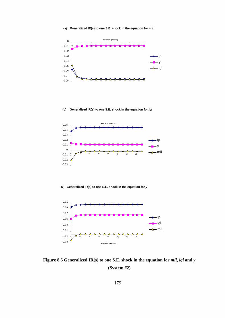
179

(a) Generalized IR(s) to one S.E. shock in the equation for mii

(b) Generalized IR(s) to one S.E. shock in the equation for igi

(c) Generalized IR(s) to one S.E. shock in the equation for y

Figure 8.5 Generalized IR(s) to one S.E. shock in the equation for mii, igi and y

(System #2)

-0.08

-0.07

-0.06

-0.05

-0.04

-0.03

-0.02

-0.01

0

0 2 4 6 8 10 12 14

Horizon (Years)

ipyigi

-0.03

-0.02

-0.01

0

0.01

0.02

0.03

0.04

0.05

0 2 4 6 8 10 12 14

Horizon (Years)

ipymii

-0.03

-0.01

0.01

0.03

0.05

0.07

0.09

0.11

0 2 4 6 8 10 12 14

Horizon (Years)

ipigimii

Moreover, given the evidence on the short and medium-term complemen-

tarity between public and private investment, a rise in public investment in-

duces a further increase in national income. A rise in national income will, in

turn, increase the revenues of government, such as tax and seigniorage revenue,

and help to reduce the Þscal deÞcit and inßation over some period, but with

diminishing effects.

Finally, we examine the dynamic effects of a rise in (a positive unit shock

to) output on all the other variables. As panel (c) of Figure 8.4 reveals, the

short and the medium-run responses of private and public investments to a

rise in output is positive as expected. As panel (c) of Figure 8.4 makes clear,

the impact effects of a rise in output on both private and public investment

are only slightly different than medium-term effects. The short-run responses

of macroeconomic instability is negative (e.g. due to the positive effect of a

rise in output on revenues of government and, hence, on budget deÞcit and

inßation); however over the medium term this response approaches towards

zero.26

Impulse Response Analysis for System #2

Figure 8.5 present the generalized IRs for the System #2. Comparing Fig-

ure 8.5 with 8.4 reveals that the generalized IRs of the System #2 is quite

similar to that of System #1 hence can be interpreted similarly. However,

there is only one considerable difference. In the System #2, infrastructural

public investment is more seriously affected from a rise in macroeconomic in-

stability compared to total public investment in the System #1. This is consis-

tent with the observation that Turkey failed to make necessary infrastructural

investment due to the constraining effects of macroeconomic instability and

associated Þscal problems on the incumbent governments budgets during the

late 1990s, and hence experienced infrastructural bottlenecks, such as energy

26The dynamic effects of private investment shock are similar to public investment shockon all the other variables (simply replace ip with ig in panel (b) of Figure 8.4); therefore, itis not separately explained.

180

bottlenecks, during the late 1990s and the early 2000s.

8.4 Conclusion and Policy Implications

This chapter investigated the empirical relationships between macroeconomic

instability, public and private capital accumulation and growth in Turkey over

the period 1963-1999. The main conclusion is that the chronic macroeconomic

instability of the Turkish economy has seriously affected capital formation and

growth. Even though cointegration analyses presented some evidence on the

crowding-out effect of total public investment on private investment, there was

no signiÞcant effect of infrastructural public investment on private investment

in the long-run. However, impulse response analyses suggested a complemen-

tarity between private and public investment (and with its infrastructural com-

ponents) over the short and medium-run. All these results (plus the descriptive

evidence provided in Chapter 7) imply that the chronic macroeconomic insta-

bility seems to become a serious impediment to the public investment, and

has shattered, or even reversed, the long-run complementarity. This result

may also shed some light on the ambiguity concerning the empirical evidence

on complementarity (crowding-in) effect for the Turkish economy. Moreover,

given the evidence on the short and medium-term complementarity between

public and private investment, these results also imply that macroeconomic

instability has been very costly in terms of private capital accumulation and

economic growth during the chronic instability episode of Turkey.

The policy implications are straightforward when these results are con-

sidered. Generally speaking, over the last twenty-Þve years, governments in

Turkey either delayed or did not continue with the stabilization programs. The

barriers to stabilization, such as political instability and polarization, are well-

documented in Veiga (2000) and Drazen (2000) among others. Nevertheless,

as this study shows, macroeconomic instability has an adverse impact on cap-

181

ital accumulation and economic growth in Turkey. Therefore, the government

should continue the current stabilization program to restore macroeconomic

stability, as soon as possible. This is the Þrst policy implication. The second

policy implication is that policy makers have to be careful in their decisions

concerning the components of public spending that would bear the burden of

Þscal adjustment in the process of the restoration of macroeconomic stabil-

ity. If government reduces public capital spending (especially, infrastructural

spending) instead of current and popular spending; then, this would harm capi-

tal accumulation, economic growth and development.27 Furthermore, as noted

in Section 2.5, Þscal adjustments entailing largely current or social transfer

expenditure cuts can be expansionary.

In sum, Turkish experience has shown that macroeconomic instability not

only deters economic growth but it may also reverse the complementarity be-

tween public and private investment in the long-run.

27See Sections 2.2 and 6.2 for the crucial importance and the multi-dimensional roles ofinfrastructure in economic growth and development.

182

CHAPTER 9

CONCLUSIONS

This conclusion chapter summarizes the main results of both Part I and II

and, then, provides the policy implications for Turkey.

Part I has developed a simple macroeconomic framework to provide insights

into the understanding of several politico-economic and institutional issues re-

lated to Þscal policy making in general and public spending and borrowing

in particular. They include the role of political instability on public spend-

ing and borrowing decisions and macroeconomic performance; composition of

Þscal adjustments; the role of corruption on quality of public investment and

macroeconomic performance; and capital borrowing rule.

The main features of the models developed in Part I are that two types of

public spending (productive vs. non-productive spending) are distinguished

and policy makers choice for one type of public spending over the other is

taken to be determined by a set of political economy factors. This framework

is also extended later by incorporating the public borrowing decisions.

The main results of Part I can be summarized as follows: It is shown that

the two types of public spending have asymmetric effects on future macroe-

conomic performance. While productive public spending has favorable effects

183

on output and inßation in the next period, popular (or unproductive) public

spending has unfavorable effects. The interesting result is that the beneÞcial

effects of productive spending are not only limited to output and inßation but

also includes future popular spending. Therefore, raising popular spending at

the expense of productive spending is associated with a less favorable macroe-

conomic performance in terms of future output and inßation as well as future

popular spending.

Part I has also attempted to provide some political economy explanations

to myopic and populist policies and resultant undesirable macroeconomic out-

comes. In other words, Part I has investigated the role of socio-political insta-

bility on macroeconomic policy making and macroeconomic instability. It is

shown that a high level of political instability may lead to myopic policies (via

electoral uncertainty) in the form of low level of public investment, and exces-

sive debt accumulation or inefficient budget deÞcits. Similarly, it is shown that

in countries with greater income inequality, social and ethnic fractionalization

and the resulting political instability, governments are more likely to opt for

popularity-enhancing (non-productive) spending at the expense of cutting back

on productivity-enhancing spending such as public investment. Myopic and

populist policies, in turn, lead to higher inßation, and lower output and public

spending. Thus, such policies result in a worse macroeconomic performance,

in the following period. These results are in line with the existing literature

but the distinguishing feature of the framework of Part I is that it focuses on

the productivity enhancing role of public investment and also links the overall

macroeconomic performance to decisions regarding the composition of public

spending.

This macroeconomic framework also enabled us to analyze the impact of

productivity enhancing public investment on macroeconomic performance both

in a centralized and a decentralized policy making structure. The main Þnd-

ings of Part I hold under both centralized and decentralized policy making

184

frameworks. However, an interesting result is that the delegation of mone-

tary policy making to an independent central bank may not necessarily result

in better macroeconomic performance (e.g. lower level of inßation), given

the importance of favorable effects of productive public spending on future

macroeconomic performance and the role of seigniorage as a source of Þnance,

especially in developing countries.

Part I has also provided a political economy explanation for the observed

expansionary (Non-Keynesian) output effects of some types of Þscal consolida-

tions. Previous studies on expansionary Þscal contractions suggested several

channels for those Non-Keynesian effects, such as the favorable wealth and

expectations effects of a cut in public consumption on private consumption.

In contrast, this study suggests an alternative channel for Non-Keynesian ef-

fects of Þscal adjustments based on the productivity enhancing role of pro-

ductive public spending. Within the context of the framework of Part I, it is

shown that in the event of an incumbent government reducing popular pub-

lic spending rather than public investment, which is a politically risky option,

Non-Keynesian effects are achieved. However, if the incumbent chooses a polit-

ically less risky option and reduces public investment instead of popular public

spending, the conventional or Keynesian effects are achieved.

Part I also highlighted the importance of the qualitative aspects of Þscal

policy for macroeconomic performance. More speciÞcally, this part developed

a simple framework to provide insights into the understanding of recently ob-

served empirical regularities on the detrimental effects of corruption on public

investment and output performance. It is shown that the size of the favorable

effect of public investment on macroeconomic performance depends positively

on its quality and hence is inversely related to the level of corruption in the

economy.

Additionally, this part has investigated the consequences of productive pub-

lic spending Þnanced by public borrowing on macroeconomic performance. It

185

is shown that productive spending, e.g. public investment, Þnanced by public

borrowing may or may not have favorable effects on the next periods macroe-

conomic performance. An interesting as well as original result is that the net

effect of productive public spending on the next periods macroeconomic per-

formance depends on the beneÞts of productive public spending relative to

the costs of public borrowing. In effect, there are three cases. If the beneÞts

of productive public spending exceeds (falls short of) the costs of borrowing

in the next period, then a net effect of current spending on productive pub-

lic expenditures on the next periods macroeconomic performance is favorable

(unfavorable). Additionally, if the beneÞts of productive public spending are

exactly equal to the costs of borrowing in the next period, then productive

public spending committed in the current period has no effect on macroeco-

nomic performance in the next period. In other words, in this case, the net

beneÞt of productive public spending is zero.

Likewise, the implications of a capital borrowing rule on public spending

decisions and macroeconomic performance have been investigated. It is shown

that even under a capital borrowing rule, higher public investment may yield

unfavorable effects on macroeconomic performance in the next period if the

beneÞts of productive public spending are low, e.g. due to low quality, vis-a-

vis its costs. It is also shown that while the capital borrowing rule prevents

strategic debt accumulation, it does not necessarily prevent the strategic use

of public investment.

Finally, it should be noted that the framework of Part I can be extended in

several ways. For example, an interesting extension of this framework would

be to endogenize the probability of electoral success by linking the electoral

outcome in the second period to the macroeconomic performance in the Þrst

period. In this way, the beneÞts of popular or non-productive public spending

may be even greater in the Þrst (pre-election) period since in this framework

while the beneÞts of popular public spending are enjoyed contemporaneously,

186

the beneÞts of public investment are enjoyed with a lag.

Part II has investigated the role of macroeconomic instability on public

and private capital accumulation and growth in Turkey over the 1963-1999

period. More speciÞcally, Part II has extended recent empirical studies in

the literature on the role of public investment in capital accumulation and

economic growth, by including macroeconomic instability and considering the

Turkish experience. To this end, after providing a detailed descriptive analysis,

Part II has investigated the empirical relationships between macroeconomic

instability, public investment, private investment and output in Turkey for the

1963-1999 period by using modern time series techniques, such as cointegration

and generalized impulse response analyses.

The main results of Part II can be summarized as follows: Both the de-

scriptive and econometric evidence suggests that the chronic and increasing

macroeconomic instability of the Turkish economy has seriously affected its

capital formation and growth. Furthermore, the Turkish experience indicates

that chronic macroeconomic instability seems to be a serious impediment to

public investment, especially to its infrastructural component, and shatters, or

even reverses, the complementarity between public and private investment in

the long-run. These results may also shed some light on the ambiguity concern-

ing the empirical evidence on the complementarity between public and private

investment for the Turkish economy. Given the evidence on the short and

medium-run complementarity, these results imply that macroeconomic insta-

bility has been very costly in terms of private capital accumulation. Thus, the

main conclusion from Part II is that macroeconomic instability not only deters

economic growth but it may also reverse the complementarity between public

and private investment in the long-run. However, in order to shed more light

on this result, this study can be further extended to other developing countries

suffering from chronic instability like Turkey and this is left for future research.

Nevertheless, the following Þnal remarks can be made from the Turkish

187

experience. Chronic macroeconomic instability and recurrent crises have been

very costly for both the Turkish economy and the Turkish politics, in the sense

that Turkey has not realized its full economic potential and Turkish citizens

have not reaped the fruits of the resultant economic prosperity. Furthermore,

as it is evident from the experiences of the recent years, macroeconomic in-

stability aggravated Þscal stringency (mainly due to the heavy debt burden)

which in turn prevented the government from engaging in productive public

spending, such as spending on basic infrastructure, education and health that

are believed to be crucial for long-term growth and development.

Finally, the policy implications for Turkey can be summarized as follows:

First, the implementation of the current stabilization program should be con-

tinued to restore macroeconomic stability, which is a pre-condition for sustain-

able economic growth. Second, the policy makers should be more sensitive in

their decisions regarding the components of public spending that would bear

the burden of Þscal adjustment in the process of the restoration of macroe-

conomic stability. But along with the stabilization efforts, the current gov-

ernment should also raise the quality of public investment, for example, by

taking necessary measures to alleviate (or eliminate) the detrimental effects of

corruption and favoritism on the productivity of public investment.

188

APPENDICES

APPENDIX A

DERIVATION OF OUTPUT SUPPLY FUNCTION

Output is given by the following production function:

Yt = Nγt , (1)

where Yt and Nt represent output and labor in period t, and 0 < γ < 1.

Distortionary taxes, which are the only form of taxes available to the govern-

ment, are levied on output at the rate τ t. A representative competitive Þrms

problem is to maximize proÞts PtNγt (1− τ t)−WtNt, where Pt and Wt repre-

sent price level and the wage rate in period t. A representative competitive

Þrm chooses labor Nt to maximize proÞts by taking Pt and Wt as given. The

resulting (log) output supply function is yt = α(pt−wt − τ t) + z, where lowercase letters represent logs, e.g. yt = ln(Yt), α = γ/(1 − γ), z = αln(γ) and

ln(1 − τ) is approximated with −τ . Normalizing output by subtracting theconstant term z = αln(γ) from yt yield the normalized output supply func-

tion xt = α(pt − wt − τ t). Utilizing wt = pet , where superscripts e denote

expectation,1 yield the output supply function in Equation (3.1).

1This condition implies that workers or centralized trade union set the nominal (log)wage to expected (log) price level. However, workers, via trade union, may set the nominal(log) wage w to achieve (log) target real wage v, i.e. wt = pet + v (see, for instance, Alesinaand Tabellini, 1987: 621-2, for more detail). In the above case, for the sake of simplicity, vis normalized to zero. This assumption does not affect qualitative nature of the results andit is also made by Beetsma and Bovenberg (1997a, 1997b,1999) among others with similarclaim.

189

APPENDIX B

DERIVATION OF THE BUDGET CONSTRAINT

Equation (3.3) is derived as follows (see Alesina and Tabellini, 1987; and

Beetsma and Bovenberg, 1999, for more detail). First of all, the government

budget constraint is stated in nominal terms:

PtGt = τ tPtXt +∆Mt (2)

where Gt represents real government spending, Mt represents money sup-

ply, and other terms are as deÞned earlier (see Appendix A).

Now, dividing both sides of the above equation with nominal income PtXt

gives the following

gt = τ t +∆Mt

PtXt. (3)

Money demand equation is based on a simple quantity theory framework,

Mt = kPt eX, (4)

where eX is some measure of (real) output , which is independent of tax

rate τ t, and k ≥ 0. Thus, total seigniorage revenue ∆Mt

Ptis given by

190

∆Mt

Pt= πtk eX (5)

where πt = ∆PtPt.

By utilizing the above equation and approximating eX with Xt, as with the

most of the literature noted in the text, Equation (3) can be re-expressed as

follows

gt = τ t + kπt. (6)

Similarly, by following most of the literature (including Alesina and Tabellini,

1987; Jensen, 1994; Debelle and Fischer, 1994; and Ozkan, 1998, 2000), and

assuming k = 1 for simplicity, Equation (3.3) is obtained.

191

APPENDIX C

DERIVATION OF THE POLICY OUTCOMES OF THE

BENCHMARK MODEL

In this set-up, the central policy maker minimizes the Loss function subject

to the constraints; namely, budget constraint and output supply function.2

Therefore, by substituting output supply function into the loss function, the

Lagrangean of the policy maker can be written as follows

$ =1

2[δ1π

2t + (α(πt − πet − τ t)− xt)2 + δ2(gt − gt)2] + λ(gt − τ t − πt) (7)

where λ is the Lagrange multiplier related to the budget constraint of the

central policy maker.

The Þrst-order conditions (FOCs)3 for π, τ and g can be written as follows,

respectively:

δ1πt + α(α(πt − πet − τ t)− xt) = λ (8)

−α(α(πt − πet − τ t)− xt) = λ (9)

2The timing of events is important. In this set-up (and also in the dynamic set-up),central policy maker acts after the nominal wages are set, as is standard in policy gamesliterature.

3FOCs are both necessary and sufficient for the optimum due to the quadratic-linearset-up.

192

δ2(gt − gt) = λ (10)

By eliminating λ from the above system and imposing rational expectations

condition (i.e. πet = πt), the following is obtained

πt =2α

δ1(ατ t + xt) (11)

(gt − gt) =α

δ2(ατ t + xt) (12)

Combining the above two equations with the budget constraint (and out-

put supply function) gives us the equilibrium policies appearing in the text

[Equations (3.4)-(3.7)].

193

APPENDIX D

DERIVATION OF AUGMENTED OUTPUT SUPPLY

FUNCTION

Output is given by the following production function:

Yt = AtNγt , (13)

where At represents the level of productivity in period t, 0 < γ < 1 and

other variables are as deÞned in Appendix A. Again, distortionary taxes are

levied on output at the rate τ t. In this case, a representative competitive Þrms

problem is to maximize proÞts

Pt(1− τ t)AtNγt −WtNt. (14)

A representative competitive Þrm chooses labor Nt to maximize proÞts by

taking Pt, Wt and At as given. The resulting (log) output supply function is

yt = α(pt +1

γat − wt − τ t) + z, (15)

where all variables are as deÞned in Appendix A.

As mentioned in the text, in this set-up it is assumed that the previous

periods productive public spending (gp) enhances the current periods pro-

ductivity level. More formally, (log) productivity is modelled as follows:

194

at = a0 + ζgpt−1, (16)

where ζ is productivity coefficient measuring extent by which one periods

productive public spending improves the (log) productivity in the following

period and ζ > 0.

Substituting Equation (16) into (15); then, normalizing output by sub-

tracting the constant term z0 = z + αa0/γ for simplicity and Þnally utilizing

wt = pet as in Appendix A, yields the augmented (normalized) output supply

function in Equation (3.8).

195

APPENDIX E

DERIVATION OF THE EQUILIBRIUM POLICY OUTCOMES

OF THE BASIC DYNAMIC MODEL

As mentioned before, in this two-period set-up, equilibrium outcomes are

derived by backwards induction. Therefore, for a given gp1, policy outcomes

and welfare losses for t = 2 are derived Þrst. Then, equilibrium outcomes for

t = 1 are derived.

Solution in t = 2

Solution in the Þnal period (t = 2) is similar to the benchmark case. For a

given gp1 , the central policy maker minimizes its in-period losses subject to the

budget constraint and output supply function, and with respect to π2, τ2 and

gnp2 (recall that gp is not among the choice variables in t = 2).

Therefore, by substituting output supply function into the loss function

(in t = 2), the Þnal-period Lagrangean of the policy maker can be written as

follows

$2 =1

2[δ1π

22+(α(π2+ρg

p1−πe2−τ2)−x2)2+δ2(gnp2 −gnp2 )2]+λ2(gnp2 −τ 2−π2)

(17)

where λ2 is the Lagrange multiplier related to the budget constraint of the

central policy maker in the Þnal period.

196

The FOCs for π2, τ2 and gnp2 can be written as follows, respectively:

δ1π2 + α(α(π2 + ρgp1 − πe2 − τ 2)− x2) = λ2 (18)

−α(α(π2 + ρgp1 − πe2 − τ2)− x2) = λ2 (19)

δ2(gnp2 − gnp2 ) = λ2 (20)

By eliminating λ2 from the above system and imposing RE condition (i.e.

πe2 = π2), the following is obtained

π2 =2α

δ1(ατ 2 + x2 − αρgp1) (21)

(g2 − g2) =α

δ2(ατ 2 + x2 − αρgp1) (22)

Combining the above two equations with budget constraint and output

supply function the optimal policy outcomes for the second period is found,

for a given gp1 [See Table 3.2]. Substituting these optimal policy outcomes

into the Loss function, a Þnal period loss of (δ2/2)D(x2/α + gnp2 − ρgp1)2 is

obtained, where D = (2δ2/δ1)Ψ2+Ψ. Note that this is smaller than the losses

achieved in the benchmark case with no productivity effect, which is given by

(δ2/2)D(x2/α+ g2)2 for t = 2.

Solution in t = 1

In the Þrst period (t = 1), the central policy maker minimizes its intertem-

poral loss function with respect to π1, τ1, gnp1 and gp1. Formally, by substituting

197

equilibrium values from t = 2 and output supply function (in t = 1)4 into the

intertemporal loss function, the Þrst-period Lagrangean of the policy maker

can be written as follows

$1 =1

2[δ1π

21 + (α(π1 − πe1 − τ 1)− x1)2 + δ2(gnp1 − gnp1 )2 + δ3(gp1 − gp1)2]

+βG(δ2/2)D(x2/α+ gnp2 − ρgp1)2 + λ1(gnp1 + gp1 − τ1 − π1) (23)


central policy maker in the Þrst period.

The FOCs for π1, τ1, gnp1 and gp1 can be written as follows, respectively:

δ1π1 + α(α(π1 − πe1 − τ 1)− x1) = λ1 (24)

−α(α(π1 − πe1 − τ1)− x1) = λ1 (25)

δ2(gnp1 − gnp1 ) = λ1 (26)

δ3(gp1 − gp1) + ρβGδ2D(x2/α+ gnp2 − ρgp1) = λ1 (27)

After eliminating λ1 from the above system and imposing rational expec-

tations condition (i.e. πe1 = π1), the relevant equations are combined with

budget constraint and output supply function to Þnd equilibrium values for

the Þrst period appearing in Table 3.2.

4Note that in our two-period set-up, gp0 is not included in the output supply function int = 1: α(π1 − πe1 − τ1). Nevertheless, our main results in this chapter would not change ifwe consider the following supply function in t = 1: α(π1 + ρg

p0 − πe1 − τ1).

198

APPENDIX F

DERIVATION OF THE POLICY OUTCOMES OF THE

DECENTRALIZED BENCHMARK MODEL

In this decentralized policy making framework, Þscal authority (govern-

ment) and independent central bank (CB) plays a one-shot Nash game. There-

fore, after the nominal wages are set, both Þscal and monetary authority act

simultaneously and non-cooperatively to choose their respective instruments.

Formally speaking, central bank optimally selects its policy by minimiz-

ing its Loss function [Equation (3.11)] subject to the output supply function

[Equation (3.1)] and with respect to π, taking the governments action and

expectations as given. Hence, CB minimizes the following expression with

respect to π

1

2[µ1π

2t + (α(πt − πet − τ t)− xt)2 + µ2(gt − gt)2] (28)

The Þrst-order condition for π yields the following equation, which is CBs

reaction function,

πt =α

µ1 + α2[α(πet + τ t) + xt] (29)

Similarly, the Þscal authority minimizes the Loss function [Equation (3.2)],

by taking central banks action and expectations as given, subject to the con-

straints; namely, budget constraint and output supply function, and with re-

199

spect to τ and g. Therefore, by substituting output supply function into the

loss function, the Lagrangean of the policy maker can be written as follows

$ =1

2[δ1π

2t + (α(πt − πet − τ t)− xt)2 + δ2(gt − gt)2] + λ(gt − τ t − πt) (30)

where λ is the Lagrange multiplier related to the budget constraint of the

Þscal authority.

The FOCs for τ and g can be written as follows, respectively:

−α(α(πt − πet − τ t)− xt) = λ (31)

δ2(gt − gt) = λ (32)

By eliminating λ from the above two-equation system, the following equa-

tion is obtained

(gt − gt) = −α

δ2[α(πt − πet − τ t)− xt] (33)

Combining the above equation with the budget constraint, the govern-

ments reaction function is obtained,

τ t =1

δ2 + α2[(α2 − δ2)πt − α2πet − αxt + δ2gt] (34)

After imposing the rational expectations condition (i.e. πet = πt) on the

above two reaction functions, equilibrium values of π and τ are obtained by

200

substituting relevant reaction function into each other. Similarly, the equi-

librium values of g and x are arrived at by using the budget constraint and

output supply function. These results appear in Table 3.6.

201

APPENDIX G

DERIVATION OF THE EQUILIBRIUM POLICY

OUTCOMES OF THE BASIC DYNAMIC MODEL

UNDER ELECTORAL UNCERTAINTY

In the two-period set-up, equilibrium outcomes are derived by backwards

induction as in Appendix E. Therefore, for a given gp1, policy outcomes and

welfare losses for t = 2 are derived Þrst. Then, equilibrium outcomes for t = 1

are derived.

Solution in t = 2

As elections are held at the end of t = 1 all policy decisions in t = 2 are

taken as in Appendix E ( i.e. in the absence of electoral uncertainty) and the

optimal policy outcomes for the second period, for a given gp1 , are the same as

in Table 3.2 of the previous chapter. (see Appendix E and Table 3.2 of the

previous chapter for more detail)

Solution in t = 1


poral loss function with respect to π1, τ1, gnp1 and gp1. Formally, by substituting

equilibrium values from t = 2 and output supply function (in t = 1) into the



$1 =1

2[δ1π


202

+pβG(δ2/2)D(x2/α+ gnp2 − ρgp1)2 + λ1(gnp1 + gp1 − τ1 − π1) (35)

where λ1 is Lagrange multiplier related to the budget constraint of the


The FOCs for π1, τ1, gnp1 and gp1 can be written as follows, respectively:

δ1π1 + α(α(π1 − πe1 − τ 1)− x1) = λ1 (36)

−α(α(π1 − πe1 − τ1)− x1) = λ1 (37)

δ2(gnp1 − gnp1 ) = λ1 (38)

δ3(gp1 − gp1) + ρpβGδ2D(x2/α+ gnp2 − ρgp1) = λ1 (39)



budget constraint and output supply function to Þnd the equilibrium values

for the Þrst period appearing in Table G.1.

203

Table G.1. Equilibrium Macroeconomic Outcome Under Electoral

Uncertainty in t = 1 and t = 2

gp,E1 = Θ∗[ δ3δ2Ψgp1 − gnp1 + Γ∗gnp2 − 1

αx1 +

Γ∗αx2]

gnp,E1 = −δ3δ2Θ∗gp1 + (1−Φ∗) gnp1 − Λ∗Θ∗gnp2 − 1

αΦ∗x1 − Λ∗Θ∗ 1αx2

πE1 =2δ2δ1[ δ3δ2Θ∗gp1 + Φ

∗gnp1 + Λ∗Θ∗gnp2 + Φ

∗ 1αx1 + Λ

∗Θ∗ 1αx2]

xE1 = −δ2α[ δ3δ2Θ∗gp1 + Φ

∗gnp1 + Λ∗Θ∗gnp2 + Λ

∗Θ∗ 1αx2] +Υ

∗x1

τE1= δ2

α2[ δ3δ2Θ∗gp1 + Φ

∗gnp1 + Λ∗Θ∗gnp2 + Λ

∗Θ∗ 1αx2]−Υ∗ 1αx1

gnp2 = Ψ(φ+ ρΓ∗Θ∗)gnp2 − 1αΨΞ∗x2 + ρΨ[ δ3δ2ΨΘ

∗gp1 −Θ∗gnp1 −Θ∗ 1αx1]πE2 =

2δ2δ1ΨΞ∗[ 1

αx2 + g

np2 ]− ρ2δ2δ1 Ψ[ δ3δ2ΨΘ∗g

p1 −Θ∗gnp1 −Θ∗ 1αx1]

xE2 = (z+ δ2α2ΨρΓ∗Θ∗)x2 − δ2

αΨΞ∗gnp2 +

δ2αΨρ[ δ3

δ2ΨΘ∗gp1 −Θ∗gnp1 −Θ∗ 1αx1]

τE2 = (δ2α2Ψ+ ρΓ∗Θ∗z)gnp2 −zΞ∗ 1

αx2 + ρz[ δ3δ2ΨΘ

∗gp1 −Θ∗gnp1 −Θ∗ 1αx1]


δ1,Ψ = 1

(1+φ),z = (1− δ2

α2Ψ) > 0, D = 2δ2

δ1Ψ2 +Ψ,β∗G =

pβG,Λ∗ = ρβ∗GD, Γ

∗ = Λ∗Ψ=

ρβ∗GΨD,Θ∗ = 1

(1+Ω∗) ,Ω∗ =

(δ3δ2+ρΛ∗)Ψ

, 0 < Φ∗ =ΨΩ∗(1+Ω∗) < 1,Ξ

∗ = 1− ρΘ∗Γ∗ > 0,Υ∗ = ¡1− δ2

α2Φ∗

¢> 0.

204

APPENDIX H

DERIVATION OF THE NEW BUDGET CONSTRAINT

Equation (5.3) can derived by following the similar steps as in Appendix

B (See, Beetsma and Bovenberg (1999) for more detail). First of all, the new

government budget constraint in nominal terms is stated:

PtGnpt + (1 + rt−1)PtDt−1 = τ tPtXt +∆Mt + PtDt (40)

where Gnpt represents the real (non-productive) government spending, Dt−1

denotes the real value of single-period indexed public debt issued in period t−1(i.e. public debt issued in period t− 1 matures in one period and paid back atthe end of period t), rt−1 represents the real interest rate in period t − 1 andDt represents the real value of new debt issue in period t, and all the other

variables are as deÞned before (see Appendices A and B).

Now, dividing both sides of the above equation with nominal income PtXt

gives the following

gnpt + (1 + rt−1)dt−1 = τ t + dt +∆Mt

PtXt(41)

Assuming that money demand equation is based on a simple quantity the-

ory framework (i.e. Mt = kPt eX) as in Appendix B and following the rest ofthe steps therein leads to Equation (5.3).

205

APPENDIX I

DERIVATION OF THE EQUILIBRIUM POLICY

OUTCOMES OF AN EXTENDED BENCHMARK

MODEL WITH DEBT DYNAMICS

In this two-period set-up, equilibrium outcomes are derived by backwards

induction as in Appendix E.

Solution in t = 2

Solution in t = 2 is similar to the basic dynamic model. That is, d2 is

not among the choice variables in t = 2; therefore, for a given d1, the central

policy maker minimizes its in-period losses subject to the budget constraint

and output supply function, and with respect to π2, τ 2 and gnp2 . Thus, by

substituting output supply function into the loss function, the Þnal-period

Lagrangean of the policy maker can be written as follows

$2 =1

2[δ1π

22 + (α(π2 − πe2 − τ2)− x2)2 + δ2(gnp2 − gnp2 )2]

+λ2(gnp2 + (1 + r1)d1 − τ2 − π2) (42)




206

δ1π2 + α(α(π2 − πe2 − τ 2)− x2) = λ2 (43)

−α(α(π2 − πe2 − τ2)− x2) = λ2 (44)

δ2(gnp2 − gnp2 ) = λ2 (45)

By eliminating λ2 from the above system and imposing rational expecta-

tions condition (i.e. πe2 = π2), the following is obtain

π2 =2α

δ1(ατ 2 + x2) (46)

(g2 − g2) =α

δ2(ατ 2 + x2) (47)

Combining the above two equations with budget constraint and output

supply function yields the optimal policy outcomes for the second period, for

a given d1 (see Table 5.1). By substituting these optimal policy outcomes into

the Loss function, a Þnal period loss of (δ2/2)D(x2/α + gnp2 + (1 + r1)d1)

2 is

obtained, where D = (2δ2/δ1)Ψ2 +Ψ.

Solution in t = 1


poral loss function with respect to π1, τ1, gnp1 and d1. Formally, by substituting

equilibrium values from t = 2 and output supply function (in t = 1)5 into the



5Note that in this two-period set-up, d0 is not included in the budget constraint of thecentral policy maker in t = 1 (Recall that gp0 is not included in the supply function in thebasic dynamic model of Chapter 3). However, qualitative nature of our results would notchange.

207

$1 =1

2[δ1π

21 + (α(π1 − πe1 − τ 1)− x1)2 + δ2(gnp1 − gnp1 )2] + βG(δ2/2)D

(x2/α+ gnp2 + (1 + r1)d1)

2 + λ1(gnp1 − τ1 − π1 − d1) (48)



The FOCs for π1, τ1, gnp1 and d1 can be written as follows, respectively:

δ1π1 + α(α(π1 − πe1 − τ 1)− x1) = λ1 (49)

−α(α(π1 − πe1 − τ1)− x1) = λ1 (50)

δ2(gnp1 − gnp1 ) = λ1 (51)

(1 + r1)βGδ2D(x2/α+ gnp2 + (1 + r1)d1) = λ1 (52)





208

APPENDIX J

DERIVATION OF THE EQUILIBRIUM POLICY OUTCOMES

OF THE DOUBLE DYNAMICS MODEL

Equilibrium outcomes are derived by backwards induction as in Appendices

E and I.

Solution in t = 2

In t = 2, for a given values of d1 and gp1 , the central policy maker minimizes

its in-period losses subject to the budget constraint and output supply func-

tion, and with respect to π2, τ 2 and gnp2 (Recall that d1 and g

p1 are not among

the choice variables in t = 2). By substituting output supply function into the

loss function, the Þnal-period Lagrangean of the policy maker can be written

as follows

$2 =1

2[δ1π

22 + (α(π2 + ρg

p1 − πe2 − τ 2)− x2)2 + δ2(gnp2 − gnp2 )2]

+λ2(gnp2 + (1 + r1)d1 − τ2 − π2) (53)




209

δ1π2 + α(α(π2 + ρgp1 − πe2 − τ 2)− x2) = λ2 (54)

−α(α(π2 + ρgp1 − πe2 − τ2)− x2) = λ2 (55)

δ2(gnp2 − gnp2 ) = λ2 (56)

By following the same steps as in Appendices E and I, optimal policy

outcomes for the second period are attained, for a given levels of d1 and gp1

(see Table 5.5). By substituting these optimal policy outcomes into the Loss

function, a Þnal period loss of (δ2/2)D(x2/α + gnp2 + (1 + r1)d1 − ρgp1)2 is

obtained, where D = (2δ2/δ1)Ψ2 +Ψ.

Solution in t = 1

In t = 1, the central policy maker minimizes its intertemporal loss function

with respect to π1, τ 1, gnp1 , g

p1 and d1. Formally, by substituting equilibrium

values from t = 2 and output supply function (in t = 1)6 into the intertemporal

loss function, the Þrst-period Lagrangean of the policy maker can be written

as follows

$1 =1

2[δ1π


+βG(δ2/2)D(x2/α+ gnp2 + (1 + r1)d1 − ρgp1)2

+λ1(gnp1 + gp1 − τ1 − π1 − d1) (57)



6Note that, as before d0 and gp0 are not included in t = 1, which would not change

qualitative nature of the results.

210

The FOCs for π1, τ1, gnp1 , g

p1 and d1 can be written as follows, respectively:

δ1π1 + α(α(π1 − πe1 − τ 1)− x1) = λ1 (58)

−α(α(π1 − πe1 − τ1)− x1) = λ1 (59)

δ2(gnp1 − gnp1 ) = λ1 (60)

δ3(gp1 − gp1) + δ2ρβGD(x2/α+ gnp2 + (1 + r1)d1 − ρgp1) = λ1 (61)

δ2(1 + r1)βGD(x2/α+ gnp2 + (1 + r1)d1 − ρgp1) = λ1 (62)





211

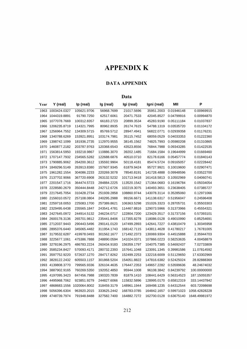
212

APPENDIX K

DATA APPENDIX

DataYear Y (real) Ip (real) Ig (real) Igi (real) Igni (real) MII P1963 1003424.0327 105621.9706 56968.7699 21017.5696 35951.2003 0.01946148 0.009699151964 1044319.8891 91790.7250 62517.6061 20471.7533 42045.8527 0.04799916 0.009948701965 1077078.7669 100312.8357 66183.2723 20899.3534 45283.9190 0.05111184 0.010378371966 1206235.8719 114321.7995 80962.8935 26174.7615 54788.1319 0.03535720 0.011041721967 1256964.7552 134309.5715 85769.5712 28947.4941 56822.0771 0.02939358 0.011762311968 1340788.6269 153921.8951 103174.7981 35115.7452 68059.0529 0.04033353 0.012223601969 1398742.1099 181936.2735 112970.9555 38145.1562 74825.7993 0.05980208 0.013108651970 1460877.2182 203787.9763 120368.6543 43523.8556 76844.7988 0.09343285 0.014225351971 1563814.5950 193218.9867 110886.3070 39202.1485 71684.1584 0.19644999 0.016694601972 1707147.7932 234565.5282 122688.6876 40510.0710 82178.6166 0.05457774 0.018401431973 1790885.9062 264200.3612 135592.9904 50118.4181 85474.5724 0.09165057 0.022284421974 1849296.5149 263913.8380 157607.9345 61879.9424 95727.9921 0.10019600 0.029074711975 1961282.1554 304086.2233 220269.3078 78540.8191 141728.4888 0.09948596 0.035227001976 2137702.9066 367720.6908 263132.5232 101713.9418 161418.5813 0.10502969 0.040607411977 2201547.1716 364474.5723 284884.2225 113520.1542 171364.0683 0.16196784 0.050340541978 2228580.2679 350444.8448 242712.6726 102219.3075 140493.3651 0.23638405 0.073857271979 2217645.7054 310428.2734 251939.2858 108860.9744 143078.3114 0.35285060 0.129710661980 2156010.0572 257108.0804 240295.2988 99156.6671 141138.6317 0.51956047 0.245964081981 2259718.0053 225083.1700 257389.8621 106363.5298 151026.3323 0.28705731 0.355033031982 2329495.6438 235565.1847 243541.4781 114467.8816 129073.5966 0.31373966 0.455543211983 2427645.0972 244914.5132 246234.0717 122804.7200 123429.3517 0.31737156 0.573931011984 2600178.3136 265701.9812 235441.8406 117355.8278 118086.0128 0.49010990 0.852546911985 2712037.9443 290443.5496 290141.0120 147499.2893 142641.7227 0.43810479 1.303459581986 2895376.6440 345065.4482 311954.1743 168142.7115 143811.4628 0.41780217 1.767810051987 3179532.6287 419978.0493 301562.1677 171492.2373 130069.9304 0.44515888 2.359447031988 3225677.1061 475386.7888 248890.0594 141024.0371 107866.0223 0.58253635 4.004588791989 3278196.2975 486783.2224 260434.9183 156359.1797 104075.7385 0.54692437 7.027338091990 3585234.8427 570093.4171 280732.2393 157641.1048 123091.1345 0.39981586 11.078145921991 3597752.9220 572637.1270 284717.8262 152499.2253 132218.6009 0.51129650 17.633029691992 3828122.2432 605503.1157 301868.5204 154051.8822 147816.6382 0.52425024 28.828883691993 4139808.3770 799565.9336 326104.4635 176447.2353 149657.2282 0.53599636 48.246740321994 3887902.9165 760269.5350 192052.4850 95944.1008 96108.3842 0.84239792 100.000000001995 4197095.3423 847456.7988 190320.7839 81879.1410 108441.6429 0.56314523 187.150553571996 4495968.7062 923851.9279 244827.6066 115832.5896 128995.0170 0.65812319 333.144378421997 4868683.1556 1020064.8002 318459.3179 148961.1944 169498.1235 0.64312544 603.720986981998 5056396.6304 963920.2015 333625.2442 168783.0785 164842.1657 0.59971023 1058.428282281999 4748739.7974 791948.8488 327582.7400 164882.7272 162700.0128 0.63675140 1648.49981972

213

Data Definitions and Sources

Y (real) is the real GNP in 1994 prices (billion TL). Sources: Nominal GNP

series are obtained from SPO (1997: Table 1.1) and SPO (2001: Table II.3) for

1963-1996 and 1997-1999, respectively.

P is the real GNP Deflator (1994=100). Sources: SPO (1997: Table 1.1) and SPO

(2001: Tables II.3 and II.4) for 1963-1996 and 1997-1999, respectively.

Ip (real) is the real private fixed investments in 1994 prices (billion TL). Nominal

private fixed investment series are deflated by private fixed investment deflator

series. Sources: Nominal private fixed investment series are obtained from SPO

(1997: Table 2.4) and SPO (2001: Table IV.1) for 1963-1996 and 1997-1999,

respectively. Deflators are provided by the SPO.

Ig (real) is the real public fixed investments in 1994 prices (billion TL). Nominal

public fixed investment series are deflated by public fixed investment deflator

series. Sources: Nominal public fixed investment series are obtained from SPO

(1997: Table 2.4) and SPO (2001: Table IV.1) for 1963-1996 and 1997-1999,


Igi (real) is the real public fixed core infrastructural investments in 1994 prices

(billion TL). Nominal sectoral public fixed investment series are deflated by

relevant sectoral public fixed investment deflator series. In line with Ekinci (1990)

among others core infrastructural investment is defined as the total of the public

energy, transportation and communication sectors fixed investments. See World

Bank (1994: 2) for broad definition of infrastructure. [Note that non-core

infrastructural investment is defined as the total of the all sectors fixed

investments except public energy, transportation and communication sectors.

Thus, Igni (real), which denotes the real public fixed non-core infrastructural

214

investments in 1994 prices (billion TL), is calculated in similar way.] Sources:

Nominal sectoral public fixed investment series are obtained from SPO (1997:

Table 2.7) and SPO (2001: Table IV.1) for 1963-1996 and 1997-1999,


Macroeconomic instability index (MII) is calculated by using human

development index (HDI) methodology (UNDP, 1992) and it is based on four

macroeconomic instability indicators; namely, inflation rate, public deficit to GNP

ratio, external debt to GNP ratio and change in exchange rate (exchange rate

variability), identified by previous researchers (See Chapter 6). Note that the four

indicators are not in the same units and more importantly they have different

ranges, i.e. they have different minimums and maximums. Therefore, it seems not

sensible to sum their values or to take their simple average in order to obtain a

composite index. Fortunately, the HDI methodology circumvents these problems.

MII is, therefore, constructed in two steps utilizing this methodology. In the first

step, four sub-indices are constructed based on the general formula: It = (Xt -

XMin) / (XMax - XMin), where It refers to the index value of variable X, i.e.

macroeconomic instability indicator X, in year t, Xt refers to the actual value of

indicator X in year t, and XMin (XMax) refers to the minimum (maximum) value of

indicator X over the whole period under consideration (1963-99). Note that in line

with their construction, all sub-indices have common ranges, i.e. they are bounded

between 0 and 1. In the second and the final step, MII is constructed by taking

simple average of the four sub-indices obtained as above. Thus, MII is also

bounded between 0 and 1.

Note: (1) Inflation rate refers to the %-age change in GNP Deflator; (2) the

change in exchange rate is proxied by the %-age change in (year-average) US$

rate; (3) public deficit refers to the consolidated budget deficit; and (4) external

debt refers to medium and long term outstanding external public debt. Sources: (1)

Data sources for the GNP Deflator are given above. (2) Exchange rate (US$ rate)

data for 1963-1996 and 1997-1999, are obtained from SPO (1997: Table 3.14),

and SPO (2001: Table V.25), respectively. (3) Consolidated budget deficit to GNP

215

ratio data for 1963-1996 and 1997-1999, are obtained from SPO (1997: Tables 5.5

and 5.6), and SPO (2001:Table VI.2), respectively. While deficit is recorded as

(+), surplus is recorded as (-). Note that realized deficit (cash balance) figures are

used for the 1963-74 (1975-99) period (see SPO, 1997: Tables 5.5 and 5.6). There

is also difference in the revenue and the expenditure figures between the 1963-74

and 1975-99 periods due to accounting practice. That is, foreign and domestic

borrowing (repayment) are included in the revenues (expenditures) in 1963-74

period. (4) Data for medium and long term outstanding external public debt are

obtained from SIS (1994: Tables XVIII-10 and 11) and SPO (2001: Table V.24)

for 1964-1992 and 1993-1999, respectively. Medium and long term outstanding

external public debt figure for 1963 is not available but it is estimated backward

by using the growth rate of the total foreign debt from 1963 to 1964. The total

foreign debt data for 1963 and 1964 are obtained from SPO (1997: Table 3.12). It

should be also noted that during the late 1990s the Treasury revised the foreign

debt figures (see SPO, 2001: Table V.24). For the sake of consistency, figures for

1997-1999 period are obtained by extending the old series (1963-96) with the

growth rates obtained from the new series.

216

APPENDIX L

TURKISH SUMMARY

Türkiye ve birçok kalkõnmakta olan ülke (örneğin bazõ Latin Amerika ülkeleri)

uzun süreler boyunca popülist ve kõsa görüşlü (miyopik) politikalar izlediler. Bu

tür politikalarõn neticesinde, kronik makroekonomik istikrarsõzlõk (yüksek ve

oynak enflasyon oranõ; artan bütçe açõklarõ ve borç yükü; v.s.) ve bununla

bağlantõlõ olarak hayal kõrõklõğõ yaratan ekonomik performans (düşük ve oynak

sermaye oluşumu ve büyüme oranlarõ; tekrar eden krizler; v.s.) bu ülkelerin temel

makroekonomik sorunlarõ olmuştur.

Günümüzde birçok iktisatçõ sosyo-politik faktörlerin (örneğin gelir dağõlõmõndaki

adaletsizlik) kamu harcama ve borçlanma politikalarõ üzerinde önemli etkileri

olduğunu vurgulamaktadõr. Bazõ iktisatçõlar daha da ileri giderek, makroekonomik

istikrarsõzlõğa sebep olan popülist ve miyopik politikalarõn temelinde sosyo-politik

dengesizliklerin olduğunu söylemektedirler.

Bu doktora tezi iki kõsõmdan oluşmaktadõr. Tezin birinci kõsmõnda politik makro-

iktisat modelleri oluşturularak, bir takõm politik iktisat (ve kurumsal) faktörlerin

maliye politikalarõ ve makroekonomik performans üzerindeki rolü

incelenmektedir. Tezin ikinci kõsmõnda, Türkiye ekonomisindeki makroekonomik

istikrarsõzlõğõn sermaye birikimi ve ekonomik büyüme üzerindeki etkileri 1963-

1999 yõllarõ için araştõrõlmaktadõr.

217

BİRİNCİ KISIM: SİYASET, KAMU HARCAMALARI, BORÇLANMA VE

MAKROEKONOMİK PERFORMANS

Tezin bu kõsmõnda maliye politikalarõnõn oluşturulmasõ ile ilgili bazõ politik

makro-iktisat konularõnõn daha iyi anlaşõlmasõ için teorik bir çerçeve

oluşturulmaktadõr. Bu konular siyasi istikrarsõzlõğõn kamu harcama ve borçlanma

kararlarõ ve makroekonomik performans üzerindeki rolü; mali daralmalarõn

bileşimi; rüşvetin kamu yatõrõmlarõnõn kalitesi ve makroekonomik performans

üzerindeki rolü; ve sermaye borçlanma kuralõnõn (capital borrowing rule)

makroekonomik performans üzerindeki etkilerini içermektedir. Bu kõsõmda

oluşturulan modellerin en temel özelliği verimli (productive) ve verimsiz (non-

productive) kamu harcamalarõ arasõnda bir ayõrõmõn yapõlmasõdõr. Verimi artõran

ve dolayõsõyla üretim seviyesinde artõş yaratan bir kamu harcamasõ (örneğin kamu

altyapõ yatõrõmlarõ) verimli harcama olarak, tersi durumunda ise (örneğin genel

idare harcamalarõ) verimsiz harcama olarak sõnõflandõrõlmaktadõr. Bu modellerin

diğer bir temel özelliği ise hükümetin ya da politika yapõcõlarõn bazõ kamu

harcama türlerini diğer türlere tercih etmesinin bir takõm politik iktisat faktörler

tarafõndan belirlenmesidir.

Bu kõsõmdaki sonuçlarõ şu şekilde özetleyebiliriz. Farklõ tür kamu harcamalarõnõn

gelecekteki makroekonomik performans üzerinde asimetrik etkileri olduğu

gösterilmiştir. Verimli kamu harcamalarõndaki bir artõş bir sonraki dönemde

üretim seviyesi ve enflasyon oranõ üzerinde olumlu etki yaratõrken, popüler (veya

verimsiz) kamu harcamalarõndaki bir artõş bir sonraki dönemde aynõ

makroekonomik değişkenler üzerinde olumsuz bir etki yaratmaktadõr. İlginç olan

sonuç ise verimli kamu harcamalarõnõn olumlu etkilerinin sadece üretim ve

enflasyon ile kõsõtlõ olmamasõ ve gelecekteki popüler harcamalarõ da kapsamasõdõr.

Bu nedenle, popüler harcamalarõ verimli harcamalarõ azaltmak pahasõna artõrmak

gelecekte daha kötü bir makroekonomik performansa yol açabileceği, ve bunun

sadece gelecekteki üretim ve enflasyon açõsõndan değil aynõ zamanda gelecekteki

popüler harcamalar açõsõndan da kötü olabileceği gösterilmiştir.

218

Bu kõsõm, yukarõdaki sonuçlarla bağlantõlõ olarak, miyopik (myopic) ve popülist

(populist) politikalara ve bunlarõn makroekonomik performans üzerindeki

olumsuz etkilerine politik iktisat açõklamalarõ getirmeye çalõşmaktadõr. Diğer bir

deyişle, bu kõsõmda sosyo-politik istikrarsõzlõğõn ekonomik politikalarõn

oluşturulmasõndaki ve makroekonomik istikrarsõzlõk üzerindeki rolü incelenmiştir.

Örneğin yüksek düzeydeki siyasi istikrarsõzlõğõn (seçim belirsizliği vasõtasõyla),

kamu yatõrõmlarõnõn düşük seviyede gerçekleşmesine yol açarak, stratejik

davranõşa ve miyopik politikalara yol açabileceği gösterilmiştir. Yine benzeri

şekilde, yüksek düzeydeki siyasi istikrarsõzlõğõn aşõrõ (ve stratejik) borç birikimi

yaratarak miyopik politikalara yol açabileceği gösterilmiştir. Burada üzerinde

durulmasõ gereken husus, hem borçlanma hem de kamu yatõrõmlarõnõn bir zaman

unsuruna bağlõ olmalarõdõr. Başka bir deyişle, mevcut hükümetin borçlanma ve

kamu yatõrõmlarõ ile ilgili kararlarõ gelecekteki (fakat bugün itibariyle seçimlerden

dolayõ belirsiz olan) hükümetlerin kaynak ve harcamalarõnõ etkileyerek

gelecekteki ekonomik politikalarõ etkileyebilme özelliğine sahiptir. Ayrõca mevcut

hükümetin gelecek dönem için seçilme olasõlõğõnõn düşük olmasõ bu hükümeti

miyopik politikalar izlemeye teşvik etmektedir. Daha açõk bir ifadeyle anlatmak

gerekirse, mevcut hükümetin gelecek dönem için seçilme olasõlõğõnõn düşmesi

(örneğin politik istikrarsõzlõğõn artmasõndan dolayõ) bu hükümetin popüler

harcamalarõ verimli harcamalarõ azaltmak pahasõna artõrmasõna ve bu harcamalarõ

finanse etmek için aşõrõ borçlanmaya yönelmesine neden olabilmekte ve gelecekte

daha kötü bir makroekonomik performansa ve hatta istikrarsõzlõğa yol

açabilmektedir. Bu sonuçlar ilgili literatürdeki sonuçlar ile örtüşmektedir.

Aynõ şekilde, gelir dağõlõmõ adaletsizliğinin, sosyal ve etnik bölünmüşlüğün çok

yüksek düzeyde olduğu ülkelerde, ve bu sosyo-politik özellikler sonucunda siyasi

istikrarsõzlõğõnda yüksek düzeyde olduğu bu ülkelerin hükümetleri kamu yatõrõm

harcamalarõ gibi verimliliği artõrõcõ harcamalarõ azaltma pahasõna hükümetin

seçmenlerin gözünde popülerliğini artõran harcamalarõ artõrmasõ (örneğin kamu

çalõşanlarõna yapõlan ek maaş artõşlarõ ve sosyal harcamalardaki artõşlar) daha olasõ

olduğu birçok iktisatçõ tarafõndan bilinmektedir. Birinci kõsõmda oluşturulan teorik

çerçevede, hükümetlerin bu tür popülist davranõşlarõnõn, daha yüksek enflasyon

219

oranõna ve üretim ve kamu harcamalarõnõn azalmasõna yol açtõğõ gösterilmiştir.

Başka bir deyişle, bu tür politikalar bir sonraki dönemde daha kötü bir

makroekonomik performansa yol açmaktadõr. Bu sonuçlar mevcut literatürdeki

sonuçlar ile örtüşmektedir ancak birinci kõsõmda oluşturulan teorik çerçevenin

diğer çalõşmalardan ayõrt edici özelliği hem verimli kamu harcamalarõnõn

verimliliği artõrõcõ rolünün dikkate alõnmasõ hem de bu kurguda makroekonomik

performans ile hükümetin kamu harcamalarõ ile ilgili kararlarõnõn

ilişkilendirilmesidir.

Birinci kõsõmdaki teorik çerçeve bize aynõ zamanda iki tür kamu harcamasõnõn

makroekonomik performans üzerindeki etkilerini hem merkezi (mali ve para

otoritelerinin tek bir merkezi otoriteye ya da devlete bağlõ olduğu durumda) hem

de merkezi olmayan kurumsal yapõ (para otoritesinin, yani Merkez Bankasõnõn,

bağõmsõz olduğu durumda) çerçevesinde de incelemeye fõrsat tanõmaktadõr. Bu

kõsõmdaki temel sonuçlar (örneğin iki tür kamu harcamasõnõn asimetrik etkileri)

her iki kurumsal yapõda da nitel olarak da aynõdõr. Ancak, ilginç olan sonuç,

Merkez Bankasõnõn bağõmsõz olduğu durumda, özellikle gelişmekte olan

ülkelerdeki verimli kamu harcamalarõnõn gelecekteki makroekonomik performans

üzerindeki olumlu (ve göreceli olarak yüksek olmasõ beklenen) etkisi göz önünde

bulundurulduğunda, merkezi yapõya kõyasla daha iyi bir makroekonomik

performans (örneğin daha düşük bir enflasyon oranõna) sonucu

alõnamayabileceğidir.

Keynesyen veya geleneksel görüş mali daralmanõn ekonomi üzerinde daraltõcõ

etkisi olduğunu vurgulamaktadõr. Ancak, son yõllardaki araştõrmalar, özellikle

Danimarka ve İrlandanõn deneyimlerini inceleyenler, bazõ tür mali daralmalarõn

genişletici, yani Keynesyen olmayan (Non-Keynesian) etkileri ile ilgili ampirik

bulgular sunmaktadõr. Bu çalõşmalardan genişletici mali daralmalar diye

adlandõrõlan yeni bir literatür oluşmuştur. Bu literatürün ana mesajõ mali

daralmalarõn yapõsõnõn da önemli olduğudur. Örneğin hükümetin cari veya sosyal

transfer harcamalarõ yerine kamu yatõrõm harcamalarõnõ azaltmasõ durumunda

220

daraltõcõ bir etkinin gerçekleştiği, fakat bunun tersi olursa mali konsolidasyonlarõn

genişletici etkiye sahip olduğu vurgulanmaktadõr.

Genişletici mali daralmalar konusundaki mevcut çalõşmalar bu tür mali

daralmalarõn Keynesyen olmayan etkileri konusunda bazõ kanallar önermişlerdir.

Örneğin kamu tüketimindeki bir azalma olumlu servet etkisi ve bekleyiş etkisi

yaratarak özel tüketimi artõrabilmektedir. Buna karşõlõk, bu tezin birinci kõsmõnda,

verimli kamu harcamalarõnõn verimliliği artõrõcõ rolü dikkate alõnarak, Keynesyen

olmayan mali daralmalar için alternatif bir kanal önerilmektedir. Bu kõsõmda

oluşturulan kurguda, mevcut hükümetin siyasi olarak riskli olan seçeneği

uygulamasõ, yani kamu yatõrõmlarõndan ziyade popüler kamu harcamalarõnõ

düşürmesi durumunda, Keynesyen olmayan sonuçlar elde edilmektedir. Ancak,

mevcut hükümet siyasi olarak daha az riskli seçeneği seçerse, başka bir deyişle

hükümetin popüler harcamalar yerine verimli harcamalarõ azaltmasõ halinde

Keynesyen etkilere ulaşõlmaktadõr.

Birinci kõsõmda incelenen başka bir konu ise maliye politikalarõnõn nitel

unsurlarõnõn makroekonomik performans üzerindeki etkisi ve rolüdür. Özellikle,

son zamanlarda rüşvetin veya iltimasõn kamu yatõrõmlarõnõn kalitesi ve üretim

düzeyi üzerindeki olumsuz etkileri ile ilgili olarak elde edilen ampirik ilişkileri

anlamak için basit bir kurgu oluşturulmuştur. Bu çerçevede kamu yatõrõmlarõnõn

kalitesinin de kamu yatõrõmlarõnõn olumlu etkilerini pozitif yönde etkilediği

gösterilmiştir. Başka bir deyişle, rüşvet ve iltimasçõlõğõn kamu yatõrõmlarõnõn

kalitesini (verimliliğini) olumsuz yönde etkileyerek kamu yatõrõmlarõnõn

makroekonomik performans üzerindeki olumlu etkisini azaltmaktadõr.

Bazõ yazarlar stratejik borç birikimini (strategic debt accumulation) önlemek için

hükümetlerin belli kurallara bağlõ olarak borçlanmalarõnõ (yani bağlayõcõ borç

kurallarõ uygulanmasõnõ) ön plana çõkarmõşlardõr. Örneğin denk bütçe kuralõ özel

bir durumdur. Ancak, bu tür kurallarõn bazõ sakõncalarõ vardõr. En önemli sakõnca,

bağlayõcõ borç kurallarõnõn kamu yatõrõmlarõnõn azalmasõna yol açabileceğidir.

Örneğin Avrupa Parasal Birliğine üye birçok ülkenin İstikrar ve Büyüme Paktõ

221

tarafõndan empoze edilen kamu açõklarõ ile ilgili mali kurallara (denk bütçe

kuralõna yakõn) uymaya çalõşõrken kamu yatõrõmlarõnõ kõstõğõ geniş bir kitle

tarafõndan vurgulanmaktadõr. Aynõ şekilde, Avrupa Parasal Birliğinin

oluşturulmasõndan sonra Avrupadaki ekonomik büyümedeki yavaşlama birçok

yazarõn ilgisini bu tür kurallara çekmiştir.

Bunlarõn yanõ sõra, bazõ yazarlar sadece kamu yatõrõmlarõnõn finansmanõ için

hükümete borçlanma olanağõ tanõyan sermaye borçlanma kuralõnõn stratejik

(politik) davranõşlarõ engelleyebileceğini savunmaktadõrlar. Aynõ şekilde, böyle

bir kuralõn mali disiplin açõsõndan da önemli olduğu sõk sõk tartõşõlmaktadõr. Sonuç

olarak, bu kural sõkça kamu finansmanõnõn altõn kuralõ olarak da adlandõrõlmakta

ve birçok ABD eyaleti ve Hollanda belediyeleri tarafõndan uygulanmõştõr. Benzeri

altõn kural 1997den beri Yeni İşçi partisinin kamu yatõrõmlarõndaki düşüş

eğilimini tersine çevirme sözü ile iktidara geldiği Birleşik Krallõkta da

uygulanmaktadõr.

Kamu borçlanmalarõnõn ve sermaye boçlanma kuralõnõn kamu yatõrõmõ ve

makroekonomik performans üzerindeki rolünün anlaşõlmasõ kalkõnmakta olan

ülkeler açõsõndan da aşağõda bahsedeceğimiz nedenlerden dolayõ çok büyük bir

önem teşkil etmektedir. Öncelikle belirtmek gerekir ki, siyasi istikrarsõzlõk (ve

kutuplaşma) birçok gelişmekte olan ülkenin kamu borçlanma ve harcama kararlarõ

üzerinde önemli bir etkiye sahiptir. Buna ilaveten, kamu yatõrõmlarõnõn

verimliliğinin bu ülkelerde yüksek olmasõ beklenmektedir; böylece, verimsiz

(popüler) harcamalarõn kamu yatõrõmlarõnõ azaltma pahasõna tercih edildiği

politikalar bu ülkeler açõsõndan daha kötü bir etki yaratmaktadõr. Son olarak, bu

ülkelerde iç borçlanmanõn makroekonomik performans üzerinde, finansal

piyasalarõn az gelişmiş ya da sõğ olmalarõ ile bağlantõlõ olarak, ciddi etkileri vardõr.

Bu nedenlerden dolayõ, birinci kõsõmda son konu olarak kamu borçlanmasõnõn ve

sermaye borçlanma kuralõnõn kamu harcama politikalarõ, özellikle kamu

yarõrõmlarõ, ve makroekonomik performans üzerindeki etkileri incelenmektir.

222

Bu bağlamda, mevcut teorik çerçeve kamu borçlanma kararlarõ dahil edilerek

genişletilmiştir ve borçlanma ile finanse edilen verimli harcamalarõn, örneğin

kamu altyapõ yatõrõmlarõnõn, bir sonraki dönemdeki makroekonomik performans

üzerindeki net etkisinin olumlu veya olumsuz olabileceği gösterilmiştir. Başka bir

deyişle, borçlanma ile finanse edilen verimli harcamalarõn gelecek dönemdeki

makroekonomik performans üzerindeki net etkileri bu harcamalarõn olumlu

etkilerinin yanõ sõra borçlanmanõn maliyetinede bağlõdõr. Burada üç durum söz

konusudur. Örneğin verimli kamu harcamalarõnõn bir sonraki dönemdeki olumlu

etkisinin boçlanma maliyetini aşmasõ durumunda verimli kamu harcamalarõnõn bir

sonraki dönemdeki makroekonomik performans üzerindeki net etkisi pozitifdir.

Bunun tersi durumunda ise, yani bir sonraki dönemdeki olumlu etkinin boçlanma

maliyetini aşmamasõ durumunda, verimli kamu harcamalarõnõn bir sonraki

dönemdeki makroekonomik performans üzerindeki net etkisi negatifdir. Son

olarak, eğer olumlu etki boçlanma maliyetine eşitse, o zaman bir önceki dönemde

yapõlan verimli kamu harcamalarõnõn makroekonomik performans üzerinde hiçbir

etkisi yoktur. Diğer bir deyişle, böyle bir durumda verimli kamu harcamalarõnõn

net etkisi sõfõrdõr.

Aynõ kurgu kullanõlarak sermaye borçlanma kuralõnõn kamu harcama kararlarõ ve

makroekonomik performans üzerine etkileri de incelenmiştir. Sermaye borçlanma

kuralõnõn uygulanmasõ durumunda bile kamu yatõrõmlarõndaki bir artõşõn

makroekonomik performans üzerinde olumsuz etkilerin olabileceği ve bu kuralõn

uygulanmasõ her ne kadar stratejik amaçlõ borçlanmayõ engellese de, kamu

yatõrõmlarõnõn stratejik amaçlõ kullanõmõnõ engellemeyebileceği teorik olarak

gösterilmiştir.

İKİNCİ KISIM: MAKROEKONOMIK İSTIKRARSIZLIK, SERMAYE

BİRİKİMİ VE EKONOMİK BÜYÜME: TÜRKİYE DENEYİMİ, 1963-1999

Günümüzde birçok iktisatçõ makroekonomik istikrarsõzlõğõn sermaye birikimi ve

ekonomik büyüme üzerinde olumsuz etki yarattõğõ görüşünü paylaşmaktadõrlar.

223

Makroekonomik istikrarsõzlõk hem özel sektör hem de kamu sektörü sabit sermaye

yatõrõmlarõnõ, farklõ kanallardan (ve farklõ büyüklükte), negatif yönde

etkilelemektedir. Örneğin istikrarsõzlõk seviyesindeki bir artõş belirsizliği

artõrarak özel sektör yatõrõmlarõnõ azaltmaktadõr. Diğer yandan, istikrarsõzlõk

seviyesindeki bir artõş hükümetin gelir ve harcamalarõ üzerinde olumsuz etki

yaparak (Olivera-Tanzi etkisi, emisyon kazançlarõnõn azalmasõ, faiz yükü etkisi,

v.s.) kamu yatõrõmlarõnõ azaltmaktadõr.

Makroekonomik istikrarsõzlõğõn özel ve kamu yatõrõmlarõ üzerindeki farklõ etkileri

neticesinde, kronik istikrarsõzlõk uzun vadede özel ve kamu yatõrõmlarõ arasõndaki

ilişkinin şeklini (örneğin tamamlayõcõlõk ilişkisini) etkileyebilir. Makroekonomik

istikrarsõzlõğõn özel ve kamu yatõrõmlarõ ve bunlarõn arasõndaki ilişki üzerine

etkileri mevcut literatürde incelenmemiştir. Bu nedenle, bu tezin ikinci kõsmõ

Türkiye ekonomisinin makroekonomik istikrarsõzlõğõnõn özel sektör yatõrõmlarõ,

kamu sektörü yatõrõmlarõ ve ekonomik büyüme üzerine etkilerinin yanõ sõra özel

sektör ve kamu sektörü yatõrõmlarõ arasõndaki ilişkinin yapõsõ üzerine etkisini

1963-1999 yõllarõ için incelemeyi amaçlamaktadõr.

Bu bağlamda, ilk önce Türkiye ekonomisinin 1963-1999 yõllarõ arasõndaki genel

durumu, makroekonomik istikrarsõzlõk süreçleri, sermaye birikimi ve ekonomik

büyüme dinamikleri dikkate alõnarak incelenmiştir. Bu incelemenin kõsa bir özeti

aşağõda sunulmuştur.

Kronik istikrarsõzlõk, popülist süreçler, tekrar eden krizler ve bunlarõn neticesinde

gerçekleşen düşük ve oynak sermaye birikimi ve ekonomik büyüme oranlarõ

Türkiyenin yakõn tarihindeki önemli makroekonomik konularõnõn başõnda

gelmektedir.

Genel olarak değerlendirilecek olursa, Türkiye ekonomisinin 1960lõ yõllardaki

makroekonomik ortamõ istikrarlõ olmuştur. Ancak, 1970li yõllarõn ortasõndan

itibaren makroekonomik istikrarsõzlõk sürekli olarak artmõş ve Türk ekonomisi

için kronik bir problem olmuştur. Bunun yanõ sõra Türkiye ekonomisi 1963-1999

224

döneminde iki tane şiddetli ekonomik kriz (1978-79da ve 1994te) yaşamõştõr.

1960lõ yõllarda Türkiyenin, makroekonomik istikrarsõzlõğõn temel göstergesi

olarak kabul edilen yõllõk enflasyon oranõ kalkõnmakta olan ülkelerle aynõ

düzeydeydi. Ancak, 1970li yõllarõn ortasõndan itibaren Türk halkõ yüksek ve

oynak enflasyon oranlarõ ile yaşamaya başlamõştõr. 1970li yõllarõn sonlarõndan

itibaren, seçilmiş birçok hükümet uzun süreler boyunca dengesiz ekonomik

politikalar (örneğin miyopik ve popülist makroekonomik politikalar) izledi. Bu

politikalar neticesinde oluşan mali dengesizlikleri ve yüksek enflasyon oranlarõnõ

şiddetli ekonomik krizler takip etmiştir. Bazõ hükümetler, özellikle krizlerden

sonra, ekonomide yeniden istikrar ortamõnõ sağlamak için çeşitli istikrar

programlarõnõ uygulamaya koydu ancak, genelde siyasi nedenlerden dolayõ, bu

hükümetler ekonomide geçici bir rahatlama gördükten sonra genelde ya bu istikrar

politikalarõnõ ertelediler ya da tamamen uygulamaktan vazgeçtiler. Buna ilaveten,

bu hükümetler ve halefleri genelde popüler ve miyopik makroekonomik

politikalarõ, özellikle gelir dağõlõmõ ile ilgili politik baskõlarõ azaltmak ve neticede

oy oranlarõnõ korumak veya artõrmak amacõyla, sürdürdüler. Ve bu tür sağlõksõz

politikalarõ uzun süreler boyunca sürdürmenin bedeli artan ve yüksek seviyeli

bütçe açõklarõ, aşõrõ borç birikimi, ve yüksek ve oynak enflasyon oranlarõ

olmuştur. Başka bir deyişle, Türkiye ekonomisi kronik ve yüksek düzeyde

makroekonomik istikrarsõzlõk yaşamõştõr. Ve netice itibarõyla, Türkiye ekonomisi

tekrar eden şiddetli ekonomik krizlere karşõ savunmasõz kalmõş ve bu krizler

sonucunda ciddi (ve acõ) mali ve ekonomik daralmalar yaşanmõştõr.

Her ne kadar 1970li yõllarõn sonunda yaşanan ve 1980li yõllarõn sonlarõnda ve

1990lõ yõllarda yaşanan makroekonomik istikrarsõzlõk süreçleri farklõ ekonomik

ve kurumsal yapõ (makroekonomik politika oluşturma açõsõndan) altõnda

gerçekleşmişse de, mali ve siyasi istikrarsõzlõklar makroekonomik istikrarsõzlõk

süreçlerinin temel unsurlarõ olmuştur.

Kronik makroekonomik istikrarsõzlõk ve tekrarlanan krizlerin hem Türkiye

ekonomisi ve hem de Türk politikasõ açõsõndan yüksek maliyeti olmuştur. Bunun

ötesinde, popülist harcamalarõn artõşõ ve son zamanlardaki aşõrõ faiz ödemeleri

225

(aşõrõ iç borçlanmadan kaynaklanan) ile ilişkilendirilen yakõn zamanda (1980li

yõllarõn sonlarõnda ve 1990lõ yõllarda) yaşanan makroekonomik istikrarsõzlõk

süreci neticesinde kamu yatõrõm harcamalarõ, diğer harcamalara kõyasla, çok

orantõsõz ve daha kötü bir şekilde etkilenmiştir.

Türkiye ekonomisinin 1963-1999 yõllarõ arasõndaki genel durumu incelendikten

sonra, tezin ikinci kõsmõnõn son bölümünde, modern zaman serisi teknikleri

kullanõlarak makroekonomik istikrarsõzlõk, özel sektör yatõrõmlarõ, kamu sektörü

yatõrõmlarõ ve GSMH arasõndaki ampirik ilişkiler incelenmektedir.

Bu bağlamda, yukarõda bahsedilen dört makroekonomik değişken arasõndaki uzun

vadeli ilişki Johansen eşbütünleşme tekniği çerçevesinde incelenmiştir. Aynõ

zamanda kõsa ve orta vade ya da dinamik etkileri incelemek için genelleştirilmiş

dürtüye tepki fonskiyonlarõ (generalized impulse response functions)

kullanõlmõştõr. Ayrõca daha önce yapõlan çalõşmalara da uyarak, ampirik analiz

aynõ zamanda sadece kamu altyapõ (enerji+ulaştõrma+iletişim sektörleri)

yatõrõmlarõ dikkate alõnarak da genişletilmiştir. Bu nedenle, iki farklõ değişken

uzayõ oluşturulmuştur. Bütün veriler reel ve logaritmik formdadõr. Ve tüm veriler

DPT ve DİEden elde edilmiştir.

Bu kõsõmda ayrõca makroekonomik istikrarsõzlõk seviyesini ölçmek için

makroekonomik istikrarsõzlõk endeksi (macroeconomic instability index),

enflasyon oranõ, bütçe açõğõ-GSMH oranõ, dõş borç-GSMH oranõ ve döviz kuru

değişimi gibi önemli makroekonomik istikrarsõzlõk göstergeleri kullanõlarak

oluşturulmuştur.

Ampirik bulgular, kronikleşmiş ve artan makroekonomik istikrarsõzlõğõn, sermaye

oluşumu ve ekonomik büyümeyi kötü yönde etkilediğini göstermiştir. Özel sektör

yatõrõmlarõnõn yanõ sõra kamu yatõrõmlarõ da (özellikle altyapõ yatõrõmlarõ)

kronikleşmiş ve artan makroekonomik istikrarsõzlõktan olumsuz yönde

etkilenmiştir.

226

Bunlara ilaveten, istatistiksel olarak çok anlamlõ olmasa da, uzun dönemde toplam

kamu yatõrõmlarõnõn özel yatõrõmlar üzerinde dõşlama (crowding-out) etkisi olduğu

saptanmõştõr. Fakat genelleştirilmiş dürtüye tepki fonskiyonlarõndan çõkan sonuç

kõsa ve orta vadede kamu sektörünün hem toplam hem de altyapõ yatõrõmlarõnõn

özel sektör yatõrõmlarõ ile tamamlayõcõ (complementary) olma özelliklerinin

olduğudur. Bu sonuca göre, Türkiye deneyimi makroekonomik istikrarsõzlõğõn

sadece ekonomik büyümeyi engellemekle kalmayõp uzun vadede özel sektör ve

kamu sektörü yatõrõmlarõ arasõdanki tamamlayõcõlõk ilişkisini de bozduğunu (hatta

tersine çevirdiğini) göstermektedir. Bu bulgular, Türkiye ekonomisindeki özel

sektör ve kamu sektörü yatõrõmlarõ arasõndaki tamamlayõcõlõk ilişkisi ile ilgili

ampirik bulgulardaki çelişkiye de biraz õşõk tutmaktadõr.

Ayrõca, ampirik bulgular şu anda makroekonomik istikrarsõzlõğõ gidermek için

yürütülen istikrar programõnõ desteklemektedir. Ancak, bu çalõşmanõn sonuçlarõ,

politika yapõcõlarõnõ mali disiplini (sõkõ maliye politikasõ) sağlarken kamu

harcamalarõnõn bileşimi konusunda çok dikkatli olmalarõ gerektiğini

vurgulamaktadõr.

227

REFERENCES

Agénor, P-R. (2000). The Economics of Adjustment and Growth, Academic Press.

Agénor, P-R, and Montiel P. J. (1996). Development Macroeconomics, N.J:Princeton University Press.

Aghion, P. and Bolton, P. (1990). Government Domestic Debt and the Risk ofDefault: A Political Model of a Strategic Role of Debt, in R. Dornbuschand M. Draghi (Ed.), Public Debt Management: Theory and History,Cambridge University Press, pp. 315-344.

Ahmed, H. and Miller, S. M. (1997). Crowding-out and Crowding-in Effects ofthe Components of Government Spending, available from Econ WPA WebPage, pp. 1-14.

Ahmed, S. and Rogers, J. (2000). Inflation and the Great Ratios: Long TermEvidence From the U.S., Journal of Monetary Economics, 45, pp. 3-35.

Akinci, A. (1993). Private Investments in Turkey, Industrial Year Book 1993,(in Turkish) Ankara: Development Bank of Turkey.

Akyurek, C. (1999). Fiscal Policy, Seigniorage, and Myopic Governments:Theory and Evidence from Turkey, Yapi Kredi Economic Review, 10(1),pp. 45-61.

Alesina, A. (1989). Politics and Business Cycles in Industrial Democracies,Economic Polity, 8, pp. 55-98.

Alesina, A. and Drazen, A. (1991). Why are Stabilizations Delayed?, AmericanEconomic Review, 81(5), pp. 1170-1188.

228

Alesina, A. and Ardagna, S. (1998). Tales of Fiscal Adjustments, EconomicPolicy, 27, pp. 489-545.

Alesina, A. and Perotti, R. (1996). Income Distribution, Political Instability, andInvestment, European Economic Review, 40, pp. 1203-1228.

Alesina, A., Perotti, R. and Tavares J. (1998). Political Economy of FiscalAdjustments, Brookings Papers on Economic Activity, pp. 197-266.

Alesina, A. and Rodrik, D. (1994). Distributive Politics and Economic Growth,Quarterly Journal of Economics, 109, pp. 465-90.

Alesina, A. and Tabellini, G. (1987). Rules and Discretion with NoncoordinatedMonetary and Fiscal Policies, Economic Inquiry, 25, pp. 619-630.

Alesina, A. and Tabellini, G. (1990). A Positive Theory of Fiscal Deficits andGovernment Debt, Review of Economic Studies, 57, pp. 403-14.

Amsden, A. H. (1997). Editorial: Bringing Production Back in - UnderstandingGovernments Economic Role in Late Industrialization, WorldDevelopment, 25 (4), pp. 469-480.

Anand, R., Chhibber, A., and Van Wijnbergen, S. (1990). External Balance andGrowth in Turkey: Can They Be Reconciled? in Aricanli, T. and Rodrik, D.(Ed.), The Political Economy of Turkey: Debt, Adjustment, andSustainability, London: Macmillan, pp. 157-182.

Annett, A. (2001). Social Fractionalization, Political Instability, and the Size ofGovernment, IMF Staff Papers, 48(3), pp. 561-592.

Arai, M. and Kinnwall M. (1997). Macroeconomic Instability and Growth: PanelData Analysis of Causal and Cyclical Patterns, Research Papers inEconometrics, Department of Economics, University of Stockholm.

229

Argimon, I., Gonzales-Paramo, J. M. and Roldan, J. (1997). Evidence of PublicSpending Crowding-out from a Panel of OECD Countries, AppliedEconomics, 29, pp. 1001-10.

Aricanli, T. and Rodrik, D. (Ed.) (1990). The Political Economy of Turkey: Debt,Adjustment, and Sustainability, London: Macmillan.

Aschauer, D. A. (1989a). Is Public Expenditure Productive?, Journal ofMonetary Economics, 23, pp. 177-200.

Aschauer, D. A. (1989b). Does Public Capital Crowd-out Private Capital,Journal of Monetary Economics, 24, pp. 171-88.

Aschauer, D. A. (1998). Optimal Financing by Money and Taxes of Productiveand Unproductive Government Spending: Effects on Economic Growth,Inflation, and Welfare, Working Paper, No.241, July 1998.

Azariadis, C. and Lahiri, A. (2002). Do Rich Countries Choose BetterGovernments?, Contributions to Macroeconomics, 2(1), Article 4,http://www.bepress.com/bejm/contributions/vol2/iss1/art4.

Bacha, E. L. (1990). A Three Gap Model of Foreign Transfers and the GDPGrowth Rate in Developing Countries, Journal of DevelopmentEconomics, 32, pp. 279-296.

Bahmani-Oskooee, M. and Domac, I. (2002). On the Link Between Dollarizationand Inflation: Evidence From Turkey, Research Department DiscussionPapers No: 59, The Central Bank of the Republic of Turkey.

Balassone, F. and Franco D. (2000), Public Investment, the Stability Pact and theGolden Rule, Fiscal Studies, 21, pp. 207-229.

Barlow, R. and Senses, F. (1995). The Turkish Export Boom: Just Reward orJust Lucky?, Journal of Development Economics, 48(1), pp. 111-133.

Barro, R. J. (1989). A Cross-country Study of Growth, Saving and Government,NBER Working Paper, no. 2855.

230

Barro, R. J. (1990). Government Spending in a Simple Model of EndogenousGrowth, Journal of Political Economy, 98, pp. S103-25.

Barro, R. J. (1991). Economic Growth in a Cross-Section of Countries,Quarterly Journal of Economics, 106(2), pp. 407-43.

Barro, R. J. and Sala-i Martin, X. (1995). Economic Growth, New York:McGraw-Hill.

Beetsma, R. and Bovenberg, L. (1997a). Designing Fiscal and MonetaryInstitutions in Second-best World, European Journal of PoliticalEconomy, 13, pp. 53-79.

Beetsma, R. and Bovenberg L.(1997b). Central Bank Independence and PublicDebt Policy, Journal of Economic Dynamics and Control, 21, pp. 873-94.

Beetsma, R. and L. Bovenberg, (1999), Does Monetary Unification Lead toExcessive Debt Accumulation?', Journal of Public Economics, 74, pp.299-325.

Benabou, R. (1996). Inequality and Growth, NBER Macroeconomics Annual1996, pp. 11-92, NBER, London: MIT Press.

Bleaney, M. F. (1996). Macroeconomic Stability, Investment and Growth inDeveloping Countries, Journal of Development Economics, 48, pp. 461-477.

Blejer, M. I. and Khan, M.S. (1984). Government Policy and Private Investmentin Developing Countries, IMF Staff Papers, 31(2), pp. 379-403.

Boratav, K. and Turel, O. (1993). Turkey, in L. Taylor (Ed.), The Rocky Road toReform Adjustment, Income Distribution, and Growth in the DevelopingWorld, Cambridge, MA: MIT Press, pp. 213-243.

231

Boratav, K., Turel, O., and Yeldan E. (1996). Dilemmas of StructuralAdjustment and Environmental Policies Under Instability: Post-1980Turkey, World Development, 24(2), pp. 373-393.

Briault, C. (1995). The Costs of Inflation, Bank of England Quarterly Bulletin,35, pp. 33-45.

Buiter, W. H. (1998). Notes on A Code for Fiscal Stability, NBER WorkingPaper, No. 6522.

Byrne, J. P. and Davis, E. P. (2003). Panel Estimation of the Impact of ExchangeRate Uncertainty on Investment in the Major Industrial Countries, NIESRDiscussion Papers, No: 208, National Institute of Economic and SocialResearch.

Cardosa, E. (1993). Private Investment in Latin America, EconomicDevelopment and Cultural Change, 41, pp. 833-848

Celasun, M. (1989). Income Distribution and Employment Aspects of TurkeysPost-1980 Adjustment, METU Studies in Development, 16(3-4), pp. 1-31.

Celasun, M. (1990). Fiscal Aspects of Adjustment in the 1980s in Aricanli, T.and Rodrik, D. (Ed.), The Political Economy of Turkey: Debt, Adjustment,and Sustainability, London: Macmillan, pp. 37-59.

Celasun, M. (1994). Trade and Industrialization in Turkey: Initial Conditions,Policy and Performance in the 1980s in Hellenier G. K. (Ed.), Trade Policyand Industrialization in Turbulent Times, Routledge.

Celasun, M. (2002). Before and After The 2001 Crisis: A Macroeconomic andFinancial Evaluation, in The Union of Chambers of Commerce, Industry,Maritime Trade and Commodity Exchanges of Turkey (TOBB), SelectedPapers on the Turkish Economy I, Ankara: TOBB, pp. 48-96.

Celasun, M. and Rodrik, D. (1989). Debt, Adjustment and Growth: Turkey inSachs, J. and Collins S. M (Ed.), Developing Country Debt And EconomicPerformance, Country Studies, Chicago: University of Chicago Press.

232

Celasun, M. and Tansel, A. (1993). Distributional Effects and Saving-InvestmentBehaviour in a Liberalizing Economy: The Case of Turkey, METU Studiesin Development, 20(3), pp. 269-298.

Celasun, O. (1998). The 1994 Currency Crisis in Turkey, World Bank PolicyResearch Working Paper, No. 1913.

Conway, P. (1990). The Record on Private Investment in Turkey in Aricanli, T.and Rodrik, D. (Ed.), The Political Economy of Turkey: Debt, Adjustment,and Sustainability, London:Macmillan, pp. 157-182.

Cukierman, A., Webb, S.B., Neyapti, B. (1992). Measuring the Independence ofCentral Banks and its Effects on Policy Outcomes, World Bank EconomicReview, 6, pp. 353-398.

Debelle, G. and Fischer, S. (1994). How Independent Should a Central BankBe? in Fuhrer, J. C. (Ed.), Goals, Guidelines, and Constraints FacingMonetary Policymaker, Proceedings of a Conference Held in June 1994,Federal Reserve Bank of Boston.

De Haan, J., Sturm, J. E., and Sikken, B. J. (1996). Government CapitalFormation: Explaining the Decline, Weltwirtschaftliches Archiv, 132(1),pp. 55-74.

Devarajan, S, Swaroop, V. and Zou, H. (1996). The Composition of PublicExpenditure and Economic Growth, Journal of Monetary Economics, 37,pp.313-344.

Doornik, J. A., Hendry D. F., and Nielsen B. (1998). Inference in CointegratedModels: UK M1 Revisited, Journal of Economic Surveys, 12(5), pp. 533-572.

Dornbusch, R. and Draghi, M. (Ed.) (1990), Public Debt Management: Theoryand History, Cambridge University Press.

Dornbusch, R. and Edwards, S. (1990). Macroeconomic Populism, Journal ofDevelopment Economics, 32, pp. 242-278.

233

Dornbusch, R. and Edwards, S. (Ed.) (1991). The Macroeconomic Populism inLatin America, Chicago: The University of Chicago.

Dornbusch, R. and Edwards, S. (Ed.) (1995). Reform, Recovery, and Growth:Latin America and the Middle East, Chicago: The University of Chicago.

Dornbusch, R., Fischer S. and Startz R. (1998). Macroeconomics, 7th Edition,Irwin/McGraw-Hill.

Drazen, A. (2000). Political Economy in Macroeconomics, N.J.: PrincetonUniversity Press.

Dur, R. A. J., Peletier, B. D. and Swank O.H. (1998). The Effect of Fiscal Ruleson Public Investment if Budget Deficits are Politically Motivated, WorkingPaper Series, WoPEc.

Easterly, W. and Levine, R. (1997). Africas Growth Tragedy: Policies andEthnic Divisions, Quarterly Journal of Economics, 112(4), pp. 1203-1251.

Easterly, W. and Rebelo, S. (1993). Fiscal Policy and Economic Growth: AnEmpirical Investigation, Journal of Monetary Economics, 32, pp. 458-93.

Edwards, S. and Tabellini, G. (1991). Explaining Fiscal Policies and Inflation inDeveloping Countries, Journal of International Money and Finance, 10(March), Supplement, pp. 16-48.

Ekinci, N. K. (1990). Macroeconomic Developments in Turkey: 1980-1988,METU Studies in Development, 17(1-2), pp. 73-114.

Ekinci, N. K. (2000). The IMF and Reforming the Public Sector in Turkey,METU erc Working Papers in Economics, No. 00/04, METU, Ankara,Turkey.

Erenburg, S. J. (1993). The Real Effects of Public Investment on PrivateInvestment, Applied Economics, 25, pp. 831-7.

234

Ericsson, N. R., Irons, J. S., and Tryon, R. W. (2001). Output and Inflation in theLong Run, Journal of Applied Econometrics, 16, pp. 241-253.

Fischer, S. (1993a). Does Macroeconomic Policy Matter?: Evidence FromDeveloping Countries, ICEG Occasional Papers, No.27.

Fischer, S. (1993b). The Role of Macroeconomic Factors in Growth, Journal ofMonetary Economics, 32(3), pp. 485-512.

Franses, P. H. (1998). Time Series Models For Business and EconomicForecasting, Cambridge: Cambridge University Press.

Gani, A. (1998). Macroeconomic Determinants of Growth in the South PacificIsland Economies, Applied Economics Letters, 5, pp. 747-49.

Ghali, K. and Al-Shamsi, F. (1997). Fiscal Policy and Economic Growth: AStudy Relating to the United Arab Emirates, Economia Internazionale,50(4), pp. 519-33.

Ghali, K. H. (1998). Public Investment and Private Capital Formation in a VectorError-Correction Model of Growth, Applied Economics, 30, pp. 837-844.

Ghura, D. (1997). Private Investment and Endogenous Growth: Evidence fromCameroon, IMF Working Paper, No:97/165.

Giavazzi, F. and Pagano, M. (1990). Can Severe Fiscal Contractions beExpansionary? Tales of Two Small European Countries, NBERMacroeconomics Annual 1996, pp. 75-122, NBER, London: MIT Press.

Glomn, G. and Ravikumar, B. (1997). Productive Government Expenditures andLong-run Growth, Journal of Economic Development, 21, pp. 183-204.

Gramlich, E. M. (1994). Infrastructure Investment: A Review Essay, Journal ofEconomic Literature, 32, pp.1176-1196.

235

Gujarati, N. D. (1995). Basic Econometrics, 3rd Edition, McGraw Hill Inc.

Haggard, S. and Kaufman, R. (1990). The Political Economy of Inflation andStabilization in Middle Income Countries, PRE Working Paper, No. 444,World Bank.

Haggard, S. (1991). Inflation and Stabilization in Meier, G. E. (Ed.), Politicsand Policy Making in Developing Countries, San Francisco: ICS Press.

Harris, R. (1995). Cointegration Analysis in Econometric Modeling, Prentice Hall.

Healey, J. and Page S. (1993). The Use of Monetary Policy in Page, S. (Ed.),Monetary Policy in Developing Countries, Routledge, pp. 279-295.

Hendry, F. D. and Juselius, K. (2000). Explaining Cointegration Analysis: Part IThe Energy Journal, 21(1), pp.1-22.

Hendry, F. D. and Juselius, K.(2001). Explaining Cointegration Analysis: PartII, The Energy Journal, 22 (1), pp. 75-120.

IMF (2000). Turkey: Seclected Issues and Statistical Appendix, IMF StaffCountry Report No. 00/14, available from http://www.imf.org.

Ismihan, M. and Ozkan, F. G. (2002). Political Instability, Public Investment,and Macroeconomic Performance, Presented in the Joint MMF/UEMConference on September 5, 2002 in University of Warwick, UK.

Jain, A. K. (2001). Corruption: A Review, Journal of Economic Surveys, 15(1),pp. 71-119.

Jensen, H. (1994). Loss of Monetary Discretion in a Simple Monetary PolicyGame, Journal of Economic Dynamics and Control, 18, pp. 763-79.

Johansen, S. (1988). Statistical Analysis of Cointegration Vectors, Journal ofEconomic Dynamics and Control, 12, pp. 231-254.

236

Johansen, S. (1995). Likelihood-based Inference in Cointegrated VectorAutoregressive Models, Oxford: Oxford University Press.

Johnston, J. and Dinardo, J. (1997). Econometric Methods, 4th edition, McGrawHill.

Juselius, K. (2001). Unit Roots and the Demand for Cigarettes in Turkey: Pitfallsand Possibilities, Discussion paper, No.01-02, Institute of Economics,University of Copenhagen.

Juselius, K. and MacDonnald, R. (2000). International Parity RelationshipsBetween Germany and the United States: A Joint Modelling Approach,www.econ.ku.dk/okokj.

Karagol, E. (2002). The Causality Analysis of External Debt Service and GNP:The Case of Turkey, Central Bank Review, Turkey, 2(1), pp.39-64.

Kennedy, P. (1998). A Guide to Econometrics, The MIT Press.

Keyder, N. (2003). A Note on the Debt Sustainability Issue in Turkey, ercWorking Papers in Economics 03/02, Turkey: METU.

Kipici, A. and Ozkan, F. G. (1998). Public Debt and Its Finance in a Model of aMacroeconomic Policy Game, in Central Bank of the Republic of Turkey(CBRT) (Ed.), Public Debt and Its Finance in a Model of a MacroeconomicPolicy Game: Papers Presented at a Workshop held in Antalya, Turkey onOctober 10-11, 1997, Turkey: CBRT.

Kirshner, J. (2001). The Political Economy of Low Inflation, Journal ofEconomic Surveys, 15 (1), pp. 41-70.

Kneller, R, Bleaney, M. and Gemmell, N. (1999). Fiscal policy and growth:Evidence from OECD Countries, Journal of Public Economics, 74, pp.171-190.

237

Kormendi, R. C. and Meguire, P. G. (1985). Macroeconomic Determinants ofGrowth: Cross-Country Evidence, Journal of Monetary Economics, 16 (2),pp. 141-64.

Kouassy, O. and Bohoun, B. (1994). Fiscal Adjustment and Growth in CotedIvoire, World Development, 22(8), pp. 1119-1128.

Krueger, A. O. (1974). Foreign Trade Regimes and Economic Development,Turkey, New York:Columbia University Press for NBER.

Kulshreshtha, M. and Nag, B. (2000) Some Methodological Comments onPublic Investment and Private Capital Formation in a Vector Error-Correction Model of Growth by K. H. Ghali, Applied Economics Letters,7, pp. 581-83.

Lau, S. P. and Sin, C. (1997). Public Infrastructure and Economic Growth: TimeSeries Properties and Evidence, The Economic Record, 73, pp. 125-135.

Levine, R. and Renelt, D. (1992). A Sensitivity Analysis of Cross CountryGrowth Regressions, American Economic Review, 82(4), pp. 942-63.

Lucas, R. E. (1988). On the Mechanics of Economic Development, Journal ofMonetary Economics, 22, pp.3-42.

Lutkepohl, H., and Reimers, H. E. (1992). Impulse Response Analysis inCointegrated Systems, Journal of Economic Dynamics and Control, 16(1),pp.53-78.

MacKinnon, J. G. (1991). Critical Values for Cointegration Tests, in Engle R.F. and Granger C. W. J (Ed.), Long-run Economic Relationships: Readingsin Cointegration, Oxford: Oxford University Press, pp. 267-276.

Mauro, P. (1997). Why Worry About Corruption?, IMF Economic Issues No. 6,http://www.imf.org/external/pubs/ft/issues6/index.htm.

Metin, K. (1998). The Relationship Between Inflation and the Budget Deficit inTurkey, Journal of Business & Economic Statistics, 16(4), pp. 412-422.

238

Metin-Ozcan, K., Voyvoda, E. and Yeldan, E. (2001). Dynamics ofMacroeconomic Adjustment in A Globalized Developing Economy:Growth, Accumulation and Distribution, Turkey 1969-1998, CanadianJournal of Development Studies, 22 (1), pp. 219-253

Mittnik, S., and Neumann, T. (2001). Dynamic Effects of Public Investment:Vector Autoregressive Evidence From Six Industrialized Countries,Empirical Economics, 26, pp. 429-446.

Munnel, A. H. (1992). Infrastructure Investment and Economic Growth,Journal of Economic Perspectives, 6(4), pp.189-98.

Nazmi, N. and Ramirez, M. D. (1997). Public and Private Investment andEconomic Growth in Mexico, Contemporary Economic Policy, 15(1), pp.65-76.

Osterwald-Lenum, M. (1992). A Note with Quantiles of the AsymptoticDistribution of the Maximum Likelihood Cointegration Rank TestStatistics, Oxford Bulletin of Economics and Statistics, 54(3), pp. 461-471.

Onis, Z. (1997). Democracy, Populism and Chronic Inflation in Turkey: ThePost Liberalization Experience, Yapi Kredi Economic Review, 8(1), pp. 33-50.

Onis, Z. (2002). Domestic Politics versus Global Dynamics: Towards a PoliticalEconomy of the 2000 and 2001 Financial Crises in Turkey, TurkishStudies, 4 (2) (forthcoming).

Ozatay, F. (1997). Sustainability of Fiscal Deficits, Monetary Policy, andInflation Stabilization: The Case of Turkey, Journal of Policy Modeling,19(6), pp. 661-681.

Ozatay, F. (1999). Populist Policies and the Role of Economic Institutions in thePerformance of the Turkish Economy, Yapi Kredi Economic Review, 10(1),pp. 13-26.

239

Ozatay, F. (2000). The 1994 Currency Crisis in Turkey, Journal of PolicyReform, 3, pp. 327-352.

Ozkan, F. G. (1998). Partisan Business and Budget Cycles with Separate Fiscaland Monetary Authorities, The Manchester School, 66(2), pp. 178-195.

Ozkan, F. G. (2000). Who Wants an Independent Central Bank: Monetary PolicyMaking and Politics, The Scandinavian Journal of Economics, 102, pp.621-643.

Ozkan, F. G. (2003). Currency and Financial Crises in Turkey 2000-2001: BadFundamentals or Bad Luck?, mimeo., University of York.

Paul, S. and Biswal, B. (1998). Macroeconomic Factors and Economic Growth:An Empirical Analysis for the United States, 1967:1-1991:4, The IndianEconomic Journal, 46(1), pp. 1-11.

Peacock, A. and Scott, A. (2000). The Curious Attraction of Wagners Law,Public Choice, 102, pp. 1-17.

Pereira, A. (2000). Is all Public Capital Created Equal?, Review of Economicsand Statistics, 82(3), pp. 513-518.

Perotti, R. (1996). Fiscal Consolidation in Europe: Composition Matters,American Economic Review, AEA Papers and Proceedings, 86, pp. 105-110.

Perotti, R. (1999). Fiscal Policy in Good Times and Bad, Quarterly Journal ofEconomics, 114, pp.1399-1436.

Perron, P. (1989). The Great Crash, the Oil Price Shock, and the Unit RootHypothesis, Econometrica, 57, pp. 1361-1401.

Persson, T. and Svensson, L. (1989). Why a Stubborn Conservative Would Runa Deficit: Policy with Time-Inconsistency Preferences, Quarterly Journalof Economics, 104, pp. 325-45.

240

Persson, T. and Tabellini G. (1999). The Size and the Scope of Government:Comparative Politics with Rational Politicians, Alfred Marshall Lecture,European Economic Review, 43, pp. 699-735.

Persson, T. and Tabellini G. (2000). Political Economics: Explaining EconomicPolicy, The MIT Press.

Persson, T. and Tabellini G. (2001). Political Institutions and PolicyOutcomes:What are the Stylized Facts?, Working Paper,http://www.iies.su.se/~perssont/ papers/gtfeb19.pdf.

Pesaran, M. H. and Pesaran, B. (1997). Working with Microfit 4.0: InteractiveEconometric Analysis, Oxford: Oxford University Press.

Pesaran, M. H., and Shin Y. (1998). Impulse Response Analysis in LinearMultivariate Models, Economic Letters, 58(1), pp. 17-29.

Pesaran, M. H. and Smith, R. P. (1998). Stuctural Analysis of CointegratingVARs, Journal of Economic Surveys, 12(5), pp. 471-505.

Ramirez, M. D. (1998). Does Public Investment Enhance Productivity Growth inMexico? A Cointegration Analysis, Eastern Economic Journal, 24(1), pp.63-83.

Rapley, J. (1996). Understanding Development Theory and Practice in the ThirdWorld, Colorado: Lynne Rienner.

Rodrik, D. (1990). Some Policy Dilemmas in Turkish MacroeconomicManagement in Aricanli, T. and Rodrik, D. (Ed.), The Political Economy ofTurkey: Debt, Adjustment, and Sustainability, London: Macmillan, pp.183-198.

Rogoff, K., (1985). The optimal degree of commitment to an intermediatemonetary target, Quarterly Journal of Economics, 100, 1169-1190.

241

Rogoff, K. (1990). Equilibrium Political Budget Cycles, American EconomicReview, 80(1), pp. 21-36.

Romer, D. (2001). Advanced Macroeconomics, 2nd edition, McGraw-Hill.

Roubini, N. (1991). Economic and Political Determinants of Budget Deficits inDeveloping Countries, Journal of International Money and Finance, 10(March), Supplement, pp. 49-72.

Roubini, N. and Sachs, J. (1989a). Government Spending and Budget Deficits inthe Industrial Countries, Economic Policy, 8, pp. 99-132.

Roubini, N. and Sachs, J. (1989b). Political and Economic Determinants ofBudget Deficits in the Industrial Democracies, European EconomicReview, 33, pp. 903-933.

Sachs, J. D. (Ed.) (1989). Developing Country Debt and the World Economy,Chicago and London: University of Chicago Press.

Sanchez-Robles, B. (1998). Macroeconomic Stability and Economic Growth:The Case of Spain, Applied Economics Letters, 5, pp. 587-591.

Saygili, H. (1998), Budget Deficits, Interest Rates, Public and PrivateInvestments in Turkey, Unpublished Master Thesis, METU.

Senses, F. (1990). An Assessment of the Pattern of Turkish Manufactured ExportGrowth in the 1980s its Prospects, in Aricanli, T. and Rodrik, D. (Ed.), ThePolitical Economy of Turkey: Debt, Adjustment, and Sustainability, pp. 60-77.

Senses, F. (1991). Turkeys Stabilization and Structural Adjustment ProgramRetrospect and Prospect, The Developing Economies, 29, pp. 210-234.

State Institute of Statistics (SIS) (1994). Statistical Indicators 1923-1992,Ankara:SIS Printing Division.

242

State Planning Organization (SPO) (1997). Economic and Social Indicators(1950-1998), Ankara:SPO. (Also available at SPOs web site:www.dpt.gov.tr)

State Planning Organization (SPO) (2001). Main Economic Indicators, May 2001,Ankara:SPO.

Stiglitz, J.E. (1997). The Role of Government in Economic DevelopmentKeynote Address and Floor Discussions, in M. Bruno and B. Pleskovic(Ed.), Annual World Bank Conference on Development Economics 1996,World Bank: Washington D.C..

Strauss, T. (1998). Growth and Government: Is there Difference betweenDeveloped and Developing Countries?, Working Paper Series inEconomics and Finance No. 275.

Sturm, J., Kuper, G. H., and Haan, J. (1998). Modelling Government Investmentand Economic Growth on a Macro level: a Review, in S. Brakman, H. vanEes and S.K. Kuipers (Ed.), Market Behaviour and MacroeconomicModelling, London: MacMillan, Chapter 14, pp. 359-406.

Tanzi, V. and Davoodi, H. (1998). Roads to Nowhere: How Corruption in PublicInvestment Hurts Growth, IMF Economic Issues, 12,http://www.imf.org/external/pubs/ft/issues12/issue12.pdf..

Taylor, L. (1991). Income Distribution, Inflation and Growth, Cambridge, MA:MIT Press.

Taylor, L. (1993). A Three-Gap Analysis of Foreign Resource Flows andDeveloping Country Growth, in L. Taylor (Ed.), The Rocky Road toReform Adjustment, Income Distribution, and Growth in the DevelopingWorld, Cambridge.

Temple, J. (1999). The New Growth Evidence, Journal of Economic Literature,37, pp.112-56.

243

Turnovsky, S. J. and Fisher, W. H. (1995). The Composition of GovernmentExpenditure and its Consequences on Macroeconomic Performance,Journal of Economic Dynamics and Control, 19, pp.747-86.

Uygur, E. (1995). Recent Estimates of Investment and Private InvestmentBehaviour in Turkey, in Bulutay, T. (Ed.), Investment and The LabourMarket in Turkey: Proceedings of A Seminar Held in Ankara 7 December1995, Ankara: SIS, pp.38-60.

United Nations Development Programme (UNDP) (1992), Human DevelopmentReport 1992, New York, UNDP.

Veiga, F. J. (2000). Delays of Inflation Stabilizations, Economics and Politics,12(3), pp.275-295.

World Bank (1993). The East Asian Miracle: Economic Growth and PublicPolicy, A World Bank Policy Research Report, New York, N.Y.: OxfordUniversity Press for the World Bank.

World Bank (1994). World Development Report 1994: Infrastructure forDevelopment, New York, N.Y.: Oxford University Press for the WorldBank.

Yeldan, E. (1997). Financial Liberalization and Fiscal Repression in Turkey:Policy Analysis in a CGE Model With Financial Markets, Journal of PolicyModeling, 19(1), pp. 79-117.

Yenturk, N. (1999). Short-term Capital Inflows and Their Impact on theMacroeconomic Structure: Turkey in the 1990s, The DevelopingEconomies, 37(1), pp. 89-113.

244

VITA

Mustafa İsmihan was born in Nicosia, Cyprus on November 2, 1971. He

received his B.B.A. degree and M.S. degree in economics from the Eastern

Mediterranean University in February 1994 and February 1996, respectively. He

worked as a part-time lecturer in several universities and instructed courses in

economics and statistics. Currently, he is working as a research assistant in the

Department of Economics at Middle East Technical University. He conducted

Ph.D. studies during 2001-2002 academic year as a visiting scholar in the

Department of Economics and Related Studies (DERS) at University of York,

York, UK. His current research interests include fiscal policy and economic

growth; applied time series econometrics; political macroeconomy models;

economic globalization and regionalization; the role of macroeconomic instability

on public spending dynamics and macroeconomic performance.

the role of politics and instability on public …etd.lib.metu.edu.tr/upload/12604711/index.pdf ·...

Documents