the role of automatic stabilizers in the u.s. business...
TRANSCRIPT

http://www.econometricsociety.org/
Econometrica, Vol. 84, No. 1 (January, 2016), 141–194
THE ROLE OF AUTOMATIC STABILIZERS INTHE U.S. BUSINESS CYCLE
ALISDAIR MCKAYBoston University, Boston, MA 02215, U.S.A.
RICARDO REISLondon School of Economics and Political Science, London, WC2 2AE, U.K.
and Columbia University, New York, NY 10027, U.S.A.
The copyright to this Article is held by the Econometric Society. It may be downloaded,printed and reproduced only for educational or research purposes, including use in coursepacks. No downloading or copying may be done for any commercial purpose without theexplicit permission of the Econometric Society. For such commercial purposes contactthe Office of the Econometric Society (contact information may be found at the websitehttp://www.econometricsociety.org or in the back cover of Econometrica). This statement mustbe included on all copies of this Article that are made available electronically or in any otherformat.

Econometrica, Vol. 84, No. 1 (January, 2016), 141–194
THE ROLE OF AUTOMATIC STABILIZERS INTHE U.S. BUSINESS CYCLE
BY ALISDAIR MCKAY AND RICARDO REIS1
Most countries have automatic rules in their tax-and-transfer systems that are partlyintended to stabilize economic fluctuations. This paper measures their effect on thedynamics of the business cycle. We put forward a model that merges the standardincomplete-markets model of consumption and inequality with the new Keynesianmodel of nominal rigidities and business cycles, and that includes most of the mainpotential stabilizers in the U.S. data and the theoretical channels by which they maywork. We find that the conventional argument that stabilizing disposable income willstabilize aggregate demand plays a negligible role in the dynamics of the business cycle,whereas tax-and-transfer programs that affect inequality and social insurance can havea larger effect on aggregate volatility. However, as currently designed, the set of sta-bilizers in place in the United States has had little effect on the volatility of aggregateoutput fluctuations or on their welfare costs despite stabilizing aggregate consumption.The stabilizers have a more important role when monetary policy is constrained by thezero lower bound, and they affect welfare significantly through the provision of socialinsurance.
KEYWORDS: Countercyclical fiscal policy, heterogeneous agents, fiscal multipliers.
1. INTRODUCTION
THE FISCAL STABILIZERS ARE THE RULES IN LAW that make fiscal revenuesand outlays relative to total income change with the business cycle. They arelarge, estimated by the Congressional Budget Office (2013) to account for $386of the $1089 billion U.S. deficit in 2012, and much research has been devotedto measuring them using either microsimulations (e.g., Auerbach (2009)) ortime-series aggregate regressions (e.g., Fedelino, Ivanova, and Horton (2005)).Unlike the controversial topic of discretionary fiscal stimulus, these built-in re-sponses of the tax-and-transfer system have been praised over time by manyeconomists as well as policy institutions.2 The IMF (Baunsgaard and Syman-sky (2009), Spilimbergo, Symansky, Blanchard, and Cottarelli (2010)) recom-mends that countries enhance the scope of these fiscal tools as a way to reducemacroeconomic volatility. In spite of this enthusiasm, Blanchard (2006) notedthat: “very little work has been done on automatic stabilization [. . . ] in the last20 years” and Blanchard, Dell’Ariccia, and Mauro (2010) argued that design-
1We are grateful to Alan Auerbach, Susanto Basu, Mark Bils, Yuriy Gorodnichenko, NarayanaKocherlakota, Karen Kopecky, Toshihiko Mukoyama, a co-editor, and the referees, together withmany seminar participants for useful comments. Reis is grateful to the Russell Sage Foundation’svisiting scholar program for its financial support and hospitality.
2See Auerbach (2009) and Feldstein (2009) in the context of the 2007–2009 recession, andAuerbach (2003) and Blinder (2006) more generally for contrasting views on the merit of coun-tercyclical fiscal policy, but agreement on the importance of automatic stabilizers.
© 2016 The Econometric Society DOI: 10.3982/ECTA11574
142 A. MCKAY AND R. REIS
ing better automatic stabilizers was one of the most promising routes for bettermacroeconomic policy.
This paper asks the question: are the automatic stabilizers effective at re-ducing the volatility of macroeconomic fluctuations? More concretely, we pro-pose a business-cycle model that captures the most important channels throughwhich the automatic stabilizers may attenuate the business cycle, we calibrate itto U.S. data, and we use it to measure their quantitative importance. Our firstand main contribution is a set of estimates of how much higher the volatility ofaggregate activity would be if some or all of the fiscal stabilizers were removed.
Our second contribution is to investigate the theoretical channels by whichthe stabilizers may attenuate the business cycle and to quantify their relativeimportance. The literature suggests four main channels. The dominant mech-anism, present in almost all policy discussions of the stabilizers, is the dispos-able income channel (Brown (1955)). If a fiscal instrument, like an income tax,reduces the fluctuations in disposable income, it will make consumption andinvestment more stable, thereby stabilizing aggregate demand. In the presenceof nominal rigidities, this will stabilize the business cycle. A second channel forpotential stabilization works through marginal incentives (Christiano (1984)).For example, with a progressive personal income tax, the tax rate facing work-ers rises in booms and falls in recessions, therefore encouraging intertemporalsubstitution of work effort away from booms and into recessions. Third, au-tomatic stabilizers have a redistribution channel. Blinder (1975) argued that ifthose that receive funds have higher propensities to spend them than thosewho give the funds, aggregate consumption and demand will rise with redistri-bution. Oh and Reis (2012) argued that if the receivers are at a corner solutionwith respect to their choice of hours to work, while the payers work more tooffset their fall in income, aggregate labor supply will rise with redistribution.Even if aggregate disposable income and marginal tax rates were held con-stant, the distribution of this income can affect aggregate demand and marginalincentives and thereby stabilize economic activity. Related is the social insur-ance (or wealth distribution) channel: these policies alter the risks householdsface with consequences for precautionary savings and the distribution of wealth(Floden (2001), Alonso-Ortiz and Rogerson (2010), Challe and Ragot (2015)).For instance, a generous safety net will reduce precautionary savings, makingit more likely that agents face liquidity constraints after an aggregate shock.
Our third contribution is methodological. We merge the standardincomplete-markets model surveyed in Heathcote, Storesletten, and Violante(2009) with the standard sticky-price model of business cycles in Woodford(2003). Building on work by Reiter (2009), we show how to numerically solvefor the ergodic distribution of the endogenous aggregate variables in a modelwhere the distribution of wealth is a state variable and prices are sticky. Thisallows us to compute second moments for the economy, and to investigatecounterfactuals in which some or all of the stabilizers are not present. Wehope that future work will build on this contribution to study the interaction

ROLE OF AUTOMATIC STABILIZERS IN U.S. BUSINESS CYCLE 143
between inequality, business cycles, and macroeconomic policy in the presenceof nominal rigidities.
We find that our model is able to generate a large fraction of people withlow wealth and high marginal propensities to consume, as well as to mimic thevariability and cyclicality of the major macroeconomic aggregates and fiscalrevenues and spending programs. While the model can generate large multi-pliers in response to fiscal shocks, we find that the automatic stabilizers haveplayed a minor role in the business cycle. While the variability of aggregate con-sumption is lower with the stabilizers, the variance of output or hours wouldactually fall if the stabilizers were eliminated. The usual argument that auto-matic stabilizers operate through the stabilization of aggregate demand is notborne out by our analysis.
At the same time, we find that the redistribution and social insurance chan-nels are powerful, so that programs that rely on them, such as food stamps,can be effective at reducing the volatility of aggregate output. Moreover, theineffectiveness of the automatic stabilizers depends on how monetary policy isconducted. If monetary policy is far from optimal, either due to bad policy ordue to the zero lower bound on nominal interest rates binding, then automaticstabilizers can play an important role in aggregate stabilization.
According to our model, scaling back the automatic stabilizers would resultin a large drop in a utilitarian measure of social welfare. However, this is mostlydue to the redistribution across different groups that these policies induce,and to the social insurance that they provide. Business cycles do not play alarge role in the welfare analysis. We do not calculate optimal policy in ourmodel, partly because this is computationally infeasible at this point, and partlybecause that is not the spirit of our exercise. Our calculations are instead in thetradition of Summers (1981) and Auerbach and Kotlikoff (1987). Like them,we propose a model that fits the U.S. data and then change the tax-and-transfersystem within the model to make positive counterfactual predictions on thebusiness cycle.
Literature Review
This paper is part of a revival of interest in fiscal policy in macroeconomics.3Most of this literature has focused on fiscal multipliers that measure the re-sponse of aggregate variables to discretionary shocks to policy. Instead, wemeasure the effect of fiscal rules on the ergodic variance of aggregate vari-ables. This leads us to devote more attention to taxes and government trans-fers, whereas the previous literature has tended to focus on government pur-chases.4
3For a survey, see the symposium in the Journal of Economic Literature, with contributions byParker (2011), Ramey (2011), and Taylor (2011).
4In the United States in 2011, total government purchases were 2.7 trillion dollars. Govern-ment transfers amounted to almost as much, at 2.5 trillion. Focusing on the cyclical components,

144 A. MCKAY AND R. REIS
Focusing on stabilizers, there is an older literature discussing their effec-tiveness (e.g., Musgrave and Miller (1948)), but little work using modern in-tertemporal models. Christiano (1984) and Cohen and Follette (2000) used aconsumption-smoothing model, Gali (1994) used a simple RBC model, Andrésand Doménech (2006) used a new Keynesian model, and Hairault, Henin, andPortier (1997) used a few small-scale DSGEs. However, they typically consid-ered the effect of a single automatic stabilizer, the income tax, whereas wecomprehensively evaluate several of them to provide a quantitative assess-ment of the stabilizers as a group. Christiano and Harrison (1999), Guo andLansing (1998), and Dromel and Pintus (2008) asked whether progressive in-come taxes change the region of determinacy of equilibrium, whereas we usea model with a unique equilibrium, and focus on the impact of a wider set ofstabilizers on the volatility of endogenous variables at this equilibrium. Jones(2002) calculated the effect of estimated fiscal rules on the business cycle us-ing a representative-agent model, whereas we focus on the rules that makeup for automatic stabilization and find that heterogeneity is crucial to under-stand their effects. Finally, some work (van den Noord (2000), Barrell andPina (2004), Veld, Larch, and Vandeweyer (2013)) uses large macro simula-tion models to conduct exercises in the same spirit as ours, but their modelsare often too complicated to isolate the different channels of stabilization andthey typically assume representative agents, shutting off the redistribution andsocial insurance channels that we will find to be important.
Huntley and Michelangeli (2011) and Kaplan and Violante (2014) are closerto us in the use of optimizing models with heterogeneous agents to study fis-cal policy. However, they estimated multipliers to discretionary tax rebates,whereas we estimate the systematic impact on the ergodic variance of the auto-matic features of the fiscal code. Heathcote (2005) analyzed an economy thatis hit by tax shocks and showed that aggregate consumption responds morestrongly when markets are incomplete due to the redistribution mechanism.We study instead how the fiscal structure alters the response of the economy tononfiscal shocks. Floden (2001), Alonso-Ortiz and Rogerson (2010), Horvathand Nolan (2011), and Berriel and Zilberman (2011) focused on the effectsof tax-and-transfer programs on average output, employment, and welfare ina steady state without aggregate shocks. Instead, we focus on business-cyclevolatility, so we have aggregate shocks, and measure variances.
Methodologically, this paper is part of a recent literature using incomplete-markets models with nominal rigidities to study business-cycle questions. Ohand Reis (2012) and Guerrieri and Lorenzoni (2011) were the first to incorpo-rate nominal rigidities into the standard model of incomplete markets. Bothof them solved only for the impact of a one-time unexpected aggregate shock,
during the 2007–2009 recession, which saw the largest increase in total spending as a ratio ofGDP since the Korean war, 3/4 of that increase was in transfers spending (Oh and Reis (2012)),with the remaining 1/4 in government purchases.

ROLE OF AUTOMATIC STABILIZERS IN U.S. BUSINESS CYCLE 145
whereas we are able to solve for recurring aggregate dynamics. Gornemann,Kuester, and Nakajima (2014) solved a similar problem to ours, but they fo-cused on the distributional consequences of monetary policy. Ravn and Sterk(2013) used a related model to analyze the interaction of market incomplete-ness, precautionary savings, aggregate demand, and unemployment risks.
Empirically, Auerbach and Feenberg (2000), Auerbach (2009), and Dolls,Fuest, and Peichl (2012) used micro-simulations of tax systems to estimate thechanges in taxes that follow a 1% increase in aggregate income. A much largerliterature (e.g., Fatas and Mihov (2012)) has measured automatic stabilizersusing macro data, estimating which components of revenue and spending arestrongly correlated with the business cycle. Whereas this work focusses on mea-suring the presence of stabilizers, our goal is instead to judge their effect on thebusiness cycle.
2. A BUSINESS-CYCLE MODEL WITH AUTOMATIC STABILIZERS
To quantitatively evaluate the role of automatic stabilizers, we would like tohave a model that satisfies three requirements.
First, the model must include the four channels of stabilization that we dis-cussed. We accomplish this by proposing a model that includes: (i) intertem-poral substitution, so that marginal incentives matter, (ii) nominal rigidities,so that aggregate demand plays a role in fluctuations, (iii) liquidity constraintsand unemployment, so that Ricardian equivalence does not hold and there isheterogeneity in marginal propensities to consume and willingness to work,and (iv) incomplete insurance markets and precautionary savings, so that so-cial insurance affects the response to aggregate shocks.
Second, we would like to have a model that is close to existing frameworksthat are known to capture the main features of the U.S. business cycle. Withcomplete insurance markets, our model is similar to the neoclassical-synthesisDSGE models used for business cycles, as in Christiano, Eichenbaum, andEvans (2005), but augmented with a series of taxes and transfers. With incom-plete insurance markets, our model is similar to the one in Krusell and Smith(1998), but including nominal rigidities and many taxes and transfers.
Third and finally, the model must include the main automatic stabilizerspresent in the data. Table I provides an overview of the main components ofspending and revenue in the integrated U.S. government budget.5
The first category on the revenue side is the classic automatic stabilizer, thepersonal income tax system. Because it is progressive in the United States, itsrevenue falls by more than income during a recession. Moreover, it lowers thevolatility of after-tax income, it changes marginal returns from working overthe cycle, it redistributes from high- to low-income households, and it provides
5Appendix C of the Supplemental Material (McKay and Reis (2016)) provides more details onhow we define each category.

146 A. MCKAY AND R. REIS
TABLE I
THE AUTOMATIC STABILIZERS IN THE U.S. GOVERNMENT BUDGET (PERCENT OF GDP)a
Revenues Outlays
Progressive income taxes TransfersPersonal income taxes 10�98 Unemployment benefits 0�33
Safety-net programs 1�02Proportional taxes Supplemental nutrition assistance 0�24
Corporate income taxes 2�57 Family assistance programs 0�24Property taxes 2�79 Security income to the disabled 0�36Sales and excise taxes 3�85 Others 0�19
Budget deficits Budget deficitsPublic deficit 1�87 Government purchases 15�60
Net interest income 2�76
Out of the model Out of the modelPayroll taxes 6�26 Retirement-related transfers 7�13Customs taxes 0�24 Health benefits (nonretirement) 1�56Licenses, fines, fees 1�69 Others (esp. rest of the world) 1�85
Sum 30�25 Sum 30�25
aAverage of each component of the budget as a ratio of GDP for the period 1988–2007.
insurance. Therefore, it works through all of the four theoretical channels. Weconsider three more stabilizers on the revenue side: corporate income taxes,property taxes, and sales and excise taxes. All of them lower the volatility ofafter-tax income and so may potentially be stabilizing. Because they have, ap-proximately, a fixed statutory rate, we will refer to them as a group as propor-tional taxes.6
On the spending side, we consider two stabilizers working through transfers.Unemployment benefits greatly increase in every recession as the number ofunemployed rises. Safety-net programs include food stamps, cash assistance tothe very poor, and transfers to the disabled. During recessions, more house-holds have incomes that qualify them for these programs and the aggregatequantity of transfers increases.
Interacting with all the previous stabilizers is the budget deficit, or the auto-matic constraint imposed by the government budget constraint. This includesboth how fast debt is paid down as well as the fiscal tools used to reduce deficits.We will consider different rules, especially with regards to how governmentpurchases adjust. The convention in the literature measuring automatic stabi-lizers is to exclude government purchases because there is no automatic rule
6Average effective corporate income tax rates are in fact countercyclical in the data, mostly asa result of recurrent changes in investment tax credits during recessions that are not automatic.

ROLE OF AUTOMATIC STABILIZERS IN U.S. BUSINESS CYCLE 147
dictating their adjustment.7 We will consider both this case, as well as an al-ternative where government purchases serve as a stabilizer by responding tobudget deficits.
The last rows of Table I include the fiscal programs that we will exclude fromour study because they conflict with at least one of our desired model proper-ties. Licenses and fines have no obvious stabilization role. We leave out interna-tional flows so that we stay within the standard closed-economy business-cyclemodel. More important in their size in the budget, we omit retirement, both inits expenses and in the payroll taxes that finance it, and we omit health bene-fits through Medicare and Medicaid. We exclude them for two complementaryreasons: first, so that we follow the convention, since the vast literature on mea-suring automatic stabilizers to assess structural deficits almost never includeshealth and retirement spending;8 second, because conventional business-cyclemodels typically ignore the life-cycle considerations that dominate choices ofretirement and health spending. The share of the government’s budget devotedto health and retirement spending has been steadily increasing over the years,so exploring possible effects of these types of spending on the business cycle isa priority for future work.9
The model that follows is the simplest that we could write—and it is al-ready quite complicated—that satisfies these three requirements and includesall of these stabilizers. To make the presentation easier, we will discuss severalagents, so that we can introduce one automatic stabilizer per type of agent, butmost of them could be centralized into a single household and a single firmwithout changing the equilibrium of the model.
2.1. Patient Households and the Personal Income Tax
We assume that the economy is populated by two groups of households. Thefirst group is relatively more patient and has access to a complete set of insur-ance markets in which they can insure all idiosyncratic risks. This is not a strongassumption since these agents enjoy significant wealth and would be close to
7See Perotti (2005) and Girouard and André (2005) for two of many examples. That litera-ture distinguishes between the built-in stabilizers that respond automatically, by law, to currenteconomic conditions, and the feedback rule that captures the behavior of fiscal authorities inresponse to current and past information.
8Even the increase in medical assistance to the poor during recessions is questionable: forinstance, in 2007–2009, the proportional increase in spending with Medicaid was as high as thatwith Medicare.
9We have experimented with simple ways of incorporating these parts of the government bud-get, such as including a payroll tax and treating the outlays on health care and retirement asgovernment purchases. Our results are little affected by these changes.

148 A. MCKAY AND R. REIS
self-insuring, even without state-contingent financial assets. We can then talkof a representative patient household, whose preferences are
E0
∞∑t=0
βt[
log ct −ψ1n
1+ψ2t
1 +ψ2
]�(1)
where ct is consumption and nt are hours worked, both nonnegative. The pa-rameters β, ψ1, and ψ2 measure the discount factor, the relative willingnessto work, and the Frisch elasticity of labor supply, respectively. We assume thatthere is a unit mass of patient households.
The budget constraint of the representative patient households is
ptct + bt+1 − bt = pt[xt − τx(xt)+ Tpt
]�(2)
The left-hand side has the uses of funds: consumption at the price pt , whichincludes consumption taxes, plus saving in risk-less bonds bt in nominal units.The right-hand side has after-tax income, where xt is the real pre-tax income,τx(xt) are personal income taxes, and pt is the price of a unit of final goods.Tpt refers to lump-sum transfers, which we will calibrate to zero, but will be
useful later to discuss counterfactuals.The real income of the representative patient household is
xt = (It−1/pt)bt + dt +wtsnt�(3)
It equals the sum of the returns on bonds at nominal rate It−1, dividends dtfrom owning firms, and wage income. The wage rate is the product of the av-erage wage in the economy, wt , and the agent’s productivity s. This productiv-ity could be an average of the individual-specific productivities of all patienthouseholds, since these idiosyncratic draws are perfectly insured.
The patient households own two types of assets explicitly in the model. Theytrade bonds with the impatient households and the government and they in-vest capital in the production firms via a holding company that we discuss be-low. This capital investment is financed by a negative dividend in their budgetconstraint. In addition, omitted from the model to conserve on notation, thepatient households trade Arrow–Debreu securities among themselves to pooltheir idiosyncratic risks.10
The first automatic stabilizer in the model is the personal income tax system.It satisfies
τx(x)=∫ x
0τx
(x′)dx′�(4)
10The securities that these households trade within themselves to insure against idiosyncraticrisks net out to zero and so disappear in the budget constraint of the representative patient house-hold.
ROLE OF AUTOMATIC STABILIZERS IN U.S. BUSINESS CYCLE 149
where τx :R+ → [0�1] is the marginal tax rate that varies with real income. Thesystem is progressive because τx(·) is weakly increasing.
2.2. Impatient Households and Transfers
There is a measure ν of impatient households indexed by i ∈ [0� ν], so thatan individual variable, say consumption, will be denoted by ct(i). They havethe same period felicity function as patient households, but they are more im-patient: β≤ β. Following Krusell and Smith (1998), having heterogeneous dis-count factors allows us to match the very skewed wealth distribution that weobserve in the data. We link this wealth inequality to participation in finan-cial markets to match the well-known fact that most U.S. households do notdirectly own any equity (Mankiw and Zeldes (1991)). We assume that the im-patient households do not own shares in the firms or own the capital stock.However, their savings can be used to finance capital accumulation by lendingto the patient households through the bond market.
Individual impatient households choose consumption, hours of work, andbond holdings {ct(i)�nt(i)� bt+1(i)} to maximize
E0
∞∑t=0
βt[
log ct(i)−ψ1nt(i)
1+ψ2
1 +ψ2
]�(5)
Also like patient households, impatient households can save using risk-freenominal bonds, and pay personal income taxes, so their budget constraint is
ptct(i)+ bt+1(i)− bt(i)= pt[xt(i)− τx(xt(i)) + T st (i)
]�(6)
together with a borrowing constraint, bt+1(i) ≥ 0. The lower bound equalsthe natural debt limit if households cannot borrow against future governmenttransfers.
Unlike patient households, impatient households face two sources of unin-surable idiosyncratic risk: on their labor-force status, et(i), and on their skill,st(i). If a household is employed, then et(i)= 2, and she can choose how manyhours to work. While working, her labor income is st(i)wtnt(i). The shocks st(i)capture shocks to the worker’s productivity. They generate a cross-sectionaldistribution of labor income. With some probability, the worker loses her job,in which case et(i)= 1 and labor income is zero. However, now the householdcollects unemployment benefits Tut (i), which are taxable in the United States.Once unemployed, the household can either find a job with some probability,or exhaust her benefits and qualify for poverty benefits. This is the last state,and for lack of better terms, we refer to their members as the needy or thelong-term unemployed. If et(i) = 0, labor income is zero but the householdcollects food stamps and other safety-net transfers, T st (i), which are nontax-able. Households in this labor market state are less likely than the unemployed

150 A. MCKAY AND R. REIS
to regain employment. The transition probabilities across labor-force states areexogenous, but time-varying.
Collecting all of these cases, the taxable real income of an impatient house-hold is
xt(i)=
⎧⎪⎪⎪⎪⎪⎪⎪⎨⎪⎪⎪⎪⎪⎪⎪⎩
It−1bt(i)
pt+wtst(i)nt(i) if employed;
It−1bt(i)
pt+ Tut (i) if unemployed;
It−1bt(i)
ptif needy.
(7)
There are two new automatic stabilizers at play in the impatient householdproblem. First, the household can collect unemployment benefits, Tut (i) whichequal
Tut (i)= T u min{st(i)� s
u}�(8)
Making the benefits depend on the current skill-level captures the link betweenunemployment benefits and previous earnings, and relies on the persistence ofst(i) to achieve this. As is approximately the case in the U.S. law, we keep thisrelation linear with slope T u and a maximum cap su.
The second stabilizer is the safety-net payment T st (i) paid to needy house-holds, which equals
T st (i)= T s�(9)
We assume that these transfers are lump sum, providing a minimum living stan-dard. In the data, transfers are means-tested, but in our model these familiesonly receive interest income from holding bonds and this is a small amount formost households. When we impose a maximum income cap to be eligible forthese benefits, we find that almost no household hits this cap. For simplicity,we keep the transfer lump-sum.
2.3. Final-Goods Producers and the Sales Tax
A competitive sector for final goods combines intermediate goods accordingto the production function
yt =(∫ 1
0yt(j)
1/μt dj
)μt
�(10)
where yt(j) is the input of the jth intermediate input. There are shocks to theelasticity of substitution across intermediates that generate exogenous move-ments in desired markups, μt > 1.

ROLE OF AUTOMATIC STABILIZERS IN U.S. BUSINESS CYCLE 151
The representative firm in this sector takes as given the final-goods pre-taxprice pt , and pays pt(j) for each of its inputs. Cost minimization together withzero profits imply that
yt(j)=(pt(j)
pt
)μt/(1−μt)yt�(11)
pt =(∫ 1
0pt(j)
1/(1−μt) dj)1−μt
�(12)
Goods purchased for consumption are taxed at the rate τc , so the after-taxprice of consumption goods is
pt =(1 + τc)pt�(13)
This consumption tax is our next automatic stabilizer, as it makes actual con-sumption of goods a fraction 1/(1 + τc) of pre-tax spending on them.
2.4. Intermediate Goods and Corporate Income Taxes
There is a unit continuum of intermediate-goods monopolistic firms, eachproducing variety j using a production function:
yt(j)= atkt(j)αt(j)1−α�(14)
where at is productivity, kt(j) is capital used, and t(j) is effective labor.The labor market clearing condition is∫ 1
0t(j)dj =
∫ ν
0st(i)nt(i)di+ snt�(15)
The demand for labor on the left-hand side comes from the intermediate firms.The supply on the right-hand side comes from employed households, adjustedfor their productivity.
The firm maximizes after-tax nominal profits
dt(j)≡ (1 − τk)[pt(j)
ptyt(j)−wtt(j)− (υrt + δ)kt(j)− ξ
](16)
− (1 − υ)rtkt(j)�taking into account the demand function in equation (11). The firm’s costs arethe wage bill to workers, the rental of capital at rate rt plus depreciation ofa share δ of the capital used, and a fixed cost ξ. The parameter υ measuresthe share of capital expenses that can be deducted from the corporate incometax. In the United States, dividends and capital gains pay different taxes. While
152 A. MCKAY AND R. REIS
this distinction is important to understand the capital structure of firms and thechoice of retaining earnings, it is immaterial for the simple firms that we justdescribed.11
Intermediate firms set prices subject to nominal rigidities à la Calvo (1983)with probability of price revision θ. Since they are owned by the patient house-holds, they use their stochastic discount factor, λt�t+s, to choose price pt(j)∗ ata revision date with the aim of maximizing expected future profits:
Et
[ ∞∑s=0
(1 − θ)sλt�t+sdt+s(j)]
subject to pt+s(j)= pt(j)∗�(17)
The new automatic stabilizer is the corporate income tax, which is a flat rate τk.
2.5. Capital-Goods Firms and Property Income Taxes
A representative firm owns the capital stock and rents it to the intermediate-goods firms, taking rt as given. If kt denotes the capital held by this firm, thenthe market for capital clears when
kt =∫ 1
0kt(j)dj�(18)
This firm invests in new capital �kt+1 = kt+1 −kt subject to adjustment coststo maximize after-tax profits:
dkt = rtkt −�kt+1 − ζ
2
(�kt+1
kt
)2
kt − τpvt�(19)
The value of this firm, which owns the capital stock, is then given by the recur-sion
vt = dkt +Et(λt�t+1vt+1)�
The new automatic stabilizer, the property tax, is a fixed tax rate τp that appliesto the value of the only property in the model, the capital stock. A few steps ofalgebra show the conventional results from the q-theory of investment:
vt = qtkt�(20)
qt = 1 + ζ(�kt+1
kt
)�(21)
11Another issue is the treatment of taxable losses (Devereux and Fuest (2009)). Because ofcarry-forward and backward rules in the U.S. tax system, these should not have a large effecton the effective tax rate faced by firms, although firms do not seem to claim most of these taxbenefits. We were unable to find a satisfactory way to include these considerations into our modelwithout greatly complicating the analysis.
ROLE OF AUTOMATIC STABILIZERS IN U.S. BUSINESS CYCLE 153
Because, from the second equation, the price of the capital stock is procycli-cal, so will be property values, making the property tax a potential automaticstabilizer.
Finally, note that total dividends sent to patient households, dt , come fromevery intermediate firm and the capital-goods firm:
dt =∫ 1
0dit(j)dj + dkt �(22)
We do not include investment tax credits. They are small in the data and, whenused to attenuate the business cycle, they have been enacted as part of stimuluspackages, not as automatic rules.
2.6. The Government Budget and Deficits
The government budget constraint is
pt
[τc
(∫ ν
0ct(i)di+ ct
)+ τpqtkt +
∫ ν
0τx
(xt(i)
)di+ τx(xt)(23)
+ τk[∫ 1
0di(j)dj + (1 − υ)rtkt
]−
∫ ν
0
[Tut (i)+ T st (i)
]di
]
= ptgt + It−1Bt +Bt −Bt+1 +ptTpt �On the left-hand side are all of the automatic stabilizers discussed so far: salestaxes, property taxes, and personal income taxes in the first line, and corporateincome taxes and transfers in the second line.12 On the right-hand side aregovernment purchases gt , and government bonds Bt . The market for bondswill clear when
Bt =∫ ν
0bt(i)di+ bt�(24)
In steady state, the stabilizers on the left-hand side imply a positive surplus,which is offset by steady-state government purchases g. Since we set transfersto the patient households in the steady state to zero, T p = 0, the budget con-straint then determines a steady-state amount of debt B, which is consistentwith the government not being able to run a Ponzi scheme.
Outside of the steady state, as outlays rise and revenues fall during reces-sions, the left-hand side of equation (23) decreases, leading to an automaticincrease in the budget deficit during recessions. We study the stabilizing prop-erties of deficits in terms of how fast and with what tool the debt is paid.
12di(j) are taxable profits, the term in brackets on the right-hand side of equation (16).

154 A. MCKAY AND R. REIS
We assume that the lump-sum tax on the patient households and governmentpurchases adjust to close deficits because they are the fiscal tools that leastinterfere with the other stabilizers. They do not affect marginal returns as dothe distortionary tax rates, and they do not have an important effect on thewealth and income distribution as do transfers to impatient households. Weassume simple linear rules similar to the ones estimated by Leeper, Plante,and Traum (2010):
log(gt)= log(g)− γG log(Bt/pt
B
)�(25)
Tpt = T p + γT log
(Bt/pt
B
)�(26)
The parameters γG�γT > 0 measure the speed at which the deficits from reces-sions are paid over time. Large values of these parameters imply deficits arepaid right away the following period; if they are close to zero, they take arbi-trarily long to get paid. Their relative size determines the relative weight thatpurchases and taxes have on fiscal stabilizations.
2.7. Shocks and Business Cycles
In our baseline, monetary policy follows a simple Taylor rule:
It = I +φ� log(pt)− εt�(27)
with φ > 1. We omitted the usual term in the output gap for two reasons:first, because with incomplete markets, it is no longer clear how to define aconstrained-welfare natural level of output to which policy should respond;second, because it is known that in this class of models with complete markets,a Taylor rule with an output term is quantitatively close to achieving the firstbest. We preferred to err on the side of having an inferior monetary policy ruleso as to raise the likelihood that fiscal policy may be effective. We will consideralternative monetary policy rules in Section 5.
Three aggregate shocks hit the economy: technology, log(at), monetarypolicy, εt , and markups, log(μt). Therefore, both aggregate-demand andaggregate-supply shocks may drive business cycles, and fluctuations may beefficient or inefficient. We assume that all shocks follow independent AR(1)processes for simplicity.13 It would be straightforward to include trend growthin the model, but we leave it out since it plays no role in the analysis.
The idiosyncratic shocks to households, et(i) and st(i), are first-orderMarkov processes. Moreover, the transition matrix of labor-force status, the
13We have also experimented with including investment-specific technology shocks and foundsimilar results. More details are available from the authors.

ROLE OF AUTOMATIC STABILIZERS IN U.S. BUSINESS CYCLE 155
three-by-three matrix Πt , depends on a linear combination of the aggregateshocks. In this way, we let unemployment vary with the business cycle to matchOkun’s law.
2.8. Equilibrium
An equilibrium in this economy is a collection of aggregate quantities(yt�kt� dt� vt� ct� nt� bt+1�xt� d
kt ); aggregate prices (pt� pt�wt� qt); impatient
household decision rules (ct(b� s� e)�nt(b� s� e)); a distribution of householdsover assets, skill levels, and employment statuses; individual firm variables(yt(j)�pt(j)�kt(j)� lt(j)�dt(j)); and government choices (Bt� It� gt) such that:
(i) patient households maximize (1) subject to the budget constraint(2)–(3),
(ii) the impatient household decision rules maximize (5) subject to (6)–(7),(iii) the distribution of households over assets, skill, and employment lev-
els evolves in a manner consistent with the decision rules and the exogenousidiosyncratic shocks,
(iv) final-goods firms behave optimally according to equations (11)–(13),(v) intermediate-goods firms maximize (17) subject to (11), (14), (16),
(vi) capital-goods firms maximize expression (19) so their value is given by(20)–(21),
(vii) fiscal policy respects (23) and (25)–(26) while monetary policy fol-lows (27),
(viii) markets clear for labor in equation (15), for capital in equation (18),for dividends in equation (22), and for bonds in equation (24).
Appendix D of the Supplemental Material derives the optimality conditionsthat we use to solve the model. We evaluate the mean and variance of aggre-gate endogenous variables in the ergodic distribution of the equilibrium in thiseconomy.
3. THE POSITIVE PROPERTIES OF THE MODEL
The model just laid out combines the uninsurable idiosyncratic risk famil-iar from the literature on incomplete markets with the nominal rigidities com-monly used in the literature on business cycles. Our first contribution is to showhow to solve this general class of models, and to briefly discuss some of theirproperties.
3.1. Solution Algorithm
Our full model is challenging to analyze because the solution method mustkeep track not only of aggregate state variables, but also of the distribution ofwealth across agents. One candidate algorithm is the Krusell and Smith (1998)algorithm, which summarizes the distribution of wealth with a few moments of
156 A. MCKAY AND R. REIS
the distribution. We opt instead for the solution algorithm developed by Reiter(2009), because this method can be easily applied to models with a rich struc-ture at the aggregate level, including a large number of aggregate state vari-ables. Here we give an overview of the solution algorithm, while Appendix Eof the Supplemental Material provides more details.
The Reiter algorithm first approximates the distribution of wealth with ahistogram that has a large number of bins. The mass of households in each binbecomes a state variable of the model. The algorithm then approximates thehousehold decision rules with a discrete approximation, a spline. In this way,the model is converted from one that has infinite-dimensional objects to onethat has a large, but finite, number of variables.
Using standard techniques, one can find the stationary competitive equilib-rium of this economy in which there is idiosyncratic uncertainty, but no ag-gregate shocks. Reiter (2009) called for linearizing the model with respect toaggregate states, and solving for the dynamics of the economy as a perturba-tion around the stationary equilibrium without aggregate shocks using existinglinear rational expectations algorithms. The resulting solution is nonlinear withrespect to the idiosyncratic variables, but linear with respect to the aggregatestates.14
Approximation errors arise both because the projection method to solve theEuler equation involves some approximation error between grid points, andbecause of the linearization with respect to aggregate states. To assess the accu-racy of the solution, we compute Euler-equation errors and report the resultsin Appendix F of the Supplemental Material.
3.2. Calibrating the Model
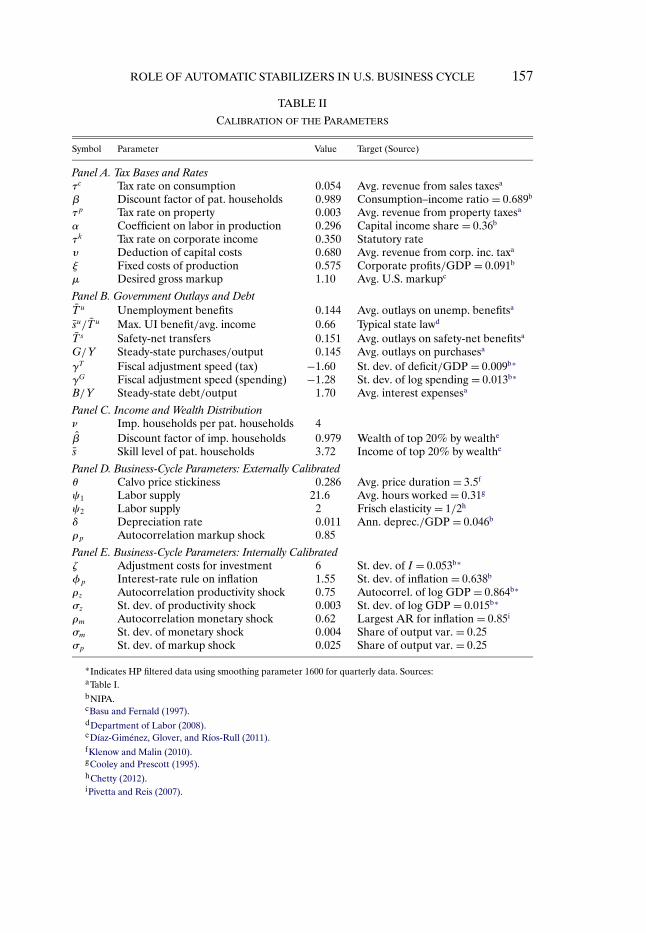
We calibrate as many parameters as possible to the properties of the auto-matic stabilizers in the data. For government spending and revenues, our targetdata are in Table I, which reflects the period 1988–2007. For macroeconomicaggregates, we use quarterly data over a longer period, 1960–2011, so that wecan include more recessions in the sample and periods outside the Great Mod-eration so as not to underestimate the amplitude of the business cycle.15
For the three proportional taxes, we use parameters related to preferencesor technology to match the tax base in the NIPA accounts, and choose the taxrate to match the average revenue reported in Table I, following the strategy
14The method proposed by Reiter (2010) allows for a finer discretization of the distribution ofwealth by using techniques from linear systems theory to compress the state of the model. Wehave used this to verify that our results are not affected by adopting a finer discretization of thedistribution of wealth.
15To ensure that the government’s budget balances in steady state, we scale the outlays thatwe target in our calibration up by 1.024 so that total revenues and outlays are equal in Table I.For example, we calibrate total safety-net spending to be 1.04% of GDP as opposed to 1.02% asappears in Table I.
ROLE OF AUTOMATIC STABILIZERS IN U.S. BUSINESS CYCLE 157
TABLE II
CALIBRATION OF THE PARAMETERS
Symbol Parameter Value Target (Source)
Panel A. Tax Bases and Ratesτc Tax rate on consumption 0�054 Avg. revenue from sales taxesa
β Discount factor of pat. households 0�989 Consumption–income ratio = 0�689b
τp Tax rate on property 0�003 Avg. revenue from property taxesa
α Coefficient on labor in production 0�296 Capital income share = 0�36b
τk Tax rate on corporate income 0�350 Statutory rateυ Deduction of capital costs 0�680 Avg. revenue from corp. inc. taxa
ξ Fixed costs of production 0�575 Corporate profits/GDP = 0�091b
μ Desired gross markup 1�10 Avg. U.S. markupc
Panel B. Government Outlays and DebtT u Unemployment benefits 0�144 Avg. outlays on unemp. benefitsa
su/T u Max. UI benefit/avg. income 0�66 Typical state lawd
T s Safety-net transfers 0�151 Avg. outlays on safety-net benefitsa
G/Y Steady-state purchases/output 0�145 Avg. outlays on purchasesa
γT Fiscal adjustment speed (tax) −1�60 St. dev. of deficit/GDP = 0�009b∗
γG Fiscal adjustment speed (spending) −1�28 St. dev. of log spending = 0�013b∗
B/Y Steady-state debt/output 1�70 Avg. interest expensesa
Panel C. Income and Wealth Distributionν Imp. households per pat. households 4β Discount factor of imp. households 0�979 Wealth of top 20% by wealthe
s Skill level of pat. households 3�72 Income of top 20% by wealthe
Panel D. Business-Cycle Parameters: Externally Calibratedθ Calvo price stickiness 0�286 Avg. price duration = 3�5f
ψ1 Labor supply 21�6 Avg. hours worked = 0�31g
ψ2 Labor supply 2 Frisch elasticity = 1/2h
δ Depreciation rate 0�011 Ann. deprec./GDP = 0�046b
ρp Autocorrelation markup shock 0�85
Panel E. Business-Cycle Parameters: Internally Calibratedζ Adjustment costs for investment 6 St. dev. of I = 0�053b∗
φp Interest-rate rule on inflation 1�55 St. dev. of inflation = 0�638b
ρz Autocorrelation productivity shock 0�75 Autocorrel. of log GDP = 0�864b∗
σz St. dev. of productivity shock 0�003 St. dev. of log GDP = 0�015b∗
ρm Autocorrelation monetary shock 0�62 Largest AR for inflation = 0�85i
σm St. dev. of monetary shock 0�004 Share of output var. = 0�25σp St. dev. of markup shock 0�025 Share of output var. = 0�25
∗Indicates HP filtered data using smoothing parameter 1600 for quarterly data. Sources:aTable I.bNIPA.cBasu and Fernald (1997).dDepartment of Labor (2008).eDíaz-Giménez, Glover, and Ríos-Rull (2011).fKlenow and Malin (2010).gCooley and Prescott (1995).hChetty (2012).iPivetta and Reis (2007).

158 A. MCKAY AND R. REIS
FIGURE 1.—The personal income tax rate from TAXSIM.
of Mendoza, Razin, and Tesar (1994). The top panel of Table II shows theparameter values and the respective targets.
For the personal income tax, we followed Auerbach and Feenberg (2000)and calculated federal and state taxes for a typical household using TAXSIM.We averaged the tax rates across states weighted by population, and acrossyears between 1988 and 2007. We then fit a cubic function of income to the re-sulting schedule, and splined it with a flat line above a certain level of incomeso that the fitted function would be nondecreasing. The result is in Figure 1.The cubic-linear schedule approximates the actual taxes well, and its smooth-ness is useful for the numerical analysis. We then added an intercept to thisschedule to fit the effective average tax rate. This way, we made sure we fit-ted both the progressivity of the tax system (via TAXSIM) and the average taxrates (via the intercept).
Panel B calibrates the parameters related to government spending. Both pa-rameters governing transfer payments are set to match the average outlaysfrom these programs, while the cap on unemployment benefits uses an approx-imation of existing law.
Panel C contains parameters that relate to the distribution of income andwealth across households. According to the Survey of Consumer Finances,83�4% of the wealth is held by the top 20% in the United States (Díaz-

ROLE OF AUTOMATIC STABILIZERS IN U.S. BUSINESS CYCLE 159
Giménez, Glover, and Ríos-Rull (2011)). We then picked the discount factorof the impatient households to match this target.
Omitted from the table for brevity, but available in Appendix A, are theMarkov transition matrices for skill level and employment. We used a three-point grid for household skill levels, which we constructed from data on wagesin the Panel Study for Income Dynamics. The transition matrix across em-ployment status varies linearly with a weighted average of the three aggregateshocks to match the correlation between employment and output. We set itsparameters to match the flows in and out of the two main government transferprograms, food stamps and unemployment benefits, both on average and overthe business cycle.
Finally, Panels D and E have all the remaining parameters. Most are stan-dard, but a few deserve some explanation. First, the Frisch elasticity of laborsupply plays an important role in many intertemporal business-cycle models.Consistent with our focus on taxes and spending, we use the value suggestedin the recent survey by Chetty (2012) on the response of hours worked to sev-eral tax and benefit changes. We have found that the results on the impactof automatic stabilizers on business-cycle volatilities are not very sensitive tothis parameter, although the impact of taxes on the average level of activity isclearly sensitive to the choice of labor supply elasticity. Second, we choose thevariance of monetary shocks and markup shocks so that a variance decompo-sition of output attributes them each 25% of aggregate fluctuations. There isgreat uncertainty on the empirical estimates of the sources of business cycles,but this number is not out of line with some of the estimates in the literature.Our results turn out to not be sensitive to these choices.
Whereas the parameters in Panel D are set directly to match the target mo-ments, those in Panel E (together with β and s in Panel C) are determinedjointly in an internal calibration of the model’s ergodic distribution, that esti-mates these nine parameters to minimize the distance to the nine target mo-ments. While we have tried to use data to discipline our choices of parametersas much as possible, there is nevertheless uncertainty surrounding many of thevalues reported in Table II. A formal estimation and characterization of thisuncertainty is beyond the scope of this study.
3.3. Optimal Behavior and Equilibrium Inequality
Figure 2 uses a simple diagram to describe the stationary equilibrium of themodel without aggregate shocks. For the sake of clarity, the figure depicts anenvironment in which there are no taxes that distort saving decisions.
The downward-sloping curve is the demand for capital, with slope deter-mined by diminishing marginal returns. The supply of savings by patient house-holds is perfectly elastic at the inverse of their time-preference rate just as inthe neoclassical growth model. Because they are the sole holders of capital,the equilibrium capital stock in the model is determined by the intersection

160 A. MCKAY AND R. REIS
FIGURE 2.—Steady-state capital and household bond holdings.
of these two curves. Introducing taxes on capital income, like the personal orcorporate income taxes, raises the pre-tax return on savings that patient house-holds require and lowers the equilibrium capital stock.
If impatient households were also fully insured, their supply of savings wouldbe the horizontal line at β−1. But, because of the idiosyncratic risk they face,they have a precautionary saving motive. Therefore, they are willing to holdbonds at lower interest rates. Their aggregate savings are given by the upward-sloping curve. Because in the steady state without aggregate shocks, bonds andcapital must yield the same return, equilibrium bond holdings by impatienthouseholds are given by the point to the left of the equilibrium capital stock.The difference between the total amount of government bonds outstandingand those held by impatient households gives the bond holdings of patienthouseholds.
Figure 3 shows the optimal savings decisions of impatient households at eachof the employment states. When households are employed, they save, so thepolicy function is above the 45◦ line. When they do not have a job, they rundown their assets. As wealth reaches zero, those out of a job consume all oftheir safety-net income, leading to the horizontal segment along the horizontalaxis in their savings policies.
Figure 4 shows the ergodic wealth distribution for impatient households.Two features of these distributions will play a role in our results. First, manyneedy households hold essentially no assets, so they live hand to mouth. Sec-ond, the figure shows a counterfactual wealth distribution if the two transferprograms are significantly cut. Because not being employed now leads to a

ROLE OF AUTOMATIC STABILIZERS IN U.S. BUSINESS CYCLE 161
FIGURE 3.—Optimal savings policies.
FIGURE 4.—The (smoothed) ergodic wealth distribution (density).

162 A. MCKAY AND R. REIS
TABLE III
FRACTION OF SUBPOPULATION WITH LOW WEALTHa
Skill Level (s)
Employment (e) Share of Population Low Medium High
Employed 0.692 0.574 0.072 0.017Unemployed 0.021 0.589 0.080 0.016Needy 0.087 0.769 0.486 0.334
aLow wealth is defined as assets less than the average quarterly income for an employed household with the sameskill level.
larger loss of income, households save more, which raises their wealth in allstates. Table III shows the proportion of each skill-employment group that hasassets less than one quarter’s average income for an employed individual withthe same skill level.
3.4. Business Cycles
Before we use this model to perform counterfactuals on the effect of theautomatic stabilizers on the business cycle, we inspect whether it can mimicthe key features of U.S. business cycles.
Figure 5 shows the impulse responses to the three aggregate shocks, withimpulses equal to one standard deviation. The model captures the positive co-movement of output, hours, and consumption, as well as the hump-shaped re-sponses of hours to a TFP shock. Inflation rises with expansionary monetaryshocks, but falls with productivity and markup shocks. As usual in the standardCalvo model, the responses are fairly short-lived. In spite of all the heterogene-ity, the aggregate responses to shocks are similar to those of the standard newneoclassical-synthesis model in Woodford (2003) and Christiano, Eichenbaum,and Evans (2005) that has been widely used to study business cycles in the pastdecade.
Turning to the unconditional moments of the business cycle, we chose theparameters of our model so that it mimics the standard deviations of out-put, unemployment, and inflation. Therefore, the model already matches theunconditional second moments in these variables. Also by calibration, themodel already reproduces the main features of the wealth and income dis-tribution.
The marginal propensity to consume (MPC) has received a great deal of at-tention in the study of fiscal policy and it also plays an important role in ourmodel. All else equal, a larger MPC would raise the strength of the disposable-income channel, as any fluctuation in disposable income would translate intoa larger movement in aggregate demand. Moreover, with more heterogeneousMPCs, the redistribution channel will be stronger, as moving resources from

ROLE OF AUTOMATIC STABILIZERS IN U.S. BUSINESS CYCLE 163
FIGURE 5.—Impulse responses to the aggregate shocks.
agents with higher to lower MPCs will have a larger impact on aggregate de-mand.
Table IV shows the distribution of MPCs in our economy according to em-ployment status and wealth percentile. Parker, Souleles, Johnson, and McClel-land (2011) used tax rebates to estimate an average MPC between 0.12 and 0.3.Our model is able to generate MPCs that go from 0.02 to 0.49, so that both inthe spread and on average, it has the potential to give these two channels astrong role. Among the needy and the low-skill unemployed, the MPCs arequite large and more individuals enter these groups in a recession. ComparingTables III and IV, it is clear that the groups with high MPCs are those with fewassets.

164 A. MCKAY AND R. REIS
TABLE IV
MARGINAL PROPENSITY TO CONSUME
Wealth Percentile
Skill Group Employment 10th 25th 50th
Low Employed 0.097 0.079 0.077Medium Employed 0.041 0.035 0.030High Employed 0.030 0.026 0.024
Low Unemployed 0.473 0.339 0.212Medium Unemployed 0.101 0.064 0.048High Unemployed 0.057 0.043 0.034
Low Needy 0.479 0.479 0.478Medium Needy 0.487 0.487 0.097High Needy 0.492 0.130 0.067
3.5. The Effects and Cyclicality of Fiscal Policy
Our calibration strategy targeted the average revenue generated from eachtax. A test of the model is whether it can also match the cyclicality of these rev-enues. Table V reports the covariance of revenues and outlays with detrendedoutput.16 For most spending and tax categories, the model-predicted cyclicali-
TABLE V
COVARIANCE WITH DETRENDED GDPa
Fiscal Variable Data Model
Tax revenues 0�095 0�044Sales tax 0�004 0�007Property tax −0�002 0�003Personal income tax 0�052 0�046Corporate income tax 0�041 −0�013
Purchases −0�009 0�022UI payments −0�020 −0�010Net government savings 0�185 0�136
aQuarterly data from 1960:I–2011:IV and expressed relative to potentialoutput (HP filter trend).
16Detrending is important because the structure of the government budget has changed sig-nificantly across decades, with some sources of revenue and spending growing fast and othersdeclining. We use the HP filter to calculate trend output, and divide both fiscal revenues andoutlays by trend output before calculating the covariance with detrended output. Because thecyclical component of GDP is stationary by construction, by calculating the covariance, we arenot letting the trends in fiscal items affect the estimates. Moreover, by detrending all variablesin the government budget constraint by the common output trend, the covariances of all of theterms in equation (23) have to add up.
ROLE OF AUTOMATIC STABILIZERS IN U.S. BUSINESS CYCLE 165
ties are not only of the right sign but also quite close to their empirical coun-terparts. The main failure is that the model generates countercyclical revenuesfor the corporate income tax while these are strongly procyclical in the data.The reason is that our model, like any new Keynesian model, has counter-cyclical markups. Therefore, because corporate profits are strongly linked tomarkups, the revenue from taxing corporate income is countercyclical in themodel, even though it is procyclical in the data. Overall, the discrepancy be-tween the predicted and actual cyclicality in total tax revenues is 0�051, whichis almost entirely explained by the discrepancy in the cyclicality of corporateincome tax revenue (0.054).
A simple extension of the model can eliminate this gap with little changeto its relevant properties. If only a fraction of the fixed operating cost ξ isdeductible from the corporate income tax and this fraction is countercyclical,then we can exactly match the cyclicality of the corporate income tax revenues.As the fixed cost is not a choice variable, its tax treatment does not changemarginal incentives, so the dynamics of the model barely change. Moreover,we can partially defend this admittedly ad hoc assumption with the limiteddeductibility of corporate income tax credits.
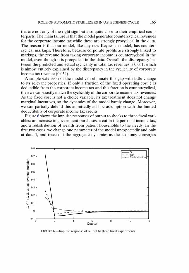
Figure 6 shows the impulse responses of output to shocks to three fiscal vari-ables: an increase in government purchases, a cut in the personal income tax,and a redistribution of wealth from patient households to the needy. In thefirst two cases, we change one parameter of the model unexpectedly and onlyat date 1, and trace out the aggregate dynamics as the economy converges
FIGURE 6.—Impulse response of output to three fiscal experiments.

166 A. MCKAY AND R. REIS
back to its old ergodic distribution. In the third case, we redistribute wealth atdate 1 and simulate the model starting from that new distribution towards theergodic case. In each case, we normalize the response of output by the size ofthe policy change measured in terms of its impact on the government budget.The response to redistribution is nonlinear in the size of the transfer, which weset so that each needy household receives one percent of average householdincome.
Because these shocks have no persistence, their aggregate effect will alwaysbe limited. Yet, we find that they induce relatively large changes in output. Cal-culating multipliers as the ratio of the change in output to the change in thedeficit over the first year of the experiment, we find reasonably sized numbers:0.90 for purchases, 0.27 for taxes, and 0.23 for redistribution. These are largerthan the typical response in the neoclassical-synthesis model. With householdheterogeneity, the aggregate demand effects of these fiscal policies are larger,since the MPC of the needy in particular are very high, and the aggregatesupply effect is larger as well, since the employed households bear more ofthe financing of fiscal expansions, so they are particularly encouraged to workharder when marginal taxes fall or their total after-tax wealth falls. Our modelis therefore able to generate significant effects of fiscal policy.
Figure 7 shows the same responses when we modify the utility function tohave no wealth effects on labor supply as in Greenwood, Hercowitz, and Huff-man (1988). Qualitatively, the responses of output are similar. Quantitatively,the impact of government purchases is larger, since government purchasesraise aggregate demand by more with these preferences, while the impact of
FIGURE 7.—Response of output to fiscal experiments without wealth effect on labor supply.

ROLE OF AUTOMATIC STABILIZERS IN U.S. BUSINESS CYCLE 167
redistribution is smaller, since the employed households no longer choose towork hard as a result of being taxed more heavily. This confirms our intuitionon which economic channels are at work in the model, and provides motivationto consider the quantitative effect that this change will have on our estimatesof the role of the stabilizers.
3.6. Two Special Cases
In the analysis that follows, we consider two special cases of our model asbenchmarks that help isolate different stabilization channels. First, with com-plete markets, households can diversify idiosyncratic risks to their income. Thefollowing assumption eliminates these risks:
ASSUMPTION 1: All households trade a full set of Arrow securities, so they arefully insured, and they are equally patient, β= β.
It will not come as a surprise that if this assumptions holds, there is a rep-resentative agent in this economy. More interesting, the problem she solves isfamiliar:
PROPOSITION 1: Under Assumption 1, there is a representative agent with pref-erences:
maxE0
∞∑t=0
βt{
log(ct)− (1 +Et)ψ1n
1+ψ2t
1 +ψ2
}�
and with the following constraints:
ptct + bt+1 − bt = pt[xt − τ(xt)+ Tnt
]�
xt = It−1
ptbt +wtst(1 +Et)nt + dt + Tut �
st =[
11 +Et s
1+1/ψ2t + Et
1 +Et∫ ν
0s
1+1/ψ2i�t di
]1/(1+1/ψ2)
�
where 1 + Et is total employment, including patient and impatient households,and Tnt is net nontaxable transfers to the household.
The proof is in Appendix B. With the exception of the exogenous shocks toemployment, the problem of this representative agent is fairly standard. More-over, on the firm side, optimal behavior by the goods-producing firms leads toa new Keynesian Phillips curve, while optimal behavior by the capital-goodsfirm produces a familiar IS equation. Therefore, with complete markets, our

168 A. MCKAY AND R. REIS
model is of the standard neoclassical-synthesis variety (Woodford (2003)) thathas been intensively used to study business cycles over the past decade.
The complete-markets case is useful, not just because it is familiar, but alsobecause it allows us to study the effectiveness of automatic stabilizers whendistributional issues are set aside. In this version of the model, the marginalincentives and the disposable income channels are the only two mechanisms atwork.
A second special case that we will consider replaces the impatient house-hold’s optimal savings function with the assumption that all impatient house-holds live hand-to-mouth. That is, they consume all of their after-tax incomeat every date and hold zero bonds. This can be seen as a limit when β ap-proaches zero. It is inspired by the savers–spenders model of Mankiw (2000).In this case, a measure of 80% of all consumers behave as if they were at theborrowing constraint, with an MPC of 1.
This benchmark is useful for several reasons: First, because it is close to theultra-Keynesian model in Gali, Lopez-Salido, and Valles (2007) that combineshand-to-mouth behavior with nominal rigidities to be able to generate a posi-tive multiplier of government purchases on private consumption. For the studyof fiscal policy, this is one of the closest models to the IS-LM benchmark thatis at the center of policy debates on fiscal policy. Second, the assumption ofhand-to-mouth behavior raises the marginal propensity to consume by bruteforce.17 A large MPC, here literally equal to 1 for the impatient households,maximizes the strength of the disposable income channel. Third, in the hand-to-mouth model, there are no precautionary savings so the social insurancechannel is shut off. Our model potentially overstates the role of precautionarysavings as households are infinitely lived and therefore have plenty of time toaccumulate assets. Compared to our full model, the hand-to-mouth alternativeis therefore useful to isolate the channels at work.
4. THE EFFECT OF AUTOMATIC STABILIZERS ON THE BUSINESS CYCLE
To assess whether automatic stabilizers alter the dynamics of the business cy-cle, we calculate the fraction by which the variance of aggregate activity wouldincrease if we removed some, or all, of the automatic stabilizers. If V is theergodic variance at the calibrated parameters, and V ′ is the variance at thecounterfactual with some of the stabilizers shut off, we define, following Smyth(1966), the stabilization coefficient:
S = V ′
V− 1�
17Heathcote (2005) and Kaplan and Violante (2014) raised the MPC in a more elegant wayby, respectively, lowering the discount factor and introducing illiquid assets, but these are hardto accomplish in our model while simultaneously keeping it tractable and able to fit the business-cycle facts and the wealth and income distributions.

ROLE OF AUTOMATIC STABILIZERS IN U.S. BUSINESS CYCLE 169
This differs from the measure of “built-in flexibility” introduced by Pechman(1973), which equals the ratio of changes in taxes to changes in before-tax in-come, and is widely used in the public finance literature.18 Whereas built-inflexibility measures whether there are automatic stabilizers, our goal is insteadto estimate whether they are effective at reducing the volatility of aggregatequantities.
To best understand the difference, consider the following result, proven inAppendix B:
PROPOSITION 2: If Assumption 1 holds, so there is a representative agent, and:1. the Calvo probability of price adjustment θ= 1, so prices are flexible;2. the personal income tax is proportional, so τx(·) is constant;3. the probability of being employed is constant over time;4. there are infinite adjustments costs, γ→ +∞, and no depreciation, δ= 0,
so capital is fixed;5. there are no fixed costs of production, ξ= 0;
then the variance of the log of output is equal to the variance of the log of produc-tivity and S = 0.
While this result and the assumptions supporting it are extreme, it serves auseful purpose. While Assumption 1 shuts off the redistribution and social in-surance channels of stabilization, the other assumptions in Proposition 2 switchoff the aggregate demand channel, since prices are flexible, and the marginalincentives channels, as households and firms face the same marginal taxes inbooms and recessions. The result in Proposition 2 confirms that, in the absenceof these channels, the automatic stabilizers have no effect. Moreover, note thatthe estimates of the size of the stabilizer following the Pechman (1973) ap-proach would be large in this economy. Yet, the stabilizers in this economyhave no impact on the volatility of log output and this is reflected by our ver-sion of the Smyth (1966) measure.
We begin by considering the roles of each of the stabilizers separately. In do-ing so, we set γG = 0 in the fiscal rule so that we show the effect of changing thestabilizers as cleanly as possible without changing the dynamics of governmentpurchases due to the new dynamics for government debt. Because the lump-sum taxes, which are the other means for fiscal adjustment, are approximatelyneutral, they do not risk confusing the effects of the stabilizers with their fi-nancing. We then conduct an experiment of reducing all of the stabilizers atthe same time to calculate the total effect of the automatic stabilizers on thebusiness cycle.
18See Dolls, Fuest, and Peichl (2012) for a recent example, and an attempt to go from built-inflexibility to stabilization, by making the strong assumption that aggregate demand equals outputand that poor households have MPCs of 1 while rich households have MPCs of zero.
170 A. MCKAY AND R. REIS
TABLE VI
THE EFFECT OF PROPORTIONAL TAXES ON THE BUSINESS CYCLEa
Full Model Representative Agent Hand-to-Mouth
Variance Average Variance Average Variance Average
Output −0�0100 0.0117 −0�0019 0.0115 0.0105 0.0116Hours −0�0005 0.0004 0�0029 0.0015 0.0047 0.0006Consumption −0�0098 0.0093 −0�0182 0.0090 0.0400 0.0092
aProportional change caused by cutting the stabilizer.
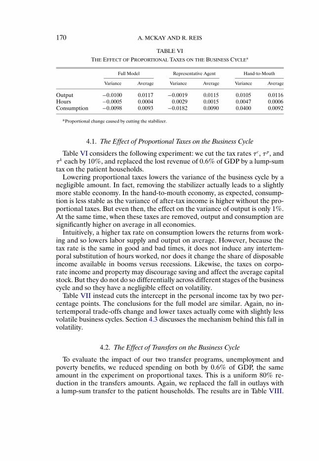
4.1. The Effect of Proportional Taxes on the Business Cycle
Table VI considers the following experiment: we cut the tax rates τc , τp, andτk each by 10%, and replaced the lost revenue of 0�6% of GDP by a lump-sumtax on the patient households.
Lowering proportional taxes lowers the variance of the business cycle by anegligible amount. In fact, removing the stabilizer actually leads to a slightlymore stable economy. In the hand-to-mouth economy, as expected, consump-tion is less stable as the variance of after-tax income is higher without the pro-portional taxes. But even then, the effect on the variance of output is only 1%.At the same time, when these taxes are removed, output and consumption aresignificantly higher on average in all economies.
Intuitively, a higher tax rate on consumption lowers the returns from work-ing and so lowers labor supply and output on average. However, because thetax rate is the same in good and bad times, it does not induce any intertem-poral substitution of hours worked, nor does it change the share of disposableincome available in booms versus recessions. Likewise, the taxes on corpo-rate income and property may discourage saving and affect the average capitalstock. But they do not do so differentially across different stages of the businesscycle and so they have a negligible effect on volatility.
Table VII instead cuts the intercept in the personal income tax by two per-centage points. The conclusions for the full model are similar. Again, no in-tertemporal trade-offs change and lower taxes actually come with slightly lessvolatile business cycles. Section 4.3 discusses the mechanism behind this fall involatility.
4.2. The Effect of Transfers on the Business Cycle
To evaluate the impact of our two transfer programs, unemployment andpoverty benefits, we reduced spending on both by 0�6% of GDP, the sameamount in the experiment on proportional taxes. This is a uniform 80% re-duction in the transfers amounts. Again, we replaced the fall in outlays witha lump-sum transfer to the patient households. The results are in Table VIII.

ROLE OF AUTOMATIC STABILIZERS IN U.S. BUSINESS CYCLE 171
TABLE VII
THE EFFECT OF THE LEVEL OF TAX RATES ON THE BUSINESS CYCLEa
Full Model Representative Agent Hand-to-Mouth
Variance Average Variance Average Variance Average
Output −0�0051 0.0078 −0�0127 0.0076 −0�0600 0.0075Hours −0�0140 0.0036 −0�0090 0.0076 −0�0155 0.0034Consumption −0�0203 0.0089 −0�0142 0.0087 −0�0264 0.0086
aProportional change caused by cutting the stabilizer.
Transfers have a close-to-zero effect on the average level of output and hours,yet they have a substantial effect on their volatility. Reducing transfer pay-ments raises output volatility by 6% and raises the variance of hours workedby as much as 9%.
Aside from the social-insurance channel, there is also a redistribution chan-nel behind the impact of transfers on aggregate volatility. In a recession, thereare more households without a job so more transfers in the aggregate. Trans-fers have no direct effect on the labor supply of recipients as they do not havea job in the first place. However, they are funded by higher taxes on the patienthouseholds, who raise their hours worked in response to the reduction in theirwealth. This stabilizes hours worked and output.
At the same time, without transfers, the volatility of aggregate consumptionfalls by 1%. To understand why, note that the transfers provide social insuranceagainst a major idiosyncratic shock that impatient households face. As house-holds face more risk without transfers, they accumulate more assets. This wasvisible in Figure 4, with the large shift of the wealth distribution to the rightwhen transfers are reduced. With more savings, impatient households are bet-ter able to smooth their consumption in response to fluctuations in incomecaused by aggregate shocks and aggregate consumption becomes more stable.
The two special cases also confirm that redistribution and precautionary sav-ings are behind the effectiveness of transfers. In the representative-agent econ-omy, both of these channels are shut off, and the transfer experiment has a
TABLE VIII
THE EFFECT OF TRANSFERS ON THE BUSINESS CYCLEa
Full Model Representative Agent Hand-to-Mouth
Variance Average Variance Average Variance Average
Output 0�0603 −0�0004 −0�0063 0.0002 −0�0083 −0�0042Hours 0�0944 −0�0098 −0�0037 0.0002 0�0047 −0�0017Consumption −0�0133 −0�0004 −0�0119 0.0002 0�1003 −0�0048
aProportional change caused by cutting the stabilizer.

172 A. MCKAY AND R. REIS
negligible effect on all variables. In the hand-to-mouth economy, eliminatingthe public insurance provided by transfers raises the volatility of aggregate con-sumption. This is as expected, since a large fraction of the population does notsmooth their consumption. Nonetheless, the volatility of output now slightlyfalls without transfers. The hand-to-mouth economy maximizes the disposable-income channel since every dollar given to impatient households is spent, rais-ing output because of sticky prices. Yet, we see that, quantitatively, this effectaccounts for little of the stabilizing effects of transfers in our economy.
This intuition also suggests that the effectiveness of transfers relies on a posi-tive wealth effect on labor supply. When we repeated the same experiment withpreferences without this wealth effect, the variance of output then increases bymore, 11�4%, without the stabilizers, while the variance of consumption nowincreases as well, by 6�6%, in contrast with the results in Table VIII. The in-tuition is as follows. Under standard preferences, households use labor supplyas a form of precautionary insurance. In a recession, the increase in unem-ployment risk induces them to not only consume less but also to increase laborsupply in order to accumulate additional savings. With Greenwood, Hercowitz,and Huffman (1988) preferences, the household responds to changes in riskonly through consumption, not labor supply. Therefore, consumption and ag-gregate demand must change by more, and transfers become more effective.19
By taking the unemployment rate to be exogenous, our analysis does notincorporate the impact of aggregate demand stabilization on the extent of id-iosyncratic risk. This channel has been studied extensively by Ravn and Sterk(2013). Conversely, by taking the unemployment rate to be exogenous, ouranalysis does not incorporate the disincentive effect of unemployment ben-efits on the incentive for unemployed workers to engage in costly search, asin Young (2004), or for workers to accept lower wages when employed, as inHagedorn, Karahan, Manovskii, and Mitman (2013).20
4.3. The Effect of Progressive Income Taxes on the Business Cycle
Our next experiment replaces the progressive personal income tax with aproportional, or flat, tax that raises the same revenue in steady state. Table IXhas the results.
Progressive income taxes have a modest effect on the volatility of output orhours, but moving to a flat tax would raise the average level of economic activ-ity significantly, with output and consumption increasing by 4%. This stands in
19The importance of wealth effects for the effectiveness of transfers has recently been empha-sized by Athreya, Owens, and Schwartzman (2014). Yet, there is no empirical consensus on howlarge this wealth effect is.
20An earlier version of this paper considered an extension of the model that captures the dis-incentive effects of transfers. Results are available from the authors upon request.

ROLE OF AUTOMATIC STABILIZERS IN U.S. BUSINESS CYCLE 173
TABLE IX
THE EFFECT OF PROGRESSIVE TAXES ON THE BUSINESS CYCLEa
Full Model Representative Agent Hand-to-Mouth
Variance Average Variance Average Variance Average
Output 0�0023 0.0446 −0�0565 0.0383 −0�1484 0.0466Hours −0�0147 0.0388 −0�0189 0.0383 −0�0541 0.0316Consumption −0�0665 0.0507 −0�0013 0.0436 0�0167 0.0531
aProportional change caused by cutting the stabilizer.
contrast to our results for transfers, even though both are redistributive poli-cies. To understand this difference, we can consider the four channels we dis-cussed in the Introduction.
First, because marginal tax rates rise with income, this discourages laborsupply and lowers average hours and investment, leading to reduced aver-age income. This well-understood mechanism works in the cross-section, dis-couraging individual households from trying to raise their individual income.However, the level of progressivity in the current U.S. tax system is modestin the sense that the marginal tax rate function is relatively flat above medianincome—recall Figure 1. Therefore, the marginal tax rate that many employedhouseholds face changes little between booms and recessions. This induces lit-tle substitution over time, and therefore has a negligible effect on the variance.
On average activity, though, the effect is large. With a flat tax, becausemore tax revenue is collected from households with less income, then the high-income households face a significantly lower marginal tax rate. Therefore, theysave more, the average capital stock is higher, and so the impact of flatteningthe tax system on average income is large.
Second, the redistribution channel is significantly weaker than with trans-fers, because it is less targeted. When the needy receive transfers, they can-not reduce their labor supply any further. In contrast, the personal income taxmostly redistributes among employed households. The recipients lower theirlabor supply in response to their higher income, and little stabilization results.
The important roles of redistribution and precautionary savings are againhighlighted by the two special cases, where these two channels are shut off.The table shows that in either the representative-agent or the hand-to-moutheconomies, a flat tax leads instead to significantly less volatile business cycles.Further calculations, that we do not report for brevity, show that this fall involatility is in large part driven by the joint presence of monetary policy shocksand sticky prices.
To understand what is going on, recall the basic mechanism for why a positivemonetary policy shock causes a boom with sticky prices: lower nominal interestrates lead to lower real interest rates, which raises consumption, demand foroutput, and if prices do not change, then raises hours worked and investment.
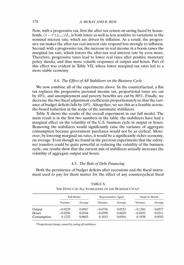
174 A. MCKAY AND R. REIS
Now, with a progressive tax, first the after-tax return on saving faced by house-holds, (1 − τx(xt+1))It , is both lower as well as less sensitive to variations in thenominal interest rate, which are driven by inflation. As a result, the progres-sive tax makes the after-tax real interest rate respond less strongly to inflation.Second, with a progressive tax, the increase in real income in a boom raises themarginal tax rate, which lowers the after-tax real interest rate by even more.Therefore, progressive taxes lead to lower real rates after positive monetarypolicy shocks, and thus more volatile responses of output and hours. Part ofthis effect was evident in Table VII, where lower marginal tax rates led to amore stable economy.
4.4. The Effect of All Stabilizers on the Business Cycle
We now combine all of the experiments above. In the counterfactual, a flattax replaces the progressive personal income tax, proportional taxes are cutby 10%, and unemployment and poverty benefits are cut by 80%. Finally, wedecrease the two fiscal adjustment coefficients proportionately so that the vari-ance of budget deficits falls by 10%. Altogether, we see this as a feasible across-the-board reduction in the scope of the automatic stabilizers.
Table X shows the results of the overall experiment in our full model. Themain result is in the first two numbers in the table: the stabilizers have had amarginal effect on the volatility of the U.S. business cycle in output or hours.Removing the stabilizers would significantly raise the variance of aggregateconsumption because government purchases would not be as cyclical. More-over, by lowering marginal tax rates, it would be a significantly richer economy,on average. Even though we found in the previous experiments that the safety-net transfers could be quite powerful at reducing the volatility of the businesscycle, our results show that the current mix of stabilizers actually increases thevolatility of aggregate output and hours.
4.5. The Role of Debt Financing
Both the persistence of budget deficits after recessions and the fiscal instru-ment used to pay for them matter for the effect of any countercyclical fiscal
TABLE X
THE EFFECT OF ALL STABILIZERS ON THE BUSINESS CYCLEa
Full Model Representative Agent Hand-to-Mouth
Variance Average Variance Average Variance Average
Output −0�0229 0.0567 −0�0756 0.0533 −0�1381 0.0557Hours −0�0296 0.0344 −0�0399 0.0429 −0�0432 0.0311Consumption 0�1232 0.0603 0�1833 0.0564 0�1938 0.0593
aProportional change caused by cutting all stabilizers.
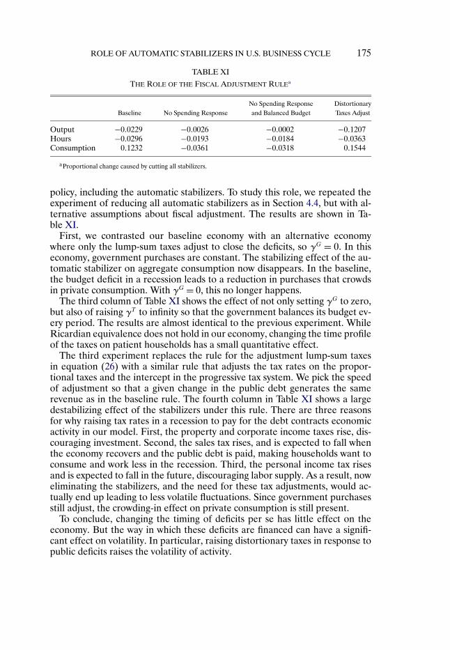
ROLE OF AUTOMATIC STABILIZERS IN U.S. BUSINESS CYCLE 175
TABLE XI
THE ROLE OF THE FISCAL ADJUSTMENT RULEa
No Spending Response DistortionaryBaseline No Spending Response and Balanced Budget Taxes Adjust
Output −0�0229 −0�0026 −0�0002 −0�1207Hours −0�0296 −0�0193 −0�0184 −0�0363Consumption 0�1232 −0�0361 −0�0318 0�1544
aProportional change caused by cutting all stabilizers.
policy, including the automatic stabilizers. To study this role, we repeated theexperiment of reducing all automatic stabilizers as in Section 4.4, but with al-ternative assumptions about fiscal adjustment. The results are shown in Ta-ble XI.
First, we contrasted our baseline economy with an alternative economywhere only the lump-sum taxes adjust to close the deficits, so γG = 0. In thiseconomy, government purchases are constant. The stabilizing effect of the au-tomatic stabilizer on aggregate consumption now disappears. In the baseline,the budget deficit in a recession leads to a reduction in purchases that crowdsin private consumption. With γG = 0, this no longer happens.
The third column of Table XI shows the effect of not only setting γG to zero,but also of raising γT to infinity so that the government balances its budget ev-ery period. The results are almost identical to the previous experiment. WhileRicardian equivalence does not hold in our economy, changing the time profileof the taxes on patient households has a small quantitative effect.
The third experiment replaces the rule for the adjustment lump-sum taxesin equation (26) with a similar rule that adjusts the tax rates on the propor-tional taxes and the intercept in the progressive tax system. We pick the speedof adjustment so that a given change in the public debt generates the samerevenue as in the baseline rule. The fourth column in Table XI shows a largedestabilizing effect of the stabilizers under this rule. There are three reasonsfor why raising tax rates in a recession to pay for the debt contracts economicactivity in our model. First, the property and corporate income taxes rise, dis-couraging investment. Second, the sales tax rises, and is expected to fall whenthe economy recovers and the public debt is paid, making households want toconsume and work less in the recession. Third, the personal income tax risesand is expected to fall in the future, discouraging labor supply. As a result, noweliminating the stabilizers, and the need for these tax adjustments, would ac-tually end up leading to less volatile fluctuations. Since government purchasesstill adjust, the crowding-in effect on private consumption is still present.
To conclude, changing the timing of deficits per se has little effect on theeconomy. But the way in which these deficits are financed can have a signifi-cant effect on volatility. In particular, raising distortionary taxes in response topublic deficits raises the volatility of activity.

176 A. MCKAY AND R. REIS
5. MONETARY POLICY AND AUTOMATIC STABILIZERS
Our results show that the automatic stabilizers have overall little effect onthe dynamics of the business cycle. In particular, the usual arguments about thebenefits of the stabilizers in aggregate demand management are not supportedby our findings. There are two ways we could have arrived at this conclusion.One possibility is that the model might attribute little importance to aggregatedemand management in general. In this section, we argue that this is not thecase. Instead, we argue that monetary policy comes close to reaching the firstbest already, so there is little additional role for fiscal policy. We then showthat when monetary policy is far from optimal, the automatic stabilizers havean important stabilizing effect.
5.1. The Roles of Price Stickiness and Monetary Policy
Figure 5 already showed that shocks to monetary policy have a significanteffect on output in our economy. According to the model, a 25 basis pointunexpected increase in interest rates lowers output on impact by 0.3%. Whilethe aggregate demand channel of fiscal policy is weak, monetary policy stillplays a significant role in the economy.
Table XII repeats the experiment of reducing all the stabilizers in our modelunder different assumptions about monetary policy. First, a useful bench-mark is the case where prices are fully flexible, and it is shown in the sec-ond column of the table. This eliminates the role of monetary policy en-tirely and neutralizes the aggregate demand channel. A common finding inthe representative-agent version of our business-cycle model without taxes andtransfers is that a finely tuned monetary policy can come close to reaching thefirst best (Woodford (2003)). We explore this in the third column of the table,which shows the same experiment with sticky prices but now with a mone-tary policy rule that Schmitt-Grohé and Uribe (2007) showed is close to op-timal in a version of the Christiano, Eichenbaum, and Evans (2005) model:log(It/It−1)= 0�77 log(It−1/It−2)+0�75 log(πt−1)+0�02 log(yt−1/yt−2). This rule
TABLE XII
THE EFFECT OF ALL STABILIZERS WITH DIFFERENT MONETARY POLICIESa
Taylor Rule
Flexible Prices S.G.-U. Baseline Output Aggressive Accommodative
Output −0�0428 −0�0430 −0�0229 −0�0333 −0�0339 0.1435Hours −0�0390 −0�0408 −0�0296 −0�0116 −0�0172 0.0891Consumption 0�1165 0�1256 0�1232 0�0905 0�0898 0.0016Inflation −0�4123 −0�2907 −0�2828 0�0822 0�0436 0.5201
aProportional change caused by cutting the stabilizer.

ROLE OF AUTOMATIC STABILIZERS IN U.S. BUSINESS CYCLE 177
has the virtue of depending only on observables, so it avoids the difficulty ofdefining the right concept of the output gap. The impact of the stabilizers isvery similar to the flexible-price case. This confirms the conjecture that with aneffective monetary policy, there is little room left for the automatic stabilizersto work through aggregate demand.
The last three columns of our table consider different versions of a Taylorrule that sets the expected after-tax interest rate as a function of the currentinflation rate:21
Et
[1 − τx(xt+1)
]It = I +φp� log(pt)+φy� log(yt)− εt�(28)
Focusing monetary policy on the after-tax interest rate makes the analysis moretransparent because, as we explained at the end of Section 4.3, the progressiveincome tax interacts with the monetary policy rule to determine the effectiveresponse of real interest rates to inflation.22 With this after-tax rule, the inter-pretation of φp is closer to the more familiar case without taxes on interest in-come. Varying φp and φy lets us study the effect of more aggressive responsesof monetary policy to inflation, and of responding to output as well, respec-tively.
The aggressive policy rule setsφp = 1�75 whereas our baseline hasφp = 1�55,both with φy = 0. The output policy rule has φp = 1�55 as in the baseline butnow φy = 0�125. In all three cases, the results are similar to the flexible-pricebenchmark.
The accommodative policy rule sets φp = 1�03, so the after-tax real inter-est rate is quite insensitive to changes in inflation. Under such a rule, demandshocks will lead to larger fluctuations in activity, as they are not offset by mon-etary policy. In contrast to the other cases, here we find that the automaticstabilizers have an important role in stabilizing output and hours. Under theaccommodative policy, the stabilizers have little effect on the volatility of ag-gregate consumption. This makes sense, as the strong effect of the stabilizerson aggregate consumption in the baseline arose out of changes in the dynamicsof government purchases. With an accommodative monetary policy, however,private consumption is insulated from changes in the dynamics of governmentpurchases.
To sum up, the rules that either approximate the U.S. data, or are optimal ina related model, or are particularly aggressive, all seem to effectively manageaggregate demand, leaving little room for fiscal policy. But with the accom-modative rule, the stabilizers substantially reduce the volatility of aggregateoutput and hours.
21We use the expected tax-rate of the patient households in this rule.22That a constant tax on interest income alters the effective monetary policy rule was previously
noted by Edge and Rudd (2007). In our model, this effect is larger due to the progressivity of thetax system.

178 A. MCKAY AND R. REIS
5.2. Automatic Stabilizers at the Zero Lower Bound
One situation where monetary policy is very accommodative is when nominalinterest rates are at the zero lower bound (ZLB). At the same time, muchrecent research has shown that fiscal policy can be particularly powerful whennominal interest rates do not respond to inflation (Woodford (2011)), and thatdifferent fiscal instruments can have widely different impacts relative to eachother and to the case where the Taylor principle holds (Eggertsson (2011)).Given the often paradoxical results that the literature has found at the ZLB, itis not clear how the role of the automatic stabilizers might change.
At the same time, it is not easy to solve our model when the ZLB binds.For one, most algorithms rely on the ZLB being a current state that will neverrepeat itself in the future (Eggertsson and Woodford (2003)), whereas our fo-cus has been on the ergodic steady state. Second, we have to solve the modelnonlinearly to capture the important precautionary savings and social insur-ance channels, but nonlinear solution algorithms for economies at the ZLBare still in their infancy and cannot solve models as large as ours (Fernandez-Villaverde, Gordon, Guerron, and Rubio-Ramirez (2014)). Third, hitting theZLB and staying there for more than one period is difficult in models withrealistic capital adjustment costs, because of the investment boom that comeswith low interest rates (Christiano, Eichenbaum, and Rebelo (2011)).
To solve these problems, we make the following simplifications. First, we setthe capital adjustment cost to infinity so that the capital stock is fixed. Second,and related, we raise the degree of price stickiness to θ= 0�15, still in line withsome empirical estimates, because this helps ensure the existence of a deter-minate equilibrium.23 Third, instead of the ergodic distribution, we calculate aperfect foresight transition path starting from a stationary equilibrium at date0 where there are no aggregate shocks but households still face idiosyncraticuncertainty. We found it necessary to make these simplifications in order toincorporate the strong nonlinearities at the ZLB, but this comes at a cost ofeliminating investment and aggregate uncertainty, both of which could haveimportant consequences for the quantitative results.
At date 1, everyone learns that the rate of time preference of all householdsfalls by 0.25% for 15 periods, a standard shock in the ZLB literature.24 More-over, at the same time, the risk of becoming unemployed rises by 1.35% perquarter and the job-finding rate of needy households falls by 0.89% for 8 quar-ters, so that we generate a cumulative drop in employment of 4%, close tothe peak-to-trough decline in employment during the U.S. Great Recession.
23We verified that the results in the paper so far do not change much with this new value for θ.Increasing price stickiness helps dampen the explosive dynamics of inflation at the zero lowerbound by having fewer firms update their prices and by making current inflation depend moreheavily on future inflation and less on current marginal costs.
24Specifically, the discount factors β and β both rise by a factor of 1.0025.

ROLE OF AUTOMATIC STABILIZERS IN U.S. BUSINESS CYCLE 179
FIGURE 8.—The zero lower bound episode with and without automatic stabilizers.
Appendix G of the Supplemental Material explains how we construct an equi-librium transition path.
The solid lines in Figure 8 show the dynamics of the nominal interest rate,output, aggregate consumption, and the total consumption of impatient house-holds. The zero lower bound binds for the first two periods of the transitionbefore gradually returning to its steady-state value. Aggregate consumptiondrops by 6% on impact, and output by 4%. Impatient households are partic-ularly affected by the deterioration in labor market conditions, so their con-sumption drops by nearly 10% on impact. The dashed lines in the figure showthe economy’s response to the same set of shocks when all stabilizers have beenreduced as in our baseline experiment. The impact of the shock is now substan-tially larger. The ZLB binds for a further period, and consumption and outputfall by an additional 2% and 1%, respectively. With the reduction of social in-surance, impatient households are hurt even more, and their consumption fallsby an additional 5%, for a total fall of 15%.
These results suggest that the automatic stabilizers are more effective in mit-igating the extent of the contraction during a zero lower bound episode. This

180 A. MCKAY AND R. REIS
finding is consistent with other studies of the power of fiscal policy at the zerolower bound (e.g., Christiano, Eichenbaum, and Rebelo (2011)).
6. THE WELFARE EFFECTS OF AUTOMATIC STABILIZERS
The automatic stabilizers affect welfare partly due to their impact on the am-plitude of the business cycle that we have focused on so far. At the same time,they also affect welfare by changing the average level of activity or the extentof public insurance that they provide against idiosyncratic risks. This sectiondiscusses these different effects on welfare to answer whether the stabilizersare desirable from a welfare perspective.
6.1. The Overall Welfare Consequences of Automatic Stabilizers
Table XIII shows the change in the welfare of different agents in our econ-omy from reducing all the stabilizers as in the experiment in Section 4.4. Inthis calculation, we consider taking a household with their current individualstate variables from the economy with stabilizers and placing them into theeconomy without stabilizers. We take both economies to be at their respectivesteady states, but the welfare of the agents reflects the anticipation of fluctua-tions going forward. In the table, an entry of −0�10 indicates that a householdhas lower welfare without the stabilizers by an amount equivalent to 10% ofconsumption.
As shown in the table, all impatient households are worse off in the worldwithout stabilizers. The equally weighted average welfare loss in the table is−0�151. The welfare of the patient households, in contrast, increases by 0.136.The stabilizers have a large redistributive component, so a policy of scaling
TABLE XIII
WELFARE COST TO IMPATIENT HOUSEHOLDS OF REDUCING AUTOMATIC STABILIZERSa
Wealth Percentile
Employment Skill 10th 25th 50th 75th 90th
Employed Low −0�174 −0�173 −0�173 −0�167 −0�156Employed Medium −0�139 −0�136 −0�133 −0�127 −0�123Employed High −0�101 −0�099 −0�097 −0�096 −0�096
Unemployed Low −0�253 −0�244 −0�240 −0�217 −0�190Unemployed Medium −0�200 −0�185 −0�172 −0�155 −0�144Unemployed High −0�142 −0�131 −0�123 −0�118 −0�116
Needy Low −0�371 −0�371 −0�371 −0�336 −0�266Needy Medium −0�354 −0�354 −0�282 −0�230 −0�194Needy High −0�334 −0�271 −0�198 −0�166 −0�152
aWelfare expressed in the proportional change caused in consumption equivalent of cutting all stabilizers.

ROLE OF AUTOMATIC STABILIZERS IN U.S. BUSINESS CYCLE 181
down transfers and moving to a flat tax benefits the rich patient householdsand hurts the poor impatient households. Across impatient households, it isalso clear that the policy change has large redistributive effects. The low-wealthneedy lose particularly large amounts, as they are entirely reliant on trans-fers for their current consumption. These disparate effects make it hard tostate whether the stabilizers are beneficial or not. One controversial answeris to take a utilitarian social welfare function that weighs each group by theirpopulation; in this case, cutting the stabilizers lowers average welfare by 0.080consumption-equivalent units.
The numbers in the table compare ergodic distributions. However, one ofthe reasons why average output in the economy is higher without stabilizers isthat households face higher risk and raise their precautionary savings. Thesecome at the expense of lower consumption in the transition, so ignoring thistransition may lead to an underestimate of the welfare benefits of the stabi-lizers. Yet, when we calculated the welfare of agents from the moment of thepolicy change onwards, we found that the welfare estimates are only slightlylower than in Table XIII.
The welfare changes in the table are large for two complementary reasons:first, because the stabilizers are providing social insurance, which the uninsuredimpatient households benefit from; second, because the stabilizers change theaverage level of post-tax income among different types of households, redis-tributing resources even in the absence of shocks.
6.2. Isolating the Impact of Recessions
Another difficulty with assessing the effect of the stabilizers in welfare is thatmost of their benefits have little to do with the business cycle. Social insurancemay be desirable and useful, regardless of whether it leads to business cyclesthat are more, less, or similarly volatile. To investigate this, we now look at theeffect of the stabilizers during a recession.
In particular, we compute the welfare cost of a series of recessions with andwithout the stabilizers. We consider four recessionary episodes: a two standarddeviation drop in TFP, a two standard deviation contractionary monetary pol-icy shock, a two standard deviation inflationary markup shock, and the zerolower bound episode described in Section 5.2. For each, we compute a perfectforesight transition for 250 quarters and the utility of agents at the momentthe shock is realized. We then compare this utility to the case without shocksin which the economy will remain at the steady state. This gives us the welfarecost of these recessions. Table XIV shows the results.
With any of the shocks that we consider for our baseline model, the costof business cycles is small. As noted by Lucas (1987), this is a general featureof business cycle models, and ours is no different. The exception is the ZLB,where the costs are close to 3% of consumption.
More interesting, without the stabilizers, there is a large increase in the wel-fare cost of the recessions in relative terms. Without stabilizers, the extra risk

182 A. MCKAY AND R. REIS
TABLE XIV
UTILITARIAN COST OF RECESSIONS
Shock Cost With Stabilizers Cost Without Stabilizers Difference
Technology −0�00092 −0�00365 −0�00272Monetary policy −0�00227 −0�00258 −0�00031Markups −0�00206 −0�00363 −0�00157Zero Lower Bound −0�02964 −0�03554 −0�00590
of ending up in the needy state during a recession episode can be quite costly tothe impatient agents, who, in anticipation, have lower expected welfare. How-ever, comparing the results from Table XIV to the welfare consequences in Ta-ble XIII, we see that the large welfare costs of eliminating the stabilizers werenot due to business cycles. From the narrow business-cycle perspective of thispaper, the stabilizers play a large role on how costly business cycles are. But,overall, these are not very costly to start with, so the benefit is small. Rather,the large welfare benefits of the stabilizers are due to redistribution and socialinsurance, not business-cycle fluctuations.
7. CONCLUSIONS AND FUTURE WORK
Milton Friedman (1948) famously railed against the use of discretionary pol-icy to stabilize the business cycle. He defended the power instead of fiscal auto-matic stabilizers as a preferred tool for countercyclical policy. More recently,Solow (2005) strongly argued that policy and research should focus more onautomatic stabilizers as a route through which fiscal policy could and shouldaffect the business cycle.
We constructed a business-cycle model with many of the stabilizers and cal-ibrated it to replicate the U.S. data. The model has some interesting featuresin its own right. First, it nests both the standard incomplete-markets model, aswell as the standard new-Keynesian business-cycle model. Second, it matchesthe first and second moments of U.S. business cycles, as well as the broad fea-tures of the U.S. wealth and income distributions. Third, solving it requiresusing new methods that may be useful for other models that combine nominalrigidities and incomplete markets.
We found that lowering taxes on sales, property, and corporate and personalincome, or reducing the progressivity of the personal income tax, did not havea significant impact on the volatility of the business cycle. Moreover, loweringthese taxes raised average output. At the same time, higher transfers to the un-employed and poor were quite effective at lowering the volatility of aggregateoutput.
In terms of the channels of stabilization, we found that the traditionaldisposable-income channel used to support automatic stabilizers is quantita-

ROLE OF AUTOMATIC STABILIZERS IN U.S. BUSINESS CYCLE 183
tively weak. Considerably more important was the role of precautionary sav-ings and social insurance. Moreover, both because of the role of precautionarysavings and because of the changes in government purchases to pay for pub-lic debt, the stabilizers can, at the same time, stabilize aggregate consumption,while destabilizing aggregate output.
Overall, we found that reducing the scope of all the stabilizers would havehad little impact on the volatility of the U.S. business cycle in the last decades.This depends on monetary policy having responded aggressively to inflationand being close to optimal. When monetary policy is far from optimal, the au-tomatic stabilizers play a useful role in reducing the magnitude of the businesscycle, and during the recent episode with the zero lower bound, they may havesignificantly reduced the depth of the recession. Nearly all of the welfare im-pact of reducing the stabilizers comes from the social insurance they provide,and not from their impact on the business cycle.
Aside from monetary policy, labor market institutions and policies also likelymatter for our results. In our model, we assume that transitions across employ-ment states are exogenous, but this ignores the disincentive effects of transfersto those without a job on engaging in costly job search (e.g., Young (2004)) orin accepting lower wage offers (e.g., Hagedorn et al. (2013)). We have exploredthis in a version of the model where the probability of finding a job dependedon search effort, which in turn lowered leisure of unemployed households. Asexpected, stabilizers were even less effective, and more consistently destabiliz-ing, as the increase in transfers to the unemployed during a recession lowerstheir search effort and prolongs the recession.25 Finally, Ravn and Sterk (2013)highlighted an alternative interaction coming from labor demand, as unem-ployment risk leads to precautionary savings, which lowers aggregate demand,reduces hiring, and so causes more unemployment risk. Like us, they foundthat aggressive monetary policy is very effective at dealing with this channel.Considering these and other interactions between the stabilizers and labor sup-ply and demand seems a fruitful area for more research.
Another area for future work is the optimal design of stabilizers. Before do-ing so, we had to understand the positive predictions of the model regardingthe stabilizers, a task that occupies this whole paper. Future work can take upthe challenge of optimal policy design. Being able to do this work in a quanti-tative model like the one in this paper will have to overcome some challengingcomputational hurdles.
Finally, each of the automatic stabilizers that we considered is more com-plex than our description and distorts behavior in more ways than the ones wemodeled. Here we have sought to incorporate the most important channelsthrough which the stabilizers could work while omitting other features of the
25All of these experiments are available from the authors, or are in the working paper versionof this paper.

184 A. MCKAY AND R. REIS
economy in order to keep the model tractable. To obtain a sharper quantita-tive estimate of the role of the stabilizers, it would be desirable to include thefindings from the rich micro literatures that study each of these governmentprograms in isolation. Perhaps the main point of this paper is that to assess au-tomatic stabilizers requires having a fully articulated business-cycle model, sothat we can move beyond the disposable-income channel, and consider otherchannels as well as quantify their relevance. Our hope is that as computationalconstraints diminish, we can keep this macroeconomic approach of solving forgeneral equilibrium, while being able to consider the richness of the microdata.
APPENDIX A: CALIBRATION OF THE IDIOSYNCRATIC SHOCK PROCESSES
Each household at every date has a draw of st(i) determining the wage theyreceive if they are employed, and a draw of et(i) on their employment status.This section describes how we calibrate the distribution and dynamics of thesetwo random variables.
A.1. Skill Shocks
We use PSID data on wages to calibrate the skill process. To do this, we startwith sample C from Heathcote, Perri, and Violante (2010) and work with thelog wages of household heads in years 1968 to 2002. Computational consid-erations limit us to three skill levels, and we construct a grid by splitting thesample into three groups at the 33rd and 67th percentiles and then using themedian wage in each group as the three grid points, which results in skill levelsof 0�50, 0�92, and 1�64.26 Skills are proportional to the level (not log) of thesewages. Computational considerations also lead us to choose a skill transitionmatrix with as few nonzero elements as possible. We impose the structure(1 −p p 0
p 1 − 2p p0 p 1 −p
)�
where p is a parameter that we calibrate as follows. From the PSID data, wecompute the first, second, and fourth autocovariances of log wages. Let Γi bethe ith autocovariance. We use the moments Γ2/Γ1 and
√Γ4/Γ2, each of which
can be viewed as an estimate of the autoregressive parameter if the log wagesfollow an AR(1) process.27 The empirical moments are 0�9356 and 0�9496, re-spectively. To map these moments into a value of p, we minimize the equally
26The overall scale of skills is normalized so that average income in the economy is equal to 1.27The ratio Γ1/Γ0 is not used, as this ratio is heavily influenced by measurement error, which
leads to an underestimate of the persistence of wages. The moments that we use were also usedby Heathcote, Storesletten, and Violante (2010) to estimate the persistence of the wage process.

ROLE OF AUTOMATIC STABILIZERS IN U.S. BUSINESS CYCLE 185
weighted sum of squared deviations between these empirical moments andthose implied by the three-state Markov chain. As our time period is one quar-ter, while the PSID data are annual, we use Γ8/Γ1 and
√Γ16/Γ8 from the model.
This procedure results in a value of p of 0.015.
A.2. Employment Shocks
Steady State
In addition to differences in skill levels, households differ in their employ-ment status. A household can be (1) employed (E), (2) unemployed (U), or(3) needy (N). To construct a steady-state transition matrix between these threestates, we need six moments. First, it is reasonable to assume that a house-hold does not transit directly from employed to long-term unemployed or fromlong-term unemployed back to unemployed. Those two elements of the transi-tion matrix are therefore set to zero.
The distribution of households across states gives us two more moments. Asthe focus of our work is on the level and fluctuation in the number of individu-als receiving different types of transfers, we define unemployed as individualswho are receiving unemployment benefits and needy as those receiving foodstamps.
In the United States, the Supplemental Nutritional Assistance Program(SNAP) is the largest nonhealth, nonretirement social safety net program.SNAP assists low-income households in being able to purchase a minimally ad-equate low-cost diet. Recipients of these benefits are generally not working.28
One virtue of using SNAP participation as a proxy for long-term unemploy-ment is that it avoids the subtle distinction between unemployment and non-participation in the Current Population Survey while still focusing on thoseindividuals who likely have poor labor market prospects. If we instead usedtime since last employment to identify those in long-term unemployment, wewould include a number of individuals with decent opportunities to work ifthey chose to do so, such as individuals who have retired or who choose towork in the home. Between 1971, when the data begin, and 2011, the averageinsured unemployment rate was 2.9%.29 Between 1974, when the SNAP pro-gram was fully implemented nationwide, and 2011, the average ratio of SNAPparticipation to the insured labor force was 8.7%. We refer to this as the SNAPratio.30
28In 2009, 71% of SNAP recipient households had no earned income and only 17% had elderlyindividuals (Leftin, Gothro, and Eslami (2010)).
29The insured unemployment rate is the ratio of the number of individuals receiving unem-ployment insurance benefits to the number of employed workers covered by unemployment in-surance.
30This ratio is calculated as the number of SNAP participants divided by the sum of the num-ber of workers covered by unemployment insurance and the number of individuals receiving UIbenefits.

186 A. MCKAY AND R. REIS
Our final two moments speak to the flows across labor market states. Wecalibrate the flow into unemployment using the ratio of initial claims for un-employment insurance to the stock of employed persons covered by unem-ployment insurance. Between 1971 and 2011, the average value of this ratiowas 5.16%. Many spells of unemployment insurance receipt are short and suchspells are an important component of the data on flows.31 In our model, theminimum unemployment spell length is one quarter, so we take care to accountfor the short spells in the data as part of our calibration strategy. We imaginethat when a worker separates from his or her job, he or she immediately joinsthe pool of job seekers and can immediately regain employment without anintervening (quarter-long) period of unemployment. To identify the probabil-ity of immediate reemployment, we assume it is the same as the job findingprobability of other unemployed workers. In addition, we calibrate the proba-bility of transitioning from long-term unemployment to employment based onthe finding of Mabli, Tordella, Castner, Godfrey, and Foran (2011) that 3% ofSNAP participants leave the program each month.
Our procedure is as follows: we use the moments above to create a targettransition matrix across employment states that our model should generate.This transition matrix has the form
EUN
⎛⎝1 − s1(1 − f2) s1(1 − f2) 0
f2 (1 − f2)(1 − s2) (1 − f2)s2
f3 0 1 − f3
⎞⎠ �
where element (i� j) is the probability of moving from state i to state j. Thereare four parameters here: s1� s2� f2� f3, which we set as follows: f3 = 0�0873,equivalent to 3% per month; s1 = 0�0516 is the ratio of initial claims to coveredemployment; f2 = 0�540 and s2 = 0�577 are chosen so the invariant distributionof the Markov chain matches the average shares of the population in eachstate.
Business-Cycle Dynamics of Employment Risk
An important component of our model is the evolution of labor market con-ditions over the business cycle. One effect of the fluctuations in labor mar-ket conditions is to alter the number of households receiving different typesof benefits over the cycle. A second effect is to alter the amount of risk thathouseholds face, which has consequences for the consumption and work deci-sions.
As we analyze the aggregate dynamics of the model with a linear approxima-tion around the stationary equilibrium, it is sufficient to specify how the labormarket risk evolves in the neighborhood of the stationary equilibrium. Let Πt
31In a typical quarter, the number of people who file an initial claim for UI is greater than thestock of recipients at a point in time.

ROLE OF AUTOMATIC STABILIZERS IN U.S. BUSINESS CYCLE 187
be the matrix of transition probabilities between employment states at date tand t + 1. We impose the following structure on the evolution of Πt :
Πt =Π0 +Π1[χ1 logzt −χ2εt − (1 −χ1 −χ2)μt
]�
where Π0 and Π1 are constant 3 × 3 matrices. Π0 is the matrix of transitionprobabilities between employment states in steady state. The term in bracketsis a composite of the technology and labor market shocks, and the parametersχ1 and χ2 control how much the labor market is driven by the three aggregateshocks. We set χ1 and χ2 so that the technology shocks account for 50% of thevariance of the unemployment rate, in keeping with the view that they drive50% of the variance of output and the other two shocks each explain 25% ofthe variance of unemployment.
What remains is to specify the matrix Π1.32 We use a Π1 that has twononzero, off-diagonal elements that allow the probability of losing employ-ment to be countercyclical and allow the probability of moving from long-termunemployment to employment to be procyclical. We limit ourselves to thesetwo parameters so as to economize on the number of parameters that must becalibrated. We choose these two elements of Π1 to match the standard devia-tions of the insured unemployment rate and the SNAP ratio defined above.
The standard deviation of the insured unemployment rate is 0.00937 and thestandard deviation of the SNAP ratio is 0.0205. These procedures leave us withthe following:
Π0 =(0�9694 0�0306 0
0�5398 0�1948 0�26540�0873 0 0�9127
)�
Π1 =(2�81 −2�81 0
0 0 02�33 0 −2�33
)�
where the (i� j) element of the Π matrices refers to the transition probabilityfrom state i to state j and the states are ordered as employed, unemployed,long-term unemployed. In addition, we have χ1 = 0�64 and χ2 = 0�32.
APPENDIX B: PROOFS FOR PROPOSITIONS
PROOF OF PROPOSITION 1: Before turning to the full proof, we highlightthe intuition for the result. With flexible prices, there is an aggregate Cobb–Douglas production function, so if the capital stock and employment are fixed,then the proposition will be true as long as the labor supply is fixed. Equating
32The rows of Π1 must sum to zero so that the rows of Πt always sum to 1.

188 A. MCKAY AND R. REIS
the marginal rate of substitution between consumption and leisure for house-holds to their after-tax wage gives the standard labor supply condition:
nt(i)=((
1 − τx)st(i)wtψ1ct(i)
(1 + τc)
)1/ψ2
�
Perfect insurance implies that consumption is equated across households. Butthen, our balanced-growth preferences and technologies imply that ct/wt isfixed over time, so the condition above, once aggregated over all households,gives a constant labor supply.
The full proof goes as follows. Under complete markets, the households willfully insure idiosyncratic risks. Therefore, we treat them as a large family thatpools risks among its members. In determining the family’s tax bracket, we as-sume the tax collector applies the tax rate corresponding to the average incomeof its members.
The large family maximizes
E0
∞∑t=0
βt[
ln(ct)−ψ1n
1+ψ2t
1 +ψ2+
∫ ν
0ln ct(i)−ψ1
nt(i)1+ψ2
1 +ψ2di
]
subject to
pt
[∫ ν
0ct(i)di+ ct
]+ bt+1 − bt = pt
[xt − τx(xt)
] + Tt�
where Tt is net nontaxable transfers to the household and
xt = (It−1/pt)bt +wtsnt + dt +∫ ν
0st(i)nt(i)+ Tut (i)di�
The household also faces the constraint nt(i)= 0 if et(i) �= 2. Letm1t be the La-
grange multiplier on the former constraint and m2t be the Lagrange multiplier
on the latter. Then the first-order conditions of this problem are
βt
ct= ptm1
t � ct
βt
ct(i)= ptm1
t � nt(i)
m1t = Et
{m1t+1 +m2
t+1(It/pt)}� bt+1
m1t pt
[1 − τx(xt)
] =m2t � xt
βtψ1nψ2t =m2
t wt s� nt
βtψ1nt(i)ψ2 =m2
t wtst(i)� nt(i)

ROLE OF AUTOMATIC STABILIZERS IN U.S. BUSINESS CYCLE 189
These first-order conditions can be rearranged to obtain
ct(i)= ct�1ct
= βEt{
1 + It[1 − τx(xt+1)
]ct+1πt+1
}�
and aggregate labor input satisfies
snt +∫ ν
0st(i)nt(i)di
={
1ψ1
1ct
1 − τx(xt)1 + τc wt
}1/ψ2[s1+1/ψ2 +Et
∫ ν
0
(st(i)
)1+1/ψ2 di
]�
where Et is defined as the mass of impatient households who are employed. Inthis final step, we should only integrate over those households that are not ata corner solution, but this is trivial, as the marginal disutility of labor goes tozero as nt(i) goes to zero so all households with positive wages are employedand it is only those who exogenously lack employment opportunities who willset nt(i)= 0.
Proceeding similarly for the representative-agent decision problem statedin the proposition and defining aggregate labor input in that case to be(1 + Et)stnt , one reaches the conclusion that the two models will deliver thesame Euler equation and condition for aggregate labor supply. Therefore, thetwo models will generate the same aggregate dynamics. Q.E.D.
PROOF OF PROPOSITION 2: Under Assumption 1, we can use therepresentative-agent formulation from Proposition 1. The labor supply con-dition for this problem is
nt =[ (
1 − τx)wtstct
(1 + τc)ψ1
]1/ψ2
�
where τx is the (constant) marginal tax rate. Under the conditions in the propo-sition, the aggregate resource constraint is ct + gt = yt . But, since there is aconstant ratio of gt to yt , the resource constraint implies that ct/yt is constantand equal to 1 − g/y . Moreover, with flexible prices, we can write wt = (1−α)yt
μLt,
where Lt is aggregate labor input. Using these two results to substitute out ctand wt , we obtain
nt =[ (
1 − τx)(1 − α)yt(1 − g/y)yt
(1 + τc)ψ1μnt(1 +E)
]1/ψ2
�

190 A. MCKAY AND R. REIS
where we have used the fact that the aggregate labor input is ntst(1+E), whereemployment is constant by assumption. Using this expression, we can solve fornt as
n1+1/ψ2t =
[ (1 − τx)(1 − α)
(1 − g/y)(1 + τc)ψ1μ(1 +E)]1/ψ2
�
Because the right-hand side does not depend on time, it follows that nt is con-stant over time.
Next, recall that capital is fixed and prices are flexible, so aggregate output is
yt = atKα[(1 +E)sn]1−α
�
where K and n are the constant inputs of capital and hours, 1 + E is totalemployment, and s is the skill level of the representative agent, which is alsoconstant over time by the fact that the labor market risk is unchanging overtime so the composition of the pool of workers is stable. It follows from thisequation that the variance of log output is equal to the variance of log produc-tivity, at .
That S = 0 follows from the fact that the productivity process is exogenousand therefore not affected by the presence or absence of automatic stabilizers.Notice that S = 0 holds regardless of whether one uses output or consumptionas the measure of activity as ct/yt is constant. For hours, the ratio is not definedsince there is no variation in hours worked. Q.E.D.
REFERENCES
ALONSO-ORTIZ, J., AND R. ROGERSON (2010): “Taxes, Transfers and Employment in an Incom-plete Markets Model,” Journal of Monetary Economics, 57 (8), 949–958. [142,144]
ANDRÉS, J., AND R. DOMÉNECH (2006): “Automatic Stabilizers, Fiscal Rules and MacroeconomicStability,” European Economic Review, 50 (6), 1487–1506. [144]
ATHREYA, K. B., A. OWENS, AND F. SCHWARTZMAN (2014): “Does Redistribution Increase Out-put? The Centrality of Labor Supply,” FRB Richmond Working Paper 14-04R. [172]
AUERBACH, A. J. (2003): “Is There a Role for Discretionary Fiscal Policy?” in Rethinking Stabi-lization Policy. Kansas City, MO: Federal Reserve Bank of Kansas City, 109–150. [141]
(2009): “Implementing the New Fiscal Policy Activism,” American Economic Review, 99(2), 543–549. [141,145]
AUERBACH, A. J., AND D. FEENBERG (2000): “The Significance of Federal Taxes as AutomaticStabilizers,” Journal of Economic Perspectives, 14 (3), 37–56. [145,158]
AUERBACH, A. J., AND L. J. KOTLIKOFF (1987): Dynamic Fiscal Policy. Cambridge: CambridgeUniversity Press. [143]
BARRELL, R., AND A. PINA (2004): “How Important Are Automatic Stabilisers in Europe?A Stochastic Simulation Assessment,” Economic Modelling, 21 (1), 1–35. [144]
BASU, S., AND J. G. FERNALD (1997): “Returns to Scale in US Production: Estimates and Impli-cations,” Journal of Political Economy, 105 (2), 249–283. [157]
BAUNSGAARD, T., AND S. A. SYMANSKY (2009): “Automatic Fiscal Stabilizers,” IMF Staff Posi-tion Note 09/23. [141]

ROLE OF AUTOMATIC STABILIZERS IN U.S. BUSINESS CYCLE 191
BERRIEL, T. C., AND E. ZILBERMAN (2011): “Targeting the Poor: A Macroeconomic Analysis ofCash Transfer Programs,” Unpublished Manuscript, Fundação Getúlio Vargas. [144]
BLANCHARD, O. (2006): “Comments on ‘The Case Against the Case Against Discretionary FiscalPolicy’,” in The Macroeconomics of Fiscal Policy, ed. by R. W. Kopcke, G. M. B. Tootell, andR. Triest. Cambridge, MA: MIT Press, 62–67. [141]
BLANCHARD, O., G. DELL’ARICCIA, AND P. MAURO (2010): “Rethinking Macroeconomic Policy,”Journal of Money, Credit and Banking, 42 (S1), 199–215. [141]
BLINDER, A. S. (1975): “Distribution Effects and the Aggregate Consumption Function,” Journalof Political Economy, 83 (3), 447–475. [142]
(2006): “The Case Against the Case Against Discretionary Fiscal Policy,” in The Macroe-conomics of Fiscal Policy, ed. by R. W. Kopcke, G. M. B. Tootell, and R. Triest. Cambridge, MA:MIT Press, 25–61. [141]
BROWN, E. C. (1955): “The Static Theory of Automatic Fiscal Stabilization,” Journal of PoliticalEconomy, 3 (5), 427–440. [142]
CALVO, G. A. (1983): “Staggered Prices in a Utility Maximizing Framework,” Journal of MonetaryEconomics, 12 (3), 383–398. [152]
CHALLE, E., AND X. RAGOT (2015): “Precautionary Saving Over the Business Cycle,” The Eco-nomic Journal (forthcoming). [142]
CHETTY, R. (2012): “Bounds on Elasticities With Optimization Frictions: A Synthesis of Microand Macro Evidence on Labor Supply,” Econometrica, 80 (3), 969–1018. [157,159]
CHRISTIANO, L., M. EICHENBAUM, AND S. REBELO (2011): “When Is the Government SpendingMultiplier Large?” Journal of Political Economy, 119 (1), 78–121. [178,180]
CHRISTIANO, L. J. (1984): “A Reexamination of the Theory of Automatic Stabilizers,” Carnegie-Rochester Conference Series on Public Policy, 20 (1), 147–206. [142,144]
CHRISTIANO, L. J., AND S. G. HARRISON (1999): “Chaos, Sunspots and Automatic Stabilizers,”Journal of Monetary Economics, 44 (1), 3–31. [144]
CHRISTIANO, L. J., M. EICHENBAUM, AND C. EVANS (2005): “Nominal Rigidities and the Dy-namic Effects of a Shock to Monetary Policy,” Journal of Political Economy, 113 (1), 1–45. [145,
162,176]COHEN, D., AND G. FOLLETTE (2000): “The Automatic Fiscal Stabilizers: Quietly Doing Their
Thing,” Economic Policy Review, 6 (1), 35–68. [144]CONGRESSIONAL BUDGET OFFICE (2013): “The Effects of Automatic Stabilizers on the Federal
Budget as of 2013,” CBO Report, available at https://www.cbo.gov/publication/43977. [141]COOLEY, T. F., AND E. C. PRESCOTT (1995): “Economic Growth and Business Cycles,” in Frontiers
of Business Cycle Research, ed. by T. F. Cooley. Princeton, NJ: Princeton University Press, 1–38.[157]
DEPARTMENT OF LABOR (2008): “Comparison of State Unemployment Insurance Laws,” Report.[157]
DEVEREUX, M. P., AND C. FUEST (2009): “Is the Corporation Tax an Effective Automatic Stabi-lizer?” National Tax Journal, 62 (3), 429–437. [152]
DÍAZ-GIMÉNEZ, J., A. GLOVER, AND J.-V. RÍOS-RULL (2011): “Facts on the Distributions ofEarnings, Income, and Wealth in the United States: 2007 Update,” Federal Reserve Bank ofMinneapolis Quarterly Review, 34 (1), 2–31. [157-159]
DOLLS, M., C. FUEST, AND A. PEICHL (2012): “Automatic Stabilizers and Economic Crisis: USvs. Europe,” Journal of Public Economics, 96 (3–4), 279–294. [145,169]
DROMEL, N. L., AND P. A. PINTUS (2008): “Are Progressive Income Taxes Stabilizing?” Journal ofPublic Economic Theory, 10 (3), 329–349. [144]
EDGE, R. M., AND J. B. RUDD (2007): “Taxation and the Taylor Principle,” Journal of MonetaryEconomics, 54 (8), 2554–2567. [177]
EGGERTSSON, G. B. (2011): “What Fiscal Policy Is Effective at Zero Interest Rates?” in NBERMacroeconomics Annual 2010, Vol. 25. Chicago, IL: University of Chicago Press, 59–112. [178]
EGGERTSSON, G. B., AND M. WOODFORD (2003): “The Zero Bound on Interest Rates and Opti-mal Monetary Policy,” Brookings Papers on Economic Activity, 34 (1), 139–235. [178]

192 A. MCKAY AND R. REIS
FATAS, A., AND I. MIHOV (2012): “Fiscal Policy as a Stabilization Tool,” The B.E. Journal ofMacroeconomics, 12, 3. [145]
FEDELINO, A., A. IVANOVA, AND M. HORTON (2005): “Computing Cyclically Adjusted Balancesand Automatic Stabilizers,” IMF Technical Notes and Manuals 09/05. [141]
FELDSTEIN, M. (2009): “Rethinking the Role of Fiscal Policy,” American Economic Review, 99(2), 556–559. [141]
FERNANDEZ-VILLAVERDE, J., G. GORDON, P. GUERRON, AND J. RUBIO-RAMIREZ (2014): “Non-linear Adventures at the Zero Lower Bound,” Unpublished Manuscript, University of Penn-sylvania. [178]
FLODEN, M. (2001): “The Effectiveness of Government Debt and Transfers as Insurance,” Jour-nal of Monetary Economics, 48 (1), 81–108. [142,144]
FRIEDMAN, M. (1948): “A Monetary and Fiscal Framework for Economic Stability,” AmericanEconomic Review, 38 (3), 245–264. [182]
GALI, J. (1994): “Government Size and Macroeconomic Stability,” European Economic Review,38 (1), 117–132. [144]
GALI, J., D. LOPEZ-SALIDO, AND J. VALLES (2007): “Understanding the Effects of GovernmentSpending on Consumption,” Journal of the European Economic Association, 5 (1), 227–270.[168]
GIROUARD, N., AND C. ANDRÉ (2005): “Measuring Cyclically-Adjusted Budget Balances forOECD Countries,” Working Paper 434, OECD Economics Department. [147]
GORNEMANN, N., K. KUESTER, AND M. NAKAJIMA (2014): “Doves for the Rich, Hawks for thePoor? Distributional Consequences of Monetary Policy,” Unpublished Manuscript, Universityof Bonn. [145]
GREENWOOD, J., Z. HERCOWITZ, AND G. W. HUFFMAN (1988): “Investment, Capacity Uti-lization, and the Real Business Cycle,” American Economic Review, 78 (3), 402–417. [166,
172]GUERRIERI, V., AND G. LORENZONI (2011): “Credit Crises, Precautionary Savings, and the Liq-
uidity Trap,” Working Paper 17583, NBER. [144]GUO, J.-T., AND K. J. LANSING (1998): “Indeterminacy and Stabilization Policy,” Journal of Eco-
nomic Theory, 82 (2), 481–490. [144]HAGEDORN, M., F. KARAHAN, I. MANOVSKII, AND K. MITMAN (2013): “Unemployment Bene-
fits and Unemployment in the Great Recession: The Role of Macro Effects,” Working Paper19499, NBER. [172,183]
HAIRAULT, J.-O., P.-Y. HENIN, AND F. PORTIER (1997): Business Cycles and Macroeconomic Sta-bility: Should We Rebuild Built-in Stabilizers? Boston, MA: Kluwer Academic. [144]
HEATHCOTE, J. (2005): “Fiscal Policy With Heterogeneous Agents and Incomplete Markets,”Review of Economic Studies, 72 (1), 161–188. [144,168]
HEATHCOTE, J., F. PERRI, AND G. L. VIOLANTE (2010): “Unequal We Stand: An Empirical Anal-ysis of Economic Inequality in the United States: 1967–2006,” Review of Economic Dynamics,13 (1), 15–51. [184]
HEATHCOTE, J., K. STORESLETTEN, AND G. L. VIOLANTE (2009): “Quantitative MacroeconomicsWith Heterogeneous Households,” Annual Review of Economics, 1 (1), 319–354. [142]
(2010): “The Macroeconomic Implications of Rising Wage Inequality in the UnitedStates,” Journal of Political Economy, 118 (4), 681–722. [184]
HORVATH, M., AND C. NOLAN (2011): “Tax Reform and Automatic Stabilization: A QuantitativeTheoretical Assessment,” Unpublished Manuscript, University of Oxford. [144]
HUNTLEY, J., AND V. MICHELANGELI (2011): “Can Tax Rebates Stimulate Consumption Spend-ing in a Life-Cycle Model?” Working Paper 2011-02, Congressional Budget Office. [144]
JONES, J. B. (2002): “Has Fiscal Policy Helped Stabilize the Postwar U.S. Economy?” Journal ofMonetary Economics, 49 (4), 709–746. [144]
KAPLAN, G., AND G. L. VIOLANTE (2014): “A Model of the Consumption Response to FiscalStimulus Payments,” Econometrica, 82 (4), 1199–1239. [144,168]

ROLE OF AUTOMATIC STABILIZERS IN U.S. BUSINESS CYCLE 193
KLENOW, P. J., AND B. A. MALIN (2010): “Microeconomic Evidence on Price-Setting,” in Hand-book of Monetary Economics, Vol. 3. Amsterdam: North-Holland, 231–284. [157]
KRUSELL, P., AND A. A. SMITH JR. (1998): “Income and Wealth Heterogeneity in the Macroe-conomy,” Journal of Political Economy, 106 (5), 867–896. [145,149,155]
LEEPER, E. M., M. PLANTE, AND N. TRAUM (2010): “Dynamics of Fiscal Financing in the UnitedStates,” Journal of Econometrics, 156 (2), 304–321. [154]
LEFTIN, J., A. GOTHRO, AND E. ESLAMI (2010): “Characteristics of Supplemental Nutrition As-sistance Program Households: Fiscal Year 2009,” Discussion Paper, U.S. Department of Agri-culture, Food and Nutrition Service, Office of Research and Analysis. [185]
LUCAS, R. E. (1987): Models of Business Cycles. New York: Basil Blackwell. [181]MABLI, J., S. TORDELLA, L. CASTNER, T. GODFREY, AND P. FORAN (2011): “Dynamics of Supple-
mental Nutrition Assistance Program Participation in the Mid-2000s,” Discussion Paper, U.S.Department of Agriculture. [186]
MANKIW, N. G. (2000): “The Savers–Spenders Theory of Fiscal Policy,” American Economic Re-view, 90 (2), 120–125. [168]
MANKIW, N. G., AND S. P. ZELDES (1991): “The Consumption of Stockholders and Nonstock-holders,” Journal of Financial Economics, 29 (1), 97–112. [149]
MCKAY, A., AND R. REIS (2016): “Supplement to ‘The Role of Automatic Stabilizers inthe U.S. Business Cycle’,” Econometrica Supplemental Material, 84, http://dx.doi.org/10.3982/ECTA11574. [145]
MENDOZA, E. G., A. RAZIN, AND L. L. TESAR (1994): “Effective Tax Rates in Macroeconomics:Cross-Country Estimates of Tax Rates on Factor Incomes and Consumption,” Journal of Mon-etary Economics, 34 (3), 297–323. [158]
MUSGRAVE, R. A., AND M. H. MILLER (1948): “Built-in Flexibility,” American Economic Review,38 (1), 122–128. [144]
OH, H., AND R. REIS (2012): “Targeted Transfers and the Fiscal Response to the Great Reces-sion,” Journal of Monetary Economics, 59 (Supplement), S50–S64. [142,144]
PARKER, J. A. (2011): “On Measuring the Effects of Fiscal Policy in Recessions,” Journal of Eco-nomic Literature, 49 (3), 703–718. [143]
PARKER, J. A., N. S. SOULELES, D. S. JOHNSON, AND R. MCCLELLAND (2011): “ConsumerSpending and the Economic Stimulus Payments of 2008,” Working Paper 16684, NBER. [163]
PECHMAN, J. A. (1973): “Responsiveness of the Federal Individual Income Tax to Changes inIncome,” Brookings Papers on Economic Activity, 2, 385–427. [169]
PEROTTI, R. (2005): “Estimating the Effects of Fiscal Policy in OECD Countries,” ConferenceProceedings, Federal Reserve Bank of San Francisco. [147]
PIVETTA, F., AND R. REIS (2007): “The Persistence of Inflation in the United States,” Journal ofEconomic Dynamics and Control, 31 (4), 1326–1358. [157]
RAMEY, V. A. (2011): “Can Government Purchases Stimulate the Economy?” Journal of Eco-nomic Literature, 49 (3), 673–685. [143]
RAVN, M., AND V. STERK (2013): “Job Uncertainty and Deep Recessions,” Working Paper, UCL.[145,172,183]
REITER, M. (2009): “Solving Heterogeneous-Agent Models by Projection and Perturbation,”Journal of Economic Dynamics and Control, 33 (3), 649–665. [142,156]
(2010): “Approximate and Almost-Exact Aggregation in Dynamic StochasticHeterogeneous-Agent Models,” Economics Series 258, Institute for Advanced Studies. [156]
SCHMITT-GROHÉ, S., AND M. URIBE (2007): “Optimal Simple and Implementable Monetary andFiscal Rules,” Journal of Monetary Economics, 54 (6), 1702–1725. [176]
SMYTH, D. J. (1966): “Built-in Flexibility of Taxation and Automatic Stabilization,” Journal ofPolitical Economy, 74 (4), 396–400. [168,169]
SOLOW, R. M. (2005): “Rethinking Fiscal Policy,” Oxford Review of Economic Policy, 21 (4),509–514. [182]
SPILIMBERGO, A., S. SYMANSKY, O. BLANCHARD, AND C. COTTARELLI (2010): “Fiscal Policy forthe Crisis,” in Lessons From the Financial Crisis, ed. by R. W. Kolb. New York: Wiley, 587–594.[141]

194 A. MCKAY AND R. REIS
SUMMERS, L. H. (1981): “Capital Taxation and Accumulation in a Life Cycle Growth Model,”American Economic Review, 71 (4), 533–544. [143]
TAYLOR, J. B. (2011): “An Empirical Analysis of the Revival of Fiscal Activism in the 2000s,”Journal of Economic Literature, 49 (3), 686–702. [143]
VAN DEN NOORD, P. (2000): “The Size and Role of Automatic Fiscal Stabilisers in the 1990s andBeyond,” Working Paper 230, OECD Economics Department. [144]
VELD, J., M. LARCH, AND M. VANDEWEYER (2013): “Automatic Fiscal Stabilisers: What TheyAre and What They Do,” Open Economies Review, 24 (1), 147–163. [144]
WOODFORD, M. (2003): Interest and Prices: Foundations of a Theory of Monetary Policy. Princeton,NJ: Princeton University Press. [142,162,168,176]
(2011): “Simple Analytics of the Government Expenditure Multiplier,” American Eco-nomic Journal: Macroeconomics, 3 (1), 1–35. [178]
YOUNG, E. R. (2004): “Unemployment Insurance and Capital Accumulation,” Journal of Mone-tary Economics, 51 (8), 1683–1710. [172,183]
Dept. of Economics, Boston University, 270 Bay State Road, Boston, MA 02215,U.S.A.; [email protected]; http://people.bu.edu/amckay
andDept. of Economics, London School of Economics and Political Science,
Houghton Street, London, WC2 2AE, U.K. and Dept. of Economics, ColumbiaUniversity, 420 West 118th Street, New York, NY 10027, U.S.A.; [email protected];http://personal.lse.ac.uk/reisr.
Manuscript received April, 2013; final revision received July, 2015.