the road to perdition: rainfall shocks, poverty traps … · 1 the road to perdition: rainfall...
TRANSCRIPT

1
The Road to Perdition: Rainfall Shocks,
Poverty Traps and Destitution in Semi-Arid India
Stefan Dercon
Ingo Outes1
May 2010
Abstract
Do serious climatic shocks lead to processes of persistent poverty and poverty traps? We have access to a panel data set spread across 30 years, building on the ICRISAT data on six villages in the semi arid tropics to investigate this question. We identify the dynamic income process showing the transition dynamics in response to rainfall shocks, using a fixed effects dynamic model allowing for multiple equilibria. We show that there is serious persistence and evidence of multiple equilibria in the data: in the data period analysed, many households were initially in a precarious (unstable) equilibrium that could lead to a downward cycle into destitution, but also take-off if appropriate circumstances presented themselves. Many managed to escape in the period 1984-2004 towards higher and stable equilibria, leading to considerably better living conditions. For the median income houseold, the higher equilibrium is at roughly 210 US dollars per year per adult at 1975 prices, and the unstable equilibrium below which a downward spiral would emerge is about 55 US dollars. By investigating the fixed effects, we find that those with higher assets, especially in the form of initial levels of education in the family in the 1970s, higher land holdings and/or high physical capital were faced with a much lower level of income at which a downward spiral could have followed. Those with few assets in these different forms could experience the downward spiral at much higher levels of income: their livelihood was far more precarious. For them, climatic shocks, even at reasonable levels of incomes in preceding years could lead to destitution.
(Methodologically, we use Lokshin and Ravallion’s estimation method but using rainfall as instruments rather than black box dynamic identification methods as in Arrellano-Bond estimators. The instruments are reasonably strong, and the link between climate shocks and destitution appears to be very strong. We find that rainfall-induced lower income does not only have a simple contemporaneous effect, as would be the case if rainfall caused the error in an income process that would be described as independently distributed errors. Instead, we find that rainfall-induced income levels have a persistent impact, possibly causing destitution.)
1 Authors’ addresses: [email protected] and [email protected]. This paper was commissioned by the Joint World Bank - UN Project on the Economics of Disaster Risk Reduction. We are grateful to Apurva Sanghi, Alejandro de la Fuente, and two anonymous referees at the World Bank for valuable comments, suggestions, and advice. Funding of this work by the Global Facility for Disaster Reduction and Recovery is gratefully acknowledged. The findings, interpretations, and conclusions expressed in this paper are entirely those of the authors. Some of the initial data work was funded by the ESRC under project RES-156-25-0034 on Risk, Shocks, Growth and Poverty: Evidence from Long-Term Household Panel Data”. We are grateful to Joseph S. Shapiro for excellent research assistance and discussion. We also thank Reena Badiani and Sonya Kutrikova for extensive and insightful help in preparing and processing the data. All errors are ours.

2
1 Introduction
With about 2.5 billion people receiving less than two dollars per day in income (Chen
and Ravallion, 2008) the issue of whether and how the destitute escape poverty
constitutes a central question in economic research. Most worrying would be that
some of these poor are in a poverty trap, in which it is easy to fall but hard to escape
from. A poverty trap is any self-reinforcing mechanism which causes poverty to persist
(Azariadis and Stachurski, 2005).Theories of poverty traps explain these
self-reinforcing mechanisms: why living in poverty at some time causes a person to
remain poor in the future, or why a country's poverty causes the country to remain in
future poverty. These theories imply stark conclusions: a positive income shock could
prevent a person from living in poverty for the indefinite future, while a sufficiently grave
negative shock to income could prevent a person from ever escaping poverty. Some
such theories assume that a person requires a fixed and indivisible investment to
purchase a good, like education or credit (Banerjee and Newman, 1993, and Galor and
Zeira, 1993); others assume increasing returns to income via nutrition or another
means (Dasgupta and Ray, 1993); still others show how leaving the poor without
bargaining power can cause the poor not to save (Mookherjee and Ray, 2002) or how
poverty itself can stifle individual aspirations (Ray, 2006) and investments in their
children (Mookherjee, Napel and Ray, 2010). In this paper, we offer a test for the
existence of poverty traps using a long-term panel from rural India.
Admittedly imperfect tests of these elegant models have offered little empirical support,
however, leaving Dasgupta (1997) to describe that they reside ‘awkwardly’ in
development thinking. A model of nutrition poverty traps has received empirical
criticism from several studies (Bliss and Stern, 1982; Swamy, 1997; Rosenzweig,
1988), though Dasgupta (1997) argues that they use flawed tests. A theory of fixed
costs to entering businesses has received similarly little support (McKenzie and
Woodruff, 2006).
Several recent studies have focused on its standard empirical incarnation, leaving
open how the poverty trap emerges. These studies essentially examine whether a
regression of some welfare measure – income, consumption, or assets – on its lag has

3
a shape that could indicate the presence of a poverty trap. This process is described in
Figure 1, linking the welfare measure Y at t and 1−t in some non-linear way. A 45
degree line is drawn in to identify equilibrium points, i.e. where tY equals 1−tY . As is
well-known, the shape shown offers multiple equilibria, whereby A and C are stable
(low and high) equilibria, while B constitutes an unstable state; as once removed from
B, a household would drift towards A or C according the dynamic relationship shown in
the figure.
Figure 1: Poverty trap and multiple equilibria
Nonparametric kernel regressions of current on lagged assets using small samples
from Kenya, Ethiopia, Madagascar, and South Africa show unstable equilibria over
some low values of income that suggest the presence of a possible poverty trap (Adato
et al., 2006; Barrett et al., 2006; Lybbert et al., 2004, Naschold (2009) and Quisumbing
and Baulch, 2009). However, these studies ignore the endogeneity of lagged income
and assets in dynamic panel models. Furthermore, the potential bias in data obtained
from many-year recall questions, limited generalizability of sample sizes under 200
individuals, and bias of bivariate kernel regressions at discontinuities (Fan, 1992),
leave their conclusions open to questioning. In higher income areas, studies applying
methods with corrections for various econometric challenges in estimating income
Y t
B
A
C
Y t-1

4
dynamics to data from Eastern Europe, and Urban Mexico have found evidence for
some stable low-level equilibria but no evidence of a poverty trap; evidence from China
shows similar findings (Antman and McKenzie, 2007, Jalan and Ravallion, 2003, and
Lokshin and Ravallion, 2004).
The econometric challenges involved in testing for the presence of poverty traps are
not trivial, and most create bias towards failing to reject the hypothesis that poverty
does not entrap people. Hence one could reasonably conclude that the existing
literature fails to establish whether poverty traps actually do not exist or whether
available data and methods have inadequate power to detect them as there are
econometric problems abound. Panel data with short duration – typically less than five
years (Dercon and Shapiro, 2007) – may not capture the dynamics that ensure
poverty's persistence. The nature of a dynamic panel model ensures that regression of
income on its one-period lagged value will inflate the effect of lagged income on current
income. Measurement error in income creates a mirage of income mobility, so a
person whose true income remains constant over time may appear to enter then
escape poverty. Similarly the stochastic nature of income might result in equally high
levels of mobility (Carter and Barrett, 2006).
Existing studies address some but not all of these concerns. Jalan and Ravallion
(2003) and Lokshin and Ravallion (2004) apply Arellano-Bond GMM (Arellano and
Bond, 1991) estimators to identify the association of a cubic polynomial of lagged
income with current income. But if measurement error has serial correlation, as at least
one U.S. comparison of survey-reported income with independent income reports
suggests (Bound and Krueger, 1991), then using distant lags of income as instruments
for once-lagged income, as Arellano-Bond methods do, will overstate mobility. Antman
and McKenzie (2007) for this and other reasons condemn the possibility of using
panels for identifying nonlinear income dynamics, and propose instead the use of
pseudo-panels to average out measurement error across individuals.
The present study shows how panel methods can address these econometric
criticisms and consistently test for the presence of a poverty trap. We test whether a
poverty trap characterizes the income dynamics of individuals in an unusually long
panel data set from six villages in India's semi-arid tropics, covering 14 rounds over a

5
30 year horizon, based on a recent extension of the ICRISAT Village Level Studies.
We follow Lokshin and Ravallion (2004) and others in estimating a dynamic equation
where income is modelled as a cubic polynomial of lagged income that allows for
unobserved income heterogeneity. However, unlike these studies, we use exogenous
instruments to correct for endogeneity problems. We interact rainfall shocks with
household characteristics to provide valid and informative instruments for a polynomial
function of lagged income, obviating the need for Arellano-Bond methods and
addressing the critical problem of measurement error in income.
Further, the first-differences econometric specification allows for household
heterogeneity in the income generating process. We can retrieve these individual
effects and explore its correlates with starting period household characteristics,
therefore uncovering those household assets that could have led to sustained
increases in the trajectory of incomes.
What may look like an econometric solution to statistical problems, the method we use
– the estimation by IV methods of a lagged polynomial of income using rainfall shocks
as genuinely exogenous instruments – has a clear conceptual meaning as well.
Theoretical models of poverty traps typically imply that only a ‘shock’ can move people
between equilibria, as shown in Figure 1. In semi-arid India, from which the data are
derived, the key is rainfall. Using rainfall as an instrument, we aim to make a direct
causal link between rainfall as a cause of lower or higher income, affecting whether the
household experiences a shock high enough to move between equilibria and the
speed by which it moves to a new equilibrium.
Furthermore, the household fixed effects will allow households to have different
underlying equilibria, reflecting for example different assets and human capital levels,
offering a further interpretation on the meaning of the precariousness and potential
vulnerability in their livelihoods.
Our empirical analysis shows that the income generating dynamics in rural India
follows a quadratic polynomial function with pronounced concavity. We find that the
uncovered income dynamics remain robust to a series of robustness checks. Firstly,
although precision is reduced, results remain unchanged when we correct for

6
non-random attrition. Secondly, we find that the uncovered dynamics are stable
between the two panel periods of our sample, 1975-1983 and 2001-2004. Thirdly,
while the presence of ‘weak’ IVs in our baseline results can not be ruled out, we find
that a series of robustness checks designed to address problems of ‘weak IV’
finite-sample bias have no substantive effect on our estimates. Moreover, when
estimating the dynamic model on the shorter 1975-1983 panel, we find instruments to
be strong by standard measures (Stock and Yogo, 2005) while still predicting a
quadratic polynomial function with substantial concavity.
Income simulations based on the estimated parameters suggest the presence of two
equilibria: a stable high-income equilibrium and a low-level unstable saddle point.
While households with sufficiently high fixed effect income follow the high-equilibrium
dynamic path, almost half of our sample has too low an income steady state to
overcome the dynamic point of divergence. Unpacking the household-specific fixed
effects, we find that household assets in the mid-1970s, – essentially education, land
holdings and physical assets – are positively associated with higher levels of steady
state income.
Our analysis suggests that over the past 30 years many households have managed to
escape towards higher and stable equilibria leading to considerably better living
conditions. However, those with few assets to start with could experience the
downward spiral at much higher levels of income: their livelihood was far more
precarious. For them, climatic shocks, even at reasonable levels of incomes in
preceding years could lead to destitution.
The paper proceeds as follows. Section 2 outlines the econometric obstacles inherent
in testing those models of poverty traps which only consider income dynamics. Section
3 describes the 30-year panel data set. Section 4 presents the main results, and
section 5 concludes.
2 Econometric Methodology
The consistent estimation of a dynamic model of income is a challenging exercise and
requires addressing a number of statistical problems: the endogeneity of lagged

7
income in a dynamic model; measurement error in income; unobserved individual
heterogeneity as well as non-random attrition. We discuss each in turn, and the
econometric methodologies we propose to solve them.
2.1 Dynamic panels and measurement error
We estimate an AR(1) model where the income ity of person i at time t depends on a
linear function of a polynomial of person i 's lagged income,2 and a composite error
term with time-invariant and idiosyncratic components iρ and itv :
ititiit vygy ++− ρβ )(= 1, (1)
ititititiit vyyyy ++++ −−− ρβββ 31,3
21,21,1 )()()(= (1’)
ittititiit vyyyy ∆+∆+∆+∆∆ −−−3
1,32
1,21,1 )()()(= βββ (2’)
For each rainfall instrument 1, −tiZ and endogenous variable, we require two conditions
to be met, which for the case of the first moment of lagged income can be written as:
0),( 1,1, ≠∆ −− titi yZcov (3)
0=),( ,1, titi vZcov ∆− (4)
Condition (3) requires that the instrument strongly correlates with lagged income – the
‘strong’ IV condition –, while condition (4) requires the instrument to be orthogonal to
measurement error in lagged income or with other unobserved components of the
structural equation – the so-called ‘validity’ condition. One could interpret our critique of
Arellano-Bond estimates of equation (2) as violations of the latter condition.
While we expect our rainfall instruments to be ‘valid’, in the sense that lagged rainfall
shocks are likely to be orthogonal to current household income, violations of
assumption (3) might pose a challenge to our results. Problems arising from ‘weak’ IVs
are particularly severe when one considers the finite-sample properties of IV
estimators. Point estimates are rendered biased and inconsistent, while standard
2 Some studies describe such an estimate as a test of `̀non-linear income dynamics'' (Antman and McKenzie, 2007; Jalan and Ravallion, 2003). While specifying lagged income as a higher-order polynomial allows current income to vary nonlinearly with
8
errors are invalid (see Staiger and Stock, 1997, Hahn and Hausman,2005 and Murray,
2006a, among others). As a robustness check on the IV GMM estimates, we apply
‘weak’ IV-robust estimators. Fuller k-class estimators and limited information maximum
likelihood (LIML) estimators are understood to perform better under ‘weak’ IVs.4
Furthermore, in a world of weak IVs, the potential IV bias can be reduced when using a
parsimonious set of instruments (see Stock and Yogo, 2005). Accordingly, we
re-estimate our preferred model specification with a reduced set of instruments.
2.2 Individual heterogeneity
Fixed individual factors – education, geographic location, and others – may affect the
trajectory of an individual's income. Since these fixed factors may correlate with
income and hence bias regression estimates, equation (2’) uses first-differencing to
eliminate these fixed effects.
However, the effects themselves have economic interest and recovering these
parameters allows us to observe the correlation between observable individual
characteristics and the part of an individual's income trajectory which does not depend
on short-term income dynamics. It will give us insight in any factors that may cause
households to achieve higher levels of income. Furthermore, as it will be shown further
below, the fixed effects will affect the location of the equilibrium, while at the same time
we can identify the type of households – in terms of their early assets – that have
higher equilibria compared to others. Jalan and Ravallion (2005) and Antman and
McKenzie (2005) estimate models with household fixed effects, but fail to examine
further its correlates, even though they both highlight their relevance and how they shift
a person’s trajectory.
Since the idiosyncratic errors have zero mean across the population, we estimate the
individual effect by the deviation of an individual's mean outcome from the predicted
mean (Antman and McKenzie, 2007):
lagged income, the regression function itself is linear in the higher-order terms of lagged income. 4 Both LIML and Fuller methods are examples of k-class methods which are asymptotically equivalent to the GMM estimator. They differ from GMM in the weighting placed on instruments. Studies have shown that the Fuller k-class of methods dominates over other ‘weak’ IV-robust estimators. However, LIML methods are also often used for its nesting properties: when the model is exactly identified GMM and LIML are identical, and Fuller estimates are mean-square-error corrected versions of LIML. See Hahn, Hausman, and Kuersteiner (2003), Anderson, Kunitomo, and Matsushita (2005) and the excellent review article Murray (2006b).

9
3
1,3
21,21,1
ˆˆˆ=ˆ −−− −−− tititiii YYYY βββρ
where we average the dependent and independent variables across the years in which
they would appear if we had not first-differenced the model. We then investigate the
correlates of these fixed effects by regressing them on a vector iZ of fixed individual
characteristics:
iii Z εφφρ ++ 10=ˆ
The parameters 1φ show the correlation of individual characteristics with the fixed
effects. A positive association 0>jφ for some element j of the vector iZ implies that
jφ gives an individual permanently higher income regardless of shocks.
2.3 Panel Duration and Stability of Income Dynamics
The dataset we use has the advantage of an unusually long duration: 30 years, a
length paralleled by only a small handful of existing datasets (Dercon and Shapiro,
2007). Unfortunately the panel has a gap of about fifteen years: households were
surveyed yearly between 1975 and 1983, which we name the VLS1 panel, and again
between 2001 and 2005 – the VLS2 panel.5 In the effort to examine the long-run
factors that influence poverty and welfare, such long-term panel duration provides
critical information on income dynamics. But given our focus on income dynamics,
ignoring this gap in the middle and treating 1983 as if it preceded 2001 will yield
problematic estimates for later years.
To address the 1984-2000 gap, we use one-year lags of variables for all years. Taking
the first difference of income model with one-period lags as a repressor, drops two
years in each of the two period panels. Hence, in our model specification we use the
first difference of current income from nine waves of the panel (1977, 1978, 1979, 1980,
1981, 1982, 1983, 2003, 2004), while we use the first difference of the independent
variables (lagged income) from a different set of nine waves (1976, 1977, 1978, 1979,
1980, 1981, 1982, 2002, 2003). Since we use lagged rainfall as an instrument rather
5 Income data in year 1984 included only a small subset of individuals. A 1992 round of income data included few individuals and had different methodology than other years, while 2005 data are still being processed. See the following section for more details

10
than the many lags of income used in Arellano-Bond estimators, the 1984-2001 gap
creates no other obstacles in estimating the dynamic panel model.
The 15-year gap between the two annual survey panels raises a further concern. Our
model specification assumes that a single set of polynomial parameter values underlie
the income generating process. Similarly, the model assumes that the
household-specific fixed effects are stable over time. However, should the income
generating process in rural India have changed sufficiently during the 15-year gap
between VLS1 and VLS2, our model specification might be grossly mis-specified
resulting in uninformative parameter estimates. We address this issue by assessing
the parameter stability of the income polynomial function across the two panel periods.
2.3 Non-Random Attrition
Requiring a very long panel comes at least at one cost: attrition. Over a 30-year period,
a considerable number of households were lost, partly due to the well-documented
rules of tracking the ICRISAT panel (Foster and Rozenzweig, 2001), which in principle
did not track anyone leaving the household. In the VLS2 rounds, split-offs that
remained in the study villages were largely included, but migration out the villages is
not irrelevant, and constitutes the main cause of attrition (Badiani et al., 2007).
Moreover, even among households interviewed throughout, not all individual members
might be included in all surveys. Our sample of analysis is therefore a sample of
individuals living in the study villages – throughout the length of the panel –, directly
related to the original ICRISAT households included in the first wave of the study in
1975. This might affect external validity, but as long as coefficients are interpreted
exactly as relevant for this sample, it is not problematic, and obviously, given the
relative low mobility in rural India (Munshi and Rosenzweig, 2009), this is not an
irrelevant sub-population.
If attrition randomly removed observations from each wave of a survey, then attrition
would only decrease the precision of estimated parameters. But attrition may occur for
non-random reasons: individuals leave villages due to fixed and time-variant
characteristics like shocks and job opportunities that cause a person or household to
on the data.

11
move. Since attrition may correlate with observed and unobserved characteristics
which influence income, estimating equation (2) by any method without addressing
attrition can produce an inconsistent estimate of β .
The problem has similarities to selection models where an econometrician observes a
response variable for only a subset of a cross-sectional survey, and indeed the first
selection models explicitly discussed their potential for addressing panel attrition
(Heckman, 1979). Lokshin and Ravallion, 2004, for example, simultaneously estimate
a Arellano-Bond GMM regression with an equation where baseline household
composition, education, and location variables serve as instruments for selection in a
regression of income on its lag.
But it is difficult to argue that these or any variables affect selection but not income, as
one requires for consistent estimates of the parameters in equation (2). Other authors
suggest more detailed procedures which estimate selection models for each time
period, but these too require exclusion restrictions (see Wooldridge, 2002b, pp.
581-590). Any selection model requires observation of factors which vary across
individuals, affect the probability of disappearing from the panel, and are independent
of income. Fitzgerald, Gottschalk and Moffitt (1998) propose a cost-benefit model
wherein individuals consider the net value of participating in a survey, and interview
duration or interview payments affect the value of the survey. ICRISAT offers no such
variation of interview payments across respondents. Furthermore, ICRISAT attrition
occurs rarely due to refusal and more often due to migration and death. We conclude
that no variables from available data can credibly satisfy the required exclusion
restriction.
Weighted least squares (WLS), sometimes called inverse probability weighting,
eliminates the need for exclusion restrictions, though WLS does require the model to
satisfy nontrivial identification assumptions (Fitzgerald, Gottschalk and Moffitt, 1998,
Wooldridge, 2002a, and Wooldridge, 2002b). In some cross-sectional surveys where
individuals refuse to participate, surveyors construct weights to represent an
individual's probability of participating in the survey, and inference using these surveys

12
weights responses by the inverse of these probabilities.6 WLS in the present context
plays a similar role.
The attrition-corrected results use a random population sample at time 1=t and define
the selection variable s so an observation appears in a wave if and only if 1=its . We
treat attrition as an absorbing state, in that an individual who attrits from the sample at
time t does not reappear, so trss rtit <1=1= ∀→ . Although such an approach
forces us to drop observations that vanish for one or more rounds then reappear, this
loss of precision and information allows us to use a potentially consistent estimator of
regression parameters even in the face of substantial attrition.
For this correction to provide a consistent estimator, we must assume that a set of
baseline covariates 1iz has enough predictive power that outcomes and covariates at
any future time are independent of selection:
)|1=(=),,|1=( 11 iitiititit zsPzxysP (5)
Writers generally describe assumption (5) as selection on observables or ignorability of
selection. To consistently estimate equation (2) while assuming selection on
observables, for each time period, we estimate a probit of its on 1iz using all
observations that appear in the baseline survey. We obtain estimated probabilities itp̂
for each time period and individual, then weight the regression by the inverse of these
fitted probabilities, equivalent to minimizing the following function:
( )2
1,1=1= ˆ ��
�
����
�∆−∆ −�� tiit
it
itT
t
N
i
yyps α (6)
An analogy argument can show that, under assumption (5), equation (6) produces a
consistent estimator which has a probability limit identical to an unweighted regression
if the data had no attrition (Wooldridge, 2002a, and Wooldridge, 2002b) .
3 Data: the 30-year ICRISAT Panel
6A separate reason for constructing and using weights arises when survey design and not respondent refusal or absence causes individuals to have unequal probabilities of appearing in the data.

13
The International Crops Research Institute for the Semi-Arid Tropics (ICRISAT) near
Hyderabad, India, collected annual surveys between 1975 and 1984 (VLS1), then for
the same households in the period 2001-2005 (VLS2). The core data included 60
households each from six villages (240 in total in 1975) in India's semi-arid topics: the
villages of Aurepalle and Dokur in the Mahbubnagar District of the Indian state of
Andhra Pradesh; the villages Shirapur and Kalman in the Sholapur District of the state
of Maharashtra, and the villages Kanzara and Kinkheda in the Akola District of
Maharashtra. Villagers generally work in dryland farming, with limited irrigation
(Badiani et al. 2008).
For the early data collection, interviewers lived in the villages and interviewed
households every 3-4 weeks to obtain income information. The more recent data
(VLS2) use one interview per year for 2001-2003 and two per year for 2004. Detailed
checks on comparability between these years and with the VLS1 is reported in Badiani
et al. (2008). A tracking survey allowed follow-up of individuals interviewed in the
1975-84 rounds. Additionally, the 2001-2005 study re-surveyed new households to
compensate for the reduced sample sizes due to attrition. Walker and Ryan (1990)
provide detailed description of the early survey rounds and research stemming from
them, while Badiani et al. (2008) provide an appendix with further detail on the recent
data collection. A key point to notice is that this paper provides with an assessment of
the comparability of different indicators, as the frequency of data collection is different
in the VLS1 and VLS2. Badiani et al. (2008) show that trends in those variables that
were collected with the same frequency in both surveys and those that were not
showed remarkable similarity suggesting that comparability may not be negatively
affected.
We define our measure of annual income as net real income (excluding asset sales).
This is a measure consist with the income series analysed by Badiani et al. (2008) and
includes income from crops, livestock income, transfers, income from trade, migration
income and labour income. To allow comparison across households of different sizes
and composition we re-weight the income series using adult equivalence scales to
obtain a measure of income per adult equivalent. 7 Finally, the income series is
7 Sensitivity analysis on the baseline model show that changes in the adult equivalence scales have no substantive effect on our results. Similarly our findings remain broadly unchanged when we model income dynamics with the raw household income series.

14
deflated to rupees in 1975 prices.
Table (1) provides descriptive statistics of the general structure of the ICRISAT panel.
As one would expect of a 30-year long panel, household attrition is substantial. Of the
total 1998 individuals found in the VLS 1 sample, only 654 were included in the first
year of the VLS 2 panel, amounting to a 77% attrition rate at the individual level. While
part of this attrition was due to death, patterns of migration analysed in Badiani et al
(2008) suggests that non-migrant constitute a non-random sample of the original VLS1
sample.
With such high rates of attrition and the prospect of non-random migration, it is crucial
to correct for attrition bias. To apply inverse probability weighting methods, we require
the data to have a particular structure (Wooldridge, 2002a, and Wooldridge, 2002b).
Firstly, while income is measured at the household level, we model attrition at the
individual level. Accordingly, we structure our sample as a panel of individuals.8
Secondly, we require attrition to be an absorbing state, that is, starting from all
individuals present in the first period of the panel – year 1975 – we drop any individuals
missing in at least one subsequent wave, excluding the 1984-2001 gap. This not only
will exclude individuals that have permanently left the villages – because of death or
migration – but also individuals that might have temporarily left the sample. Similarly
new additions, post-1975, to VLS1 households as well as members of the newly
surveyed VLS2 households are not included in the analysis. As a result of these data
restrictions – and as shown in Table [2] –, our analysis sample is a balanced panel of
individuals that starts with 1333 individuals in year 1975 and concludes with 325 in
year 2004.
Finally, before moving to the discussion of our results, we note that throughout the
paper we apply standard error corrections for heteroskedasticity and autocorrelation
clustering at the level of the household. Moreover, given the pattern of split-off
households in the VLS2 panel, we define the clustering option at the level of the
‘original’ household – i.e. VLS1 households – capturing any correlation in the error tem
8 For individuals that might have split-off from the original household, we compute their income series as a composite incomes series across households and time, whereby their annual income is attributed on the basis of the matching between the individual and the household IDs in the annual rosters. Specifically, an individual found in a new household in the VLS2 sample, will be inputed the incomes series of the new household during the VLS2 years while during the earlier years it will take the income series of the original household.

15
across family dynasties.9
4 Results
4.1 Income Trends
Table [2] reports descriptive statistics for the income measure – income per adult
equivalent per year in rupees in 1975 prices – both at the individual and household
level. The individual income series corresponds with the data used in our analysis. As
discussed earlier, we treat attrition as an absorbing state such that only individuals
present in all waves of the panel since 1975 are included in the series. The household
level income series includes VLS1 households and their later split-offs, and includes
the income values that are matched to the individual income series. In that respect, the
two series are equivalent and divergences are only due to differences in the weighting
across households resulting from different household sizes.
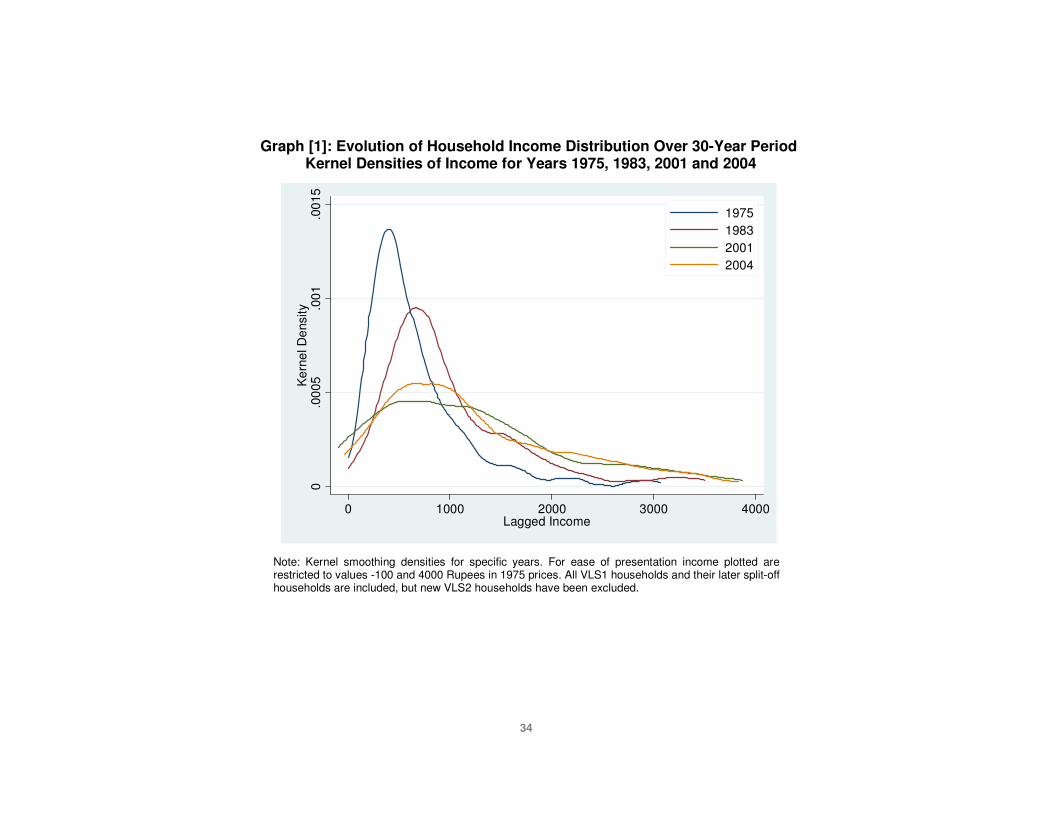
During the early panel, income shows a clear upward trend while income in the later
panel, VLS2, is substantially higher, most notably due to the 2001 and 2002 high
income years, a finding that coheres with the results of Badiani et al (2008). Graph [1]
provides an even more striking representation of the income increases benefiting the
households in the ICRISAT sample. The graph plots kernel densities of income for
individual years 1975, 1983, 2001 and 2004. We observe that not only has mean
income increased over this period, but the spread of the income distribution has also
grown dramatically. As we will argue later, the evidence presented in the paper goes
some way to explaining the observed expansion in income inequality.
Before moving to the discussion of the results of our parametric analysis, it is
instructive to plot the raw income data. The econometric model assumes that the
income generating process follows a polynomial function. Graph [2] uses locally
weighted (Lowess) methods to obtain a non-parametric estimate of income lagged
( 1, −tiy ) on current income ( tiy , ). The income patterns implied by the graph suggest
substantial convergence and few non-linearities in the income generating process. In
9 Additionally, given the structure of our data individuals belonging to the same household will have identical income values. The

16
the next section, we assess whether this remains an accurate description of the true
income generating process once issues of measurement error, income stochastic
patterns and unobserved heterogeneity have been addressed.
4.2 Regression results
As discussed in section 3 above, our econometric methodology estimates the
parameter of a polynomial function of lagged income in first-differenced form –
equation (2’) – using exogenous instruments. Tables [3] and [4] report IV GMM first
and second-stage estimates, for three alternative functions: linear, quadratic and cubic
polynomial. For each of these models, we estimate one specification with year
dummies and another without.
Columns (1) and (2) in Table [3] show that our instruments significantly affect changes
in income. When no year dummies are included, we find rainfall deviations significantly
increase household income. The significance of the signed square of the rainfall
deviations indicates a complex nonlinear relation between precipitation and income.
Similarly, the interaction effects between rainfall shocks and household characteristics
are significant and take signs as expected. We find that households operating larger
plots and households with fewer kids among their members appear to benefit (lose) the
most when rainfall is abundant (poor).
While estimates for interaction instruments remain largely unchanged when year
dummies are included, rainfall shocks lose their significance. When we include year
dummies, the income effect of rainfall shocks is exclusively identified by the variation in
village precipitation. Given that the pattern of rainfall in the Indian sub-continent is
mostly determined by the timing and profusion of the monsoon season, we would
expect rainfall shocks in a given year to be highly correlated across villages. It is
therefore not surprising to find rainfall shocks not to vary sufficiently across villages to
be identified beyond the annual effect. As other factors determining incomes may also
be common across villages, a specification with time dummies would seem more
appropriate. It is on this model specification that we focus throughout the paper.
clustering function will also yield standard errors corrected for the repeated nature of the data.

17
Evidence in columns (3) to (6) in Table [3] shows that both the signed square of rainfall
deviations as well as the interaction instruments are not only good predictors of the first
moment, but also of the second and third moments of income. Estimated coefficients
both take signs that make economic sense and are significant at standard levels of
confidence. However, when we test for their joint-significance we obtain relatively low
F-Statistic, 7.9, 8.1 and 7.1 for the first, second and third moments of income
respectively.
Even though instruments are correctly signed and are significant in explaining different
moments of the changes in lagged income, we cannot ignore inference problems
arising from ‘weak’ instruments. Indeed, the implied Cragg-Donald statistics suggest
that our IV GMM estimates might contain substantial finite-sample biases. We follow
two alternative strategies when addressing the issue of weak IVs. First, we estimate
the model with alternative estimators – such as LIML and Fuller estimators – which are
more robust to the presence of ‘weak’ IVs. Secondly, we re-estimate the quadratic
polynomial model with a parsimonious set of instruments, which improves the joint
explanatory power of the instruments and reduces the remaining bias in the
second-stage estimates. While we discuss in detail each of these strategies in the
appendix, we find reassuring that estimates from these alternative methods yield
results remarkably similar to the baseline model.
In Table [4] we present our main results. The table reports second-stage estimates for
the three different polynomial specifications. When including year dummies, we
uncover substantial annual shifts in income growth – most notably a drop in growth
between 2002 and 2003 and the subsequent rebound in 2004. This is consistent with
the incidence of failed monsoon rains that affected interior areas of Andrah Pradesh
and Maharashtra during the 2003, 2004 and 2005 Kharif season. Failing to control for
such large year-specific growth patterns – possibly related to aggregate shocks
affecting all villages – might hinder the identification of individual income dynamics.
Indeed, we find that the inclusion of year dummies dramatically improves the precision
in the estimates of the parameters of the polynomial.
As expected, when fitting a linear model we find a positive correlation between lagged
income and current income (see column 2). The coefficient is statistically significant

18
but modest in magnitude suggesting a relatively high degree of income mobility. In
columns (3) to (6) we report the results for the quadratic and cubic model
specifications.
Estimates for the quadratic model provide some striking results. First, we find that the
income generating process might not be linear in nature. When we include the
second-moment of lagged income we find it to be significant at the 5% level – see
column (4). Secondly, the point estimates for the first-moment of lagged income are
significant and very large in magnitude, suggesting convergence might be relatively
slow or even unachievable. Indeed, point estimates show that the income generating
process might follow a concave pattern, opening the possibility for the existence of
multiple equilibria.
When allowing for a third-moment in the income generating process (column 6), point
estimates change wildly and significance is lost. We attribute this to multicollinearity
and poor identification power of the IV GMM estimator. We show in the appendix that
alternative estimators – such as IV Fuller – perform better and yield estimates similar to
the quadratic model specification.10
As suggested earlier, ignoring attrition in a long panel such as ICRISAT might lead to
substantial biases in parameter estimates. Table [5] reproduces results for the IV GMM
estimates where we apply inverse probability weighting (IPW) methods. The weights
are computed as the inverse of the probability of attrition predicted by a vector of
individual and household characteristics measured at the beginning of the survey
period.11 Table [5] shows that point estimates are remarkably similar in magnitude to
our original estimates. In other words, while attrition in the ICRISAT sample is large
and almost certainly non-random, patterns of attrition appear to be relatively
orthogonal to income dynamics in the period of study. This is consistent with Badiani et
al (2008) where they find that correcting for attrition had relatively little impact on the
determinants of consumption growth over the same period. At the same time, we find
that significance of the estimated parameters is lost. This can be attributed to the loss
10The correlation coefficient between the second and third moment of lagged income in these regressions is very high, reaching 0.96 when estimating the model in column (6)). Other estimators seem to perform better under these conditions, the cubic models for the IPW IV GMM and IV Fuller estimates provide point estimates similar to the quadratic model parameters. See Appendix for Fuller estimates.

19
in efficiency from applying the IPW procedure (Wooldridge, 2002b) and is corroborated
by the increase in standard errors observed in Table [5] relative to the IV GMM
standard errors (see Table [4]).12
In the appendix, we discuss a number of further checks for robustness of the core
results. The finding that income dynamics in the ICRISAT villages appear to be driven
by a quadratic polynomial with pronounced concavity, remains robust to changing the
period of analysis, between the VLS1 and VLS2 panels, as well as applying alternative
estimation methods more robust to the presence of ‘weak’ IVs.
4.3 Multiple Equilibria and Household Heterogeneity
Showing that the current income follows a polynomial of lagged income with a concave
pattern does not constitute proof of the existence of multiple equilibria. For that we
need to show that the derivative of the resulting polynomial is larger than unity when
)( 1,, −= titi ygy – where the g-function represents the dynamic polynomial function – and
that this condition is met within the range of values of the income distribution.
Furthermore, in our model specification, household heterogeneity will shift the dynamic
patterns and therefore any potential multiple equilibria will be household specific (see
also Antman and McKenzie, 2005).
The easiest way to illustrate this is graphically. Graph [3] plots income simulations
based on the parameter estimates of the polynomial from the quadratic model
specification reported in Table [4].13 14
The results presented in Graph [3] are truly striking. First, when considering the
11 Attrition probit estimates are not reported, but results can be requested from the authors. 12 As a further robustness check of the impact of attrition on our estimates, we re-estimate our baseline model only with individuals present in every year of the panel. This reduces the sample size substantially – from 8279 to 3301 observations – as well as the external validity, but it ensures that the parameter estimates will accurately reflect, free from attrition bias, the income generating process for the sub-sample of non-attiring individuals. In spite of the substantial attrition and the reduction in sample size, we find that baseline results remain largely unchanged. If anything, parameters become larger in magnitude and more precisely estimated. Results not reported in the paper. 13 We report in the Appendix the full set of simulations based on all six of the specifications estimated in Table [4]. After recovering the household fixed effects implied by the model estimates, we plot the dynamic simulations for different percentiles of the fixed effects distribution. Specifically Graph [3] reports the simulated dynamic path for the 10th, 50th and 90th percentiles of the individual fixed effects. 14 As one would expect, robustness checks on simulated dynamics provide a similar results as for model estimates. We find that using ‘weak’ IV robust estimators as well as attrition correction methods, does not change the simulated dynamics. See Graph [A2] in the Appendix.
20
dynamic path for the median household, we find two equilibria in the range of
reasonable values of income: namely a high stable equilibrium, and a low unstable
saddle point. The high stable equilibrium is approximately 1900 Rupees per adult per
year in 1976 prices, approximately 210 US dollars at the exchange rates at that time.
The lower unstable equilibrium is about Rp 500 or 55 US dollars. The derived dynamic
path implies that households with fixed effect values close to the median will face a
divergence point or threshold whereby the dynamic paths separate. Namely,
household lying above the saddle point will converge over time towards the high
equilibrium while households below the saddle point will inevitably suffer further losses
in their future income. Lying below the threshold or being pushed over it by shocks
such as rainfall would appear to put households on a path towards ‘perdition’.
A second aspect to note from Graph [3] is that not all households are exposed to the
risk of destitution. Households with sufficiently high individual fixed effects, as
represented by the top decile in Graph [3], have a single dynamic equilibrium. For this
type of households, we expect their income levels to converge – although the rate of
convergence suggested by the concave polynomial would appear to be very slow,
even for relatively high values of lagged income. Furthermore, the existence of a single
equilibrium for this group of households cannot be understated. Even when faced with
large shocks, these households would appear to face little risk of being put on a path of
structural divergence. It is as if their livelihood faces no vulnerability: even if they
occasionally have low incomes, they won’t get stuck there permanently.
Thirdly, among households with low fixed effects, we find that the dynamic path also
appears to experience multiple equilibria. However, for this group vulnerability does
have a qualitatively different meaning than for other households. For low levels of fixed
effect income, the stable equilibrium and the divergence threshold are close to each
other. In other words, for households that have already reached their steady state
equilibrium, a relatively small shock could push them over the divergence threshold.
Furthermore, it should be noted that the lower the fixed effects, the higher lies the
saddle point. In other words, households with low fixed effects could be set on a
structural divergence path even though they might have values of current income
higher than households with higher fixed effects that are on a convergence path
towards their high stable equilibrium.

21
Two further points are worth noting. Analysing the median household dynamic path we
see that the threshold for this group lays on a relatively low value of income. It is
therefore plausible that most households might have current income above the
threshold, resulting in a relatively low risk of structural destitution. If this applies to the
median, it is possible that the risk of being set on a divergence path is only real for a
relatively small sub-sample of households. However, Graph [3] provides some
evidence against this possibility. Comparing the median versus the bottom decile
households’ curves, we see that there is only a small vertical distance between the two.
In other words, half of our sample faces a dynamic threshold that lays between 500
and 1200 Rupees – the unstable equilibrium for the bottom decile.
Additionally, although clear from the graph, it is instructive to recognise the fact that
households on a convergence path will ultimatively converge to their own steady state
equilibrium. Their eventual steady state income level – and arguably their level of
long-term welfare – will therefore depend on their own individual fixed effects. This
feature combined with the high inequality in the individual fixed effects in the top of the
distribution – as represented by the large vertical distance between the median and the
top decile of fixed effects – predict substantial structural growth for this group of
individuals. This prediction would appear to be consistent with the dramatic increases
observed in income inequality over the period of analysis depicted in Graph [1]
4.4 Unpacking Individual Fixed Effects
The importance of the individual fixed effects can hardly be overstated. Not only do
they determine the steady state income households will eventually reach, but
individuals with fixed effects approximately below the median are faced with the real
possibility of suffering a shock that might put them on a dynamic path towards
destitution. It is with this in mind that we now move towards understanding what lies
behind these fixed effects.
To retrieve some idea of the correlates of income fixed effects, we regress them on a
set of starting period household characteristics as measured at the beginning of our
panel in 1975. Columns (1) and (2) in Table [6] report the correlates of individual fixed
effects from the quadratic models (3) and (4) in Table [4]. These columns include

22
time-invariant household characteristics only as determinants of household fixed
effects, while columns (3) and (4) include ‘land area owned’ and ‘value of household
assets’ as additional time-varying correlates.
We find results in Table [4] are robust across all polynomial models. For our preferred
model, the quadratic polynomial with year dummies, we find that beyond village
dummies, education of the household head appears to be significantly correlated with
fixed effect income. When we add land ownership and value of assets to education, we
find all three to be strongly correlated with the fixed effects. Despite their geographic
proximity, these villages have substantial heterogeneity in soil and other
characteristics (Walker and Ryan, 1990). Correspondingly, individuals in different
villages have different income trajectories: compared to village Aurepalle in the state of
Andhra Pradesh, the default category, villages Shirapur, Kalman and Kinkheda in the
state of Maharashtra have substantially lower fixed effects.
We interpret these results as suggestive that while changes in India over the past 30
years have increasingly created opportunities for substantial welfare improvements,
not all households have been in the position to benefit. Human capital and physical
assets appear crucial in ensuring that households are well enough equipped to take up
the new opportunities.
5 Conclusions
A variety of theories suggest why a person who becomes poor at any time will remain
poor indefinitely. Most such theories focus on a technology with increasing returns to
scale which arises from a particular social mechanism – nutrition, education, fixed
costs to entering a business, or another. The ideas of poverty traps that arise from
these theories constitute a central theory of development economics at both the micro
and macro levels. But these theories have received extremely little empirical support,
possibly due to econometric pitfalls in the methods underlying the relevant empirical
studies, as Dasgupta (1997) argues occurs for tests of the nutrition-efficiency wage
theory, or possibly because no poverty trap in fact exists.
The large number of people in extreme penury constitutes only one reason
23
underpinning the importance of understanding whether and why the destitute escape
poverty. The presence of poverty traps would also implies a startling policy conclusion:
a small transfer to a poor individual or household could change that person from low- to
high-level equilibrium and permanently remove a person from poverty.
Since most existing theories of poverty traps assume some form of fixed investment
cost, or increasing returns to assets or income, we examine whether income dynamics
give evidence of increasing returns. A variety of econometric problems arise in this
analysis: lagged income is inherently endogenous in a dynamic panel model;
measurement error in income will cause OLS or GMM estimates to understate
income's persistence; individual heterogeneity may disguise the fact that some
individuals face a poverty trap even though the average individual does not; and short
panel duration may give inadequate time to observe sufficient movement in income.
The bivariate kernel regressions or Arellano-Bond methods that existing papers use
address some but not all of these pitfall. We apply IV GMM methods in a dynamic
income equation that addresses issues of measurement error and endogeneity of
lagged income, while allowing household heterogeneity in income steady state. Unlike
similar studies (Jalan and Ravallion, 2003 and Lokshin and Ravallion, 2004), we use
exogenous instruments in exploiting deviations in annual precipitation to explain future
income. Indeed, first-stage estimates reveal rainfall deviations to be a strong predictor
of year-on-year changes. In particular, we interact rainfall with household land
operated and household composition variables to obtain valid and relatively strong
instruments for a polynomial function of contemporaneous income.
Our analysis shows that income generating dynamics in rural India follow a quadratic
polynomial function with pronounced concavity. We find these results to be robust to
changes in the period of analysis and corrections for non-random attrition. Further,
parameter estimates obtained applying alternative estimation methods more robust to
the presence of ‘weak’ IVs, remain consistent with our original results.
A recent study applying non-parametric methods to the same dataset as ours, reports
income mobility to be static but provides no evidence of the existence of multple
equilibria (Nashold, 2009). When allowing for individual heterogeneity and using

24
exogenous instruments to address income endogeneity, our analysis provides a
different conclusion. Income simulations based on the estimated parameters suggest
the presence of two distinct equilibria: a stable high-income equilibrium and a low-level
unstable saddle point. While households with sufficiently high fixed effect income
follow the high-equilibrium dynamic path, almost half of our sample has too low an
income steady state to overcome the dynamic point of divergence. Analysis of income
fixed effects shows that schooling and other assets at the beginning of the sample
period are linked to high levels of steady state income.
We interpret our results as suggesting that changes in India over the past 30 years
increasingly provide opportunities for substantial welfare improvements, but not all
households are well place to benefit. Education appears crucial in ensuring these
opportunities are being taken. Those with higher assets have an income process with a
much lower low-level unstable equilbrium than those with fewer assets: the latter’s
lives are far more precarious and even at higher income levels they risk sliding down
dramatically. For some with high assets, this low unstable equilibrium would
correspond to large negative current income positions. While in an agricultural setting
occassional negative incomes are possible (and indeed observed in the data), it
suggests that only a rather high and almost improbable income draws they would face
such outcomes.
25
Appendix
A.1 Estimation with Weak Instruments
As discussed in section 2, consistent IV GMM estimates require two instrumental
variable conditions to hold, the ‘validity’ condition and the ‘strong IV’ condition. The
validity condition states that the set of instruments should not be correlated with any
unobserved determinant of income. The exogenous nature of the rainfall shocks and
its potential heterogeneous effects, suggest that our set of instruments is unlikely to be
invalid. Indeed, Hansen J Overidentification statistic reported in Table [4] indicates that
we cannot reject the null hypothesis that all excluded instruments are exogenous.
However, Cragg-Donald F-statistics related to Table [4] suggest that our set of
instruments might not be sufficiently strong. Although our excluded instruments are
good predictors of individual moments of lagged income, the Cragg-Donald statistics
test the null that the set of excluded instruments is jointly sufficiently strongly correlated
with the set of endogenous variables. We find that in spite of first-stage F-Statistics of
7.90, 8.10 and 7.10 for the three-moments of changes in lagged income, the
Kleibergen-Paap rank corrected Cragg-Donald statistics amounts to values of 3.5
and .0.0028 for the quadratic and cubic models with year dummies, respectively.
When compared with Stock-Yogo critical values, these Cragg-Donald statistics
suggest the presence of ‘weak’ instruments resulting in IV GMM estimates containing
absolute biases approximately exceeding 30%.
Such magnitude of bias casts doubts on the reliability of the results presented earlier.
Here we present two alternative approaches designed to provide further evidence of
the robustness of our earlier results. First, we apply alternative estimators that are
more robust to ‘weak’ instruments. We use LIML and Fuller estimators to obtain
alternative point estimates for our main TSLS results. Secondly, in a world of weak IVs,
the size of the resulting bias is understood to increase with the number of instruments
(Stock and Yogo, 2005). As a robustness checks we re-estimate our quadratic model,
using only the interaction effects of the rainfall shocks. While removing the rainfall
shock itself from the instrument set might reduce the bias, this comes at little cost, as

26
rainfall shock themselves are not significant when the model is estimated with year
dummies.
Table [A1] in the Appendix reproduces Table [4] for the alternative LIML and Fuller
estimators. Comparing these results with the IV GMM estimates, we find that, both
point estimates and significance remain robust to estimation by LIML and Fuller.15
Although still suspect of suffering from weak IV bias, we draw some comfort from the
fact that these alternative estimators provide point estimates consistent with the IV
GMM estimates.
Additionally, Table [A2] reports results for our ‘parsimonious IV’ estimates of the
quadratic model with year dummies. Using only the rainfall shocks interacted with land
area and with the number of kids in the household, we improve the strength of our
instrument. First-stage F-Stats increase to 10.10 and 9.70 for first and second
moments respectively, and the Cragg-Donald statistic reaches a value of 4.22.
Although the latter is not sufficiently high for weak IVs to be ruled out, the revised
estimates would be expected to contain a smaller bias. Specifically, Stock-Yogo (2005)
critical values for the IV GMM/LIML model suggest an absolute bias less than 20%.
Results reported in Table [A2] are broadly consistent with our earlier results. It is also
interesting to note that relative to LIML and Fuller estimates with three excluded
instruments in Table [A1] as well as to IV GMM estimates in Table [4], points estimates
in the parsimonious IV model increase in magnitude for both the first and second
moment. We interpret this change as an indication that the remaining ‘weak’ IV bias
might be biasing downward the estimated parameters. In other words, the estimated
dynamic patterns might be understating the degree of persistence and concavity of the
true income generating process. Table [4] also shows that our ‘parsimonious IV’ results
are also robust to correcting for attrition in observables.
The weak IV bias could also have implications to the dynamic simulations. Graph [A2]
in the Appendix, reproduces the simulation dynamics for the Fuller regressions using
the ‘parsimonious IV’ set reported in Table [A2]. We find that the estimated dynamics
15 Note that the LIML estimation methods is identical to the IV GMM procedure when the model is just identified, which is the case in our analysis when we estimate the cubic polynomial model.

27
remain consistent with our original results. This is also the case when we correction for
attrition in observables.
It should be noted that it is unclear whether the Cragg-Donald statistic is the
appropriate diagnostic in our case. Our model specification is a particular case of a
system of equations ‘nonlinear in the endogenous variables’ – to use the terminology in
Wooldridge (2002b). By virtue of the second and third moments of lagged income
being nonlinear functions of lagged income, the identifying conditions (rank and order)
for the system are the same as in the case of the simple linear lagged income case
(Fisher, 1965). In effect, any additional nonlinear term arrives with its own instruments
– namely the first and higher moments of the instruments used in predicting the linear
endogenous variable. For the assessment of the rank condition, Fisher (1965)
proposes to treat the nonlinear terms as independent additional variables but should
be excluded from the rank condition tests.
The Cragg-Donald F-Statistic in its original form and the Kleibergen-Paap rank
corrected version, treat each endogenous variable as an independent equation; an
assumption that would appear inappropriate in our case. Indeed, the performance of
the Cragg-Donald statistic in our ‘parsimonious IV’ model casts further doubts on the
validity of the test. While individually the first and second moments appear to be strong
instruments following the Staiger and Stock rule of thumb – with F-Statistics of 10.10
and 9.70 respectively – the Cragg-Donald statistic yields a value (4.22) that would
nevertheless predict a bias close to 20%.
In the case of a system of equations nonlinear in endogenous variables, Wooldridge
(2002b) suggests an alternative estimation approach: instead of treating the nonlinear
terms as independent variables, the nonlinear relation between the different moments
can be explicitly exploited. Wooldridge proposes a procedure that use 21)ˆ( −ty as a
single instrument for 21−ty , where the former is the square of the predicted first-moment
of lagged income using the set of excluded instruments (p. 237, Wooldridge, 2002b).
While more parsimonious, when we apply this alternative estimation methodology to
our quadratic polynomial model, we find that – with an F-Statistic of 1.66 – the
predictive power of 21)ˆ( −ty on 2
1−ty is in fact lower than the predictive power of the
28
excluded instruments. If we nevertheless estimate the parameters of the quadratic
polynomial following Wooldridge (2002b) we obtain estimates 2
11 )(*000127.0*51.0 −− −= ttt yyy . These estimates suggest a concave dynamic
function with a single stable equilibrium, but low speed of convergence.
A.2 Parameter Stability and Panel Structure
Our model specification assumes that a single set of polynomial parameter values
underlie the income generating process. However, considering the 15-year gap
between VLS1 and VLS2, it is plausible that income dynamics have dramatically
changed during that time. We address this issue by testing the parameter stability of
the income polynomial function across the two panel periods. Table [A3] reports results
from estimating the quadratic model specification for the VLS1 and VLS2 panel
samples separately. We find that VLS1 estimates have strong IVs – according to the
Cragg-Donald test with the Kleibergen-Paap rank correction – and report parameter
estimates broadly consistent with the full panel.
On the other hand, estimates for the VLS2 panel indicate the presence of severely
weak instruments. Point estimates are also very imprecisely estimated. Both of these
findings should not be surprising as we effectively estimate our differencing model
using a two-period panel (2003 and 2004) only. Moreover, the dramatic income
increases experienced during 2001 and 2002 – see Table [2] –, imply that the VLS2
sample might be a particularly noisy period in which to estimate income dynamics with
a short time component. It is therefore especially encouraging to nevertheless find that
point estimates are remarkably similar to estimates for the VLS1 sample only.
Accordingly dynamic simulations presented in Graph [A3] show very similar patterns
between the two periods. We note that while the point of divergence appears stable
between the periods, the higher stable equilibrium is substantially higher in the later
panel. At the same time, estimated fixed effects in VLS2 appear to have a higher
spread. Each of these findings is consistent with the rise in income variance shown in
Graph [1] and suggest that the increased opportunities that modern India has to offer
appear to be benefiting only a fraction of households.
29
More formally we test for the parameter stability between the two periods applying a
pooling test or Chow test. We augment the quadratic dynamic model as characterised
in equation (1) with interaction effects for the VLS1 and VLS2 periods with each of the
dynamic terms. The Chow test analysis the null hypothesis that the dynamic
parameters are identical between the two periods. Unable to appropriately estimate
the augmented model by two-stage least squares – faced with impossible task of
instrumenting six endogenous variables –, we apply the test instead to the OLS model.
The results of the Chow test are in line with earlier evidence; we find that the stability of
the quadratic polynomial parameters estimated by OLS can not be rejected.16
16 Results of the parameter stability test can be requested from the authors.
30
References
Adato, Michelle, Michael. Carter, and Julian May. Exploring Poverty Traps and Social Exclusion in South Africa Using Qualitative and Quantitative Data. Journal of Development Studies 42(2):26–247, 2006 Anderson, T.W. and Cheng Hsiao. Formulation and Estimation of Dynamic Models Using Panel Data. Journal of Econometrics, 18(1):47-82, 1982.
Antman, Francesca and David McKenzie. Poverty traps and Nonlinear Income Dynamics with Measurement Error and Individual Heterogeneity. Journal of Development Studies 43 (6) 1057-1083, 2007. Arellano, Manuel and Stephen Bond. Some Tests of Specification for Panel Data: Monte Carlo Evidence and an Application to Employment Equations. Review of Economic Studies, 48(2):277-297, 1991. Azariadis, C. and J.Stachurski. Poverty Traps. in P.Aghion and S. Durlauf (eds.) Handbook of Economic Growth, vol.1, no.1, Elsevier North Holland, 2005.
Badiani, Reena, Stefan Dercon, Pramila Krishnan and K.P.C. Rao. Changes in Living Standards in Villages in India 1975-2004: Revisiting the ICRISAT village level studies. CPRC Working Paper Series, no. 85, 2008. Banerjee, Abhijit and Andrew Newman. Occupational Choice and the Process of Development. Journal of Political Economy, 101(2):274-298, 1993. Barrett, C.B., P.P. Marenya, J.G. McPeak, B. Minten, F. Murithi, W. Oluoch-Kosura, F. Place, J.C. Randrianarisoa, J. Rasambainarivo, and J. Wangila. Welfare Dynamics in Rural Kenya and Madagascar. Journal of Development Studies 42:248–277, 2006
Bliss, Christopher J. and Nicholas H. Stern. Palanpur: The economy of an Indian village. Oxford University Press, Oxford, 1982.
Blundell, Richard and Stephen Bond and Frank Windmeijer. Estimation in dynamic panel data models: improving on the performance of the standard GMM estimators. 2000.
Bond, Stephen R. Dynamic panel data models: a guide to micro data methods and practice. Portuguese Economic Journal, 1(2):141-162, 2002.
Bound, John and David A. Jaeger and Regina M. Baker. Problems with Instrumental Variables Estimation When the Correlation Between the Instruments and the Endogenous Explanatory Variable is Weak. Journal of the American Statistical Association, 90(430):443-450, 1995.
Bound, John and Alan B. Krueger. The Extent of Measurement Error in Longitudinal Earnings Data: Do Two Wrongs Make a Right?. Journal of Labor Economics,

31
9(1):1-24, 1991. Carter, Michael and Chris Barrett. The economics of poverty traps and persistent poverty: An asset based approach. Journal of Development Studies, 42, 178–199, 2006
Chen, Shaohua and Martin Ravallion. “The Developing World Is Poorer Than We Thought, But No Less Successful in the Fight against Poverty”, Policy Research Working Paper 4703, The World Bank. 2008.
Dasgupta, Partha and Debraj Ray. Inequality as a Determinant of Malnutrition and Unemployment: Theory. The Economic Journal, 96(384), 1986. Dasgupta, Partha, “An Enquiry into Well-Being and Destitution”, Oxford University Press, 1993.
Dercon, Stefan and Joseph Shapiro. “Moving On, Staying Behind, Getting Lost: Lessons on poverty mobility from longitudinal data”, chapter in Deepa Narayan and Patti Petesch, Moving out of Poverty, World Bank 2007.
Fan, Jianqing. Design-adaptive Nonparametric Regression. Journal of the American Statistical Association, 87(420), 1992. Fisher, Franklin M. Identifiability Criteria in Nonlinear Systems: A Futher Note. Econometrica, 33, 197-205, 1965
Fitzgerald, John and Peter Gottschalk and Robert Moffitt. An Analysis of Sample Attrition in Panel Data: The Michigan Panel Study of Income Dynamics. Journal of Human Resources, 33(2):251-299, 1998. Galor, Oded and Joseph Zeira. Income Distribution and Macroeconomics. Review of Economic Studies, 60(1):35-52, 1993.
Heckman, James J. Formulation and Estimation of Dynamic Models Using Panel Data. Econometrica, 47(1):153-162, 1979.
Jacoby, Hanan and Emmanuel Skoufias. Estimating the Return to Schooling: Progress on Some Persisitent Econometric Problems. Review of Economic Studies, 64, 1997.
Jalan, Jyotsna and Martin Ravallion. Insurance Against Poverty, chapter Household Income Dynamics in Rural China. Oxford University Press, 2003.
Lokshin, Michael and Martin Ravallion. Household Income Dynamics in Two Transition Economies. Studies in Nonlinear Dynamics & Econometrics, 8(3), 2004.
McKenzie, David and C Woodruff. Do Entry Costs Provide an Empirical Basis for Poverty Traps? Evidence from Mexican Microenterprises Economic Development and Cultural Change, Vol. 55, pages 3-42, 2006.

32
Mookherjee, Dilip and Debraj Ray. Contractual Structure and Wealth Accumulation. American Economic Review, 92(4):818-849, 2002. Mookherjee, Dilip and Debraj Ray. Aspirations, Segregation and Occupational Choice. Journal of the European Economic Association, Vol. 8, No. 1, Pages 139-168, 2010 Munshi, Kaivan and Mark Rosenzweig. Why is Mobility in India so Low? Social Insurance, Inequality, and Growth. NBER Working Papers 14850, 2009,
Murray, Michael. Avoiding Invalid Instruments and Coping with Weak Instruments. Journal of Economic Perspectives. American Economic Association, vol. 20(4), pages 111-132, 2006a. Murray, Michael. The Bad, the Weak, and the Ugly: Avoiding the Pitfalls of Instrumental Variables Estimation, 2006b. Available at SSRN: http://ssrn.com/abstract=843185. Naschold, F. Poor stays poor - Household Asset Poverty Traps in Rural Semi-arid India. Mimeo. 2009. Nickell, Stephen. Biases in Dynamic Models with Fixed Effects. Econometrica, 49(6):1417-1426, 1981. Quisumbing, Agnes and Bob Baulch. Assets and Poverty Traps in Rural Bangladesh. IFPRI Working Papers, July 2009, No. 143. 2009 Ray, Debraj. Aspirations, Poverty, and Economic Change in Understanding Poverty, Oxford University Press, 2006 Rosenzweig, Mark R. Labour markets in low-income countries in Handbook of Development Economics . North-Holland, Amsterdam, 1988.
Stock, James H. and Jonathan H. Wright and Motohiro Yogo. A Survey of Weak Instruments and Weak Identification in Generalized Method of Moments. Journal of Business and Economic Statistics, 20(4):518-529, 2002. Stock, J. H., and M. Yogo. Testing for Weak Instruments in Linear IV Regression. In Identification and Inference for Econometric Models: Essays in Honor of Thomas Rothenberg, ed. D.W. Andrews and J. H. Stock, 80–108, 2005. Swamy, Anand V. A simple test of the nutrition-based efficiency wage model. Journal of Development Economics, 53:85-98, 1997.
Walker, Thomas S. and James G. Ryan. Village and Household Economies in India's Semi-Arid Tropics. Johns Hopkins Press, Baltimore, 1990.
Wooldridge, Jeffrey M. Inverse probability weighted M-estimators for sample selection, attrition, and stratification. Institute for Fiscal Studies Working Paper CWP11/02, 2002a.

33
Wooldridge, Jeffrey M. Econometric Analysis of Cross Section and Panel Data. MIT Press, Cambridge, MA, 2002b.
34
Graph [1]: Evolution of Household Income Distribution Over 30-Year Period Kernel Densities of Income for Years 1975, 1983, 2001 and 2004
0.0
005
.001
.001
5K
erne
l Den
sity
0 1000 2000 3000 4000Lagged Income
1975198320012004
Note: Kernel smoothing densities for specific years. For ease of presentation income plotted are restricted to values -100 and 4000 Rupees in 1975 prices. All VLS1 households and their later split-off households are included, but new VLS2 households have been excluded.

35
Graph [2]: Bivariate Lowess Estimates of Current Household Income on Lagged Household Income, and Kernel Densities of Lagged Income
0.0
002
.000
4.0
006
.000
8.0
01D
ensi
ty -
Lagg
ed In
com
e
010
0020
0030
0040
00P
redi
cted
Cur
rent
Inco
me
0 1000 2000 3000 4000Lagged Income
Lowess Kernel Smoothing - Current Income45 Degree LineKernel Density - Lagged Income
Note: 45-degree line indicates locus where current income equals lagged income. Data used for the graphs is restricted to the years used in the parametric analysis, namely 1977-1983, and 2003-2004. For ease of presentation income plotted are restricted to values -100 and 4000 Rupees in 1975 prices. Parametric analysis in the paper uses all income values. All VLS1 households and their later split-off households are included, but new VLS2 households have been excluded.
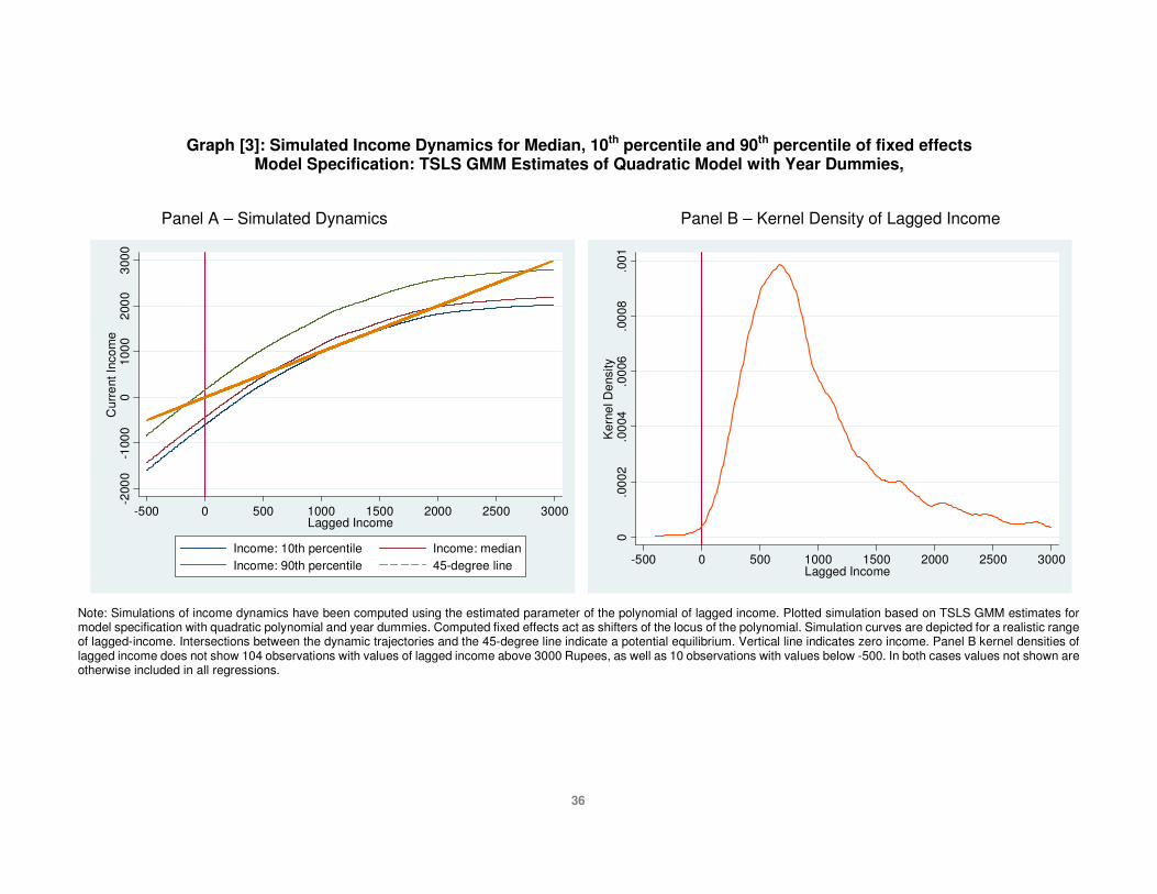
36
Graph [3]: Simulated Income Dynamics for Median, 10th percentile and 90th percentile of fixed effects Model Specification: TSLS GMM Estimates of Quadratic Model with Year Dummies,
Panel A – Simulated Dynamics Panel B – Kernel Density of Lagged Income
-200
0-1
000
010
0020
0030
00C
urre
nt In
com
e
-500 0 500 1000 1500 2000 2500 3000Lagged Income
Income: 10th percentile Income: medianIncome: 90th percentile 45-degree line
0.0
002
.000
4.0
006
.000
8.0
01K
erne
l Den
sity
-500 0 500 1000 1500 2000 2500 3000Lagged Income
Note: Simulations of income dynamics have been computed using the estimated parameter of the polynomial of lagged income. Plotted simulation based on TSLS GMM estimates for model specification with quadratic polynomial and year dummies. Computed fixed effects act as shifters of the locus of the polynomial. Simulation curves are depicted for a realistic range of lagged-income. Intersections between the dynamic trajectories and the 45-degree line indicate a potential equilibrium. Vertical line indicates zero income. Panel B kernel densities of lagged income does not show 104 observations with values of lagged income above 3000 Rupees, as well as 10 observations with values below -500. In both cases values not shown are otherwise included in all regressions.

37
Graph [4]: Attrition Correction – Simulated Income Dynamics for Median, 10th percentile and 90th percentile of fixed effects Model Specification: TSLS GMM Estimates of Quadratic Model with Year Dummies, with and without Attrition Correction
Panel A – TSLS GMM Panel B – TSLS GMM with IPW Attrition Correction
-200
0-1
000
010
0020
0030
00C
urre
nt In
com
e
-500 0 500 1000 1500 2000 2500 3000Lagged Income
Income: 10th percentile Income: medianIncome: 90th percentile 45-degree line
-200
0-1
000
010
0020
0030
00C
urre
nt In
com
e
-500 0 500 1000 1500 2000 2500 3000Lagged Income
Income: 10th percentile Income: medianIncome: 90th percentile 45-degree line
Note: Simulations of income dynamics have been computed using the estimated parameter of the polynomial of lagged income. Plotted simulations based on IV GMM estimates for model specification with quadratic polynomial and year dummies (Panel A) as well as with Inverse Probability Weighting (IPW) attrition correction (Panel B). Computed fixed effects act as shifters of the locus of polynomial. Simulation curves are depicted for a realistic range of lagged-income. Intersections between the dynamic trajectories and the 45-degree line indicate a potential equilibrium. Vertical line indicates zero income.
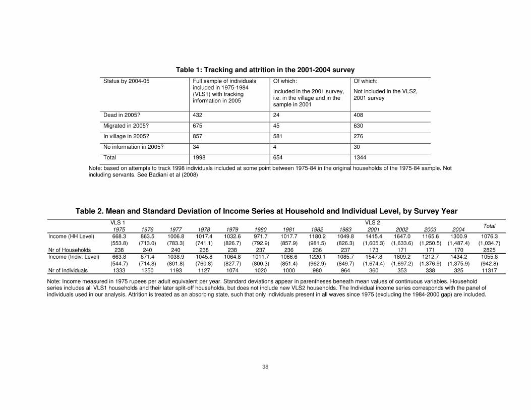
38
Table 1: Tracking and attrition in the 2001-2004 survey Status by 2004-05 Full sample of individuals
included in 1975-1984 (VLS1) with tracking information in 2005
Of which:
Included in the 2001 survey, i.e. in the village and in the sample in 2001
Of which:
Not included in the VLS2, 2001 survey
Dead in 2005? 432 24 408
Migrated in 2005? 675 45 630
In village in 2005? 857 581 276
No information in 2005? 34 4 30
Total 1998 654 1344
Note: based on attempts to track 1998 individuals included at some point between 1975-84 in the original households of the 1975-84 sample. Not including servants. See Badiani et al (2008)
Table 2. Mean and Standard Deviation of Income Series at Household and Individual Level, by Survey Year
1975 1976 1977 1978 1979 1980 1981 1982 1983 2001 2002 2003 2004Income (HH Level) 668.3 863.5 1006.8 1017.4 1032.6 971.7 1017.7 1180.2 1049.8 1415.4 1647.0 1165.6 1300.9 1076.3
(553.8) (713.0) (783.3) (741.1) (826.7) (792.9) (857.9) (981.5) (826.3) (1,605.3) (1,633.6) (1,250.5) (1,487.4) (1,034.7)Nr of Households 238 240 240 238 238 237 236 236 237 173 171 171 170 2825Income (Indiv. Level) 663.8 871.4 1038.9 1045.8 1064.8 1011.7 1066.6 1220.1 1085.7 1547.8 1809.2 1212.7 1434.2 1055.8
(544.7) (714.8) (801.8) (760.8) (827.7) (800.3) (851.4) (962.9) (849.7) (1,674.4) (1,697.2) (1,376.9) (1,375.9) (942.8)Nr of Individuals 1333 1250 1193 1127 1074 1020 1000 980 964 360 353 338 325 11317
VLS 1 VLS 2 Total
Note: Income measured in 1975 rupees per adult equivalent per year. Standard deviations appear in parentheses beneath mean values of continuous variables. Household series includes all VLS1 households and their later split-off households, but does not include new VLS2 households. The Individual income series corresponds with the panel of individuals used in our analysis. Attrition is treated as an absorbing state, such that only individuals present in all waves since 1975 (excluding the 1984-2000 gap) are included.

39
Table 3. First Stage Results – Impact of Rainfall on Lagged Income
Dependent variable: �Y t-1 �Y t-1 �Y t-12
�Y t-12
�Y t-13
�Y t-13
(1) (2) (3) (4) (5) (6)Square Rainfall shock, t-1 0.0007** 0.0004 3.5253** 2.8780* 1.9e+04* 1.4e+04*
(0.000) (0.000) (1.71E+00) (1.51E+00) (1.20E+04) (7.70E+03)Rainfall shock * land operated (ha), t-1 28.7496*** 13.5687 1.4e+05*** 1.0e+05* 6.0e+08** 5.2e+08*
(9.486) (10.479) (5.00E+04) (5.40E+04) (2.50E+08) (2.70E+08)Rainfall shock * children 0-8 in HH, t-1 -9.1588** -27.8874*** -6.5e+04*** -1.1e+05*** -3.7e+08*** -4.8e+08***
(4.529) (6.485) (2.00E+04) (2.40E+04) (1.20E+08) (1.10E+08)�Year: 1977 228.1362*** 5.9e+05*** 1.9e+09***
(35.671) (1.40E+05) (6.00E+08)�Year: 1978 194.7497*** 5.0e+05** 1.30E+09
(51.615) (2.30E+05) (9.80E+08)�Year: 1979 14.1897 -150,000.00 -9.60E+08
(41.736) (1.70E+05) (7.20E+08)�Year: 1980 42.9072 160,000.00 8.90E+08
(40.541) (1.90E+05) (9.40E+08)�Year: 1981 -49.6454 -170,000.00 -900000000
(50.153) (2.20E+05) (1.10E+09)�Year: 1982 62.6628 99,000.00 5.60E+08
(52.514) (2.10E+05) (9.90E+08)�Year: 1983 195.2823*** 7.0e+05*** 2.9e+09***
(36.451) (1.80E+05) (9.90E+08)�Year: 2003 342.6323** 1,300,000.00 8.60E+09
(145.482) (9.30E+05) (7.20E+09)�Year: 2004 -7.7e+02*** -3.3e+06*** -1.9e+10*
(161.081) (1.30E+06) (1.00E+10)Observations 8279 8279 8279 8279 8279 8279R-squared 0.0071 0.0776 0.0050 0.0388 0.0024 0.0224F Test for joint significance of IV 6.3751 7.9327 4.8832 8.0919 3.8767 7.0878
Note: Standard errors robust to heteroskedasticity and ‘original’ household-level clustering appear in parentheses. Income measured as real Rupees per adult equivalent. ‘Rainfall shock’ measured as the ratio between Kharif precipitation (rainy season) and the Kharif historic precipitation as observed across all waves of the panel. ‘Rainfall shock’ is interacted with the size of land operated in hectares as well as the number of children aged 0-8 in the household. Variable ‘Square Rainfall shock’ is the ‘signed’ square of the Kharif precipitation difference in a wave and the historic mean.
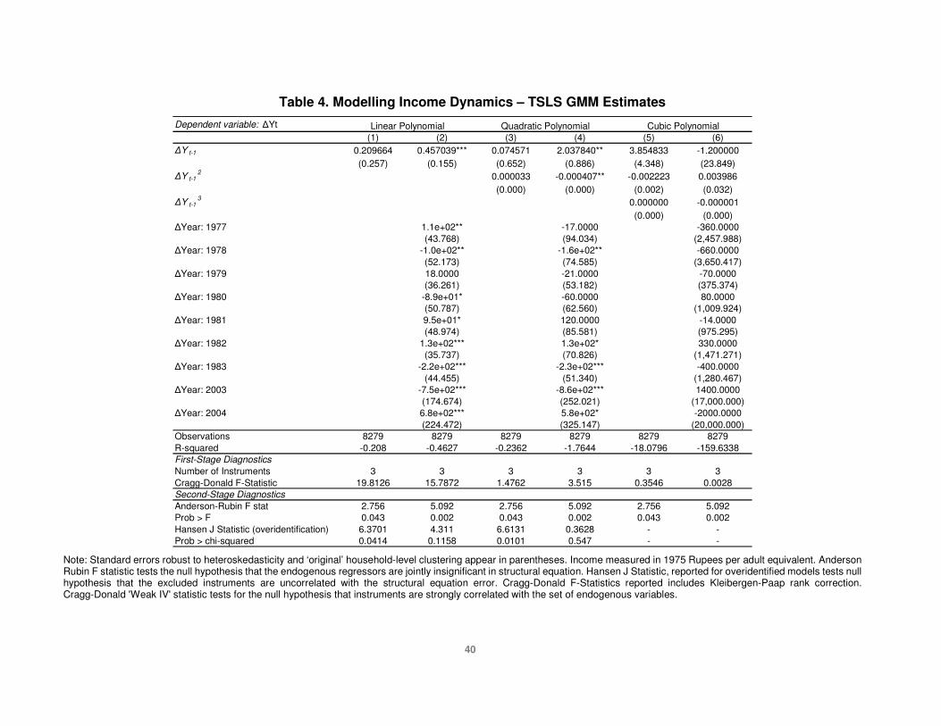
40
Table 4. Modelling Income Dynamics – TSLS GMM Estimates
Dependent variable: �Yt(1) (2) (3) (4) (5) (6)
�Y t-1 0.209664 0.457039*** 0.074571 2.037840** 3.854833 -1.200000(0.257) (0.155) (0.652) (0.886) (4.348) (23.849)
�Y t-12 0.000033 -0.000407** -0.002223 0.003986
(0.000) (0.000) (0.002) (0.032)�Y t-1
3 0.000000 -0.000001(0.000) (0.000)
�Year: 1977 1.1e+02** -17.0000 -360.0000(43.768) (94.034) (2,457.988)
�Year: 1978 -1.0e+02** -1.6e+02** -660.0000(52.173) (74.585) (3,650.417)
�Year: 1979 18.0000 -21.0000 -70.0000(36.261) (53.182) (375.374)
�Year: 1980 -8.9e+01* -60.0000 80.0000(50.787) (62.560) (1,009.924)
�Year: 1981 9.5e+01* 120.0000 -14.0000(48.974) (85.581) (975.295)
�Year: 1982 1.3e+02*** 1.3e+02* 330.0000(35.737) (70.826) (1,471.271)
�Year: 1983 -2.2e+02*** -2.3e+02*** -400.0000(44.455) (51.340) (1,280.467)
�Year: 2003 -7.5e+02*** -8.6e+02*** 1400.0000(174.674) (252.021) (17,000.000)
�Year: 2004 6.8e+02*** 5.8e+02* -2000.0000(224.472) (325.147) (20,000.000)
Observations 8279 8279 8279 8279 8279 8279R-squared -0.208 -0.4627 -0.2362 -1.7644 -18.0796 -159.6338First-Stage DiagnosticsNumber of Instruments 3 3 3 3 3 3Cragg-Donald F-Statistic 19.8126 15.7872 1.4762 3.515 0.3546 0.0028Second-Stage DiagnosticsAnderson-Rubin F stat 2.756 5.092 2.756 5.092 2.756 5.092Prob > F 0.043 0.002 0.043 0.002 0.043 0.002Hansen J Statistic (overidentification) 6.3701 4.311 6.6131 0.3628 - -Prob > chi-squared 0.0414 0.1158 0.0101 0.547 - -
Linear Polynomial Quadratic Polynomial Cubic Polynomial
Note: Standard errors robust to heteroskedasticity and ‘original’ household-level clustering appear in parentheses. Income measured in 1975 Rupees per adult equivalent. Anderson Rubin F statistic tests the null hypothesis that the endogenous regressors are jointly insignificant in structural equation. Hansen J Statistic, reported for overidentified models tests null hypothesis that the excluded instruments are uncorrelated with the structural equation error. Cragg-Donald F-Statistics reported includes Kleibergen-Paap rank correction. Cragg-Donald 'Weak IV' statistic tests for the null hypothesis that instruments are strongly correlated with the set of endogenous variables.

41
Table 5. Attrition Corrected Income Dynamics – TSLS GMM Estimates with Inverse Probability Weighting (IPW), Model estimates with Year Dummies
Dependent variable: �Yt
(1) (2) (3)�Y t-1 0.416034** 2.091244 2.645707
(0.194) (1.325) (11.219)�Y t-1
2 -0.000451 -0.000867(0.000) (0.008)
�Y t-13 0.000000
(0.000)�Year: 1977 1.1e+02** -13.0000 17.0000
(52.097) (106.990) (580.139)�Year: 1978 -9.2e+01* -1.5e+02* -110.0000
(55.746) (76.522) (786.512)�Year: 1979 4.9864 -34.0000 -46.0000
(37.127) (64.493) (265.456)�Year: 1980 -9.4e+01* -71.0000 -63.0000
(56.946) (72.290) (180.953)�Year: 1981 120.0000 180.0000 210.0000
(73.779) (155.866) (571.674)�Year: 1982 1.2e+02*** 73.0000 44.0000
(40.841) (122.490) (591.942)�Year: 1983 -2.1e+02*** -2.2e+02*** -180.0000
(46.890) (68.703) (795.031)�Year: 2003 -7.8e+02*** -9.4e+02** -1100.0000
(197.158) (433.624) (2,542.320)�Year: 2004 6.6e+02*** 150.0000 29.0000
(238.309) (649.886) (2,837.888)Observations 8279 8279 8279R-squared -0.4441 -3.2669 -5.0413Anderson-Rubin F stat 3.439 3.439 3.439Prob > F 0.018 0.018 0.018Hansen J Statistic (overidentification) 3.4689 0.0037 -Prob > chi-squared 0.1765 0.9513 -
Linear PolynomialQuadratic Polynomial Cubic Polynomial
Note: TSLS GMM model estimated with inverse probability weights. Weights are computed as the inverse of the predicted probability of attrition in a given wave. Individual, household and household head characteristics are used as predictors of wave attrition. Standard errors robust to heteroskedasticity and household-level clustering appear in parentheses. Income measured in 1975 Rupees per adult equivalent. Anderson Rubin F statistic tests the null hypothesis that the endogenous regressors are jointly insignficant in structural equation. Hansen J Statistic, reported for overidentified models tests null hypothesis that the excluded instruments are uncorrelated with the structural equation error.
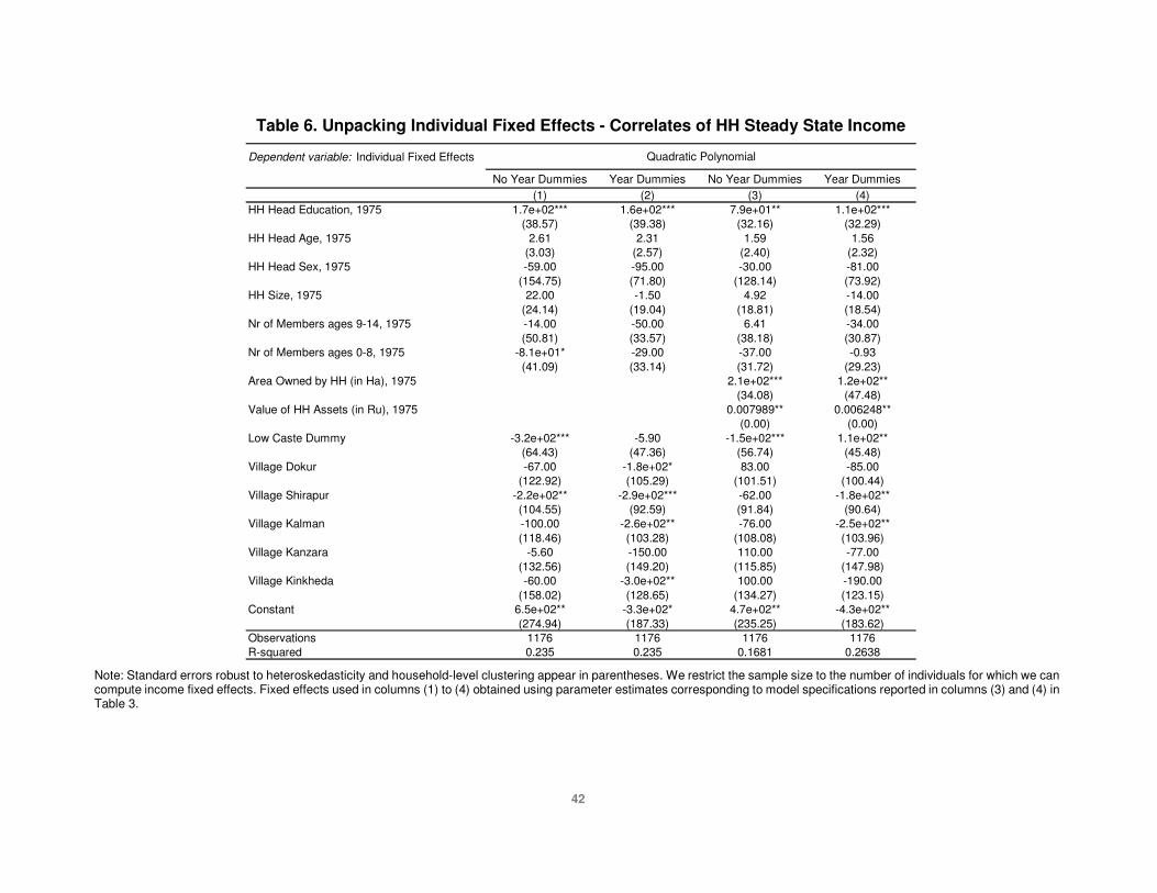
42
Table 6. Unpacking Individual Fixed Effects - Correlates of HH Steady State Income
Dependent variable: Individual Fixed Effects
No Year Dummies Year Dummies No Year Dummies Year Dummies(1) (2) (3) (4)
HH Head Education, 1975 1.7e+02*** 1.6e+02*** 7.9e+01** 1.1e+02***(38.57) (39.38) (32.16) (32.29)
HH Head Age, 1975 2.61 2.31 1.59 1.56(3.03) (2.57) (2.40) (2.32)
HH Head Sex, 1975 -59.00 -95.00 -30.00 -81.00(154.75) (71.80) (128.14) (73.92)
HH Size, 1975 22.00 -1.50 4.92 -14.00(24.14) (19.04) (18.81) (18.54)
Nr of Members ages 9-14, 1975 -14.00 -50.00 6.41 -34.00(50.81) (33.57) (38.18) (30.87)
Nr of Members ages 0-8, 1975 -8.1e+01* -29.00 -37.00 -0.93(41.09) (33.14) (31.72) (29.23)
Area Owned by HH (in Ha), 1975 2.1e+02*** 1.2e+02**(34.08) (47.48)
Value of HH Assets (in Ru), 1975 0.007989** 0.006248**(0.00) (0.00)
Low Caste Dummy -3.2e+02*** -5.90 -1.5e+02*** 1.1e+02**(64.43) (47.36) (56.74) (45.48)
Village Dokur -67.00 -1.8e+02* 83.00 -85.00(122.92) (105.29) (101.51) (100.44)
Village Shirapur -2.2e+02** -2.9e+02*** -62.00 -1.8e+02**(104.55) (92.59) (91.84) (90.64)
Village Kalman -100.00 -2.6e+02** -76.00 -2.5e+02**(118.46) (103.28) (108.08) (103.96)
Village Kanzara -5.60 -150.00 110.00 -77.00(132.56) (149.20) (115.85) (147.98)
Village Kinkheda -60.00 -3.0e+02** 100.00 -190.00(158.02) (128.65) (134.27) (123.15)
Constant 6.5e+02** -3.3e+02* 4.7e+02** -4.3e+02**(274.94) (187.33) (235.25) (183.62)
Observations 1176 1176 1176 1176R-squared 0.235 0.235 0.1681 0.2638
Quadratic Polynomial
Note: Standard errors robust to heteroskedasticity and household-level clustering appear in parentheses. We restrict the sample size to the number of individuals for which we can compute income fixed effects. Fixed effects used in columns (1) to (4) obtained using parameter estimates corresponding to model specifications reported in columns (3) and (4) in Table 3.

43
Graph [A1]: Simulated Income Dynamics for Median, 10th percentile and 90th percentile of fixed effects All Model Specifications: TSLS GMM Estimates - Linear, Quadratic and Cubic
Panel A – No Year Dummies – Linear, Quadratic and Cubic
-100
00
1000
2000
3000
Cur
rent
Inco
me
-500 0 500 1000 1500 2000 2500 3000Lagged Income
Income: 10th percentile Income: medianIncome: 90th percentile 45-degree line
-100
00
1000
2000
3000
Cur
rent
Inco
me
-500 0 500 1000 1500 2000 2500 3000Lagged Income
Income: 10th percentile Income: medianIncome: 90th percentile 45-degree line
-400
0-2
000
020
0040
00C
urre
nt In
com
e
-500 0 500 1000 1500 2000 2500 3000Lagged Income
Income: 10th percentile Income: medianIncome: 90th percentile 45-degree line
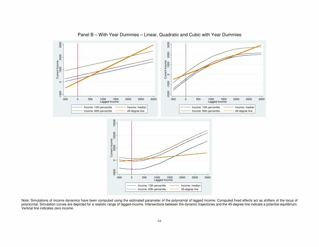
44
Panel B – With Year Dummies – Linear, Quadratic and Cubic with Year Dummies
-100
00
1000
2000
3000
Cur
rent
Inco
me
-500 0 500 1000 1500 2000 2500 3000Lagged Income
Income: 10th percentile Income: medianIncome: 90th percentile 45-degree line
-200
0-1
000
010
0020
0030
00C
urre
nt In
com
e
-500 0 500 1000 1500 2000 2500 3000Lagged Income
Income: 10th percentile Income: medianIncome: 90th percentile 45-degree line
-5
000
050
0010
000
1500
0C
urre
nt In
com
e
-500 0 500 1000 1500 2000 2500 3000Lagged Income
Income: 10th percentile Income: medianIncome: 90th percentile 45-degree line
Note: Simulations of income dynamics have been computed using the estimated parameter of the polynomial of lagged income. Computed fixed effects act as shifters of the locus of polynomial. Simulation curves are depicted for a realistic range of lagged-income. Intersections between the dynamic trajectories and the 45-degree line indicate a potential equilibrium. Vertical line indicates zero income.

45
Graph [A2]: Parsimonious IV Model – Simulated Income Dynamics with Median, 10th percentile and 90th percentile of fixed effects Model Specification: Fuller Estimates with Two Instruments [( Rainfall x Land ) and ( Rainfall x Kids )] – Quadratic Polynomial
Model with Year Dummies
Panel A – Fuller Estimates Panel B – Fuller Estimates with IPW Attrition Correction
-200
0-1
000
010
0020
0030
00C
urre
nt In
com
e
-500 0 500 1000 1500 2000 2500 3000Lagged Income
Income: 10th percentile Income: medianIncome: 90th percentile 45-degree line
-100
00
1000
2000
3000
Cur
rent
Inco
me
-500 0 500 1000 1500 2000 2500 3000Lagged Income
Income: 10th percentile Income: medianIncome: 90th percentile 45-degree line
Note: Panel A reports Fuller estimates for the quadratic polynomial model with year dummies. Panel B reports Fuller estimates with Inverse Probability Weights correction. IPW weights are computed as the inverse of the predicted probability of attrition in a given wave. Individual, household and household head characteristics are used as predictors of wave attrition. Simulations of income dynamics have been computed using the estimated parameter of the polynomial of lagged income. Computed fixed effects act as shifters of the locus of polynomial. Simulation curves are depicted for a realistic range of lagged-income. Intersections between the dynamic trajectories and the 45-degree line indicate a potential equilibrium. Vertical line indicates zero income.

46
Graph [A3]: VLS1 and VLS2 Dynamics – Simulated Income Dynamics with Median, 10th percentile and 90th percentile of fixed effectsModel Specification: Fuller Estimates – Quadratic Polynomial Model with Year Dummies by Panel Period
Panel A – VLS1 (1975-1983) Panel B – VLS2 (2001-2004)
-100
00
1000
2000
3000
Cur
rent
Inco
me
-500 0 500 1000 1500 2000 2500 3000Lagged Income
Income: 10th percentile Income: medianIncome: 90th percentile 45-degree line
-200
00
2000
4000
6000
Cur
rent
Inco
me
-500 0 500 1000 1500 2000 2500 3000Lagged Income
Income: 10th percentile Income: medianIncome: 90th percentile 45-degree line
Note: Simulations of income dynamics have been computed using the estimated parameter of the polynomial of lagged income. Computed fixed effects act as shifters of the locus of polynomial. Simulation curves are depicted for a realistic range of lagged-income. Intersections between the dynamic trajectories and the 45-degree line indicate a potential equilibrium. Vertical line indicates zero income. Estimation methodology drops two years from each panel period, 1975-76 and 2001-2002 in VLS1 and VLS2 respectively.

47
Table A1. Robustness Checks: ‘Weak’ IV Robust Estimators – TSLS LIML and TSLS Fuller
Linear Polynomial
Quadratic Polynomial
Cubic Polynomial
Linear Polynomial
Quadratic Polynomial
Cubic Polynomial
(1) (2) (3) (4) (5) (6)�Y t-1 0.502424* 2.034827** -1.200000 0.477534* 1.867273** 1.886554**
(0.271) (0.954) (23.849) (0.261) (0.839) (0.871)�Y t-1
2 -0.000404* 0.003986 -0.000369* -0.000458(0.000) (0.032) (0.000) (0.000)
�Y t-13 -0.000001 0.000000
(0.000) (0.000)�Year: 1977 60 -21.0000 -360.0000 65.0000 -7.4000 5.0278
(-57.666) (98.245) (2,457.988) (55.944) (90.013) (78.072)�Year: 1978 -93 -1.6e+02** -660.0000 -89.0000 -1.5e+02** -1.4e+02**
(-71.381) (78.186) (3,650.417) (69.865) (72.388) (65.317)�Year: 1979 8.126988 -22.0000 -70.0000 7.9915 -19.0000 -18.0000
(-42.394) (54.435) (375.374) (41.799) (51.933) (48.933)�Year: 1980 -85 -59.0000 80.0000 -84.0000 -61.0000 -65.0000
(-54.861) (63.530) (1,009.924) (54.422) (61.575) (59.156)�Year: 1981 88 120.0000 -14.0000 86.0000 110.0000 110.0000
(-60.889) (88.267) (975.295) (59.837) (83.611) (84.074)�Year: 1982 1.4e+02*** 1.3e+02* 330.0000 1.4e+02*** 1.3e+02* 1.3e+02*
(-43.105) (73.068) (1,471.271) (42.286) (68.516) (69.459)�Year: 1983 -2.2e+02*** -2.3e+02*** -400.0000 -2.2e+02*** -2.3e+02*** -2.2e+02***
(-57.338) (52.672) (1,280.467) (56.269) (50.150) (48.464)�Year: 2003 -8.5e+02*** -8.5e+02*** 1400.0000 -8.4e+02*** -8.4e+02*** -8.8e+02***
(-208.418) (259.896) (17,000.000) (204.824) (245.629) (249.309)�Year: 2004 7.2e+02** 550.0000 -2000.0000 7.0e+02** 5.4e+02* 5.9e+02**
(-303.245) (341.497) (20,000.000) (295.831) (321.720) (286.611)Observations 2260 2260 2260 2260 2260 2260R-squared -0.5354 -1.7527 -159.6338 -0.4945 -1.4715 -1.2559First-Stage DiagnosticsNumber of Instruments 3 3 3 3 3 3Cragg-Donald F-Statistic 15.7872 3.515 0.0028 15.7872 3.515 0.0028F-Statistic - �Yt-1 7.9327 7.9327 7.9327 7.9327 7.9327 7.9327F-Statistic - �Yt-1
2 8.0919 8.0919 8.0919 8.0919F-Statistic - �Yt-1
3 7.0878 7.0878Second-Stage DiagnosticsAnderson-Rubin F stat 5.092 5.092 5.092 5.092 5.092 5.092Prob > F 0.002 0.002 0.002 0.002 0.002 0.002Hansen J Statistic (overidentification) 3.446 0.348 - 3.535 0.379 -Prob > chi-squared 0.179 0.555 - 0.171 0.538 -
IV LIML Estimates IV Fuller EstimatesDependent variable: �Yt
Note: Standard errors robust to heteroskedasticity and ‘original’ household-level clustering appear in parentheses. Income measured in 1975 Rupees per adult equivalent. Anderson Rubin F statistic tests the null hypothesis that the endogenous regressors are jointly insignificant in structural equation. Hansen J Statistic, reported for overidentified models tests null hypothesis that the excluded instruments are uncorrelated with the structural equation error. Cragg-Donald F-Statistics reported includes Kleibergen-Paap rank correction. Cragg-Donald 'Weak IV' statistic tests for the null hypothesis that instruments are strongly correlated with the set of endogenous variables.

48
Table A2. Robustness Checks – Parsimonious IV Set: Interactions ( Rainfall x Land ) and ( Rainfall x Kids )
GMM or LIML Estimators Fuller Estimator GMM or LIML Estimators Fuller Estimator
(1) (2) (3) (4)�Y t-1 2.120567** 1.926574** 2.155082 1.531708*
(0.908) (0.788) (1.748) (0.798)�Y t-1
2 -0.000439** -0.000395** -0.000474 -0.000301(0.000) (0.000) (0.001) (0.000)
�Year: 1977 -19.0000 -4.9000 -14.0000 17.0000(94.943) (86.906) (109.716) (87.593)
�Year: 1978 -1.6e+02** -1.5e+02** -1.5e+02* -1.2e+02*(77.627) (71.703) (77.972) (63.890)
�Year: 1979 -25.0000 -22.0000 -36.0000 -20.0000(54.682) (51.970) (74.304) (50.860)
�Year: 1980 -56.0000 -59.0000 -69.0000 -79.0000(64.502) (62.088) (79.734) (64.260)
�Year: 1981 110.0000 110.0000 190.0000 160.0000(90.439) (85.096) (163.178) (126.450)
�Year: 1982 1.3e+02* 1.3e+02* 71.0000 89.0000(75.813) (70.433) (129.007) (92.980)
�Year: 1983 -2.3e+02*** -2.2e+02*** -2.1e+02*** -2.1e+02***(54.213) (51.392) (77.258) (59.359)
�Year: 2003 -8.3e+02*** -8.2e+02*** -9.4e+02** -9.0e+02***(272.697) (254.679) (446.218) (328.488)
�Year: 2004 500.0000 490.0000 110.0000 320.0000(385.892) (357.504) (999.787) (519.470)
Observations 8279 8279 8279 8279R-squared -1.9732 -1.6124 -3.5570 -1.6163First-Stage DiagnosticsNumber of Instruments 2 2 2 2Cragg-Donald F-Statistic 4.2201 4.2201 0.7536 0.7536F-Statistic - �Yt-1 10.138 10.138 5.6812 5.6812F-Statistic - �Yt-1
2 9.6768 9.6768 4.2166 4.2166Second-Stage DiagnosticsAnderson-Rubin F stat 7.216 7.216 4.784 4.784Prob > F 0.001 0.001 0.009 0.009
With Attrition CorrectionQuadratic Polynomial ModelDependent variable: �Yt
Note: Parsimonious instruments are as follows: (Rainfall x Land Operated (Ha)) and (Rainfall x Nr Kids 0-8). Columns (3) and (4) report estimates with IPW attrition correction. Inverse probability weights are computed as the inverse of the predicted probability of attrition in a given wave. Individual, household and household head characteristics are used as predictors of wave attrition. Standard errors robust to heteroskedasticity and ‘original’ household-level clustering appear in parentheses. Income measured in 1975 Rupees per adult equivalent. Anderson Rubin F statistic tests the null hypothesis that the endogenous regressors are jointly insignificant in structural equation. Hansen J Statistic not defined since both models are only just-identified Cragg-Donald F-Statistics reported includes Kleibergen-Paap rank correction. Cragg-Donald 'Weak IV' statistic tests for the null hypothesis that instruments are strongly correlated with the set of endogenous variables.
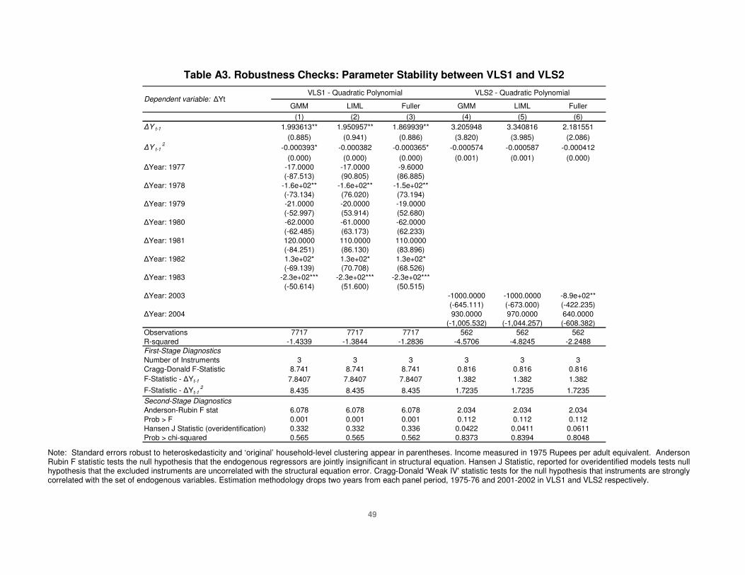
49
Table A3. Robustness Checks: Parameter Stability between VLS1 and VLS2
GMM LIML Fuller GMM LIML Fuller(1) (2) (3) (4) (5) (6)
�Y t-1 1.993613** 1.950957** 1.869939** 3.205948 3.340816 2.181551(0.885) (0.941) (0.886) (3.820) (3.985) (2.086)
�Y t-12 -0.000393* -0.000382 -0.000365* -0.000574 -0.000587 -0.000412
(0.000) (0.000) (0.000) (0.001) (0.001) (0.000)�Year: 1977 -17.0000 -17.0000 -9.6000
(-87.513) (90.805) (86.885)�Year: 1978 -1.6e+02** -1.6e+02** -1.5e+02**
(-73.134) (76.020) (73.194)�Year: 1979 -21.0000 -20.0000 -19.0000
(-52.997) (53.914) (52.680)�Year: 1980 -62.0000 -61.0000 -62.0000
(-62.485) (63.173) (62.233)�Year: 1981 120.0000 110.0000 110.0000
(-84.251) (86.130) (83.896)�Year: 1982 1.3e+02* 1.3e+02* 1.3e+02*
(-69.139) (70.708) (68.526)�Year: 1983 -2.3e+02*** -2.3e+02*** -2.3e+02***
(-50.614) (51.600) (50.515)�Year: 2003 -1000.0000 -1000.0000 -8.9e+02**
(-645.111) (-673.000) (-422.235)�Year: 2004 930.0000 970.0000 640.0000
(-1,005.532) (-1,044.257) (-608.382)Observations 7717 7717 7717 562 562 562R-squared -1.4339 -1.3844 -1.2836 -4.5706 -4.8245 -2.2488First-Stage DiagnosticsNumber of Instruments 3 3 3 3 3 3Cragg-Donald F-Statistic 8.741 8.741 8.741 0.816 0.816 0.816F-Statistic - �Yt-1 7.8407 7.8407 7.8407 1.382 1.382 1.382F-Statistic - �Yt-1
2 8.435 8.435 8.435 1.7235 1.7235 1.7235Second-Stage DiagnosticsAnderson-Rubin F stat 6.078 6.078 6.078 2.034 2.034 2.034Prob > F 0.001 0.001 0.001 0.112 0.112 0.112Hansen J Statistic (overidentification) 0.332 0.332 0.336 0.0422 0.0411 0.0611Prob > chi-squared 0.565 0.565 0.562 0.8373 0.8394 0.8048
Dependent variable: �YtVLS1 - Quadratic Polynomial VLS2 - Quadratic Polynomial
Note: Standard errors robust to heteroskedasticity and ‘original’ household-level clustering appear in parentheses. Income measured in 1975 Rupees per adult equivalent. Anderson Rubin F statistic tests the null hypothesis that the endogenous regressors are jointly insignificant in structural equation. Hansen J Statistic, reported for overidentified models tests null hypothesis that the excluded instruments are uncorrelated with the structural equation error. Cragg-Donald 'Weak IV' statistic tests for the null hypothesis that instruments are strongly correlated with the set of endogenous variables. Estimation methodology drops two years from each panel period, 1975-76 and 2001-2002 in VLS1 and VLS2 respectively.