the richer representation the better registration

5036 IEEE TRANSACTIONS ON IMAGE PROCESSING, VOL. 22, NO. 12, DECEMBER 2013

The Richer Representation the Better RegistrationMohammad Rouhani, Student Member, IEEE, and Angel Domingo Sappa, Senior Member, IEEE

Abstract— In this paper, the registration problem is formulatedas a point to model distance minimization. Unlike most of theexisting works, which are based on minimizing a point-wisecorrespondence term, this formulation avoids the correspondencesearch that is time-consuming. In the first stage, the targetset is described through an implicit function by employinga linear least squares fitting. This function can be either animplicit polynomial or an implicit B-spline from a coarse to finerepresentation. In the second stage, we show how the obtainedimplicit representation is used as an interface to convert point-to-point registration into point-to-implicit problem. Furthermore,we show that this registration distance is smooth and can beminimized through the Levengberg–Marquardt algorithm. Allthe formulations presented for both stages are compact and easyto implement. In addition, we show that our registration methodcan be handled using any implicit representation though some arecoarse and others provide finer representations; hence, a tradeoffbetween speed and accuracy can be set by employing the rightimplicit function. Experimental results and comparisons in 2Dand 3D show the robustness and the speed of convergence of theproposed approach.

Index Terms— Rigid registration, surface fitting, implicitpolynomials, implicit B-splines, registration error estimation,residual error minimization, Levenberg-Marquadt algorithm.

I. INTRODUCTION

OBJECT representation and point set registration both arecommon problems in computer vision. In general, they

are tackled as standalone problems and studied separately. Thecurrent work places a bridge that connects both problems look-ing for an efficient solution. Being inspired by the ComputerGraphics (CG) and Computer Aided Design (CAD) communi-ties a compact object representation is adopted to reformulatethe registration problem in a unified representation-registrationframework.

The object representation field focuses on developing com-pact models that allow to deal with large amount of data.Nowadays, due to the improvement in 3D scanners, we aresurrounded by a high amount of raw data as 2D or 3D cloudof points, and having a smooth and compact representation isone of the important objectives that benefit computer visionapplications. In the current work we exploit implicit repre-sentations, including Implicit Polynomial (IP) and Implicit

Manuscript received January 2, 2013; revised June 3, 2013 and July 31,2013; accepted August 24, 2013. Date of publication September 11, 2013;date of current version October 2, 2013. This work was supported by theGovernment of Spain under Projects TIN2011-25606 and TIN2011-29494-C03-02. The associate editor coordinating the review of this manuscript andapproving it for publication was Prof. Gang Hua.

M. Rouhani is with Morpheo, INRIA Rhône-Alpes, Grenoble 38000, France(e-mail: [email protected]).

A. D. Sappa is with the Computer Vision Center, Bellaterra 08193, Spain(e-mail: [email protected]).

Color versions of one or more of the figures in this paper are availableonline at http://ieeexplore.ieee.org.

Digital Object Identifier 10.1109/TIP.2013.2281427

B-Spline (IBS), to tackle the registration of two clouds ofpoints.

The registration problem, on the other hand, aims at findingthe best transformation that places both the given source setand its corresponding target set into the same reference systemin order to minimize their distance. This transformation,depending on the application, could be either rigid or non-rigid. The rigid transformation only considers rotation andtranslation parameters to move the source set [1]. The non-rigid transformation, on the contrary, allows more degrees offreedom for deforming the source set in order to minimizethe distance between the two sets [2], [3]. The current workpresents a novel rigid registration distance approximation thatcan benefit both rigid and non-rigid registration. It is anextension of a preliminary version [4] where only IPs areused to describe the target set. In this work we show thatthe proposed point to model distance minimization can bealso used with a more flexible implicit representation, ImplicitB-Spline (IBS) [5]. This flexible representation (IBS) can beused to induce a fast and robust registration error.

The best rotation and translation could be roughly approx-imated by the Principle Component Analysis (PCA). Indeed,PCA just finds the major axes of each cloud of points andthen aligns these axes by translating the origin followed bya rotation; hence, it just provides a coarse registration. Theregistration methods, in general, can be divided into two maincategories, namely coarse and fine registration, where the latterprovides a more precise alignment. The coarse registration isnot very precise but it can be used as initialization for a fineregistration method. Gelfand et. al. in [6], for instance, presenta coarse registration using a branch-and-bound algorithm toinitialize a fine registration algorithm.

In general, fine registration approaches find the best rigidtransformation by iterating two steps. In the first step thecorrespondences between the given source points and thetarget points are sought in order to compute the registrationresidual error. Then, in the second step, the best set ofparameters are found by minimizing this residual error. Thesetwo steps are repeated until some convergence criteria isreached. The Iterative Closest Point (ICP) algorithm is oneof the classical registration approaches following this two-step scheme. It has been originally presented in [7] and [11]and several improvements have been proposed in the literaturelooking for more efficient and robust solutions (e.g., [8]–[10]).Note that in most of these approaches the correspondencesearch is performed at the point level and it makes the wholeprocess computationally expensive.

Some effort to link the registration with the representationproblem has been made by using high level representations inorder to avoid the correspondence search. Implicit polynomialshave been exploited in [11] to represent both the source set and

1057-7149 © 2013 IEEE

ROUHANI AND SAPPA: RICHER REPRESENTATION THE BETTER REGISTRATION 5037

Fig. 1. Using an interface for point sets registration: (a) Initial position of source (+) and target (o) sets; (b) Source set (+) and target set represented byan IBS; (c) Registration result of source set (+) and the IBS; (d) The same result but represented by using the target set (o) and transformed source set (+).

target set. Probabilistic representations, like GMM, have beenused to describe both source set and target set (e.g. [12]– [14]).In [15]– [17] the point-wise problem is avoided by using eitherthe distance field of the target set or the distance fields of bothtarget and source sets. More details about all these approachesare given in the next section.

The current work proposes a novel and fast registrationapproach that exploits a compact and smooth representationas an interface to avoid the point-to-point correspondencesearch. It consists of two main stages: in the first stage, animplicit representation is provided to describe the target set.An optimal implicit function is fitted using the least squaresform, hence it is quite fast. Although any implicit functioncan be used in the current work we just show the usage ofimplicit polynomials and implicit B-splines, which can beindistinctly adopted in the proposed registration framework.In the second stage, we use a fast distance estimation todefine the residual errors. This distance is induced by thefitted implicit function from the first stage. The final registra-tion distance is differentiable with respect to the registrationparameters and allows solving the problem through a gradientbased optimization algorithm. Due to the compactness of theimplicit representation the whole scheme can be used in acoarse-to-fine framework. The rest of this paper is organizedas follows: Section II details related work. Section III presentsboth the proposed representation and registration approaches.Experimental results and comparisons with state of the artare presented in Section IV. Finally, conclusions are given inSection V.

II. MOTIVATION AND RELATED WORK

Let us consider two sets of points, referred to as source set(data) S = {si }Ns

1 , and target set (model) T = {ti }Nt1 (see

Fig. 1(a)). In the rigid case, the registration problem aims atfinding the best rotation and translation in order to take thesource set as close as possible to the target set. For this purposemany point-to-point comparisons must be executed in orderto measure the closeness. For the non-structured case it willtake O(Ns Nt ) just for obtaining the distance measurement.Although more elaborated solutions using data structure havebeen introduced, our proposal is to replace the target set witha proper interface that accelerates the distance measurement(Fig. 1). Then the optimal configuration can be found throughmeasuring the point distances from this interface.

In order to work with an interface, instead of a point cloud,a proper geometric model should be used. Triangle meshesand parametric NURBS are among the common tools in thesedomains, but they suffer from either the geometry limitationor the parametrization problem. Implicit functions, on the con-trary, provide a flexible representation without requiring anyparametrization over the point cloud. They describe objectsin 2D/3D through the level set where the function reacheszero. Implicit Polynomial (IP) [18] is one of the simplestchoices for the function space F , since it is made out ofsimple monomials. IPs can easily describe a given objectthrough a set of coefficients, but they are not flexible enough.In other words, IPs suffer from the outliers created around thepoint set, which are due to their non-compact supports. RadialBasis Functions (RBFs) [19] provide another solution spacefor implicit representations. They are smooth and flexible, butsmall changes in the coefficient vector can lead to a globalchange in the whole object.

In this work Implicit B-Splines (IBSs) beside implicitpolynomials are employed to represent the target set. IBSproposes a smooth and flexible representation without anyneed of parametrization [20]. Moreover, it is constructed outof B-spline basis functions, which have compact supports.Hence they have local control (i.e, changes in one coefficientchanges the local behavior of the object). Fig. 1(b) illustratesthe flexibility of IBSs to describe a complex 3D shape. In thecurrent work the optimal IBS/IP is easily obtained by means ofan extension of the 3L algorithm [18], which is a fast algebraicfitting method formulated as linear least squares.

IP and IBS both provide an overall representation for thetarget points. Since both are in a linear implicit form, they canbe easily computed. IP provides a fast and simple represen-tation while IBS results in a more accurate description. Oncethe target set has been described by a proper implicit functionthe registration problem can be tackled in a point-to-modelscheme, which leads to a correspondence free registrationmethod. Moreover, a tradeoff between the speed and accuracycan be met by employing a coarse or fine implicit represen-tation. Point-to-model schemes have been already studied inthe literature by considering different representations for targetand source sets. These methods can be broadly classified asprobabilistic-based and distance-field-based approaches.

Probabilistic approaches represent each given set by aprobabilistic model like multivariate t-distributions [12] orGaussian Mixture Model (GMM) [13], [21]; hence, the


registration problem becomes a problem of aligning two mix-tures, which can be solved in the quasi-Newton optimizationframework. These approaches are highly dependent on thenumber of mixtures used for modeling the point sets. Hence, auser defined number of mixtures, or as many as the number ofpoints, is required. Moreover, although these methods do notrequire any correspondence search, all points in the model areimplicitly considered as a potential correspondence (almost allthe points contribute to the GMM construction).

On the contrary to the previous approaches, distance fieldhas been used as an implicit representation, which providesinformation over the whole domain. The method presentedin [15] overcomes the non-differentiable nature of ICP byusing a differentiable distance transform—Chamfer distance.The error function derived from that distance field is a smoothfunction, and its derivatives can be analytically computed;hence it can be minimized through the Levenberg-Marquardtalgorithm (LMA) to find the optimal registration parameters.The distance field used in [15] is a discrete field and itsderivatives used in LMA are not precise enough. In [16] alocal quadratic approximation of the distance function, basedon the curvature information, is presented. Unfortunately,computing the principal curvatures over the point cloud iscomputationally expensive and sensitive to noise. Finally, [17]proposes a distance field approximation by using an implicitpolynomial [22]. This IP is considered to define a gradient flowthat drives the source towards the target without using point-wise correspondences. Although fast, the proposed gradientflow is not precise, especially close to the boundaries.

In the current work a novel approach is presented toreformulate the point-to-point registration as a point-to-modelproblem. In the first stage, an implicit function is constructedto represent the target points. This representation is either animplicit polynomial or implicit B-spline that can be rapidlyconstructed. As a contribution a linear least squares fittingalgorithm is adopted to find the optimal IBS that describesthe target set more accurate than IP. Fig. 1(a) illustrates theinitial position of the source and target sets. The IBS zero setrepresenting the given target set is depicted in Fig. 1(b). Inthe second stage this implicit function (either IP or IBS) isused as an interface during the registration process. Fig. 1(c)presents the registration results from the source set and theIBS. Note that the optimal registration result is obtained asshown in Fig. 1(d). In this figure source set and target set aredepicted again as point clouds.

III. PROPOSED METHOD

This section presents the main contributions of the currentwork. First, the target set is described through an implicitfunction like implicit polynomial (IP) or implicit B-spline(IBS). We employ the 3L algorithm to find the optimal IPand adapt it to find the optimal IBS. IP and IBS are bothin implicit forms so the target points are not required to beparametrized. Moreover, both classes are linear with respectto their coefficient vectors; so, we employ the same techniqueto find an optimal IP or IBS. In the second part, the obtainedimplicit representation is used for aligning two sets of points.

The distance used to measure the alignment error is a fastdistance estimation induced by the fitted implicit function.The accumulated error is in the non-linear least squaresform, and hence can be optimized by the Levenberg-MarquadtAlgorithm. This minimization stage is iterated until conver-gence is reached. It should be highlighted that the formulationspresented in the second stage are completely independent ofthe choice for the representation in the first stage. So, it is upto the user to chose either a simple and fast representation likeIP or a more flexible and precise one like IBS.

A. Object Representation

An object in 2D/3D can be easily described by a cloud ofpoints sampled from the object surface. This point cloud canbe enriched by knowing the point connections, for instancethrough the corresponding triangle mesh. Unfortunately, thisrepresentation has a geometry limitation and requires lots ofmemory to deliver a fine enough representation. Moreover,point level representation induces expensive point-wise com-putations for our registration problem. In order to cope withthese limitations, the target point cloud is described through animplicit function. An implicit function f describes the objectof interest implicitly through its zero set including those pointswhere f obtains zero; i.e., Z f = {x ∈ R

k : f (x) = 0}. Giventhe target points T = {ti }Nt

1 an optimal implicit function canbe sought by minimizing the distance between the target pointsand the zero set of this function. This implicit function f canbe easily chosen as an implicit polynomial defined as:

f (x) = f (x, y) =∑

(i+ j )�d{i, j }�0

ci, j x i y j = 0, (1)

where d is the polynomial degree. An IP is a simple descrip-tion of the point set through a set of monomials and coeffi-cients. The higher the IP degree is the more degree of freedomare captured by the IP; but then, the outliers created by theIP zero set cannot be easily avoided. In our experiments weuse an IP up to 7th degree that can roughly describe the pointcloud. In order to have a finer and precise representation, animplicit B-Spline can be alternatively used, which is definedas a combination of the tensor products of 1D basis functions:

f (x) = f (x, y) =M∑

i=1

N∑

j=1

ci, j Bi(x)B j (y), (2)

where Bi (x) B j (y) are the spline basis functions, and thematrix [ci, j ]M×N is the control lattice (coefficients) controllingthe shape of the IBS [5]. For the sake of simplicity we considerM = N , then the basis functions Bi (x) and B j (y) have thesame behavior, though defined in different domains. Similarly,the basis functions in 3D are tensor products of three 1Dbasis functions. In general, IBSs provide smooth and flexiblerepresentations in an implicit form. Constructed through a setof basis functions with compact supports, IBS can be locallycontrolled in contrast to implicit polynomials and radial basisfunctions.

We exploit the simplicities and flexibilities of IPs and IBSsto reformulate the registration problem. In the first stage of our


registration method the target set is replaced by an IP or IBSby employing the same fitting algorithm. It should be noticedthat IP and IBS, despite their different formulations, have asimilar form and both of them can be linearly described basedon the their coefficients:

f (x) = cT m(x) = m(x)T c, (3)

where c is the coefficient vector containing the IP or IBScoefficients and m(x) is the basis vector containing the IPor IBS basis functions. The basis vector for IP comprises themonomials in the form of xi y j :

m(x) = [1, x, y, x2, xy, y2, x3, x2 y, ..., yd]T . (4)

For the case of implicit B-Spline the basis vector contains thebasis functions in the term of tensor products Bi (x)B j (y):

m(x) = [B1(x)B1(y), ..., B1(x)BN (y), ..., BN (x)BN (y)]T .(5)

Note that the coefficient vector must respect the same orderas the basis vector. Then, the inner product of the coefficientvector and the basis vector (either IP or IBS) defines theimplicit function (IP/IBS) as already defined in (1) and (2).

Surface reconstruction techniques concern finding the opti-mal coefficient vectors to describe the given point cloud. Inthe current work, we employ the 3L algorithm [18] to findthe optimal coefficients in order to describe the target pointcloud T = {ti }Nt

1 . Moreover, we adapt the original algorithmto find the optimal IBS coefficients still in a linear leastsquares framework. The decision whether to use IP or IBSto represent the given target set depends on its geometricalcomplexity. In other words, the user should select which oneis the best option for the given target set: if a simple overalldescription is enough, then IP can be used; otherwise, IBS ispreferred in order to capture more details of target point cloud.In this section we show that a common fitting frameworkand formulation can be used to find the optimal IP or IBSdescription and this is why we present both formulations at thesame time. Later in section III-B we show that our proposedformulation for point to model registration is independent ofthe implicit representation of the target points, so both IP andIBS can be used. Of course employing a low resolution IPduring the registration leads us to a coarse solution, while ahigh resolution IBS (afterwards) can deliver a better estimationof the registration parameters.

The 3L algorithm considers the given target points T0 = Tas well as its inner and outer offsets {T+δ,T−δ}. The optimalfunction f (either IP or IBS) is found such that it obtains zeroin the original set as well as ±ε in the additional offsets. Then,the objective function F(c) = ‖M3Lc − b‖2 is considered tobe minimized, where:

M3L =⎡

⎣MT−δMT0

MT+δ

⎤

⎦ , b =⎡

⎣−ε0

+ε

⎤

⎦ . (6)

The monomial matrices MT0 and MT±δ are constructed fromthe basis vectors computed in the original set T0 and its offsetsT±δ respectively. In fact each row in these matrices is madeout of the basis functions presented in (4) or (5) dependingon whether IP or IBS is selected for the description.

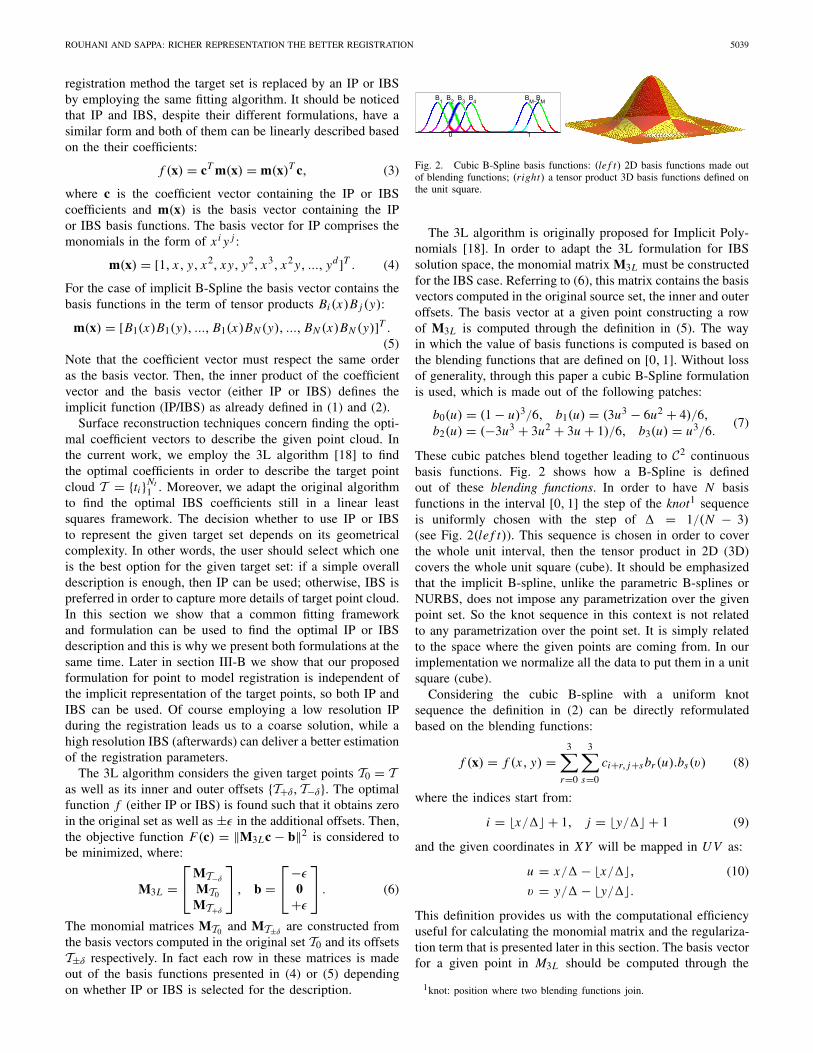
Fig. 2. Cubic B-Spline basis functions: (le f t) 2D basis functions made outof blending functions; (right) a tensor product 3D basis functions defined onthe unit square.

The 3L algorithm is originally proposed for Implicit Poly-nomials [18]. In order to adapt the 3L formulation for IBSsolution space, the monomial matrix M3L must be constructedfor the IBS case. Referring to (6), this matrix contains the basisvectors computed in the original source set, the inner and outeroffsets. The basis vector at a given point constructing a rowof M3L is computed through the definition in (5). The wayin which the value of basis functions is computed is based onthe blending functions that are defined on [0, 1]. Without lossof generality, through this paper a cubic B-Spline formulationis used, which is made out of the following patches:

b0(u) = (1 − u)3/6, b1(u) = (3u3 − 6u2 + 4)/6,b2(u) = (−3u3 + 3u2 + 3u + 1)/6, b3(u) = u3/6.

(7)

These cubic patches blend together leading to C2 continuousbasis functions. Fig. 2 shows how a B-Spline is definedout of these blending functions. In order to have N basisfunctions in the interval [0, 1] the step of the knot1 sequenceis uniformly chosen with the step of � = 1/(N − 3)(see Fig. 2(le f t)). This sequence is chosen in order to coverthe whole unit interval, then the tensor product in 2D (3D)covers the whole unit square (cube). It should be emphasizedthat the implicit B-spline, unlike the parametric B-splines orNURBS, does not impose any parametrization over the givenpoint set. So the knot sequence in this context is not relatedto any parametrization over the point set. It is simply relatedto the space where the given points are coming from. In ourimplementation we normalize all the data to put them in a unitsquare (cube).

Considering the cubic B-spline with a uniform knotsequence the definition in (2) can be directly reformulatedbased on the blending functions:

f (x) = f (x, y) =3∑

r=0

3∑

s=0

ci+r, j+s br (u).bs(v) (8)

where the indices start from:

i = �x/�� + 1, j = �y/�� + 1 (9)

and the given coordinates in XY will be mapped in U V as:

u = x/�− �x/��, (10)

v = y/�− �y/��.This definition provides us with the computational efficiencyuseful for calculating the monomial matrix and the regulariza-tion term that is presented later in this section. The basis vectorfor a given point in M3L should be computed through the

1knot: position where two blending functions join.


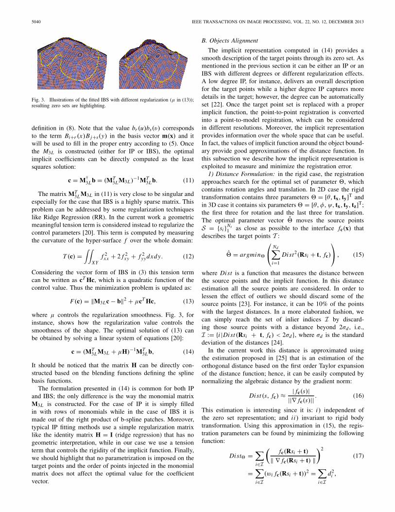
Fig. 3. Illustrations of the fitted IBS with different regularization (μ in (13));resulting zero sets are highlighting.

definition in (8). Note that the value br (u)bs(v) correspondsto the term Bi+r (x)B j+s(y) in the basis vector m(x) and itwill be used to fill in the proper entry according to (5). Oncethe M3L is constructed (either for IP or IBS), the optimalimplicit coefficients can be directly computed as the leastsquares solution:

c = M†3Lb = (MT

3LM3L)−1MT

3Lb. (11)

The matrix MT3LM3L in (11) is very close to be singular and

especially for the case that IBS is a highly sparse matrix. Thisproblem can be addressed by some regularization techniqueslike Ridge Regression (RR). In the current work a geometricmeaningful tension term is considered instead to regularize thecontrol parameters [20]. This term is computed by measuringthe curvature of the hyper-surface f over the whole domain:

T (c) =∫∫

XYf 2x x + 2 f 2

xy + f 2yydxdy. (12)

Considering the vector form of IBS in (3) this tension termcan be written as cT Hc, which is a quadratic function of thecontrol value. Thus the minimization problem is updated as:

F(c) = ‖M3Lc − b‖2 + μcT Hc, (13)

where μ controls the regularization smoothness. Fig. 3, forinstance, shows how the regularization value controls thesmoothness of the shape. The optimal solution of (13) canbe obtained by solving a linear system of equations [20]:

c = (MT3LM3L + μH)−1MT

3Lb, (14)

It should be noticed that the matrix H can be directly con-structed based on the blending functions defining the splinebasis functions.

The formulation presented in (14) is common for both IPand IBS; the only difference is the way the monomial matrixM3L is constructed. For the case of IP it is simply filledin with rows of monomials while in the case of IBS it ismade out of the right product of b-spline patches. Moreover,typical IP fitting methods use a simple regularization matrixlike the identity matrix H = I (ridge regression) that has nogeometric interpretation, while in our case we use a tensionterm that controls the rigidity of the implicit function. Finally,we should highlight that no parametrization is imposed on thetarget points and the order of points injected in the monomialmatrix does not affect the optimal value for the coefficientvector.

B. Objects Alignment

The implicit representation computed in (14) provides asmooth description of the target points through its zero set. Asmentioned in the previous section it can be either an IP or anIBS with different degrees or different regularization effects.A low degree IP, for instance, delivers an overall descriptionfor the target points while a higher degree IP captures moredetails in the target; however, the degree can be automaticallyset [22]. Once the target point set is replaced with a properimplicit function, the point-to-point registration is convertedinto a point-to-model registration, which can be consideredin different resolutions. Moreover, the implicit representationprovides information over the whole space that can be useful.In fact, the values of implicit function around the object bound-ary provide good approximations of the distance function. Inthis subsection we describe how the implicit representation isexploited to measure and minimize the registration error.

1) Distance Formulation: in the rigid case, the registrationapproaches search for the optimal set of parameter �, whichcontains rotation angles and translation. In 2D case the rigidtransformation contains three parameters � = [θ, tx, ty]T andin 3D case it contains six parameters� = [θ, φ,ψ, tx, ty, tz]T;the first three for rotation and the last three for translation.The optimal parameter vector �̂ moves the source pointsS = {si }Ns

1 as close as possible to the interface fc(x) thatdescribes the target points T :

�̂ = argmin�

⎛

⎝Nd∑

i=1

Dist2(Rsi + t, fc)

⎞

⎠ , (15)

where Dist is a function that measures the distance betweenthe source points and the implicit function. In this distanceestimation all the source points are considered. In order tolessen the effect of outliers we should discard some of thesource points [23]. For instance, it can be 10% of the pointswith the largest distances. In a more elaborated fashion, wecan simply reach the set of inlier indices I by discard-ing those source points with a distance beyond 2σd , i.e.,I := {i |Dist (Rsi + t, fc) < 2σd }, where σd is the standarddeviation of the distances [24].

In the current work this distance is approximated usingthe estimation proposed in [25] that is an estimation of theorthogonal distance based on the first order Taylor expansionof the distance function; hence, it can be easily computed bynormalizing the algebraic distance by the gradient norm:

Dist (s, fc) ≈ | fc(s)|||∇ fc(s)|| . (16)

This estimation is interesting since it is: i) independent ofthe zero set representation; and i i) invariant to rigid bodytransformation. Using this approximation in (15), the regis-tration parameters can be found by minimizing the followingfunction:

Dist� =∑

i∈I

(fc(Rsi + t)

‖ ∇ fc(Rsi + t) ‖)2

(17)

=∑

i∈I(wi fc(Rsi + t))2 =

∑

i∈Id2

i ,


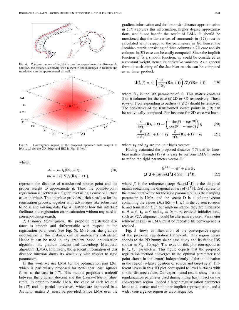
Fig. 4. The level curves of the IBS is used to approximate the distance. Inaddition, the distance sensitivity with respect to small changes in rotation andtranslation can be approximated as well.

Fig. 5. Convergence region of the proposed approach with respect to[θ, tx, ty] for the 2D object and IBS in Fig. 11(top).

where:

di = wi fc(Rsi + t), (18)

wi = 1/‖ ∇ fc(Rsi + t) ‖,represent the distance of transformed source point and theproper weight to approximate it. Thus, the point-to-pointregistration is tackled in a higher level using a curve or surfaceas an interface. This interface provides a rich structure for theregistration process, together with advantages like robustnessto noise and missing data. Fig. 4 illustrates how this interfacefacilitates the registration error estimation without any need tocorrespondence search.

2) Distance Optimization: the proposed registration dis-tance is smooth and differentiable with respect to theregistration parameters (see Fig. 5). Moreover, the gradientinformation of this distance can be analytically calculated.Hence it can be used in any gradient based optimizationalgorithm like gradient descent and Levenberg−Marquardtalgorithm (LMA). Intuitively, the gradient information of thisdistance function shows its sensitivity with respect to rigidparameters.

In this work we use LMA for the optimization part [26],which is particularly proposed for non-linear least squaresforms as the case in (17). This method proposes a tradeoffbetween the gradient descent and the Gauss−Newton algo-rithm. In order to handle LMA, the value of each residualin (17) and its partial derivatives, which are expressed in aJacobian matrix J , must be provided. Since LMA uses the

gradient information and the first order distance approximationin (17) captures this information, higher degree approxima-tions would not benefit the result of LMA. It should bementioned that the derivatives of summands in (17) must becalculated with respect to the parameters in �. Hence, theJacobian matrix consisting of three columns in 2D case and sixcolumns in 3D case can be easily computed. Since the implicitfunction fc is a smooth function, wi could be considered asa constant weight, hence its derivative vanishes. As a generalformula each entry of the Jacobian matrix can be computedas an inner product:

J(i, j) = wi

(∂

∂� j(Rsi + t)

).∇ f (Rsi + t), (19)

where � j is the j th parameter of �. This matrix contains3 or 6 columns for the case of 2D or 3D respectively. Thoserows of J corresponding to outliers (i �∈ I) should be removed.The derivatives of the transformed source points in (19) canbe analytically computed. For instance for 2D case we have:

∂

∂�1(Rsi + t) =

(− sin(θ) − cos(θ)cos(θ) − sin(θ)

)si (20)

∂

∂�2(Rsi + t) = e1

∂

∂�3(Rsi + t) = e2 (21)

where e1 and e2 are the unit basis vectors.Having estimated the proposed distance (17) and its Jaco-

bian matrix through (19) it is easy to perform LMA in orderto refine the rigid parameter vector �:

�k+1 = �k + β�,(JTJ + λdiag(JTJ))� = JTD, (22)

where β is the refinement step; diag(JTJ) is the diagonalmatrix containing the diagonal entries of (JTJ); � representsthe refinement vector for the rigid parameters; λ is the dampingparameter in LMA; and the vector D is a column vectorcontaining the values Dist (Rsi + t, fc) in the current rotationR and translation t. In our implementation they are initializedas θ = 0, tx = 0 and ty = 0; more evolved initializations,such as PCA alignment, could be alternatively used. Parameterrefinement (22) in LMA must be repeated till convergence isreached.

Fig. 5 shows an illustration of the convergence regionof the proposed registration framework. This region corre-sponds to the 2D bunny shape case study and its fitting IBSshown in Fig. 11(top). The axes on this plot correspond to[θ, tx, ty] parameters. This figure depicts that the proposedregistration method converges to the optimal parameter (thepoint shown in the center) independently of the initializationin the region (relative position of source and target sets). Dif-ferent layers in this 3D plot correspond to level surfaces withsimilar distance values. Our experimental results show that theregularization parameter used during fitting has impact on theconvergence region. Indeed a larger regularization parameterleads to a coarser and smoother implicit representation, and awider convergence region as a consequence.


IV. EXPERIMENTAL RESULTS AND COMPARISONS

The experimental results are presented for the proposedregistration scheme using different implicit representations.In the first section, simple IPs are considered to representthe target sets. Despite the simplicity of the representationthe obtained registration results are quite promising. In thefollowing section this representation is promoted to IBSs thatprovide more flexible representations to tackle the registrationof objects with intricate and challenging geometries like theones presented in Fig. 1 and Fig. 12. Note that a singleIP, independently of its degree, cannot properly capture thegeometry of a complex object, such as the one presented inFig. 1, which as a consequence will affect the registrationresult.

The proposed approach has been evaluated using different2D and 3D source sets and target sets from public repositories[27] and [28]. In all the examples, just to visually appreciatethe result, the same set of points is used as source and targetsets. Notice that the proposed approach does not consider thepoints in the target set during the registration, despite thatafter the registration the source points appear on the targetpoints.

In addition to the qualitative evaluation presented with2D contours 3D real objects have been registered with theproposed approach and compared with four techniques (i.e.,[13], [15]– [17]) from the state of the art, together with theclassical ICP [7]. Each technique iterates until one of thesestopping criteria is reaches: if the number of iterations exceedsa maximum bound (#Iter = 40) or the relative registrationerror is smaller than the given threshold (ε < 0.005); relativeregistration error is defined as: ε = |Et − Et−1|/Et , where Et

refers to the registration error between the target and sourceset at iteration t .

On the contrary to the relative registration error, which isan internal measure, an Accumulated Residual Error (ARE) isused during the comparisons. It is computed by measuringthe accumulated error, in a point-wise manner, from thetransformed source set to a reference set. This reference setcorresponds to a highly detailed description of the targetset. It contains the target set and on average is defined by aset of points ten times larger than the target set. Each residualerror is computed by finding the nearest point in between theregistered source set and the reference set.

A. Registration Using IPs

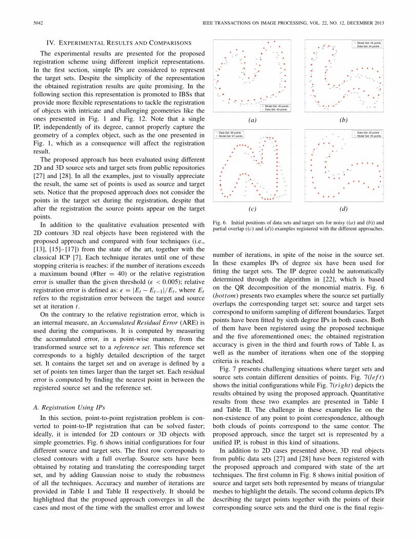
In this section, point-to-point registration problem is con-verted to point-to-IP registration that can be solved faster;ideally, it is intended for 2D contours or 3D objects withsimple geometries. Fig. 6 shows initial configurations for fourdifferent source and target sets. The first row corresponds toclosed contours with a full overlap. Source sets have beenobtained by rotating and translating the corresponding targetset, and by adding Gaussian noise to study the robustnessof all the techniques. Accuracy and number of iterations areprovided in Table I and Table II respectively. It should behighlighted that the proposed approach converges in all thecases and most of the time with the smallest error and lowest

Fig. 6. Initial positions of data sets and target sets for noisy ((a) and (b)) andpartial overlap ((c) and (d)) examples registered with the different approaches.

number of iterations, in spite of the noise in the source set.In these examples IPs of degree six have been used forfitting the target sets. The IP degree could be automaticallydetermined through the algorithm in [22], which is basedon the QR decomposition of the monomial matrix. Fig. 6(bottom) presents two examples where the source set partiallyoverlaps the corresponding target set; source and target setscorrespond to uniform sampling of different boundaries. Targetpoints have been fitted by sixth degree IPs in both cases. Bothof them have been registered using the proposed techniqueand the five aforementioned ones; the obtained registrationaccuracy is given in the third and fourth rows of Table I, aswell as the number of iterations when one of the stoppingcriteria is reached.

Fig. 7 presents challenging situations where target sets andsource sets contain different densities of points. Fig. 7(le f t)shows the initial configurations while Fig. 7(right) depicts theresults obtained by using the proposed approach. Quantitativeresults from these two examples are presented in Table Iand Table II. The challenge in these examples lie on thenon-existence of any point to point correspondence, althoughboth clouds of points correspond to the same contor. Theproposed approach, since the target set is represented by aunified IP, is robust in this kind of situations.

In addition to 2D cases presented above, 3D real objectsfrom public data sets [27] and [28] have been registered withthe proposed approach and compared with state of the arttechniques. The first column in Fig. 8 shows initial position ofsource and target sets both represented by means of triangularmeshes to highlight the details. The second column depicts IPsdescribing the target points together with the points of theircorresponding source sets and the third one is the final regis-


TABLE I

COMPARISONS OF REGISTRATION ERROR (ARE) RESULTS FOR 2D CASES (ICP: ITERATIVE CLOSEST POINT [7];

GMM: GAUSSIAN MIXTURE MODELS [13]; DT: DISTANCE TRANSFORM [15]; GF: GRADIENT FLOW [17];

DA: DISTANCE APPROXIMATION [16]; PA: PROPOSED APPROACH)

TABLE II

NUMBER OF ITERATIONS OF DIFFERENT REGISTRATION

METHODS FOR 2D CASES

Fig. 7. Source and target sets containing different density of points.((a) and (b)) Initial configurations. ((c) and (d)) Final results from theproposed approach.

tration result. The illustration presented in Fig. 8(a)(1strow)corresponds to a source set defined by 811 points. The targetcontains 926 points and is represented by means of a seventhdegree IP. The result obtained with the proposed approach isshown in Fig. 8(c)(1strow). Quantitative information aboutthe data sets, as well as comparisons with other approachesare provided in Table III; the stopping criteria considered inTable I are also used here. A seventh degree IP is used in thesecond row to represent the 745 points of the target set, while

Fig. 8. Public data sets (from [27] and [28]) registered with the proposedapproach and state of the art techniques. (a) Initial set up of the given sourceand target sets represented by means of triangular meshes to highlight details.(b) IPs representing target sets and source points. (c) Results of the proposedregistration approach represented through triangular meshes to make visualevaluation easier.

the source set contains 609 points. Note that after describingthe target set with its fitting IP the target points are no longerconsidered. A fifth degree and a sixth degree IPs are usedin the third and fourth rows, respectively. Fig. 8(c) presentsthe registration obtained with the proposed approach. Statisticsabout their registration process and comparisons with state ofthe art techniques are presented in Table III and Table IV.

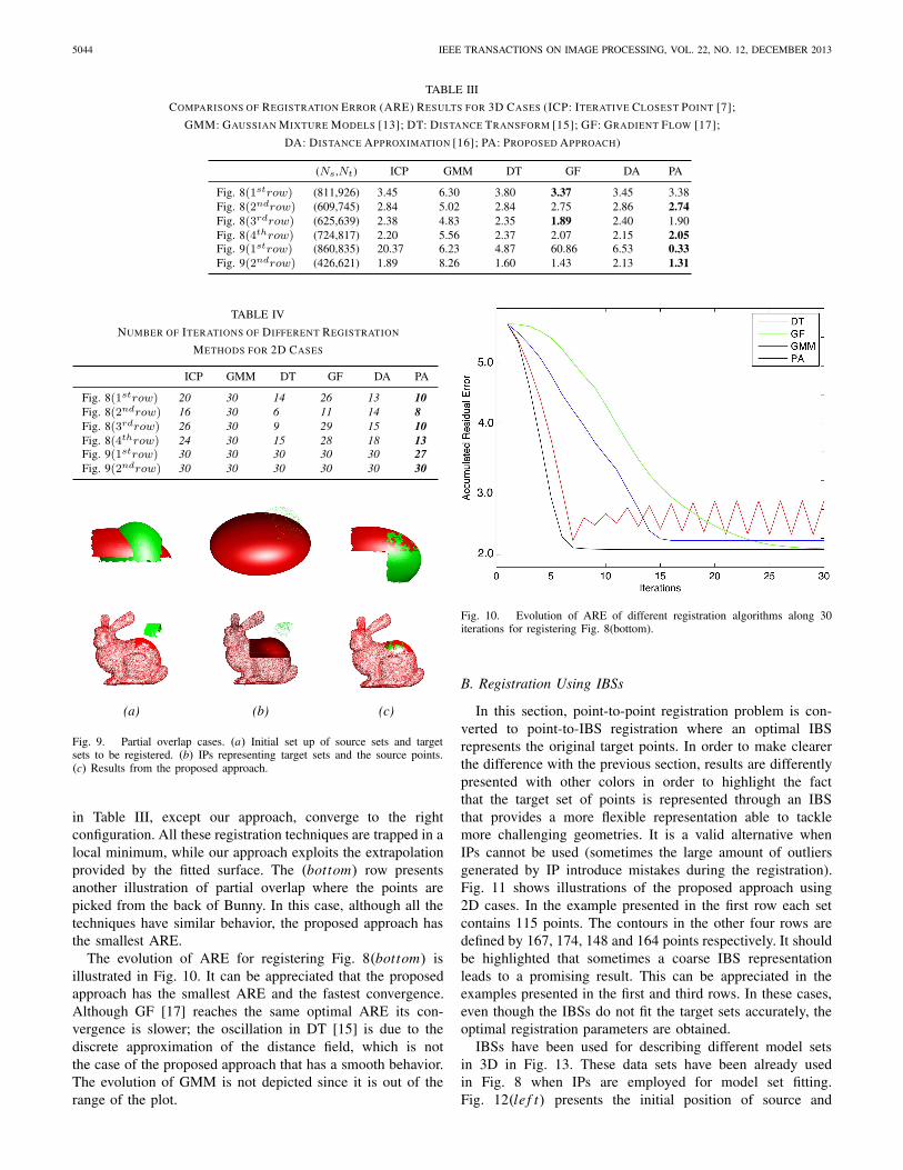
Finally, two cases where the source and target are partiallyoverlapped are presented in Fig. 9. The (top) row shows asimple example where the source and target sets are pickedfrom the same ellipsoid, which is described by a second degreeIP in the presented approach. These two sets are partiallyoverlapped (about 40%) as shown in the last column. Despitethe simplicity of the problem, none of the techniques presented


TABLE III

COMPARISONS OF REGISTRATION ERROR (ARE) RESULTS FOR 3D CASES (ICP: ITERATIVE CLOSEST POINT [7];

GMM: GAUSSIAN MIXTURE MODELS [13]; DT: DISTANCE TRANSFORM [15]; GF: GRADIENT FLOW [17];

DA: DISTANCE APPROXIMATION [16]; PA: PROPOSED APPROACH)

TABLE IV



Fig. 9. Partial overlap cases. (a) Initial set up of source sets and targetsets to be registered. (b) IPs representing target sets and the source points.(c) Results from the proposed approach.

in Table III, except our approach, converge to the rightconfiguration. All these registration techniques are trapped in alocal minimum, while our approach exploits the extrapolationprovided by the fitted surface. The (bottom) row presentsanother illustration of partial overlap where the points arepicked from the back of Bunny. In this case, although all thetechniques have similar behavior, the proposed approach hasthe smallest ARE.

The evolution of ARE for registering Fig. 8(bottom) isillustrated in Fig. 10. It can be appreciated that the proposedapproach has the smallest ARE and the fastest convergence.Although GF [17] reaches the same optimal ARE its con-vergence is slower; the oscillation in DT [15] is due to thediscrete approximation of the distance field, which is notthe case of the proposed approach that has a smooth behavior.The evolution of GMM is not depicted since it is out of therange of the plot.

Fig. 10. Evolution of ARE of different registration algorithms along 30iterations for registering Fig. 8(bottom).

B. Registration Using IBSs

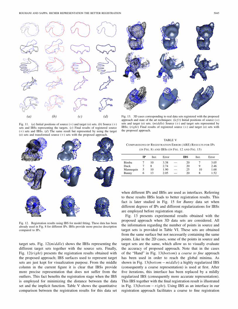
In this section, point-to-point registration problem is con-verted to point-to-IBS registration where an optimal IBSrepresents the original target points. In order to make clearerthe difference with the previous section, results are differentlypresented with other colors in order to highlight the factthat the target set of points is represented through an IBSthat provides a more flexible representation able to tacklemore challenging geometries. It is a valid alternative whenIPs cannot be used (sometimes the large amount of outliersgenerated by IP introduce mistakes during the registration).Fig. 11 shows illustrations of the proposed approach using2D cases. In the example presented in the first row each setcontains 115 points. The contours in the other four rows aredefined by 167, 174, 148 and 164 points respectively. It shouldbe highlighted that sometimes a coarse IBS representationleads to a promising result. This can be appreciated in theexamples presented in the first and third rows. In these cases,even though the IBSs do not fit the target sets accurately, theoptimal registration parameters are obtained.

IBSs have been used for describing different model setsin 3D in Fig. 13. These data sets have been already usedin Fig. 8 when IPs are employed for model set fitting.Fig. 12(le f t) presents the initial position of source and


Fig. 11. (a) Initial positions of source (+) and target (o) sets. (b) Source (+)sets and IBSs representing the targets. (c) Final results of registered source(+) sets and IBSs. (d) The same result but represented by using the target(o) sets and transformed source (+) sets with the proposed approach.

Fig. 12. Registration results using IBS for model fitting. These data has beenalready used in Fig. 8 for different IPs. IBSs provide more precise descriptioncompared to IPs.

target sets. Fig. 12(middle) shows the IBSs representing thedifferent target sets together with the source sets. Finally,Fig. 12(right) presents the registration results obtained withthe proposed approach; IBS surfaces used to represent targetsets are just kept for visualization purpose. From the middlecolumn in the current figure it is clear that IBSs providemore precise representation that does not suffer from theoutliers. This fact benefits the registration stage when the IBSis employed for minimizing the distance between the dataset and the implicit function. Table V shows the quantitativecomparison between the registration results for this data set

Fig. 13. 3D cases corresponding to real data sets registered with the proposedapproach and state of the art techniques: (le f t) Initial positions of source (+)sets and target (o) sets. (middle) Source (+) and target sets represented byIBSs; (right) Final results of registered source (+) and target (o) sets withthe proposed approach.

TABLE V

COMPARISONS OF REGISTRATION ERROR (ARE) RESULTS FOR IPs

(IN FIG. 8) AND IBSs (IN FIG. 12 AND FIG. 15)

when different IPs and IBSs are used as interfaces. Referringto these results IBSs leads to better registration results. Thisfact is later studied in Fig. 15 for Bunny data set whendifferent degrees of IPs and different regularizations for IBSsare employed before registration stage.

Fig. 13 presents experimental results obtained with theproposed approach when 3D data sets are considered. Allthe information regarding the number of points in source andtarget sets is provided in Table VI. These sets are obtainedfrom the same surface but not necessarily containing the samepoints. Like in the 2D cases, some of the points in source andtarget sets are the same, which allow us to visually evaluatethe accuracy of proposed approach. Note that in the casesof the “Hand” in Fig. 13(bottom) a coarse to fine approachhas been used in order to reach the global minima. Asshown in Fig. 13(bottom − middle) a highly regularized IBS(consequently a coarse representation) is used at first. Afterfive iterations, this interface has been replaced by a mildlyregularized IBS (consequently more accurate representation).This IBS together with the final registration result is illustratedin Fig. 13(bottom − right). Using IBS as an interface in ourregistration approach facilitates a coarse to fine registration


TABLE VI

COMPARISONS OF IBS REGISTRATION ERROR (ARE) RESULTS FOR 3D CASES (ICP: ITERATIVE CLOSEST POINT [7]; GMM: GAUSSIAN MIXTURE

MODELS [13]; DT: DISTANCE TRANSFORM [15]; GF: GRADIENT FLOW [17]; DA: DISTANCE APPROXIMATION [16]; PA: PROPOSED APPROACH)

TABLE VII



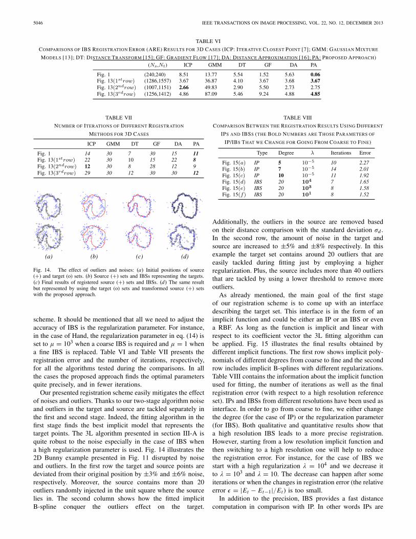
Fig. 14. The effect of outliers and noises: (a) Initial positions of source(+) and target (o) sets. (b) Source (+) sets and IBSs representing the targets.(c) Final results of registered source (+) sets and IBSs. (d) The same resultbut represented by using the target (o) sets and transformed source (+) setswith the proposed approach.

scheme. It should be mentioned that all we need to adjust theaccuracy of IBS is the regularization parameter. For instance,in the case of Hand, the regularization parameter in eq. (14) isset to μ = 103 when a coarse IBS is required and μ = 1 whena fine IBS is replaced. Table VI and Table VII presents theregistration error and the number of iterations, respectively,for all the algorithms tested during the comparisons. In allthe cases the proposed approach finds the optimal parametersquite precisely, and in fewer iterations.

Our presented registration scheme easily mitigates the effectof noises and outliers. Thanks to our two-stage algorithm noiseand outliers in the target and source are tackled separately inthe first and second stage. Indeed, the fitting algorithm in thefirst stage finds the best implicit model that represents thetarget points. The 3L algorithm presented in section III-A isquite robust to the noise especially in the case of IBS whena high regularization parameter is used. Fig. 14 illustrates the2D Bunny example presented in Fig. 11 disrupted by noiseand outliers. In the first row the target and source points aredeviated from their original position by ±3% and ±6% noise,respectively. Moreover, the source contains more than 20outliers randomly injected in the unit square where the sourcelies in. The second column shows how the fitted implicitB-spline conquer the outliers effect on the target.

TABLE VIII

COMPARISON BETWEEN THE REGISTRATION RESULTS USING DIFFERENT

IPS AND IBSS (THE BOLD NUMBERS ARE THOSE PARAMETERS OF

IP/IBS THAT WE CHANGE FOR GOING FROM COARSE TO FINE)

Additionally, the outliers in the source are removed basedon their distance comparison with the standard deviation σd .In the second row, the amount of noise in the target andsource are increased to ±5% and ±8% respectively. In thisexample the target set contains around 20 outliers that areeasily tackled during fitting just by employing a higherregularization. Plus, the source includes more than 40 outliersthat are tackled by using a lower threshold to remove moreoutliers.

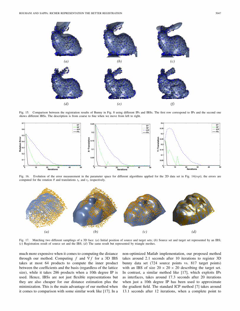
As already mentioned, the main goal of the first stageof our registration scheme is to come up with an interfacedescribing the target set. This interface is in the form of animplicit function and could be either an IP or an IBS or evena RBF. As long as the function is implicit and linear withrespect to its coefficient vector the 3L fitting algorithm canbe applied. Fig. 15 illustrates the final results obtained bydifferent implicit functions. The first row shows implicit poly-nomials of different degrees from coarse to fine and the secondrow includes implicit B-splines with different regularizations.Table VIII contains the information about the implicit functionused for fitting, the number of iterations as well as the finalregistration error (with respect to a high resolution referenceset). IPs and IBSs from different resolutions have been used asinterface. In order to go from coarse to fine, we either changethe degree (for the case of IP) or the regularization parameter(for IBS). Both qualitative and quantitative results show thata high resolution IBS leads to a more precise registration.However, starting from a low resolution implicit function andthen switching to a high resolution one will help to reducethe registration error. For instance, for the case of IBS westart with a high regularization λ = 104 and we decrease itto λ = 103 and λ = 10. The decrease can happen after someiterations or when the changes in registration error (the relativeerror ε = |Et − Et−1|/Et ) is too small.

In addition to the precision, IBS provides a fast distancecomputation in comparison with IP. In other words IPs are


Fig. 15. Comparison between the registration results of Bunny in Fig. 8 using different IPs and IBSs. The first row correspond to IPs and the second oneshows different IBSs. The description is from coarse to fine when we move from left to right.

Fig. 16. Evolution of the error measurement in the parameter space for different algorithms applied for the 2D data set in Fig. 14(top); the errors arecomputed for the rotation θ and translations tx and ty respectively.

Fig. 17. Matching two different samplings of a 3D face: (a) Initial position of source and target sets; (b) Source set and target set represented by an IBS;(c) Registration result of source set and the IBS; (d) The same result but represented by triangle meshes.

much more expensive when it comes to computing the distancethrough our method. Computing f and ∇ f for a 3D IBStakes at most 64 products to compute the inner productbetween the coefficients and the basis (regardless of the latticesize), while it takes 286 products when a 10th degree IP isused. Hence, IBSs are not just flexible representations butthey are also cheaper for our distance estimation plus theminimization. This is the main advantage of our method whenit comes to comparison with some similar work like [17]. In a

non-optimized Matlab implementation, our proposed methodtakes around 2.1 seconds after 10 iterations to register 3Dbunny data set (724 source points vs. 817 target points)with an IBS of size 20 × 20 × 20 describing the target set.In contrast, a similar method like [17], which exploits IPsas interfaces, takes around 17.3 seconds after 20 iterationswhen just a 10th degree IP has been used to approximatethe gradient field. The standard ICP method [7] takes around13.1 seconds after 12 iterations, when a complete point to


point comparison is considered for correspondence search.The quadratic distance in [16] demands 5.5 seconds for 20iterations with a downsampling of 10, but it requires expensivecomputations to estimate the principal curvatures. The methodin [15] is quite fast during registration (less than 1 secondfor 20 iterations) but it highly depends on the distance fieldresolution that requires a lot of computations before startingthe registration.

In all the qualitative comparisons in this manuscript we justpresented the number of iterations as well as the registrationerrors in terms of euclidean distance between the target setand the transformed data set. However, the results could becompared in terms of the transformation parameters. Unfortu-nately, the distance in the parameter space does not lead to afair comparison that is geometrically meaningful. For instance,a translated set that is two units away from the original one hasthe same L1 distance as the one for a transformed set with oneunit translation and rotation, while geometrically can be muchfurther. Fig. 16 illustrates the evolution of the rigid parametersfor the 2D registration problem in Fig. 14(top). The top plot inFig. 16 illustrates the evolution of the rotation parameter whilethe rest two concern the translation along x and y directions.In this typical example ICP shows a slow convergence whileour proposed method converges in first few iterations. As thelast column depicts, ICP seems to diverges during the first fiveiterations, while it is converging in the geometric space. Themethod of discrete distance transform seems to be oscillatingsince it depends on the distance field resolution and it getsstuck and oscillates when it get beyond this resolution.

Fig. 17 shows two different samplings of a 3D face. Bothsource set and target set are sampled from a 3D scanned face.The original point cloud contains more than 112k points, whilethe sampled sets contain 2242 points. We employ an IBS witha lattice of size 203 and a moderate regularization λ = 200.Fig. 17(b) shows how the target set is replaced with the IBS.Then, registration is performed between the source points andthe IBS model. Note that no correspondence search is applied;hence, instead of O(N2

s ) comparisons only O(Ns ) computa-tions for the source set with Ns = 1242 points are applied.In Fig. 17(c) the final alignment between the source and IBSafter 12 iterations is shown. Of course, the aligned source setis not a perfect alignment of IBS, but the final figure illustrateshow it perfectly matches the target set (see Fig. 17(d)).

V. CONCLUSION

In this paper two flexible implicit representations areexploited to tackle the registration problem. In the first stageIPs and IBSs are used to describe a cloud of points. Theoptimal implicit representation is obtained through a linearleast squares formulation; furthermore, in the IBS case, itssmoothness can be easily controlled by the regularizationparameter. In the second stage we exploit the simplicity andflexibility of IPs and IBSs to propose a registration distance.Hence, the point-to-point registration problem is convertedinto a point-to-model one. Then, the registration problemcan be tackled in different stages starting from a coarse tofine representation for the target set. Moreover, the resulting

distance from the implicit function and its gradient informa-tion can be easily computed and it fits the requirement ofany gradient based optimization algorithm to find the bestregistration parameters. Experimental results and comparisonsare provided showing both fast convergence and robustnessin challenging situations. Moreover, it is shown how a coarseto fine representation can lead the convergence to the globaloptimum.

ACKNOWLEDGMENT

The authors would like to thank the Associate Editor andthe anonymous referees for their valuable and constructivecomments.

REFERENCES

[1] Y. Chen and G. Medioni, “Object modelling by registration of multiplerange images,” J. Image Vis. Comput., vol. 10, no. 3, pp. 145–155,1992.

[2] M. Taron, N. Paragios, and M. Jolly, “Registration with uncertaintiesand statistical modeling of shapes with variable metric kernels,” IEEETrans. Pattern Anal. Mach. Intell., vol. 31, no. 1, pp. 99–113, Jan. 2009.

[3] M. Rouhani and A. Sappa, “Non-rigid shape registration: A single lin-ear least squares framework,” in Proc. ECCV, Firenze, Italy, Oct. 2012,pp. 264–277.

[4] M. Rouhani and A. Sappa, “Correspondence free registration througha point-to-model distance minimization,” in Proc. ICCV, Barcelona,Spain, Nov. 2011, pp. 2150–2157.

[5] M. Rouhani and A. Sappa, “Implicit B-spline fitting using the 3Lalgorithm,” in Proc. 18th IEEE ICIP, Sep. 2011, pp. 893–896.

[6] N. Gelfand, N. Mitra, L. Guibas, and H. Pottmann, “Robust globalregistration,” in Proc. Symp. Geometry Process., Vienna, Austria,Jul. 2005, pp. 197–206.

[7] P. Besl and N. McKay, “A method for registration of 3D shapes,”IEEE Trans. Pattern Anal. Mach. Intell., vol. 14, no. 2, pp. 239–256,Feb. 1992.

[8] G. Sharp, S. Lee, and D. Wehe, “ICP registration using invariantfeatures,” IEEE Trans. Pattern Anal. Mach. Intell., vol. 24, no. 1,pp. 90–102, Jan. 2002.

[9] T. Zinßer, J. Schmidt, and H. Niemann, “A refined ICP algorithmfor robust 3D correspondence estimation,” in Proc. ICIP, 2003,pp. 695–698.

[10] J. Ho, A. Peter, A. Rangarajan, and M. Yang, “An algebraic approach toaffine registration of point sets,” in Proc. ICCV, 2009, pp. 1335–1340.

[11] J.-P. Tarel, H. Civi, and D. B. Cooper, “Pose estimation of free-form3D objects without point matching using algebraic surface models,” inProc. IEEE Workshop Model Based 3D Image Anal., Mumbai, India,Jan. 1998, pp. 13–21.

[12] H. Wang, Q. Zhang, B. Luo, and S. Wei, “Robust mixture modellingusing multivariate t-distribution with missing information,” PatternRecognit. Lett., vol. 25, no. 6, pp. 701–710, 2004.

[13] B. Jian and B. Vemuri, “A robust algorithm for point set registrationusing mixture of Gaussians,” in Proc. 10th IEEE ICCV, Oct. 2005,pp. 1246–1251.

[14] F. Boughorbel, M. Mercimek, A. Koschan, and M. Abidi, “A newmethod for the registration of three-dimensional point-sets: TheGaussian fields framework,” Image Vis. Comput., vol. 28, no. 1,pp. 124–137, 2010.

[15] A. Fitzgibbon, “Robust registration of 2D and 3D point sets,” ImageVis. Comput., vol. 21, nos. 13–14, pp. 1145–1153, 2003.

[16] H. Pottmann, S. Leopoldseder, and M. Hofer, “Registration withoutICP,” Comput. Vis. Image Understand., vol. 95, no. 1, pp. 54–71,2004.

[17] B. Zheng, R. Ishikawa, T. Oishi, J. Takamatsu, and K. Ikeuchi, “A fastregistration method using IP and its application to ultrasound imageregistration,” IPSJ Trans. Comput. Vis. Appl., vol. 1, pp. 209–219,Sep. 2009.


[18] M. Blane, Z. Lei, H. Civil, and D. Cooper, “The 3L algorithmfor fitting implicit polynomials curves and surface to data,” IEEETrans. Pattern Anal. Mach. Intell., vol. 22, no. 3, pp. 298–313,Mar. 2000.

[19] H. Dinh, G. Turk, and G. Slabaugh, “Reconstructing surfacesby volumetric regularization using radial basis functions,” IEEETrans. Pattern Anal. Mach. Intell., vol. 24, no. 10, pp. 1358–1371,Oct. 2002.

[20] M. Aigner and B. Juttler, “Gauss-Newton-type technique for robustlyfitting implicit defined curves and surfaces to unorganized data points,”in Proc. IEEE Int. Conf. SMI, Jun. 2008, pp. 121–130.

[21] H. Chui and A. Rangarajan, “A feature registration framework usingmixture models,” in Proc. IEEE Workshop MMBIA, Jun. 2000,pp. 190–197.

[22] B. Zheng, J. Takamatsu, and K. Ikeuchi, “An adaptive and stablemethod for fitting implicit polynomial curves and surfaces,” IEEETrans. Pattern Anal. Mach. Intell., vol. 32, no. 3, pp. 561–568,Mar. 2010.

[23] J. Hermans, D. Smeets, D. Vandermeulen, and P. Suetens, “Robustpoint set registration using EM-ICP with information-theoreticallyoptimal outlier handling,” in Proc. IEEE CVPR, Jun. 2011,pp. 2465–2472.

[24] S. Rusinkiewicz and M. Levoy, “Efficient variants of the ICP algo-rithm,” in Proc. 3rd Int. 3DIM, May/Jun. 2001, pp. 145–152.

[25] G. Taubin, “Estimation of planar curves, surfaces, and nonplanar spacecurves defined by implicit equations with applications to edge andrange image segmentation,” IEEE Trans. Pattern Anal. Mach. Intell.,vol. 13, no. 11, pp. 1115–1138, Nov. 1991.

[26] R. Fletcher, Practical Methods of Optimization. New York, NY, USA:Wiley, 1990.

[27] (2013). AIM@SHAPE, Digital Shape WorkBench [Online]. Available:http://shapes.aimatshape.net/

[28] (2013). The Stanford 3D Scanning Repository [Online]. Available:http://graphics.stanford.edu/data/3Dscanrep/

Mohammad Rouhani (S’09) received the bach-elor’s degree in applied mathematics from theNational University of Iran, Tehran, Iran, in 2003and the master’s degree from the Sharif Univer-sity of Technology, Tehran, Iran, in 2006. Havingexperienced two years of lecturing in Computer Sci-ence, he joined Advanced Driver Assistance SystemsGroup at the Computer Vision Center in Barcelona,Spain, where he received the Ph.D. degree in Com-puter Vision, in 2012. After holding a research posi-tion in Computer Vision and Learning Laboratory at

Imperial College London, London, U.K., he joined Morpheo team at InriaRhone-Alpes, Grenoble, France. His current research interests include 3DComputer Vision and Computer Graphics, including shape modeling, surfacereconstruction, and 3D object registration. He is also currently involved inresearch on machine learning techniques, including randomized decision treesapplied for object detection and 3D pose estimation.

Angel Domingo Sappa (S’94–M’00–SM’12)received the electromechanical engineering degreefrom the National University of La Pampa, GeneralPico, Argentina, in 1995 and the Ph.D. degreein industrial engineering from the PolytechnicUniversity of Catalonia, Barcelona, Spain, in 1999.In 2003, after holding research positions in France,the U.K., and Greece, he was with the ComputerVision Center, where he is currently a SeniorResearcher. He is a member of the Advanced DriverAssistance Systems research group. His current

research interests include a broad spectrum within the 2D and 3D imageprocessing, stereoimage processing and analysis, 3D modeling, dense opticalflow estimation, and visual SLAM for driving assistance.

the richer representation the better registration

Documents