The Reversal of Fortune Thesis Reconsidered∗

Sanghamitra Bandyopadhyay and Elliott Green

Department of Economics and STICERD, University of Birmingham and LSE.

and Development Studies Institute, LSE

The Suntory Centre Suntory and Toyota International Centres for Economics and Related Disciplines London School of Economics and Political Science Houghton Street London WC2A 2AE

EOPP/2010/16 Tel: (020) 7955 6674

∗ We would like to thank Gareth Austin for comments and suggestions, James Robinson for sharing data with us and Frank Brumfit and Erika Macleod for research assistance. All errors, however remain our own.

Abstract

Acemoglu, Johnson, & Robinson (2002) have claimed that the world income distribution underwent a "Reversal of Fortune" from 1500 to the present, whereby formerly rich countries in what is now the developing world became poor while poor ones grew rich. We question their analysis with regard to both of their proxies for pre-modern income, namely urbanization and population density. First, an alternative measure of urbanization with more observations generates a positive (but not significant) correlation between pre-modern and contemporary income. Second, we show that their measure of population density as a proxy is highly flawed inasmuch as it does not properly measure density on arable land, and when corrected with better data the relationship is no longer robust. At best our results demonstrate a Reversal of Fortune only for the four neo-Europes of Australia, Canada, New Zealand and the United States; at worst, we show no Reversal for other former colonies. Keywords: income distribution, population density, Reversal of Fortune,

urbanization. .

This series is published by the Economic Organisation and Public Policy Programme (EOPP) located within the Suntory and Toyota International Centres for Economics and Related Disciplines (STICERD) at the London School of Economics and Political Science. This new series is an amalgamation of the Development Economics Discussion Papers and the Political Economy and Public Policy Discussion Papers. The programme was established in October 1998 as a successor to the Development Economics Research Programme. The work of the programme is mainly in the fields of development economics, public economics and political economy. It is directed by Maitreesh Ghatak. Oriana Bandiera, Robin Burgess, and Andrea Prat serve as co-directors, and associated faculty consist of Timothy Besley, Jean-Paul Faguet, Henrik Kleven, Valentino Larcinese, Gerard Padro i Miquel, Torsten Persson, Nicholas Stern, and Daniel M. Sturm. Further details about the programme and its work can be viewed on our web site at http://sticerd.lse.ac.uk/research/eopp. Our Discussion Paper series is available to download at: http://sticerd.lse.ac.uk/_new/publications/series.asp?prog=EOPP For any other information relating to this series please contact Leila Alberici on: Telephone: UK+20 7955 6674 Fax: UK+20 7955 6951 Email: l.alberici @lse.ac.uk © The authors. All rights reserved. Short sections of text, not to exceed two paragraphs, may be quoted without explicit permission provided that full credit, including © notice, is given to the source.

1 Introduction

In a seminal paper Acemoglu et al. (2002) argue that countries in the devel-oping world have experienced a "Reversal of Fortune," whereby those whichwere previously rich in the pre-colonial era have become poor, while thosethat were poor are now rich. Rather than explaining this reversal throughgeographic factors, they claim that di¤erent sets of institutions imposed bycolonial rule resulted in di¤ering patterns of industrialization over the pasttwo hundred years, and that this phenomenon happened across the colonialworld, regardless of the nature of the colonial power. Their thesis has drawna great deal of attention due to its strong emphasis on European colonialrule as the major explanation for divergence in the modern world incomedistribution.Naturally the biggest problem with any analysis of long-term income

trends is the lack of accurate data on pre-modern income levels. Acemogluet al. (2002) (henceforth AJR) proxy for pre-modern income in two ways,namely urbanization and population density. In both cases they argue that ahigher value represents a higher aggregate income inasmuch as only societieswith high incomes could support urban and dense populations.1

In this paper, however, we question their data for these two proxies of pre-colonial income. First, their measure of urbanization contains no data fromAfrica and thus consists of only 41 observations; when we use an alternativemeasure of urbanization with 71 observations from Africa and the Americasthe relationship disappears and even changes sign. Second, despite theirclaims to the contrary their data on population density does not properlyaccount for arable land, and, when corrected with better data, their resultscollapse across a number of econometric speci�cations. We use standardOrdinary Least Squares regression approaches as done by AJR.We therefore not only suggest that AJR�s analysis does not hold on a

global scale but o¤er two speci�c reasons for this result. First, in no speci-�cations do the data show a reversal within Africa, thereby suggesting thatAfrica�s poverty was largely untouched by colonialism. Secondly, the resultsare largely driven by the four Neo-Europes, which, when excluded, render therelationship between pre-colonial income and contemporary GDP per capitaeither weakly signi�cant or not signi�cant. Thus, while we do not rule out aReversal of Fortune among select countries, our results suggest that whateverreversal took place was not a generalized phenomenon.The rest of the paper is organized as follows. In Section 2, we describe

1Moreover, they are not alone in using these proxies; other recent literature to use oneor both measures include Huillery (2009) and Oster (2004).

1

the di¤erences between AJR�s data on urbanization and population densityand ours. In Section 3 we present our new empirical results of regressingcontemporary income levels on these two proxies of pre-modern incomes. Wethen o¤er an interpretation of the results in Section 4 and Section 5 concludes.

2 Description of the Data

2.1 Urbanization

The �rst proxy used by AJR for income in 1500 is urbanization, or morespeci�cally the percentage of a given population living in cities. They usedata on urbanization from Bairoch (1988) and Eggimann (1999) by sup-plementing Bairoch (1988)�s data on cities greater than 5000 people withEggimann (1999)�s estimates of cities larger than 20,000 people and thenconverting Eggimann (1999)�s data to a 5000-person minimum. They claimin an earlier version that 5000 people is a much better threshold as it ac-counts for a greater number of small pre-modern cities (Acemoglu, Johnson,& Robinson, 2001; Appendix A, p. 1).However, it is no accident that both Chandler (1987) and Eggimann

(1999) only list data on pre-modern cities greater than 20,000 people asthe data on pre-modern urbanization in the developing world is remarkablypoor. Indeed, Bairoch (1988, p. 520) himself notes that "given the currentstate of data and research, it is impossible in the case of most countries toassemble �gures on urban population su¢ ciently complete to give a validindication of the population of all cities with more than �ve thousand;" heindicated that his future e¤orts would be directed at lowering the populationthreshold to 8000 people for Europe.2 Historians agree that data on smallancient cities can be inaccurate for the reasons that abandoned cities candisappear over time, migration routes can make it di¢ cult to measure cities�permanent populations and much archaeological work on ancient cities inthe tropics remains to be done (Connah, 2001; Hopkins, 2009). Thus evenChandler (1987)�s comprehensive data lacks population �gures for 18 of the60 cities he identi�es in Africa and the Americas in 1500.To correct for these problems we use Chandler (1987)�s data on cities

of 20,000 or more for Africa and the Americas. Far from being idiosyn-cratic, the 20,000 benchmark determinant for urbanization is currently usedby such countries as Nigeria and was used for a period by the United Na-

2As acknowledged by Acemoglu et al. (2001, Appendix A, p. 1), Bairoch did notcomplete this work before he died in 1999, let alone move on to completing a dataset ofall pre-modern cities greater than 5000 people.

2

tions; economists and economic historians who have used it as well includeAnnable (1972), Berry (1961), Hoselitz (1957) and Long (2005), among oth-ers. Moreover, using Chandler (1987) as our source has several advantages.First, unlike AJR�s use of both Bairoch (1988) and Eggimann (1999), allof our data originates from a single source. Second, by using data directlyfrom its source we avoid the need to convert it and thereby open ourselvesto criticism of the conversion process.3 Third and �nally, this data allows usto include data on Africa in 1500 in our regressions. While AJR decided toexclude African data because they claim that it was not "detailed" enough(Acemoglu et al., 2002, p. 1238), Chandler (1987)�s data contains 43 citiesin Africa for 1500, or more than twice as many as in the Americas (with 17cities). Moreover, Chandler (1987, p. 6) himself notes that, thanks to 16th-century data on African cities from Leo Africanus, "Africa at 1500 stands asone of the best-prepared lists in this book." While using Chandler (1987)�sdata means that we lose our observations from Asia, where Chandler (1987)only lists cities larger than 40,000, by adding Africa we improve the numberof observations from 41 in AJR to 71 here.

2.2 Population Density

The second proxy used by AJR for pre-modern income is population density.For their data AJR calculate population density on arable land for the simplereason that including non-arable land would make pre-modern states like an-cient Egypt appear very thinly populated and thus not very rich. They taketheir data on arable land from McEvedy & Jones (1978), with the claim thatdoing so "excludes primarily desert, inland water and tundra" (Acemogluet al., 2002, p. 1243). However, while McEvedy & Jones (1978) sometimespresent data on arable land for various countries, in 78 of the 83 observationsused in AJR they list no data on arable land, leading AJR to assume all landas arable for these observations. Yet this assumption is highly problematicin a large number of countries like Australia, Botswana and Canada whichhave large tracts of non-cultivable frozen tundra, deserts and mountains.To correct for this error we employ here data from the FAO (2000), which

for the �rst time estimated global data for land that is potentially arable(or potentially cultivable) for growing any one of twenty-one major cropsunder rainfed conditions, thus making it suitable for assessing populationdensities in 1500 when modern agricultural practices were not yet in use.Much of this potential arable land (henceforth PAL) are currently under

3For instance, AJR use Zipf�s law as one way to convert the data, despite the factthat recent evidence suggests that Zipf�s law does not apply widely across countries (Soo,2005).

3

Country Arable Potential Equivalent PotentialLand Arable Land Arable Land

Canada 100% 12.7% 7.7%Botswana 100 15.8 8.7Australia 100 16.2 10.9

South Africa 100 23 14.7Laos 100 25.4 15.9Kenya 100 26.8 16.6

Rwanda 100 30 19New Zealand 100 32.5 20.1

USA 100 37.5 28.5

Table 1: Selected Discrepancies in Arable Land Measurements, in percent-ages (Source: (Acemoglu et al., 2002; FAO, 2000))

pasture or constitute forests whose clearing would imperil local ecologies,but for simplicity�s sake we assume that all PAL could be cultivated. Wealso examine a more stringent de�nition of PAL called "equivalent potentialarable land" (EPAL) which downgrades marginal land proportional to itssuitability for agriculture.4

We can see the di¤erences between select countries estimated by AJRas having 100% of their land as arable and the FAO data in Table 1. Thedisparities are stark, especially in neo-colonies and Africa. In fact, the FAO�sestimates of PAL may be overly generous in some cases. For instance, theCanada Land Directory grades soil quality from level 1 to level 7, where levels1-4 are suitable for permanent agriculture land, levels 5 and 6 are suitable forgrazing and level 7 is land unsuitable for agriculture; it estimates that only10.3% of Canada�s land falls within levels 1-5, and only 5.0% within levels1-3 (Canada Land Inventory, 1976). Similarly, the Botswanan Ministry ofAgriculture estimated only 5.2% of its land to be cultivable in the 1970s,with only 1% of land under cultivation at any one point (Alverson, 1984).Thus, in at least these two cases, EPAL is a better re�ection of cultivableland than PAL.Another way to assess the accuracy of the FAO data is to compare it to

those cases where McEvedy & Jones (1978) compute arable land for givencountries.5 For instance, AJR calculate only 11.4% of Sudan�s land as cul-

4Where one hectare of very suitable, suitable, moderately suitable and marginal landare counted as 1.0, 0.7, 0.5 and 0.3 hectares, respectively.

5In fact, McEvedy & Jones (1978) do not have a single metric like the FAO for poten-tially arable land; instead they variously list �gures for "cultivated" (Egypt), "productive"

4

tivable based on McEvedy & Jones (1978)�s calculations of arable and pastureland �i.e., land already in some form of use by farmers or pastoralists. Yet,as elsewhere in Africa, Sudan has historically had low population densitiesthat were not able to fully exploit its large tracts of cultivable land. Its largereserves of available fertile land contributed to its reputation in the 1970sas the potential "Breadbasket of the Middle East," which led to subsequentattempts to use land more productively despite ongoing war and poor gov-ernance. Thus the FAO�s calculation of 867,000 Km2 of PAL �or 35% ofall land �is closer to other estimates of 840,000 and 810,000 Km2 from El-Farouk (1996) and Kaikati (1980), respectively, than the mere 300,000 km2calculated by McEvedy & Jones (1978).6

3 Empirical Analysis

With these new data on urbanization and arable land we can now re-estimateAJR�s models. We should note, however, several changes to the dataset.First, eight Caribbean countries included in the AJR paper could not beincluded here due to a lack of data on potential arable land, namely theBahamas, Barbados, Dominica, Grenada, St. Kitts and Nevis, St. Lucia,St. Vincent and Trinidad and Tobago. AJR also lack data on populationdensities for these countries, but assume that they have the same popula-tion density as the Dominican Republic. We could do the same here butsee no reason why we should assume that these countries, which have acombined population of 2.4 million people, had population densities on po-tential arable land in 1500 closer to the Dominican Republic (PAL densityof 3.2) than to Jamaica (32.1). Second, we have also included other formerEuropean colonies with a combined population of 41.5 million people thatwere inexplicably not included in the AJR analysis, namely Cambodia, Dji-bouti, Equatorial Guinea, Guinea-Bissau and Yemen.7 Third, inasmuch asthe "Reversal of Fortune" argument involves the transition from pre-colonialoccupation to colonial domination and then post-colonial independence, weexclude three countries included in AJR which should not have been in theiranalysis, namely Cape Verde (which had no human occupants prior to colo-nialization) and Ethiopia and Nepal (neither of which were colonized by

(Algeria, Morocco and Tunisia), and "pasture" and "arable" (Sudan) land. For more crit-icism of McEvedy & Jones (1978) see Austin (2008b) and Hopkins (2009).

6Sudan�s EPAL is 629,450 Km2, which is still closer to these other estimates than thesum from McEvedy & Jones (1978).

7As with AJR (p. 1244), we exclude from the analysis countries colonized in the 20thcentury for the reason that their colonial experience was too short to have an impact onlong-term economic growth patterns.

5

Europeans). Fourth and �nally, we added countries which were colonized byEuropeans after 1500 and lie in Europe, namely Cyprus (under UK adminis-tration 1878-1960) and Malta (UK administration, 1814-1964). Descriptivestatistics for our variables are presented in Table 9 in the Appendix.We also use three geographical controls in our analysis, namely average

latitude, average distance to coastline and average elevation per country,which are similar to the control variables used by AJR.8

3.1 Urbanization

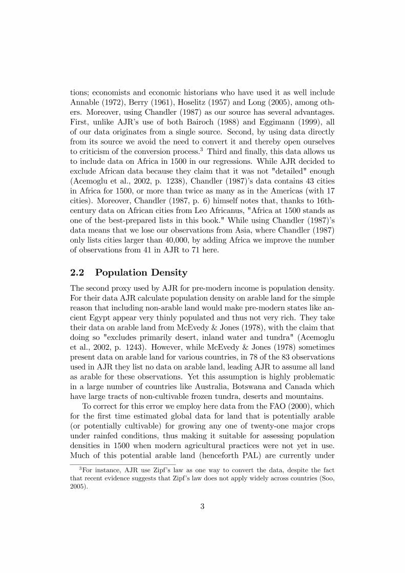
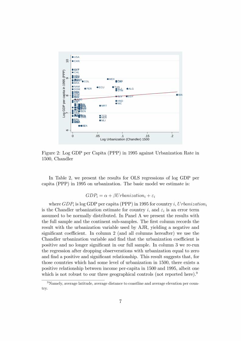
In Figures 1 and 2 we plot log GDP per capita in 1995 against the urbaniza-tion variable used by AJR and our new urbanization variable, CHANDLER,respectively. In Figure 1, the OLS �t suggests a negative relationship be-tween the two variables. However, in Figure 2, the OLS �t suggests a positiverelationship, but the �t is clearly very poor.

ALG

ARG

AUS

BGD

BLZ

BOL

BRA

CAN

CHL

COL CRI

DOMECU

EGYSLV

GTM

GUY

HTI

HND

HKG

IND

IDNJAM

LAO

MYS MEX

MAR

NZL

NICPAK

PAN

PRYPER

PHL

SGP

LKA

TUN

URY

USA

VEN

VNM

67

89

10Lo

g G

DP 

per c

apita

 in 1

995 

(PPP

)

0 5 10 15 20Log Urbanization (AJR) 1500

Figure 1: Log GDP per Capita (PPP) in 1995 against Urbanization Rate in1500, AJR

8We have also used a number of other controls from the literature on long-term economicgrowth patterns (Bockstette et al., 2002; Easterly and Levine, 2003; Olsson and Hibbs,2005; Putterman, 2008), with no changes in our results.

6

ALG

AGO

ARG

BLZ

BEN

BOL

BWABRA

BFA

BUR

CMR

CAN

CAR

TCD

CHL

COL

COD

COG

CRI

CIV

CYP

DJI

DOMECU

EGYSLV

GNQ

ERI

GAB

GMBGHA

GTM

GIN

GNB

GUY

HTI

HND

JAM

KEN

LSO

MDG

MWIMLI

MLT

MRT

MEX

MAR

MOZ

NAM

NIC

NERNGA

PAN

PRYPER

RWA

SEN

SLE

ZAF

SDN

SURSWZ

TZA

TGO

TUN

UGA

URY

USA

VEN

ZMB

ZWE

67

89

10Lo

g G

DP 

per c

apita

 in 1

995 

(PPP

)

0 .05 .1 .15 .2Log Urbanization (Chandler) 1500

Figure 2: Log GDP per Capita (PPP) in 1995 against Urbanization Rate in1500, Chandler

In Table 2, we present the results for OLS regressions of log GDP percapita (PPP) in 1995 on urbanization. The basic model we estimate is:

GDPi = �+ �Urbanizationi + "i

whereGDPi is log GDP per capita (PPP) in 1995 for country i, Urbanizationiis the Chandler urbanization estimate for country i; and "i is an error termassumed to be normally distributed. In Panel A we present the results withthe full sample and the continent sub-samples. The �rst column records theresult with the urbanization variable used by AJR, yielding a negative andsigni�cant coe¢ cient. In column 2 (and all columns hereafter) we use theChandler urbanization variable and �nd that the urbanization coe¢ cient ispositive and no longer signi�cant in our full sample. In column 3 we re-runthe regression after dropping observerations with urbanization equal to zeroand �nd a positive and signi�cant relationship. This result suggests that, forthose countries which had some level of urbanization in 1500, there exists apositive relationship between income per-capita in 1500 and 1995, albeit onewhich is not robust to our three geographical controls (not reported here).9

9Namely, average latitude, average distance to coastline and average elevation per coun-try.

7

When we split the sample by continents, as also done by AJR, we ob-tain di¤erent results for each continent group. We �nd that the relationshipremains signi�cant for the Africa sub-sample (column 4), although this re-sult is not signi�cant upon adding geographical controls (not reported here).Column 5 demonstrates a weakly signi�cant and negative coe¢ cient in thesample excluding Africa; however, as before the coe¢ cient is not signi�cantafter the controls are added (also not reported). We also present results incolumns 6-9 for sub-samples excluding the Neo-Europes (Canada and the USonly, as our data does not include Australia and New Zealand), and for sub-samples of former French, Spanish and British colonies. We obtain a weaklypositive and signi�cant relationship between urbanization and log GDP forthe sample excluding the Neo-Europes, and an insigni�cant relationship in allother sub-samples. We also test for a sub-sample of former British coloniesexcluding the two Neo-Europes (not reported here), with similar results.10

To check to see if we are ignoring smaller cities, we can assume thatthe aforementioned 18 cities listed by Chandler (1987) for Africa and theAmericas that do not have population �gures have the minimum level of20,000 people per city. We rerun our regressions, presented in Panel B; fornone of the sub-samples do we obtain a negative and signi�cant coe¢ cientfor the Urbanization Max variable. The only di¤erences between Panels Aand B are that the sub-sample excluding zero values for urbanization, ourAfrica sub-sample and without Africa sub-sample regressions lose some oftheir signi�cance.

10This sub-sample thus includes such countries as Guyana, India, Jamaica, Kenya andZimbabwe, among others.

8

PanelA:RegressionswithChandlerUrbanizationvariable

Only

Only

Only

Full

Full

Excluding

Only

Without

Without

formerFrench

formerSpanish

formerBritish

AJR

Chandlerzerovalues

Africa

Africa

Neo-Europes

Colonies

Colonies

Colonies

Urbanization

-0.078�

2.121

7.402�

4.222y

-5.660z

3.186z

2.055

-3.739

-1.788

(0.023)

(1.928)

(2.447)(1.834)

(3.199)

(1.873)

(2.580)

(3.619)

(4.533)

R2

0.316

0.008

0.192

0.057

0.091

0.021

0.016

0.065

0.002

N39

7139

4427

6921

1825

PanelB:RegressionswithChandlerUrbanization20,000Maxvariable

Urbanization

1.469

5.957z

3.675z

-4.591

2.095

1.642

-3.523

-2.018

Max

(1.956)

(3.105)(2.018)

(3.113)

(1.929)

(3.016)

(3.610)

(5.036)

R2

0.004

0.064

0.046

0.060

0.009

0.010

0.058

0.009

N71

4044

2769

2118

69Notes

StandarderrorsinparenthesesareWhiteheteroscedasticityrobust.

�:Signi�cantatthe1%

level

y:Signi�cantatthe5%

level

z:Signi�cantatthe10%level

Table2:OLSRegressionsofLogGDPperCapita(PPP)in1995onUrbanization(Chandler)

9

Thus, in using the Chandler de�nition of urbanization we observe thatthe Reversal of Fortune result obtained by AJR does not hold. To summarizeour �ndings:

� The relationship between urbanization and log GDP per capita is notsigni�cant for the (African and American) full sample and all but onesub-sample.

� The relationship is positive and signi�cant for the sub-samples exclud-ing zero values of urbanization and for our Africa sub-sample. However,this result is not robust to the inclusion of geographical controls.

� These results hold whether we include or exclude the 18 cities listed byChandler (1987) that do not have population �gures.

3.2 Population Density

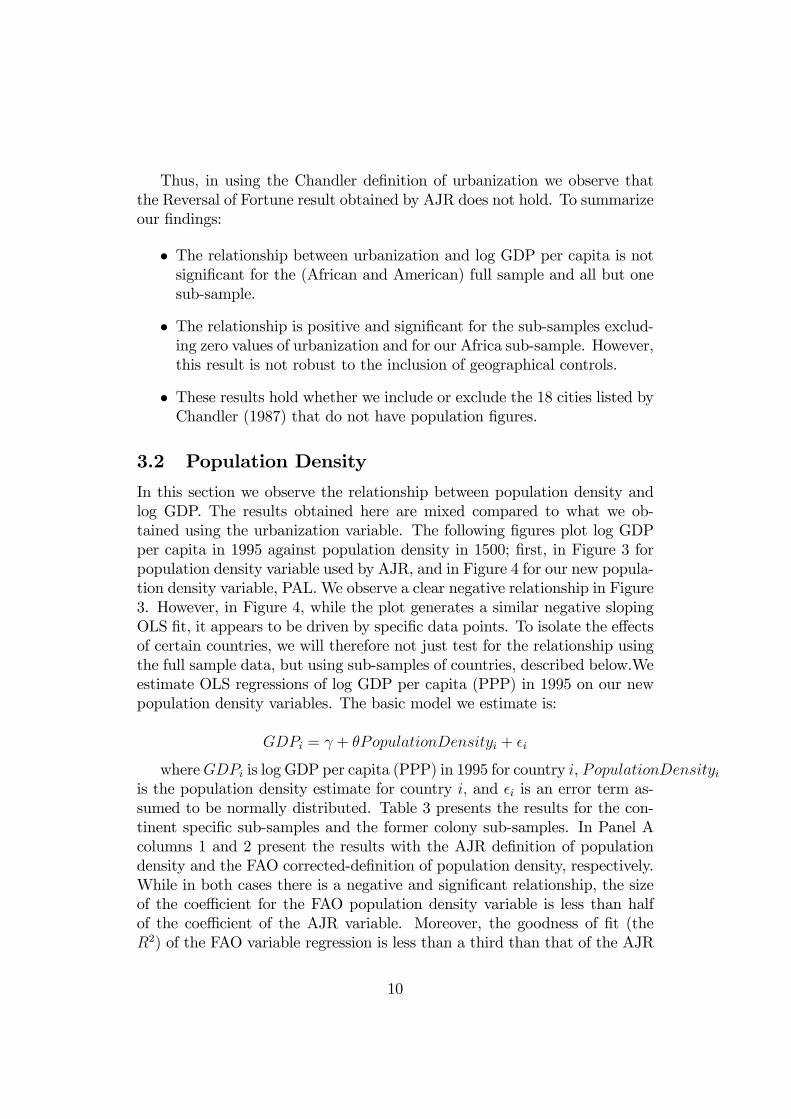
In this section we observe the relationship between population density andlog GDP. The results obtained here are mixed compared to what we ob-tained using the urbanization variable. The following �gures plot log GDPper capita in 1995 against population density in 1500; �rst, in Figure 3 forpopulation density variable used by AJR, and in Figure 4 for our new popula-tion density variable, PAL. We observe a clear negative relationship in Figure3. However, in Figure 4, while the plot generates a similar negative slopingOLS �t, it appears to be driven by speci�c data points. To isolate the e¤ectsof certain countries, we will therefore not just test for the relationship usingthe full sample data, but using sub-samples of countries, described below.Weestimate OLS regressions of log GDP per capita (PPP) in 1995 on our newpopulation density variables. The basic model we estimate is:

GDPi = + �PopulationDensityi + �i

whereGDPi is log GDP per capita (PPP) in 1995 for country i, PopulationDensityiis the population density estimate for country i; and �i is an error term as-sumed to be normally distributed. Table 3 presents the results for the con-tinent speci�c sub-samples and the former colony sub-samples. In Panel Acolumns 1 and 2 present the results with the AJR de�nition of populationdensity and the FAO corrected-de�nition of population density, respectively.While in both cases there is a negative and signi�cant relationship, the sizeof the coe¢ cient for the FAO population density variable is less than halfof the coe¢ cient of the AJR variable. Moreover, the goodness of �t (theR2) of the FAO variable regression is less than a third than that of the AJR

10

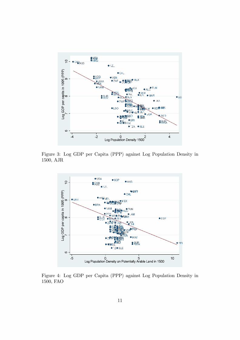
Figure 3: Log GDP per Capita (PPP) against Log Population Density in1500, AJR

Figure 4: Log GDP per Capita (PPP) against Log Population Density in1500, FAO

11

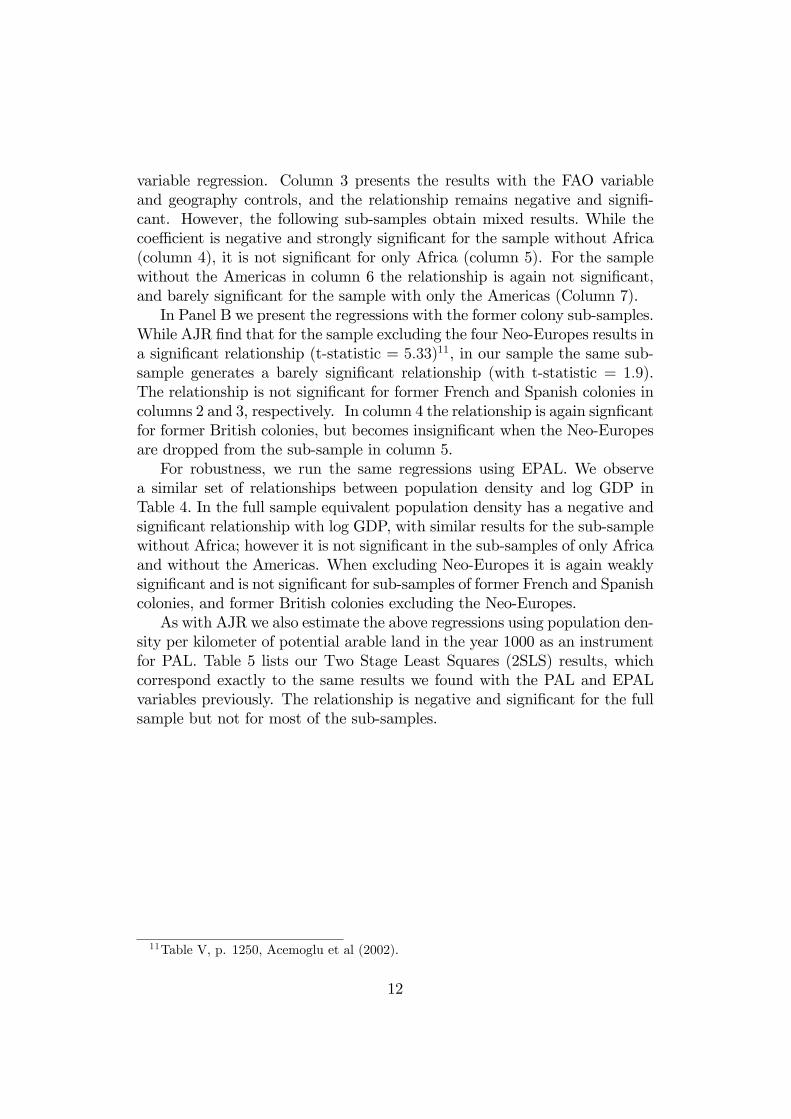
variable regression. Column 3 presents the results with the FAO variableand geography controls, and the relationship remains negative and signi�-cant. However, the following sub-samples obtain mixed results. While thecoe¢ cient is negative and strongly signi�cant for the sample without Africa(column 4), it is not signi�cant for only Africa (column 5). For the samplewithout the Americas in column 6 the relationship is again not signi�cant,and barely signi�cant for the sample with only the Americas (Column 7).In Panel B we present the regressions with the former colony sub-samples.

While AJR �nd that for the sample excluding the four Neo-Europes results ina signi�cant relationship (t-statistic = 5:33)11, in our sample the same sub-sample generates a barely signi�cant relationship (with t-statistic = 1:9).The relationship is not signi�cant for former French and Spanish colonies incolumns 2 and 3, respectively. In column 4 the relationship is again sign�cantfor former British colonies, but becomes insigni�cant when the Neo-Europesare dropped from the sub-sample in column 5.For robustness, we run the same regressions using EPAL. We observe

a similar set of relationships between population density and log GDP inTable 4. In the full sample equivalent population density has a negative andsigni�cant relationship with log GDP, with similar results for the sub-samplewithout Africa; however it is not signi�cant in the sub-samples of only Africaand without the Americas. When excluding Neo-Europes it is again weaklysigni�cant and is not signi�cant for sub-samples of former French and Spanishcolonies, and former British colonies excluding the Neo-Europes.As with AJR we also estimate the above regressions using population den-

sity per kilometer of potential arable land in the year 1000 as an instrumentfor PAL. Table 5 lists our Two Stage Least Squares (2SLS) results, whichcorrespond exactly to the same results we found with the PAL and EPALvariables previously. The relationship is negative and signi�cant for the fullsample but not for most of the sub-samples.

11Table V, p. 1250, Acemoglu et al (2002).

12

PanelA:Regressionsforcontinentsubsamples

Full

Full

Full

Without

Only

Without

Only

AJR

FAO

FAO

Africa

Africa

Americas

Americas

Population

-0.370�

-0.155�

-0.203�

-0.188�

-0.01

-0.075

-0.140z

Density

(0.057)

(0.05)

(0.049)

(0.046)

(0.086)

(0.069)

(0.073)

controls

nono

yes

nono

nono

R2

0.35

0.09

0.29

0.22

0.0

0.02

0.13

N80

8683

4244

6125

PanelB:Regressionsforcolonysubsamples

Without

Onlyformer

Onlyformer

Onlyformer

FormerBritish

Neo-

French

Spanish

British

colonieswithout

Europes

Colonies

Colonies

Colonies

Neo-Europes

Population

-0.087z

-0.233

-0.076

-0.152y

-0.032

Density

(0.046)

(0.258)

(0.064)

(0.064)

(0.069)

controls

nono

nono

noR2

0.03

0.1

0.05

0.1

0.01

N82

2319

3531

Notes

�:Signi�cantatthe1%

level

y:Signi�cantatthe5%

level

z:Signi�cantatthe10%level

Table3:OLSRegressionsofLogGDPperCapita(PPP)in1995onPopulationDensityofPotentialArableLand,

FAO

13

PanelA:Regressionsforcontinentsubsamples

Without

Only

Without

Only

Full

Africa

Africa

Americas

Americas

Population

-0.148�

-0.180�

0.005

-0.067

-0.135z

Density

(0.048)

(0.045)

(0.077)

(0.066)

(0.072)

R2

0.088

0.217

00.017

0.126

N86

4244

6125

PanelB:Regressionsforcolonysubsamples

Without

Only

Only

Only

FormerBritish

Neo-formerFrench

formerSpanish

formerBritish

colonieswithout

Europes

Colonies

Colonies

Europes

Neo-Europes

Population

-0.083z

-0.2

-0.074

-0.144y

-0.029

Density

0.044

0.258

0.062

0.062

0.068

R2

0.031

0.081

0.049

0.093

0.005

N82

2319

3531

Notes

StandarderrorsinparenthesesareWhiteheteroscedasticityrobust.

�:Signi�cantatthe1%

level

y:Signi�cantatthe5%

level

z:Signi�cantatthe10%level

Table4:OLSRegressionsofLogGDPperCapita(PPP)in1995onEquivalentPotentialArableLand

14

PanelA:Regressionsforcontinentsubsamples

Without

Only

Without

Only

Full

Africa

Africa

Americas

Americas

Population

-0.148�

-0.180�

0.005

-0.067

-0.135z

Density

(0.048)

(0.045)

(0.077)

(0.066)

(0.072)

R2

0.088

0.217

00.017

0.126

N86

4244

6125

PanelB:Regressionsforcolonysubsamples

Onlyformer

Onlyformer

Onlyformer

FormerBritish

Without

French

Spanish

British

colonieswithout

Neo-Europes

Colonies

Colonies

Colonies

Neo-Europes

Population

-0.083z

-0.20

-0.074

-0.144y

-0.029

Density

(0.044)

(0.258)

(0.062)

(0.062)

(0.068)

R2

0.031

0.080

0.049

0.093

0.004

N82

2319

3531

Notes

StandarderrorsinparenthesesareWhiteheteroscedasticityrobust.

�:Signi�cantatthe1%

level

y:Signi�cantatthe5%

level

z:Signi�cantatthe10%level

Table5:InstrumentalVariableRegressionsofLogGDPperCapita(PPP)in1995onPotentialArableLand

15

Our results in Tables 3 - 5 thus suggest that the relationship betweenpopulation density in 1500 and contemoprary GDP per capita is not robust.We can now summarise our �ndings:

� The relationship between population density and log GDP per capitais negative and signi�cant for the full sample, the sample excludingAfrica, and the sample with former British colonies.

� It is weakly signi�cant for the sample of the Americas and the sampleexcluding the Neo-Europes.

� It is not signi�cant for the sub-samples of Africa, the sample exclud-ing the Americas and the sub-samples of former French, Spanish, andBritish colonies excluding the Neo-Europes.

� Our results are robust for both the PAL and EPAL variables, and theIV regressions.

4 Interpretation

In using new population density and urbanization data we �nd two con-sistent results. First, the data suggests that the Reversal of Fortune thesisfails to work for African countries, which together comprise a majority of ourand AJR�s sample. This �nding adds to and corresponds with a long liter-ature on Africa which suggests that the continent was already poor beforethe advent of formal colonialism in the late 19th century, whether due to theslave trade (Nunn, 2008), low population densities (Austin, 2008a; Green,2010), malaria (Bhattacharyya, 2009; Bloom & Sachs, 1998) or ethnic di-versity (Birchenall, 2009; Easterly & Levine, 1997), among other possiblefactors. It also corresponds to a recent literature suggesting an ambiguousand sometimes positive e¤ect of colonial rule on development in Africa, es-pecially as regards population growth, height and nutrition (Clapham, 2006;Moradi, 2009). As suggested by (Hopkins, 2009), more work on African eco-nomic history is thus necessary to help tease out the e¤ects of colonialism onlong-term economic growth.

Our second consistent �nding is a lack of a reversal among formerFrench and Spanish colonies, accounting for 49% of the sample. While we canexplain the former case by the fact that 19 of 23 former French colonies werein Africa, only 2 of 19 former Spanish colonies were outside the Americas.12

12Namely, Equatorial Guinea and the Philippines.

16

This disparity among colonial powers is not surprising, however, consider-ing the voluminous literature on the di¤erent e¤ects of colonial powers onpost-colonial economic and political development (Bertocchi & Canova, 2002;Blanton, Mason, & Athow, 2001; Grier, 1999; Lange, Mahoney, & Vom Hau,2006). There is some evidence in our results that this disparity is a result ofthe Neo-Europes, but, as with our results for Africa, this remains a topic forfurther investigation.

5 Conclusion

This paper has questioned the empirical analysis of AJR�s Reversal of For-tune thesis, speci�cally as regards their use of both pre-colonial urbanizationand population density as proxies for pre-modern income. We found in bothcases that alternative and more appropriate measurements of both proxiesfail to generate a robust negative relationship between income in 1500 andcontemporary GDP per capita with appropriate levels of statistical signi�-cance, and in the case of urbanization the coe¢ cient even changes signs tosuggest a positive relationship.With our urbanization data we did not �nd any strong evidence of the Re-

versal thesis for either our full sample of countries or any of our sub-samples.With our population density variables our full sample supported the Reversalthesis but several sub-samples did not, namely those that exclude the Amer-icas and include only African countries, former French and Spanish coloniesand former British colonies without Neo-Europes. At best these results sug-gest that a Reversal took place among certain countries, especially in theNeo-Europes; at worst our results suggest a total lack of a Reversal amongmost countries in our sample.Our point here is not to suggest that the Reversal of Fortune argument is

entirely incorrect. There exists a great deal of evidence to suggest that India,for instance, had higher wages than many parts of western Europe in the16th and 17th centuries, but that over the next three centuries Indian wagesdropped while European wages increased dramatically (Allen, 2005). Otherrecent more qualitative work on the subject has agreed with certain aspectsof the Reversal hypothesis even though it suggests alternative mechanisms(Bayly, 2008; Lange et al., 2006). Our evidence, however, suggests thatthat this Reversal was not a global phenomenon, especially in Africa andamong former French and Spanish colonies. This result is also in line withPrzeworski (2004)�s critique of AJR where he observes a Reversal only forthe four Neo-Europes (or what he calls the "British o¤-shoots"). Certainlyfuture scholars would bene�t from further investigations into the nature of

17

this Reversal and its causes.

References

[1] Acemoglu, D., Johnson, S., & Robinson, J. A. (2001). Reversal of For-tune: Geography and Institutions in the Making of the World IncomeDistribution. NBER Working Paper #8460.

[2] Acemoglu, D., Johnson, S., & Robinson, J. A. (2002). Reversal of For-tune: Geography and Institutions in the Making of the ModernWorld Income Distribution. Quarterly Journal of Economics, 117(4),1231-1294.

[3] Allen, R. C. (2005). Real Wages in Europe and Asia: A First Look atthe Long-Term Patterns. In R. C. Allen, T. Bengtsson & M. Dribe(Eds.), Living Standards in the Past (pp. 111-130). Oxford: OxfordUniversity Press.

[4] Alverson, H. (1984). The Wisdom of Tradition in the Development ofDry-Land Farming: Botswana. Human Organization, 43(1), 1-8.

[5] Annable, J. E. (1972). Internal Migration and Urban Unemploymentin Low-Income Countries: A Problem in Simlutaneous Equations.Oxford Economic Papers, 24(3), 399-412.

[6] Austin, G. (2008a). Resources, Techniques and Strategies South of theSahara: Revising the Factor Endowments Perspective on AfricanEconomic Development, 1500-2000. Economic History Review, 61(3),587-624.

[7] Austin, G. (2008b). The �Reversal of Fortune�Thesis and the Compres-sion of History: Perspectives from African and Comparative Eco-nomic History. Journal of International Development, 20(8), 996-1027.

[8] Bairoch, P. (1988). Cities and Economic Development: From the Dawnof History to the Present. Chicago: University of Chicago Press.

[9] Bayly, C. (2008). Indigenous and Colonial Origins of Comparative Eco-nomic Development: The Case of Colonial India and Africa. PolicyResearch Working Paper #4474, World Bank.

[10] Bernhard, M., Reenock, C., & Nordstrom, T. (2004). The Legacy ofWestern Overseas Colonialism on Democratic Survival. InternationalStudies Quarterly, 48(1), 225-250.

18

[11] Berry, B. J. L. (1961). City Size Distributions and Economic Develop-ment. Economic Development and Cultural Change, 9(4), 573-588.

[12] Bertocchi, G., & Canova, F. (2002). Did Colonization Matter forGrowth? An Empirical Investigation into the Historical Causesof Africa�s Underdevelopment. European Economic Review, 46(10),1851-1871.

[13] Bhattacharyya, S. (2009). Root Causes of African Underdevelopment.Journal of African Economies, 18(5), 745-780.

[14] Birchenall, J. A. (2009). Quantitative Aspects of Africa�s Past EconomicDevelopment. Department of Economics, University of California atSanta Barbara.

[15] Blanton, R., Mason, T. D., & Athow, B. (2001). Colonial Style andPost-Colonial Ethnic Con�ict in Africa. Journal of Peace Research,38(4), 473-492.

[16] Bloom, D. E., & Sachs, J. D. (1998). Geography, Demography and Eco-nomic Growth in Africa. Brookings Journal on Economic Activity,2, 207-295.

[17] Bockstette, V, Chanda, A., & Putterman, L. (2002). States andMarkets:The Advantage of an Early Start. Journal of Economic Growth, 7(4),347-369.

[18] Canada Land Inventory. (1976). Land Capability for Agriculture, Pre-liminary Report. Environment Canada, Lands Directorate.

[19] Chandler, T. (1987). Four Thousand Years of Urban Growth: An His-torical Census. Lewiston, NY: St. David�s University Press.

[20] Clapham, C. (2006). The Political Economy of African PopulationChange. Population and Development Review, 32(Supplement), 96-114.

[21] Connah, G. (2001). African Civilizations: An Archaeological Perspective(2 ed.). Cambridge: Cambridge University Press.

[22] Easterly, W. R., & Levine, R. (1997). Africa�s Growth Tragedy: Policiesand Ethnic Divisions. Quarterly Journal of Economics, 112(4), 1203-1250.

[23] Easterly, W. R., & Levine, R. (2003). Tropics, Germs, and Crops: HowEndowments In�uence Economic Development. Journal of MonetaryEconomics, 50(1), 3-40.

19

[24] Eggimann, G. (1999). La Population des villes des Tiers-Mondes,1500-1950. Geneva: Centre d�histoire economique Internationale del�Universite de Geneve.

[25] El-Farouk, A. E. (1996). Economic and Social Impact of EnvironmentalDegradation in Sudanese Forestry and Agriculture. British Journalof Middle Eastern Studies, 23(2), 167-182.

[26] FAO. (2000). Land Resource Potential and Constraints at Regional andCountry Levels. Rome: Food and Agricultural Organization of theUnited Nations.

[27] Firmin-Sellers, K. (2000). Institutions, Context and Outcomes: Explain-ing French and British Rule in West Africa. Comparative Politics,32(3), 253-272.

[28] Green, E. (2010). Demographic Change and Con�ict in ContemporaryAfrica. In Political Demography: Identity, Con�ict and Institutions,edited by Jack A. Goldstone, Eric Kaufman and Monica Du¤y Toft(New York: Palgrave-Macmillan).

[29] Grier, R. M. (1999). Colonial Legacies and Economic Growth. PublicChoice, 98, 317-335.

[30] Hopkins, A. G. (2009). The New Economic History of Africa. Journal ofAfrican History, 50(2), 155-177.

[31] Hoselitz, B. F. (1957). Urbanization and Economic Growth in Asia.Economic Development and Cultural Change, 6(1), 42-54.

[32] Huillery, E. (2009). History Matters: The Long-Term Impact of Colo-nial Public Investments in French West Africa. American EconomicJournal: Applied Economics, 1(2), 176-215.

[33] Kaikati, J. G. (1980). The Economy of the Sudan: A Potential Bread-basket of the Arab World? International Journal of Middle EastStudies, 11(1), 99-123.

[34] Lange, M., Mahoney, J., & Vom Hau, M. (2006). Colonialism and Devel-opment: A Comparative Analysis of Spanish and British Colonies.American Journal of Sociology, 111(5), 1412-1462.

[35] Long, J. (2005). Rural-Urban Migration and Socioeconomic Mobility inVictorian Britain. Journal of Economic History, 65(1), 1-35.

[36] McEvedy, C., & Jones, R. (1978). Atlas of World Population History.New York: Penguin.

20

[37] Moradi, A. (2009). Towards an Objective Account of Nutrition andHealth in Colonial Kenya: A Study of Stature in African Army Re-cruits and Civilians, 1880-1980. Journal of Economic History, 69(3),719-754.

[38] Nunn, N. (2008). The Long Term E¤ects of Africa�s Slave Trade. Quar-terly Journal of Economics, 123(1), 139-176.

[39] Olsson, O., & Hibbs, D. (2005). Biogeography and Long-Run EconomicDevelopment. European Economic Review, 49(4), 909-938.

[40] Oster, E. (2004). Witchcraft, Weather and Economic Growth in Renais-sance Europe. Journal of Economic Perspectives, 18(1), 215-228.

[41] Przeworski, P. (2004). Geography vs. Institutions Revisited: Were For-tunes Reversed? Mimeo, New York University.

[42] Putterman, L. (2008). Agriculture, Di¤usion and Development: RippleE¤ects of the Neolithic Revolution. Economica, 75(300), 729-748.

[43] Soo, K. T. (2005). Zipf�s Law for Cities: A Cross-Country Investigation.Regional Science and Urban Economics, 35(3), 239-263.

21

Population Population PopulationUrban (%) Urban (%) Density Density Density

Country AJR Chandler AJR PAL EPALAlgeria 14 11.0 7.0 11.7 19.6Angola 0.5 1.5 2.1 3.1

Argentina 0 0.0 0.1 0.3 0.4Australia 0 0.0 0.2 0.2

Bangladesh 8.5 23.7 45.2 55.4Belize 9.2 8.8 1.5 4.4 6.5Benin 1.3 4.2 6.0 8.3Bolivia 10.6 0.0 0.8 1.5 2.0

Botswana 0.0 0.1 1.0 1.7Brazil 0 0.0 0.1 0.2 0.3

Burkina Faso 1.3 4.2 6.0 8.3Burundi 0.0 25.0 57.9 94.3

Cambodia 12.3 16.3Cameroon 0.5 1.5 2.1 3.1Canada 0 0.0 0.0 0.2 0.3CAR 0.5 1.5 2.1 3.1Chad 5.5 1.0 4.2 6.3Chile 0 0.0 0.8 18.0 30.0

Colombia 7.9 2.0 1.0 1.5 2.1Congo D. R. 0.5 1.5 2.1 3.1Congo Rep. 0.5 1.5 2.1 3.1Costa Rica 9.2 8.8 1.5 4.4 6.5

Cote d�Ivoire 1.3 4.2 6.0 8.3Cyprus 0.0 46.2 79.4Djibouti 0.0 33.6 78.7

Dominican Rep. 3 0.0 1.5 3.2 4.9Ecuador 10.6 5.0 2.2 4.7 6.5Egypt 14.6 10.9 100.5 3305.8 6779.7

El Salvador 9.2 8.8 1.5 4.4 6.5Eq. Guinea 0.5 2.1 3.1

Eritrea 0.0 2.0 4.6 6.8Gabon 0.5 1.5 2.1 3.1Gambia 1.3 4.2 6.0 8.3Ghana 1.3 4.2 6.0 8.3

Guatemala 9.2 8.8 1.5 4.4 6.5Guinea 1.3 4.2 6.0 8.3

Guinea-Bissau 1.3 4.2 6.0 8.3Guyana 0 0.0 0.2 0.3 0.5

Table 6: Appendix A: Urbanization and Population Density in 150022

Population Population PopulationUrban (%) Urban (%) Density Density Density

Country AJR Chandler AJR PAL EPALHaiti 3 0.0 1.3 3.5 5.9

Honduras 9.2 8.8 1.5 4.4 6.5Hong Kong 3 0.1 20.8 29.4

India 8.5 23.7 45.2 55.4Indonesia 7.3 4.3 10.9 15.7Jamaica 3 0.0 4.6 32.1 46.3Kenya 0.0 2.6 9.5 15.3Laos 7.3 1.7 6.8 10.9

Lesotho 0.0 0.5 2.1 3.2Madagascar 0.0 1.2 2.0 3.1

Malawi 0.0 0.8 1.1 1.7Malaysia 7.3 1.2 3.0 4.2

Mali 5.5 1.0 4.2 6.3Malta 0.0 51.3 76.9

Mauritania 5.5 3.0 4.2 6.3Mexico 14.8 7.1 2.6 9.6 13.7Morocco 17.8 21.0 9.1 12.2 19.6

Mozambique 0.0 1.3 1.6 2.3Namibia 0.0 0.1 1.0 1.7

New Zealand 3 0.4 0.6 0.9Nicaragua 9.2 8.8 1.5 4.4 6.5

Niger 5.5 1.0 4.2 6.3Nigeria 1.3 4.2 6.0 8.3Pakistan 8.5 23.7 45.2 55.4Panama 9.2 8.8 1.5 4.4 6.5Paraguay 0 0.0 0.5 0.9 1.5

Peru 10.5 2.5 1.6 4.6 6.5Philippines 3 1.7 5.4 7.4Rwanda 0.0 25.0 57.9 94.3Senegal 1.3 4.2 6.0 8.3

Sierra Leone 1.3 4.2 6.0 8.3Singapore 3 0.1 3.0 4.2

South Africa 0.0 0.5 2.1 3.2Sri Lanka 8.5 15.5 26.9 32.4Sudan 0.5 14.0 4.6 6.4

Suriname 0.0 0.2 0.3 0.5Swaziland 0.0 0.5 2.1 3.2Tanzania 1.7 2.0 2.6 3.8

Table 7: Appendix A: Urbanization and Population Density in 1500, contin-ued

23

Population Population PopulationUrban (%) Urban (%) Density Density Density

Country AJR Chandler AJR PAL EPALTogo 1.3 4.2 6.0 8.3

Tunisia 12.3 8.1 11.7 24.2 38.6Uganda 0.0 7.5 10.6 15.3Uruguay 0 0.0 0.1 0.0 0.0

USA 0 0.0 0.1 0.2 0.3Venezuela 0 0.0 0.4 0.7 1.0Vietnam 7.3 6.1 17.3 25.6Yemen 45000.0 112500.0Zambia 0.0 0.8 1.1 1.7

Zimbabwe 0.0 0.8 1.1 1.7

Table 8: Appendix A: Urbanization and Population Density in 1500, contin-ued

24

ObservationsMeanValue

StandardDeviation

Minimum

Maximum

LogofGDPpercapita(PPP)in1995

867.87

1.01

6.25

10.22

Populationdensityin1500onpotential

87575.86

4832.19

0.01

45000

arableland(PAL)

Populationdensityin1500onequivalentpotential

941281.93

11615.62

0.01

112500

arableland(EPAL)

Logofpopulationdensityin1500(PAL)

871.52

1.97

-4.96

10.71

Logofpopulationdensityin1500(EPAL)

941.85

1.95

-4.83

11.63

Urbanizationin1500(Chandler)

720.024

0.039

0.000

0.210

Urbanization(Chandler),maximum

value

720.027

0.040

0.000

0.210

Table9:AppendixB:DescriptiveStatisticsofKeyVariables

25