the return of zipf: towards a further understanding … jrs 1999.p… · why do cities exist, and...

THE RETURN OF ZIPF: TOWARDS A FURTHERUNDERSTANDING OF THE RANK-SIZE DISTRIBUTION*

Steven BrakmanUniversity of Groningen, Department of Economics, P.O. Box 800, 9700 AV Groningen,The Netherlands. E-mail: [email protected]

Harry GarretsenUniversity of Nijmegen, Department of Economics, P.O. Box 9108, 6500 HK, Nijmegen,The Netherlands. E-mail: [email protected]

Charles Van MarrewijkErasmus University Rotterdam, P.O. Box 1738, 3000 DR, Rotterdam, The Netherlands.E-mail: [email protected]

Marianne van den BergUniversity of Groningen, Department of Economics, P.O. Box 800, 9700 AV, Groningen,The Netherlands. E-mail: [email protected]

ABSTRACT. We offer a general-equilibrium economic approach to Zipf ’s Law or, moregenerally, the rank-size distribution—the striking empirical regularity concerning the sizedistribution of cities. We provide some further understanding of Zipf ’s Law by incorporat-ing negative feedbacks (congestion) in a popular model of economic geography andinternational trade. This model allows the powers of agglomeration and spreading to bein long-run equilibrium, which enhances our understanding of the existence of a rank-sizedistribution of cities.

1. INTRODUCTION

Why do cities exist, and why do they vary in size? These fundamentalquestions have received a considerable amount of attention from regional andurban economists in recent years. Consequently, a large and growing body ofliterature exists today in which many factors contributing to our understandingof the role, existence, and growth of cities are examined. Cities are now thoughtto arise, for example, to give consumers easy access to a large variety of goods

*We would like to thank three anonymous referees, conference participants at the 1996 WEAmeeting in San Francisco, The Royal Economic Society 1997 in Stoke-on-Trent, the 1997 EEAconference in Toulouse, Monash University, Australia, the University of Osnabrueck, Germany,Andrew Bernard, Catrinus Jepma, Hans Kuiper, Jan Oosterhaven, Teun Schmidt, Dirk Stelder andTom Wansbeek for useful suggestions.

Received May 1997; revised October 1997; accepted November 1997.

© Blackwell Publishers 1999.Blackwell Publishers, 350 Main Street, Malden, MA 02148, USA and 108 Cowley Road, Oxford, OX4 1JF, UK.

JOURNAL OF REGIONAL SCIENCE, VOL. 39, NO. 1, 1999, pp. 183–213

(either public or private), or because of the “external” effects (such as closenessto friends and relatives) of consumer location, or because of the advantage forconsumers of proximity to their workplace (Fujita, 1989). However, consumerswho live and work in cities are also confronted with competition for space,environmental problems, etc. The trade-off between the pros and cons of citiesdetermines the location choice of consumers. The existence of spillovers may alsoplay a role in their location decision of the producers. Cities provide firms witha large clientele, an efficient location for knowledge spillovers or technologicalexternalities, maintenance services, financial services, and legal aid (Fujita andThisse, 1996; Glaeser et al., 1992; Henderson, 1977). Political systems can alsobe important in the formation of cities; Ades and Glaeser argue that an urbangiant may “ultimately stem from the concentration of power in the hands of asmall cadre of agents living in the capital,” (1997, p. 224).

The factors above are no doubt important but they only give a rationale forthe existence of single cities. In general, they do not explain why cities are spreadunevenly across space nor do they explain why systems of cities exist. However,the latter is studied in Central Place Theory (Christaller, 1933; Lösch, 1940;Stewart, 1948; Henderson, 1974; Eaton and Lipsey, 1982; Fujita, Ogawa, andThisse,1988;Abdel-Rahman and Fujita,1993;Abdel-Rahman,1994;Quinzii andThisse, 1990; see Mulligan, 1984, for a survey). For a long time it proved difficultto provide a sound economic rationale for systems of cities. It was up to Eatonand Lipsey (1982) to develop a model with multipurpose shopping that createsa demand externality causing clustering. It remained analytically difficult todetermine the optimal geographic pattern of agglomeration,so Eaton and Lipseyverified whether the equilibrium is consistent with a central place structure.Such hierarchical systems can be shown to be socially optimal given somespecific conditions (Quinzii and Thisse, 1990; Suh, 1991). Subsequent researchshowed that systems of cities may also evolve due to differences in fixed costsor variations in industrial structure, that is, specialization versus diversification(Abdel-Rahman and Fujita, 1993; Abdel-Rahman, 1994) or differences in thetype of goods produced, that is, substitutability (Fujita, Ogawa, and Thisse,1988).

Although the aforementioned studies have clearly contributed to our un-derstanding of systems of cities “it is fair to say that the microeconomicunderpinnings of central place theory are still to be developed,” (Fujita andThisse, 1996, p. 343). Sometimes the hierarchical structure is assumed before-hand, and the purpose of the study is to show that such a system is “optimal” oran “equilibrium” outcome in some sense. Sometimes there is no interactionbetween location decisions, market structure, and price-setting behavior todetermine the evolution of the system of cities. In particular this state of ourtheoretical knowledge about the size-distribution of cities is not very satisfyingbecause we still do not have a proper understanding of the outstanding empiricalregularity concerning city-size distributions: the so-called rank-size distribu-tion.The rank-size distribution states that there is an inverse linear relationship

© Blackwell Publishers 1999.

184 JOURNAL OF REGIONAL SCIENCE, VOL. 39, NO. 1, 1999

between the logarithmic size of a city and its logarithmic rank. A special case ofthe rank-size distribution is known as Zipf ’s Law. Even though the rank-sizedistribution does not hold exactly in reality, it does perform surprisingly well forthe (historical) size distribution of cities in most industrialized countries. None-theless, a convincing theoretic microeconomic foundation for its existence is stilllacking, so it seems that the rank-size distribution is an empirical regularity insearch of a theory in which it can be grounded on the behavior of the individualconsumers and producers.1 As Mulligan put it “At this scale of analysis, researchemphasizes the behavior of the central place system, rather than the motivationsand actions of economic agents,” (1984, p. 25).

Zipf ’s Law can be derived from a stochastic or self-organizational approach,sometimes borrowed from physics (Simon, 1955; Read, 1988; Bura et al., 1996;Krugman, 1996a, 1996b; Roehner, 1995). Haag and Max (1995) explicitly intro-duced “push” and “pull” factors, which are, however, simply assumed to exist andnot derived from microeconomic principles. Eaton and Eckstein (1997) furtherextended this approach by identifying the push and pull factors, for example,distance and human capital. The purpose of this paper is to show how therank-size distribution can be derived from a general-equilibrium economicmodel based on microeconomic principles. The model we use is developed inBrakman et al. (1996). It incorporates negative feedbacks (congestion) in Krug-man’s (1991a, 1991b) geography model. The presence of negative feedbacksexplains the simultaneous existence of large and small cities. This is crucialbecause the rank-size distribution only makes sense in a world in which citiesof various sizes coexist. We show that the model can generate a size distributionof cities that meets the requirements of the rank-size distribution.

The paper is organized as follows. In Section 2 we describe the rank-sizedistribution and discuss the influence of some economic variables on the sizedistribution of cities using The Netherlands as an example. In Section 3 weintroduce the model and show how changes in parameters, such as transporta-tion costs, the degree of industrial activity, returns to scale or congestion costs,influence the rank-size distribution. In Sections 4 and 5 we investigate somestructural aspects of the model and summarize our conclusions.

2. THE RANK-SIZE DISTRIBUTION

Although there seems to be some confusion in the use of terminology (seeRead, 1988, for a short survey of the literature) Zipf ’s Law (Zipf, 1949) wasinitially stated as in Equation (1), in which Rj is the rank of city j, Mj is its size,

1In other words “taking an even longer view the growth of cities in increasingly integratedmarkets raises another intriguing possibility. In the US, cities follow the so-called rank-size rule . . .No one knows quite why this is,” (The Economist, Survey of Cities, July 29th 1995, p. 18).Furthermore, there is a fractal aspect to the rank-size distribution as it also applies at differentlevels of aggregation.


BRAKMAN ET AL.: THE RETURN OF ZIPF 185

and Co is a constant. This elementary version can be generalized (as suggestedby Zipf) to Equation (2), in which q is a (positive) constant.2

(1) RjMj = Co ; j = 1,..,r

(2) Mj = Co

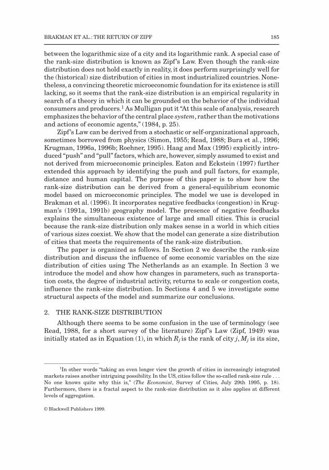
Henceforth we refer to Equation (1) as Zipf ’s Law and Equation (2) as therank-size distribution. Thus, using this terminology Zipf ’s Law is a special caseof the rank-size distribution with the parameter q, which plays an importantrole in the sequel, equal to one.3 The size of each city is measured by itspopulation, and the city with the largest population is given rank 1, thesecond-largest city rank 2, and so on. Under Zipf ’s Law (q=1) the largest city isprecisely k times as large as the kth largest city; the graph of Equation (1) is arectangular hyperbola. In empirical tests the log-linear version of Equation (2)is estimated

(3) log(Mj) = log(Co) – q log(Rj)

Under Zipf ’s Law q = 1 and Figure 1 results. If 0 < q < 1 the slope of thecurve would be flatter and a more even distribution of city sizes results thanpredicted by Zipf ’s Law. If q > 1 large cities are larger than Zipf ’s Law predicts,resulting in a wider dispersion of city sizes.

In general the various estimations of the rank-size distribution for thecity-size distribution of individual countries fit the data remarkably well (seeRead, 1988). The following critical remarks are worth mentioning.

First, the rank variable is a transformation of the size variable, whichinevitably creates a (negative) correlation between the two variables.

Second, a distribution pattern as predicted by the rank-size distribution isoften found only when very small cities are excluded from the sample. If the sizeof the city drops below a certain level (which is neither constant through timenor the same for every country) there is hardly any negative correlation betweensize and rank left for this group of small cities. For instance, Krugman arguesthat the rank-size distribution works best for US cities “over a range of twoorders of magnitude from cities of around 200,000 up to metropolitan New York,with almost 20,000,000” (1996a, p. 95). A possible rationale for this procedure isthat very small cities are indistinguishable from rural areas and can be omittedfrom the data. In other word, there is a threshold value for urbanization, see

Rjq

2Equation (2) is the Lotka form, see Parr (1985) or Roehner (1995). These authors also showthat the problem has been considered prior to Zipf ’s contribution, for example by Auerbach (1913),Goodrich (1925), and Lotka (1925).

3As pointed out by an anonymous referee ‘rank-size rule’ or ‘Zipf ’s Law’ is now standard usageif q = 1, whereas ‘rank-size function’ or ‘rank-size distribution’ is used if q may differ from unity.



FIGURE 1: Rank-Size Rules for The Netherlands.



Roehner (1995) for a discussion. Various methods are used to determine thisthreshold (Parr, 1985).

Third, for the city-size distribution in some countries (notably the USA atpresent) Zipf ’s Law holds because q is not statistically different from 1. However,for most other countries and at different times, q is often found to be differentfrom 1. Therefore unnecessary attention to the value q = 1, is unwarranted (seeKrugman (1996b).

Fourth and most importantly, Equation (2) does not deal with the compara-tive static effects of Zipf ’s Law. The value of q in Equation (2) is not constant overtime.That is,urban growth is not proportional.Sometimes, the urban populationbecomes more concentrated in the larger cities (which increases q) whereasduring other periods the urban population becomes more evenly distributedacross the various cities (which decreases q).4 We now illustrate this point.

A Brief Look at Urbanization and Economic Change

What causes cities to become larger or smaller relative to one another, orwhat accounts for changes in q over time? If one believes, as we do, that thereason for these changes is not necessarily to be found in random growth, butinstead in structural economic changes,a model that links these changes to Zipf ’sLaw is called for. This is the topic of the next section. Parr (1985) investigatesthe size-distribution of cities for various countries since about 1900 and arguesthat over time a nation tends to display an n-shaped pattern in the degree ofinterurban concentration.5 This also holds for The Netherlands, one of theearliest intensively urbanized countries in Europe, which we use as an illustra-tion. The discussion is based on Kooij (1988), who distinguishes three stylizedperiods:6

1. Pre-industrialization (ca. 1600–1850) characterized by high transportationcosts and production dominated by immobile farmers.

2.Industrialization (ca.1850–1900) characterized by declining transportationcosts and the increasing importance of “footloose” industrial productionwith increasing returns to scale.

3. Post-industrialization (ca. 1900–present) characterized by a declining im-portance of industrial production and an increased importance of negativefeedbacks such as congestion.

As early as 1600 The Netherlands contained 20 cities with more than 10,000inhabitants. In terms of the rank-size distribution the size distribution of these

4It must also be emphasized that the ranking of individual cities is not constant over time.The history of urban development is very much a story of the rise and fall of particular cities.

5Parr (1985) finds a U-shaped pattern for the variable 1/q, which therefore translates into ann-shaped pattern for q.

6De Vries (1981, pp. 96–104; 1984) gives additional supporting historical data on Europe asa whole.



cities was relatively even. There was no integrated urban system at the nationallevel until halfway through the nineteenth century, which marks the start of theera of industrialization in The Netherlands. Apart from the fact that theindustrialization process had by and large yet to begin, the relatively hightransportation costs between cities is thought to have provided an additionalimportant economic reason for the lack of a truly national urban system.

The estimation of Equation (3) for The Netherlands reveals that q increasesfrom 0.55 in 1600 to 1.03 in 1900 (per our own calculations, see also Figure 1).7

In the second half of the nineteenth century an integrated urban system wasformed. Two interdependent economic changes were mainly responsible for thisformation. First, the development of canals, a railroad network, and, to a lesserextent, roads significantly lowered transportation costs between cities whichenhanced trade between cities. Second, due to lower transportation costs, theindustrialization process really took off and cities often became more specializedwhich stimulated trade between cities. Although the industrialization processdid not lead to dramatic changes in the overall rank-size order, it can beconcluded nevertheless that as time went by the initially large cities gained arelatively larger share of the urban population.

Structural changes in the rank-size distribution take decades to material-ize, so it is only well into the twentieth century that most Western industrializedcountries, including The Netherlands, gradually entered the post-industrializa-tion era. The share of the services sector in total employment becomes ever moreimportant at the expense of the industrial sector.Comparing the Dutch rank-sizedistribution for 1900 with 1990 it is evident that the size distribution of citieshas become more “flat.” In 1900 q was 1 compared to 0.7 in 1990. The decliningimportance of industry (and hence of production characterized by increasingreturns to scale) may be one factor contributing to this change in the sizedistribution. Increased congestion, especially in the large cities, is thought tohave stimulated the decline of such cities as Amsterdam, Rotterdam, and TheHague.

From the above discussion we conclude that Period 2, the industrializationperiod, was special in its power of agglomeration, as also noted by Kooij “. . thiswas the era of the large cities,” (1988, p. 363). However, for all three periods therank-size distribution holds. This is illustrated in Figure 1 which shows theresults of estimating Equation (3) for our sample of Dutch cities in 1600, 1900,and 1990: at least 96 percent of the variance in city size is explained by therank-size distribution. Industrialization apparently leads to an increase of q andit is during this period (around 1900) that the Dutch rank-size distributionmimics Zipf ’s Law (q = 1). Finally, these three periods in which changes ineconomic variables demonstrably have an impact on the rank-size distributionenable us to simulate the impact of such changes in the sequel of the paper.

7Standard errors are 0.026 and 0.042 and R2s are 0.96 and 0.96, respectively. The sampleconsisted of 19 cities for 1600 and 23 cities for 1900.



3. A GENERAL EQUILIBRIUM MODEL OF INDUSTRIAL LOCATIONAND ZIPF’S LAW

The Model

In Brakman et al. (1996) we extend Krugman’s (1991a, 1991b) generalequilibrium location model. Krugman’s basic location model usually producesonly a few industrial cities of equal size,or even monocentric (one city) industrialproduction, and it is therefore not suited to derive the rank-size distribution.The extension we offer is the possibility of negative feedbacks or negativeexternalities.8 By doing so we can explain the viability of small cities or smallindustrial clusters and thus in principle are able to derive rank-size distribu-tions.

There are N cities producing manufactured goods that consist of manyindividual varieties, nj in city j, and a homogeneous agricultural good, whichserves as numeraire. The production of manufactured goods is characterized byfirm-specific increasing returns to scale, and is assumed to be of the so-called“footloose” type: firms are able to change their production location without costs.The increasing (internal) returns to scale are responsible for the fact that eachvariety is only produced by a single firm. Concentration of production reinforcesfurther concentration because total city income grows if workers decide to moveto that specific city. This pecuniary externality or growth of city income thenattracts more industrial firms and so on. Agricultural production is not mobile,is characterized by perfect competition and, for simplicity, zero transport costs.9

The existence of a local, immobile labor force is an important spreading factorbecause it ensures that there is always a positive demand in each region. If allindustrial production is concentrated in just one location a firm may stillconsider relocation to another city in the hope of gaining a large part of thatcity’s local market by not having to charge transportation costs.

On the demand side it is assumed that each city spends a fixed amount ofits income on both types of goods. This is the outcome of the well-known nestedCobb-Douglas or CES utility function given in Equations (4) and (5), where α isthe share of income spent on manufactured goods and σ is the elasticity ofsubstitution between different varieties of manufactured goods. If we let γ denotethe share of industrial workers in the total work force and λj the share of thesein city j, then the total number of industrial workers in city j, Lj, is given inEquation (6). Finally, let QAj denote production of agricultural goods in city j andφj the share of agricultural workers in city j, then normalization of the productionof agricultural goods, which takes place under constant returns to scale, leadsto Equation (7)

8The properties of this model and a complete description can be found in Brakman et al. (1996).9Positive transport costs for the agricultural sector are investigated in Fujita and Krugman

(1995).



(4) U =

(5) Cm =

(6) Lj = λjγ L

(7) Qaj = φj(1 – γ )L

To analyze location aspects, positive transportation costs of the “iceberg”type are introduced in the manufacturing sector. That is, if one unit of manufac-tured goods is shipped from city j to i only 0 < tij < 1 units arrive in city i. Anincrease in the parameter tij implies a reduction in transport costs from city j tocity i.

It is important in this model that industrial workers (and hence theassociated demand for manufactured products) are located where the productionof manufactured products is located, and vice versa. The agglomeration processis fueled by the interaction of increasing returns, transportation costs, and themobility of the industrial workers. Increasing returns are responsible for indus-trial concentration. However, the fact that some factors of production areimmobile provides for the spreading forces in the model: there is always demandfor manufactures in the periphery, that is in the rural areas.

So far the model is simply a summary of Krugman (1991a, 1991b). Ourmodel differs from his because of the role of negative feedbacks, externaldiseconomies, or congestion costs. These costs provide an additional spreadingforce and thereby enable an equilibrium outcome with not only a few cities, buta reasonable number of cities of different sizes—a necessary condition for atheoretical foundation of Zipf ’s Law. The importance of negative feedbacks wasnoted by Balassa (1961, pp. 202–204); although economies of scale tend toconcentrate production in centrally located cities, there can still be a “spreading”effect towards rural cities. In modern times external diseconomies may arisebecause of limited physical space, limited local resources (such as water forcooling processes), environmental pollution (which may require extra invest-ment), and other congestion effects such as heavy usage of roads, communicationchannels, and storage facilities.

Our aim is to analyze the consequences of congestion rather than its origin.We capture the essence of negative feedbacks in Equation (8), where lij repre-sents the amount of labor necessary to produce xij units of a particular varietyi in city j

(8) lij = fj(nj) + βj (nj)xij ; with , βj ≥ 0

Note that, in contrast to the more commonly used formulation in imperfectcompetition models, the fixed costs (fj) and the variable costs (ßj) depend

C Cm aα α1−

cijj

N

i

nj1 1

1

1−

=

−

∑∑L

NMM

O

QPP

σ

σσ

f j '



positively on the number of firms in the city of location (nj).10 Although a novelfeature in this type of model, Mulligan (1984, pp. 22-23) discusses models withsimilar characteristics, and a justification is in Arnott and Small (1994). Firmslocated in city j take both the fixed and variable costs as given and thus do nottake congestion externalities into account when maximizing their objectivefunction (profit). Note that these costs can be different for different cities. Thismay be used to model differences between cities, such as differences in produc-tion technology (Brakman and Garretsen, 1993).

Consumers maximize utility, taking income and prices of manufacturedgoods as given. Producers maximize profits by setting the price of their good (i.e.,their variety) in a monopolistically competitive environment, taking factorprices, congestion externalities and production functions as given. The priceelasticity of demand for a manufactured variety is constant so, provided thenumber of varieties is large, this gives rise to the familiar pricing rule inEquation (9) that price is a constant mark-up over marginal cost, where Pj isthe price of a variety produced in city j. If Pij denotes the price charged in city ifor a variety produced in city j this price is given in Equation (10). Given thedistribution of the industrial workers over the various cities and applying azero-profit condition, the production of a representative manufacturing firm incity j, xj, is derived in Equation (11)

(9) Pj = β j (nj) wj

(10) Pij =

(11) xj = (σ – 1)

First, the short-run model is solved for the real wages in the various citiesgiven the distribution of the labor force. Second, the cities with high real wageswill attract mobile workers from the cities with lower real wages, up to the pointwhere either (a) real wages are equal for those cities with mobile workers, or (b)all mobile workers are concentrated in only one city. The central equations [seeAppendix 1 for a derivation of Equation (14)] are

(12) Yj = φ j (1 – γ)L + λjγ Lwj

(13) Ij =

σσ −

FHG

IKJ1

P

tj

ij

f n

n

j j

j j

d id iβ

n Pk jkk

1

11

−−

∑LNMM

OQPP

σσ

10In the simulations the specific functional form is f = anτ.



(14) wj =

Equation (12) defines income in city j as the sum of income from agriculture(the numeraire) and income from the mobile work force. Equation (13) definesthe exact price index of manufactures needed to determine the real wage.Equation (14) gives the nominal wage in terms of the numeraire in city j. Itfollows from the condition that demand equals supply in all markets. Theleft-hand side of Equation (14) represents the cost of producing in city j. Theright-hand side determines demand for varieties from city j, which is a functionof the other cities’ income, their exact price indices, and the cost of transportinggoods from city j to the city in question. Given the distribution of the labor force(λj) the number of varieties produced in each city (nj) can be determined. Prices(Pjk) depend on wages (wk) and transport costs (tjk), so that Equations (12) to (14)may be solved simultaneously for income, wages, and price indices of manufac-tures in all cities.11 The price indices and wages can be used to determine thereal wages ωj and the average real wage ϖ. The distribution of the mobile laborforce is adjusted until the real wage of each city is close to the average real wageof all cities (see also Appendix 1). In our simulations below all cities are locatedon a circle at equal distances. Thus space is one dimensional and neutral: it doesnot inherently favor any specific location. Therefore, if the rank-size distributionresults in the long-run equilibrium it is a feature of the model and not of thepreassumed spatial structure. In principle workers can move anywhere, not onlyto the next city. This means in the case of 24 cities, for example, that the distancebetween cities 1 and 23 is 2, etc. For ease of reference we call this the “equidistant-circle.”

Due to its nonlinear nature the model cannot be solved analytically and wehave to use computer simulations to derive the equilibrium distribution of citiesfor a given set of parameters. Different initial conditions may lead to a differentlong-run equilibrium. In this sense our rank-size distribution (see Section 4) willbe path-dependent. The simulations below show that negative feedbacks are ofcrucial importance in explaining industrial location and the economic viabilityof small industrial centers. In general,monocentric equilibria are not an outcomeof our model. These results may be explained as follows. Other things beingequal, agglomerating forces become stronger without congestion, such that theinitially largest city generally attracts all industrial workers. With congestionthe forces of agglomeration and spreading are in balance in the long-runequilibrium. Zipf also believed that the balance between two opposing powers,which he called the Force of Unification and the Force of Diversification, is crucial

ασ σ βσ σ σσ

σ σ σ σ− −

−−

−LNMM

OQPP∑1 1

1 1 11

1

b g d i d i d ij j j j ii

i ijn f n Y I t

11Thus, in the simulations below where we analyze 24 or 25 cities, one short-run equilibriumis the solution to 72 or 75 simultaneous nonlinear equations. Such a solution has to be found for anumber of iterations until a long-run equilibrium is reached.



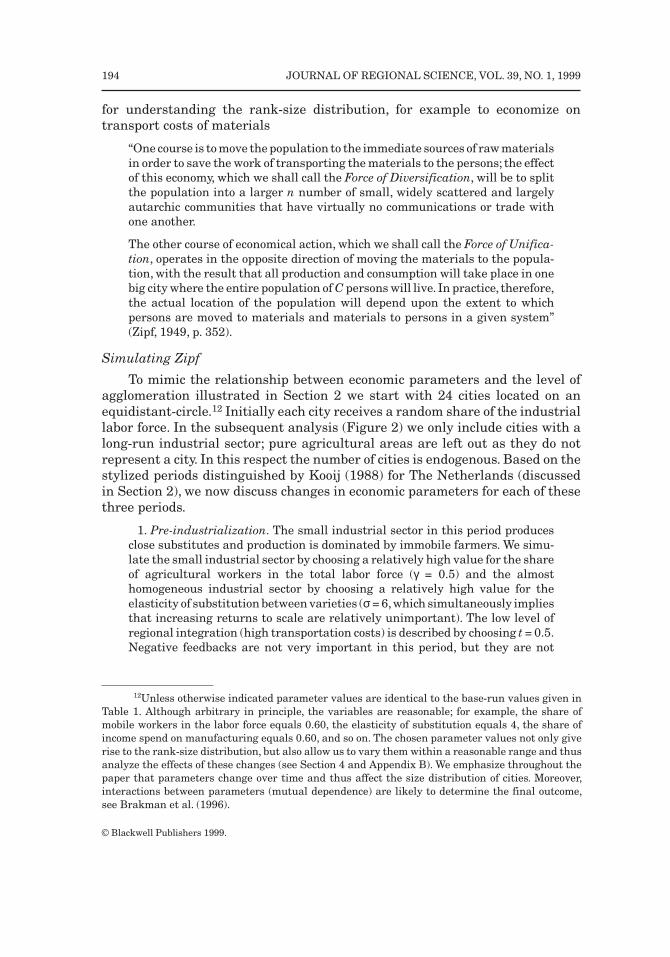
for understanding the rank-size distribution, for example to economize ontransport costs of materials

“One course is to move the population to the immediate sources of raw materialsin order to save the work of transporting the materials to the persons; the effectof this economy, which we shall call the Force of Diversification, will be to splitthe population into a larger n number of small, widely scattered and largelyautarchic communities that have virtually no communications or trade withone another.

The other course of economical action, which we shall call the Force of Unifica-tion, operates in the opposite direction of moving the materials to the popula-tion, with the result that all production and consumption will take place in onebig city where the entire population of C persons will live. In practice, therefore,the actual location of the population will depend upon the extent to whichpersons are moved to materials and materials to persons in a given system”(Zipf, 1949, p. 352).

Simulating Zipf

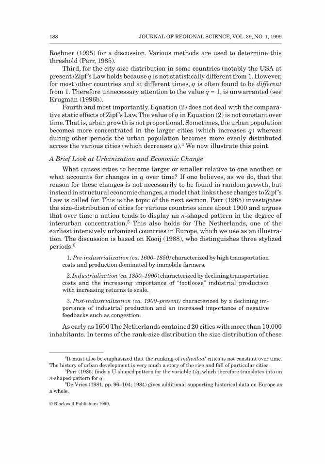
To mimic the relationship between economic parameters and the level ofagglomeration illustrated in Section 2 we start with 24 cities located on anequidistant-circle.12 Initially each city receives a random share of the industriallabor force. In the subsequent analysis (Figure 2) we only include cities with along-run industrial sector; pure agricultural areas are left out as they do notrepresent a city. In this respect the number of cities is endogenous. Based on thestylized periods distinguished by Kooij (1988) for The Netherlands (discussedin Section 2), we now discuss changes in economic parameters for each of thesethree periods.

1. Pre-industrialization. The small industrial sector in this period producesclose substitutes and production is dominated by immobile farmers. We simu-late the small industrial sector by choosing a relatively high value for the shareof agricultural workers in the total labor force (γ = 0.5) and the almosthomogeneous industrial sector by choosing a relatively high value for theelasticity of substitution between varieties (σ = 6,which simultaneously impliesthat increasing returns to scale are relatively unimportant). The low level ofregional integration (high transportation costs) is described by choosing t = 0.5.Negative feedbacks are not very important in this period, but they are not

12Unless otherwise indicated parameter values are identical to the base-run values given inTable 1. Although arbitrary in principle, the variables are reasonable; for example, the share ofmobile workers in the labor force equals 0.60, the elasticity of substitution equals 4, the share ofincome spend on manufacturing equals 0.60, and so on. The chosen parameter values not only giverise to the rank-size distribution, but also allow us to vary them within a reasonable range and thusanalyze the effects of these changes (see Section 4 and Appendix B). We emphasize throughout thepaper that parameters change over time and thus affect the size distribution of cities. Moreover,interactions between parameters (mutual dependence) are likely to determine the final outcome,see Brakman et al. (1996).



absent (think of the disease-ridden large cities in the Middle Ages) which issimulated by choosing a moderate value for τ , τ = 0.25.

2. Industrialization. The basic characteristic in this period is the spectaculardecrease in transportation costs and the increasing importance of footlooseindustrial production with increasing returns to scale. At the same timenegative feedbacks are not absent, but also not very important in the sense thatthey prevent large cities becoming even larger. In the model we simulate thesefactors by lowering transport costs to t = 0.8 (remember, a high value of t impliesa low level of transportation costs) and increasing the share of the industriallabor force in total employment, γ = 0.6. The increased importance of economiesof scale and differentiated industrial products are represented by choosingσ = 4. In this period the strong industrialization leads to the disappearance ofsmall cities.This corresponds with the idea that agglomerating forces dominateduring the era of big-city growth.

3. Post-industrialization. In this period transportation costs remain low andas before the industrial sector is characterized by differentiated products andincreasing returns to scale. The notable difference with earlier periods iscongestion, such as the growing traffic jams, air pollution, and rising land rentsin cities. Smaller cities are less troubled by such effects and therefore have atendency to grow faster. In the model we simulate this by increasing thecongestion parameter τ to 0.5.

Figure 2 presents some simulation results for the above three periods. Atleast 93 percent of the variance in city size is explained by the rank-sizedistribution. More importantly, these simulations suggest that the n-shapedpattern of q over time, identified by Parr (1985), depends on the economicparameter changes. Thus, in principle, we can reproduce rank-size distributionsby varying those parameters that have been identified in the literature to berelevant for understanding the changes in the size distribution of cities.

4. STRUCTURAL ANALYSIS

In Section 3 we demonstrate that it is possible to derive a size distributionof cities generating the rank-size distribution based on an explicit general-equi-librium location model. The question arises whether or not rank-size distribu-tions are a structural outcome of our model. First, we analyze the migrationdynamics inherent in the adjustment process of the model for a particularexample using the base-run parameter values and a random initial distributionof the mobile labor force. Second, we analyze whether the economic model isimportant in increasing the explanatory power of the rank-size distribution.Third, we investigate the impact of changes in economic parameters on q andthe power of agglomeration. Finally, the complex nature of the impact oftransportation costs on agglomeration induces us to analyze a somewhat moregeneral spatial structure.



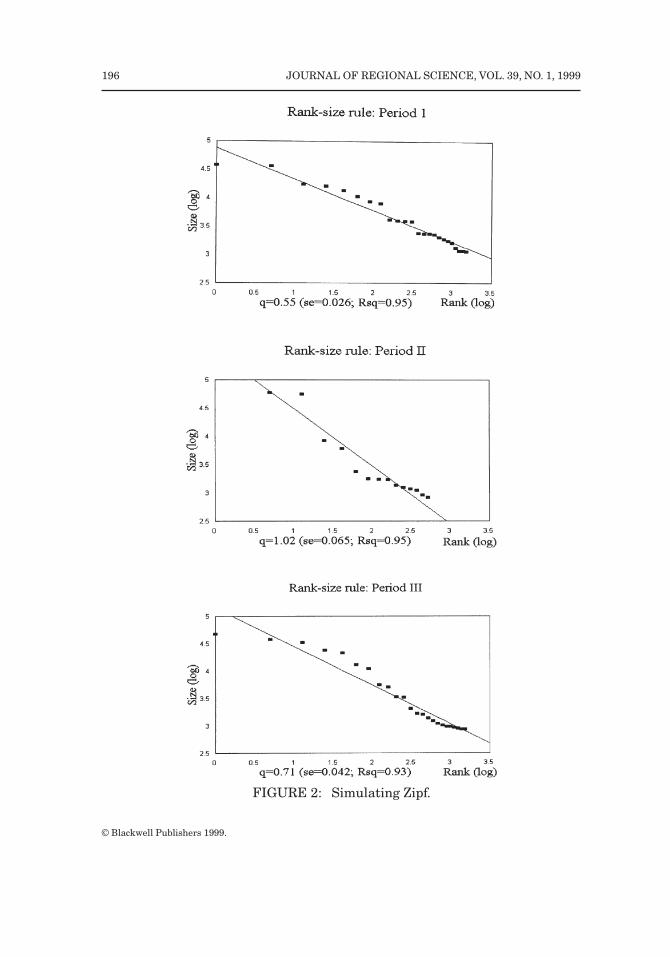
FIGURE 2: Simulating Zipf.



Adjustment

Analyzing more closely the adjustment over time of a typical simulationexample is the best way to get an intuitive feel for the adjustment process.13

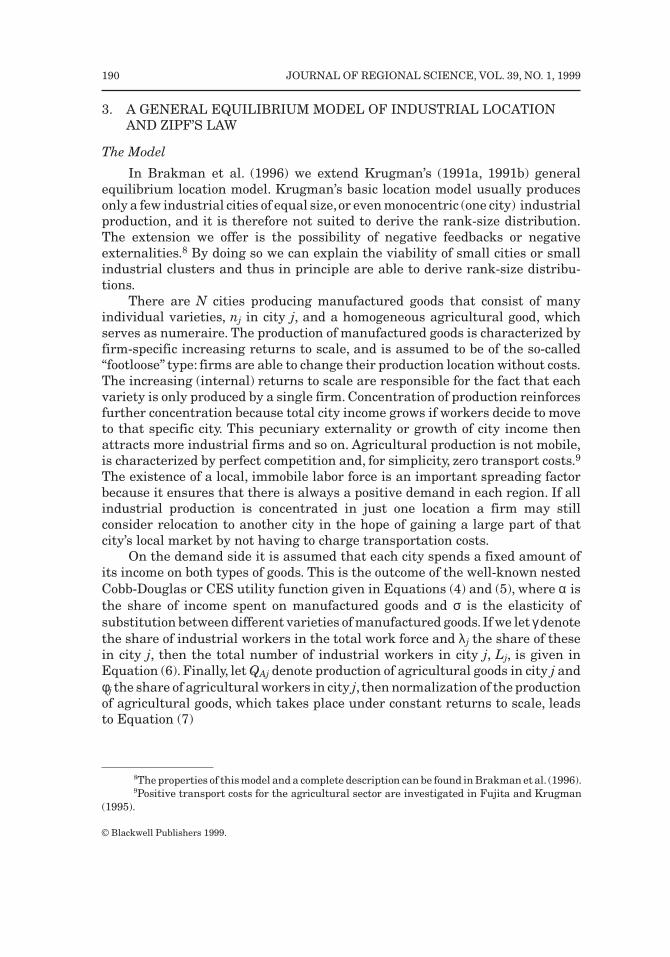
Figure 3a depicts a random initial distribution of city size over the 24 cities onthe equidistant circle.14 Given this initial distribution we solve for the short-runequilibrium. The real wages for industrial workers differ between the 24 citieswhich starts a migration process of workers from cities with low real wages tocities with high real wages according to Equation (23) in Appendix 1. Theredistribution of workers determines a new short-run equilibrium and starts asecond migration process because the real wages are still not equal for all cities.The process continues until the long-run equilibrium is reached, in this simula-tion example, after 16 migration process. Figure 3b depicts the final distributionof city size over the 24 cities at the long-run equilibrium. Ultimately there aretwo agglomeration centers of economic activity: one center around City 1 andone center around City 12.

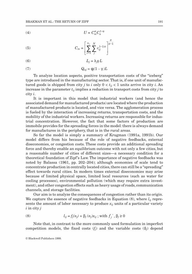
Inspecting both panels of Figure 3 shows that the two final centers ofeconomic agglomeration are close to the initial centers of high economic activity.At the same time, the two final centers are rather evenly spread over theequidistant circle, that is they are not too close to each other. This is also clearfrom Figure 4a, showing the evolution of size over time as a result of themigration process for Cities 1, 2, 11, and 12 (ultimately ranked number 1–3 and5 in size). After two migration processes, Cities 2 and 11 are the largest cities.However, as agglomeration centers these two cities are too close to each other;therefore City 2 ultimately becomes smaller than City 1 and City 12 becomessubstantially larger than City 11. As demonstrated by City 11, the adjustmentprocess is not monotone over time.15 The prosperity of individual cities does notdepend only on its own size,but also on that of its neighbors. City 14, for example,is initially the largest city. However, it is surrounded by smaller cities so itultimately drops in the rankings to number 7. Nonetheless, initial size doesmatter: eight out of the ten ultimately largest cities were in the initial top tenlist.

Finally, Figure 4b suggests that the model increases the predictive powerof the rank-size distribution: as the city size distribution is adjusting to thelong-run equilibrium the share of the variance explained by the rank-sizedistribution is increasing (until the level R2 = 0.95 is reached). Simultaneously,the level of agglomeration as measured by the q-value is increasing over time

13This approach was suggested to us by an anonymous referee. The parameter values we useare given in Table 1.

14The uniform random distribution is used to determine the industrial labor force for the 24cities.However,note that Figure 3 depicts total city size, that is the sum of industrial and agriculturalworkers.

15The size of Cities 1, 12, 13, and 24 is monotone increasing; of Cities 5, 6, 8, 14, 15, 18, 19, 20,21, and 23 is monotone decreasing; and of the remaining ten cities is first increasing and thendecreasing.



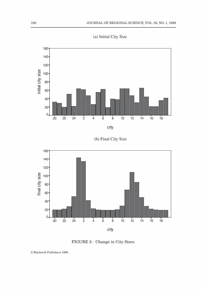
FIGURE 3: Change in City Sizes.



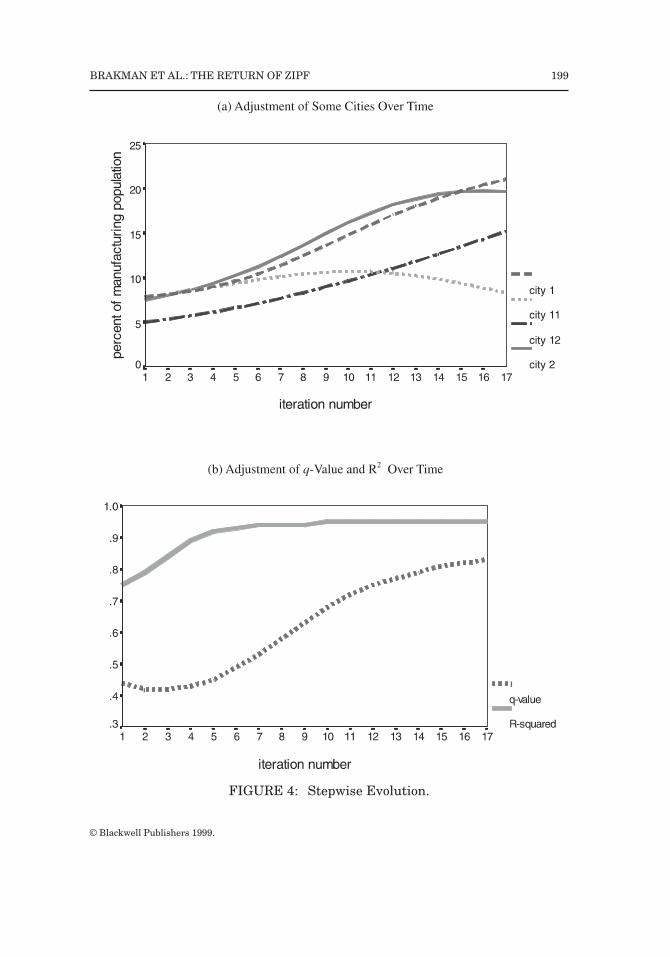
FIGURE 4: Stepwise Evolution.



after a small initial drop. However, this is only one example. We know that inthis type of nonlinear model initial conditions may be very important in deter-mining the final equilibrium. We now examine this in more detail.

Does the Model Matter?

We first test the rank-size distribution without using the model, that is bydrawing (10,000 times) a random distribution of the mobile labor force for eachof the 24 cities from the uniform distribution and calculating the q value for eachdraw.16 This experiment results in a single-peaked distribution of q values witha wide range (from 0.3 to 1.7), an average fit (R2) of only 0.54 and an averaget-value of 5.3, see Table 1. Second, we repeatedly draw (240 times for the basescenario) an initial random distribution of the mobile labor force (also using theuniform distribution) to derive the concomitant long-run equilibrium for eachdraw applying the model. This procedure allows us to estimate the rank-sizedistribution, that is, we derive 240 q’s. The resulting frequency distribution of qis depicted in Figure 5, which leads us to distinguish between two possible setsof spatial outcomes: agglomeration (q > 0.725) and spreading (q < 0.725). Seebelow for a discussion of this criterion. Remarkably, the economic model gener-ates the rank-size distribution fairly adequately both if agglomeration or spread-ing occurs, although the former slightly outperforms the latter. See Table 1 forthese results and the selected base-run values for the parameters. More specifi-cally, under agglomeration the average share of the explained variance in citysize (i.e., R2) equals 0.94 with an average t-value of 19.8, whereas if spreadingoccurs the explained variance in city size equals 0.88 with an average t-value of14.5. Thus, inclusion of the model considerably increases the explanatory powerof the rank-size distribution. As we observed in Figure 2, the model is able toexplain changes in q, which is not the case with the stochastic approach.

Figure 5 illustrates three main points regarding the sensitivity of therank-size distribution with respect to changes in initial conditions. First, a largerange of long-run equilibrium outcomes is possible (q ranges from 0.24 to 0.88).17

Second, the simulated density function is double-peaked. The lower peak at theleft for low values of q, and thus relatively equally-sized cities, arises if the initialdistribution of the mobile labor force is relatively even.18 The much higher peak

16Alternative initial random distributions, with the obvious exception of the Pareto distribu-tion (see Read, 1988), may also be used to investigate whether our model adds to the explanatorypower of the rank-size distribution. No alternative initial distribution, not even the Pareto distribu-tion, can be used for more fundamental questions, such as the changes in the distribution resultingfrom parameter changes.

17As noted in Appendix A, the range of long-run equilibrium outcomes is affected by thevariable ε in Table 1. In the simulations a long-run equilibrium is reached if the relative deviationof the real wage does not exceed the value ε for each city.

18The reader should keep in mind that an exactly even distribution of the mobile labor forceover the 24 cities of the equidistant-circle is a long-run equilibrium for all parameter settings in thesequel.



at the right arises if the initial distribution is more uneven, which triggers aprocess of agglomeration. Third, Figure 5 suggests there is a dominant under-lying value of q characteristic of the base-run parameter setting (approximatelyq = 0.87). These three features do not depend on the specific base-run parametervalues but also apply for other parameter values (see Appendix 2 for some of thecorresponding simulated density functions). The double-peak and narrow rangeof Figure 5 is a reflection of the underlying economic structure of our model anda reminder of the interaction between economic parameter values and path-dependency.

After inspection of the double-peaked density functions we decided tosubdivide all simulation experiments into two groups: agglomeration andspreading. Henceforth, agglomeration takes place if the predicted value of thelargest city is at least ten times as large as the smallest city. This, admittedlyarbitrary, rule translates into a value of q = 0.725 and is based on the bi-modalfeature of Figure 5. However, the value q = 0.725 is an intermediate value for qfound in empirical studies (Parr, 1985; De Vries, 1981). In short, if q exceeds0.725 we will say agglomeration takes place, otherwise spreading occurs. Forexample, the mean q-value for the agglomeration subgroup of the base scenario(q = 0.853, see Table 2) leads to an average predicted value of the largest cityequal to fifteen times the smallest city if agglomeration takes place. In contrast,the mean q-value for the spreading subgroup of the base scenario (q = 0.437, seeTable 3) leads to an average predicted value of the largest city equal to only fourtimes the smallest city if spreading occurs.

FIGURE 5: Histogram of Base-Run Scenario.



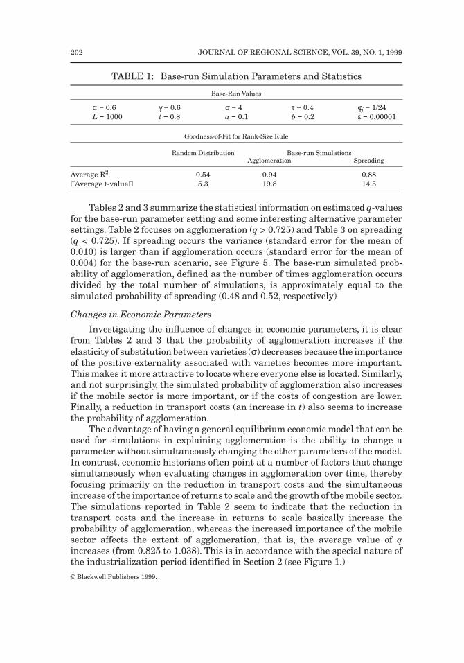
Tables 2 and 3 summarize the statistical information on estimated q-valuesfor the base-run parameter setting and some interesting alternative parametersettings. Table 2 focuses on agglomeration (q > 0.725) and Table 3 on spreading(q < 0.725). If spreading occurs the variance (standard error for the mean of0.010) is larger than if agglomeration occurs (standard error for the mean of0.004) for the base-run scenario, see Figure 5. The base-run simulated prob-ability of agglomeration, defined as the number of times agglomeration occursdivided by the total number of simulations, is approximately equal to thesimulated probability of spreading (0.48 and 0.52, respectively)

Changes in Economic Parameters

Investigating the influence of changes in economic parameters, it is clearfrom Tables 2 and 3 that the probability of agglomeration increases if theelasticity of substitution between varieties (σ) decreases because the importanceof the positive externality associated with varieties becomes more important.This makes it more attractive to locate where everyone else is located. Similarly,and not surprisingly, the simulated probability of agglomeration also increasesif the mobile sector is more important, or if the costs of congestion are lower.Finally, a reduction in transport costs (an increase in t) also seems to increasethe probability of agglomeration.

The advantage of having a general equilibrium economic model that can beused for simulations in explaining agglomeration is the ability to change aparameter without simultaneously changing the other parameters of the model.In contrast, economic historians often point at a number of factors that changesimultaneously when evaluating changes in agglomeration over time, therebyfocusing primarily on the reduction in transport costs and the simultaneousincrease of the importance of returns to scale and the growth of the mobile sector.The simulations reported in Table 2 seem to indicate that the reduction intransport costs and the increase in returns to scale basically increase theprobability of agglomeration, whereas the increased importance of the mobilesector affects the extent of agglomeration, that is, the average value of qincreases (from 0.825 to 1.038). This is in accordance with the special nature ofthe industrialization period identified in Section 2 (see Figure 1.)

TABLE 1: Base-run Simulation Parameters and Statistics

Base-Run Values

α = 0.6 γ = 0.6 σ = 4 τ = 0.4 φj = 1/24L = 1000 t = 0.8 a = 0.1 b = 0.2 ε = 0.00001

Goodness-of-Fit for Rank-Size Rule

Random Distribution Base-run SimulationsAgglomeration Spreading

Average R2 0.54 0.94 0.88Average t-value 5.3 19.8 14.5



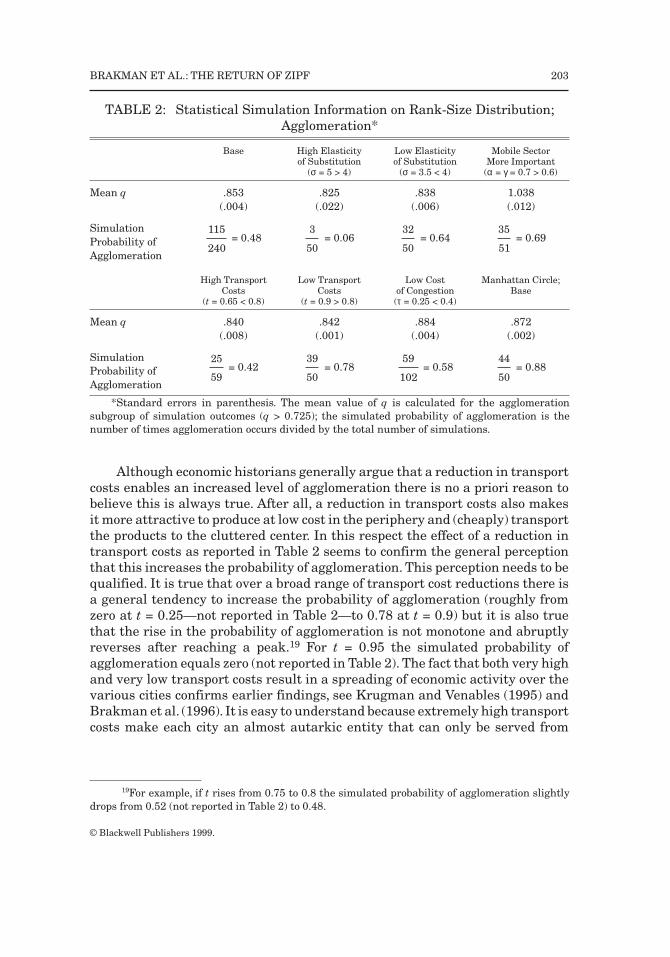
Although economic historians generally argue that a reduction in transportcosts enables an increased level of agglomeration there is no a priori reason tobelieve this is always true. After all, a reduction in transport costs also makesit more attractive to produce at low cost in the periphery and (cheaply) transportthe products to the cluttered center. In this respect the effect of a reduction intransport costs as reported in Table 2 seems to confirm the general perceptionthat this increases the probability of agglomeration. This perception needs to bequalified. It is true that over a broad range of transport cost reductions there isa general tendency to increase the probability of agglomeration (roughly fromzero at t = 0.25—not reported in Table 2—to 0.78 at t = 0.9) but it is also truethat the rise in the probability of agglomeration is not monotone and abruptlyreverses after reaching a peak.19 For t = 0.95 the simulated probability ofagglomeration equals zero (not reported in Table 2). The fact that both very highand very low transport costs result in a spreading of economic activity over thevarious cities confirms earlier findings, see Krugman and Venables (1995) andBrakman et al. (1996). It is easy to understand because extremely high transportcosts make each city an almost autarkic entity that can only be served from

TABLE 2: Statistical Simulation Information on Rank-Size Distribution;Agglomeration*

Base High Elasticity Low Elasticity Mobile Sectorof Substitution of Substitution More Important

(σ = 5 > 4) (σ = 3.5 < 4) (α = γ = 0.7 > 0.6)

Mean q .853 .825 .838 1.038(.004) (.022) (.006) (.012)

SimulationProbability ofAgglomeration

= 0.48 = 0.06 = 0.64 = 0.69

High Transport Low Transport Low Cost Manhattan Circle;Costs Costs of Congestion Base

(t = 0.65 < 0.8) (t = 0.9 > 0.8) (τ = 0.25 < 0.4)

Mean q .840 .842 .884 .872(.008) (.001) (.004) (.002)

SimulationProbability ofAgglomeration

= 0.42 = 0.78 = 0.58 = 0.88

*Standard errors in parenthesis. The mean value of q is calculated for the agglomerationsubgroup of simulation outcomes (q > 0.725); the simulated probability of agglomeration is thenumber of times agglomeration occurs divided by the total number of simulations.

115

240

3

50

32

50

35

51

25

59

39

50

59

102

44

50

19For example, if t rises from 0.75 to 0.8 the simulated probability of agglomeration slightlydrops from 0.52 (not reported in Table 2) to 0.48.



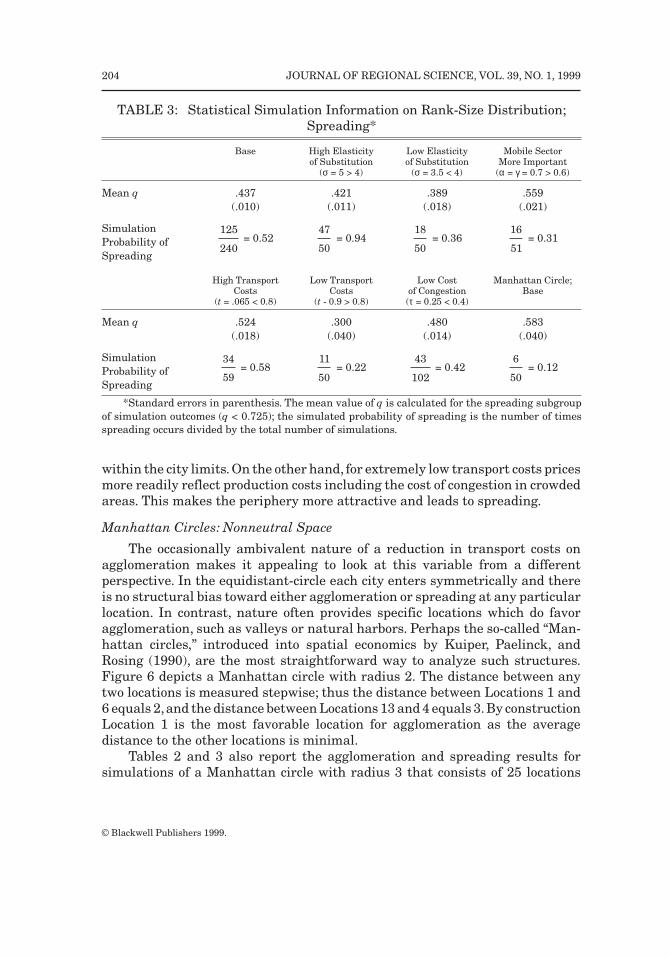
within the city limits. On the other hand, for extremely low transport costs pricesmore readily reflect production costs including the cost of congestion in crowdedareas. This makes the periphery more attractive and leads to spreading.

Manhattan Circles: Nonneutral Space

The occasionally ambivalent nature of a reduction in transport costs onagglomeration makes it appealing to look at this variable from a differentperspective. In the equidistant-circle each city enters symmetrically and thereis no structural bias toward either agglomeration or spreading at any particularlocation. In contrast, nature often provides specific locations which do favoragglomeration, such as valleys or natural harbors. Perhaps the so-called “Man-hattan circles,” introduced into spatial economics by Kuiper, Paelinck, andRosing (1990), are the most straightforward way to analyze such structures.Figure 6 depicts a Manhattan circle with radius 2. The distance between anytwo locations is measured stepwise; thus the distance between Locations 1 and6 equals 2,and the distance between Locations 13 and 4 equals 3.By constructionLocation 1 is the most favorable location for agglomeration as the averagedistance to the other locations is minimal.

Tables 2 and 3 also report the agglomeration and spreading results forsimulations of a Manhattan circle with radius 3 that consists of 25 locations

TABLE 3: Statistical Simulation Information on Rank-Size Distribution;Spreading*

Base High Elasticity Low Elasticity Mobile Sectorof Substitution of Substitution More Important

(σ = 5 > 4) (σ = 3.5 < 4) (α = γ = 0.7 > 0.6)

Mean q .437 .421 .389 .559(.010) (.011) (.018) (.021)

SimulationProbability ofSpreading

= 0.52 = 0.94 = 0.36 = 0.31

High Transport Low Transport Low Cost Manhattan Circle;Costs Costs of Congestion Base

(t = .065 < 0.8) (t - 0.9 > 0.8) (τ = 0.25 < 0.4)

Mean q .524 .300 .480 .583(.018) (.040) (.014) (.040)

SimulationProbability ofSpreading

= 0.58 = 0.22 = 0.42 = 0.12

*Standard errors in parenthesis. The mean value of q is calculated for the spreading subgroupof simulation outcomes (q < 0.725); the simulated probability of spreading is the number of timesspreading occurs divided by the total number of simulations.

125

240

47

50

18

50

16

51

34

59

11

50

43

102

6

50



using the base-run parameter setting.20 As expected, the structural bias towardagglomeration considerably increases the simulated probability of agglomera-tion (from 0.48 to 0.88, see Table 2). However, two aspects are more surprising.First, agglomeration is not automatic because occasionally spreading occurs.Second, despite its structural advantage in the center of the Manhattan circleLocation 1 is not always the largest location in the long-run equilibrium. Thisis illustrated in Figure 7 where panel a depicts a typical outcome in whichLocation 1 is the largest and panel b depicts a more exceptional outcome in whichan off-center location is the largest.21 It is a reminder of the fact that thestructural advantage of Location 1 is not always decisive in making it the largestlocation; sometimes path-dependency may be more important. None of thesimulations with the Manhattan circle achieve the circular-like, transport-cost–minimizing agglomeration results in which Location 1 is smaller thanequal-sized Locations 2, 3, 4, and 5 as reported in Kuiper, Kuiper, and Paelinck(1993), not even if we start with an even distribution of the mobile labor force.

5. CONCLUSIONS

One rarely finds empirical relationships in economics which deserve to becalled “laws.” Zipf ’s Law is a noteworthy exception. Despite impressive progressin the theory of city formation and city systems in recent decades, the theoreticeconomic foundation is still poorly understood. In this paper we provide somefurther understanding of Zipf ’s Law by incorporating congestion in an economiclocation model. In our analysis economic parameters play an explicit role indetermining the rank-size distribution and describing its evolution over time.The model is able to derive the rank-size distribution because the equality of

6

13 2 7

12 5 1 3 8

11 4 9

10

FIGURE 6: Manhattan Circle with Radius 2.

20The number of locations of a Manhattan circle with radius R equals 2 R(R + 1) + 1.21Location 1 was the largest location in the long-run equilibrium in 42 of the 50 simulations.



(a) Center Location is Largest

(b) Center Location is Not Largest

FIGURE 7: Simulations with Manhattan Circles.



agglomerating and spreading forces allows for the simultaneous existence oflarge and small cities.

Using historical data for The Netherlands as an illustration, we are roughlyable to reconstruct historical trends with respect to the rank-size distributionby varying parameters that represent specific economic factors (such as theshare of the industrial labor force in total employment, the level of integrationbetween cities, congestion, and the type of goods). The parameters we use in oursimulations are found to be important by economic historians for describing(changes in) the size distributions of cities. Simulations show that these parame-ters have the expected effects.

Furthermore, we show that the rank-size distribution is a structural out-come of our model. By repeatedly drawing an initial distribution of the mobilelabor force from a uniform distribution we determine simulated long-run equi-librium density functions for q. This results in a double-peaked density function;a lower peak if the initial distribution of the mobile labor force is relatively evenand a higher peak if the initial distribution is more uneven. It is demonstratedthat our model considerably increases the explanatory power of the rank-sizedistribution. All in all, it seems possible to derive Zipf ’s Law from a general-equilibrium location model.

REFERENCESAbdel-Rahman, Hesham M. 1994. “Economies of Scope in Intermediate Goods and a System of

Cities,” Regional Science and Urban Economics, 24, 497–524.Abdel-Rahman, Hesham M. and Masahisa Fujita. 1993. “Specialization and Diversification in a

System of Cities,” Journal of Urban Economics, 33, 189–222.Ades, Alberto and Edward Glaeser. 1997. “Trade and Circuses, Explaining Urban Giants,” Quarterly

Journal of Economics, 110, 195–227.Arnott, Richard and Kenneth Small. 1994. “The Economics of Traffic Congestion,” American

Scientist, 446–455.Auerback, Felix, 1913. “Das Gesetz der Bevoelkerungskoncentration,” Petermanns Geographische

Mitteilungen, 59, 74–76.Balassa, Bela. 1961. The Theory of Economic Integration. New York: Allen and Unwin.Brakman, Steven and Harry Garretsen. 1993. “The Relevance of Initial Conditions for the German

Unification,” Kyklos, 46, 163–181.Brakman, Steven, Harry Garretsen, Richard Gigengack, Charles van Marrewijk, and Rien Wagen-

voort. 1996. “Negative Feedbacks in the Economy and Industrial Location,” Journal of RegionalScience, 36, 631–652.

Bura, Stéphane, France Guérin-Pace, Hélène Mathian, Denise Pumian, and Lena Sanders. 1996.“Multiagent Systems and the Dynamics of a Settlement System,” Geographical Analysis, 28,161–178.

Christaller, Walter. 1933. Central Places in Southern Germany (Fischer, transl.). London: PrenticeHall.

de Vries, Jan. 1981. “Patterns of Urbanization in Pre-Industrial Europe, 1500–1800,” in H. Schmal(ed.), Patterns of European Urbanization since 1500, London: Croom Helm, pp. 79–109.

———. 1984. European Urbanization 1500–1800, London: Methuen.Eaton, Curtis B. and Richard G. Lipsey. 1982. “An Economic Theory of Central Places,” The Economic

Journal, 92, 56–72.Eaton, Jonathan and Zvi Eckstein. 1997. “Cities and Growth: Theory and Evidence from France and

Japan,” Regional Science and Urban Economics, 27, 443–474.



Fujita, Masahisa. 1989. Urban Economic Theory; Land Use and City Size. Cambridge: CambridgeUniversity Press.

Fujita, Masahisa, Hideaki Ogawa, and Jacques-François Thisse. 1988. “A Spatial CompetitionApproach to Central Place Theory: Some Basic Principles,” Journal of Regional Science, 28,477–494.

Fujita, Masahisa and Paul R. Krugman. 1995. “When Is the Economy Monocentric?: von Thünenand Chamberlin Unified,” Regional Science and Urban Economics, 25, 505–528.

Fujita, Masahisa and Jacques-François Thisse. 1996. “Economics of Agglomeration,” Journal of theJapanese and International Economies, 10, 339–378.

Glaeser, Edward L., Hedi D. Kallal, José Scheinkman, and Andrei Schleifer. 1992. “Growth in Cities,”Journal of Political Economy, 100, 1126–1152.

Goodrich, Ernest. 1925. “The Statistical Relationship between Population and the City Plan.” in E.R. Burgess (ed.), The Urban Community. Chicago: The University of Chicago Press, pp. 144–150.

Haag, Günther and Horst Max. 1995. “Rank-Size Distribution of Settlement Systems,” Papers inRegional Science, 74, 243–258.

Henderson,Vernon J.1974. “The Sizes and Types of Cities,”American Economic Review,64,640–656.———. 1977. Economic Theory and the Cities. New York: Academic Press.Kooij, Pim. 1988. “Peripheral Cities and Their Regions in the Dutch Urban System until 1900,”

Journal of Economic History, 48, 357–371.Krugman, Paul R. 1991. Geography and Trade, Cambridge, MA: Massacusetts Institute of Technol-

ogy.———. 1991b. “Increasing Returns and Economic Geography,” Journal of Political Economy, 99,

483–499.———. 1996a. The Self-Organizing Economy. Cambridge: Blackwell.———. 1996b. “Confronting the Mystery of Urban Hierarchy,” Journal of the Japanese and Interna-

tional Economies, 10, 399–418.Krugman, Paul R. and Anthony Venables. 1995. “Globalization and the Inequality of Nations,”

Quarterly Journal of Economics, 110, 857–880.Kuiper, Friso J., J. Hans Kuiper, and Jean H. P. Paelinck. 1993. “Tinbergen-Bos Metricised Systems:

Some Further Results,” Urban Studies, 30, 1745–1761.Kuiper, J. Hans, Jean H. P. Paelinck, and Ken E. Rosing. 1990. “Transport Flows in Tinbergen-Bos

Systems,” in K. Peschel (ed.), Infrastructure and the Space Economy, Heidelberg: Springer Verlag,pp. 29–52.

Lösch,August.1940.The Economics of Location (Fischer, transl.). New Haven:Yale University Press.Lotka, Alfred J. 1925. The Elements of Physical Biology. Baltimore: Williams and Wilkins.Mulligan, Gordon F. 1984. “Agglomeration and Central Place Theory: A Review of the Literature,”

International Regional Science Review, 9, 1–42.Parr,John B.1985. “A Note on the Size Distribution of Cities over Time,”Journal of Urban Economics,

18, 199–212.Quinzii, Martine and Jacques-François Thisse. 1990. “On the Optimality of Central Places,”

Econometrica, 58, 1101–1119.Read, Cambell B. 1988. “Zipf ’s Law,” in S. Kotz, N.L. Johnson, C.B. Read (eds.), Encyclopedia of

Statistical Sciences, New York: Wiley.Roehner, Bertrand Marie. 1995. “Evolution of Urban Systems in the Pareto Plane,” Journal of

Regional Science, 35, 277–300.Simon, Herbert. 1955. “On a Class of Skew Distribution Functions”, Biometrika, 425–440.Stewart, John Q. 1948. “Demographic Gravitation: Evidence and Applications,” Sociometry, 11,

31–58.Suh, Seoung H. 1991. “The Optimal Size Distribution of Cities,” Journal of Urban Economics, 30,

182–191.Zipf, George K. 1949. Human Behavior and the Principle of Least Effort, New York: Addison Wesley.



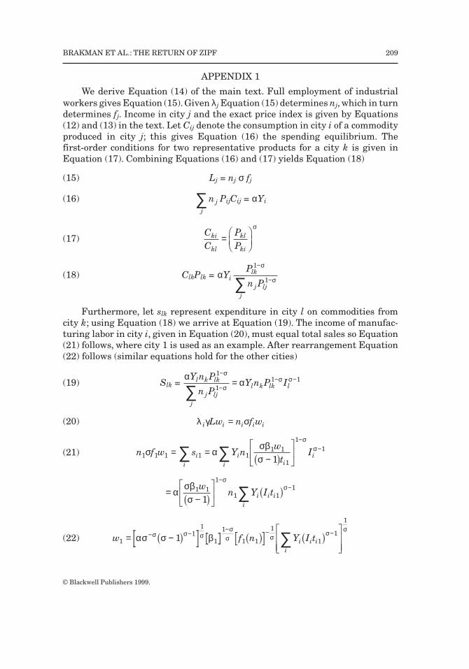
APPENDIX 1

We derive Equation (14) of the main text. Full employment of industrialworkers gives Equation (15). Given λj Equation (15) determines nj, which in turndetermines fj. Income in city j and the exact price index is given by Equations(12) and (13) in the text. Let Cij denote the consumption in city i of a commodityproduced in city j; this gives Equation (16) the spending equilibrium. Thefirst-order conditions for two representative products for a city k is given inEquation (17). Combining Equations (16) and (17) yields Equation (18)

(15) Lj = nj σ fj

(16) PijCij = αYi

(17)

(18) ClkPlk =

Furthermore, let slk represent expenditure in city l on commodities fromcity k; using Equation (18) we arrive at Equation (19). The income of manufac-turing labor in city i, given in Equation (20), must equal total sales so Equation(21) follows, where city 1 is used as an example. After rearrangement Equation(22) follows (similar equations hold for the other cities)

(19) Slk =

(20)

(21)

(22)

njj

∑

CC

PP

ki

kl

kl

ki=FHG

IKJ

σ

ασ

σY

P

n Pi

lk

j ljj

1

1

−

−∑

αα

σ

σσ σY n P

n PY n P Il k lk

j ljj

l k lk l

1

11 1

−

−− −

∑=

λ γ σi i i i iLw n f w=

n f w s Y nw

tIi

ii

i ii1 1 1 1 1

1 1

1

11

1σ α

σβσ

σσ= =

−LNM

OQP∑ ∑

−−

b g

=−

LNM

OQP

−−∑α

σβσ

σσ1 1

1

1 11

1w

n Y I tii

i ib g b g

w f n Y I tii

i i11

1

1

1

1 1

1

11

1

1= −LNMM

OQPP

− −− − −∑ασ σ βσ σ σ

σσ σ σ σ

b g b g b g



Finally, we note that , where ωj is the real wage in location j. Thechange in city j’s share of mobile labor is given in Equation (23) and driven bythe extent to which its wage deviates from the overall average . In

the simulations a long-run equilibrium is reached if the relative deviation of thereal wage does not exceed the value ε for each city.

(23) λj(s + 1) = λj(s) + ρλj(s)

APPENDIX 2. SIMULATED HISTOGRAMS

This appendix displays the simulated histograms of estimated q coefficientsfor low costs of congestion, low transport costs, low elasticity of substitution, highmobility, high elasticity of substitution, and high transport costs, respectively.

ω αj j jw I= −

ω λ ω= ∑ j jj

ω ωj s s+ −1b g b g



low cost of congestion

1,050,950

,850,750

,650,550

,450,350

,250,150

60

50

40

30

20

10

0

Std. Dev = ,21 Mean = ,714N = 102,00

low transport cost

1,101,05

1,00,95

,90,85

,80,75

,70,65

,60,55

,50,45

,40,35

,30,25

,20,15

40

30

20

10

0

Std. Dev = ,23 Mean = ,72N = 50,00

low elasticity of subs titution

1,101,05

1,00,95

,90,85

,80,75

,70,65

,60,55

,50,45

,40,35

,30,25

,20,15

30

20

10

0

Std. Dev = ,22Mean = ,68N = 50,00

FIGURE 8: Histograms for Other Parameters.



high mobility

1,101,05

1,00,95

,90,85

,80,75

,70,65

,60,55

,50,45

,40,35

,30,25

,20,15

16

14

12

10

8

6

4

2

0

Std. Dev = ,24 Mean = ,89N = 51,00

high elasticity of substitution

1,101,05

1,00,95

,90,85

,80,75

,70,65

,60,55

,50,45

,40,35

,30,25

,20,15

14

12

10

8

6

4

2

0

Std. Dev = ,12 Mean = ,45N = 50,00

high transport costs

1,101,05

1,00,95

,90,85

,80,75

,70,65

,60,55

,50,45

,40,35

,30,25

,20,15

16

14

12

10

8

6

4

2

0

Std. Dev = ,18 Mean = ,66N = 59,00



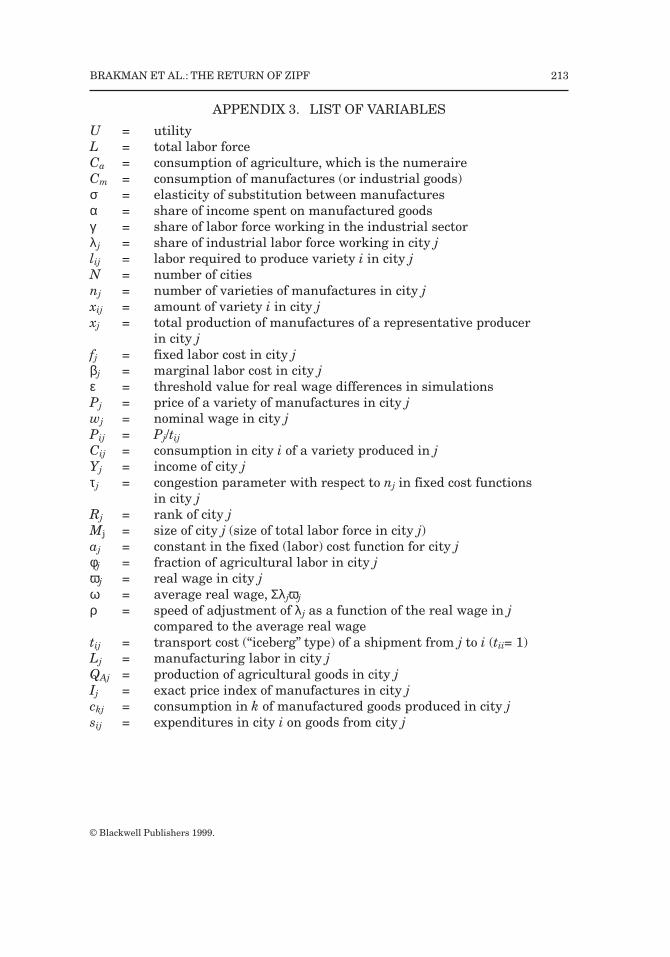
APPENDIX 3. LIST OF VARIABLES

U = utilityL = total labor forceCa = consumption of agriculture, which is the numeraireCm = consumption of manufactures (or industrial goods)σ = elasticity of substitution between manufacturesα = share of income spent on manufactured goodsγ = share of labor force working in the industrial sectorλj = share of industrial labor force working in city jlij = labor required to produce variety i in city jN = number of citiesnj = number of varieties of manufactures in city jxij = amount of variety i in city jxj = total production of manufactures of a representative producer

in city jfj = fixed labor cost in city jβj = marginal labor cost in city jε = threshold value for real wage differences in simulationsPj = price of a variety of manufactures in city jwj = nominal wage in city jPij = Pj/tijCij = consumption in city i of a variety produced in jYj = income of city jτj = congestion parameter with respect to nj in fixed cost functions

in city jRj = rank of city jMj = size of city j (size of total labor force in city j)aj = constant in the fixed (labor) cost function for city jφj = fraction of agricultural labor in city jωj = real wage in city jϖ = average real wage, Σλjωj

ρ = speed of adjustment of λj as a function of the real wage in jcompared to the average real wage

tij = transport cost (“iceberg” type) of a shipment from j to i (tii= 1)Lj = manufacturing labor in city jQAj = production of agricultural goods in city jIj = exact price index of manufactures in city jckj = consumption in k of manufactured goods produced in city jsij = expenditures in city i on goods from city j



the return of zipf: towards a further understanding … jrs 1999.p… · why do cities exist, and...

Documents