Graduate Theses, Dissertations, and Problem Reports

2019

Conceptual Design of MALE UAVs Conceptual Design of MALE UAVs

Vincent Spada Vincent Spada, vspada@mix.wvu.edu

Follow this and additional works at: https://researchrepository.wvu.edu/etd

Part of the Other Aerospace Engineering Commons

Recommended Citation Recommended Citation Spada, Vincent, "Conceptual Design of MALE UAVs" (2019). Graduate Theses, Dissertations, and Problem Reports. 7374. https://researchrepository.wvu.edu/etd/7374

This Problem/Project Report is protected by copyright and/or related rights. It has been brought to you by the The Research Repository @ WVU with permission from the rights-holder(s). You are free to use this Problem/Project Report in any way that is permitted by the copyright and related rights legislation that applies to your use. For other uses you must obtain permission from the rights-holder(s) directly, unless additional rights are indicated by a Creative Commons license in the record and/ or on the work itself. This Problem/Project Report has been accepted for inclusion in WVU Graduate Theses, Dissertations, and Problem Reports collection by an authorized administrator of The Research Repository @ WVU. For more information, please contact researchrepository@mail.wvu.edu.

Conceptual Design of MALE UAVs

Vincent P. Spada Jr.

Problem Report submitted

to The Statler College of Engineering and Mineral Resources

at West Virginia University

in partial fulfillment of the requirements for the degree of

Master of Science in

Aerospace Engineering

Peter D. Gall, Ph.D., Chair

Patrick Browning, Ph.D.

Wade W. Huebsch, Ph.D.

Department of Mechanical and Aerospace Engineering

Morgantown, West Virginia

2019

Keywords: Conceptual Design, Unmanned Aerial Vehicles, Supercomputer

Copyright 2019 Vincent Spada

ABSTRACT

Conceptual Design of MALE UAVs

Vincent P. Spada Jr.

The conceptual design process of aircraft involves the creation of a product, in this case

UAVS (unmanned aerial vehicles), using the most effective means possible across multiple sub-

disciplines of Aerospace Engineering. This paper will outline a unique methodology that involves

calculating certain design variables such as wing loading, power loading, aspect ratio and cruise

altitude in the conceptual design phase for MALE (medium altitude long endurance) UAVs.

Aircraft characteristics from MALE UAVs such as the MQ-9 predator and MQ-1 reaper will used

for a comparative aircraft study as “jumping off” points in order to carry out the initial calculations.

An intensive computational computer program was created to perform the appropriate

calculations in an iterative process. These calculations, details outlined in this paper, involved the

usage of both empirical and analytical weight equations, to calculate the s (structural factor), and

series of aerodynamic equations, to calculate the L/Dcrs (Lift over Drag at cruise) which are both

the termination criteria. The iterative process mainly involves cycling through numerous aspect

ratios, wing loadings and cruise altitudes to generate a family of aircraft that can be plotted against

lines of constant TOGW (take-off gross weight) and design constraint such as Landing and Takeoff

distances. The most efficient design can then be derived within the bounds of the design constraints

at the lowest TOGW.

Due to the intensive computational nature of the analytical method for calculating the

weight of the wing, a cluster computer made up of a series of Raspberry PIs was developed to ease

the computational time.

This unique design process was able to successfully allow the user to generate a MALE

UAV within certain design constraints per user request.

iii

Acknowledgments

I would like to first acknowledge my advisor and mentor Dr. Peter Gall. Dr. Gall has guided

me throughout both my undergraduate and graduate studies at WVU. I contribute my current status

as an Aerospace Engineer to his unconditional support. I would also like to thank my family for

all their love and support.

iv

Table of Contents

List of Tables ................................................................................................................................. v

List of Figures ............................................................................................................................... vi

List of Symbols ............................................................................................................................ vii

1. Introduction .............................................................................................................................. 1

2. Problem Statement.................................................................................................................... 1

3. Background Research ............................................................................................................... 1

3.1 Brief History of the UAV ..................................................................................................... 1

3.2 Conventional Design Approach ............................................................................................ 2

3.2 Cluster Computing ................................................................................................................ 3

3.2.1 Moore’s Law .................................................................................................................. 3

3.2.2 Aircraft Design and Supercomputers ............................................................................. 4

4. Methodology .............................................................................................................................. 5

4.1 Process of Conceptual Design .............................................................................................. 5

4.2 Preliminary Calculations of Parameters ................................................................................ 7

4.2.1 Comparative Aircraft Study ........................................................................................... 7

4.2.2 Engine Study .................................................................................................................. 8

4.2.3 Initialization of Takeoff Gross Weight .......................................................................... 9

4.2.4 Calculation of Aerodynamics ...................................................................................... 12

4.2.5 Calculation of Weights ................................................................................................ 14

4.2.6 TOGW Analysis........................................................................................................... 15

4.2.7 Design Constraint Analysis.......................................................................................... 16

4.2.7.1 Takeoff Distance ................................................................................................... 16

4.2.7.2 Landing Distance .................................................................................................. 20

4.3 Cluster Computer ................................................................................................................ 21

4.4 Verification and Validation................................................................................................. 23

5. Results and Discussion ............................................................................................................ 25

6. Conclusion ............................................................................................................................... 29

7. Future Work ............................................................................................................................ 30

References .................................................................................................................................... 32

Appenidx A .................................................................................................................................. 34

Appenidx B .................................................................................................................................. 36

Appenidx C .................................................................................................................................. 38

v

List of Tables

Table 1: User defined design constraint………………………………………………………...5

Table 2: Specifications from Comparative Aircraft Study……………………………………7

Table 3: Additional Specifications from Comparative Aircraft Study……………………….7

Table 4: Aerodynamic Parameters…………………………………………………………….17

vi

List of Figures

Figure 1: Traditional design process of aircraft defined by Corke. Blue represents the

design phases this report will focus on………………………………………………………….2

Figure 2: Advancement of the computer through time as it relates to transistor……………4

Figure 3: Methodology of the conceptual design process……………..……………………….6

Figure 4: General Atomics’ MQ-1 Predator…………………………………………….…….8

Figure 5: General Atomics’ MQ-9 Reaper…………………………………………………….8

Figure 6: Weight as a function of power for turbocharge engines……………………………9

Figure 7: Mission outline used for the fuel fraction in the computer program…………….10

Figure 8: Constant TOGW lines at an altitude of 20,000ft…………………………………..15

Figure 9: Constant TOGW lines at an altitude of 25,000ft…………………………………..16

Figure 10: CAD model of the cluster computer………………………………………………22

Figure 11: Flowchart representing the workflow through the cluster computer…………..23

Figure 12: Four levels of software testing……………………………………………………..23

Figure 13: Limits of the design constraints from regression testing………………………...24

Figure 14: Boundary testing results of the user defined design constraints……………...…25

Figure 15: Variant results with design constraints of R = 650nmi, E = 10hrs, Vcrs = 200kts,

Wpay = 2000lbs…………………………………………………………………………………. 25

Figure 16: TOGW constants for R = 650nmi, E = 10hrs, Vcrs = 200kts, Wpay = 2000 lbs….26

Figure 17: Variant results with design constraints of R = 250nmi, E = 15hrs, Vcrs = 150kts,

Wpay = 3000 lbs………………………………………………………………………………….27

Figure 18: TOGW constants for R = 250 nmi, E = 15 hrs, Vcrs = 150 kts, Wpay = 3000 lbs..28

Figure 19: MQ-9 developed in CAD…………………………………………………………...35

Figure 20: MQ-1 developed in CAD…………………………………………………………...35

Figure 21: Convergence Data GUI…………………………………………………………….37

Figure 22: Resource Center GUI………………………………………………………………37

vii

List of Symbols

Symbol Definition Units

ax x component of acceleration ft2/sec

Ap area of the propeller disk ft

AR aspect ratio ---

AReff effective aspect ratio ---

B wing span ft

Cd0 zero lift drag coefficient ---

CD0fus zero lift drag coefficient of fuselage ---

CD0HT zero lift drag coefficient of horizontal tail ---

CD0VT zero lift drag coefficient of vertical tail ---

CD0wing zero lift drag coefficient of wing ---

CF coefficient of friction ---

cf chord of flap ft

CL coefficient of lift ---

𝐶�̅� ratio of CLcr over CLL/Dmax ---

CLα wing angle of attack lift coefficient ---

CLcr coefficient of lift at cruise ---

CLL/Dmax coefficient of lift at L/Dmax ---

Clmax maximum lift coefficient ---

cr chord at wing root ft

ct chord at wing tip ft

CHT horizontal tail coefficient ---

CVT vertical tail coefficient ---

D drag lbs

Dx x component of drag lbs

e Oswald Efficiency Factor ---

Ff friction force lbs

h height of wing above ground ft

hTR transition height ft

iw incidence of the wing deg

L/Dcrs lift over drag at cruise ---

L/Dmax max. lift over drag ratio ---

lHT length from wing ¼ m.a.c to h. tail ¼ m.a.c ft

Lt length from wing ¼ m.a.c to tail ¼ m.a.c ft

lVT length from wing ¼ m.a.c to v. tail ¼ m.a.c ft

Lx x component of lift lbs

m.a.c. mean aerodynamic chord ft

Nz ultimate load factor ---

Preqd required shaft horsepower HP

PSHP shaft horsepower HP

viii

q dynamic pressure psf

R range n.m.

Re Reynolds Number ---

RTR transition phase arc length ft

SA approach distance ft

Sf fuselage wetted area ft2

SFR free roll distance ft

SHT horizontal tail area ft2

Sref wing reference area ft2

STR transition distance ft

SVT vertical tail reference area ft2

Sw trapezoidal area ft2

Swet wetted area ft2

Sw fus wetted area of the fuselage ft2

Sw HT wetted area of the horizontal tail ft2

Sw VT wetted area of the vertical tail ft2

Sw wing wetted area of the wing ft2

Tstatic static thrust lbs

Tx x component of thrust lbs

Vcr cruising velocity knots

Vhold/reserve holding and reserve velocity knots

VS0 stall velocity ft/sec

W weight lbs

Wdg design gross weight lbs

Wfw weight of fuel in wing lbs

Wfw weight of fuel in wing lbs

W/Sw wing loading lbs/ft2

Wstr structural weight lbs

WT0 take-off weight lbs

ηp propeller efficiency ---

αeff effective angle of attack deg

α0L zero lift angle of attack deg

Δαf change in angle of flaps deg

ΔCD change in drag coefficient ---

Δt change in time sec

Λ wing sweep deg

λ taper ratio ---

θ pitch angle deg

ϒ climb angle deg

μ friction coefficient

ρ density sl/ft3

1

1. Introduction

The conceptual design of an aircraft is a very extensive and sensitive process. The aviation

industry constantly attempts to improve previous designs and produce more efficient aircraft to

maximize output, minimize costs, and improve overall performance. The goal of this design effort

is to formulate a method to maximize efficiency in the creation of an UAV. This design method

will allow parameters such as takeoff gross weight and takeoff or landing distance to be minimized

while maximizing the efficiency of the aircraft for a set of desired performance characteristics.

Other more basic design methods may yield an inefficient aircraft which is overpowered,

excessively heavy, or includes unnecessary design measures due to the design being constrained

to one parameter.

2. Problem Statement

A computer algorithm is developed to apply a unique iterative methodology for the design

of MALE, cruising altitude < 35,000ft, UAVs with the assistance of inexpensive cluster

computing. This methodology will produce a family of aircraft that will calculate a specific set of

design variables such as W/S wing loading, W/P (power loading), AR (aspect ratio) and cruise

altitude to determine the aircraft with the lowest TOGW that meet design constraints set by the

user such as endurance, range as well as others. A cluster computer, developed from a series of

Raspberry PIs, was designed to ease this computational process.

3. Background Research

3.1. Brief History of the UAV

The development of the UAV can be traced back to the American Civil War when an

inventor loaded a hot air balloon with explosives that was set to drop on enemy forces when a

timed mechanism destroyed the balloon. One of the first aerial reconnaissance photos can be

credited to the American military during the Spanish-American war when an engineer tied a

camera to a kite that flew over enemy fortifications.

One of the biggest leaps in UAV design came during the end of WW2 when the NAZIS

deployed the Vengeance Weapon 1, also known as the V1. This weapon was designed to fly

2

explosives across the channel and crash into British cities. The effectiveness of this missile during

that war is debatable, however, its development throughout the 20th century has completely

revolutionized the battlefield1.

3.2. Conventional Design Approach

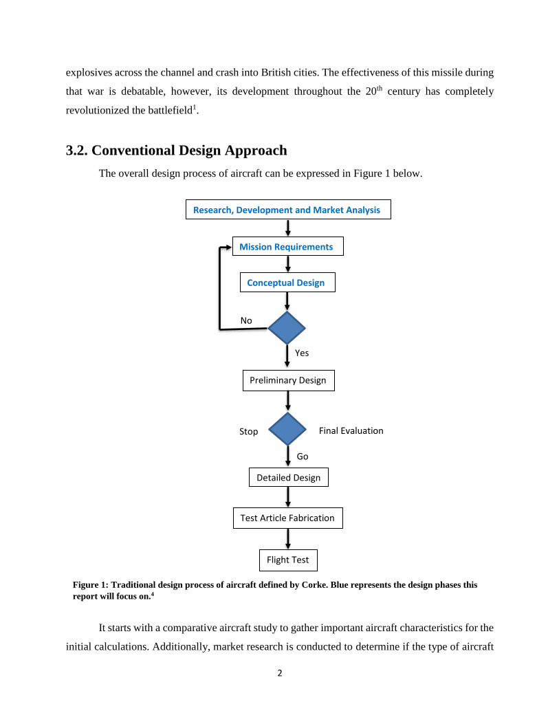
The overall design process of aircraft can be expressed in Figure 1 below.

It starts with a comparative aircraft study to gather important aircraft characteristics for the

initial calculations. Additionally, market research is conducted to determine if the type of aircraft

No

Research, Development and Market Analysis

Mission Requirements

Conceptual Design

Preliminary Design

Final Evaluation Stop

Detailed Design

Go

Test Article Fabrication

Yes

Flight Test

Figure 1: Traditional design process of aircraft defined by Corke. Blue represents the design phases this

report will focus on.4

3

the user wishes to develop is economically feasible. The next step is to define the type of mission

this aircraft will carry out. The aircraft may solely conduct aerial reconnaissance for military

applications, transport cargo/people domestically/internationally or the aircraft may be available

to civilians for recreational use only. Defining the mission will lead to defining design constraints,

with some tolerance, such as takeoff/landing distance, range, endurance, cruise altitude and so on.

The next step is to move into the conceptual design phase of the aircraft by calculating design

variables such as TOGW, L/Dmax, AR etc. while attempting to hold the design constraints constant.

As seen in Figure 1 above, this is an iterative process as the design constraints defined in the

mission requirements may have to be adjusted. The next phase is the preliminary design which

will focus on creating a basic proof of concept. This will involve performing calculations focused

around flight mechanics, structure stresses and stability and control calculations. At the conclusion

of this step, a design review is performed to ensure the current design is feasible practically and

economically. After the review has passed, the detailed design process will then focus on specific

components of the aircraft such as the tail design, propulsion system, landing gear, control

surfaces, equipment and subsystems and testing the integration between all these components.

Wind tunnel testing and CFD is also done at this stage. The final stage is the flight testing were

test pilots and a team of engineers will conduct a series of maneuvers to define the flight envelope

and to make sure the aircraft will successfully perform its overall mission4.

3.3. Cluster Computing

3.3.1 Moore’s Law

Explosion in the development of supercomputers and their uses by hobbyist, students,

universities etc. can be heavily contributed to the dramatic price drop of these awesome machines

due to Moore’s law. Moore’s law, developed by Gordon Moore in 1965, states that the number of

transistors per silicon chip will double every year17. Figure 2 below illustrates the advancement.

4

This law still roughly stands as it slowed down from 12 to 18 months. However, this law is

expected to continue throughout the 21st century as the size of transistors continues to shrink and

with their advancements such as the development of the 3D transistor17. The results from this law

can be linked to the drop-in cost of computing and the availability of computing power to

researchers with a lack of funding.

3.3.2. Aircraft Design and Supercomputers

Designing aircraft using supercomputers is not a new concept: universities, aircraft

industries and government agencies such as NASA are currently using supercomputers to generate

and test new designs of aircraft. Boeing purchased the global supercomputer leader, Cray Inc., and

utilized its processing power of billions of operations per second to build the very successful 787

Dreamliner5. NASA is currently using a supercomputer to help improve propulsion designs. A

team of engineers are using supercomputers to develop a radical new wing to cut down on weight

which can save the airline industry millions of gallons of fuel per year. A team of engineers used

this supercomputer to redevelop the wing of a Boeing 777 that weighed 5% less. These are just

some examples how supercomputers are utilized by Aerospace Engineers to solve the complex

problem of optimizing aircraft design19.

Figure 2: Advancement of the computer through time as it relates to transistor17

count[ref]

5

4. Methodology

4.1. Process of Conceptual Design

In order to accurately carry out multiple calculations at once, an iterative process is used.

The process begins with the selection of the user defined design constraints as stated in the above

section. The user will be able to select the desired range, endurance, cruise velocity and payload

weight. These design constraints can be seen in Table 1 below.

Endurance (E)

Range (R)

Cruise Alt. (Vcrs)

Payload Weight (Wp)

A comparative aircraft study is then conducted to establish a jumping-off point by using

the performance characteristics for initial calculations. Such characteristics as structural factor,

wing span, lift over drag ratio are just some that are utilized. Once design constraints are chosen

and structural factor and lift over drag ratio are estimated an initial aspect ratio, wing loading and

cruise altitude are chosen.

From these inputs and the design constraints, a gross takeoff weight is calculated using the

fuel fraction method. Once takeoff weight is determined, the specific structural weights are

calculated as well as the aerodynamic performance of the aircraft using general design methods

and a computer aided design of the fuselage and tail sections. Upon completion of the structural

and aerodynamic calculations, the values of lift to drag ratio and structural factor are reviewed in

comparison to initial estimates. If these values do not match, the initial values are altered, and the

above analysis is repeated yielding a new design. This process is continued until the initial estimate

of lift to drag ratio and structural factor (termination criteria) match the final calculations of those

parameters. Once values of structural factor and lift to drag ratio converge, the aerodynamic data

yields a required power loading.

With an initial design using a specified wing loading, aspect ratio and cruise altitude are

created and finalized, the wing loading is altered, and the above process is repeated for that new

wing loading. This process is done for wing loadings varying from ten to forty in increments of

Table 1: User defined design constraints

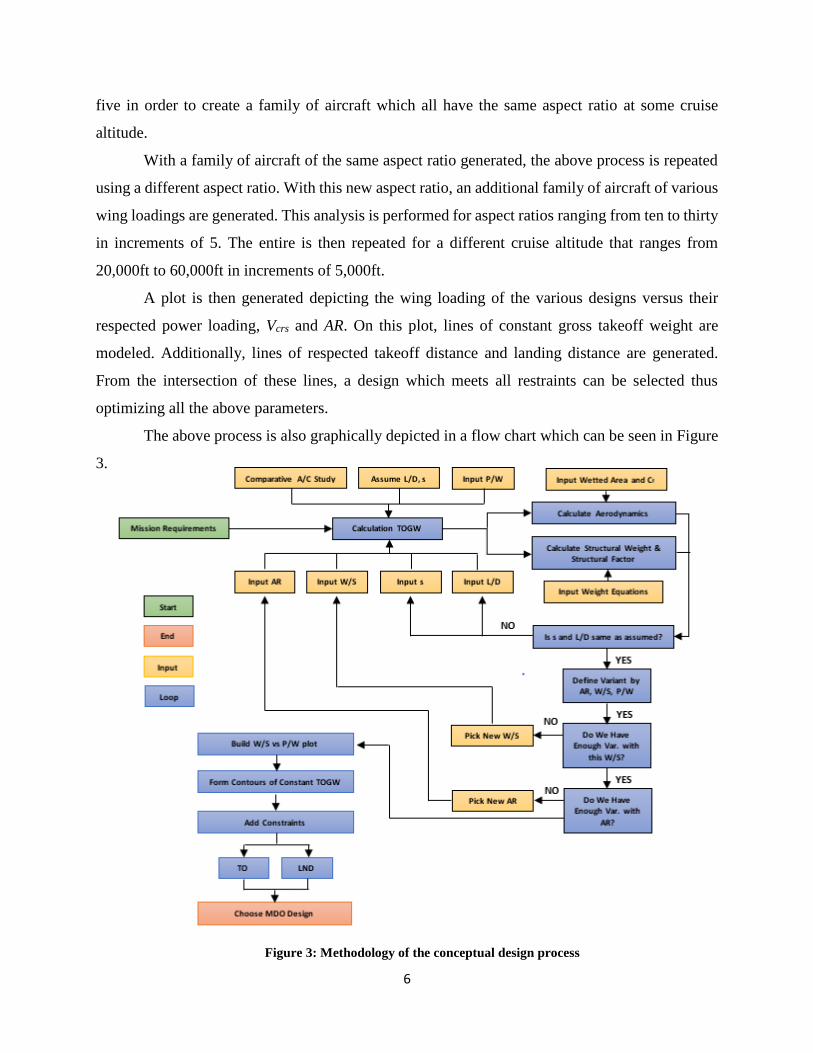
6

Figure 3: Methodology of the conceptual design process

five in order to create a family of aircraft which all have the same aspect ratio at some cruise

altitude.

With a family of aircraft of the same aspect ratio generated, the above process is repeated

using a different aspect ratio. With this new aspect ratio, an additional family of aircraft of various

wing loadings are generated. This analysis is performed for aspect ratios ranging from ten to thirty

in increments of 5. The entire is then repeated for a different cruise altitude that ranges from

20,000ft to 60,000ft in increments of 5,000ft.

A plot is then generated depicting the wing loading of the various designs versus their

respected power loading, Vcrs and AR. On this plot, lines of constant gross takeoff weight are

modeled. Additionally, lines of respected takeoff distance and landing distance are generated.

From the intersection of these lines, a design which meets all restraints can be selected thus

optimizing all the above parameters.

The above process is also graphically depicted in a flow chart which can be seen in Figure

3.

7

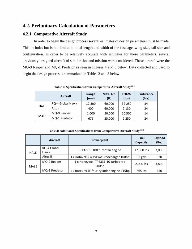
4.2. Preliminary Calculation of Parameters

4.2.1. Comparative Aircraft Study

In order to begin the design process several estimates of design parameters must be made.

This includes but is not limited to total length and width of the fuselage, wing size, tail size and

configuration. In order to be relatively accurate with estimates for these parameters, several

previously designed aircraft of similar size and mission were considered. These aircraft were the

MQ-9 Reaper and MQ-1 Predator as seen in Figures 4 and 5 below. Data collected and used to

begin the design process is summarized in Tables 2 and 3 below.

Aircraft Range (nmi)

Max. Alt. (ft)

TOGW (lbs)

Endurance (hrs)

HALE RQ-4 Global Hawk 12,300 60,000 32,250 34

Altus II 400 60,000 2,130 24

MALE MQ-9 Reaper 1,000 50,000 10,500 14

MQ-1 Predator 675 25,000 2,250 24

Aircraft Powerplant Fuel

Capacity Payload

(lbs)

HALE

RQ-4 Global Hawk

F-137-RR-100 turbofan engine 17,300 lbs 3,000

Altus II 1 x Rotax 912 4-cyl w/turbocharger 100hp 92 gals 330

MALE

MQ-9 Reaper 1 x Honeywell TPE331-10 turboprop 900hp

2,000 lbs 3,800

MQ-1 Predator 1 x Rotex 914F four-cylinder engine 115hp 665 lbs 450

Table 2: Specifications from Comparative Aircraft Study11,12

Table 3: Additional Specifications from Comparative Aircraft Study11,12

8

Due to the classification of these aircraft, most of their characteristics are not available to

the general public. As a result, rough estimates had to be made in some circumstances. In other

circumstances, such as the Swet, the fuselage was recreated in a computer aided design program

that was able to provide such a value. Please refer to Appendix A, Figures 21 and 22 for a depiction

of the CAD models of the MQ-1 Predator and MQ-9 Reaper.

4.2.2. Engine Study

A comparative study was conducted for dozens of Lycoming and Continental engines. The

different types of engines consisted of mainly turbocharged engines. A turbocharged engine uses

a turbine for forced induction. Dozens of engines were collected along with their specifications.

The power of the Lycoming and Continental engines were plotted against their weights to later

determine the most efficient engine based on the power needed for the aircraft and its lowest dry

weight. Figure 6 below represents all the Lycoming and Continental turbocharged engines. The

linear best fit line was also added. Please refer to Appendix C for specifications collected on all

the analyzed engines.

Figure 4: General Atomics’ MQ-1 Predator 11 Figure 5: General Atomics’ MQ-9 Reaper12

9

150

200

250

300

350

400

250 300 350 400 450 500 550 600

Po

wer

[H

P]

Dry Weight [lbs]

Lycoming Engines

Continental Engines

(𝐿

𝐷)

𝑚𝑎𝑥=

1

2√

𝜋 𝐴𝑅 𝑒

𝐶𝐷0

𝐶𝐿(

𝐿𝐷

)𝑚𝑎𝑥

= √𝜋 𝐴𝑅 𝑒 𝐶𝐷0

4.2.3. Initialization of Take-Off Gross Weight

In order to make initial calculations, estimates must be made of some key parameters to

serve as a “jump-off” point. In this manner, the estimated parameters can be continuously refined

to produce the best final result. For the purposes of this process, the parameters that are to be

initially estimated are the zero-lift drag coefficient, structural factor, and cruise lift-to-drag ratio.

With these preliminary estimates completed, it is then possible to calculate early

aerodynamic parameters, which will allow for the calculation of the takeoff gross weight. Several

such parameters are found via Equations 4.1, 4.2, and 4.3 below.

(4.1)

(4.2)

Figure 6: Weight as a function of power for turbocharged engines3

10

𝑉ℎ𝑜𝑙𝑑 =√

(𝑊/𝑆𝑟)

12 𝜌 𝐶𝐿

(𝐿𝐷)

𝑚𝑎𝑥

(4.3)

The fuel fraction method is the technique used to estimate the aircraft takeoff gross weight.

It involves estimating the relative amount of fuel an aircraft will use during a mission. It describes

the change in weight an aircraft experiences when it consumes fuel during a given phase of flight.

The distinct phases of flight are as follows for this computer program.

1) Start-up, Taxi, Run-up, Takeoff

2) Climb/Accelerate

3) Cruise

4) Loiter

5) Cruise

6) Holding or Reserve

7) Decent/Landing

For the first, second, and seventh phases of flight, simple ratios are used to determine the

fuel required for each of the phases. For example, it is estimated that the aircraft exits the first

phase of flight with 98% of the weight with which it entered that phase--that is, the aircraft

becomes 2% lighter due to fuel consumption.

For the third and fifth phases of flight, a more complex relationship is used. This

relationship relies on the Breguet Range Factor. The Breguet Range Factor encompasses the

Figure 7: Mission outline used for the fuel fraction in the computer program

11

𝑊𝑓𝑖𝑛𝑎𝑙 = (1 −1

𝑒𝑅

𝐵𝑅𝐹

) 𝑊𝑖𝑛𝑖𝑡𝑖𝑎𝑙

𝑊𝑓𝑖𝑛𝑎𝑙 = (1 −1

𝑒𝐸

𝐵𝐸𝐹

) 𝑊𝑖𝑛𝑖𝑡𝑖𝑎𝑙

𝑠 =𝑊𝑠𝑡𝑟

𝑊𝑇𝑂

𝑞 =1

2𝜌𝑉2

efficiency of the propeller, the cruise lift-to-drag ratio, and the specific fuel consumption of the

engine, in order to produce a value that reflects the aircraft’s relative range. It is calculated via the

following equation:

(4.4)

The fourth phase of flight also uses a special relationship that uses a quantity known as the

Breguet Endurance Factor. This factor includes the maximum lift-to-drag ratio, the specific fuel

consumption of the engine, and the holding velocity in order to give a value that shows the

aircraft’s relative endurance. Equation 4.5 shows this relationship below.

(4.5)

Evaluating each phase of flight from first to last gives an estimate of the comparative fuel

weight the aircraft must be able to accommodate. The takeoff gross weight is found based on the

selected structural factor, as shown below in Equation 4.6, which compares the required structural

weight to the overall takeoff gross weight.

(4.6)

Next, additional aerodynamic and geometric characteristics may be determined after the

calculation of dynamic pressure using Equation 4.7.

(4.7)

12

𝑆𝑟 =𝑊𝑇𝑂

(𝑊𝑆 )

𝑏 = √𝐴𝑅

𝑆𝑟

𝑐𝑟 =2𝑏

𝐴𝑅(1 + 𝜆)

𝑚𝑎𝑐 =2

3𝑐𝑟

(1 + 𝜆 + 𝜆2)

(1 + 𝜆)

𝑆𝑤𝑤𝑖𝑛𝑔= 2.03𝑆𝑟

𝑆𝑤𝑉𝑇= 𝑐𝑉𝑇

𝑏 𝑆𝑟

𝑙𝑉𝑇

𝑆𝑤𝐻𝑇= 𝑐𝐻𝑇

𝑚𝑎𝑐 𝑆𝑟

𝑙𝐻𝑇

4.2.4. Calculation of Aerodynamics

Using some key assumptions about the layout of the aircraft and general shape of the wing,

it is possible to find several geometric parameters, Equations 4.8, 4.9, 4.10 and 4.11, pivotal in

calculating aerodynamic characteristics:

(4.8)

(4.9)

(4.10)

(4.11)

Calculation of the zero-lift drag on the aircraft is accomplished using the wetted areas of

the aircraft components. These wetted areas are calculated in Equations 4.12, 4.13, 4.14, and 4.15.

(4.12)

(4.13)

(4.14)

13

𝑆𝑤 = 𝑆𝑤𝑤𝑖𝑛𝑔+ 𝑆𝑤𝑓𝑢𝑠

+ 𝑆𝑤𝑉𝑇+ 𝑆𝑤𝐻𝑇

𝐶𝐷0=

𝑐𝑓 𝑆𝑤

𝑆𝑟𝐹𝑄

𝐶𝐷0= 𝐶𝐷0𝑤𝑖𝑛𝑔

+ 𝐶𝐷0𝑓𝑢𝑠+ 𝐶𝐷0𝑉𝑇

+ 𝐶𝐷0𝐻𝑇

𝐶𝐿𝑐𝑟𝑠=

(𝑊𝑆𝑟

)

𝑞

𝐶𝐷𝑐𝑟𝑠= 𝐶𝐷0

+𝐶𝐿𝑐𝑟𝑠

2

𝜋 𝐴𝑅 𝑒

(4.15)

The wetted area of the fuselage was calculated from a design created in CAD program as

explained above. Given the wetted areas of aircraft components, calculating the total zero-lift drag

is no more than finding the effect of each component and adding them together, seen in Equation

4.16.

(4.16)

(4.17)

The coefficient of lift at cruise flight condition is calculated using Equation 4.18 below.

(4.18)

The coefficient of drag at cruise flight condition is simply the sum of the zero-lift drag

coefficient and the induced drag at cruise. It is calculated via Equation 4.19 below.

(4.19)

Using the normalized coefficient of lift, found in Equation 4.20, it is possible to recalculate

the previously-estimated cruise lift-to-drag ratio.

14

𝐶𝐿 =𝐶𝐿𝑐𝑟𝑠

𝐶𝐿(

𝐿𝐷

)𝑚𝑎𝑥

(𝐿

𝐷)

𝑐𝑟𝑠=

2𝐶𝐿 (𝐿𝐷)

𝑚𝑎𝑥

1 + 𝐶𝐿

2

𝑃𝑟𝑒𝑞 =1

550 𝑉𝑐𝑟𝑠

𝜂𝑝 [

𝑊𝐶𝐷0𝑞

(𝑊𝑆𝑟

)+ (

𝑊

𝑆𝑟)

𝑊

𝑞 𝜋 𝐴𝑅 𝑒]

𝑊𝑤𝑖𝑛𝑔 = 0.036𝑆𝑤0.758𝑊𝑓𝑤

0.0035 (𝐴

𝑐𝑜𝑠2𝛬)

0.6

𝑞0.006𝜆0.04 (100 𝑡

𝑐⁄

𝑐𝑜𝑠𝛬)

−0.3

(𝑁𝑧𝑊𝑑𝑔)0.49

𝑊ℎ𝑜𝑟𝑖𝑧𝑜𝑛𝑡𝑎𝑙𝑡𝑎𝑖𝑙

= 0.016(𝑁𝑧𝑊𝑑𝑔)0.414

𝑞0.168𝑆ℎ𝑡0.896 (

100 𝑡𝑐⁄

𝑐𝑜𝑠𝛬)

−0.12

(𝐴

𝑐𝑜𝑠2𝛬ℎ𝑡)

0.043

𝜆ℎ−0.02

𝑊𝑣𝑒𝑟𝑡𝑖𝑐𝑎𝑙𝑡𝑎𝑖𝑙

= 0.073 (1 + 0.2𝐻𝑡

𝐻𝑣

) (𝑁𝑧𝑊𝑑𝑔)0.376

𝑞0.122𝑆𝑣𝑡0.873 (

100 𝑡𝑐⁄

𝑐𝑜𝑠𝛬𝑣𝑡

)

−0.49

(𝐴

𝑐𝑜𝑠2𝛬𝑣𝑡

)0.357

𝜆𝑣𝑡0.039

(4.20)

(4.21)

Next, the power required to sustain flight at cruise is determined, shown below in Equation

4.22.

(4.22)

4.2.5. Calculation of Weights

Using Daniel Raymer’s general aviation equations for component weights, it is possible to

again calculate the total aircraft weight. The weight of the wing, horizontal tail, vertical tail and

fuselage were calculated using the equations represented as Equation 4.23, 4.24, 4.25 and 4.26

below.

(4.23)

(4.24)

(4.25)

15

𝑊𝑓𝑢𝑠𝑒𝑙𝑎𝑔𝑒 = 0.052𝑆𝑓1.086(𝑁𝑧𝑊𝑑𝑔)

0.177𝐿𝑡

−0.051(𝐿𝐷⁄ )

−0.072𝑞0.241 + 𝑊𝑝𝑟𝑒𝑠𝑠

(4.26)

With this sum of these weights, structural factor can be recalculated as well. It is imperative

that the estimated values of structural factor and cruise lift-to-drag ratio from the beginning of the

process match their calculated values after the estimation of takeoff gross weight and calculation

of aerodynamic parameters.

4.2.6. TOGW Analysis

In order to visualize the effects of gross weight on the performance characteristics of an

aircraft, lines of constant gross weight were plotted on the power loading and wing loading graph

which correspond to each aircraft variant. Using linear interpolation of the aircraft variant,

respective power loading and wing loading values where found from which lines where plotted.

These lines prove useful in later analysis as the lightest aircraft which satisfies a series of

constraints can be identified. Examples of these lines can be seen in Figures 8 and 9 below.

Figure 8: Constant TOGW lines at an altitude of 20,000ft

16

4.2.7. Design Constraint Analysis

4.2.7.1. Takeoff Distance

Takeoff distance can be resolved as a function of an aircraft’s power loading, wing loading,

and stall speed. Stall speed depends on the sizing of the wing and the airfoil selection. Airfoil

selection will be held constant with a NACA 23015 airfoil. For this analysis takeoff distance will

be modeled as the ground roll distance in which the aircraft accelerates to 1.2 times the stall speed,

a typical rotation speed. The obstacle distance is designated at 50 ft.

Factors which are held constant in this analysis but pertain to take off distance include prop

efficiency, lift curve slope, wing incidence angle, zero lift angle of attack, flap deflection, Oswald

efficiency factor, maximum lift coefficient, and finally zero lift drag.

Prop efficiency was selected to be held at a constant value of 86 percent, similar to that of

comparative aircraft. Lift curve slope for the NACA 23015 airfoil is 0.09, zero lift angle of attack

is negative one degree, and maximum lift coefficient is 1.6. These values are found from the

Theory of Wing Sections. Wing incidence angle was selected to be 1 degree which is similar to

the comparative aircraft. A fowler flap was used via comparative aircraft analysis which added a

base drag of 0.032. Oswald efficiency factor is selected to be 0.85 corresponding to the wings taper

Figure 9: Constant TOGW lines at an altitude of 25,000ft

17

𝑇𝑠𝑡𝑎𝑡𝑖𝑐 = (𝑃 𝜂𝑝550√2𝜌𝐴𝑑)2/3

ratio. Zero lift drag remains the same as in previous analysis with an increase of 0.025 for gear

deflection. The above parameters are summarized in Table 4 below.

Modeling of takeoff distance ground roll is a relatively simple analysis using basic physics

to model acceleration, velocity, and displacement. Using excel, a time vector is created with

increasing time by a selected increment.

The numerical integration used to calculate the takeoff length is a function of this time step

(Δt), acceleration of the aircraft in the x direction, magnitude of velocity along with its components,

thrust, lift, drag, friction, pitch, angle of attack and flight path angle. At t = 0 seconds, the velocity,

Sx, and angle of attack of the aircraft are all at equal to zero. However, there is static thrust from

the engines. This was calculated using Equation 4.27 below.

(4.27)

The effective angle of attack was then calculated. This is represented by Equation 4.28

below.

Aerodynamics

e 0.85

CLα (deg-1) 0.09

iw(deg) 1

α0L (deg) -1

δflaps (deg) 0

ηprop 0.86

ΔCD,flaps 0.032

ΔCD,gear 0.0250

CD0 0.0167

CL,max 1.6

Table 4: Aerodynamic Parameters

18

𝛼𝑒𝑓𝑓 = (𝜃 − 𝛾 + 𝑖𝑤 − 𝛼0𝐿 + ∆𝛼𝑓)

𝐴𝑅𝐺𝐸 =𝐴𝑅

√2ℎ𝑏

𝐶𝐷 = 𝐶𝐷0 +𝐶𝐿

𝜋 𝐴𝑅 𝑒+ ∆𝐶𝐷𝑔𝑒𝑎𝑟 + ∆𝐶𝐷𝑓𝑙𝑎𝑝

(4.28)

Effective angle of attack is a non-zero parameter at these static conditions because there is

incidence on the wing and is has a zero-lift angle of attack due to its airfoil properties. The effective

aspect ratio in ground effect was then calculated using Equation 4.29 below.

(4.29)

The coefficient of drag was then calculated using Equation 4.30 below. The extra terms

represent the change in drag due to the flaps and the landing gear on the aircraft as previously

mentioned.

(4.30)

The coefficient of drag can then be used to calculate the drag of the aircraft along with its

components. Equation 4.31 represents the drag of the aircraft. At t = 0, this value will be zero

because there is no dynamic pressure term. Due to the drag being zero, the drag components will

also go to zero at this moment. The drag components in the x can be represented by Equation 4.32

below.

(4.31)

𝐷 = 𝐶𝐷 𝑞 𝑆𝑟

19

(4.32)

The rolling friction force for the aircraft is now calculated using Equation 4.33 below. This

force decreases slightly as the aircraft makes its way down the runway due to lift increasing with

velocity. After the rolling phase ends and the aircraft is airborne, this value goes directly to zero.

(4.33)

The x-component of acceleration of the aircraft is finally solved using Equations 4.34

below. There is no acceleration in the y-direction until the aircraft is pitched upwards which creates

a velocity and acceleration vector in the y-direction which is not included in this analysis.

(4.34)

After the acceleration component is calculated, the integration process begins. The velocity

in the x-direction is then calculated using Equation 4.35 below. This equation uses the acceleration

calculated in the last time step. This is repeated for every time step.

(4.35)

The distance in the x-direction was then calculated using Equation 4.36 below. This

equation also depends on the acceleration component from the previous time step.

𝐷𝑥 = 𝐷 𝑐𝑜𝑠(ϒ)

𝐹𝑓 = 𝜇(𝑊 − 𝐿)

𝑎𝑥 =𝑔

𝑤(𝑇𝑥 − 𝐿𝑥 − 𝐷𝑥 − 𝐹𝑓)

𝑉1𝑥 = 𝑉0𝑥 + 𝑎𝑥∆𝑡

20

(4.36)

Using the velocity and distance components for this current time step, the lift, drag, friction,

thrust and acceleration are calculated again. This process is repeated at time step intervals of 0.5

seconds and until 1.2 times the stall speed in the x-direction is reached. Please refer to Appendix

C for the spreadsheet layout for the takeoff performance.

4.2.7.2. Landing Distance

In order to model the full landing process of the aircraft, four segments including approach,

translation, free roll, and braking were calculated independently. Approach landing distance was

calculated using Equation 4.37.

(4.37)

Translation distance was determined using Equation 4.38.

(4.38)

Both translation and approach distances are dependent on the radius of transition, RTR, and

height of transition, hTR, and as seen in Equations 4.39 and 4.40 means that these distances are

primarily dependent on the stall speed of the aircraft.

(4.39)

𝑆1𝑥 = 𝑆0𝑥 +𝑉1𝑥

2 − 𝑉0𝑥2

2𝑎𝑥

𝑆𝐴 =50 − ℎ𝑇𝑅

tan 𝛾

ℎ𝑇𝑅 = 𝑅𝑇𝑅 − 𝑅𝑇𝑅 cos 𝛾

𝑆𝑇𝑅 = 𝑅𝑇𝑅 sin 𝛾

21

(4.40)

The free roll segment is directly related to the stall speed of the aircraft in the landing

configuration, as seen in Equation 4.41.

(4.41)

The braking distance was determined using an iterative process. Using a time step of a half

second, starting at the landing configuration stall speed the lift, friction, and drag forces acting on

the aircraft are calculated at that time step and used to find the deceleration that is acting on the

aircraft. From that acceleration using the basic trajectory equations, the velocity at the next time

step and distance traveled are calculated.

By setting the total summation of landing distance to be 2,000ft, holding power loading

constant and solving for wing loading, a constraint line can be plotted on the original wing loading

and power loading plot. Please refer to Appendix C for the spreadsheet of the landing used to

calculate the landing performance

4.3. Cluster Computer

The development of the cluster computer stemmed from an efficiency issue that arose

during the calculation of the wing weight using the analytical approach. The approach involved

calculating the structural stresses the wing would encounter during flight and sizing the spars, ribs

and strings accordingly. This is usually done in the preliminary design phase, however, to achieve

a more accuracy in the structural factor calculation in the entire iteration process, this method was

originally employed. The entire iterative method involved matching cycling through AR, W/S and

cruise altitudes and matching the s and L/Dcrs from the previous iteration to the current iteration as

explained in the above sections. This can involve thousands of iterations and due to the nature of

intensity of the analytical method, the computational time rises from minutes to days. To combat

𝑆𝐹𝑅 = 3 (1.15 𝑉𝑆0)

𝑅𝑇𝑅 =(1.23𝑉𝑠0

)2

0.23𝑔

22

this, a supercomputer can be employed to distribute the workload to decrease this time. Without

the proper funding and access to already established supercomputers, a new inexpensive was

developed by creating a cluster computer made up of cheap Raspberry PIs. Figure 10 below shows

a CAD model of the cluster computer.

In order to distribute the workload across all the PIs, a new an architecture had to be

developed to be able accept jobs from MATLAB, compute the results and send back. As it

currently stands, MATLAB is not currently compatible to run standalone applications on a

Raspberry PI. A workaround was to redevelop the code into Python that would be able to accept

inputs fed from MATLAB, perform the calculations and output the results to a .mat file that

MATLAB can easily read. The information can be transferred across a high bandwidth network,

to achieve the lowest latency. Figure 11 below represents the flow of information throughout the

cluster computer.

Figure 10: CAD model of the cluster

computer

23

This method to decrease computational time was successful, however, the analytical

method of calculating the weight of the wing was scratched from this report and will be revised in

future developments of this program. The cluster computer was still able to decrease the

computational time by distributing jobs for calculating the fuel fraction method within the total

iterative process.

4.4. Verification and Validation

Every computer program created must pass through the four main testing stages in order

to be fully validated before its release. These testing stages are shown in Figure 12 below.

Unit Testing represents the first stage, and this involves extensive testing of each

component of the product. As an example, if one were to build a computer, each component such

as the motherboard, power supply, optical drive etc. should be tested individually. The fuel fraction

method, aerodynamic calculations, Raymers weight calculations, the calculation of the structural

factor are all seen as individual units. The next testing stage, Integration Testing, involves the

testing of how the different units work together. Using the computer building example, one would

.

.

.

8 Raspberry PIs

LAN Network

Figure 11: Flowchart representing the workflow through the cluster computer

Unit Testing Integration

Testing System

Testing Acceptance

Testing

Figure 12: Four levels of software testing

24

want to verify that the motherboard receives power from the power supply and the CPU and RAM

are fully integrated with the motherboard. The fuel fraction method must produce a TOGW that

the power required equation uses to determine the W/P and the s is calculated from the summation

of the weight equations and so on. These previous two testing stages fall under term verification.

The next stage, System Testing, involves using a team of independent testers, using multiple

different testing schemes, to determine if the final product is producing results that fall under the

requirements that were laid out by the developers. The testers would determine if the PC, one is

building, can turn on, turn off, open the CMD prompt, execute commands etc. The developer for

this computer program created specific requirements such as the program must be able to allow

the user to input design constraints, the program should be able to calculate the lowest the most

efficient aircraft, lowest TOGW that fall within these constraints and the program should output

these results to readable text file for further analysis by the user. The last testing stage is the

Acceptance Testing. This involves allowing the user to test the final product to determine if it is

acceptable before distribution. These last two testing stages fall under validation. This computer

program currently is in Integration Testing stage.

During the integration testing, one of the testing schemes was designed to determine the

bounds of the user defined design constraints of this program. After analysis of the equations used,

it was determined that these constraints have a coupled relationship. The user would not be able to

change one constraint without it affecting another. The question is, what are the bounds of the

constraints in this methodology? Dozens of the runs were conducted to roughly determine the

limits of the user. Figure 13 and 14 below represents these results.

0 < 𝑅 < 1000 [𝑛𝑚𝑖]

0 < 𝐸 < 15 [ℎ𝑟𝑠]

50 < 𝑉𝑐 < 300 [𝑘𝑡𝑠]

200 < 𝑊𝑝 < 3000 [𝑙𝑏𝑠]

Figure 13: Limits of the design constraints from regression testing

25

5. Results and Discussion

Several aircraft design simulations were conducted in the testing of this program. Two of

these simulations will be discussed in this section. The first run used a range of 650nmi, endurance

of 10hrs, cruise velocity of 200kts and a payload weight of 2,000lbs. A 3d plot representing the

iterative solution is shown in Figure 15 below.

Figure 14: Boundary testing results of the user defined design constraints

Figure 15: Variant results with design constraints of R = 650nmi, E = 10hrs, Vcrs = 200kts, Wpay = 2000lbs

26

This plot represents the family of aircraft that were generated at various AR, W/S and cruise

altitudes. The y-axis represents the W/P which is the TOGW over the power required. The TOGW

constants and TO and LND constraints were then added and represented in Figure 16 below.

The family of aircraft were split up into 2D plots for easier representation. At an altitude

of 30,000ft and 35,000ft it is interesting to note the 8,000lb TOGW line splits into two directions

when the AR is 10. This suggests at this AR, there are multiple designs with the same TOGW. These

results also suggest that there are no aircraft designs that have a TOGW less than 8,000lbs. There

are no aircraft that were produced to the right of the least constant TOGW line, which means this

is the least TOGW one can achieve with these design constraints. To the left of this, the TOGW

will only increase.

The landing and takeoff constraints must now be considered before choosing an aircraft.

The landing constraint, represented by the vertical black line, represents the W/S the aircraft must

have in order to achieve a landing distance of 2,000ft. As the W/S increases the takeoff distance

Figure 16: TOGW constants for R = 650nmi, E = 10hrs, Vcrs = 200kts, Wpay = 2,000 lbs

27

will increase, so only an aircraft to the left of this line will be considered. The takeoff constraint,

represented by the red line, represents the W/S and W/P the aircraft must have in order to takeoff

at a distance of 3,000ft. As the W/S increases the takeoff distance will increase, so only aircraft

that are to the left of this constraint can be considered. After considering these constraints, the

efficient aircraft can be chosen at every cruising altitude. At an altitude of 35,000ft the most

efficient design will be an AR of 25, W/S of 20lbs/ft2 with a TOGW of around 9,000lbs. The same

method of choosing the efficient design can be applied to every cruising altitude. This

methodology was applied to an altitude of up to 60,000ft, however, only MALE UAVS are

considered in this report. If one wanted to design a HALE (high altitude long endurance) UAV the

aircraft characteristics would have to be altered inside the program to reflect a comparative aircraft

such as the MQ-4 Triton. The design constraints would also be changed to reflect a HALE UAV.

The second run that was conducted had a range of 250nmi, endurance of 15hrs, cruise

velocity of 150kts and a payload of 3,000lbs. Figure 17 below represented the family of aircraft

generated by the algorithm.

The run that was conducted considered the same range of design variables as the previous

run. Figure 18 below represent the same family of aircraft split up by cruising altitude with the

same takeoff and landing constraints plotted.

Figure 17: Variant results with design constraints of R = 250 nmi, E = 15 hrs, Vcrs = 150 kts, Wpay = 3,000 lbs

28

It is interesting to point out that there are no valid aircraft designs to choose from at

altitudes from 25,000ft – 35,000ft. Unfortunately, currently, the computer program is not capable

of detecting these instances and not capable of displaying a recommended design. The plotting of

the constant TOGW, LND and TO constraints and choosing the design had to be done manually in

Excel. However, future iterations of this program will be able to solve this data analytics issue.

Figure 18: TOGW constants for R = 250nmi, E = 15hrs, Vcrs = 150kts, Wpay = 3,000 lbs

29

6. Conclusion

This report highlights the methods used to create an efficient conceptual design system

capable of maximizing the efficiency of a MALE UAV. The conceptual design method, as

described in this report, yields several families of aircraft with various configurations which all

meet the design constraints imparted. These family of aircraft were then plotted individually on a

graph along with lines of constant gross weight along with lines representing additional constraints

such as takeoff and landing distance. From the final graphs, an efficient design configuration was

determined by finding an aircraft which falls between all constraints, and this aircraft represents

the most efficient design possible under the initial specifications from the beginning of the design.

As of today, this program contains the bedrock for efficient UAVs designs in the

conceptual stage. Several improvements will be made and will be discussed in detail in the next

section. The code is still considered static, in which it will crash if the constraints, set by the user,

are unacceptable. This was established through the limit testing stage. Again, this does not mean

an aircraft cannot be created with given these constraints, it means that the somewhere in the

iteration process, the calculated design variables would not allow the termination criteria to be

satisfied and caused a crash. This would have to be addressed in future developments. Lastly this

program needs to complete the final testing stages and receive validation before being released to

potential users.

30

7. Future Work

As it stands, this program should be seen as a foundation that has plenty of room to expand.

The code methodology can be refined to become more efficient with the increased integration of

the cluster computer. The current computing power from the is not being utilized to its fullest.

Parallel algorithms can be implemented inside the current program that can dispatch jobs to the

computer using a more advanced architectural design. Additionally, more cores can be added to

the computer with an additional purchase of eight Raspberry PIs. Currently the casing of the

computer was designed to hold sixteen PIs and currently only eight are installed.

The methodology itself also has room to expand. The code currently contains a database

of engines that the algorithm will select from to meet the power install requirement and have the

lowest dry weight. The database only contains turbocharged engines which can severely limit the

ability to have high cruising altitude. An addition of supercharged engines along with diesel grade

turbocharged and supercharges engines will further expand the algorithms capability to design a

high-altitude aircraft. Additionally, this is a static program. It lacks dynamic capability such as

recognizing dead designs. As the program iterates through and designs the family of aircraft, if it

comes across a specific AR, cruise altitude and W/S that will not produce a valid structural factor

and/or L/Dcrs, the program will terminate. The algorithm can be modified to recognize this as a

dead aircraft and move onto the next iteration.

Machine learning can also be introduced into the algorithm to guide the user into making

appropriate choices for the design constraints that are within the bounds of the algorithm. It was

discussed in the Results and Discussion section that the current algorithm places limits on what

the user can chose as the design constraints. The limits that were defined are based off only a

handful of tests. Machine learning code can be integrated into the current algorithm to further

refine these limits by running numerous design simulations.

Currently this algorithm is restricted to only the conceptual design phase. An expansion

into the preliminary design phase will allow the user to determine if the most efficient design is

feasible.

A full validation process is needed to determine is this methodology can produce accurate

results. This will involve the process of redesigning an already proven aircraft such as the MQ-9

and MQ-1 and determining if the design variables produced from the program come within a

certain tolerance of the actual design variables of these aircraft. Additionally, a test team will have

31

to preform regression testing on this product to determine if program is behaving as outlined in the

methodology.

32

References

1. “A Brief History of Aircraft Structures,” Aerospace Engineering Blog, 24-Jul-2018.

[Online]. Available: https://aerospaceengineeringblog.com/aircraft-structures/.

[Accessed: 02-Nov-2019].

2. “Cluster Computing: History, Applications and Benefits,” UKEssays.com. [Online].

Available: https://www.ukessays.com/essays/computer-science/cluster-computing-

history-applications-9597.php. [Accessed: 02-Nov-2019].

3. “Continental 500 Series AvGas Engine,” Continental Aerospace Technologies. [Online].

Available: https://www.continentalmotors.aero/engines/500.aspx. [Accessed: 27-Oct-

2018].

4. T. C. Corke, Design of aircraft. Singapore: Pearson Education, 2005.

5. “Cray Supercomputers Play Key Role in Designing Boeing 787 Dreamliner.” Cray Inc.

Accessed September 30, 2019. https://investors.cray.com/news-releases/news-release-

details/cray-supercomputers-play-key-role-designing-boeing-787.

6. Y. Domun, “Aircraft Design Process Overview,” EngineeringClicks, 06-Oct-2018.

[Online]. Available: https://www.engineeringclicks.com/aircraft-design-process/.

[Accessed: 20-Aug-2019].

7. B. Dunbar, “NASA Dryden Fact Sheet - ALTUS II,” NASA, 31-Mar-2015. [Online].

Available: https://www.nasa.gov/centers/armstrong/news/FactSheets/FS-058-

DFRC.html. [Accessed: 20-2019].

8. Peter Gall, Class Lecture, Benjamin Statler College of Engineering and Mineral

Resources, West Virginia University, Morgantown, W.V., Fall 2014.

9. L. George, “3D Transistor Intel Reinvents Transistors,” electroSome, 13-Nov-2014.

[Online]. Available: https://electrosome.com/3d-transistor/. [Accessed: 02-Nov-2019].

10. J. Gundlach, “Multi-Disciplinary Design Optimization of Subsonic Fixed-Wing

Unmanned Aerial Vehicles Projected Through 202,” dissertation, 2004.

11. “MQ-1B Predator,” U.S. Air Force, 23-Sep-2015. [Online]. Available:

https://www.af.mil/About-Us/Fact-Sheets/Display/Article/104469/mq-1b-predator/.

[Accessed: 02-Aug-2019].

12. “MQ-9 Reaper,” U.S. Air Force, 23-Sep-2015. [Online]. Available:

https://www.af.mil/About-Us/Fact-Sheets/Display/Article/104470/mq-9-reaper/.

[Accessed: 02-Jul-2018].

33

13. D. P. Raymer, Aircraft Design: a conceptual approach. Washington, D.C., 1992.

14. “RQ-4 Global Hawk,” U.S. Air Force, 27-Oct-2014. [Online]. Available:

https://www.af.mil/About-Us/Fact-Sheets/Display/Article/104516/rq-4-global-hawk/.

[Accessed: 15-Aug-2019].

15. T. Scheve, “How the MQ-9 Reaper Works,” HowStuffWorks Science, 25-Jul-2019.

[Online]. Available: https://science.howstuffworks.com/reaper1.htm. [Accessed: 28-Oct-

2019].

16. “Supercomputer redesign of aeroplane wing mirrors bird anatomy,” Nature News.

[Online]. Available: https://www.nature.com/news/supercomputer-redesign-of-aeroplane-

wing-mirrors-bird-anatomy-1.22759. [Accessed: 02-Nov-2019].

17. The Editors of Encyclopaedia Britannica, “Moore's law,” Encyclopædia Britannica, 29-

Mar-2019. [Online]. Available: https://www.britannica.com/technology/Moores-law.

[Accessed: 20-May-2019].

18. WagnerOct, “Watch a supercomputer design a radical new wing for airplanes,” Science,

27-Dec-2018. [Online]. Available: https://www.sciencemag.org/news/2017/10/watch-

supercomputer-design-radical-new-wing-airplanes. [Accessed: 02-Nov-2019].

19. B. Yirka, “A supercomputer tool that can optimize airplane wing design offers improved

detail,” Tech Xplore - Technology and Engineering news, 05-Oct-2017. [Online].

Available: https://techxplore.com/news/2017-10-supercomputer-tool-optimize-airplane-

wing.html. [Accessed: 02-Oct-2019].

34

Appendix A

Appendix A represents the CAD models that were developed to gather further

characteristics for the comparative aircraft study.

35

Figure 19: MQ-9 developed in CAD

Figure 20: MQ-1 developed in CAD

36

Appendix B

Appendix B represents GUIs created to ease the use of the computer program.

37

Figure 21: Convergence Data GUI

Figure 22: Resource Center GUI

38

Appendix C

Appendix C represents the Excel sheets that aided in the calculations as seen in

this report. It was cleaner to represent these tables in a CD that is available with

the author’s permission.