i

THE RELATIONSHIP BETWEEN El NIÑO SOUTHERN

OSCILLATION AND LEVELS OF PARALYTIC SHELLFISH

POISONING PRESENT IN WASHINGTONS MARINE WATERS

By

Randy N. Lumper

A Thesis: Essay of Distinction Submitted in partial fulfillment of the requirements for the degree Master of Environmental Study The Evergreen State College

June 2008

ii

This Thesis for the Master of Environmental Study Degree

by

Randy Lumper

has been approved for

The Evergreen State College

by

________________________ Member of the Faculty ________________________ Date

iii

2008 by Randy Lumper. All rights reserved.

i

THE RELATIONSHIP BETWEEN El NIÑO SOUTHERN OSCILLATION AND LEVELS OF PARALYTIC

SHELLFISH POISONING PRESENT IN WASHINGTONS MARINE WATERS.

Randy Lumper

Can large scale weather phenomenon such as El Nino Southern Oscillation be used to predict when levels of paralytic shellfish poisoning will be higher, thus mitigating their harmful impacts? This thesis examines the relationship between levels of Paralytic Shellfish Poisoning (P.S.P.) present in Washington State’s marine waters and large scale weather phenomena or Oceanic circulation patterns such as the El Niño Southern Oscillation (ENSO). It questions whether large scale climatic conditions such as those produced by ENSO affect blooms of algae, such as Alexandrium catenella. Once we have a better working knowledge of the ecology of A. catenella we can better predict and monitor outbreaks of P.S.P., thus reducing the amount of human illnesses and economic hardships associated with P.S.P. The P.S.P. data is compared to sea surface temperatures departures from the normal in Niño region 3.4, and localized weather parameters to see if any significant relationship exists. As indicated by the results of this study P.S.P. levels in Washington State are not influenced by the phases of ENSO.

iv

Table of Contents List of Figures ....................................................................................................... v List of Tables ....................................................................................................... vi Chapter 1 Introduction .......................................................................................... 1

1.1 Background and Problem Description .................................................... 2 1.2 Thesis Statement and Layout ................................................................. 5

Chapter 2 Paralytic Shellfish Poisoning and Alexandrium Catenella Life Cycle .... 7 2.1 The Life Cycle of Alexandrium Catenella and the Physical Processes of its Environment ................................................................................................ 10 2.2 Turbulence ............................................................................................ 14 2.3 Precipitation and Runoff ....................................................................... 17 2.4 Salinity .................................................................................................. 18 2.5 Water Temperature .............................................................................. 19

Chapter 3 Large Scale Oceanic Circulation Patterns Such as ENSO Affect Regional Weather, and Drive Small Scale Physical Processes .......................... 23

3.1 The El Niño Southern Oscillation (ENSO) ............................................ 23 3.2 La Niña ................................................................................................. 26 3.3 ENSO Influence on Pacific Northwest Climate and Weather ................ 27

Chapter 4 Climate Changes Impacts to Pacific Northwest Weather and ENSO . 30 Chapter 5 Data Sources ..................................................................................... 34

5.1 ENSO Index .......................................................................................... 34 5.2 WDOH Database .................................................................................. 35

Chapter 6 Analysis and Results .......................................................................... 40 6.1 Air temperature .......................................................................................... 47 6.2 Wind .......................................................................................................... 49 6.3 Precipitation ............................................................................................... 51 6.4 Multiple liner regression analysis ............................................................... 52

Chapter 7 Implications of This Study .................................................................. 57 7.1 Regulatory Agencies and/or Groups ..................................................... 59 7.2 Shellfish Industry .................................................................................. 60 7.3 Recreational Harvest and Tribal Ceremonial/Subsistence Harvesting . 63

Chapter 8 Conclusion ......................................................................................... 65 References: ........................................................................................................ 68

v

List of Figures Figure 1: Alexandrium catenella Photo: by Jan Rimes. ............................................. 1

Figure 2: The world wide distribution of P.S.P. during 1970 and 2000,Glibert 2005.................................................................................................................................... 3

Figure 3: Meroplanktonic life cycle of the dinoflagellate species Alexandrium (Anderson, 2005). ............................................................................................................ 9

Figure 4: Mean and anomalies of sea surface temperature (SST) from 1986 to present, showing El Niño events left 1986-1987, 1991-1992, 1993, 1994 and 1997 and La Niña events right in 1985 and 1995 (www.pmel.noaa.gov/tao/elNiño/la-Niña-story.html). ............................................... 25

Figure 5: a (left)-b (right): Box-and-whisker plots showing the influence of ENSO on October-March (a) temperature and (b) precipitation (1899-2000). For each plot, years are categorized as cool (La Niña), neutral (ENSO neutral), or warm (El Niño). For each climate category, the distribution of the variable is indicated as follows: range of values (whiskers); median value for the phase category (solid horizontal line); regional mean for all categories combined (dashed horizontal line); 75th and 25th percentiles (top and bottom of box). Area-averaged Climate Division data are used for temperature and precipitation (C.I.G., 2008). ................................................................................................................. 27

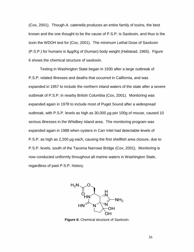
Figure 6: Chemical structure of Saxitoxin .................................................................. 36

Figure 7: ENSO over time based on a threshold of +/- 0.5ºC which is calculated from a 3 month running mean of sea surface temperature anomalies or “departures from normal” in the Niño 3.4 region which is based on the 1971-2000 base period. An El Niño or La Niña event occurs when the threshold of +/- 0.5ºC is met or exceeded for a minimum of 5 consecutive months. ................................. 41

Figure 8: P.S.P. levels for the period 1/1/1977-12/31/2007, over time .................. 41

Figure 9: P.S.P. levels equal to or less then 5,000µg STX/100g over time .......... 42

Figure 10: 3 month moving average of P.S.P. µg STX/100g levels over time ..... 43

Figure 11: Area plot of 3 month running means departures from normal for both ENSO and P.S.P. levels in Washington States marine waters. ............................. 44

Figure 12: Linear Regression of Log of 3 month moving average vs. ENSO Index........................................................................................................................................... 46

Figure 13: Linear Regression of Log of 3 month moving average vs. mean daily air temperature (C) ......................................................................................................... 49

Figure 14: Linear Regression of Log of 3 month moving average vs. max daily wind speed ...................................................................................................................... 49

Figure 15: Linear Regression of Log of 3 month moving average vs. average daily wind speed ............................................................................................................. 51

Figure 16: Linear Regression of Log of 3 month moving average vs. daily precipitation amount (inches) ....................................................................................... 52

Figure 17: Estimated West Coast production of farmed oysters, clams, mussels and geoduck, 2000 http://www.psat.wa.gov/Programs/shellfish/fact_sheets/economy_ web1.pdf. .... 58

vi

List of Tables Table 1: Multiple regression of the log of the 3 month moving average vs. the ENSO index, daily air temperature, max daily wind speed, daily wind speed, and daily precipitation ............................................................................................................ 53

Table 2: Correlation output among the Independent variables. .............................. 54

Table 3: Multiple regression of the log of the 3 month moving average vs. the ENSO index, daily air temperature, daily wind speed, and daily precipitation amounts. .......................................................................................................................... 55

Table 4: Multiple regression of the log of the 3 month moving average vs. the ENSO index, daily air temperature, and daily wind speed. ..................................... 56

1

Chapter 1

Introduction

Figure 1: Alexandrium catenella Photo: by Jan Rimes.

Millions of microscopic plant cells, commonly known as algae, thrive in

nearly every drop of seawater. Algae (phytoplankton) are the primary energy

producers in the ocean, forming the base of the marine food chain. These

single-celled plants photosynthesize and multiply, creating a bloom that feeds

everything from fellow microbes to larger fish species. Primary production is the

synthesis and storage of organic molecules during the growth and reproduction

of photosynthetic organisms such as algae. Seasonal phytoplankton dynamics

are most often characterized by low biomass and primary productivity during

winter-spring seasons of high river flow, followed by a slow (2-3 months)

accumulation of biomass during summer (Alpine, 1992). Typically during late

spring and early summer the dominate phytoplankton is diatoms, a species that

thrives in un-stratified environments and is unable to migrate below the

2

thermocline when nutrients become depleted in the surface layer. Once nutrients

become depleted in the surface layers, more motile species such as

dinoflagellates become dominate, due to their ability to migrate below the

thermocline and carry on photosynthesis when other algae are dying off. Among

the thousands of species of algae in the sea, a few dozen produce toxins and

pose a formidable natural hazard. In Washington’s Puget Sound basin the

dinoflagellate Alexandrium catenella (Figure 1) is one such species.

This thesis looks at the relationship between the dinoflagellate A. catenella

and the climate phenomenon know as El-Nino Southern Oscillation (ENSO).

ENSO, a global-scale weather phenomenon influences local climate, which in

turn influences the physical properties of the environment where A. catenella, is

found. This thesis asks the question, is there a relationship between the phases

of ENSO, and levels of paralytic shellfish poisoning present in Washington States

marine waters? If a relationship exists between the phases of ENSO or a

parameter of A. catenellas environment and the paralytic shellfish poisoning

levels produced by A. catenella, then ENSO can be used to predict when blooms

of Paralytic shellfish poisoning are likely to occur. If this is the case then

regulators of the shellfish industry may be able to use this information to mitigate

the economic and health impacts from blooms A. catenella and the paralytic

shellfish poisoning that it produces.

1.1 Background and Problem Description

3

Early records, partially based on local native lore passed down by word of

mouth, suggest that harmful algal blooms have been present along the coast of

the United States for hundreds of years (Trainer, 2003), but actual historic

scientific data are non-existent.

Figure 2: The world wide distribution of P.S.P. during 1970 and 2000, Glibert 2005.

“Historically, P.S.P. has been known in the Pacific Northwest and Alaska for centuries. Records of P.S.P. events date back as early as June 15, 1793 (Vancouver 1798), when a member of Captain George Vancouver’s exploration team died after eating contaminated mussels

4

harvested in the uncharted coastline of what is now known as British Columbia (Trainer, 2003)”.

Washington State’s only three fatalities due to paralytic shellfish poisoning were

recorded in 1942 near the entrance to the Strait of Juan de Fuca, since then

there has been no illnesses resulting in death.

Harmful algal blooms have been known throughout the world and

recorded history, but the nature of the problem has changed considerably over

the past several decades, both in extent (Figure 2) and in public perception.

Over the past three decades, the occurrence of harmful or toxic algal incidents

has increased in many parts of the world, both in frequency and in geographic

distribution (Van Dolah, 2000). This increase in occurrence and awarness has

public officials and citizens both calling for a greater scientific understanding of

the biological and physical properties associated with harmful algal blooms.

There are many theories to what sets the stage for large scale blooms of

A. catenella and other harmful algal blooms around the world.

“One cause for the increasing frequency of harmful algal blooms seems to be nutrient enrichment-that is, too much “food” for the algae. Just as the application of fertilizer to lawns can enhance grass growth, marine algae grow in response to nutrient inputs from domestic, agricultural, and industrial runoff (Anderson, 2004)”.

Though nutrient enrichment increases the amount of available food for A.

catenella and other harmful algal blooms, it does not necessarily allow the

blooms to persist for longer durations or increase the frequency of blooms inter-

annually. Recent studies suggests that not only do nutrients play a role, but that

physical process may be important in creating a favorable environment for large

scale blooms, and may be what is enabling blooms to persist in the environment

5

longer than historically recorded. Currently, not much is known about how

physical processes such as wind, precipitation, salinity, and water temperature,

limit or enhance the duration and frequency of harmful algal blooms. However, a

growing body of laboratory, field, and theoretical work suggests that the

dynamics of harmful algal blooms and their impacts on other organisms are

frequently controlled not only by physiological responses to local environmental

conditions as modified by trophic interactions, but also by a series of interactions

between biological and physical processes occurring over an extremely broad

range of temporal an spatial scales (Donaghay, 1997). Some of these physical

processes are not yet defined at the appropriate scale, yet may be crucial in the

formation of harmful blooms (Gentein, 2005). Physical factors affecting A.

catenella will be even harder to quantify in the future as we live in a world of

changing climate.

1.2 Thesis Statement and Layout

Do the phases of ENSO have an influence on paralytic shellfish poisoning

levels in Washington State? It is undetermined at this time if this is the case,

however, by performing statistical analysis of paralytic shellfish poisoning levels

in Washington States marine waters versus ENSO it may be possible to

determine if such a relationship exists.

The layout of this thesis was designed in the following order to provide a

logical path to answering the question above. The first two chapters break down

6

the life cycle of A. catenella, and how the physical properties of its environment

influence this life cycle. Chapter 3 looks at how the different phases of ENSO

affect local weather parameters and patterns, and thus the physical properties of

A. catenella environment. Chapter 4 discusses how climate change influences

ENSO and local weather. Chapter 5 describes the data sources used for this

study. Chapter 6 includes a statistical analysis of ENSO and associated weather

patterns versus paralytic shellfish poisoning levels in Washington State and the

results obtained from this analysis. The following chapter, Chapter 7, is a

discussion of what the implications of this study may have for individuals and

industries impacted by paralytic shellfish poisoning and those who regulate them.

Finally, Chapter 8 states the conclusions and discusses the implications that a

relationship between ENSO and paralytic shellfish poisoning levels in

Washington State may have and how this study may be strengthened in the

future.

7

Chapter 2

Paralytic Shellfish Poisoning and

Alexandrium Catenella Life Cycle

A. catenella is an armored, marine, planktonic dinoflagellate associated

with toxic Paralytic Shellfish Poisoning (P.S.P.). A. catenella occurs either as

single cells or as a chain of cells (Figure 1). A. catenella produces an array of

chemically similar neurotoxins that are responsible for P.S.P., which are

transmitted via tainted shellfish. Neurotoxins are so named because they disrupt

nerve impulses. P.S.P. toxin accumulates in marine animals that feed either

directly on toxic phytoplankton or on consumers of toxic phytoplankton. Bivalve

shellfish concentrate biotoxin’s when they filter toxic phytoplankton (A. catenella)

out of the water while feeding.

“These consumers include zooplankton, bivalve shellfish, predatory marine snails, crabs, fish, birds, and marine mammals. Mass mortalities among other shellfish-eating animals including birds, fur seals, foxes, sea otters, and humpback whales have been traced to P.S.P. (Determan, 2003)”.

These toxins can make their way up the food chain and end up affecting

humans, other mammals, fish and birds. On a global basis, almost 2,000 cases

of human poisonings are reported per year, with a 15% mortality rate (Van Dolah,

2000). “Human illness and death are the primary impact of Harmful algal

blooms, but effects on other wildlife are also important. Some fish kills due to

8

Harmful algal blooms can be spectacular is size, with millions of fish and millions

of dollars lost to local economies (Glibert, 2005)”. In the Puget Sound the

seasonal occurrence of A. catenella follows a scenario like this and the one in

Figure 3. Wintertime rain storms, rivers, and storm water runoff carry nutrients

into Puget Sound from uplands and watersheds. Strong winds mix the

freshwater with nutrient rich water from the open sea. Typically sunlight is the

most dominate factor limiting growth in the winter, however strong winds and

colder water temperatures may have an affect (Determan, 2003). In early spring,

winds become lighter reducing mixing, and the sun warms the water raising

water temperatures.

This causes the water column to stabilize and vertical mixing to slow down

or stop. A second influx of nutrients is then introduced in the form of snowmelt,

which increases the flow of most Puget Sound Rivers. The addition of these

abundant dissolved nutrients in a stable water column lead to blooms of many

phytoplankton species in the surface waters (Determan, 2003).

These blooms can be so dense that they can color the water red, brown,

green etc; this condition is called a “red tide”, and is often thought to be

associated with P.S.P., which is a common misconception. A. catenella may be

present in shellfish at dangerous levels, long before the water becomes

discolored (Determan, 2003). By mid to late summer, surface water is frequently

depleted of nutrients and many species of phytoplankton die back.

9

Figure 3: Meroplanktonic life cycle of the dinoflagellate species Alexandrium (Anderson, 2005).

However, two flagella enable A. catenella to vertically migrate to the

surface during the day and to depth at night. Because of this, A. catenella is able

to journey to deeper water via its flagella, where nutrients remain in abundance

(Trainer, 2003). Thus when nutrients become depleted at the surface during

summer A. catenella can simply move down to where nutrients are still

10

abundant, giving it an advantage over non-flagellated phytoplankton such as

diatoms. A. catenella then returns to the surface layer to carry on

photosynthesis. As a result of this A. catenella is able to bloom longer typically

until late autumn. At this time water temperatures begin to cool off and winds

speeds increase, inducing vertical mixing that leads to the breakdown of the

stratification of the water column, while sunlight starts to become too dim thus

limiting or shutting down the blooms production. At which time A. catenella may

form resting cysts that settle to the bottom awaiting the return of more favorable

growing conditions (Figure 3).

2.1 The Life Cycle of Alexandrium Catenella and the Physical

Processes of its Environment

The physical properties of aquatic environments play a fundamental role in

driving the dynamics of planktonic communities. The physical properties of an

aquatic environment not only shape the structure of the pelagic zone but also

affect the biological processes of phytoplankton, such as A. catenella (figure 1),

in many direct and indirect ways. In order to understand how the physical

properties of A. catenella environment affect its biological processes, it is

important to understand how physical processes such as turbulence,

precipitation/runoff, salinity and water temperature influence the aquatic

environment in which A. catenella thrives.

11

The environment most favorable to blooms of A. catenella is a nutrient rich

heavily stratified body of water. Generally, dinoflagellates thrive in stratified

waters because of their motility which enables it to move to nutrient-rich areas

within the water column (Trainer, 2003). Stratification of the water column can be

found in upwelling systems, coastal embayments, estuaries, and in retentive

zones such as gyres in the open oceans. Typically a stratified environment is

composed of layers of water, which represent natural boundaries to

phytoplankton. The top layer is known as the mixed layer and consists of a thin

band of water that extends from the ocean’s surface to the thermocline and can

be up to several tens of meters thick.

“The mixed layer is the boundary layer between the atmosphere and the Deep Ocean, and results from solar radiation and surface cooling. Winds help mix the heat through the layer by generating waves, inducing Langmuir circulation, producing convection, and generating turbulence” (Gentien, 2005).

The thermocline represents the boundary between the surfaced mixed

layer and more dense subsurface cold waters. It is produced by sudden changes

in water temperature with depth and is the area of greatest and most rapid

temperature change with depth in the oceans. The rapid changes in

temperatures that produce the thermocline, also creates density changes in the

seawater over the same depth range; such a zone of density change is known as

the pycnocline.

“The seasonal thermocline is an important physical barrier in the ocean, separating the surface mixed layer for the deeper water. As the transition region between the nutrient-poor, well-lit surface layer (mixed layer), and the darker, nutrient-rich deeper water, the thermocline plays a role in determining the biological properties of the water column” (Sharples, 2001).

12

In order for a body of water to become stratified, to a degree that would

support blooms of A. catenella, certain physical processes in the environment

must be maintained for extended periods of time. In Washington State’s Puget

Sound Basin, stratification occurs on a seasonal time scale. In early spring

winds become lighter; this reduction in wind is associated with reduced

turbulence, which in turn reduces the mixing occurring in the water column. At

the same time increased solar radiation raises the water temperatures and in turn

increases the mixed layer’s thickness. Reduced amounts of precipitation

influences the water column's surface layer by allowing the water temperatures at

the surface to warm increasing the depth of the mixed layer, as well as reducing

the amount of nutrients available in the surface layer. These processes together

cause the water column to stabilize and vertical mixing to slow down or stop. A

second influx of nutrients is then introduced in the form of snowmelt, which

increases the flow of most Puget Sound Rivers, this colder more nutrient rich

waters will settle to the bottom layer below the thermocline due to its relative

density. Understanding how these environmental drivers shape the aquatic

environment is paramount in understanding how they affect the different life

stage processes of A. catenella.

“The complexities of Alexandrium blooms in dynamic coastal or estuarine systems are far from understood. One common characteristic of such phenomena is that physical forcings (environmental drivers) play a significant role in both bloom dynamics and the patterns of toxicity. The coupling between physics an biological “behavior” such as swimming, vertical migration, or physiological adaptation holds the key for understanding these phenomena, yet this is perhaps where our knowledge of the genus is weakest” (Anderson, 1998).

13

The best way to understand how different environmental drivers affect

different stages of the life cycle of A. catenella is to look at how each

environmental driver affects the processes associated with different stages in the

life cycle of A. catenella. In order to do this we need to briefly describe the life

cycle of A. catenella in a way that can easily be related to the physical properties

of its environment. For the purpose of this paper I am going to break the life

cycle of A. catenella into four stages: dormancy, germination, growth, and

termination. These are just general categories and will be discussed more in

depth, in relation to individual drivers, later.

Dormancy pertains to the stage when resting cysts of A. catenella lay

dormant buried in sediments on the ocean floor. The duration of this interval,

which is generally considered a time for physiological maturation, varies

considerably among dinoflagellate species and can be anywhere from 12 hours

to 6 months” (Anderson, 1998). They can remain this way for years unless

disturbed by physical or natural forces. When oxygen is present and conditions

are right germination may proceed. Germination typically occurs during spring

and summer when warmer water temperatures and increased irradiance

stimulate the cyst to break open. After the cyst breaks open a swimming cell

emerges. Within a few days of emerging this cell will then reproduce by simple

division. Growth will continue if favorable conditions persist and the cell will

continue to divide, reproducing exponentially. A single cell of A. catenella can

produce several hundred cells within a few weeks, add the fact that there are

usually several hundred cysts and you have the makings of a bloom (Anderson,

14

2005). The termination of A. catenellas growth usually occurs when nutrients

have been depleted in the water column, and or temperatures have dropped

below an optimal range. At this time A. catenella forms a gamete, when two

gametes join a zygote is formed which then turns into a resting cyst. The cyst

then falls to the ocean floor where it awaits in the sediment for the return of more

favorable growing conditions. We can now look at how the physical properties of

its environment affect the various life stages of the dinoflagellate A. catenella.

2.2 Turbulence

It has long been noted that blooms of A. catenella typically occur during

periods of weak winds, which creates less turbulence in the water column.

Turbulence has been described as a “puzzling blend of order and disorder”, but

really turbulence is a property of motion, not of the fluid, and two of its

characteristics are randomness and diffusivity (Estrada, 1998). Not much is

know about the affects of turbulence on cysts dormancy and germination.

However, oxygen may help to stimulate germination and high levels of turbulence

could supply that to the sediment. According to Smayda, (1997) turbulence can

negatively influence dinoflagellate blooms by three mechanisms: physical

damage; physiological impairment; and behavioral modification. Turbulence

affects the growth of A. catenella in four important ways. First, essential nutrients

are transported from below the thermocline to the euphotic zone by turbulence,

negating the need for A. catenella to swim below the thermocline for food, thus

15

modifying its behavior. Second, turbulence helps to suspend A. catenella in the

euphotic zone which saves its energy for cell division because it does not have to

expend energy to stay in the euphotic zone, which is another example of

modified behavior. Third, turbulence may instead transport A. catenella from the

surface to dark sterile waters where it may not survive, an important mechanism

of loss thru physiological impairment. Fourth, strong turbulence can cause

physically damage and destroy cells of A. catenella, sometimes terminating

blooms all together.

Some laboratory experiments in which dinoflagellates were grown under

strong agitation suggest, in general, a negative effect of turbulence on

dinoflagellate cell division and growth (Lee Karp-Boss, 2000). Thus during

periods of sustained strong winds, blooms of A. catenella are slower to develop

and may even experience a decline in population. Sullivan et al. studied the

affects of small scale turbulence on the division rate and morphology of A.

catenella. After performing two replicate experiments Sullivan found the same

results. The division rate of A. catenella was hardly affected by turbulence in the

range of ε (ε = turbulence dissipation rate) approximately 10−8 to10−5 m2 s−3, but

as ε increased above that value there was a 15–20% reduction in division

(Sullivan et al., 2003). In the highest turbulence intensity treatment, the cross

sectional area (CSA) of A. catenella increased approximately 20% (Sullivan et

al., 2003). Sullivan also found that in his unstirred control treatments, 80–90% of

the A. catenella population was found as single cells, indicating that during

periods of low turbulence that A. catenella does not form chains. As the

16

turbulence intensity increased, the number of cells in chains increased (up to 16

cells per chain), at the same time single cells decreased to less then 20% of the

total A. catenella population (Sullivan et al., 2003). However, in the very highest

turbulence intensity treatment, there was a reduction in the percentage of longer

cell chains, and 4 cell chains became more common then 8 cell chains (Sullivan

et al., 2003). Thus according to Sullivan the number of A. catenella cells per

chain were markedly affected by turbulence. Lab experiments are often thought

of as a poor replicate of natural conditions. But Sullivan compared his lab results

with some in situ samples in the East Sound of Washington and found a similar

pattern.

“In 1997, A. catenella populations in East Sound, WA were present at very high cell concentrations (approx. 100 ml−1), confined to a narrow depth range between 4 and 5m. The A. catenella layer was in a region of minimal current shear, and thus presumably in the depth interval associated with the lowest turbulence intensity in the vertical profile. The highest values of shear in the profile were in the layers above and below it. In this profile, there were marked changes in density, with the A. catenella layer in about the middle of the largest density gradient between approximately 3.5 and 6m depth. The next summer, 1998, A. catenella populations were again found in high cell concentrations (approximately 40 ml−1) in a narrow depth range between approximately 8 and 10m (Fig. 8). Turbulence intensity in the profile was maximal near the surface (ε approx. 10−5 m2 s−3), but decreased to its minimum values (less than ε approx. 10−7 m2 s−3) in the A. catenella layer, before rising again toward the bottom” (Sullivan et al., 2003).

Blooms of A. catenella can be broken up by turbulence, due to excessive

wind. Turbulence increases in the fall and winter and can be sustained for days

to weeks on end. This may help to stimulate cells of A. catenella to begin

forming gametes and zygotes which then turn into cysts and fall to the ocean

floor as inoculums waiting for next year’s bloom.

17

2.3 Precipitation and Runoff

Precipitation and runoff also have an important part in the bloom dynamics

of A. catenella. Precipitation and runoff supply important nutrients that are the

energy that fuels the cell division of A. catenella. This can be especially

important during summer months when nutrients can become depleted in the

surface mixed layer. Not only does precipitation and river runoff supply nutrients,

but they also affect the physical environment. It has long been thought that the

physical changes of a water column that are associated with heavy spring rains

and the spring freshet (peak snowmelt) is an important stimulate for germination

of toxic dinoflagellates cysts, such as those of A. catenella . A study done in

Japan’s Hiroshima Bay, using Alexandrium tamarense a dinoflagellate similar to

A. catenella, demonstrated that runoff and precipitation also affect the salinity

gradient of the water column.

“In 1996, freshwater input had continued from 18 March to 7 May, followed by a short break 13-20 May, and then increased again between 20 and 28 of June. Although the river runoff affected the density distribution, it did not likely affect the temperature profile, particularly in the first half of the period. In 1997, the situation was basically the same as in 1996, showing that the density stratification was fundamentally formed by the salinity decrease in the surface water due to river runoff” (Yamamoto et al., 2002).

However Yamamoto et al. also found that if the rains are too heavy and

runoff too great in terms of volume of flow blooms of A. tamarense can be

dispersed (Yamamoto et al., 2002). To the contrary Weise et al. found that after

18

analyzing a ten year data set on environmental conditions and populations of A.

tamarense in the Gulf of St. Lawrence, Quebec, Canada, higher volumes of river

runoff, such as during the spring freshet, were required for blooms to develop.

“Nonetheless, our results indicate that other factors, such as higher then average

river runoff and low wind speeds, that further intensify vertical stratification, are

required for A. tamarense bloom to fully develop at Sept-Iles” (Weise et al.,

2002). But what defines higher or too great in terms of rain and runoff. Each

species of phytoplankton may have different thresholds, so these types of factors

may need to be assessed on a species by species basis.

2.4 Salinity

Salinity directly influences the density of the water column and contributes

to stratifying the water column. As precipitation and runoff increase the surface

mixed layer becomes less saline. As the surface layer becomes less saline the

thickness of the mixed layer will increase due to the separation of the more saline

deeper waters. This change in water column stratification from salinity is

important as it affects the biological processes of A. catenella both negatively

and positively. However, not much is known about how salinity affects the

dormancy and germination periods of A. catenella. Nor has any data been

compiled on how salinity affects the cell division rate or growth rate of A.

catenella.

19

Salinity is generally used as an indicator of the water column stability; by

looking at changes in salinity over depth and time it has been suggested that

salinity can be used as indicator of the initiation time of blooms of dinoflagellates.

Yamamoto et al. found that in Japan’s Hiroshima Bay salinity induced

stratification may be a good indicator of the timing of blooms of A. tamarense.

“At the beginning of the observations in 1996, the volume of river discharge may have been too high to sustain the population, while the bloom coincided with the less stratified period after the flushing, the bloom also coincided with the less stratified period developing between the two marked flushing episodes on 31st of March to the 14th of April and the 6th thru the 19th of May. These results imply that river water runoff does not support A. tamarense blooms despite the formation of salinity induced stratification. Water column stability is considered an important parameter determining species dominancy: dinoflagellates usually dominate in stratified conditions, and diatoms in mixed conditions. However, these general criteria do not seem to be the case for spring blooms of A. tamarense in Hiroshima Bay” (Yamamoto et al., 2002).

Weise et al. found that blooms of A. tamarense in the Gulf St. Lawrence

had a strong negative correlation with surface salinity. “Salinity can be

considered an indication of freshwater input and water column stability and the

importance of both these factors is inferred by the strongly significant negative

correlation between surface salinity and the occurrence of A. tamarense cells at

Sept-Iles in the Gulf of St. Lawrence, during the study period” (Weise et al.,

2002). However this may be region specific, and needs further investigation.

2.5 Water Temperature

20

Water Temperature also affects water column stability and stratification.

This in turn has direct affects on the biological process of A. catenella. The time

it takes a cyst of Alexandrium species to mature during dormancy may be

regulated by water temperatures. “For a single species, this dormancy can vary

with soil storage temperature and the duration of this process can have

significant effect on the timing of recurrent blooms, as cysts with a long

maturation requirement may only seed on or two blooms per year, whereas those

that can germinate in less time may cycle repeatedly between the plankton and

the benthos and contribute to multiple blooms in a single season” (Anderson,

1998). Field studies of A. tamarense have shown that cysts that are subject to

cold water temperatures remain dormant until water temperatures increase

above a certain level, the exact value may be geographically linked and is

undetermined at this time. However, the same pattern was found to be true for

cysts in high water temperatures, which stay dormant until water temperatures

decrease (Anderson, 1998). This indicates that a specific temperature window

may be required for dinoflagellates cysts of the species Alexandrium to

germination. This may help to explain why we see such a seasonal pattern in the

initiation and timing of blooms of A. catenella.

“Various authors have discussed the importance of water temperature in

the dynamics of HAB’s, with general agreement that this parameter plays a

fundamental role both in the germination of cysts, and in vegetative growth of the

cells. Temperature can affect division rates, photosynthesis and respiration, cell

size, and other factors in species participating in blooms” (Navarro et al., 2006).

21

Temperature was one of the main environmental factors which affected the

development of dinoflagellate blooms, with optimal values of 5-8 degrees Celsius

observed at high latitudes” (Navarro et al., 2006).

Cell growth and division can be heavily influenced by water temperature

and the subsequent layering of the water column that is associated with it. It has

long been thought that water temperature may be one of the key factors driving

fluctuations in blooms of toxic dinoflagellates. Navarro et al. (2006) found

optimal cell concentrations of the Chilean species A. catenella at experimental

water temperatures of 12 degrees Celsius, and significantly lower cell

concentrations and growth rates at16 degrees Celsius. This is indicative of the

fact that optimal water temperature requirements may be necessary for extensive

blooms of A. catenella to perpetuate. Not only does water temperature influence

the initiation of blooms as discussed above, but it may also have significant

affects on the toxin content of individual cells. Navarro et al. also found, during

his experiment, an inverse relationship between toxicity and water temperature in

a laboratory experiment, which was reflected in observations of A. catenella in

the field. This suggests that during the spring when water temperatures are

warm but not too hot yet, growth is optimal and as summer progresses toward

fall and water temperatures start to cool down at this time cell growth slows down

and toxin production goes up. Water temperature most likely is also an important

trigger in the termination of blooms of A. catenella. As water temperatures In the

Puget Sound decrease in the fall A. catenellas cell growth and division may go

22

up at first, but eventually slow down and this may trigger the formation of zygotes

and gametes.

In order to understand how environmental drivers and environmental

conditions such as turbulence, precipitation/runoff, salinity and water temperature

set the stage for the initiation of blooms of A. catenella, it is pertinent to

understand how these processes affect different aspects of the life cycle of A.

catenella. By understanding how the physical properties of the aquatic

environment affect A. catenella s life cycle processes we can extrapolate how

large scale oceanic circulation patterns such as ENSO affect the different

physical and biological process associated with the life cycle stages of this

unique toxic dinoflagellate.

23

Chapter 3

Large Scale Oceanic Circulation Patterns Such as

ENSO Affect Regional Weather, and Drive Small

Scale Physical Processes

The term El Niño is Spanish for “the boy Christ-Child” and was originally

used by fisherman to refer to the Pacific Ocean warm currents near the coast of

Peru and Ecuador that appeared periodically around Christmas time and lasted

for a few months. Only later, when it was linked to its atmospheric component

the “Southern Oscillation”, was the phenomenon give the name “El Niño

Southern Oscillation” (ENSO). Hanley et al. described the ENSO as a natural,

coupled atmospheric-oceanic cycle that occurs in the tropical Pacific Ocean on

an approximate timescale of 2-7 years. Which has three phases: warm tropical

Pacific Ocean sea surface temperatures (El Niño), cold tropical Pacific Ocean

sea surface temperatures (La Niña), and near neutral conditions (ordinary

periods). ENSO is a complex ocean atmospheric circulation phenomenon and

many aspects of it are still not well understood.

3.1 The El Niño Southern Oscillation (ENSO)

24

The Southern Oscillation is a seesaw of atmospheric pressure between

the eastern equatorial Pacific and Indo-Australian areas, and is closely linked

with El Niño (Glantz et al, 1991). The Southern Oscillation is the result of winds

blowing over the equatorial Pacific, commonly referred to as the trade winds,

which blow from east to west and are driven by an area of average high pressure

in the eastern part of the Pacific Ocean and a low pressure area over Indonesia.

The southern Oscillation consists of irregular intervals of strong and weak trade

winds, which are related to changing sea surface pressures.

“A physical explanation for the existence of the Southern Oscillation is provided at least in part by the “Walker Circulation”, a large-scale atmospheric circulation consisting of sinking air in the eastern Pacific and rising air in the western Pacific and caused feedback between trade winds and ocean temperatures” (Katz, 2002).

In General, the tropical Pacific Ocean is characterized by warm surface

water (29-30ºC) in the west and much cooler sea surface water temperatures in

the east (22-24ºC) (Webster et al., 1997). This is due to the fact that during

ordinary (non El Niño/La Niña) periods, eastern trade winds produce cool surface

water in the eastern Pacific Ocean and at the same time they pool, or corral,

warm surface waters in the far western Pacific Ocean. The cooler sea surface

temperatures in the eastern Pacific Ocean are the result of evaporation and the

upwelling of colder sea water from below the surface by the trade winds

converging with the warm pool. The warmer waters in the west create what is

known as the Pacific warm pool. The warm pool is relatively deep, with the

temperature decreasing slowly with depth to the thermocline (see chapter 2)

before dropping off more rapidly.

25

Approximately every two to seven years the state of equilibrium that exists

during ordinary (non El Niño/La Niña) periods breaks down.

“The onset of an El Niño is often marked by a series of prolonged westerly wind bursts in the western Pacific, which persist for one to three weeks and replace the normally weak easterly winds over the Pacific warm pool. At which time during an El Niño event, warming of sea surface temperatures occurs across the entire Pacific Ocean basin, which can last for a year or occasionally longer” (Webster et al., 1997).

Figure 4: Mean and anomalies of sea surface temperature (SST) from 1986 to present, showing El Niño events left 1986-1987, 1991-1992, 1993, 1994 and 1997 and La Niña

events right in 1985 and 1995 (www.pmel.noaa.gov/tao/elNiño/la-Niña-story.html).

During periods of El Niño the easterly trade winds weaken, causing the

upwelling of deep water to cease or slow down in the eastern Pacific. The

consequent increase in sea surface temperatures further weakens winds and

strengthens the El Niño affect. As the trade winds weaken, so does the

containment of the warm water in the west and the maintenance of the cooler

waters in the east. As a result the relatively warmer water of the Pacific pool

26

becomes ubiquitous all across the Pacific Ocean basin (Figure 4, left). This is

commonly known as an El Niño event; typically the Pacific warm pool is

displaced to the east, causing a shift in the major precipitation regions of the

tropics and the disruption of normal climate patterns at higher latitudes (Webster

et al., 1997).

3.2 La Niña

Typically an opposite and cooler state of the tropical Pacific follows a year

or so after El Niño. This phenomenon is El Niño’s twin sister and is known as La

Niña (“the little girl” in Spanish). La Niña is characterized by unusually cold

ocean temperatures in the eastern equatorial Pacific (Figure 4, right), as

compared to El Niño, which is characterized by unusually warm ocean

temperatures in the eastern Equatorial Pacific (Figure 4, left). This cooling of the

Pacific Ocean is brought about partly by increases in the intensity of the eastern

trade winds. The result of the eastern trade winds strengthening is more intense

periods of upwelling in the eastern Pacific Ocean. The upwelling brings more

nutrient rich deep cold water to the surface, and this colder water further cools

the eastern Pacific. At the same time the Pacific warm pool is pushed farther

west due to the stronger easterly winds. These warming (El Niño) and cooling

phases (La Niña) are interspersed with the more common, normal, or quasi-

equilibrium state, which for the sake of this paper we will call ordinary events or

years.

27

3.3 ENSO Influence on Pacific Northwest Climate and Weather

The ENSO has global impacts on regional weather patterns, however, for

the purpose of this study; we will concentrate on the impacts to Pacific Northwest

weather and climate. The Climate Impacts Group examined monthly average

temperature and precipitation values for El Niño versus La Niña years (1931-

1999). They found that that in the Pacific Northwest El Niño winters tend to be

warmer and drier then average, versus La Niña winters which tend to be cooler

and wetter then average (C.I.G., 2008).

Figure 5: a (left)-b (right): Box-and-whisker plots showing the influence of ENSO on October-

March (a) temperature and (b) precipitation (1899-2000). For each plot, years are categorized as cool (La Niña), neutral (ENSO neutral), or warm (El Niño). For each climate category, the

distribution of the variable is indicated as follows: range of values (whiskers); median value for the phase category (solid horizontal line); regional mean for all categories combined (dashed horizontal line); 75th and 25th percentiles (top and bottom of box). Area-averaged Climate

Division data are used for temperature and precipitation (C.I.G., 2008).

More specifically they found that October through March temperature is

approximately .7 to 1.3 degrees Fahrenheit higher on average, during El Niño vs.

La Niña years (Figure 5a)(C.I.G., 2008). The also found the October through

28

March precipitation is 14% less, on average, during El Niño vs. La Niña years

(Figure 5b)( C.I.G., 2008). Reductions in winter time precipitation amounts

during El Niño years reduce the amount of annual Snowpack in the mountains.

Less snow pack in the mountains means less than average stream flow

during the spring, which when combined with lower precipitation amounts from El

Niño can drastically reduce river flows in the Pacific Northwest. Ropelewski et al

found that areas of Alaska and Canada experienced positive temperature

anomalies in 17 out of 21 (81%) ENSO episodes from 1890 to 1984, during the

“season” defined by December of the ENSO year through the following March.

During El Niño, the northern part of the country experiences a positive shift in

winter mean temperature anomalies central tendency, agreeing with the common

understanding of the El Niño signal (Gershunov et al., 1998). Gershunov et al.

also found the opposite during La Niña years, where the patterns for cold

extreme frequency anomalies are roughly inverses of those for warm extremes

with more cold outbreaks in the north western & western part of the country.

Not only does El Niño affect temperature and precipitation patterns in the

Pacific Northwest, it also has dramatic effects on wind patterns. The strongest

most, persistent wind gust patterns occur during the fall and winter for both El

Niño and La Niña. This is not uncommon as both the warm and cold phases of

ENSO reach maturity during the fall. Enloe et al. found that after examining peak

wind gust from 1948 to 31st of August 1998, that during La Niña events for the

months of November to March, the Pacific Northwest experiences an overall

increase in the gustiness of the winds. While La Niña is associated largely with

29

positive differences (greater than 20%) in monthly means of the peak wind gust

and the frequency of gale force wind gusts El Niño is often associated with

reduced peak wind gust in the Pacific Northwest (Enloe et al., 2004).

“Though strong differences in means are not observed, there is a general reduction in peak wind gusts over the entire Contiguous United States during El Niño, as well as a reduction in occurrences of gale force wind gusts. One persistent warm phase signal, though weak, is observed in the Northwest. From the beginning of the El Niño year (October) through February, a general weak reduction n the monthly mean peak wind gust (0 to -5%) spans most of the country. However, percent changes of -5% to -10% are more common in the Northwest, with some magnitudes as great as -15% to -20% occurring during these months. In a warm phase November, Seattle averages a daily peak wind gut of 10.3% (19.2kt (knots) or 9.9 meters per second) smaller then the average neutral (ordinal event) phase wind gust of 21.4kt or 11 meters per second” (Enloe et al., 2004).

Now that we know how different the affects that El Niño and La Niña have on

weather patterns in the Pacific Northwest we can begin to see how they would

have different effects on the different life cycle stages of A. catenella.

30

Chapter 4

Climate Changes Impacts to

Pacific Northwest Weather and ENSO

Twentieth century climate shows evidence of change. We see headlines

in the newspapers on an almost daily basis, but what does it mean for P.S.P.

levels in Washington? According to the projections of a recent study, the Pacific

Northwest will experience warmer, wetter winters and hotter, drier summers (UW

CIG, 2004). While natural climate variability has caused (and will continue to

cause) fluctuations in Pacific Northwest climate on seasonal and decadal scales,

analysis of observed twentieth century conditions shows evidence of longer term

trends that are consistent with modeled projections of twenty-first century climate

change (UW CIG, 2004). These trends include region-wide warming, increased

precipitation, declining snow pack, earlier spring runoff, and declining trends in

summer stream flow.

“To understand the implications of rising temperatures and potentially increased winter precipitation on the PNW water cycle it may be helpful to consider 1998 and 1999 water years. In 1998 one of the strongest El Niño's on record created unusually warm winter temperatures in the PNW. While snow-pack was only a little below normal for the winter due to near normal precipitation, the snow began melting approximately one month earlier then normal and very rapidly due to unusually warm spring conditions. A warm, dry summer followed and the lengthened summer season caused by the early melt created water supply problems in some areas in the late summer. These effects are similar to what we think would be experienced under climate change on average in the summer.

31

Some years would be dryer, some wetter then the average (Hamlet, 1997)”.

Climate change affects Pacific Northwest weather in two ways, first by

changing the temperature, and second by changing precipitation patterns. With

relation to harmful algal blooms the first would have the most impact, though the

second does play an important role as well. Climate models simulate average

winter temperature increases ranging from about 3.2-3.9 degrees F by the 2020s

and 4.8-6.1 degrees F by the 2050s (Hamlet, 1997). In snowmelt-dominated

systems, these higher winter temperatures would cause more of the dominate

precipitation to fall as rain in the winter, leaving less water stored as snow to

supply summer stream flow. Higher spring and summer temperatures melt the

snow earlier, increasing the length of the growing season, and increasing

summer evapotranspiration, which results in less spring, summer, and fall stream

flow. The earlier melt also effectively lengthens the period between the end of

snowmelt and the onset of fall rains. In hydrologic terms this is like making

summer several months longer then it is now.

This may have drastic affects on the duration and initiation of harmful algal

blooms. As we know A. catenella thrives in a stratified environment (chapter 2).

In the Puget Sound Basin during the summer when stream flow is lowest (low

flow period), this is also the period when the basin becomes heavily stratified.

With warmer climate trends this period of low flow will be arriving sooner and

lasting longer, according to a recent analysis done on streamflow data, spring

streamflow during the last five decades has shifted so that the major April-July

streamflow peak now arrives one or more weeks earlier, resulting in declining

32

fractions of spring and early summer river discharge (Stewart, 2005). This could

have implications for the monitoring and prediction of when blooms of A.

catenella may occur and how long (duration) they may last. If low flow events

are occurring earlier then it follows suit that blooms of A. catenella may occur

earlier in response to environmental conditions. If low flow events will occur over

a longer temporal period than it seems likely that blooms of A. catenella may

occur over a longer temporal period (duration). With this in mind it is important

that we understand how physical processes influence the life history of A.

catenella, before changing hydrological and weather patterns make it even

harder to predict and monitor blooms of this species. This in turn may make it

easier in the future to separate out the anthropogenic influences (nutrient inputs)

from the influences of natural climate drivers such as ENSO.

The International Panel on Climate Change recently published a new

report about the impacts of climate change on ENSO. They found that the 1997-

1998 El Niño event was the largest on record in terms of sea surface

temperatures anomalies and they also found that the global mean temperature in

1998 was the highest on record, at least until 2005 (IPCC 4th assessment, 2007).

It was estimated that the global mean surface air temperatures were 0.17º

Celsius higher for the year centered on March 1998 due to the influence of an El

Niño phase of ENSO. Since the El Niño phase of ENSO is associated with

warming sea surface temperatures it makes sense that if sea surface

temperatures continue to rise, then there will likely be more frequent and more

persistent El Niño phases of ENSO if global warming persist. However, the exact

33

influence of global warming, whether it is anthropogenic or natural, on the phases

of ENSO is not understood at this moment so this is merely speculation. At the

same time whether it is natural or anthropogenic, understanding how changing

climate patterns will affect P.S.P. levels may be crucial to understanding the year

to year fluctuations in P.S.P. levels.

34

Chapter 5

Data Sources

This study involves the analysis of ENSO influence on Paralytic Shellfish

Poisoning (P.S.P) levels present in shellfish throughout Washington States

marine waters from January of 1977 to December of 2007. Statistical analysis

was performed to determine if there is a relationship between P.S.P. levels and

the phases of ENSO.

5.1 ENSO Index

Until recently there has been no consensus within the scientific community

as to which index best defines ENSO years, including the strength, timing, and

duration of events. However, during 2005 the National Weather Service, the

Meteorological Service of Canada, and the National Meteorological Service of

Mexico have reached a consensus on an index (Anonymous, 2005). The index

is defined as a 3-month average of sea surface temperature departures from the

normal average temperatures as defined by the period of time 1971-2000, for a

critical region of the equatorial Pacific (Niño 3.4 region; 5ºN-5ºS, 170º-120ºW).

“Departures from average sea surface temperatures in this region are critically

important in determining major shifts in the pattern of tropical rainfall, which

35

influence jet streams and patterns of temperature and precipitation around the

world” (Anonymous, 2005). For this study the Niño 3.4 region was used to

calculate shifts from ordinary weather events to El Niño and La Niña phases.

The Niño 3.4 region overlaps portions of the Niño-3 and Niño-4 regions covering

an area between 5ºN-5ºS latitudes and 170º-120ºW longitudes. Hanley et al

found the Niño-3.4 and the Niño-4 indices to be the most sensitive for predicting

ENSO events. The Climate Impacts Group found the Niño-3.4 index to be the

best indicator of weather pattern anomalies in the Pacific Northwest associated

with the ENSO (C.I.G., 2008).

The data for this study was acquired from the National Weather Service

Climate Prediction Center (http://www.cpc.noaa.gov). Each phase of ENSO,

whether it be El Niño(+) or La Niña (-), is determined based on a threshold of +/-

0.5ºC, which is calculated from a 3-month running mean of sea surface

temperature anomalies, in the Niño 3.4 region, departures from normal. An El

Niño or La Niña event occurs when the threshold of +/- 0.5ºC is met or exceeded

for a minimum of 5 consecutive months.

5.2 WDOH Database

Paralytic Shellfish Poisoning (P.S.P.) data were provided by the

Washington State Department of Health (WDOH) Office of Shellfish and Water

Protection. The WDOH has been routinely monitoring P.S.P. throughout

Washington State in both commercial and recreation shellfish since the 1930’s

36

(Cox, 2001). Though A. catenella produces an entire family of toxins, the best

known and the one thought to be the cause of P.S.P. is Saxitoxin, and thus is the

toxin the WDOH test for (Cox, 2001). The minimum Lethal Dose of Saxitoxin

(P.S.P.) for humans is 9µg/Kg of (human) body weight (Halstead, 1965). Figure

6 shows the chemical structure of saxitoxin.

Testing in Washington State began in 1930 after a large outbreak of

P.S.P. related illnesses and deaths that occurred in California, and was

expanded in 1957 to include the northern inland waters of the state after a severe

outbreak of P.S.P. in nearby British Columbia (Cox, 2001). Monitoring was

expanded again in 1978 to include most of Puget Sound after a widespread

outbreak, with P.S.P. levels as high as 30,000 µg per 100g of mouse, caused 10

serious illnesses in the Whidbey Island area. The monitoring program was

expanded again in 1988 when oysters in Carr Inlet had detectable levels of

P.S.P. as high as 2,200 µg each, causing the first shellfish area closure, due to

P.S.P. levels, south of the Tacoma Narrows Bridge (Cox, 2001). Monitoring is

now conducted uniformly throughout all marine waters in Washington State,

regardless of past P.S.P. history.

Figure 6: Chemical structure of Saxitoxin.

37

The WDOH maintains two biotoxin monitoring programs; one for P.S.P,

and one for domiac acid poisoning. The larger of the two is designed to monitor

P.S.P. biotoxin in numerous species of shellfish, including clams geoducks and

oysters. These samples are collected from hundreds of locations throughout

Puget Sound by volunteers, WDOH employees, other state employees, and

industry representatives and then delivered to the Washington State Department

of Health’s Food Safety lab for testing. A 100 grams of shellfish tissue are

collected (needed) for the toxin analysis, this is about a 100 average size (1-2

inches in length) mussels, and then placed in one-gallon size baggies, packed in

Styrofoam containers with frozen gel packs and shipped to the Washington State

Department of Health’s Food Safety lab for testing. Once an area has tested

positive for P.S.P., it will be tested until it has had no positive results for three

consecutive years. Up until 1990 this was generally how samples were collected

and disseminated for analysis. In 1990 the Sentinel Monitoring Program was

started to assess if the WDOH can become more predictive then reactive to

P.S.P. levels.

The Sentinel Monitoring Program is designed to act as an early warning

system for the onset of P.S.P. activity. The Sentinel Monitoring Program helps

guide regional monitoring under the larger general sampling program. A single

species of shellfish is sampled, typically the blue mussel Mytilus edulis however

M. galloprovincialis (a possible subspecies of m. edulis) and the oyster M.

californianus are used at a few Puget Sound sites, from about 40 fixed locations

throughout Washington’s marine waters (Determan, 2003). At most sites, wire

38

mesh cages are periodically stocked with the blue mussel and suspended about

one to two meters deep. Sampling occurs on the frequency of every 2 weeks

during the year, except following an event of high detection levels when samples

are found to have detectable levels of P.S.P. (>38 µg STX/100g). “In other

words, there was increased sampling during a toxic event, to characterize the

extent and severity of the event, resulting in a greater proportion of tests that are

positive for toxin” (Trainer et al., 2003).

The shellfish samples are analyzed using the mouse bioassay procedure.

The mouse bioassay is the most commonly used method for routine analysis of

P.S.P. in shellfish throughout the world and is the accepted method for regulatory

purposes in the United States. During its initial use the mouse bioassay results

were typically expressed as mouse units. However, the mouse bioassay has

been modified since it was first used in the 1920’s. Since then, the US Food and

Drug Administration (FDA) has added a saxitoxin standard, the results are now

expressed in saxitoxin equivalents, STXeq (Trainer et al., 2003). Now, results

are given as micrograms of saxitoxin equivalents per 100 grams of shellfish

meats (µg STX/100g).

The results are then reported to the WDOH office of Shellfish and Water

Protection for entry in their database. Test results are coded and entered into

the database using the following classification system: A -1 indicates that no

toxins were detected; A -2 indicates that no test was preformed, which can occur

for several reasons ranging from not enough meat submitted to the shellfish

spoiling before it reaches the lab; A -3 indicates that only trace amounts were

39

detected, but not enough to determine the amount; A -4 indicates that the level

of P.S.P. present in the shellfish was less than 38µg STX/100g of shellfish; A -5

indicates that the test was unsatisfactory. Results that are greater than 38µg

STX/100g of shellfish are simply reported as the amount of saxitoxin present in

the shellfish (#µg STX/100g of shellfish). Molluscan shellfish with a P.S.P.

content of less than 80 µg/100g meats are permitted to be harvested, processed

and sold.

40

Chapter 6

Analysis and Results

Using the WDOH data set on P.S.P. levels in Washington States marine

waters and the ENSO index from NOAA, statistical analysis can be performed to

determine if a relationship exists between the two. In order to see if there is any

relationship between the P.S.P. levels and ENSO index, the available data were

examined over time. By visually comparing the patterns of distribution between

the ENSO 3-month moving averages departures from normal over time with

P.S.P. levels over time we can see if any similar patterns exist. Time plots of the

ENSO 3.4 region index and the P.S.P. levels over the period January 1st of 1977

through December 31st of 2007 are shown in Figures 7 & 8.

As we can see from Figure 7 there is a cyclical pattern to the phases of

ENSO but what drives the length of each phase is still being determined by

climatologists (chapter 3). Similar descriptive statistics were used in an attempt

to examine potential seasonal patterns of P.S.P. levels over time. And as we can

see from Figure 8, there is a seasonal pattern of fluctuation to the P.S.P. levels in

Washington’s marine waters; however due to some extreme events of unusually

high P.S.P. levels this seasonal pattern is difficult to discern.

41

-2.5

-2

-1.5

-1

-0.5

0

0.5

1

1.5

2

2.5

3

19

77

19

82

19

87

19

92

19

97

20

02

20

07

Time (1977-2007)

3 m

on

th r

un

nin

g a

ve

rag

e d

ep

art

ure

s

fro

m n

orm

al

ENSO region 3.4 3 month running average departures

from normal

Figure 7: ENSO over time based on a threshold of +/- 0.5ºC which is calculated from a 3 month running mean of sea surface temperature anomalies or “departures from normal” in the Niño 3.4 region which is based on the 1971-2000 base period. An El Niño or La Niña event occurs when the threshold of +/- 0.5ºC is met or exceeded for a minimum of

5 consecutive months.

0

5000

10000

15000

20000

25000

30000

35000

Jan-77

Jun-82

Apr-87

Apr-92

Jul-97

Oct-00

Jun-04

Time (1977-2007)

PS

P r

esu

lts µ

g S

TX

/100

g)

PSP (µg STX/100g) results over time

Figure 8: P.S.P. levels for the period 1/1/1977-12/31/2007, over time.

42

No obvious visual similarities immediately stand out between the ENSO

3.4 region index and the P.S.P. data when visually comparing Figures 7 & 8.

However, as we can see from Figure 8, there are a few outliers (>5,000µg

STX/100g) that are dominating the data and thus masking any regular seasonal

or cyclical pattern. These outliers are likely the result of a localized phenomenon

and not indicative of the overall pattern of P.S.P. seen in Washington’s marine

waters. Removing these extreme events may reveal patterns in the P.S.P data

over time and allow us to see whether they are similar to the patterns of the

ENSO index over time. Further investigation of these outliers should be done to

determine the conditions associated with them, but this is not within the scope of

this thesis.

0

1000

2000

3000

4000

5000

6000

Jan-77

Jun-82

May-87

May-92

Aug-97

Oct-00

Jul-04

Time (1977-2007)

PS

P µ

g S

TX

/100

g r

esu

lts

PSP (µg STX/100g) results over time

Figure 9: P.S.P. levels equal to or less than 5,000µg STX/100g over time.

From the distribution of the P.S.P. levels in Figure 9 we can see the

seasonal fluctuations more clearly, but strong variation in the pattern exist from

43

year to year. What causes this variation is still unknown at this time; it could be

weather related, which may become evident through this analysis, or it could be

due to other parameters of A. catenella’s environment, such as trophic

structures.

In order to more appropriately assess whether there is a cyclical pattern to

P.S.P. levels in Washington State marine waters, the monthly P.S.P. values were

converted to a three-month moving average. The three-month moving average of

the P.S.P. data will smooth out the daily variations and show the overall trend of

the P.S.P. data. The three-month moving average transformation was chosen to

match the averaging time of the ENSO index, so that the P.S.P. levels and

ENSO index can be compared, and to provide a better visual graphic of the

distributions of the phases of ENSO and P.S.P. levels over time. From Figure 10

we can see that there is still a great deal of variation but now we can see that

during certain years there are larger peaks in P.S.P. levels.

0

1000

2000

3000

4000

5000

6000

Jan-77

Jun-81

Aug-84

May-89

Sep-92

Oct-96

Sep-99

Sep-01

Oct-04

Time (1977-2007)

PS

P r

esu

lts µ

g S

TX

/100

g)

3-Month moving average o f P.S.P.

levels over time

Figure 10: 3 month moving average of P.S.P. µg STX/100g levels over time.

44

However, the ENSO index is expressed as moving average departures

from a baseline and reveals both increases and decreases from it. In order to

determine whether the three-month moving average of P.S.P. levels over time

coincide with the phases of ENSO the P.S.P levels were converted to moving

average departures from the all time average (1977-2007) and the two

parameters were graphically displayed superimposed on the same graph. As we

can see from Figure 11, qualitatively it appears that there are similarities in the

phases of ENSO and P.S.P. levels in Washington States marine waters. This

graphic display suggests that there may be a relationship between the phases of

ENSO and P.S.P. levels.

-3

-2

-1

0

1

2

3

4

19

77

19

82

19

87

19

92

19

97

20

02

20

07

Time (1977-2007)

PS

P &

EN

SO

3 m

on

th m

ovin

g

avera

ge d

ep

art

ure

s f

rom

no

rmal

PSP over time

ENSO over time

Figure 11: Area plot of 3 month running means departures from normal for both ENSO and P.S.P. levels in Washington States marine waters.

45

Despite being suggestive, this evidence is not adequate to show that there

is a significant relationship between the two variables. In order to determine if

ENSO has a direct affect on P.S.P. levels in Washington States marine waters,

further analysis is needed to determine if there is a relationship between the two.

A simple linear regression was chosen to test the significance of the

relationship between the two parameters. However, because the distribution of

the P.S.P. data and the 3-month moving average showed significant departures

from a normal distribution, the 3-month moving average P.S.P. data were log-

transformed to be converted to a normal distribution. Therefore, a simple linear

regression analysis was performed using the ENSO 3.4 region index as the

explanatory variable and the log of the 3-month moving average of P.S.P. levels

as the response variable to see if a linear relationship exists between the two

variables.

The regression showed that there was a significant linear relationship

between these parameters with an F=0.0000 and p =4.75E-10, although the slope

of the line was very low, b1=0.0250 (95% CI=0.0171, 0.0328). Indeed, a very low

R2 value of 0.0000 indicates that the variability of the log of the 3-month moving

average of P.S.P. levels is not adequately explained by the variability of the

ENSO index, and suggests that ENSO alone is not enough to explain the pattern

of P.S.P. levels in Washington States marine waters (Figure 12).

46

0

1

2

3

4

-2 -1 0 1 2 3

ENSO Index

Lo

g o

f P

.S.P

. 3

Mo

nth

Mo

vin

g A

ve

rag

e

Linear

(=)

Figure 12: Linear Regression of Log of 3 month moving average vs. ENSO Index.

To see if there is any relationship between extreme weather events of

both the cold and warm phases of ENSO and higher P.S.P. levels, linear

regression was performed between the 3-month moving average of P.S.P. levels

and the absolute ENSO index values to indicate only the degree of departure

from baseline. This is the variation of P.S.P. levels related to extreme ENSO

events regardless of the direction away from the baseline, in other words,

extreme departures from normal regardless of whether they are El Nino or La

Nina. The regression showed that there was a significant linear relationship

between these parameters with an F=0.0084 and p =0.0084, although the slope

of the line was very low, b1=0.0163 (95% CI=0.0042, 0.0284). Indeed, a very low

R2 value of .0009 indicates that the variability of the log of the 3-month moving

average of P.S.P. levels is not explained by the variability of the absolute ENSO

47

index, and suggests that absolute ENSO index alone is not enough to explain the

pattern of P.S.P. levels in Washington States marine waters.

As discussed in chapter 3, the phases of the ENSO have different affects

on local weather patterns, and from chapter 2 we know that different weather

parameters have different effects on the life cycle of A. catenella. As such we

would expect to see some influence on the levels of P.S.P. by localized weather

patterns. Ten years (1997-2006) worth of weather data was collected from a

weather station at Seattle Tacoma international airport and entered into Excel

(http://www.wunderground. com/history/airport/KSEA.html). The parameters that

more directly influence the life cycle of A. catenella include salinity, water

temperature, Turbulence, and precipitation. Unfortunately, despite the close

relationship between the A. catenella biotic cycle and these parameters, no

related data was available for this study. These are not measured on a routine

basis. Therefore, other local weather parameters were chosen as proxy

indicators for them. Data available for this study are mean daily air temperature

(Cº), max daily wind speed (mph), average daily wind speed (mph), and daily

precipitation (inches). Initially a simple linear regression was performed for each

of the available parameters.

6.1 Air temperature

Water Temperature affects water column stability and stratification. This

in turn has direct affects on the biological process of A. catenella. Cell growth

48

and division can be heavily influenced by water temperature and the subsequent

layering of the water column that is associated with it. Air temperature was

chosen as a good indicator of water temperature. A linear regression analysis of

the log of the 3-month moving average of P.S.P. levels and mean daily air

temperature was performed to see if linear relationships exist between the two

variables.

The regression showed that there was a significant linear relationship

between these parameters with an F=0.0000 and p =7.87E-55, although the slope

of the line was very low, b1=0.0107 (95% CI=0.0093, 0.0120). Indeed, a very low

R2 value of 0.0300 indicates that the variability of the log of the 3-month moving

average of P.S.P. levels is not explained by the variability of mean daily air

temperature, and suggests that mean daily air temperature alone is not enough

to explain the pattern of P.S.P. levels in Washington States marine waters

(Figure 13).

0

1

2

3

4

0 5 10 15 20 25 30

Mean Daily Air Temperature (C)

Lo

g o

f M

ov

ing

Av

era

ge

Linear (Predicted Log of Moving Average )

49

Figure 13: Linear Regression of Log of 3 month moving average vs. mean daily air temperature (C).

6.2 Wind

According to Smayda, (1997) turbulence can negatively influence

dinoflagellate blooms by three mechanisms: physical damage; physiological

impairment; and behavioral modification. It has long been noted that blooms of

A. catenella typically occur during periods of weak winds, which creates less

turbulence in the water column thus inducing stratification.

0

1

2

3

4

5 10 15 20 25 30 35

Max Wind speed (mph)

Lo

g o

f M

ov

ing

Av

era

ge

Linear (Predicted Log of Moving Average)

Figure 14: Linear Regression of Log of 3 month moving average vs. max daily wind speed.

Two indicators of wind were used for this study, max daily wind speed and

average daily wind speed. Max daily wind speed is representative of peak wind

gust for the day while average daily wind speed is representative of the overall

50

wind speed for the day. A linear regression analysis of the log of the three-month

moving average of P.S.P. levels and max daily wind speed (mph) was performed

to see if linear relationships exist between the two variables.

The regression showed that there was a significant linear relationship

between these parameters with an F=0.0000 and p =5.21E-07, although the slope

of the line was very low, b1= -0.0043 (95% CI= -0.0059, -0.0026). Indeed, a very

low R2 value of 0.0031 indicates that the variability of the log of the 3-month

moving average of P.S.P. levels is not explained by the variability of the max

daily wind speed, and suggests that max daily wind speed alone is not enough to

explain the pattern of P.S.P. levels in Washington States marine waters (Figure

14).

A linear regression analysis of the log of the 3-month moving average of

P.S.P. levels and the average daily wind speed (mph) was performed to see if

linear relationships exist between the two variables. The regression showed that

there was a significant linear relationship between these parameters with an

F=0.0000 and p =3.77E-07, although the slope of the line was very low, b1= -

0.0054 (95% CI= -0.0074, -0.0033). Indeed, a very low R2 value of 0.0032

indicates that the variability of the log of the 3-month moving average of P.S.P.

levels is not explained by the variability of the average daily wind speed, and

suggests that average daily wind speed alone is also not enough to explain the

pattern of P.S.P. levels in Washington States marine waters (Figure 15).

However it should be noted that the slope is negative for both wind variables

indicating a decrease in P.S.P. with higher wind speeds and by extension

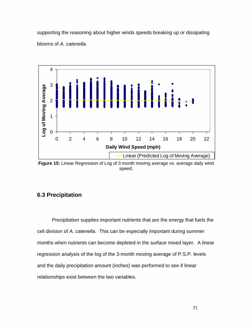
51

supporting the reasoning about higher winds speeds breaking up or dissipating

blooms of A. catenella.

0

1

2

3

4

0 2 4 6 8 10 12 14 16 18 20 22

Daily Wind Speed (mph)

Lo

g o

f M

ov

ing

Av

era

ge

Linear (Predicted Log of Moving Average)

Figure 15: Linear Regression of Log of 3 month moving average vs. average daily wind speed.

6.3 Precipitation

Precipitation supplies important nutrients that are the energy that fuels the

cell division of A. catenella. This can be especially important during summer

months when nutrients can become depleted in the surface mixed layer. A linear

regression analysis of the log of the 3-month moving average of P.S.P. levels

and the daily precipitation amount (inches) was performed to see if linear

relationships exist between the two variables.

52

The regression showed that there was a significant linear relationship

between these parameters with an F=0.0000 and p=7.64E-06, although the slope

of the line was very low, b1= -0.0622 (95% CI= -0.0895, -0.035). Indeed, a very

low R2 value of 0.0025 indicates that the variability of the log of the 3-month

moving average of P.S.P. levels is not explained by the variability of the daily

precipitation amount, and suggests that daily precipitation alone is not enough to

explain the pattern of P.S.P. levels in Washington States marine waters (Figure

16).

0

1

2

3

4

0 0.5 1 1.5 2

Daily precipitation amount (in)

Lo

g o

f M

ov

ing

Av

era

ge

Linear (Predicted Log of Moving Average)

Figure 16: Linear Regression of Log of 3 month moving average vs. daily precipitation amount (inches).

6.4 Multiple liner regression analysis

53

Though each of the above variables alone do not explain the variation in

P.S.P. levels seen in Washington States marine waters, perhaps their

combination does allow a more complex relationship to become evident. A

multiple linear regression analysis was performed using the log of the 3-month

moving average of P.S.P. levels as the response variable and a number of

explanatory variables including the ENSO index, daily ambient air temperature

(Cº), daily max wind speed (mph), average daily wind speed (mph), and daily

precipitation amount (inches).

Table 1: Multiple regression of the log of the 3 month moving average vs. the ENSO index, daily air temperature, max daily wind speed, daily wind speed, and daily

precipitation.

Adjusted R Square 0.0383

F 64.6784

Significance F 0.0000

slope

Confidence Interval Lower

95%, Upper 95% t Stat P-value

ENSO Index 0.0314 0.0236, 0.0393 7.8599 4.35E-15

Mean Daily Air Temperature (C) 0.0106 0.0092, 0.0119 15.1930 2.05E-51

Max Wind speed (mph) -0.0009 -0.0031, 0.0013 -0.7939 0.4273

Daily Wind Speed (mph) -0.0026 -0.0052, 0.0000 -1.9441 0.0519

Daily precipitation amount (in) -0.0236 -0.0516, 0.0044 -1.6509 0.0988

As we can see from the significance of F (0.0000) in Table 1 the model is

significant. Also from Table 1 we see that, despite low slope values, the first two

variables, ENSO index and Mean Daily Air Temperature, show a significant linear

relationship with P.S.P. levels. However the last three variables t-stat and p-

values indicate that these variables are not significant. The adjusted R2 indicates

54

that only 3.8% of the variability of P.S.P. levels is explained by the variability of

all these five variables, indicating the model is incomplete. However, the model

including all five explanatory variables has helped increase R2 (from <0.3% to

3.8%) compared to the simple linear models with each variable alone.

However some of the independent variables may be correlated to each

other and that may affect the outcome of the regression. A correlation analysis

shows that only two variables are correlated (Table 2), Max wind speed (mph) is

correlated with average daily wind speed (mph). This is not surprising, since a

higher average daily wind speed is likely associated with a higher max wind

speed for the same day. It also happens to be that the least significant variable

in the first multiple regression output (Table 1) is max wind speed. Thus

removing max daily wind speed from the regression may improve the model.

Table 2: Correlation output among the Independent variables.

ENSO Index

Mean Daily Air Temperature

(C)

Max Wind speed (mph)

Daily precipitation amount (in)

ENSO Index 1 Mean Daily Air Temperature (C) -0.0824 1

Max Wind speed (mph) 0.1513 -0.2053 1

Daily precipitation amount (in) 0.0234 -0.1468 0.2804 1

Daily Wind Speed (mph) 0.0577 -0.1394 0.6264 0.1709

55

The results of the updated multiple regression model (Table 3) without

max daily wind speed (mph) are described in Table 3. The significance of F

(0.0000) in table 3 indicates that this model is significant. In addition, three of the

four explanatory variables, ENSO index, daily ambient air temperature (Cº), and

average daily wind speed (mph), have a significant linear relationship with P.S.P.

levels as indicated by their t-stats and p-values. However, daily precipitation

(inches) has a low t-stat, and the p-value of 0.0627 indicates that this variable is

not significant. The adjusted R2 has not been impacted by the removal of max

wind speed from the model, indicating this second model is improved compared

to the previous model. However, only 3.8% of the variability of P.S.P. levels is

explained by these four variables, indicating the model is still poor.

Table 3: Multiple regression of the log of the 3 month moving average vs. the ENSO index, daily air temperature, daily wind speed, and daily precipitation amounts.

Adjusted R Square 0.0384

F 80.6941

Significance F 0.0000

slope

Confidence Interval Lower

95%, Upper 95% t Stat P-value

ENSO Index 0.0310 0.0232, 0.0387 7.8262 5.67E-15

Mean Daily Air Temperature (C) 0.0106 0.0093, 0.0120 15.3982 9.60E-53

Daily precipitation amount (in) -0.0260 -0.0534, 0.0014 -1.8616 0.0627

Daily Wind Speed (mph) -0.0032 -0.0053, -0.0011 -3.0441 0.0023

Daily precipitation is not significant in model 2 and a new multiple

regression (Table 4) was performed to see whether removing this variable has

56

any impact on the overall fit of the model. The results of model 3 are described in

Table 4. The significance of F (0.00) in Table 4 indicates that this model is

significant, and all the remaining variables are significant as indicated by each

variables t-stat and p-values. However, this final model with only three of the five

explanatory variables available is simpler without compromising the overall fit:

the adjusted R2 remains at the same level. Overall, given the low values of the

coefficients and the low R2, only 3.8% of the variability of P.S.P. levels is

explained by the variability of these three variables, indicating this model is also

poor. In conclusion, all these explanatory variables combined explain little of the

P.S.P. variability in Washington States marine waters and they are probably poor

predictors of high P.S.P. events.

Table 4: Multiple regression of the log of the 3 month moving average vs. the ENSO index, daily air temperature, and daily wind speed.

Adjusted R Square 0.0381

F 106.4042

Significance F 0.0000

slope Confidence Interval

Lower 95%, Upper 95% t Stat P-value

ENSO Index 0.0309 0.0232, 0.0387 7.8171 6.10E-15

Mean Daily Air Temperature (C) 0.0108 0.0095, 0.0121 15.7536 4.36E-55

Daily Wind Speed (mph) -0.0035 -0.0056, -0.0015 -3.3687 0.0008

57

Chapter 7

Implications of This Study

Before we can speculate how this study may be used we need to discuss

who may want to use it. There are four groups of individuals who would benefit

the most from this study. The first group would be the regulators and would

consist of groups or entities who are involved in the regulation of shellfish to

protect public health, such as the United States Food and Drug Administration

and the WDOH who provided the P.S.P. monitoring data as is mentioned earlier

in chapter 5. These are only a few local examples of what a regulator is;

however there are many different types of regulatory agencies worldwide who

would benefit from this information and who may be able to apply a similar study

to other toxic algal species.

The second group would consist of those who harvest shellfish to sell.

This would include shellfish harvesters, growers, and distributors (not equal to

processors). Washington’s shellfish industry is multi-billion dollar industry, and is

economically a very important part of Washington State’s economy. Washington

is the leading producer of farmed bivalve shellfish in the United States,

generating an estimated $77 million in sales (Figure 17) and accounting for 86

percent of the West Coast's production in the year 2000 (http://www

.psat.wa.gov/Programs/shellfish/fact_sheets/economy_web1.pdf). The cost of

58

P.S.P. to the commercial fishery, recreational harvesters, and the aquaculture

industry is believed to exceed $10 million annually (http://www.

nwfsc.noaa.gov/hab/outreach /pdffiles /RedTides2000.pdf).

The third group would be comprised of consumers and individuals who

harvest shellfish for recreation, as well as Native American tribes in Washington

State who harvest shellfish for subsistence, ceremonial harvesting, or for market.

The fourth group would be fellow scientists who may find this study useful in their

own endeavors to better understand why toxic species of phytoplankton exhibit

such variability in between years as well as within year.

Figure 17: Estimated West Coast production of farmed oysters, clams, mussels and

geoduck, 2000 http://www.psat.wa.gov/Programs/shellfish/fact_sheets/economy_ web1.pdf.

The remainder of this chapter is divided into three sections to discuss the

implications this study may have for those that are impacted by P.S.P. in

Washington’s marine waters. The first section will cover the regulatory

implications this study may have. The second section will look at the benefits

59

this study may have for shellfish harvesters, growers, and distributors, whom for

the purpose of this study will be called the shellfish industry, this includes tribal

harvest for commercial sale. The third section will cover how this information

may be important to consumers of shellfish including recreational harvesters, and

the Native American tribes around Puget Sound and on Washington States

Coastal areas.

7.1 Regulatory Agencies and/or Groups

“The Washington State Department of Health (WDOH) monitors biotoxin

levels in shellfish from sites throughout Western Washington to protect

consumers from poisoning by naturally occurring biotoxin’s that if present can

accumulate in shellfish tissue” (Determan, 2003). Better understanding how and

why levels of P.S.P. in Washington State’s marine waters fluctuate the way they

do would be a great advantage in trying to predict when a bloom of P.S.P. may

occur and prevent illness outbreaks before they happen.

The WDOH has been very successful to date with their P.S.P. monitoring

program in preventing illness. However, sometimes there are questions about

how to treat rising levels of P.S.P. that have not gone above the 80µg STX/100g

of shellfish tissue needed to close a beach. When shellfish areas are open for

harvesting the WDOH samples biweekly unless a sample has detectable levels

of P.S.P. which is equal to or greater than 38µg STX/100g, at which time they

60

start sampling weekly. Samples are also submitted for testing prior to any tribal

harvest for commercial, ceremonial and subsistence harvesting (Cox, 2001).

One final recommendation would be to collect more local environmental

data such as water temperature, salinity, air temperature, wind speed and

direction, and rain data and look for relationships that may help to predict blooms

of P.S.P. A complete data set of environmental parameters taken in conjunction

with P.S.P. samples would greatly facilitate the effort to find the most reliable

environmental indicator and predictors of rising P.S.P. levels.

7.2 Shellfish Industry

The Shellfish industry primarily grows, harvests, and distributes the many

diverse and abundant species of commercial shellfish in Washington State.

However, many of the industry are involved in one way or another with the

regulatory aspects and decision making processes of the government. The

shellfish industry is also involved in projects to enhance shellfish beds through

environmental enhancement of the surrounding areas. Since there are many

species of shellfish harvested for commercial purposes in Washington State and

just as many ways to harvest them, this study may need to be applied on a case

by case basis as needed. However, this study may prove useful to the shellfish

industry in a variety of ways such as the ones listed below.

If a relationship can be found between the phases of ENSO and local

P.S.P. levels, then the shellfish industry may want to plan to stop or reduce their

61

harvesting of shellfish during times and phases of ENSO that may be more likely

to have higher levels of P.S.P. present. In order to limit the amount of product

recalled or destroyed, because it gets harvested but does not get sold. This may

be especially beneficial to those companies that harvest species of commercial

shellfish that retain P.S.P. longer in their systems then other shellfish thus

prolonging the unsafe harvest period. For example “Blue mussels (Mytilus

edulis) are quick to pick up P.S.P. toxin and also quick to purge the toxin, once

the mussels stop feeding on the toxic algae. At the other extreme are shellfish

such as Butter clams (Saxidomus nuttalli), that are slow to pick up P.S.P. toxin

and are also slow to purge the toxin” (Cox, 2001).

The shellfish Industry may want to plan for periods when ENSO has the

possibility to impact their business negatively such as mentioned above. They

can potentially avoid the costs of P.S.P. related closures to their businesses by

choosing to not harvest or test more rigorously/frequently during times when

P.S.P. may have the potential to be higher, thus ensuring that the product will not

get recalled and result in immediate loss of money as well as keeping the

shellfish for future sales.

An outbreak of P.S.P. during November and December in 1997 (this

apparently is not the rule: it just happened to be an El Nino phase: it doesn’t

mean that the same should be expected in future El Nino phases, there is not a

good correlation or relationship between the two, and therefore it has no

predictive value) is a good example of the economic hardships P.S.P. has had on

the Shellfish industry that can potentially be mitigated, if a relationship between

62

ENSO and P.S.P. levels exist and can be used to predict when levels of P.S.P.

will be higher. The 1997 P.S.P. blooms severely impacted the oyster harvest in

Puget Sound and in the coastal estuaries of Willapa Bay and Grays Harbor.

Many of the small farms in these areas were closed and suffered great financial

losses.

“A Puget Sound-area farmer of clams and oysters said that he was forced to

close for eight weeks, causing him to miss out on Thanksgiving, Christmas, and

New Year’s sales, and estimated his losses to be $5,000 per week. The P.S.P.

bloom in Willapa Bay and Grays Harbor was felt just before Thanksgiving Day,

which in the oyster industries is the busiest time of the year, accounting for 40%

of the year’s business. Although the coastal bays were reopened by mid-

December, sales during the Christmas season were also lost because out-of-

state competitors had moved into the market. About 34 coastal shellfish farms

lost approximately 50% of their sales, reducing average sales by about $8

million. Over 100 workers were laid off and many more had hours reduced”

(http://www.nwfsc.noaa.gov/hab/outreach/pdffiles/RedTides 2000.pdf). Not only

did the small oyster farms suffer in 1997, the entire shellfish industry felt the

economic impacts of the P.S.P. bloom. Large companies had to scale back

shellfish farming in the coastal estuaries as well as in Puget Sound resulting in

the loss of, oyster diggers and shuckers, jobs throughout the state.

One of the processes of shellfish enhancement is to seed the actual

shellfish beds with oysters, clams, and geoduck seeds or inoculums. Different

environmental parameters work better for seeding shellfish beds. Though it is

63

beyond the scope of this paper, enhancing shellfish beds during one phase of

ENSO may prove to have more productive results then the other phases.

7.3 Recreational Harvest and Tribal Ceremonial/Subsistence

Harvesting

Thousands of recreational shellfish harvesters participate in the extremely

popular razor clam fishery in Washington State each year. When recreational

shellfish harvest is closed due to the presence of toxic algae, recreational

harvesters are deprived from their favorite activity and food, but it is not only

them that bear the impact. Recreational shellfish harvesting provides a

significant economic support to local coastal communities especially for service

businesses. Therefore, it is also the hundreds of business owners, and the

thousands employed by them, who greatly suffer from the loss of money spent by

clam diggers that stay overnight or pass through Washington’s many small

coastal communities. The annual value of the coastal razor clam fishery is

estimated at $12 million recreationally and another $7 million commercially

(http:// www.psat.wa.gov/ Programs/shellfish/factsheets/economyweb1.pdf).

Washington’s Puget Sound basin and coastal regions are a unique area

where treaty Indian tribes reside. For ceremonies, subsistence, and commercial

sales, these tribes depend on the harvest of marine species such as oysters,

razor clams, California mussels, littleneck clams, horse clams, butter clams,

gooseneck barnacles and Dungeness crabs. Unfortunately, all of these species

64

can accumulate toxins by filtering seawater. When toxins reach levels too

dangerous for human consumption, tribes can face tremendous economic and

quality-of-life losses. Because of declining fish stocks in the Pacific Northwest,

including rockfish and salmon, tribes are relying more heavily on shellfish then

ever before. Shellfish and crustaceans are a primary source of income to many

tribal members.

The commercial harvest of shellfish by Washington’s Indian tribes would

benefit from this study in the same way as indicated above for the rest of the

shellfish industry. The current WDOH monitoring program will ensure the

continued safety and health of the tribe’s subsistence and ceremonial harvests

by continuing to have samples submitted and tested prior to their consumption or

use. However if one phase of ENSO tends to have higher average P.S.P. levels,

perhaps the tribes may want to be prepared to offset the harvest of shellfish with

alternative food sources and income, though this may not be a viable solution for

all tribes. It is beyond the scope of this paper to provide alternatives, but this is

an important subject to look into in the future so that the Tribes can continue to

sustain their way of life and cultural integrity during those times when P.S.P.

makes the harvest of shellfish unsafe.

65

Chapter 8

Conclusion

Knowing how A. catenella and other harmful algal booms are affected by

the physical processes of their environment may lead us to an answer about why

they are becoming more widespread globally. It may also provide some insight

into why we are seeing the annual patterns of harmful algal blooms, in

Washington State’s marine waters and other coastal areas, that we are and why

they are becoming more widespread globally. From a policy and health

perspective understanding how and why A. catenella is affected by its

environment, and the physical processes associated with it, may lead policy

makers and local health officials to a better understanding of how to predict and

monitor outbreaks of harmful algal species such as A. catenella.

Understanding why P.S.P. levels in Washington State’s marine waters

have such variability inter-annually and seasonally will help in mitigating the

impacts to Washington’s economy and health. This understanding will also

enable regulatory officials to predict when levels of P.S.P. are more likely going

to be higher then average. This will also help shellfish growers and harvesters to

attempt to mitigate the impacts of P.S.P. to their businesses and in turn

Washington’s economy and health as stated in chapter 7. However,

understanding how the physical properties of A. catenellas environment

influences its production of P.S.P. is still something that needs to be determined

66

more accurately. One direction to take would be to attempt to understand how

levels of P.S.P. in Washington change with regional and global weather patterns

such as ENSO.

Even though no relationship was found between ENSO and P.S.P. levels

in this study it does not mean that one does not exist. It may be a more complex

relationship involving other phenomena and combined with variations in local

parameters. The limitations of the data availability at this time limit this study’s

ability to determine what is the relationship between large scale climate

phenomena’s such as ENSO and localized P.S.P. levels, if one does exist.

Given that the global scale ENSO index is not adequate by itself in explaining

variations of P.S.P. levels, and neither ENSO nor three local weather parameters

combined explain more then 3.8% of P.S.P. variability, more detailed information

about local parameters is needed. It would be important to continue to monitor A.

catenellas response to localized weather patterns and relate these to large scale

climate indicators such as ENSO for future studies.

Due to the long-term variability (centennial) of the phases of ENSO, this

study will be more complete as more data are gathered, thus as time goes on we

will have a longer timescale beyond just a few decades to compare P.S.P. levels

to the phases of ENSO. At the same time the monitoring program at the WDOH,

will hopefully continue to collect more P.S.P. samples and add a environmental

data collection aspect to their monitoring program, though more funding may be

required for this. This will also help to ensure a more robust analysis in the

future. If more toxic algae monitoring programs continue to gather and maintain

67

long term databases, in other states and countries, then perhaps others groups

will find that the phases of ENSO, or similar large scale climate phenomena’s, do

have an influence on the levels of toxins present in their areas. The more we

know about toxic species of algae as a whole the more we can begin to

understand the patterns of toxicity (present in space and time) associated with

them.

Determining how regional climate and weather affect P.S.P. levels will not

help us to completely stop the impact of P.S.P. to Washington’s economy and

health; however, if used properly they should help to reduce the impact. And if

more local environmental data are collected in conjunction with P.S.P.

samples over time, perhaps we will be able to determine a relationship

between a physical property of A. catenellas environment and its P.S.P.

production. If a relationship can be determined then we can try to correlate the

physical property responsible with the different phases of ENSO in an attempt to

become more precise in predicting P.S.P. outbreaks. The more we understand

the better we can mitigate the impacts of P.S.P.

68

References:

1. Anderson M. Donald. 1998. Physiological Ecology of Harmful Algal

Blooms: Physiology and Bloom Dynamics of Toxic Alexandrium Species, with Emphasis on Life Cycle Transitions. Ecological Sciences, vol. 41: pg 29-48

2. Anderson M. Donald. 2004. The Growing Problem of Harmful Algae.

Oceanus, vol. 43, No. 1: pg. 34-39 3. Anderson M. Donald, Pitcher C. Grant, Estrada Marta. 2005. The

comparative “Systems” Approach to HAB Research. Oceanography, vol. 18, No. 2: pg. 148-157

4. Anonymous. 2005. North American Countries Reach Consensus on El

Niño, La Niña Definitions. Bulletin of the American Meteorological Society, vol. 86, Iss. 4: pg. 473-474

5. Climate Impacts Group. 2008. Impacts of Natural Climate Variability on

Pacific Northwest Climate. University of Washington, Seattle, WA. http://cses.washington.edu/cig/pnwc/ci/shtml

6. Frank Cox. 2001. Washington’s Marine Biotoxin Monitoring Program.

Washington State Department of Health, Olympia, WA. 7. Determan Tim. 2003. Paralytic Shellfish Poisoning (P.S.P.) Patterns in

Puget Sound Shellfish in 2001. Washington State Department of Health, vol. 1: pg. 1-14

8. Donaghay L. Percy, Osborn R. Thomas. 1997. Towards a Theory of

Biological-Physical Control of Harmful Algal Bloom Dynamics and Impacts. Limnology and Oceanography, vol. 42, No. 5, part 2: pg. 1283-1296

9. Enloe Jesse, O’Brien James, Smith R. Shawn. 2004. Notes and

Correspondence: ENSO Impacts on Peak Wind Gusts in the United States. American Meteorological society, vol. 17: pg. 1728-1737

10. Estrada Marta, Berdalet Elisa. 1998. Physiological Ecology of Harmful

Algal Blooms: Effects of Turbulence on Phytoplankton. Ecological Sciences, vol. 41: pg 601-618

11. Fourth Assessment Report of the IPCC. 2007. Observation: Surface and

Atmospheric Climate Change. IPCC, vol. 4 chapter # 3: pg. 287-292

69

12. Gentian Patrick, Donaghay Percy, Yamazaki, Raine Robin, Reguera Beatriz, Osborn Thomas. 2005. Harmful Algal Blooms in Stratified Environments. Oceanography, vol. 18, No. 2: pg. 172-183

13. Gershunov Alexander, Barnett P. Tim. 1998. ENSO influence on

Intraseasonal Extreme Rainfall and Temperature Frequencies in the Contiguous United States: Observations and Model Results. American Meteorological society, vol. 11: pg. 1575-1586

14. Glantz M., Katz R., Nicholls N. 1991. Teleconnections Linking Worldwide

Climate Anomalies. Cambridge University Press, Cambridge. 15. Glibert M Patricia, Seitzinger Sybil, Heil A. Cynthia, Burkholder M. Joann,

Parrow W. Mattew, Codispoti A. Louis, Kelly Vince. 2005. The Role of Eutrophication in the Global Proliferation of Harmful Algal Blooms New Perspectives and New Approaches. Oceanography, vol. 18, No. 2: pg. 198-209

16. Halstead B.W. 1965. Poisonous and Venomous Marine Animals of the

World, Volume 1, Invertebrates. U.S. Government Printing Office, D.C. Washington: pg. 25

17. Hamlet F. Alan. 1997. Climate Change in the Columbia River Basin.

JISAO Climate Impacts Group-University of Washington, pg.1-6 18. Hanley E. Deborah, Bourassa A. Mark, O’Brien J. James, Smith R.

Shawn, Spade R. Elizabeth. 2003. Notes and Correspondence: quantitative Evaluation of ENSO Indices. American Meteorological society, vol. 16: pg. 1249-1258

19. Katz W. Richard. 2002. Sir Gilbert Walker and a Connection between El

Niño and Statistics. Statistical Science, vol. 17, No. 1: pg. 97-112 20. Navarroa J. M., Munoz M.G., Contreras A.M. 2006. Temperature as a

factor regulating growth and toxin content in the dinoflagellate Alexandrium catanella. Harmful Algae, vol. 5: pg. 762-769

21. Ropelewski C.F., Halpert M.S. 1986. North American Precipitation and

Temperature Patterns Associated with the El Niño/Southern Oscillation (ENSO). Monthly Weather Review, vol. 114: pg. 2352-2362

22. Sharples Jonathan, Moore C. Mark, Rippeth P. Tom, Holligan M. Patrick,

Hydes J. David, Fisher R. Neil, Simpson H. John. 2001. Phytoplankton Distribution and Survival in the Thermocline. Limnology and Oceanography, vol. 46 No. 3: pg. 486-496

70

23. Smayda J. Theodore. 1997. Harmful algal Blooms: Their Ecophysiology and General Relevance to Phytoplankton Blooms in the Sea. Limnology and Oceanography, vol. 42, No. 5, Part 2:pg. 1137-1153

24. Stewart T. Iris, Cayan R. Daniel, Dettinger D. Michael. 2005. Changes

toward Earlier Streamflow Timing across Western North America. Journal of Climate, vol. 18: pg. 1136-1155

25. Sullivan M. James, Swift Elijah, Donaghay L. Percy, Rines E.B. Jan. 2003.

Small-scale turbulence affects the division rate and morphology of two red-tide dinoflagellates. Harmful Algae, vol. 2: pg. 183-199

26. Trainer L. Vera, Eberhart L. Bish-Thuy, Wekell C. John, Adams G.

Nicholaus, Hanson Linda, Cox Frank, Dowell Judy. 2003. Paralytic-Shellfish Toxins in Puget Sound, Washington State. Journal of Shellfish Research, vol. 22, No. 1: pg. 213-223

27. Webster J. Peter, Palmer N. Timothy. 1997. The Past and the Future of El

Niño. Nature, vol. 390: pg. 562-564 28. Weise M. Andrea, Levasseur Maruice, Sucier J. Fancois, Senneville

Simon. 2002. The link between precipitation, river runoff, and blooms of the toxic dinoflagellate Alexandrium tamarense in the St. Lawrence. Canadian Journal of Fisheries and Aquatic Sciences, Vol. 59, No. 3: pg. 464-474

29. UW Climate Impacts Group (CIG). 2004. Overview of Climate Change

Impacts in the U.S. Pacific Northwest. University of Washington Climate Impacts Group, vol. 1:pg. 1-13

30. yamamoto Tamiji, Hahimoto Toshiya, Tarutani Kenji, Kotani Yuichi. 2002.

Effects of winds, tides, and river water runoff on the formation and disappearance of the alexandrium tamarense bloom in Hiroshima Bay, Japan. Harmful Algae, vol. 2: pg. 301-312