The Region Smoothing Swap Game

Allison Henrich, Inga Johnson, Jonah Ostroff

September 30, 2019

Abstract

We introduce a topological combinatorial game called the RegionSmoothing Swap Game. The game is played on a game board de-rived from the connected shadow of a link diagram on a (possiblynon-orientable) surface by smoothing at crossings. Moves in the gameare performed on regions of the diagram and can switch the direc-tion of certain crossings’ smoothings. The players’ goals relate to theconnectedness of the diagram produced by game play.

1 Introduction.

We introduce a new game, the Region Smoothing Swap Game,played on a game board derived from the connected shadow of a linkdiagram on a surface by smoothing at the diagram’s crossings. Thisgame can be viewed as a hybrid of the Link Smoothing Game, studiedin [2], and the Region Unknotting Game, studied in [1].

Suppose that D is a connected diagram of a link shadow on some(possibly non-orientable) surface S. That is, D is a connected link di-agram where under- and over-strand information is unspecified at thecrossings. The unspecified crossings are called precrossings. Thereare two possible options for smoothing each precrossing, shown in Fig-ure 1. When every precrossing of a link diagram D has been smoothed,the result is called a smoothed state or a smoothing of D. A regionsmoothing swap is an operation that replaces one smoothed state bythe state corresponding to changing the smoothings of all crossingson the boundary of a particular region in the link diagram. Figure 2shows a link together with two of its connected smoothed states. (Thelocations of the smoothed precrossings are indicated in the diagram bygrey disks.) These two states are related by a single region smoothingswap, performed on the highlighted region.

Game play begins on a connected smoothed state of link diagramD on a surface S. Two players take turns making moves. During

1

arX

iv:1

909.

1237

0v1

[m

ath.

CO

] 2

6 Se

p 20

19

Figure 1 – Smoothing a precrossing.

Figure 2 – The shadow of a twist knot and two connectedsmoothed states of the diagram. Unless otherwise specified,we assume that our diagrams lie on a sphere.

game play, the smoothed diagram may become disconnected. A moveconsists of choosing a region in the link diagram and either performinga region smoothing swap at that region or keeping the state as-is. Thetwo players continue selecting regions and moving until all regions of Don S have been selected exactly once. One player plays with the goal ofproducing a connected smoothed state when game play ends while theother player wants the game to end with a disconnected diagram. Wewill call the player that wants to keep the diagram connected PlayerC and the player whose goal is to disconnect the diagram Player D.

An example game is played in Figure 3. As each region is selected,the blue shading indicates that there is no change to the smoothingsalong the boundary of the region; the green shading indicates the ad-jacent smoothings are switched.

In this paper, our goal is to classify connected smoothed statesof link shadows on various surfaces according to which player has awinning strategy in the Region Smoothing Swap Game. In general,Player D typically has a strong advantage in this game. This is becausean arbitrary choice of smoothings for the crossings in a link diagramis far more likely to result in a state that has two or more connectedcomponents than in a state with a single component. Indeed, somelinks have equivalence classes of smoothed states (where equivalenceis generated by the smoothing swap operation) that don’t contain anyconnected states. So, we aim to identify link shadows with smoothedstates on which Player C has a winning strategy. We always begin with

2

BeginMove 4,

D

Move 1, CMove 5,

C

Move 2, DMove 6,

D

Move 3, CMove 7,

C

Figure 3 – The Region Smoothing Swap Game is played ona 5-crossing knot shadow that lies on a sphere. C plays firstand wins.

a game board that is connected to ensure that we are in an equivalenceclass that contains at least one connected state.

The example in Figure 3 shows game play on a link diagram anda particular smoothed state where C moves first and C wins. In fact,on this particular game board, C can always win if she moves first. Tounderstand why Player C has a winning strategy, we first translate thegame into a game on graphs to simplify our analysis.

2 Graphs and the Region Smoothing SwapGame.

It can be useful to shift from viewing our game on a link diagram toviewing it as a game on the corresponding checkerboard graph. In thisnew setting, the regions of the smoothed link diagram are representedby either a vertex or a face of the graph. The smoothed crossings arerepresented by the edges of the graph. We see that the connectednessof a subset of edges in the graph captures the connectedness of thecorresponding link diagram.

Let’s recall how to form the checkerboard graph corresponding toa link shadow. We start by checkerboard coloring the shadow, thenplacing a vertex in each shaded region. Whenever two shaded regionsare connected by a precrossing, we connect the associated vertices with

3

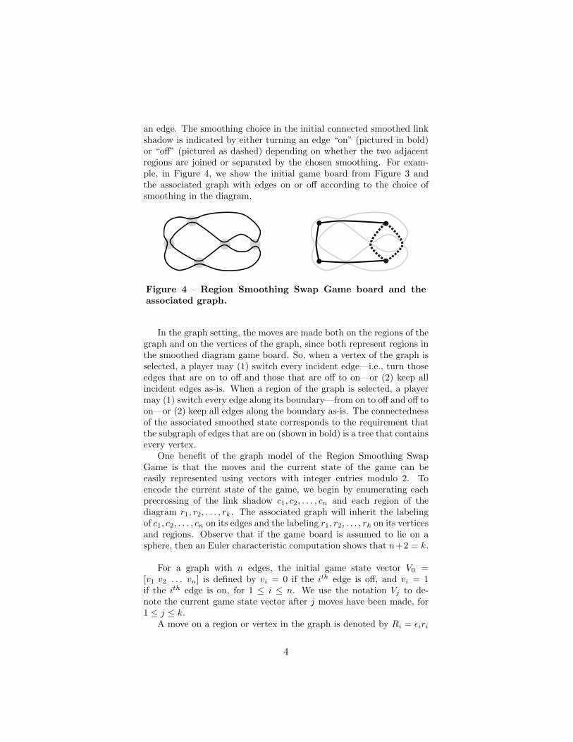
an edge. The smoothing choice in the initial connected smoothed linkshadow is indicated by either turning an edge “on” (pictured in bold)or “off” (pictured as dashed) depending on whether the two adjacentregions are joined or separated by the chosen smoothing. For exam-ple, in Figure 4, we show the initial game board from Figure 3 andthe associated graph with edges on or off according to the choice ofsmoothing in the diagram.

Figure 4 – Region Smoothing Swap Game board and theassociated graph.

In the graph setting, the moves are made both on the regions of thegraph and on the vertices of the graph, since both represent regions inthe smoothed diagram game board. So, when a vertex of the graph isselected, a player may (1) switch every incident edge—i.e., turn thoseedges that are on to off and those that are off to on—or (2) keep allincident edges as-is. When a region of the graph is selected, a playermay (1) switch every edge along its boundary—from on to off and off toon—or (2) keep all edges along the boundary as-is. The connectednessof the associated smoothed state corresponds to the requirement thatthe subgraph of edges that are on (shown in bold) is a tree that containsevery vertex.

One benefit of the graph model of the Region Smoothing SwapGame is that the moves and the current state of the game can beeasily represented using vectors with integer entries modulo 2. Toencode the current state of the game, we begin by enumerating eachprecrossing of the link shadow c1, c2, . . . , cn and each region of thediagram r1, r2, . . . , rk. The associated graph will inherit the labelingof c1, c2, . . . , cn on its edges and the labeling r1, r2, . . . , rk on its verticesand regions. Observe that if the game board is assumed to lie on asphere, then an Euler characteristic computation shows that n+2 = k.

For a graph with n edges, the initial game state vector V0 =[v1 v2 . . . vn] is defined by vi = 0 if the ith edge is off, and vi = 1if the ith edge is on, for 1 ≤ i ≤ n. We use the notation Vj to de-note the current game state vector after j moves have been made, for1 ≤ j ≤ k.

A move on a region or vertex in the graph is denoted by Ri = εiri

4

where ri = [mi,1 mi,2 . . . mi,n] is defined by mi,j = 1 if the edge cjis in the boundary of region ri or incident to vertex ri, and mi,j = 0otherwise. The value of εi is 1 or 0 depending on whether the playerwants to switch all edge values or keep them as is. The effect of themove Ri on game state vector Vj is Vj+1 = Vj +Ri modulo 2.

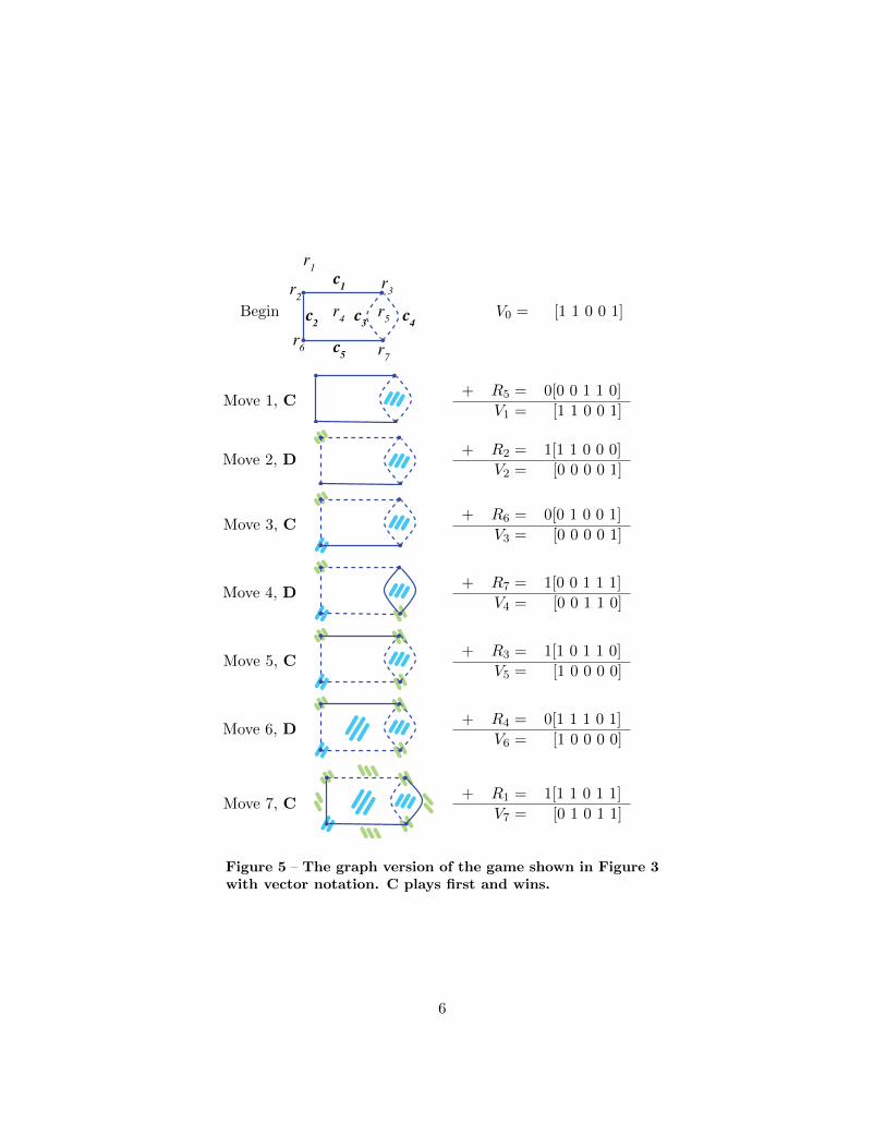
As an example, the game play from Figure 3 is represented withvectors in Figure 5.

By the commutativity of vector addition, the example in Figure 5shows that the entire game play can be captured by the followingmatrix equation.

V7 = V0 +R1 +R2 + · · ·+R7

= V0 + ε1r1 + ε2r2 + · · ·+ ε7r7

= V0 + [ε1 ε2 . . . ε7]

r1r2...r7

In general, given a connected state vector V0, our goal is to strate-

gically pick, or as we shall see pair, the values εi for 1 ≤ i ≤ k so thatthe resulting state vector Vk from Equation 1 represents a connecteddiagram.

Vk = V0 + [ε1 ε2 . . . εk]

r1r2...rk

(1)

Using this formalism, we can determine a general winning strategyfor Player C for the example in Figure 5. Player C moves on r5 first,keeping the region as-is. The remaining moves are determined by pair-ing moves on the following regions/vertices: r1 and r4, r2 and r6, andr3 and r7. In each pair, for any move made by D, there is a corre-sponding response move by C. In particular, Player C should respondto D’s moves by choosing ε1 6= ε4, ε2 6= ε6, and ε3 = ε7. Regardless ofwhich vertices/regions Player D decides to move on and which signsfor εi he chooses, C’s response guarantees a connected diagram willresult. Why is this? Consider the following matrix representing ourgame board.

5

Begin

c1

c5

c4

c3

c2

r4

r3r

2

r1

r5

r6 r

7

V0 = [1 1 0 0 1]

Move 1, C+ R5 = 0[0 0 1 1 0]

V1 = [1 1 0 0 1]

Move 2, D+ R2 = 1[1 1 0 0 0]

V2 = [0 0 0 0 1]

Move 3, C+ R6 = 0[0 1 0 0 1]

V3 = [0 0 0 0 1]

Move 4, D+ R7 = 1[0 0 1 1 1]

V4 = [0 0 1 1 0]

Move 5, C+ R3 = 1[1 0 1 1 0]

V5 = [1 0 0 0 0]

Move 6, D+ R4 = 0[1 1 1 0 1]

V6 = [1 0 0 0 0]

Move 7, C+ R1 = 1[1 1 0 1 1]

V7 = [0 1 0 1 1]

Figure 5 – The graph version of the game shown in Figure 3with vector notation. C plays first and wins.

6

R =

r1r2r3r4r5r6r7

=

1 1 0 1 11 1 0 0 01 0 1 1 01 1 1 0 10 0 1 1 00 1 0 0 10 0 1 1 1

(2)

If Player C follows the strategy outlined above, the following arethe eight possibilities for the vector E = [ε1 ε2 . . . ε7]. The vectorsrepresent the game play choices for Player D, with Player C’s strategyentirely determined by D’s choices. Note that the first vector in thelist represents the game play shown in Figure 5.

[1 1 1 0 0 0 1

][1 1 0 0 0 0 0

][1 0 1 0 0 1 1

][1 0 0 0 0 1 0

][0 1 1 1 0 0 1

][0 1 0 1 0 0 0

][0 0 1 1 0 1 1

][0 0 0 1 0 1 0

]Multiplying each of these E vectors by the R matrix in Equation

2 and adding the vector V0 = [1 1 0 0 1] gives the following eightvectors, the resulting values for V7 that represent the states of the finalgame board.

[0 1 0 1 1

][1 1 0 1 0

][1 1 0 1 0

][0 1 0 1 1

][0 1 1 0 1

][1 1 1 0 0

][1 1 1 0 0

][0 1 1 0 1

]7

As we can see, there are only four distinct ending game states thatare possible if D has freedom to choose his own moves and C follows herstrategy. The corresponding graphs are shown in Figure 6. Note thatthe subgraphs defined by the edges that are turned on are all spanningtrees in the checkerboard graph. Thus, the strategy we described isindeed a winning strategy.

[0 1 0 1 1] [1 1 0 1 0]

[0 1 1 0 1] [1 1 1 0 0]

Figure 6 – The possible ending game boards when C followsher winning strategy on the graph in Figure 4.

(a) (b) (c)

Figure 7 – All connected starting game boards on a 5-crossingtwist knot shadow, grouped according to winning strategy.

As we can see in Figure 2, there are many possible starting gameboards that come from the twist knot. In Figure 7 we list all possi-ble starting game graphs and group them according to their winningpairing strategy for C. We will see that the pairs of moves describedabove remain quite useful on any starting game board. In fact, themove pairing strategy can be used to prove the following theorem.

Proposition 1. If Player C moves first, then Player C has a winningstrategy playing the Region Smoothing Swap Game on any connectedgame board associated to the 5-crossing twist knot shadow in Figure 2.

Proof. All connected starting game boards are shown in Figure 7 andplaced in one of three groups labeled (a), (b), and (c). For each group ofstarting game boards, we describe a winning strategy for C, assuming

8

she moves first. We use the names of regions, ri, and crossings, cj , asgiven in Figure 5. In all groups, Player C’s first move is on r5 and shekeeps the region as-is.

For any starting board in group (a), we observe the following pairingstrategy results in a win for C: ε1 = ε4, ε2 = ε6, and ε3 = ε7. Infact, after any single pair of moves ε1 = ε4, ε2 = ε6, or ε3 = ε7, themimicking strategy results in another game board within the list ofFigure 7(a). Thus, player C can defend the boards in group (a) so thatafter each move by D and corresponding reply by C, the board returnsto a connected game board from group (a).

For any starting board in group (b), we observe the following pair-ing strategy results in a win for C: ε1 = ε4, ε2 6= ε6, and ε3 = ε7. Recallthat, for any given set of moves, the order in which they are performeddoesn’t affect the outcome of the game. So, without loss of generality,we suppose the pair of moves ε2 6= ε6 are made first. After these twomoves are made on a game board from (b), the result is a game boardfrom (a). Then the remaining pairs of moves ε1 = ε4 and ε3 = ε7 areapplied to a game board from group (a), resulting in final board ingroup (a).

Lastly, as we saw in the more detailed linear algebraic argumentabove for the game board (c), the following pairing strategy results in awin for C: ε1 6= ε4, ε2 6= ε6, and ε3 = ε7. This pairing works regardlessof the order in which the paired moves are applied. When playing onthe board in group (c), we note that if both pairs of moves ε1 6= ε4and ε2 6= ε6 are completed first, then the result is a connected gameboard from (a). The final pair of moves, ε3 = ε7, completes the game,producing a game board from (a).

We observe the special role played by the game boards in group (a)of Figure 7. Once the starting board graph was moved into a board oftype (a) by Player C, then C had a winning defensive strategy.

3 Game Play on the Sphere

Three nice examples of link shadows on the surface of a sphere on whichPlayer C has a winning strategy come from the minimum crossingdiagrams of the figure-eight knot, the trefoil, and the Borromean rings.The figure-eight knot in particular gives a nice example of a game thatPlayer C can win using a mimicking strategy.

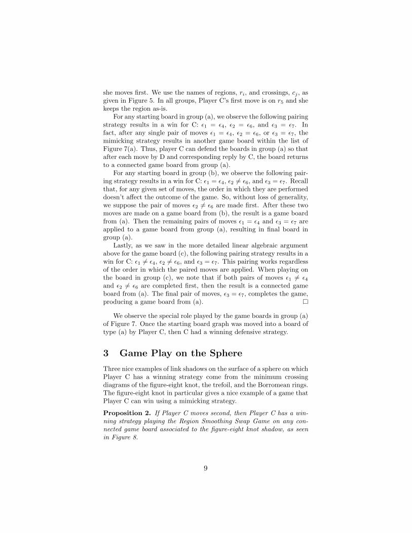
Proposition 2. If Player C moves second, then Player C has a win-ning strategy playing the Region Smoothing Swap Game on any con-nected game board associated to the figure-eight knot shadow, as seenin Figure 8.

9

r1

r2

r3

c1

c3

c2

r6

r4

r5

c4

Figure 8 – The figure-eight knot and a corresponding gameboard.

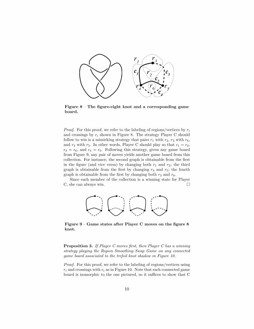
Proof. For this proof, we refer to the labeling of regions/vertices by riand crossings by ci shown in Figure 8. The strategy Player C shouldfollow to win is a mimicking strategy that pairs r1 with r2, r3 with r6,and r4 with r5. In other words, Player C should play so that ε1 = ε2,ε3 = ε6, and ε4 = ε5. Following this strategy, given any game boardfrom Figure 9, any pair of moves yields another game board from thiscollection. For instance, the second graph is obtainable from the firstin the figure (and vice versa) by changing both r1 and r2; the thirdgraph is obtainable from the first by changing r4 and r5; the fourthgraph is obtainable from the first by changing both r3 and r6.

Since each member of the collection is a winning state for PlayerC, she can always win.

Figure 9 – Game states after Player C moves on the figure 8knot.

Proposition 3. If Player C moves first, then Player C has a winningstrategy playing the Region Smoothing Swap Game on any connectedgame board associated to the trefoil knot shadow in Figure 10.

Proof. For this proof, we refer to the labeling of regions/vertices usingri and crossings with ci as in Figure 10. Note that each connected gameboard is isomorphic to the one pictured, so it suffices to show that C

10

r1

r2

r3

r5

c3

c2

c1

r4

Figure 10 – The trefoil and a corresponding game board.

has a winning strategy on this particular board. Let Player C movefirst on r5, the region that contains the vertex of degree 2, keeping itas-is. For the remaining moves, we pair r1 with r2 and r3 with r4, andensure that C follows a strategy such that ε1 = ε2 while ε3 6= ε4. So,for instance, if D moves on r1 and performs a smoothing swap, thenC performs a smoothing swap on r2. Any moves on r1 and r2 thatsatisfy ε1 = ε2 produce a graph that is identical to the starting graph.If, on the other hand, D moves on r3 and leaves it as-is, then C shouldperform a smoothing swap on r4. The resulting graph is isomorphicto the original graph. Any other pair of choices following the ε3 6= ε4strategy similarly produces an isomorphic graph.

Proposition 4. Suppose the Region Smoothing Swap Game is playedon a connected starting board determined by the Borromean rings (pic-tured in Figure 11). Then Player C has a winning strategy when play-ing second.

Figure 11 – The Borromean rings and a corresponding gameboard.

Proof. We begin with the standard representation of the Borromeanrings and the connected game board shown in Figure 11. Notice thatthe associated graph—which we see is the complete graph on four

11

(a) (b)

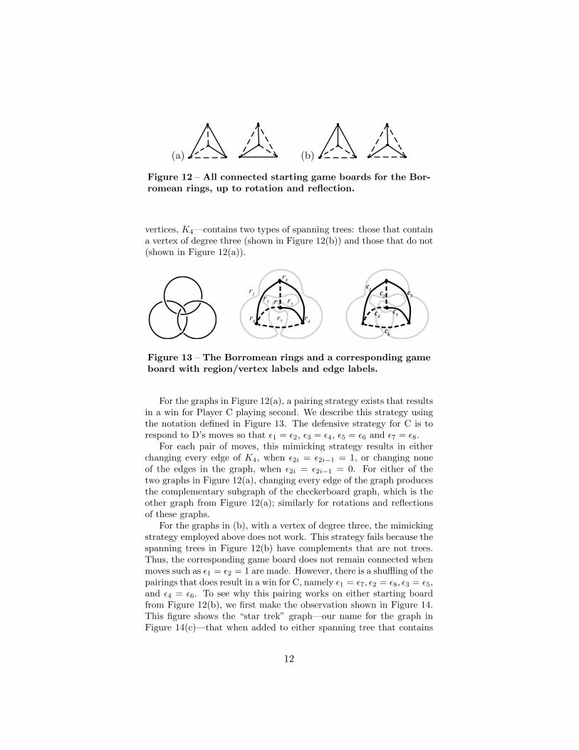
Figure 12 – All connected starting game boards for the Bor-romean rings, up to rotation and reflection.

vertices, K4—contains two types of spanning trees: those that containa vertex of degree three (shown in Figure 12(b)) and those that do not(shown in Figure 12(a)).

r1

r4

r5

r6

r8

r7

r3 r

2

c1c2

c5

c6

c4

c3

Figure 13 – The Borromean rings and a corresponding gameboard with region/vertex labels and edge labels.

For the graphs in Figure 12(a), a pairing strategy exists that resultsin a win for Player C playing second. We describe this strategy usingthe notation defined in Figure 13. The defensive strategy for C is torespond to D’s moves so that ε1 = ε2, ε3 = ε4, ε5 = ε6 and ε7 = ε8.

For each pair of moves, this mimicking strategy results in eitherchanging every edge of K4, when ε2i = ε2i−1 = 1, or changing noneof the edges in the graph, when ε2i = ε2i−1 = 0. For either of thetwo graphs in Figure 12(a), changing every edge of the graph producesthe complementary subgraph of the checkerboard graph, which is theother graph from Figure 12(a); similarly for rotations and reflectionsof these graphs.

For the graphs in (b), with a vertex of degree three, the mimickingstrategy employed above does not work. This strategy fails because thespanning trees in Figure 12(b) have complements that are not trees.Thus, the corresponding game board does not remain connected whenmoves such as ε1 = ε2 = 1 are made. However, there is a shuffling of thepairings that does result in a win for C, namely ε1 = ε7, ε2 = ε8, ε3 = ε5,and ε4 = ε6. To see why this pairing works on either starting boardfrom Figure 12(b), we first make the observation shown in Figure 14.This figure shows the “star trek” graph—our name for the graph inFigure 14(c)—that when added to either spanning tree that contains

12

a vertex of degree three, yields the other spanning tree that containsa vertex of degree three. Next, we note that the pairing ε1 = ε7 = 1results in adding the star trek graph to the connected starting graph.The pairings ε2 = ε8, ε3 = ε5, and ε4 = ε6 also result in adding the startrek graph. Therefore, this strategy always yields one of the connectedspanning trees from Figure 14(b).

(b) (c)

Figure 14 – For either graph in (b), when we add the graph in(c) the result is the other graph in (b). We call the graph in(c) a “star trek” graph due to it’s similarity to the Starfleetinsignia from the Star Trek c© television and movie series.

4 Game Play on the Klein Bottle

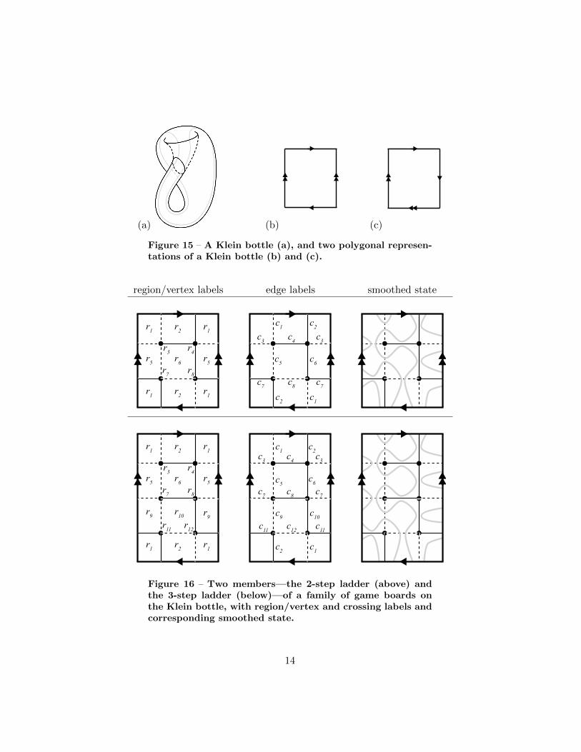
So far, we’ve focused on game boards that live on the surface of asphere, but some of the most interesting examples of games we’ve comeacross live on more complex surfaces. In particular, there exists aninfinite family of game boards on the Klein bottle on which Player Chas a winning strategy moving second. Before we describe our gameboard, let us recall one useful method of representing the Klein bottle:as a square with certain edges identified. In Figure 15, we see a popularrepresentation of a Klein bottle (from Wikipedia) together with twopossible polygonal representations, where edges are identified in pairsaccording to the orientations shown in the diagram.

To picture a family of game boards on the Klein bottle that wecall the “ladder family,” we make use of the polygonal representationin Figure 15(b). The two smallest members of this family, n = 2 (the2-step ladder) and n = 3 (the 3-step ladder), are shown in Figure 16.We will refer to the horizontal graph edges as the “steps” of the ladderand the vertical edges as the “rails.”

Unlike game play on the sphere, notice that it is possible for asmoothed state on the Klein bottle to be connected when the selectedsubgraph contains a cycle. For example, the smoothed states in Fig-ure 16 are connected, but the graphs contain a cycle. Before furtherdiscussion of the game, we make an observation about special gameboards, like those in Figure 16, that contain a cycle and always resultin a connected smoothed state.

13

(a) (b) (c)

Figure 15 – A Klein bottle (a), and two polygonal represen-tations of a Klein bottle (b) and (c).

region/vertex labels edge labels smoothed state

r1

r2

r1

r5

r6

r5

r1

r2

r1

r3

r4

r7

r8

c3

c4

c5

c6

c7

c8

c2

c1

c3

c7

c2

c1

r1

r2

r1

r5

r6

r5

r1

r2

r1

r3

r4

r7

r8

r9

r10

r9

r11

r12

c1

c2

c3

c4

c3

c5

c6

c7

c8

c7

c9

c10

c11

c12

c11

c2

c1

Figure 16 – Two members—the 2-step ladder (above) andthe 3-step ladder (below)—of a family of game boards onthe Klein bottle, with region/vertex and crossing labels andcorresponding smoothed state.

14

Lemma 5. If a subgraph of an n-step ladder graph on the Klein bottlecontains exactly one horizontal step and exactly one rail at each heightof the ladder, then the smoothed state corresponding to this subgraphis connected.

Proof. We begin by making a quick observation regarding a simplesubgraph of the n-step ladder graph. Then we prove the lemma for anarbitrary subgraph of the ladder that contains exactly one horizontalstep and exactly one rail at each height.

The simple subgraph we consider first is the graph that containsthe edges c2, c6, . . . , c4n−2 and c4n. For the 3-step ladder, this graph isin Figure 17(a). Observe that an ε-neighborhood of this graph withinthe Klein bottle is a Mobius strip, therefore the boundary of this ε-neighborhood consists of exactly one connected component. Also no-tice that if smoothings were made around this graph they would traceout the boundary of the Mobius strip, thus one smoothed componentwould surround this graph.

Figure 17 – (a) A simple graph with ε-neighborhood home-omorphic to a Mobius strip. (b-c) Examples of subgraphsof the ladder graph that contain exactly one horizontal stepand exactly one rail at each height of the ladder.

To prove Lemma 5, we consider an arbitrary subgraph, G, of theladder that contains exactly one horizontal step and exactly one rail ateach height. Since the graph contains exactly one step at each height,it cannot contain any vertices of degree four or zero. Thus, G can onlycontain vertices of degree one, two, or three, as shown in Figure 17(b)& (c). In particular, this implies that every vertex is included in G.

Since G contains a single rail at each height, each step of G will ei-ther have a rail on each end or two rails on one end of the step. Thus,each step in G will either have both adjacent vertices of degree twoor the step will have vertices of degree three and one. We create an

15

ε-neighborhood around the subgraph G′ of G that contains every railof G and each step of G whose adjacent vertices are both degree two.Using an inductive argument starting at the bottom of the ladder, thissubgraph can be viewed as a non-decreasing path up the ladder thatconnects up exactly once along the orientation-reversing identificationson the bottom and top of the polygon. If the ε-neighborhood aroundthe subgraph G′ is glued along all orientation-preserving identifica-tions within G′, we get a connected rectangular strip with orientation-reversing gluings at each end. Therefore, the ε-neighborhood aroundthe subgraph G′ is homeomorphic to a Mobius strip. As in the caseof the simple graph, smoothings made in the diagram according to theedges in G′ will result in a single boundary component around G′.

To complete the argument for G, we notice that the only edges inG that are not in G′ are the degree three and one vertices. Thus, thegraph G′ is a connected strong deformation retract of G via the homo-topy that continuously shrinks each step in G−G′ towards the degreethree vertex of that step. This simple homotopy can be extended tothe ε-neighborhood of G to prove that the ε-neighborhood of G′ is astrong deformation retract of the ε-neighborhood of G. Following thishomotopy on ε-neighborhoods, the smoothed state corresponding tothe graph G is isotopic to the smoothed state corresponding to G′.Therefore, the smoothed state corresponding to G is one connectedcomponent.

Theorem 6. If Player C moves second, then Player C has a winningstrategy playing the Region Smoothing Swap Game on any game boardassociated to ladder family of links on the Klein bottle that containsexactly one horizontal step and exactly one rail at each height of theladder (such as the game boards shown in Figure 16).

Proof. First, following Lemma 5, we note that our goal is to produce asubgraph of the checkerboard graph that contains exactly one rail andexactly one step at each height. Our starting configuration has thisproperty. For the game on this graph, we follow a pairing strategy,setting ε2i−1 = ε2i (see labelings in Figure 16) so Player C will mimicD’s moves in these pairs.

First of all, if Player D chooses ε2i−1 = 0 or ε2i = 0 for some i, ourmimicking strategy preserves the status quo—our graph is unaltered.Suppose, then, that Player D chooses ε2i−1 = 1 or ε2i = 1 for some i.Then Player C will ensure ε2i−1 = ε2i = 1. In the diagram that resultsfrom this pair of moves, neither edge c2i−1 or c2i has been altered, butfour edges have been switched, namely c2i−3, c2i−2, c2i+1, and c2i+2

(with subscripts mod 4n for the n-step ladder). If exactly one of theedges c2i−3 and c2i−2 was initially in the (bold) subgraph, then exactlyone edge will be in the subgraph following the two moves. Similarly

16

for c2i+1 and c2i+2. Thus, our desired “one edge at each height” prop-erty has been preserved, and the final game board is connected, byLemma 5.

5 Game Play on the Connect Sum of TwoKlein Bottles

We’ve just seen an interesting game board on a Klein bottle, but whystop there? Are there game boards on more complex surfaces for whichPlayer C has a winning strategy? We asked just this question and foundan intriguing example on the connect sum of two Klein bottles.

r1

r2

r3

r4

r5

r8

r6

r7

c1

c2

c3

c2

c3

c8

c7

c3

c8

c10

c4

c10

c4

c1

c7

c4

c5

c6

c9

Figure 18 – A graph on the connect sum of two Klein bottles,with labels.

The matrix corresponding to this example is as follows, where theith column corresponds to ci and the jth row corresponds to rj .

17

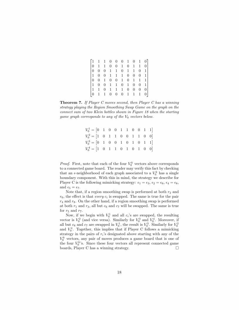
1 1 1 0 0 0 1 0 1 00 1 1 0 0 1 0 1 1 00 0 0 1 1 0 1 1 0 11 0 0 1 1 1 0 0 0 10 0 1 0 0 1 0 1 1 11 0 0 1 1 0 1 0 0 11 1 0 1 1 1 0 0 0 00 1 1 0 0 0 1 1 1 0

Theorem 7. If Player C moves second, then Player C has a winningstrategy playing the Region Smoothing Swap Game on the graph on theconnect sum of two Klein bottles shown in Figure 18 when the startinggame graph corresponds to any of the V0 vectors below.

V 10 =

[0 1 0 0 1 1 0 0 1 1

]V 20 =

[1 0 1 1 0 0 1 1 0 0

]V 30 =

[0 1 0 0 1 0 1 0 1 1

]V 40 =

[1 0 1 1 0 1 0 1 0 0

]Proof. First, note that each of the four V k

0 vectors above correspondsto a connected game board. The reader may verify this fact by checkingthat an ε-neighborhood of each graph associated to a V k

0 has a singleboundary component. With this in mind, the strategy we describe forPlayer C is the following mimicking strategy: ε1 = ε3, ε2 = ε6, ε4 = ε8,and ε5 = ε7.

Note that, if a region smoothing swap is performed at both r2 andr6, the effect is that every ci is swapped. The same is true for the pairr4 and r8. On the other hand, if a region smoothing swap is performedat both r1 and r3, all but c6 and c7 will be swapped. The same is truefor r5 and r7.

Now, if we begin with V 10 and all ci’s are swapped, the resulting

vector is V 20 (and vice versa). Similarly for V 3

0 and V 40 . Moreover, if

all but c6 and c7 are swapped in V 10 , the result is V 3

0 . Similarly for V 20

and V 40 . Together, this implies that if Player C follows a mimicking

strategy in the pairs of ri’s designated above starting with any of theV k0 vectors, any pair of moves produces a game board that is one of

the four V k0 ’s. Since these four vectors all represent connected game

boards, Player C has a winning strategy.

18

6 Related Results

As we discussed in the introduction, the Region Smoothing Swap Gameis a variation on the Link Smoothing Game. In [2], game boards werepartially classified according to their outcome classes. Here, we providea proof of completing the classification of Link Smoothing game boards.

Theorem 8. Let G be a connected, planar graph associated to a linkshadow D. If G represents a P-position game (i.e., a game in whichthe second player has a winning strategy), then G is composed of twoedge-disjoint spanning trees.

To prove the theorem, we use a result of Nash-Williams [3] andseparately Tutte [4], that gives a necessary and sufficient condition fora graph G to have two edge-disjoint spanning trees. Before statingthe conditions, though, we need some notation for a special graphassociated to G that is defined in terms of a partition of the vertex setof G.

Let G be a graph with vertex set V (G) and edge set E(G). Wedenote the number of vertices and edges in G by |V (G)| and |E(G)|respectively. For a partition P of V (G), we define EP (G) as the setof edges that join vertices belonging to different members of P . Thegraph GP is defined as the graph with vertex set P and edge set EP (G).The Nash-Williams and Tutte result can now be stated as follows.

Theorem 9 (Nash-Williams, Tutte). A graph G has k edge-disjointspanning trees if and only if

|EP (G)| ≥ k(|P | − 1)

for every partition P of V (G).

Proof of Theorem 8. We begin with the supposition that G is a P -position graph for the link smoothing game. The definition of P -position implies that the player with the goal to keep the diagramconnected has a winning strategy when moving second on the givengame board. Such a winning strategy can only exist if there are aneven number of edges in the graph G, else the player moving last wouldbe the player with goal to disconnect and such a player can always dis-connect the diagram on the final move.

By way of contradiction, we suppose that G does not consist of twoedge disjoint spanning trees. Then the result of Nash-Williams andTutte implies the existence of a partition P of the vertices of G suchthat |EP (G)| < 2(|P |−1). Since the set EP (G) is a subset of the edgesof G and |P | is less than |V (G)|, we can conclude |E(G)| ≤ |EP (G)| <2(|P | − 1) ≤ 2(|V (G)| − 1). Hence,

|E(G)| < 2(|V (G)| − 1).

19

By Theorem 6 in [2], the previous inequality implies the graph repre-sents an L-position diagram. This contradicts our P -position supposi-tion.

7 Questions for Further Research

In doing research on the Region Smoothing Swap Game, our goal hasbeen to find examples of link diagrams on surfaces on which Player Chas a winning strategy. Since Player D tends to have an advantage inthis game, finding such examples can be challenging. What is specialabout examples for which Player C has a winning strategy? An analysisakin to the one begun for the Link Smoothing Game in [2] which wascompleted in Section 6 above would be interesting. Such an analysiswill likely be more challenging to perform, however, in the setting ofthe Region Smoothing Swap Game on surfaces. It would be especiallyinteresting to know more about the relationship between examples onwhich C can win and the surfaces on which these link smoothings live.

This topic provides a wealth of other open problems for those whoare curious about variations on the Region Smoothing Swap Game.Just as with the Link Smoothing Game, the players’ goals can bechanged or the allowable moves can be modified to create a new gameto study. We encourage our readers to invent and study their owngames with knots, links, graphs, and surfaces!

8 Acknowledgements.

The authors would like to thank the Simons Foundation (#426566,Allison Henrich) for their support of this research.

References

[1] S. Brown, F. Cabrera, R. Evans, G. Gibbs, A. Henrich and J.Kreinbihl, The region unknotting game. Math. Mag. 90 no. 5(2017) 323-337.

[2] A. Henrich and I. Johnson, The link smoothing game. AKCE Int.J. Graphs Comb. 9 no. 2 (2012) 145-159.

[3] C. St.J. A. Nash-Williams, Edge-Disjoint Spanning Trees of FiniteGraphs. Journal London Math. Soc. 36 (1961) 445–450.

[4] W. T. Tutte, On the problem of decomposing a graph into nconnected factors. Journal London Math. Soc. 142 (1961), 221–230.

20