the reconstruction of large three ...misha/bolitho/thesis.pdfabstract based on the solution to a...
TRANSCRIPT
THE RECONSTRUCTION OF LARGE
THREE-DIMENSIONAL MESHES
by
Matthew Grant Bolitho
A dissertation submitted to The Johns Hopkins University in conformity with
the requirements for the degree of Doctor of Philosophy.
Baltimore, Maryland
March, 2010
c© Matthew Grant Bolitho 2010
All rights reserved
Abstract
Surface reconstruction is the process of creating virtual three-dimensional
representations of real-world objects using data obtained from 3D scanners.
The traditional challenges of surface reconstruction arise from the uncertain
nature of input data. Inaccuracies in scanning devices create noisy data.
Point sampling is often non-uniform. And, accessibility constraints during the
scanning process may leave some regions of the surface devoid of data. Robustly
constructing a surface in the presence of these data anomalies is a difficult problem.
In addition, surface reconstruction methods have recently encountered a new
challenge resulting from developments in 3D scanning techniques. New scanning
technologies have driven a dramatic increase in the size of datasets available for
surface reconstruction, with datasets now exceeding one billion point samples.
As a result, space and time efficiency have become critical in the development
of effective reconstruction algorithms, and the design of streaming and parallel
techniques has become indispensable.
In this dissertation we describe a new technique for surface reconstruction,
ii
ABSTRACT
based on the solution to a Poisson equation. Our approach is designed to meet
the multiple challenges of modern datasets. The method is robust to the types of
noise found in real-world data, allowing the reconstruction of high quality surfaces.
Despite formulating surface reconstruction as a global problem, we also show that
our method can be implemented using only local updates which allows extremely
large reconstruction problems to be solved in a streaming manner. We also exploit
current industry trends towards multi-core and parallel computing by presenting a
parallel implementation of our method that is able to dramatically reduce the time
taken to produce highly detailed reconstructions. We demonstrate the practicality
of our method on several of the largest reconstruction datasets available to date.
Primary Reader: Dr. Michael Kazhdan
Secondary Readers: Dr. Randal Burns and Dr. Szymon Rusinkiewicz
iii

Acknowledgements
iv

Dedication
v
Contents
Abstract ii
Acknowledgements iv
List of Tables xii
List of Figures xiv
1 Introduction 1
1.1 3D Scanning . . . . . . . . . . . . . . . . . . . . . . . . . . . . . . 2
1.2 Surface Reconstruction . . . . . . . . . . . . . . . . . . . . . . . . 5
1.3 Outline of Dissertation . . . . . . . . . . . . . . . . . . . . . . . . 10
2 Surface Reconstruction 11
2.1 Discrete Methods . . . . . . . . . . . . . . . . . . . . . . . . . . . 14
2.1.1 Computational Geometry . . . . . . . . . . . . . . . . . . 14
2.1.2 Alpha Shapes . . . . . . . . . . . . . . . . . . . . . . . . . 14
vi
CONTENTS
2.1.3 Power Crust . . . . . . . . . . . . . . . . . . . . . . . . . . 15
2.1.4 Ball Pivoting . . . . . . . . . . . . . . . . . . . . . . . . . 16
2.2 Continuous Methods . . . . . . . . . . . . . . . . . . . . . . . . . 17
2.2.1 Surface Fitting . . . . . . . . . . . . . . . . . . . . . . . . 17
2.2.1.1 Balloon Fitting . . . . . . . . . . . . . . . . . . . 17
2.2.1.2 Fast Level Set Method . . . . . . . . . . . . . . . 18
2.2.1.3 Point Set Surfaces . . . . . . . . . . . . . . . . . 18
2.2.2 Implicit Function Fitting . . . . . . . . . . . . . . . . . . . 19
2.2.3 Local Function Fitting . . . . . . . . . . . . . . . . . . . . 20
2.2.3.1 Hoppe et al. . . . . . . . . . . . . . . . . . . . . . 20
2.2.3.2 Volumetric Range Image Processing (VRIP) . . . 21
2.2.3.3 Multi-level Partitions of Unity (MPU) . . . . . . 22
2.2.4 Global Function Fitting . . . . . . . . . . . . . . . . . . . 23
2.2.4.1 Blobby Models . . . . . . . . . . . . . . . . . . . 23
2.2.4.2 Fast RBF . . . . . . . . . . . . . . . . . . . . . . 24
2.2.4.3 Fast Fourier Transform . . . . . . . . . . . . . . . 26
2.2.4.4 Wavelets . . . . . . . . . . . . . . . . . . . . . . . 27
2.2.4.5 Our Approach . . . . . . . . . . . . . . . . . . . 28
3 Poisson Surface Reconstruction 29
3.1 The Poisson Idea . . . . . . . . . . . . . . . . . . . . . . . . . . . 29
3.2 Approach . . . . . . . . . . . . . . . . . . . . . . . . . . . . . . . 32
vii
CONTENTS
3.2.1 Defining the gradient field . . . . . . . . . . . . . . . . . . 33
3.2.2 Approximating the gradient field . . . . . . . . . . . . . . 34
3.2.3 Solving the Poisson problem . . . . . . . . . . . . . . . . . 35
3.3 Implementation . . . . . . . . . . . . . . . . . . . . . . . . . . . . 36
3.3.1 Problem Discretization . . . . . . . . . . . . . . . . . . . . 37
3.3.1.1 Defining the function space . . . . . . . . . . . . 38
3.3.1.2 Selecting a base function . . . . . . . . . . . . . . 39
3.3.2 Vector Field Definition . . . . . . . . . . . . . . . . . . . . 40
3.3.3 Linear System Definition . . . . . . . . . . . . . . . . . . . 41
3.3.4 Iso-Surface Extraction . . . . . . . . . . . . . . . . . . . . 43
3.3.5 Non-uniform Samples . . . . . . . . . . . . . . . . . . . . . 44
3.3.5.1 Estimating local sampling density . . . . . . . . . 45
3.3.5.2 Estimating a samples depth . . . . . . . . . . . . 47
3.3.5.3 Computing the vector field . . . . . . . . . . . . 47
3.3.6 Selecting an iso-value . . . . . . . . . . . . . . . . . . . . . 49
3.4 Results . . . . . . . . . . . . . . . . . . . . . . . . . . . . . . . . . 49
3.4.1 Resilience to Noise . . . . . . . . . . . . . . . . . . . . . . 50
3.4.2 Comparison to Previous Work . . . . . . . . . . . . . . . . 52
3.4.2.1 Comparison to Wavelet-based approach . . . . . 54
3.4.2.2 Comparison to the FFT-based approach . . . . . 56
3.4.2.3 Comparison to VRIP . . . . . . . . . . . . . . . . 57
viii
CONTENTS
3.4.2.4 Limitation of our approach . . . . . . . . . . . . 58
3.4.3 Performance and Scalability . . . . . . . . . . . . . . . . . 60
4 Streaming Surface Reconstruction 64
4.1 Related Work . . . . . . . . . . . . . . . . . . . . . . . . . . . . . 67
4.1.1 Out-of-core Surface Reconstruction . . . . . . . . . . . . . 67
4.1.2 Stream Processing . . . . . . . . . . . . . . . . . . . . . . 68
4.1.3 Other Out-of-core Processing . . . . . . . . . . . . . . . . 68
4.1.4 Out-of-core Linear Solvers . . . . . . . . . . . . . . . . . . 69
4.2 Representation . . . . . . . . . . . . . . . . . . . . . . . . . . . . 69
4.2.1 Implementation . . . . . . . . . . . . . . . . . . . . . . . . 72
4.3 A Simple Streaming Reconstruction . . . . . . . . . . . . . . . . . 74
4.3.1 Pre-processing . . . . . . . . . . . . . . . . . . . . . . . . . 76
4.3.2 Octree Construction (k = 1) . . . . . . . . . . . . . . . . . 77
4.3.3 Vector Field Construction (k = 1) . . . . . . . . . . . . . . 77
4.3.4 Divergence Computation (k = 2) . . . . . . . . . . . . . . 78
4.3.5 Poisson System Solution (k = 2) . . . . . . . . . . . . . . . 81
4.3.6 Computing the Iso-Value (k = 1) . . . . . . . . . . . . . . 82
4.3.7 Extracting the Iso-Surface (k = 2) . . . . . . . . . . . . . . 82
4.4 An Optimized Implementation . . . . . . . . . . . . . . . . . . . . 86
4.4.1 First Pass (k = 6) . . . . . . . . . . . . . . . . . . . . . . . 87
4.4.1.1 Buffering Samples . . . . . . . . . . . . . . . . . 88
ix
CONTENTS
4.4.2 Second Pass (k = 8) . . . . . . . . . . . . . . . . . . . . . 89
4.4.2.1 Index Dependencies . . . . . . . . . . . . . . . . 90
4.4.2.2 Depth Dependencies . . . . . . . . . . . . . . . . 90
4.5 Results . . . . . . . . . . . . . . . . . . . . . . . . . . . . . . . . . 91
4.5.1 Large Datasets . . . . . . . . . . . . . . . . . . . . . . . . 91
4.5.2 Scalable Memory Use . . . . . . . . . . . . . . . . . . . . . 93
4.5.3 Computation Times . . . . . . . . . . . . . . . . . . . . . 98
4.5.4 Streaming Solver Accuracy . . . . . . . . . . . . . . . . . . 100
4.6 Discussion . . . . . . . . . . . . . . . . . . . . . . . . . . . . . . . 100
5 Parallel Surface Reconstruction 105
5.1 Related Work . . . . . . . . . . . . . . . . . . . . . . . . . . . . . 107
5.2 Parallel Reconstruction . . . . . . . . . . . . . . . . . . . . . . . . 108
5.3 Shared Memory . . . . . . . . . . . . . . . . . . . . . . . . . . . . 108
5.3.1 Data Partitioning . . . . . . . . . . . . . . . . . . . . . . . 109
5.3.2 Work Distribution . . . . . . . . . . . . . . . . . . . . . . 110
5.3.3 Data Sharing . . . . . . . . . . . . . . . . . . . . . . . . . 112
5.3.3.1 Tree Construction . . . . . . . . . . . . . . . . . 115
5.3.3.2 Solving the Laplacian . . . . . . . . . . . . . . . 116
5.3.4 Scalability Issues . . . . . . . . . . . . . . . . . . . . . . . 117
5.4 Distributed Memory . . . . . . . . . . . . . . . . . . . . . . . . . 120
5.4.1 Data Partitioning . . . . . . . . . . . . . . . . . . . . . . . 121
x
CONTENTS
5.4.2 Load Balancing . . . . . . . . . . . . . . . . . . . . . . . . 123
5.4.3 Replication and Merging of Shared Data . . . . . . . . . . 123
5.4.4 Tree Construction . . . . . . . . . . . . . . . . . . . . . . . 125
5.4.5 Solving the Laplacian . . . . . . . . . . . . . . . . . . . . . 126
5.5 Results . . . . . . . . . . . . . . . . . . . . . . . . . . . . . . . . . 127
5.5.1 Correctness . . . . . . . . . . . . . . . . . . . . . . . . . . 128
5.5.2 Skew . . . . . . . . . . . . . . . . . . . . . . . . . . . . . . 129
5.5.3 Scalability . . . . . . . . . . . . . . . . . . . . . . . . . . . 131
5.5.4 David . . . . . . . . . . . . . . . . . . . . . . . . . . . . . 134
6 Conclusion 137
6.1 Future Work . . . . . . . . . . . . . . . . . . . . . . . . . . . . . . 140
6.1.1 A GPU Implementation . . . . . . . . . . . . . . . . . . . 140
6.1.2 A Surface Reconstruction Benchmark . . . . . . . . . . . . 141
Bibliography 144
Vita 154
xi
List of Tables
3.1 The running time (in seconds), the peak memory usage (inmegabytes), and the number of triangles in the reconstructed modelfor the different depth reconstructions of the Dragon model. Akernel depth of 6 was used for density estimation. . . . . . . . . . 61
3.2 The running time (in seconds), the peak memory usage (inmegabytes), and the number of triangles in the reconstructedsurface of the Stanford Bunny generated by the different methods. 63
4.1 Read and write operations when processing block Sdi in the various
multilevel streaming computations. . . . . . . . . . . . . . . . . . 764.2 Quantitative results for multilevel streaming reconstructions,
showing input points, octree height D + 1, output mesh triangles,total execution time (hours), memory use (MB), and total octreestream size (MB). . . . . . . . . . . . . . . . . . . . . . . . . . . . 92
4.3 Comparison of the data structure size (MB), peak working set(MB), and running time (hours) for the in-core and streamingreconstruction algorithms over a range of resolutions for the DavidHead model. Running the in-core algorithm beyond a resolution of2048 was impossible due to its high memory requirements. . . . . 103
5.1 A summary of the the size of each output model, and the maximumand average vertex distance from the serial output of severaldifferent reconstructions of the Bunny dataset at depth 9 createdwith the distributed implementation. . . . . . . . . . . . . . . . . 127
xii
LIST OF TABLES
5.2 The running time (in minutes), aggregate disk use (in MB),and peak memory use (in MB) of the shared memory anddistributed memory implementations of the Parallel PoissonSurface Reconstruction algorithms for the Lucy dataset at depth12, with dfull = 6 and the David dataset at depth 14 with dfull = 8,running on one through twelve processors. It was not possibleto run the shared memory implementation on more than eightprocessors. . . . . . . . . . . . . . . . . . . . . . . . . . . . . . . 131
xiii
List of Figures
1.1 Four examples of reconstructed objects from different disciplines. . 31.2 An example of the reconstruction of the “Bunny” model. Individual
scans of the real object are first aligned and combined before asurface reconstruction algorithm produces the final model. . . . . 5
1.3 Illustrative examples of the different types of data anomaliespresent in three-dimensional scan data: a) noise, b) anisotropy,c) misalignment, d) non-uniformity, and e) missing data. . . . . . 6
1.4 Two examples showing how multiple types of anomalies combinein real-world data. . . . . . . . . . . . . . . . . . . . . . . . . . . 9
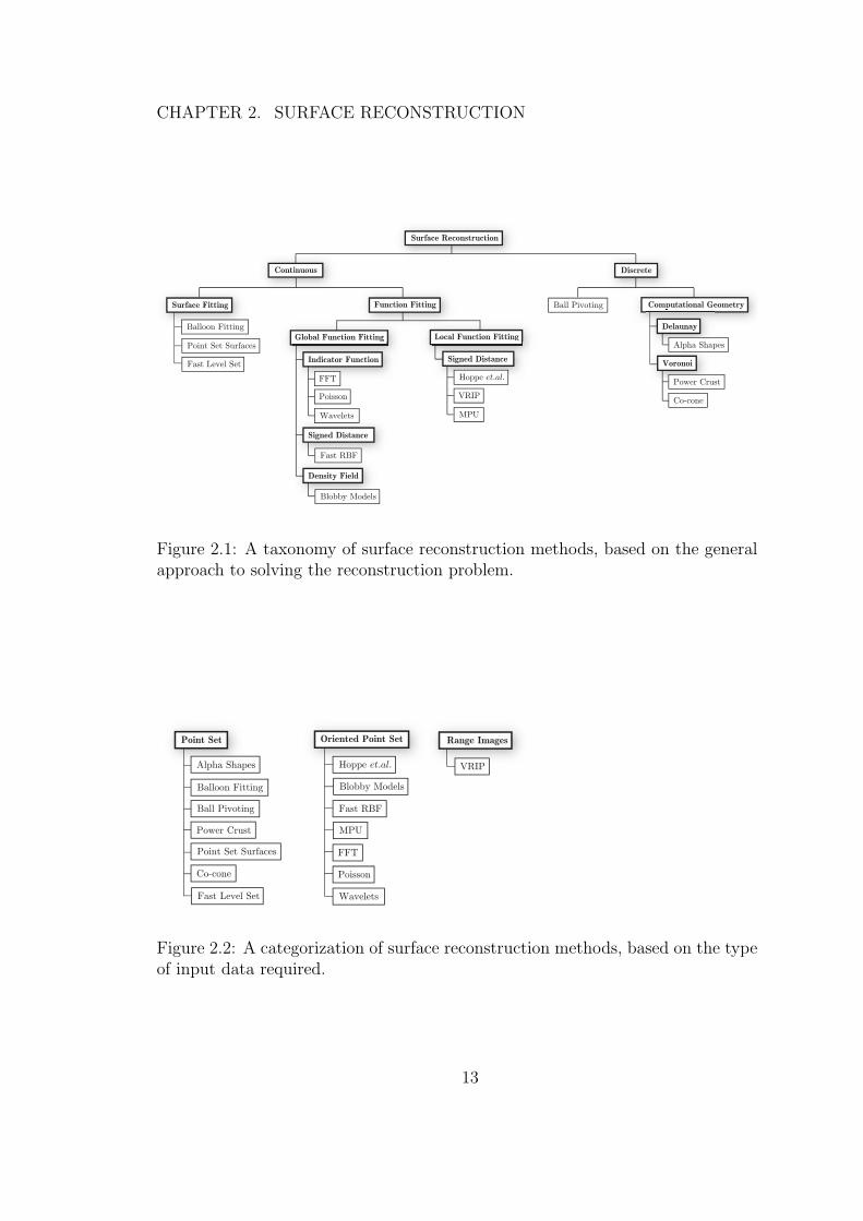
2.1 A taxonomy of surface reconstruction methods, based on thegeneral approach to solving the reconstruction problem. . . . . . . 13
2.2 A categorization of surface reconstruction methods, based on thetype of input data required. . . . . . . . . . . . . . . . . . . . . . 13
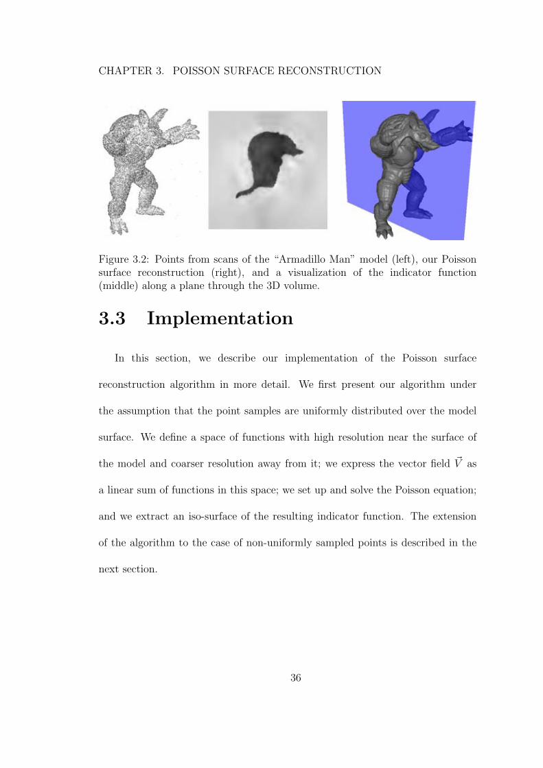
3.1 Intuitive illustration of Poisson reconstruction in 2D. . . . . . . . 303.2 Points from scans of the “Armadillo Man” model (left), our Poisson
surface reconstruction (right), and a visualization of the indicatorfunction (middle) along a plane through the 3D volume. . . . . . 36
3.3 A comparison of the reconstruction of a highly non-uniform datasetusing a low resolution (b), high resolution (c) and adaptiveresolution sample density estimation (d). . . . . . . . . . . . . . . 46
3.4 Reconstructions of an 200,000 point sampling of the “ArmadilloMan” model at depth 9 with varying amounts of random noiseintroduced to the position (δ) and normal (θ) component to thesamples. r is the radius of the models bounding sphere. . . . . . . 51
3.5 Reconstructions of the Stanford Bunny using Power Crust (a),Robust Cocone (b), Fast RBF (c), MPU (d), Hoppe et al.’sreconstruction (e), Wavelet-based reconstruction (f), FFT-basedreconstruction (g), VRIP (h), and our Poisson reconstruction (i). . 53
xiv
LIST OF FIGURES
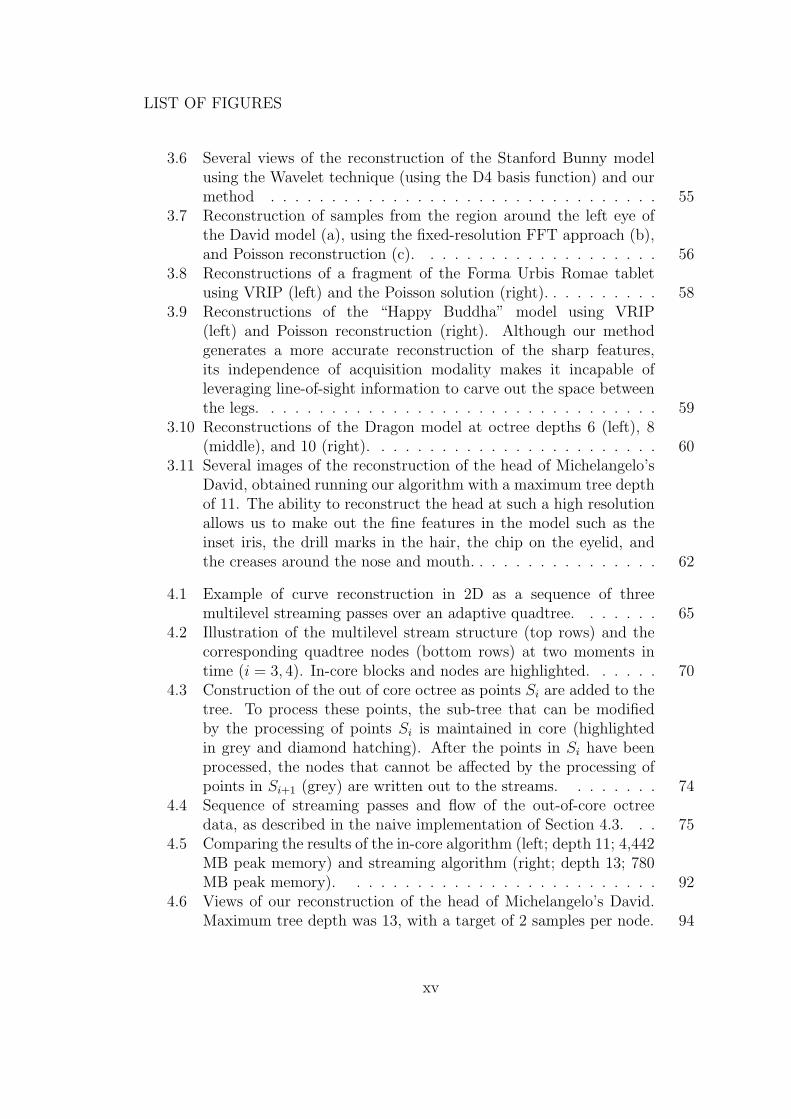
3.6 Several views of the reconstruction of the Stanford Bunny modelusing the Wavelet technique (using the D4 basis function) and ourmethod . . . . . . . . . . . . . . . . . . . . . . . . . . . . . . . . 55
3.7 Reconstruction of samples from the region around the left eye ofthe David model (a), using the fixed-resolution FFT approach (b),and Poisson reconstruction (c). . . . . . . . . . . . . . . . . . . . 56
3.8 Reconstructions of a fragment of the Forma Urbis Romae tabletusing VRIP (left) and the Poisson solution (right). . . . . . . . . . 58
3.9 Reconstructions of the “Happy Buddha” model using VRIP(left) and Poisson reconstruction (right). Although our methodgenerates a more accurate reconstruction of the sharp features,its independence of acquisition modality makes it incapable ofleveraging line-of-sight information to carve out the space betweenthe legs. . . . . . . . . . . . . . . . . . . . . . . . . . . . . . . . . 59
3.10 Reconstructions of the Dragon model at octree depths 6 (left), 8(middle), and 10 (right). . . . . . . . . . . . . . . . . . . . . . . . 60
3.11 Several images of the reconstruction of the head of Michelangelo’sDavid, obtained running our algorithm with a maximum tree depthof 11. The ability to reconstruct the head at such a high resolutionallows us to make out the fine features in the model such as theinset iris, the drill marks in the hair, the chip on the eyelid, andthe creases around the nose and mouth. . . . . . . . . . . . . . . . 62
4.1 Example of curve reconstruction in 2D as a sequence of threemultilevel streaming passes over an adaptive quadtree. . . . . . . 65
4.2 Illustration of the multilevel stream structure (top rows) and thecorresponding quadtree nodes (bottom rows) at two moments intime (i = 3, 4). In-core blocks and nodes are highlighted. . . . . . 70
4.3 Construction of the out of core octree as points Si are added to thetree. To process these points, the sub-tree that can be modifiedby the processing of points Si is maintained in core (highlightedin grey and diamond hatching). After the points in Si have beenprocessed, the nodes that cannot be affected by the processing ofpoints in Si+1 (grey) are written out to the streams. . . . . . . . 74
4.4 Sequence of streaming passes and flow of the out-of-core octreedata, as described in the naive implementation of Section 4.3. . . 75
4.5 Comparing the results of the in-core algorithm (left; depth 11; 4,442MB peak memory) and streaming algorithm (right; depth 13; 780MB peak memory). . . . . . . . . . . . . . . . . . . . . . . . . . 92
4.6 Views of our reconstruction of the head of Michelangelo’s David.Maximum tree depth was 13, with a target of 2 samples per node. 94
xv
LIST OF FIGURES
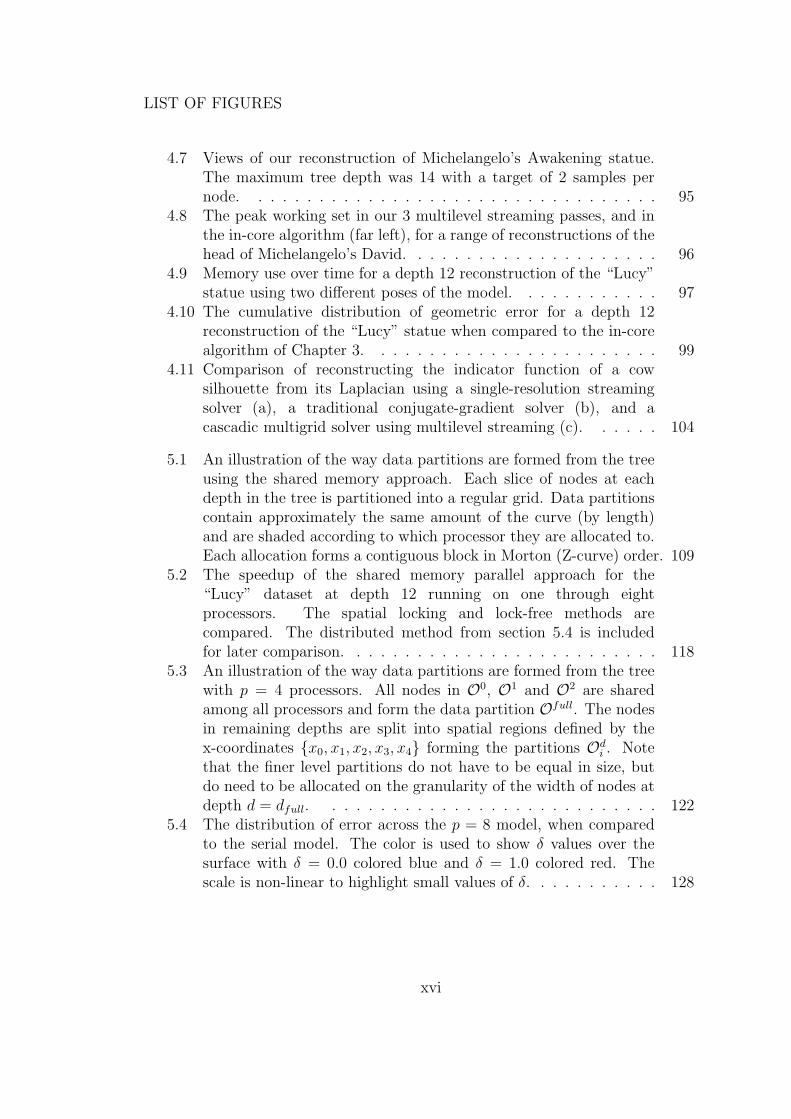
4.7 Views of our reconstruction of Michelangelo’s Awakening statue.The maximum tree depth was 14 with a target of 2 samples pernode. . . . . . . . . . . . . . . . . . . . . . . . . . . . . . . . . . 95
4.8 The peak working set in our 3 multilevel streaming passes, and inthe in-core algorithm (far left), for a range of reconstructions of thehead of Michelangelo’s David. . . . . . . . . . . . . . . . . . . . . 96
4.9 Memory use over time for a depth 12 reconstruction of the “Lucy”statue using two different poses of the model. . . . . . . . . . . . 97
4.10 The cumulative distribution of geometric error for a depth 12reconstruction of the “Lucy” statue when compared to the in-corealgorithm of Chapter 3. . . . . . . . . . . . . . . . . . . . . . . . 99
4.11 Comparison of reconstructing the indicator function of a cowsilhouette from its Laplacian using a single-resolution streamingsolver (a), a traditional conjugate-gradient solver (b), and acascadic multigrid solver using multilevel streaming (c). . . . . . 104
5.1 An illustration of the way data partitions are formed from the treeusing the shared memory approach. Each slice of nodes at eachdepth in the tree is partitioned into a regular grid. Data partitionscontain approximately the same amount of the curve (by length)and are shaded according to which processor they are allocated to.Each allocation forms a contiguous block in Morton (Z-curve) order. 109
5.2 The speedup of the shared memory parallel approach for the“Lucy” dataset at depth 12 running on one through eightprocessors. The spatial locking and lock-free methods arecompared. The distributed method from section 5.4 is includedfor later comparison. . . . . . . . . . . . . . . . . . . . . . . . . . 118
5.3 An illustration of the way data partitions are formed from the treewith p = 4 processors. All nodes in O0, O1 and O2 are sharedamong all processors and form the data partition Ofull. The nodesin remaining depths are split into spatial regions defined by thex-coordinates {x0, x1, x2, x3, x4} forming the partitions Od
i . Notethat the finer level partitions do not have to be equal in size, butdo need to be allocated on the granularity of the width of nodes atdepth d = dfull. . . . . . . . . . . . . . . . . . . . . . . . . . . . 122
5.4 The distribution of error across the p = 8 model, when comparedto the serial model. The color is used to show δ values over thesurface with δ = 0.0 colored blue and δ = 1.0 colored red. Thescale is non-linear to highlight small values of δ. . . . . . . . . . . 128
xvi

LIST OF FIGURES
5.5 The absolute value of the difference between the work allocatedto the processor with most work and the average, expressed as afunction of the height of the full resolution tree (dfull) and thenumber of processors. . . . . . . . . . . . . . . . . . . . . . . . . . 130
5.6 The speedup of the distributed implementation for the Lucy datasetat depth 12 and the David dataset at depth 14 running on onethrough twelve processors. The shared memory approach fromSection 5.3 in included for comparative purposes. . . . . . . . . . 132
5.7 A reconstruction of the David model at depth 15. . . . . . . . . . 135
xvii
Chapter 1
Introduction
Then this is enough to tell you what I mean by ‘shape’. For I say thisof every shape: a shape is that which limits a solid; in a word, a shapeis the limit of a solid. – Socrates to Meno, (Plato, Meno, 77)
One of the most fundamental concepts within the field of computer graphics is
shape. Any object seen in a computer-generated image, a scientific visualization,
a game or a movie is a shape with a virtual representation that is created,
manipulated and then rendered entirely within a computer.
Many representations of shape are used in computer graphics, ranging from
implicit mathematical formulations to the triangle mesh. A triangle mesh is a
discrete structure that represents a surface as a set of points in three-dimensional
space, connected in groups of three which form the triangular facets of a surface.
Although a surface represented in a discrete manner such as this cannot represent a
smooth surface, sufficiently small triangles can give an approximation of a smooth
1
CHAPTER 1. INTRODUCTION
surface that will be visually indistinguishable when viewed on a movie or computer
screen. Triangle meshes have become the most common representation for surfaces
primarily because the specialized computer hardware used to render interactive
3D scenes use this representation internally.
In the most basic setting, virtual representations of 3D models are created
manually, using modeling packages in which each vertex, edge or face in the mesh
is created and modified individually. Although this provides a high degree of
artistic freedom and works well for small models with thousands of triangles, the
ever-increasing demand for realism in computer-generated scenes has significantly
increased the model complexity, and therefore the time and cost of using these
techniques. New methods for generating models which can automate large parts
of the modeling process and reduce the amount of human interaction required
have become essential.
1.1 3D Scanning
The advent of 3D scanning techniques has significantly changed the way models
are created. Instead of using manual techniques to create virtual representations
of objects, real world objects can be scanned, providing an automated way of
generating highly detailed meshes.
In addition to improving the efficiency of 3D modelling, scanning technologies
2
CHAPTER 1. INTRODUCTION
a) Cuneiform Tablet c) Michelangelo's Davidb) Dental Scanning d) Turbine Blade
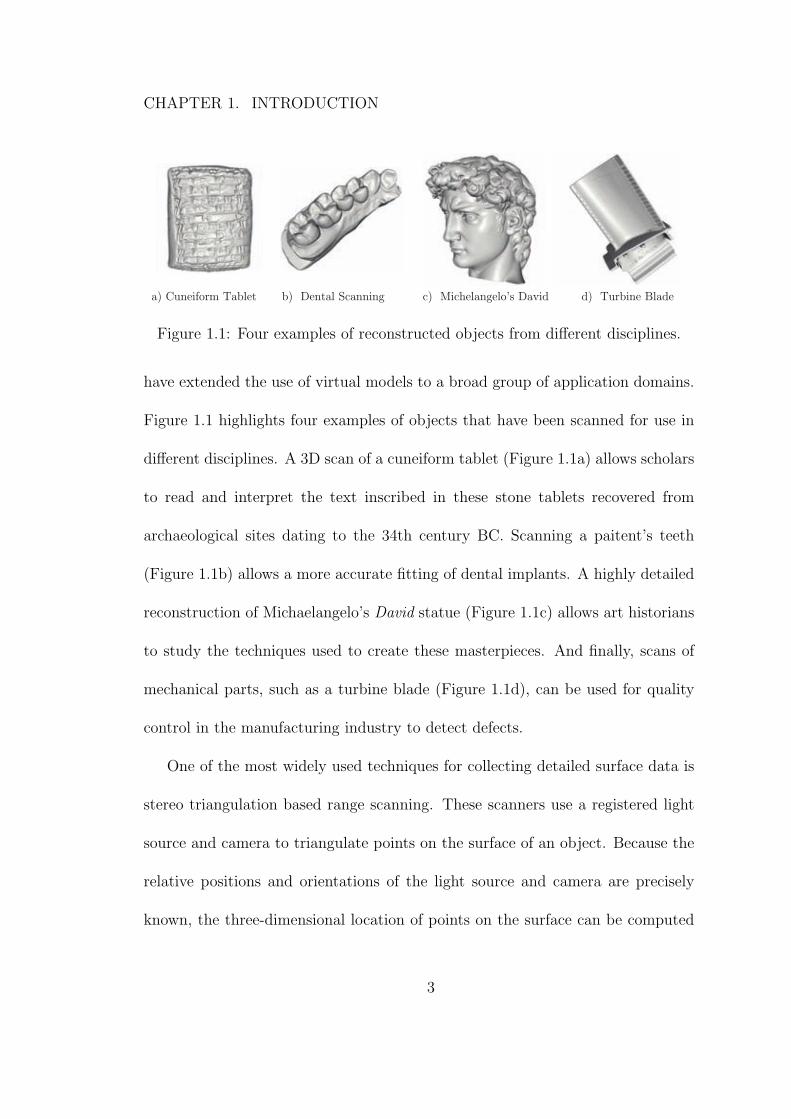
Figure 1.1: Four examples of reconstructed objects from different disciplines.
have extended the use of virtual models to a broad group of application domains.
Figure 1.1 highlights four examples of objects that have been scanned for use in
different disciplines. A 3D scan of a cuneiform tablet (Figure 1.1a) allows scholars
to read and interpret the text inscribed in these stone tablets recovered from
archaeological sites dating to the 34th century BC. Scanning a paitent’s teeth
(Figure 1.1b) allows a more accurate fitting of dental implants. A highly detailed
reconstruction of Michaelangelo’s David statue (Figure 1.1c) allows art historians
to study the techniques used to create these masterpieces. And finally, scans of
mechanical parts, such as a turbine blade (Figure 1.1d), can be used for quality
control in the manufacturing industry to detect defects.
One of the most widely used techniques for collecting detailed surface data is
stereo triangulation based range scanning. These scanners use a registered light
source and camera to triangulate points on the surface of an object. Because the
relative positions and orientations of the light source and camera are precisely
known, the three-dimensional location of points on the surface can be computed
3
CHAPTER 1. INTRODUCTION
by combining registration information and the location of features within the
camera’s image plane. Because of the reliance on triangulation, the accuracy of
these type of scanners decreases as the distance between the camera and the object
increases. In practice, however, they are capable of producing high quality scans
with sub-millimeter precision for objects within a range of several meters.
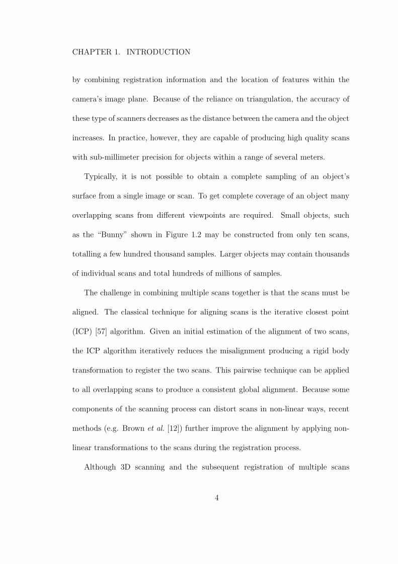
Typically, it is not possible to obtain a complete sampling of an object’s
surface from a single image or scan. To get complete coverage of an object many
overlapping scans from different viewpoints are required. Small objects, such
as the “Bunny” shown in Figure 1.2 may be constructed from only ten scans,
totalling a few hundred thousand samples. Larger objects may contain thousands
of individual scans and total hundreds of millions of samples.
The challenge in combining multiple scans together is that the scans must be
aligned. The classical technique for aligning scans is the iterative closest point
(ICP) [57] algorithm. Given an initial estimation of the alignment of two scans,
the ICP algorithm iteratively reduces the misalignment producing a rigid body
transformation to register the two scans. This pairwise technique can be applied
to all overlapping scans to produce a consistent global alignment. Because some
components of the scanning process can distort scans in non-linear ways, recent
methods (e.g. Brown et al. [12]) further improve the alignment by applying non-
linear transformations to the scans during the registration process.
Although 3D scanning and the subsequent registration of multiple scans
4
CHAPTER 1. INTRODUCTION
Aligned, Combined Scans Reconstructed ModelIndividual Scans
Figure 1.2: An example of the reconstruction of the “Bunny” model. Individualscans of the real object are first aligned and combined before a surfacereconstruction algorithm produces the final model.
provides high resolution geometry, it does not provide a fully connected mesh
of the surface: each scan is still represented as a separate patch of the surface.
For most uses, a single surface mesh is required.
1.2 Surface Reconstruction
Surface reconstruction is the process of the automated generation of three-
dimensional surfaces from a discrete sampling of the surface of a real object
acquired through 3D scanning. This can be an under-constrained process since the
reconstruction process must infer the shape between the samples, and there may
be many plausible surfaces that can be generated from any given set of samples.
5
CHAPTER 1. INTRODUCTION
a) c)
d)
?
e)
b)
Vie
w D
irec
tion
Low Density Low Density
Missing Data
High Density
Regularly Sampled Image Plane
Irregularly Sampled Surface
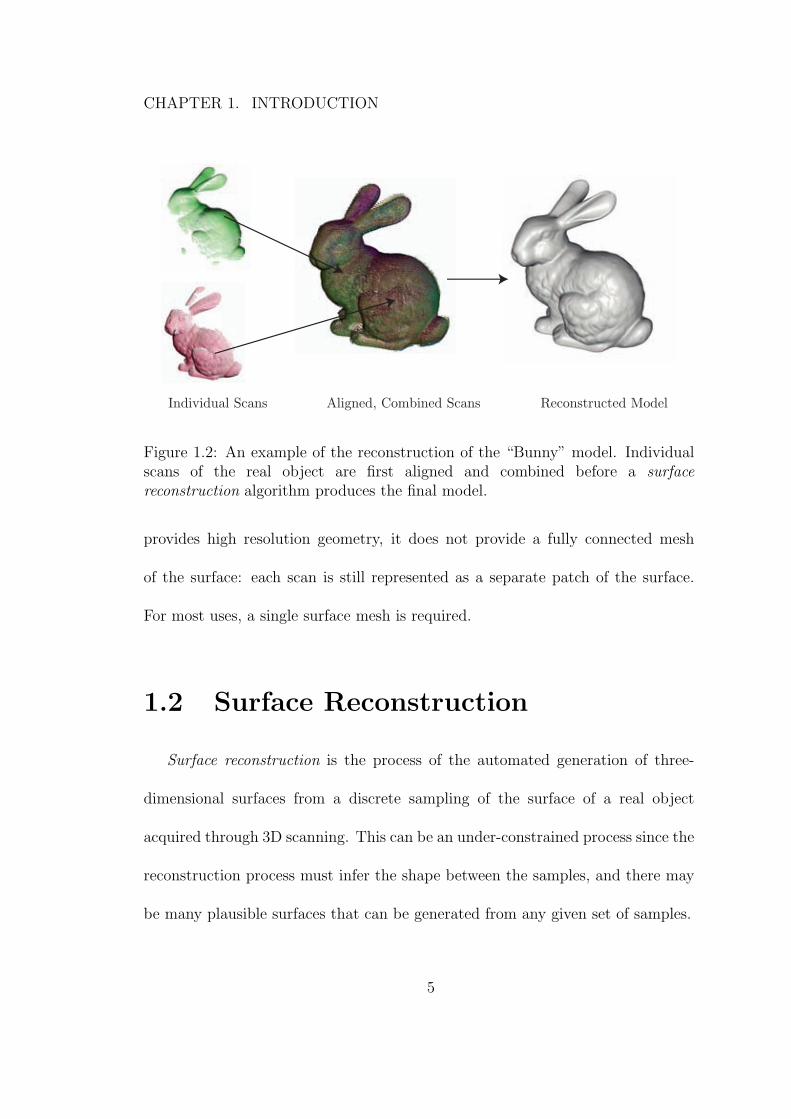
Figure 1.3: Illustrative examples of the different types of data anomalies presentin three-dimensional scan data: a) noise, b) anisotropy, c) misalignment, d) non-uniformity, and e) missing data.
One of the largest challenges in reconstructing surfaces robustly and accurately
is dealing with the many anomalies that are present in data that are obtained from
the scanning of real-world objects. There are many aspects to the data that make
the task of reconstruction particularly challenging.
• Noise: (Figure 1.3 a and b) The process of scanning involves capturing
measurements with an imaging device which, unavoidably, introduces noise
into all measurements. This noise manifests itself as uncertainty in the
positions of three-dimensional points or the orientation of surface normals
in the dataset. The level of noise is often variable and related to various
local characteristics of the surface (for example, reflectivity, or translucency)
and to the orientation of the surface in relation to the scanner (for example,
parts of the surface that are more oblique tend to have higher levels of noise).
• Misalignment: (Figure 1.3 c) When the samples are derived from multiple
6
CHAPTER 1. INTRODUCTION
scans, non-linear distortions and the lack of features in regions of scan
overlap can lead to imperfect alignment of scans. The consequence of scan
misalignment in the context of reconstruction is that the same patch of a
surface may be represented by multiple overlapping scans which disagree.
This often creates a situation where a single surface is represented in the
scan data as multiple “sheets” of samples, offset from each other.
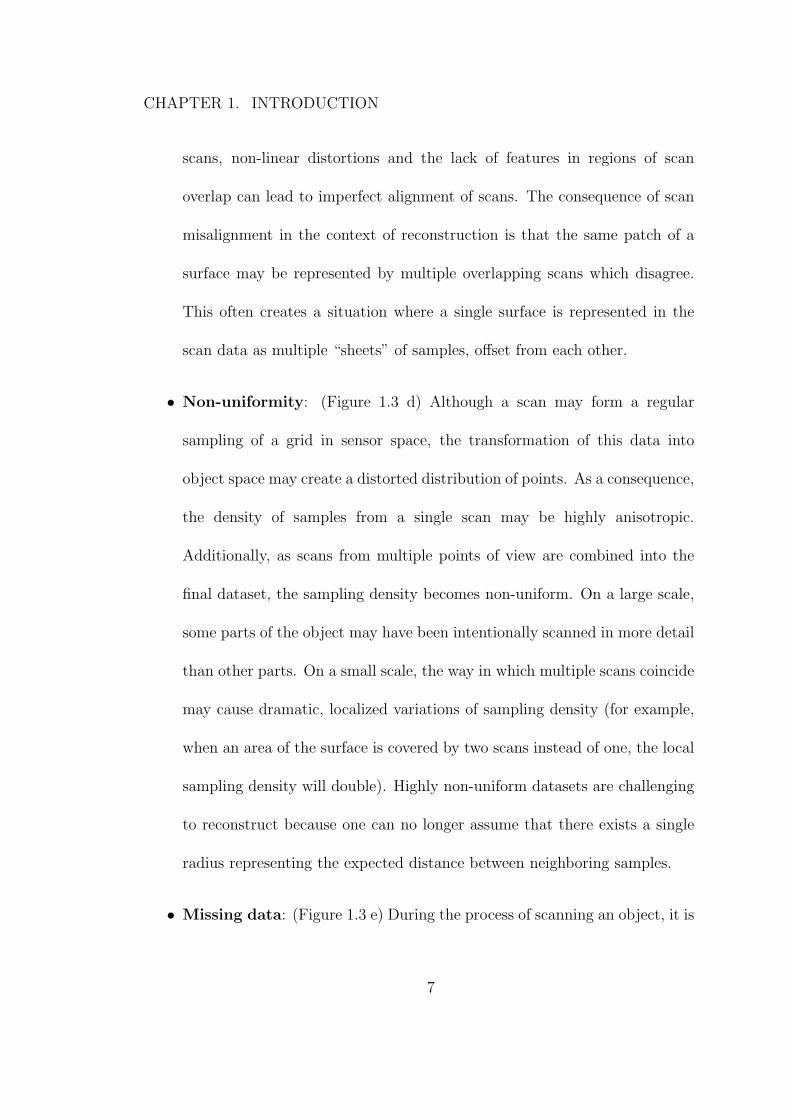
• Non-uniformity: (Figure 1.3 d) Although a scan may form a regular
sampling of a grid in sensor space, the transformation of this data into
object space may create a distorted distribution of points. As a consequence,
the density of samples from a single scan may be highly anisotropic.
Additionally, as scans from multiple points of view are combined into the
final dataset, the sampling density becomes non-uniform. On a large scale,
some parts of the object may have been intentionally scanned in more detail
than other parts. On a small scale, the way in which multiple scans coincide
may cause dramatic, localized variations of sampling density (for example,
when an area of the surface is covered by two scans instead of one, the local
sampling density will double). Highly non-uniform datasets are challenging
to reconstruct because one can no longer assume that there exists a single
radius representing the expected distance between neighboring samples.
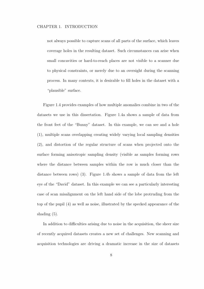
• Missing data: (Figure 1.3 e) During the process of scanning an object, it is
7
CHAPTER 1. INTRODUCTION
not always possible to capture scans of all parts of the surface, which leaves
coverage holes in the resulting dataset. Such circumstances can arise when
small concavities or hard-to-reach places are not visible to a scanner due
to physical constraints, or merely due to an oversight during the scanning
process. In many contexts, it is desirable to fill holes in the dataset with a
“plausible” surface.
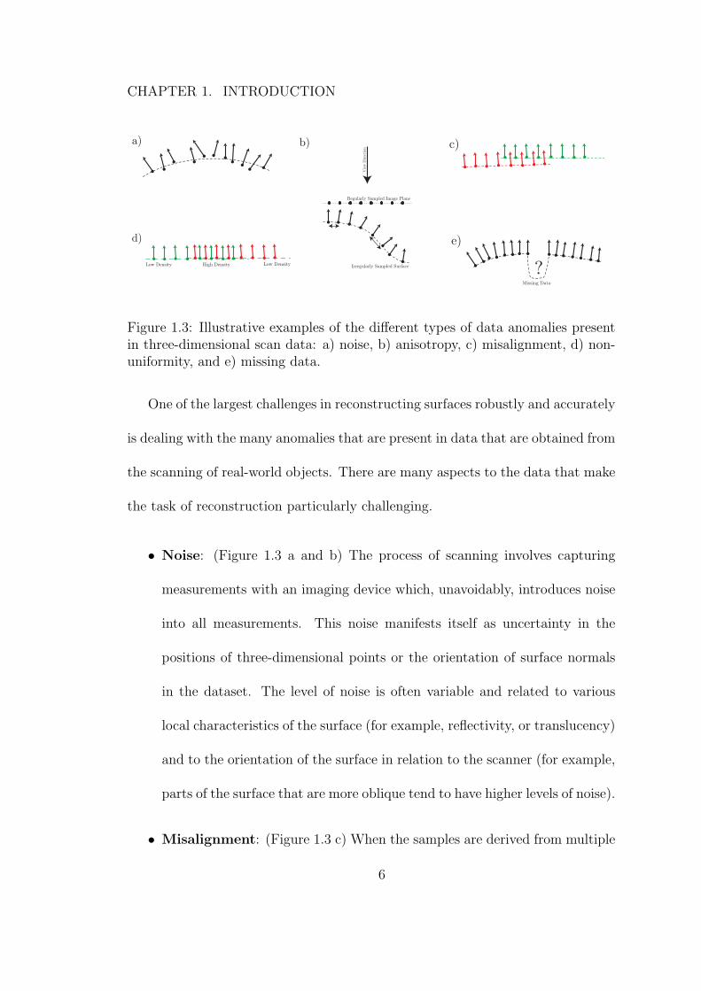
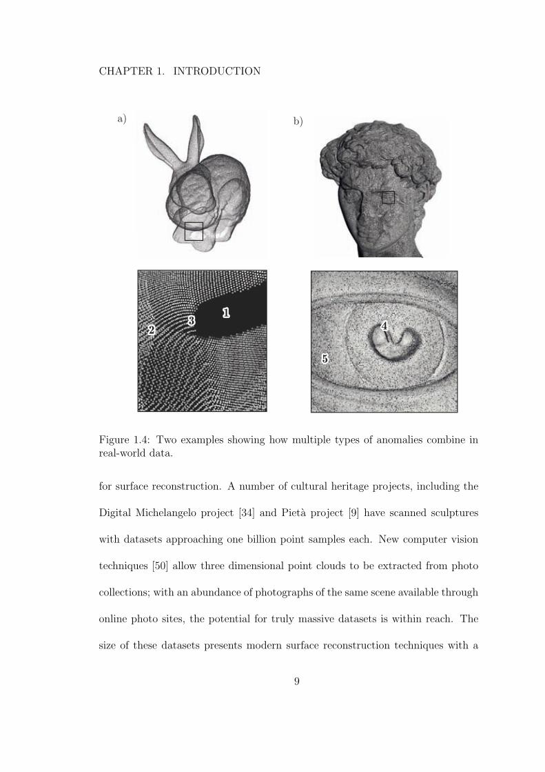
Figure 1.4 provides examples of how multiple anomalies combine in two of the
datasets we use in this dissertation. Figure 1.4a shows a sample of data from
the front feet of the “Bunny” dataset. In this example, we can see and a hole
(1), multiple scans overlapping creating widely varying local sampling densities
(2), and distortion of the regular structure of scans when projected onto the
surface forming anisotropic sampling density (visible as samples forming rows
where the distance between samples within the row is much closer than the
distance between rows) (3). Figure 1.4b shows a sample of data from the left
eye of the “David” dataset. In this example we can see a particularly interesting
case of scan misalignment on the left hand side of the lobe protruding from the
top of the pupil (4) as well as noise, illustrated by the specked appearance of the
shading (5).
In addition to difficulties arising due to noise in the acquisition, the sheer size
of recently acquired datasets creates a new set of challenges. New scanning and
acquisition technologies are driving a dramatic increase in the size of datasets
8
CHAPTER 1. INTRODUCTION
a) b)
Figure 1.4: Two examples showing how multiple types of anomalies combine inreal-world data.
for surface reconstruction. A number of cultural heritage projects, including the
Digital Michelangelo project [34] and Pieta project [9] have scanned sculptures
with datasets approaching one billion point samples each. New computer vision
techniques [50] allow three dimensional point clouds to be extracted from photo
collections; with an abundance of photographs of the same scene available through
online photo sites, the potential for truly massive datasets is within reach. The
size of these datasets presents modern surface reconstruction techniques with a
9
CHAPTER 1. INTRODUCTION
new set of challenges: Processing such large datasets can require thousands of
hours of computing time and hundreds of gigabytes of storage.
1.3 Outline of Dissertation
In Chapter 2, we review a wide range of existing surface reconstruction
techniques and develop a taxonomy to group methods based on their design and
implementation. In Chapter 3 we present the Poisson Surface Reconstruction
algorithm, a new technique for reconstructing surfaces that is computationally
efficient and robust. In Chapter 4 we show that, despite being a global problem,
the Poisson technique can be extended to a streaming computation model,
allowing for the reconstruction of the extremely large datasets available from
large scale 3D scanning projects by only requiring a small subset of the data
to be accessible in memory at any one time. In Chapter 5 we show how the
streaming technique can be adapted to process the octree data in parallel, allowing
faster processing of large datasets on both shared memory and distributed memory
computer systems. We conclude in Chapter 6 with a summary of our work, and
a brief discussion of directions for future scholarship.
10
Chapter 2
Surface Reconstruction
Surface reconstruction has been a well studied problem in computer graphics
and vision and a wide variety of methods have been suggested. The general
approach of a surface reconstruction method can be most broadly categorized
as either discrete or continuous. Discrete methods utilize the pointset directly,
or structures from computational geometry to define the surface. Continuous
methods take either a surface fitting approach, where a surface is fit directly to
the samples, or a function fitting approach, where an implicit function is first fit
to the samples and then used to define a surface.
There are a wide range of methods for scanning. In addition to triangulation
based range scanners, many techniques from computer vision, including shape
from stereo [7] and shape from shading [26] can take images of an object and
produce a three-dimensional representation. Because of this diversity, there are
11
CHAPTER 2. SURFACE RECONSTRUCTION
several different forms in which input data for surface reconstruction can take.
Many techniques make use of these different forms to aid the reconstruction
process. In the most general form, the surface is represented by a point set
P = {p1, ..., pN} where pi ∈ R3 are a sampling of positions on (or near) a surface.
In addition to position of each sample, many scanning techniques can also provide
information about the orientation of the surface at each sample point. In these
cases, the scan data data forms an oriented point set P = {(p1, n1), ..., (pN , nN)}
where pi, ni ∈ R3 and ni represents the normal vector at each sample. A more
specialized, but very common form of scan data, is the range image. A range image
is a two-dimensional regular grid R ∈ RN×M of values where each value represents
the distance from the scanner source to points on a surface. With information
such as the position of the scanner center and the scanner’s orientation, the three-
dimensional location of sample points can be computed from each element of
the range image. Additionally, the implicit array structure provides connectivity
between adjacent points, allowing the range image to represent a quadrangulated
patch of a surface. Using this topology, a range image can also define a per sample
surface normal.
In the remainder of this chapter, we will briefly describe some of the
more significant surface reconstruction methods from the literature following the
taxonomy of Figure 2.1. We also classify each method according to the type of
input data required in Figure 2.2.
12
CHAPTER 2. SURFACE RECONSTRUCTION
Surface Reconstruction
Continuous Discrete
Function FittingSurface Fitting Computational Geometry
Global Function Fitting Local Function Fitting
Co-cone
Signed Distance
Density Field
Local Function Fitting
Signed DistanceIndicator Function Voronoi
Computational Geometry
DelaunayBalloon Fitting
Point Set Surfaces
Ball Pivoting
Alpha Shapes
Power CrustFFT
VRIP
Blobby Models
Fast RBF
Hoppe et.al.
MPUWavelets
Poisson
Fast Level Set
Figure 2.1: A taxonomy of surface reconstruction methods, based on the generalapproach to solving the reconstruction problem.
Oriented Point SetPoint Set Range Images
Alpha Shapes
FFT
VRIP
Blobby Models
Fast RBF
Hoppe et.al.
MPU
Wavelets
PoissonCo-cone
Balloon Fitting
Point Set Surfaces
Ball Pivoting
Power Crust
Fast Level Set
Figure 2.2: A categorization of surface reconstruction methods, based on the typeof input data required.
13
CHAPTER 2. SURFACE RECONSTRUCTION
2.1 Discrete Methods
2.1.1 Computational Geometry
Many of the earliest approaches to surface reconstruction used techniques from
computational geometry. In general, these approaches take a set of points and
compute combinatorial structures such as the Delaunay teterahedralization or
Voronoi diagram. From these partitions of space, a labeling process defines each
partition as either interior or exterior to the shape, and the reconstructed surface
is defined as the set of faces between interior and exterior regions. The surface
that results from this process typically interpolate most or all of the points in P .
2.1.2 Alpha Shapes
Among the first of these was alpha shapes [20]. The alpha-shape Sα(P ) of a
point-set P is a simplical complex that can be thought of as a generalization of
the convex hull, parameterized by α. As α → ∞, the alpha shape is the convex
hull of P . As α→ 0, the alpha shape is P itself. For other values of alpha, a set
of shapes are defined which are constructed from the Delaunay tetrahedralization
DT (P ). The alpha shape is formed by iteratively removing all exposed edges of
DT (P ) where |xi − xj| < α, i 6= j. Faces and tetrahedra are removed from Sα
when one of their corresponding edges or faces is removed.
14
CHAPTER 2. SURFACE RECONSTRUCTION
Although simple to construct, alpha shapes have limited utility in surface
reconstruction, especially when reconstructing from real-world data. Because α is
a global parameter, it can be hard to choose a single α-value that can be used to
extract a good representation of the surface everywhere: this becomes increasingly
challenging when sampling density in P is non-uniform. Additionally, because
Sα(P ) is an arbitrary simplical complex, the resulting shape is not guaranteed to
be manifold.
2.1.3 Power Crust
The power crust algorithm [4, 5] reconstructs a surface S by making the
observation that a surface can be represented by it’s medial axis, or skeleton –
MAT (S). The medial axis is defined as the set of all points that are equi-distant
to two or more points on S. The power crust algorithm approximates MAT (S) by
constructing the Vornoni diagram of P , V (P ). From V (P ) the Voronoi Venice’s
that form poles are used to define the points on the medial axis and are used to
construct a set of polar balls. A vertex v ∈ V (P ) is a pole p if it is the farthest
vertex from the center of a Voronoi cell that it belongs to. Each pole defines
a ball centered at p with a radius equal to the distance of p from the nearest
point in P . To compute a surface, the polar balls are used to construct a power
diagram (a Voronoi diagram of the poles, weighted by radius), cells of the power
diagram are labelled as “interior” and the surface (“power crust”) is extracted as
15
CHAPTER 2. SURFACE RECONSTRUCTION
the boundary.
With the power crust algorithm, Amenta et al. also provided theoretical
guarantees. In particular, provided P is sufficiently dense, the surface that
the power crust algorithm reconstructs is a (provably) smooth surface that is
homeomorphic to the surface from which the points were sampled. Formally, a
set of samples is defined to be sufficiently dense when the distance from any surface
point to the nearest sample is at most a small constant ε times the distance to
medial axis. Intuitively, this means that P must be more densely sampled in
regions of high curvature, or regions where other parts of the surface are nearby.
2.1.4 Ball Pivoting
The ball pivoting algorithm [8] reconstructs a surface S from a point cloud
P using a ball of radius ρ. The surface is constructed from the set of triangles
constructed from three distinct points in P which can form a ball of radius ρ
without containing any other points from P . The algorithm is implemented by
taking a “seed” ball and successively pivoting the ball across triangle edges until
no more points can be visited. Although this method is highly efficient and can
operate on large datasets, it has a number of practical limitations. Like methods
from computational geometry, this method produces a surface that interpolates
most of the input points, which can reconstruct undesirable sampling noise. In
addition, as with alpha shapes, the value of ρ is constant which reduces the utility
16
CHAPTER 2. SURFACE RECONSTRUCTION
when dealing with non-uniform data.
2.2 Continuous Methods
2.2.1 Surface Fitting
Surface fitting approaches take a set of points and deforms a base shape until
it fits the points.
2.2.1.1 Balloon Fitting
The “Balloon Fitting” method of Chen et al. [15] uses an approach inspired by
the inflation of a balloon. The method takes a point set P as an input, along with
a seed surface S (an icosahedron) that is completely contained inside the desired
surface. S is used to form a mass-spring system where each vertex is connected
to its neighbors via springs. The surface is iteratively grown by increasing the
internal pressure of S, which causes each triangle to inflate in the direction of its
surface normal. To ensure that triangles in S are kept sufficiently small, triangles
are split when the spring force acting between two vertices exceeds some threshold.
Once a triangle in S reaches a point in P , or, has no points in P in front of it (i.e.
a hole) the vertices of the triangle become “anchored” and do not move in future
updates. The surface is complete once all vertices become anchored.
17
CHAPTER 2. SURFACE RECONSTRUCTION
In practice, there are two difficulties with the “Balloon Fitting” method. First,
finding a seed surface automatically is not an easy problem, typically requiring
user intervention. Second, because of the way the surface is inflated to fit the
model, the genus of the surface is restricted to be the genus of the seed surface.
2.2.1.2 Fast Level Set Method
The fast level set method of Zhao et al. [58] takes an implicit approach
to the surface-fitting problem. Given a general input data set (S) that may
contain points, curves or surface patches, a distance function d(x) = dist(x, S)
is computed. Given an arbitrary initial surface Γ, an energy function E(Γ) is
defined using d(x) and the energy flow is used to evolve the surface toward a
better approximation of S.
Because the topological structure of the reconstructed surface is not known
a priori, it is not effective to represent Γ in an explicit form. Instead, this
method uses a level set formulation, allowing the toplogy of the surface to change
throughout the evolution process.
2.2.1.3 Point Set Surfaces
The “Point Set Surfaces” method of Alexa et al. [3] uses the moving least
squares (MLS) projection operator [33] to define a surface M implicitly from a set
of points P . The MLS operator is a projection operator Π that takes a point r and
18
CHAPTER 2. SURFACE RECONSTRUCTION
maps it to the unknown surface S. Given a point r that is near M , the projection
operator is formed by fitting a plane H around r that minimizes the weighted
sum of squared distances to all pi ∈ P . Using the plane H as a parametrization
domain, the surface is locally represented by the graph of a polynomial function
g with approximates the heights of the pi over H. The projection operator is
then defined by projecting r onto H and evaluating g at the projected point to
obtain the height of Π(r) over H. One aspect of this method that is different
to all other methods we discuss in this chapter, is that the reconstructed surface
S is not represented as a mesh, but as a dense collection of points that can be
rendered with point-based rendering methods [35].
2.2.2 Implicit Function Fitting
Function fitting approaches attempt to define a function F : R3 → R such
that the interior and exterior of the shape can be distinguished and the surface
can be extracted as a level-set of F . In its essence, surface reconstruction via
implicit function fitting is a scattered data interpolation problem [21]: The input
point set forms a set of constraints to which an unknown function F is fit. A
variety of different choices for F have been used, including signed [13, 17,25] and
unsigned [42] distance functions, and the indicator function [31,39].
19
CHAPTER 2. SURFACE RECONSTRUCTION
2.2.3 Local Function Fitting
In contrast to global function fitting approaches in which an input sample
can influence the values of F over the entire domain, in local function fitting
approaches a sample only influences the values of F in a small, localized
neighborhoods. In practice, these approaches tend to be efficient because the
local reconstruction of the surface only needs to consider a small subset of points
from the dataset. The challenge for local methods is defining the locality of a
sample. If the choice of neighborhood is too small, errors in the data, such as
noise and misalignment can result in undesirable artifacts in the resulting surface.
When the neighborhood is large, the solution can become inefficient to compute.
2.2.3.1 Hoppe et al.
The approach of Hoppe et al. [25] was one of the first function fitting
approaches to reconstruct a surface from an unorganized point set (i.e. a set
of three-dimensional points with no normal or topological information). This
approach constructs an approximation to the signed distance function, F , of the
unknown surface. The signed distance function of a surface S, is a scalar function
F : R3 → R where the value of F (x) is defined as the Euclidean distance of x
from the nearest point on S with points inside S assigned a negative distance,
and points outside assigned a positive distance value. Once F is computed, the
surface is extracted as the zero-set of F using a contouring algorithm.
20
CHAPTER 2. SURFACE RECONSTRUCTION
To define F , each point pi ∈ P is associated with an oriented plane Ti ≡
〈pi, ni〉 = 0 which defines a local linear approximation to the Euclidean distance
function of the surface. Each Ti is estimated by fitting a plane to the k-nearest
points to pi in P . The plane normal is defined as the smallest eigen-vector of the
covariance matrix of the points in the neighborhood.
To define surface normals that are consistently oriented (essential to robustly
construct the signed distance function) an additional step is taken to correctly
orient the tangent planes. To do this, a graph is formed where each tangent plane
Ti forms a node Ni in the graph. Two nodes of the graph Ni and Nj are connected
with an edge when the k-neighborhoods of Ti and Tj have at least one point in
common. Edges are weighted according to the absolute value of the dot product
of ni and nj. Then, a minimal spanning tree of the graph is created and the
normal directions are defined by assigning an (arbitrary) orientation to a node
and propagating the orientation through the tree.
2.2.3.2 Volumetric Range Image Processing (VRIP)
The Volumetric Range Image Processing (VRIP) method [17] reconstructs
surfaces from an aligned set of range images. From each range image Ri, a view
dependent signed distance function di(x) and a corresponding weight function
wi(x) are constructed. Then, a combined distance function D(x) is constructed
asP
wi(x)dj(x)Pwi(x)
and a surface is extracted as the iso-surface D−1(0).
21
CHAPTER 2. SURFACE RECONSTRUCTION
To prevent the distance function di of one scan influencing D far away from the
scan, the weight function wi tapers to zero over a small distance called the ramp
size. The ramp size is typically chosen to be half the maximum error expected in
range image distances. Because of the spatial locality of wi, large portions of widi
(and therefore D) are zero. This is exploited to reduce the storage requirements
of D by using run-length encoding.
In general, regions of the surface without range image coverage will not have a
well-defined iso-surface, leaving boundary contours in the reconstructed surface.
To seal some of these holes, VRIP uses space carving to exploit the fact that a range
image not only gives information about where the surface is, but also where it is
not. This is used to label the parts of space at which the view from the scanner is
un-occluded. Carving out the un-occluded regions from the reconstruction volume
results in an effective way for sealing some of these holes.
2.2.3.3 Multi-level Partitions of Unity (MPU)
The MPU [43] method reconstructs an approximation to the signed distance
function from an oriented point set. The signed distance function F is defined as
a set of locally defined functions fi blended together with a set of weights which
form a partition of unity (that is, for a given point x the weights always sum to
one). To construct the local functions fi an octree is used to recursively partition
space. For a given octree node oi, a (piecewise) quadratic approximation Qi is
22
CHAPTER 2. SURFACE RECONSTRUCTION
fit to the samples that fall within the spatial bounds of the octree node. If Qi
is a poor representation of the points (as measured by the Taubin distance [51])
the octree node is split, and the fitting process is repeated for each octant. If
the number of points in an octree node is too small, Qi may not be a robust
representation. In these cases, the next closest points are incrementally included
in computing Qi until a minimum number of points is reached. Once a Qi has
been fit to all nodes in the octree, local signed distance functions fi are computed
from Qi. To form the final implicit function F , the fi are blended together using
the partition of unity.
2.2.4 Global Function Fitting
Global function fitting approaches consider all points when defining the value of
the implicit function at a location. In general, global approaches are more robust,
as a local effects like noise or scan misalignment have a less direct influence on
the value of the function. There have been a number of surface reconstruction
techniques that use global function fitting methods. We briefly describe some of
these approaches.
2.2.4.1 Blobby Models
The concept of the “Blobby Model” was introduced by Blinn [10]. The idea
was that a 3D model can be represented as an iso-surface of a field generated
23
CHAPTER 2. SURFACE RECONSTRUCTION
from a number of primitives: F (x) =∑N
i=1 bie−aifi(x) where bi and ai control the
amplitude and fall-off of the primitive and fi is a function that describes the shape
of the primitive (Often, fi(x) = ‖x−xi‖2, where xi is the origin of the primitive).
The work of Muraki [42] applied Blinn’s work to the context of surface
reconstruction. The problem is, given a range image R, to find a set of primitives
that can generate a blobby model representation of R. Since directly finding N
primitives to fit R is a difficult problem, a greedy approach is used. Starting with
N = 1, primitives are recursively split and an energy minimization problem is
solved to fit the new primitives.
One of the problems with using a blobby model approach for surface
reconstruction is a limitation of the blobby representation itself. First, because
the primitives are smooth functions, objects with sharp features require a large
number of primitives to be represented accurately. Second, because primitives
have global support, local changes may introduce undesirable artifacts in other
regions of F .
2.2.4.2 Fast RBF
The FastRBF approach [13] takes a scattered data interpolation interpretation
of the reconstruction problem. The authors define F to be an approximation to
the signed distance function of the surface. To define F , first, each sample point
pi is used to set a constraint on F such that F (pi) = 0. To avoid the trivial
24
CHAPTER 2. SURFACE RECONSTRUCTION
solution of F = 0, additional constraints are added. “Off surface” points pini and
pouti are defined as pi± δni that form constraints on F such that F (pin
i ) = −δ and
F (pouti ) = +δ. Care is taken to ensure that these interior and exterior constraints
do not conflict in regions where the surface folds together. To solve for F , a radial
basis function scheme is used. F is represented as the weighed sum of radial
basis function F (x) =∑N
i=1 wi φ(‖x − ci‖) where ci is a constraint center, wi is
a weight and φ(x) is a function that has global support. Given the values fi at
the constraint points, a set of weights wi can be found by solving a linear least
squares problem.
Because φ(x) has global support, the linear system to find wi is dense and
poorly conditioned, and is therefore difficult to solve robustly as N grows. To
use radial basis functions to reconstruct surfaces from a large number of points,
a number of optimizations and approximations are used. First, fast multi-pole
methods are used to evaluate F (x). This optimization works by reducing the
number of constraints that need to be evaluated at x by approximating clusters
of centers far from x as a single constraint. Second, a greedy algorithm is used
to iteratively fit a small number of constraints to a given point set in order to
reconstruct the surface to within a desired fitting accuracy.
25
CHAPTER 2. SURFACE RECONSTRUCTION
2.2.4.3 Fast Fourier Transform
The work of Kazhdan [31] was the first function fitting method which used
the indicator function as its choice of implicit function. For a given solid M , the
indicator function χM is a scalar function that is defined as χM(x) = 1 if x ∈ M
and χM(x) = 0 otherwise. The FFT method constructs the indicator function
through an application of Stokes’ theorem, which expresses a volume integral as
a surface integral, a quantity that can be approximated from an oriented point
set. Specifically, the work shows that the Fourier coefficients of the indicator
function can be expressed as surface integrals computed using the oriented point
samples. As a result, the indicator function can be obtained by computing the
Fourier coefficients and running the inverse Fourier transform. The surface is
then extracted from the volume using the marching cubes [37] algorithm. Non-
uniformity in the input point set is handled by weighting the contribution of each
oriented point to the vector field by the result of a kernel density estimator.
Because of its global nature, the FFT method is robust to a variety of
degeneracies in the input data, including noise (in both sample position, and
orientation) and non-uniform sampling. Holes in the input data are plausibly
and smoothly filled in the output mesh. However, a significant disadvantage of
this method is the spatial and temporal complexity. Using an O(r3) regular grid
limits the practicality of the method when reconstructing large models with high
resolution. More recent work by Schall et al. [46] has taken the FFT approach and
26
CHAPTER 2. SURFACE RECONSTRUCTION
used it in an adaptive setting. This approach partitions a large model using an
adaptive octree and computes a number of local FFT’s that get blended for the
final indicator function, in a manner similar to the blending of the MPU approach.
Although this provides a more scalable solution than the original method, the local
decisions used to form and blend local FFT reconstructions can make the method
less robust.
2.2.4.4 Wavelets
The Wavelet based-approach of Manson et al. [39] uses a similar approach as
the FFT method, computing the indicator function from an oriented point set
using Stokes’ theorem. However, instead of using the Fourier basis, this method
uses an orthogonal wavelet basis with compact support. The key observation is
that, in the case of the Fourier basis, computing each Fourier coefficient requires
summation across all of sample points. In contrast, when using a wavelet basis
(with compactly supported basis functions) computing each wavelet coefficient
only requires the summation of samples within the support of the basis.
This approach offers a number of practical advantages over the FFT based
method. First, the algorithm is more efficient. Second, the spatial complexity of
the algorithm is lower, since only wavelet coefficients whose support overlaps the
sample points need to be stored explicitly.
27

CHAPTER 2. SURFACE RECONSTRUCTION
2.2.4.5 Our Approach
The approach that we describe in this dissertation is similar in spirit to
the FFT approach. Like the FFT approach, we reconstruct surfaces by first
constructing an approximation the indicator function χ from a set of oriented
points, and then extracting a surface from χ. We address a number of the
limitations of the FFT approach by using an adaptive function basis formed on
in octree.
28

Chapter 3
Poisson Surface Reconstruction
Reconstructing 3D surfaces from point samples is a well-studied problem in
computer graphics. It allows for the fitting of surfaces to scanned data, the filling
of surface holes, and the re-meshing of existing models. In this chapter, we describe
a surface reconstruction approach that expresses surface reconstruction as the
solution to a Poisson equation.
3.1 The Poisson Idea
Like much previous work, we approach the problem of surface reconstruction
using an implicit function framework. Specifically, like [31] we compute a 3D
indicator function χ (defined as 1 at points inside the model, and as 0 at points
outside), and then obtain the reconstructed surface by extracting an appropriate
29
CHAPTER 3. POISSON SURFACE RECONSTRUCTION
1
1
1
0
0
M
0
0
00 0
1
1
1
0
Indicator function
M
Indicator gradient
0 0
0
0
0
0
Surface
MOriented points
V
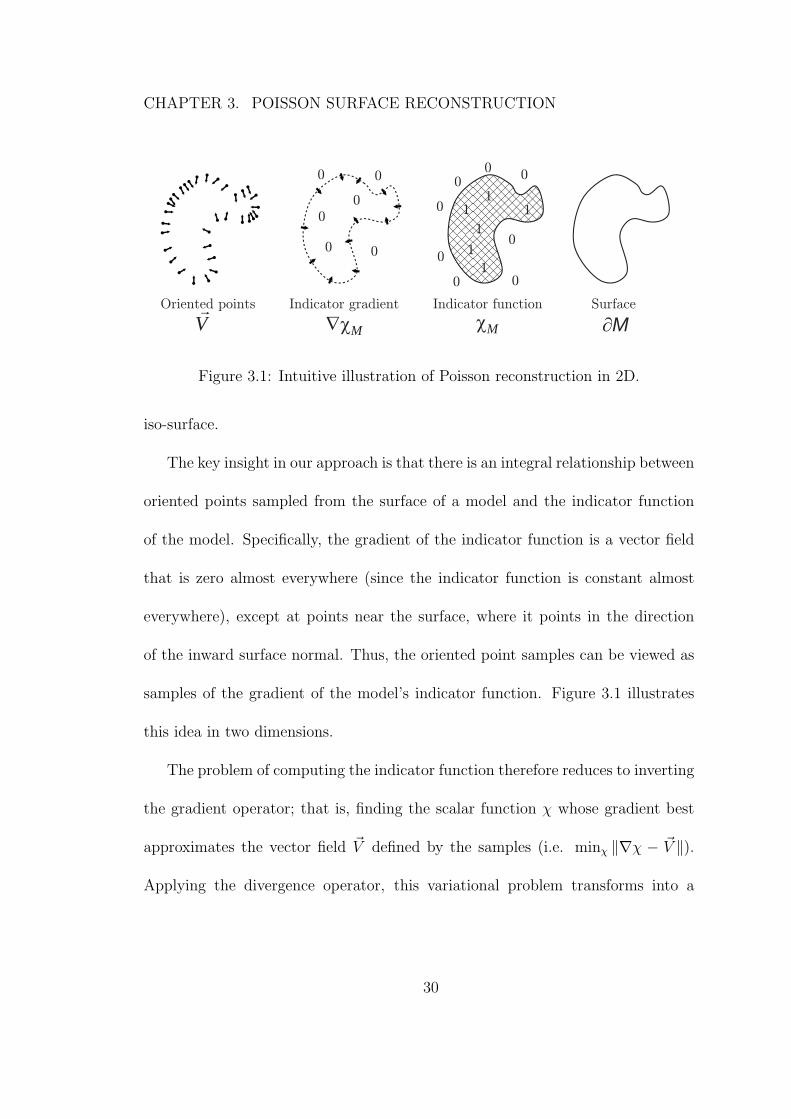
Figure 3.1: Intuitive illustration of Poisson reconstruction in 2D.
iso-surface.
The key insight in our approach is that there is an integral relationship between
oriented points sampled from the surface of a model and the indicator function
of the model. Specifically, the gradient of the indicator function is a vector field
that is zero almost everywhere (since the indicator function is constant almost
everywhere), except at points near the surface, where it points in the direction
of the inward surface normal. Thus, the oriented point samples can be viewed as
samples of the gradient of the model’s indicator function. Figure 3.1 illustrates
this idea in two dimensions.
The problem of computing the indicator function therefore reduces to inverting
the gradient operator; that is, finding the scalar function χ whose gradient best
approximates the vector field ~V defined by the samples (i.e. minχ ‖∇χ − ~V ‖).
Applying the divergence operator, this variational problem transforms into a
30
CHAPTER 3. POISSON SURFACE RECONSTRUCTION
standard Poisson problem:
∆χ ≡ ∇ · ∇χ = ∇ · ~V . (3.1)
We will make these definitions precise in Sections 3.2 and 3.3.
Formulating surface reconstruction as a Poisson problem offers a number of
advantages. Many implicit surface fitting methods first segment the data into
regions for local fitting, and then combine these local approximations using
blending functions. In contrast, Poisson reconstruction is a global solution
that considers all the data at once, without resorting to heuristic partitioning
or blending. Thus, like radial basis function (RBF) approaches, Poisson
reconstruction creates smooth surfaces that robustly fit noisy data. But, whereas
ideal RBFs are globally supported and non-decaying, the Poisson problem admits
a hierarchy of locally supported functions, and therefore its solution reduces to a
well-conditioned sparse linear system.
Moreover, in many implicit fitting schemes, the value of the implicit function
is constrained only near the sample points, and consequently the reconstruction
may contain spurious surface sheets away from these samples. Typically, this
problem is reduced by introducing auxiliary “off-surface” points (e.g. [13, 43]).
With Poisson surface reconstruction, such surface sheets do not arise because the
gradient of the implicit function is constrained at all spatial points. In particular,
it is constrained to zero away from the samples.
31
CHAPTER 3. POISSON SURFACE RECONSTRUCTION
There has been broad interdisciplinary research on solving Poisson problems
and many efficient and robust methods have been developed. One particular
aspect of our problem instance is that an accurate solution to the Poisson equation
is only necessary near the reconstructed surface. This allows us to leverage
adaptive Poisson solvers to develop a reconstruction algorithm whose spatial and
temporal complexities are proportional to the size of the reconstructed surface.
3.2 Approach
The input to the surface reconstruction is an oriented point set P = {si =
(p1, n1), ..., sN = (pN , nN)} that consists of a sample si with a position s.p and an
inward-facing normal s.n, assumed to lie on or near the surface ∂M of an unknown
model M . The goal is to reconstruct a watertight, triangulated approximation to
the surface by approximating the indicator function of the model and extracting
the iso-surface, as illustrated in Figure 3.2.
In the next sections, we derive a relationship between the (smoothed) gradient
of the indicator function and an integral of the normal field over the surface. We
then approximate this surface integral by a summation over the given oriented
point samples. Finally, we reconstruct the indicator function from this gradient
field as the solution to a Poisson problem.
32
CHAPTER 3. POISSON SURFACE RECONSTRUCTION
3.2.1 Defining the gradient field
Because the indicator function is a piecewise constant function, explicit
computation of its gradient field would result in a vector field with unbounded
values at the surface boundary. To avoid this, we convolve the indicator function
with a smoothing filter and consider the gradient field of the smoothed function.
The following lemma formalizes the relationship between the gradient of the
smoothed indicator function and the surface normal field.
Lemma: Given a solid M with boundary ∂M , let χM denote the indicator
function of M , ~N∂M(p) be the inward surface normal at p ∈ ∂M , F (q) be a
smoothing filter, and Fp(q) = F (q−p) its translation to the point p. The gradient of
the smoothed indicator function is equal to the vector field obtained by smoothing
the surface normal field:
∇(χM ∗ F
)(q0) =
∫∂M
Fp(q0) ~N∂M(p)dp. (3.2)
Proof: To prove this, we show equality for each of the components of the vector
field. Computing the partial derivative of the smoothed indicator function with
33
CHAPTER 3. POISSON SURFACE RECONSTRUCTION
respect to x, we get:
∂
∂qx
∣∣∣∣q0
(χM ∗ F
)(q) =
∂
∂qx
∣∣∣∣q0
∫M
F (q − p)dp
=
∫M
(− ∂
∂px
F (q0 − p)
)dp
= −∫
M
∇ ·(F (q0 − p), 0, 0
)dp
=
∫∂M
⟨(Fp(q0), 0, 0
), ~N∂M(p)
⟩dp.
(The first equality follows from the fact that χM is equal to zero outside of
M and one inside. The second follows from the fact that (∂/∂qx)F (q − p) =
−(∂/∂px)F (q − p). The last follows from the Divergence Theorem.)
A similar argument shows that the y, and z-components of the two sides are
equal, thereby completing the proof. �
3.2.2 Approximating the gradient field
Of course, we cannot evaluate the surface integral since we do not yet know
the surface geometry. However, the input set of oriented points provides precisely
enough information to approximate the integral with a discrete summation.
Specifically, using the point set P to partition ∂M into distinct patches Ps ⊂ ∂M ,
we can approximate the integral over a patch Ps by the value at point sample s.p,
34
CHAPTER 3. POISSON SURFACE RECONSTRUCTION
scaled by the area of the patch:
∇(χM ∗ F )(q) =∑s∈P
∫Ps
Fp(q) ~N∂M(p)dp
≈∑s∈P
|Ps| Fs.p(q) s.n ≡ ~V (q).
(3.3)
It should be noted that although Equation 3.2 is true for any smoothing filter
F , in practice, care must be taken in choosing the filter. In particular, we would
like the filter to satisfy two conditions: (1) it should be sufficiently narrow so that
we do not over-smooth the data; (2) it should be wide enough so that the integral
over Ps is well approximated by the value at s.p scaled by the patch area. A good
choice of filter that balances these two requirements is a Gaussian whose variance
is on the order of the sampling resolution.
3.2.3 Solving the Poisson problem
Having formed a vector field ~V , we want to solve for the function χ such that
∇χ = ~V . However, ~V is generally not integrable (i.e. it is not curl-free), so an
exact solution does not generally exist. To find the least-squares solution, we
apply the divergence operator to form the Poisson equation:
∆χ = ∇ · ~V (3.4)
35
CHAPTER 3. POISSON SURFACE RECONSTRUCTION
Figure 3.2: Points from scans of the “Armadillo Man” model (left), our Poissonsurface reconstruction (right), and a visualization of the indicator function(middle) along a plane through the 3D volume.
3.3 Implementation
In this section, we describe our implementation of the Poisson surface
reconstruction algorithm in more detail. We first present our algorithm under
the assumption that the point samples are uniformly distributed over the model
surface. We define a space of functions with high resolution near the surface of
the model and coarser resolution away from it; we express the vector field ~V as
a linear sum of functions in this space; we set up and solve the Poisson equation;
and we extract an iso-surface of the resulting indicator function. The extension
of the algorithm to the case of non-uniformly sampled points is described in the
next section.
36
CHAPTER 3. POISSON SURFACE RECONSTRUCTION
3.3.1 Problem Discretization
First, we must choose the space of functions over which to discretize the
problem. The most straightforward approach is to start with a regular 3D
grid [31]. However, such a uniform structure becomes impractical for fine-detail
reconstruction, since the dimension of the space is cubic in the resolution while
the number of surface triangles grows quadratically.
Fortunately, an accurate representation of the implicit function is only
necessary near the reconstructed surface. This motivates the use of an adaptive
octree, both to represent the implicit function and to solve the Poisson system
(e.g. [23, 38]). Specifically, we use the positions of the sample points to define an
octree O and associate a function Fo to each node o ∈ O of the tree, choosing the
tree and the functions so that the following conditions are satisfied:
1. The vector field ~V can be precisely and efficiently represented as the linear
sum of the Fo;
2. The matrix representation of the Poisson equation, expressed in terms of
the Fo, can be solved efficiently; and
3. A representation of the indicator function as the sum of the Fo can be
precisely and efficiently evaluated near the surface of the model.
37
CHAPTER 3. POISSON SURFACE RECONSTRUCTION
3.3.1.1 Defining the function space
Given a set of point samples P and a maximum tree depth D, we define the
octree O to be the minimal octree with the property that every point sample falls
into a leaf node at depth D. Next, we define a space of functions obtained as the
span of translates and scales of a fixed base function F : R3 → R. For every node
o ∈ O, we set Fo to be the “node basis function” centered about the node o and
stretched by the size of o:
Fo(q) ≡ F
(q − o.c
o.w
)(3.5)
where o.c and o.w are the center and width of node o.
This space of functions FO,F ≡ Span{Fo} has a multi-resolution structure:
functions associated with finer nodes encode higher frequencies, and the function
representation becomes more precise as we near the surface. Note that, because
the space is adaptive, not all coarse functions can be represented as a linear
combination of finer functions. Thus, the functions we will consider will be
represented as linear combinations of nodal basis functions across all levels, not
just the basis functions at the finest level.
38
CHAPTER 3. POISSON SURFACE RECONSTRUCTION
3.3.1.2 Selecting a base function
In selecting a base function F , our goal is to choose a function so that the vector
field ~V , defined in Equation 3.3, can be precisely and efficiently represented as the
linear sum of the node functions {Fo}.
Since a maximum tree depth of D corresponds to a sampling width of 2−D,
the smoothing filter should approximate a Gaussian with variance on the order of
2−D. Thus, F should approximate a Gaussian with unit-variance.
For efficiency, we approximate the unit-variance Gaussian by a compactly
supported function so that: (1) the resulting Divergence and Laplacian operators
are sparse; and (2) the evaluation of a function expressed as the linear sum of Fo
at some point q only requires summing over the nodes o ∈ O that are close to q.
Thus, we set F to be the n-th convolution of a box filter with itself resulting in
the base function F :
F (x, y, z) ≡ (B(x)B(y)B(z))∗n with B(t) =
1 |t| < 0.5
0 otherwise
(3.6)
Note that as n is increased, F more closely approximates a Gaussian and
its support grows larger: in our implementation we use a piecewise quadratic
approximation with n = 3. Therefore, the function F is supported on the domain
[−1.5, 1.5]3 and, for the basis function of any octree node, there are at most
53 − 1 = 124 other nodes at the same depth whose functions have overlapping
39
CHAPTER 3. POISSON SURFACE RECONSTRUCTION
support.
3.3.2 Vector Field Definition
If we were to replace the position of each sample with the center of the leaf node
in which it falls, the vector field ~V could be simply expressed as the linear sum of
{Fo}. This way, each sample would contribute a single term (the normal vector)
to the coefficient corresponding to its leaf’s node function. Since the sampling
width is 2−D and the samples all fall into leaf nodes of depth D, the error arising
from the clamping can never be too big (at most, on the order of half the sampling
width). To allow for sub-node precision, we avoid clamping a sample’s position to
the center of the containing leaf node and instead use interpolation to distribute
the sample across the one ring neighborhood of nodes. In particular, we define
our approximation to the gradient field of the indicator function as:
~V (q) =∑
o∈OD
Fo(q)vo (3.7)
with
vo =∑s∈P
Fo(s.p)s.n (3.8)
where OD is the set of all nodes from the octree at depth D. Note that Fo(s.p)
is only non-zero when o is in the one-ring neighborhood of the node containing
s.p. Thus, in practice, the coefficients of the vector field can be computed by
40
CHAPTER 3. POISSON SURFACE RECONSTRUCTION
“splatting” the normal vector s.n into the one-ring neighborhood of s.p. To ensure
that we have an adequate ability to represent ~V in this way, we construct the
octree so that a node o is in the tree whenever there exists an s ∈ P such that
Fo(s.p) 6= 0.
Since we assume that the samples are uniform, the area of a patch Ps is
constant and ~V is a good approximation, up to a multiplicative constant, of the
gradient of the smoothed indicator function. We will show that the choice of
multiplicative constant does not affect the reconstruction.
3.3.3 Linear System Definition
Having defined the vector field ~V , we would like to solve for the function
χ ∈ FO,F whose gradient is closest to ~V : that is, we would like to solve the
Poisson equation ∆χ = ∇ · ~V . One challenge of solving for χ is that although
χ and the coordinate functions of ~V are in the space FO,F , it is not necessarily
the case that the functions ∆χ and ∇ · ~V are. To address this issue, we need to
solve for the function χ such that the projection of ∆χ onto the space FO,F is
equals the projection of ∇ · ~V . Since, in general, the functions Fo do not form an
orthonormal basis, solving this problem directly is expensive. However, we can
simplify the problem using the Galerkin formulation by solving for the function χ
41
CHAPTER 3. POISSON SURFACE RECONSTRUCTION
with:
〈∆χ, Fo〉 = 〈∇ · ~V , F0〉 (3.9)
for all o ∈ O. Thus given the |O|-dimensional vector b whose o-th coordinate
is bo = 〈∇ · ~V , Fo〉, the goal is to solve for the function χ such that the vector
obtained by taking the dot product of the Laplacian of χ with each of the Fo is
equal to b.
To express this in matrix form, we let χ =∑
o xoFo, so that we are solving for
the vector x ∈ R|O|. Then, we define the |O| × |O| matrix L so that Lx returns
the dot product of the Laplacian with each of the Fo. Specifically, for all o, o′ ∈ O,
the (o, o′)-th entry of L is set to:
Lo,o′ ≡⟨
∂2Fo
∂x2, Fo′
⟩+
⟨∂2Fo
∂y2, Fo′
⟩+
⟨∂2Fo
∂z2, Fo′
⟩. (3.10)
Thus, solving for χ amounts to finding
Lx = b (3.11)
Note that in solving for χ, we do not explicitly compute the projection of the
divergence of ~V onto FO,F . We only compute the dot product of the divergence
with each Fo. Since the Fo are compactly supported, this can be done efficiently.
42
CHAPTER 3. POISSON SURFACE RECONSTRUCTION
Note also that the matrix L is sparse and symmetric. (Sparse because the Fo are
compactly supported, and symmetric because∫
f ′′g = −∫
f ′g′.)
Furthermore, there is an inherent multiresolution structure on FO,F , so we use
a multigrid approach. The linear system Lx = b is transformed into successive
linear systems Ldxd = bd (solved using conjugate gradients), one per octree
depth d. The solutions at finer depths only consider the residual divergence not
accounted for at coarser depths. More precisely, after solving at depths d′ < d,
the divergence constraints are updated at depth d to subtract those components
of the constraints that have already been satisfied at the coarser resolutions:
bdo ← bd
o −∑d′<d
∑o′∈Od′
Lo,o′xo′ , (3.12)
where Od denotes the set of octree nodes at depth d. Note that this approach
means that we use a cascadic multigrid solver (i.e. we do no restrict finer solutions
back to coarser solutions).
3.3.4 Iso-Surface Extraction
In order to obtain a reconstructed surface ∂M , it is necessary first to select
an iso-value and then to extract the corresponding iso-surface from the computed
indicator function.
We choose the iso-value so that the extracted surface closely approximates the
43
CHAPTER 3. POISSON SURFACE RECONSTRUCTION
positions of the input samples. We do this by evaluating χ at the sample positions,
and use the average of the values for iso-surface extraction:
∂M ≡ {q ∈ R3∣∣ χ(q) = γ} with γ =
1
|S|∑s∈P
χ(s.p). (3.13)
This choice of iso-value has the property that scaling χ does not change the iso-
surface. Thus, knowing the vector field ~V up to a multiplicative constant provides
sufficient information for reconstructing the surface.
To extract the iso-surface from the indicator function, we use the method of [32]
which is similar to previous adaptations of the Marching Cubes [37] to an octree
representation (e.g. [47, 54, 55]), but supports non-conforming trees, preventing
cracks from arising when coarser nodes share a face with finer ones.
3.3.5 Non-uniform Samples
We now describe the extension of our method to the case of non-uniformly
distributed point samples. As in [31], our approach is to estimate the local
sampling density, and scale the contribution of each point accordingly. However,
rather than simply scaling the magnitude of a fixed -width kernel associated with
each point, we additionally adapt the kernel width. This results in a reconstruction
that maintains sharp features in areas of dense sampling and provides a smooth
fit in sparsely sampled regions. Figure 3.3 illustrates the problems associated with
44
CHAPTER 3. POISSON SURFACE RECONSTRUCTION
using a fixed-width kernel to perform sample density estimation. In (b) and (c), we
can see the reconstructions of the cow using a low and high resolutions (i.e. wider
and narrower kernels) respectively. Because of the highly non-uniform nature of
the input point set, the use of a fixed-width kernel cannot simultaneously produce
a good estimation of sample density in all regions, and one must choose between
accurately capturing sharp features (such as the head) or smoothly reconstructing
the sparsely sampled body. In contrast, the use of adaptive width density kernels,
illustrated in (d), allows both regions to be reconstructed accurately by adapting
the filter width to the sampling density.
3.3.5.1 Estimating local sampling density
Following the approach of [31], we implement the density computation using a
kernel density estimator [45]. The approach is to estimate the number of points in
a neighborhood of a sample by “splatting” the samples into a 3D grid, convolving
the “splatting” function with a smoothing filter, and evaluating the convolution
at each of the sample points.
We implement the convolution in a manner similar to Equation 3.7. For each
depth D ≤ D we compute a density estimator as the sum of node functions at
depth D:
WD(q) =∑
o∈OD
Fo(q)ko (3.14)
45
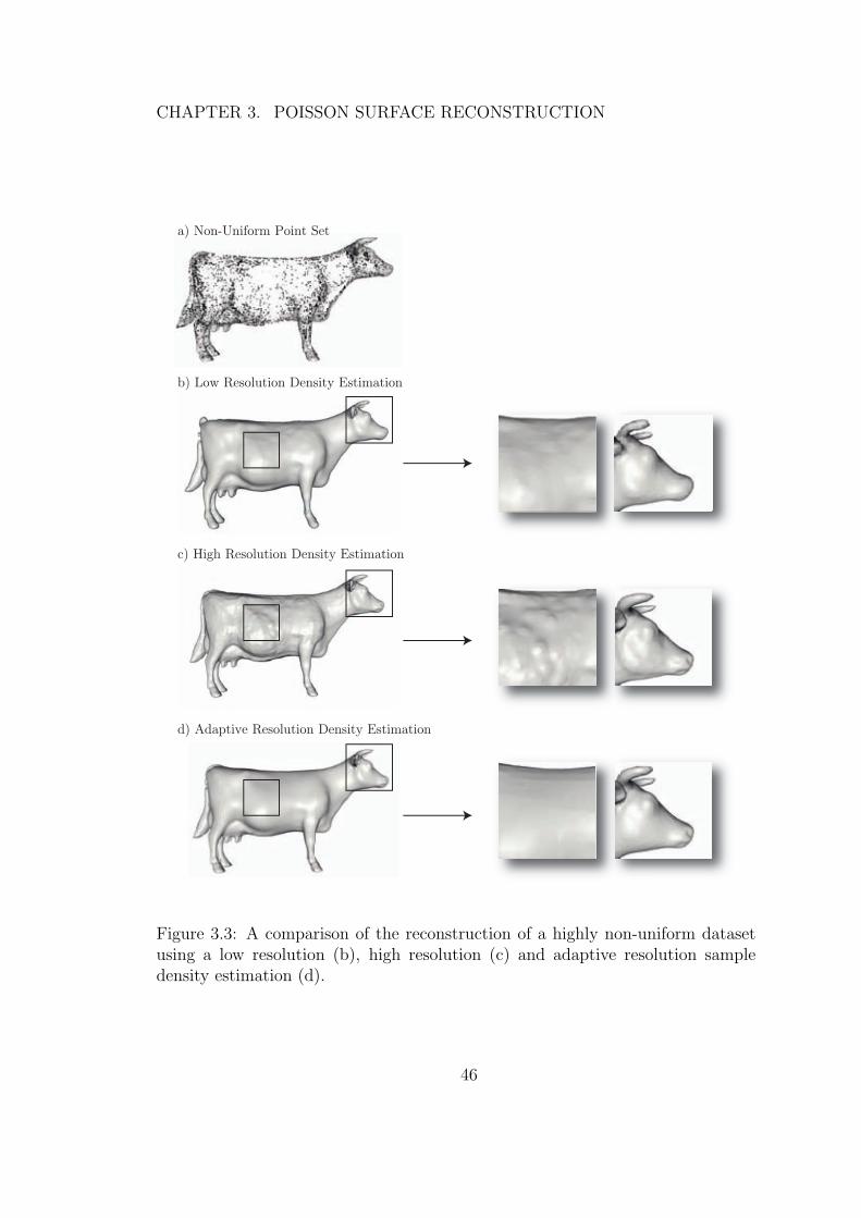
CHAPTER 3. POISSON SURFACE RECONSTRUCTION
a) Non-Uniform Point Set
b) Low Resolution Density Estimation
c) High Resolution Density Estimation
d) Adaptive Resolution Density Estimation
Figure 3.3: A comparison of the reconstruction of a highly non-uniform datasetusing a low resolution (b), high resolution (c) and adaptive resolution sampledensity estimation (d).
46
CHAPTER 3. POISSON SURFACE RECONSTRUCTION
with
ko =∑s∈P
Fo(s.p) (3.15)
Since octree nodes at lower resolution are associated with functions that
approximate Gaussians of larger width, computing WD at each level in the
tree provides a way to estimate sampling density over a wide range of widths.
Furthermore, because the basis functions at depth D form a partition of unity,
the weight WD(q) can be viewed as a (local) measure of the number of samples
falling into a node at depth D.
3.3.5.2 Estimating a samples depth
Given a user-supplied parameter κ, which determines the number of input
samples that should fall into an octree node, we determine the fractional depth
Depth(s.p) to represent the depth at which a sample point s ∈ P should be
splatted. Specifically, we find the finest level of the tree Dsplat at which the
sampling density WDsplat(s.p) is greater than κ, and set:
Depth(s.p) ≡ min
D, Dsplat +log(
WDsplat(s.p)
κ)
log(WDsplat
(s.p)
WDsplat+1(s.p))
(3.16)
3.3.5.3 Computing the vector field
Using the density estimator at the splatting depth, we modify the summation
in Equation 3.7 so that each sample’s contribution is proportional to its associated
47
CHAPTER 3. POISSON SURFACE RECONSTRUCTION
area on the surface (4Depth(s.p)). However, adapting only the magnitudes of the
sample contributions results in poor noise filtering in sparsely sampled regions as,
shown in Figure 3.7. Therefore, we also adapt the width of the smoothing filter
F to the local sampling density. Adapting the filter width allows us to retain fine
detail in regions of dense sampling, while smoothing out noise in regions of sparse
sampling.
To do this, we adapt the depth of the basis function with which we splat in a
normal to the local sampling density. For points in regions of low sampling density,
we splat the associated normals in with node functions from coarser nodes (which
have wider support); for points in regions of high sampling density we use the
functions from finer nodes. Using a sample’s fractional depth value, Depth(s.p),
we define δ = Depth(s.p)−bDepth(s.p)c and splat the sample normal into depths
D1 = bDepth(s.p)c and D2 = dDepth(s.p)e using linear interpolation. Specifically,
we define:
~V (q) ≡∑s∈P
(1− δ)8D1
4Depth(s.p)
∑o∈N 1
D1(s.p)(s)
αo,sFo(q)s.n
+δ8D2
4Depth(s.p)
∑o∈N 1
D2(s.p)(s)
αo,sFo(q)s.n
(3.17)
so that the width of the smoothing filter with which s contributes to ~V is
48
CHAPTER 3. POISSON SURFACE RECONSTRUCTION
proportional to the radius of its associated surface patch Ps.
3.3.6 Selecting an iso-value
Finally, we modify the surface extraction step by selecting an iso-value that is
the weighted average of the values of χ at the sample positions:
∂M ≡ {q ∈ R3∣∣ χ(q) = γ} with γ =
∑1
WDsplat(s.p)
χ(s.p)∑1
WDsplat(s.p)
. (3.18)
We weight the iso-value contribution of a point by the reciprocal of a samples
estimated surface patch area so that the final iso-surface more closely matches
samples from areas of high sampling density.
3.4 Results
To evaluate our method, we conducted a series of experiments. Our goal was
to address three separate questions: How well does the algorithm reconstruct
surfaces? How does it compare to other reconstruction methods? And, what are
its performance characteristics?
Much practical motivation for surface reconstruction derives from 3D scanning,
so with the exception of the first experiments, we have focused our experiments
49
CHAPTER 3. POISSON SURFACE RECONSTRUCTION
on the reconstruction of 3D models from real-world data.
3.4.1 Resilience to Noise
One of the advantages of using a global system like the Poisson equation is its
robustness to noise. To evaluate the effect that sampling noise has on our method,
we created a 200,000 point dataset by sampling the surface of the “Armadillo
Man” model and adding varying degrees of random noise to both the position
and normal of samples. For positional noise, we added a random displacement of
a fixed length, δ, to each of the samples. For normal noise, we randomly changed
the orientation of the normal by a fixed angle θ. Figure 3.4 presents a grid of the
reconstruction result obtained on sixteen datasets with different combinations of
δ (in rows) and θ (in columns). We express δ as a proportion of the radius of the
bounding sphere of the model r, and θ as degrees. Note that the reconstruction
depth is 9, so the finest nodes are approximately r512
in size.
When adding positional noise, we can see that the finer features such as
the patterns on the arms and legs are still well preserved when δ = r256
. Fine
features are lost when δ = r64
, and at δ = r16
the ears, fingers and tail are not
reconstructed correctly. From the columns of Figure 3.4, we can see that our
method is remarkably stable in the presence of normal noise. When θ = 30,
there are no significant artifacts on the reconstructions. As θ increases further,
a rippling can be observed across the surfaces, and when combined with large
50
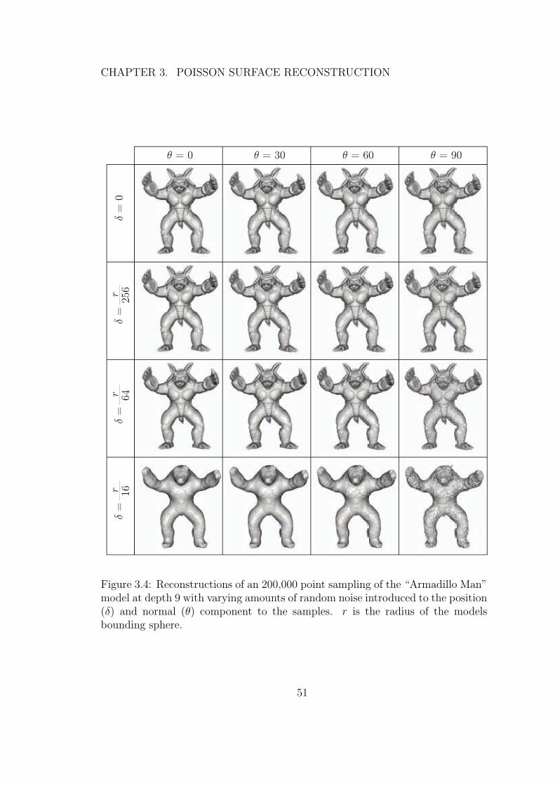
CHAPTER 3. POISSON SURFACE RECONSTRUCTION
± =
0
µ = 0 µ = 30 µ = 60 µ = 90
256r
± =
64r ±
=16r
± =
Figure 3.4: Reconstructions of an 200,000 point sampling of the “Armadillo Man”model at depth 9 with varying amounts of random noise introduced to the position(δ) and normal (θ) component to the samples. r is the radius of the modelsbounding sphere.
51
CHAPTER 3. POISSON SURFACE RECONSTRUCTION
amounts of positional noise, parts of the model begin to disconnect (e.g. the ears
and tail).
In addition to being robust to synthetic noise, the results in the rest of this
chapter also highlight our method’s ability to perform well with the types of noise
and other anomalies found in real-world scan data.
3.4.2 Comparison to Previous Work
In order to provide a context for evaluating the performance and reconstruction
abilities of our method, we compare the results of our algorithm to the results
obtained using Power Crust [4], Robust Cocone [18], Fast Radial Basis Functions
(FastRBF) [13], Multi-Level Partition of Unity Implicits (MPU) [43], Surface
Reconstruction from Unorganized Points [25], Volumetric Range Image Processing
(VRIP) [17], the Wavelet-based method of [39], and the FFT-based method of [31].
Our initial test case is the Stanford Bunny raw dataset of 362,000 points
assembled from ten range images. The data was processed to fit the input format
of each algorithm. For example, when running our method, we estimated a
sample’s normal from the positions of its neighbors. Running VRIP, we used
the registered scans as input, maintaining the regularity of the sampling, and
providing the confidence values.
Figure 3.5 compares the different reconstructions. Since the scanned data
contains noise, interpolatory methods such as Power Crust (a) and Robust Cocone
52
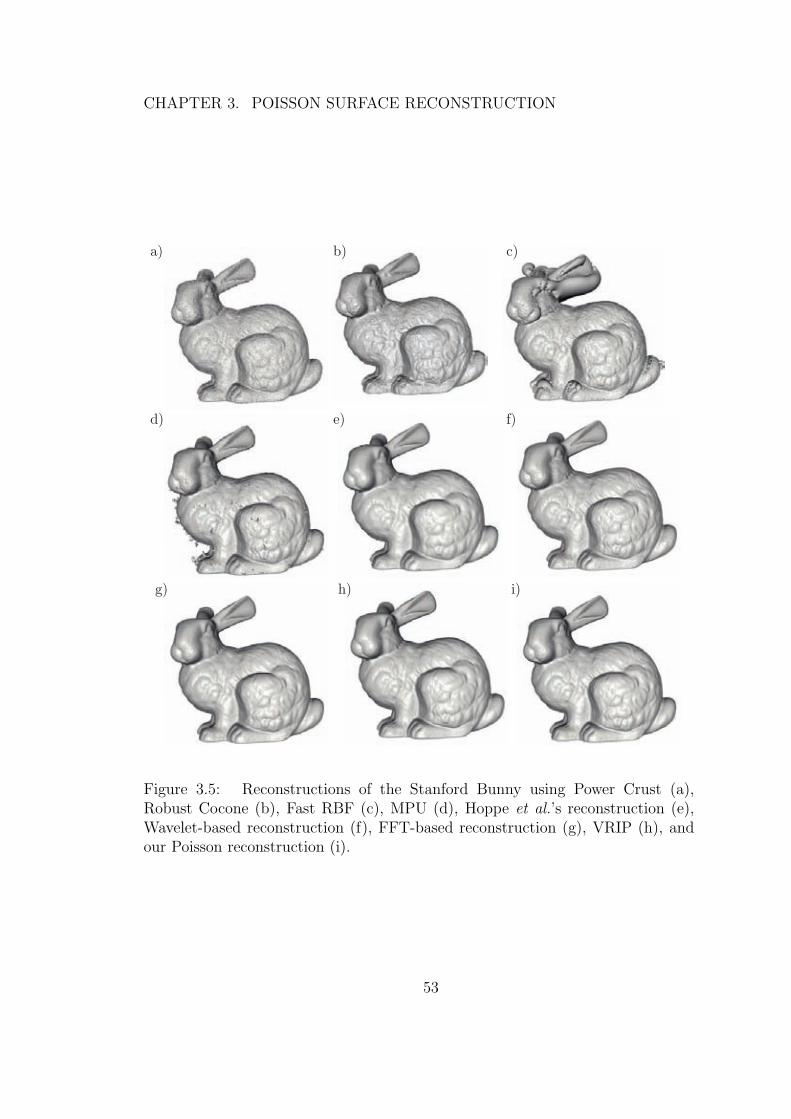
CHAPTER 3. POISSON SURFACE RECONSTRUCTION
a) b) c)
d) e) f)
g) h) i)
Figure 3.5: Reconstructions of the Stanford Bunny using Power Crust (a),Robust Cocone (b), Fast RBF (c), MPU (d), Hoppe et al.’s reconstruction (e),Wavelet-based reconstruction (f), FFT-based reconstruction (g), VRIP (h), andour Poisson reconstruction (i).
53
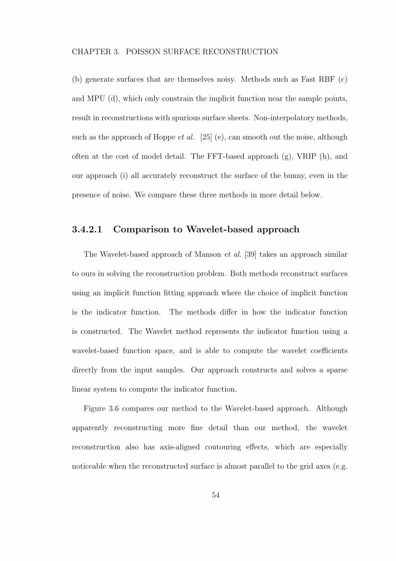
CHAPTER 3. POISSON SURFACE RECONSTRUCTION
(b) generate surfaces that are themselves noisy. Methods such as Fast RBF (c)
and MPU (d), which only constrain the implicit function near the sample points,
result in reconstructions with spurious surface sheets. Non-interpolatory methods,
such as the approach of Hoppe et al. [25] (e), can smooth out the noise, although
often at the cost of model detail. The FFT-based approach (g), VRIP (h), and
our approach (i) all accurately reconstruct the surface of the bunny, even in the
presence of noise. We compare these three methods in more detail below.
3.4.2.1 Comparison to Wavelet-based approach
The Wavelet-based approach of Manson et al. [39] takes an approach similar
to ours in solving the reconstruction problem. Both methods reconstruct surfaces
using an implicit function fitting approach where the choice of implicit function
is the indicator function. The methods differ in how the indicator function
is constructed. The Wavelet method represents the indicator function using a
wavelet-based function space, and is able to compute the wavelet coefficients
directly from the input samples. Our approach constructs and solves a sparse
linear system to compute the indicator function.
Figure 3.6 compares our method to the Wavelet-based approach. Although
apparently reconstructing more fine detail than our method, the wavelet
reconstruction also has axis-aligned contouring effects, which are especially
noticeable when the reconstructed surface is almost parallel to the grid axes (e.g.
54
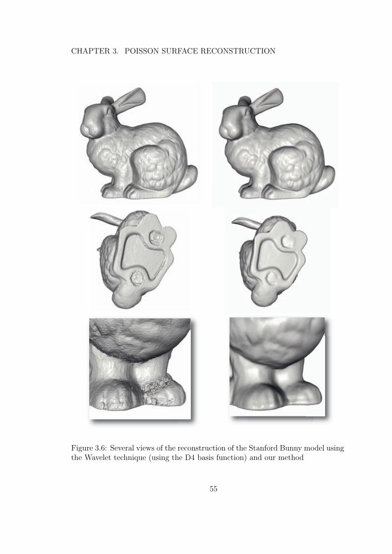
CHAPTER 3. POISSON SURFACE RECONSTRUCTION
Figure 3.6: Several views of the reconstruction of the Stanford Bunny model usingthe Wavelet technique (using the D4 basis function) and our method
55
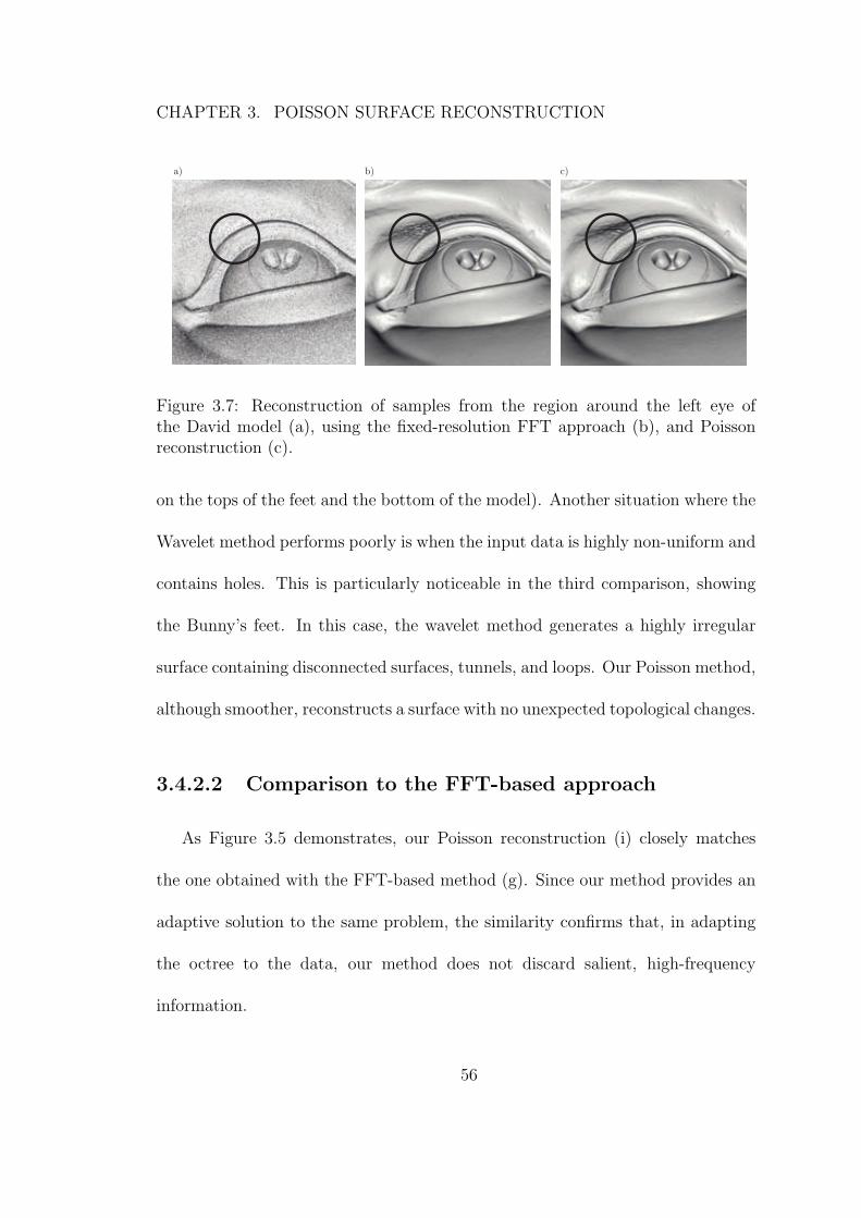
CHAPTER 3. POISSON SURFACE RECONSTRUCTION
a) b) c)
Figure 3.7: Reconstruction of samples from the region around the left eye ofthe David model (a), using the fixed-resolution FFT approach (b), and Poissonreconstruction (c).
on the tops of the feet and the bottom of the model). Another situation where the
Wavelet method performs poorly is when the input data is highly non-uniform and
contains holes. This is particularly noticeable in the third comparison, showing
the Bunny’s feet. In this case, the wavelet method generates a highly irregular
surface containing disconnected surfaces, tunnels, and loops. Our Poisson method,
although smoother, reconstructs a surface with no unexpected topological changes.
3.4.2.2 Comparison to the FFT-based approach
As Figure 3.5 demonstrates, our Poisson reconstruction (i) closely matches
the one obtained with the FFT-based method (g). Since our method provides an
adaptive solution to the same problem, the similarity confirms that, in adapting
the octree to the data, our method does not discard salient, high-frequency
information.
56
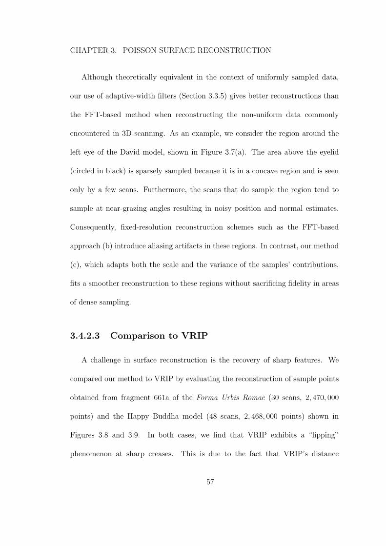
CHAPTER 3. POISSON SURFACE RECONSTRUCTION
Although theoretically equivalent in the context of uniformly sampled data,
our use of adaptive-width filters (Section 3.3.5) gives better reconstructions than
the FFT-based method when reconstructing the non-uniform data commonly
encountered in 3D scanning. As an example, we consider the region around the
left eye of the David model, shown in Figure 3.7(a). The area above the eyelid
(circled in black) is sparsely sampled because it is in a concave region and is seen
only by a few scans. Furthermore, the scans that do sample the region tend to
sample at near-grazing angles resulting in noisy position and normal estimates.
Consequently, fixed-resolution reconstruction schemes such as the FFT-based
approach (b) introduce aliasing artifacts in these regions. In contrast, our method
(c), which adapts both the scale and the variance of the samples’ contributions,
fits a smoother reconstruction to these regions without sacrificing fidelity in areas
of dense sampling.
3.4.2.3 Comparison to VRIP
A challenge in surface reconstruction is the recovery of sharp features. We
compared our method to VRIP by evaluating the reconstruction of sample points
obtained from fragment 661a of the Forma Urbis Romae (30 scans, 2, 470, 000
points) and the Happy Buddha model (48 scans, 2, 468, 000 points) shown in
Figures 3.8 and 3.9. In both cases, we find that VRIP exhibits a “lipping”
phenomenon at sharp creases. This is due to the fact that VRIP’s distance
57
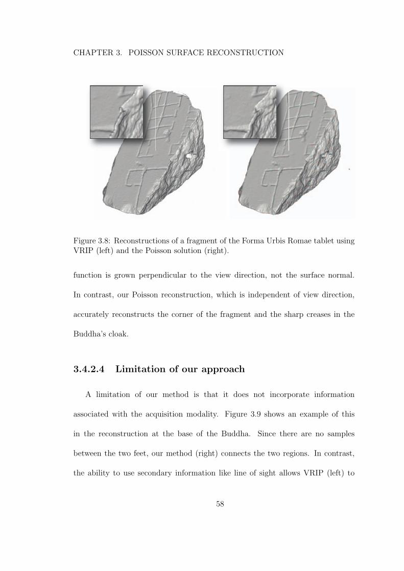
CHAPTER 3. POISSON SURFACE RECONSTRUCTION
Figure 3.8: Reconstructions of a fragment of the Forma Urbis Romae tablet usingVRIP (left) and the Poisson solution (right).
function is grown perpendicular to the view direction, not the surface normal.
In contrast, our Poisson reconstruction, which is independent of view direction,
accurately reconstructs the corner of the fragment and the sharp creases in the
Buddha’s cloak.
3.4.2.4 Limitation of our approach
A limitation of our method is that it does not incorporate information
associated with the acquisition modality. Figure 3.9 shows an example of this
in the reconstruction at the base of the Buddha. Since there are no samples
between the two feet, our method (right) connects the two regions. In contrast,
the ability to use secondary information like line of sight allows VRIP (left) to
58
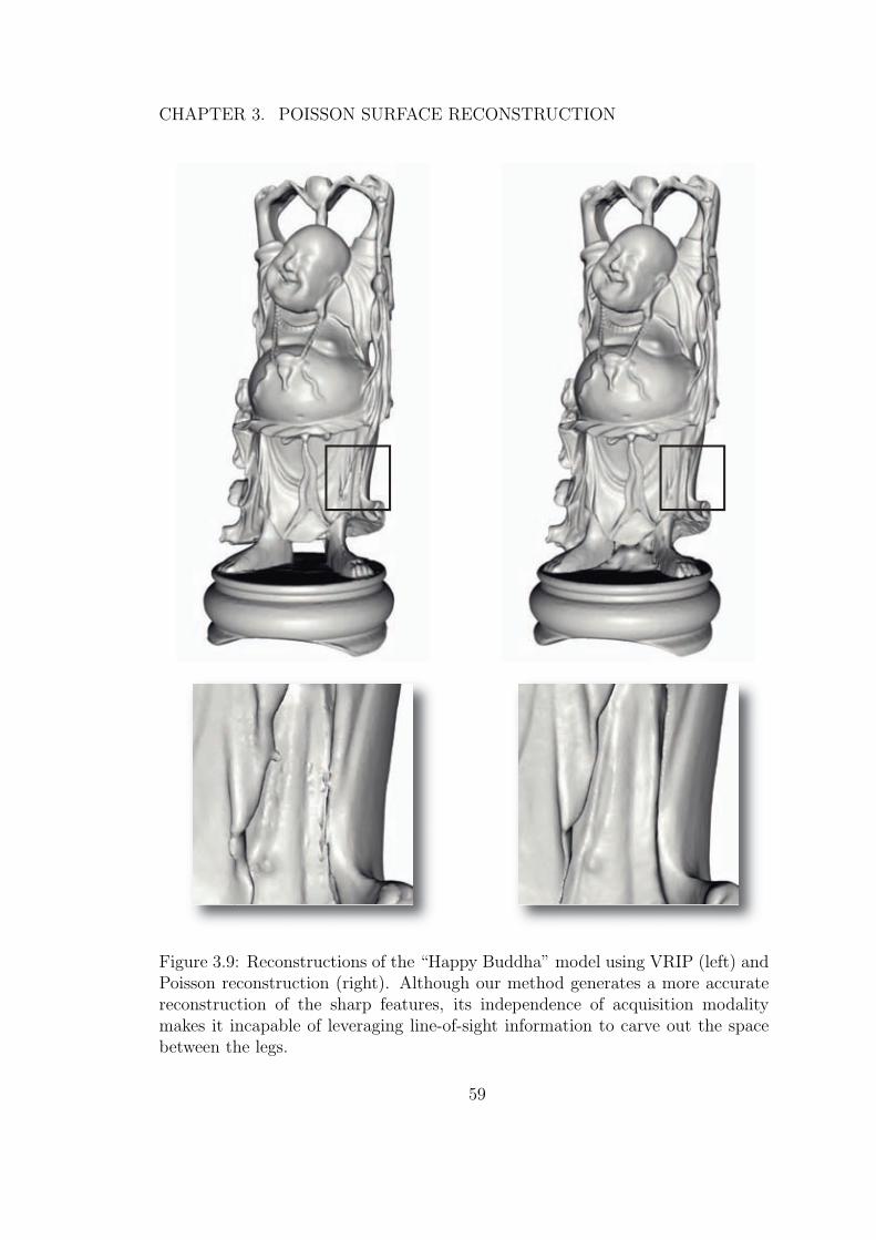
CHAPTER 3. POISSON SURFACE RECONSTRUCTION
Figure 3.9: Reconstructions of the “Happy Buddha” model using VRIP (left) andPoisson reconstruction (right). Although our method generates a more accuratereconstruction of the sharp features, its independence of acquisition modalitymakes it incapable of leveraging line-of-sight information to carve out the spacebetween the legs.
59
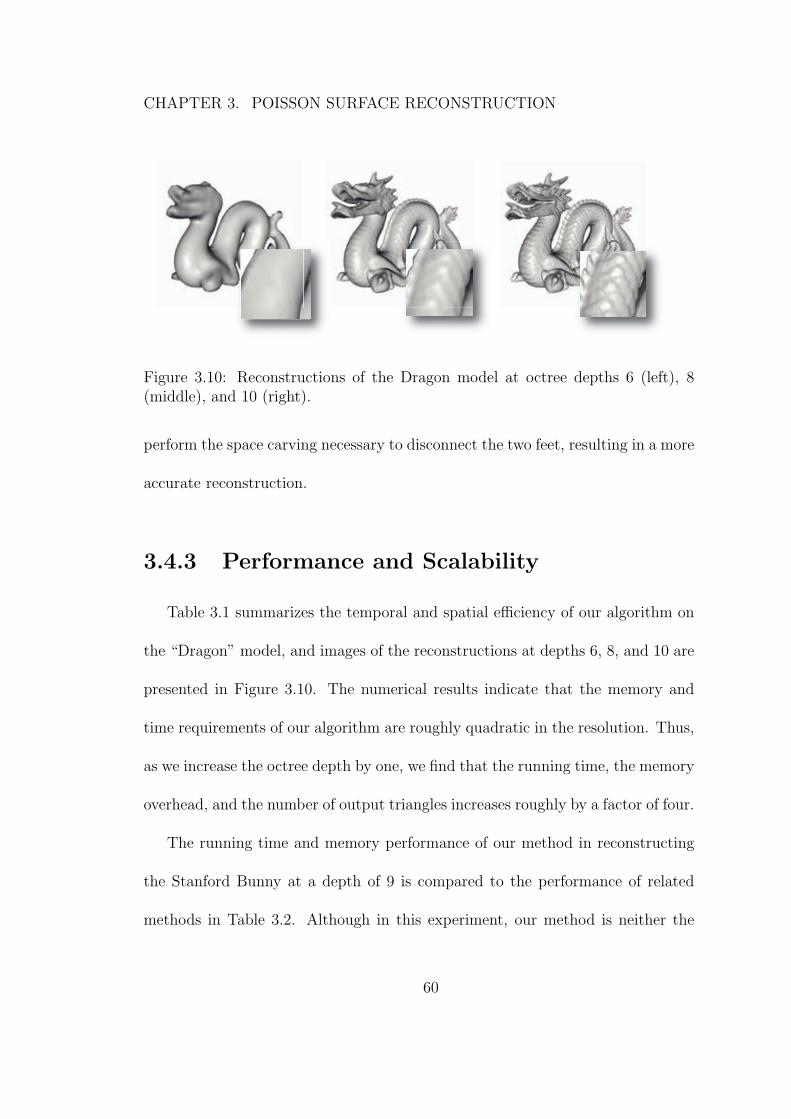
CHAPTER 3. POISSON SURFACE RECONSTRUCTION
Figure 3.10: Reconstructions of the Dragon model at octree depths 6 (left), 8(middle), and 10 (right).
perform the space carving necessary to disconnect the two feet, resulting in a more
accurate reconstruction.
3.4.3 Performance and Scalability
Table 3.1 summarizes the temporal and spatial efficiency of our algorithm on
the “Dragon” model, and images of the reconstructions at depths 6, 8, and 10 are
presented in Figure 3.10. The numerical results indicate that the memory and
time requirements of our algorithm are roughly quadratic in the resolution. Thus,
as we increase the octree depth by one, we find that the running time, the memory
overhead, and the number of output triangles increases roughly by a factor of four.
The running time and memory performance of our method in reconstructing
the Stanford Bunny at a depth of 9 is compared to the performance of related
methods in Table 3.2. Although in this experiment, our method is neither the
60
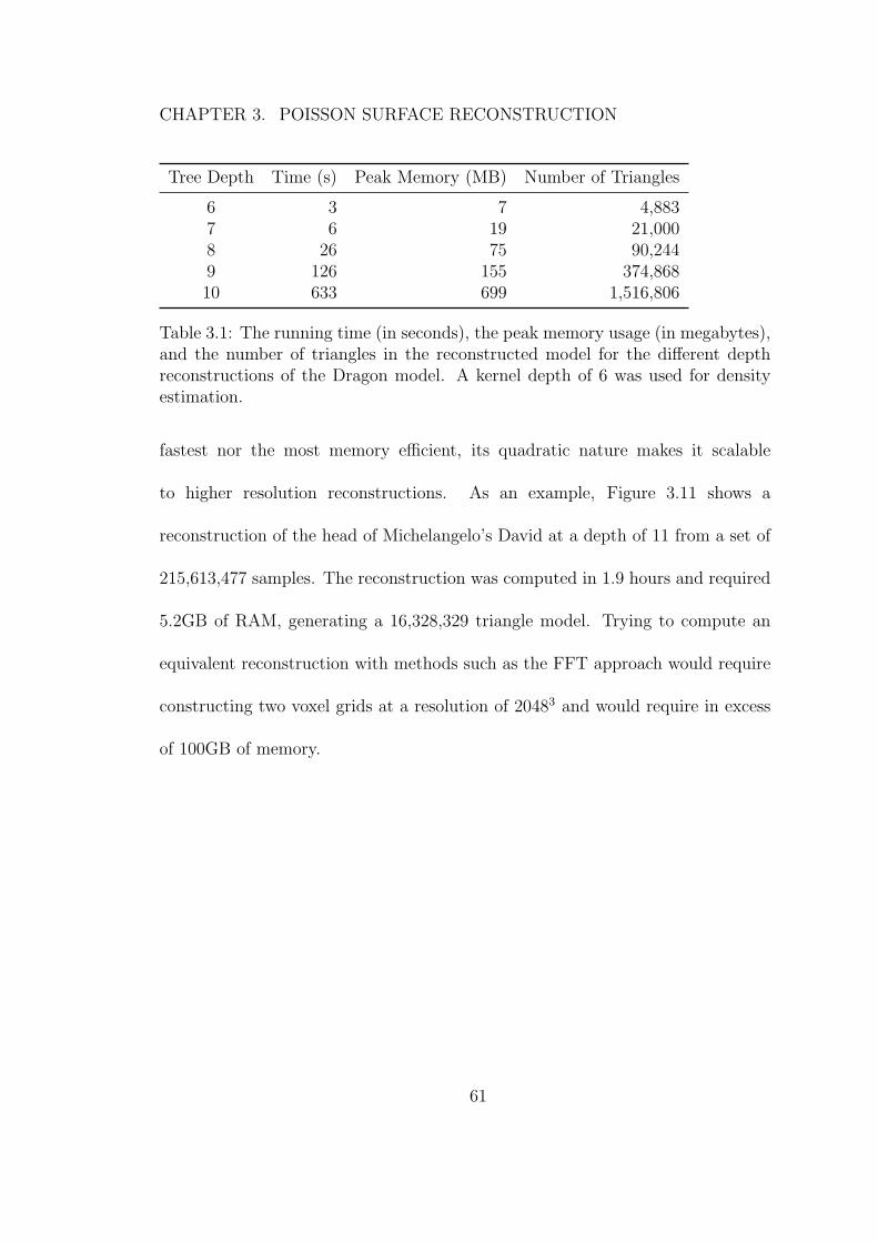
CHAPTER 3. POISSON SURFACE RECONSTRUCTION
Tree Depth Time (s) Peak Memory (MB) Number of Triangles
6 3 7 4,8837 6 19 21,0008 26 75 90,2449 126 155 374,86810 633 699 1,516,806
Table 3.1: The running time (in seconds), the peak memory usage (in megabytes),and the number of triangles in the reconstructed model for the different depthreconstructions of the Dragon model. A kernel depth of 6 was used for densityestimation.
fastest nor the most memory efficient, its quadratic nature makes it scalable
to higher resolution reconstructions. As an example, Figure 3.11 shows a
reconstruction of the head of Michelangelo’s David at a depth of 11 from a set of
215,613,477 samples. The reconstruction was computed in 1.9 hours and required
5.2GB of RAM, generating a 16,328,329 triangle model. Trying to compute an
equivalent reconstruction with methods such as the FFT approach would require
constructing two voxel grids at a resolution of 20483 and would require in excess
of 100GB of memory.
61
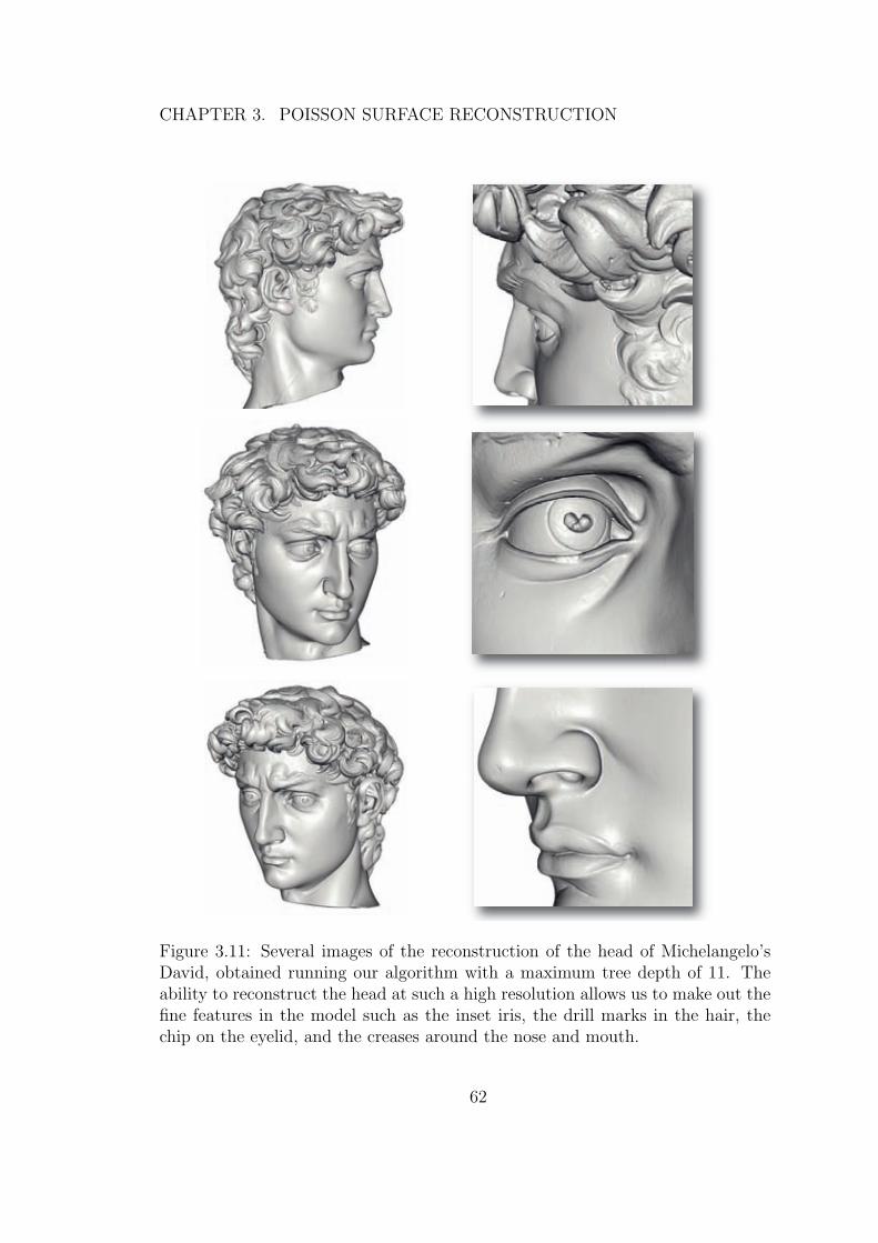
CHAPTER 3. POISSON SURFACE RECONSTRUCTION
Figure 3.11: Several images of the reconstruction of the head of Michelangelo’sDavid, obtained running our algorithm with a maximum tree depth of 11. Theability to reconstruct the head at such a high resolution allows us to make out thefine features in the model such as the inset iris, the drill marks in the hair, thechip on the eyelid, and the creases around the nose and mouth.
62
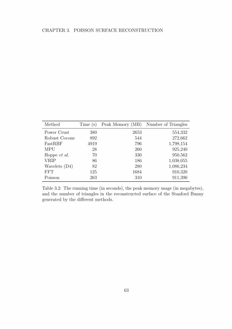
CHAPTER 3. POISSON SURFACE RECONSTRUCTION
Method Time (s) Peak Memory (MB) Number of Triangles
Power Crust 380 2653 554,332Robust Cocone 892 544 272,662FastRBF 4919 796 1,798,154MPU 28 260 925,240Hoppe et al. 70 330 950,562VRIP 86 186 1,038,055Wavelets (D4) 82 280 1,086,234FFT 125 1684 910,320Poisson 263 310 911,390
Table 3.2: The running time (in seconds), the peak memory usage (in megabytes),and the number of triangles in the reconstructed surface of the Stanford Bunnygenerated by the different methods.
63
Chapter 4
Streaming Surface
Reconstruction
In Chapter 3, we demonstrated that surface reconstruction from oriented
points can be made more resilient to data errors by casting the problem as a
global Poisson system. Intuitively, the idea is to interpret the oriented points as
samples of the gradient of the model’s indicator function χ (defined as 1 at points
inside the model, and 0 at points outside). Thus, the desired indicator function
is the one whose Laplacian equals the divergence of a vector field ~V constructed
from the oriented points: ∆χ = ∇ · ~V . By representing χ using a basis defined
over an adaptive octree, the Poisson equation is discretized into a sparse linear
system L x = b where the size of the system is proportional to the complexity of
the reconstructed surface. Then, the desired model is extracted as an iso-surface
64
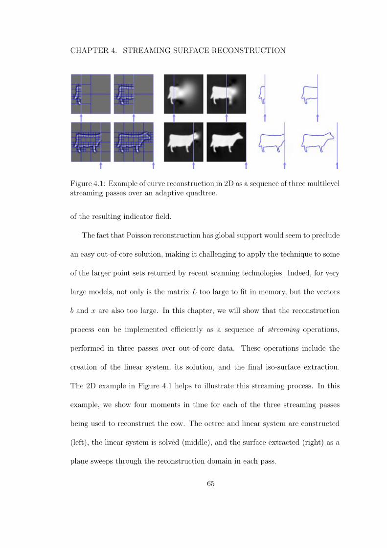
CHAPTER 4. STREAMING SURFACE RECONSTRUCTION
Figure 4.1: Example of curve reconstruction in 2D as a sequence of three multilevelstreaming passes over an adaptive quadtree.
of the resulting indicator field.
The fact that Poisson reconstruction has global support would seem to preclude
an easy out-of-core solution, making it challenging to apply the technique to some
of the larger point sets returned by recent scanning technologies. Indeed, for very
large models, not only is the matrix L too large to fit in memory, but the vectors
b and x are also too large. In this chapter, we will show that the reconstruction
process can be implemented efficiently as a sequence of streaming operations,
performed in three passes over out-of-core data. These operations include the
creation of the linear system, its solution, and the final iso-surface extraction.
The 2D example in Figure 4.1 helps to illustrate this streaming process. In this
example, we show four moments in time for each of the three streaming passes
being used to reconstruct the cow. The octree and linear system are constructed
(left), the linear system is solved (middle), and the surface extracted (right) as a
plane sweeps through the reconstruction domain in each pass.
65
CHAPTER 4. STREAMING SURFACE RECONSTRUCTION
In general, a streaming approach is advantageous because data is accessed
sequentially from disk, and it is only loaded once. Sequential access is typically
more efficient because it allows for data prefetching. In computer graphics,
streaming computation has been performed over many data types including
triangle meshes, point sets and tetrahedral meshes, as reviewed in Section 4.1.
A unique aspect of our problem is the requirement for an adaptive
multiresolution structure, namely an octree, because a solution over a uniform
3D grid is not scalable [31]. Interestingly, the operations performed on the octree
have different types of inter-level data dependencies and, consequently, no single
linear ordering of the octree nodes is adequate. To overcome these dependencies,
we introduce a multilevel streaming representation in which each level is stored
as a separate stream. A processing pass sweeps over the octree by concurrently
advancing through the multiple streams, iterating at a faster rate through the
finer nodes than the coarser ones. Depending on the operation, information flows
up and/or down the tree, and computations on coarser levels precede or succeed
those on finer levels.
A surprising result is that we are able to solve the sparse Poisson system
L x = b with sufficient accuracy for our reconstruction application in only two
multi-stream passes through the data; one pass to compute the divergence, and
a second pass to solve the linear system. We are able to do this in two passes
thorugh the data because clever scheduling of the computation across levels lets us
66
CHAPTER 4. STREAMING SURFACE RECONSTRUCTION
realize a multigrid scheme using Gauss-Seidel updates [11], enabling sufficiently
accurate convergence using only local updates.
Using this method, we are able to obtain reconstructions of highly complex
models (210 million triangles) on a PC with only 1 GB of memory, and
demonstrate scalable performance.
4.1 Related Work
4.1.1 Out-of-core Surface Reconstruction
Several surface reconstruction algorithms lend themselves naturally to out-of-
core computation because their access patterns are highly localized. For instance,
the range-image volumetric merging scheme of Curless and Levoy [17] can easily
be computed independently on blocks of the domain space. For each block,
one conservatively finds the scanned points that can contribute to it. Schemes
based on local neighborhood fitting such as [3, 25] could also be computed in a
streaming traversal, for instance using the scheme of Pajarola [44]. The multilevel
partition of unity (MPU) approach of [43] uses an adaptive octree structure to
blend together estimated implicit surface patches. Its use of local weights should
make it amenable to out-of-core processing. The ball-pivoting algorithm of [8] is
implemented out-of-core by partitioning the domain into slices.
Our work is the first to present an out-of-core implementation of a global
67
CHAPTER 4. STREAMING SURFACE RECONSTRUCTION
surface reconstruction technique.
4.1.2 Stream Processing
Much of the streaming work in computer graphics focuses on irregular triangle
meshes [2, 6, 27, 29, 56]. Streaming operations include surface smoothing, mesh
simplification, remeshing, and normal estimation. Streaming has also been
applied to irregular tetrahedral mesh compression [30] and simplification [53].
Pajarola [44] describes stream processing on points. His streaming scheme is able
to find the k-closest neighborhoods of the points, to enable processing operations
such as density computation, normal estimation, and geometric smoothing.
Isenburg et al. [28] stream through a set of points to incrementally construct
a Delaunay triangulation. Whereas prior streaming methods operate at a single
resolution on the data, we introduce a multiresolution streaming framework.
4.1.3 Other Out-of-core Processing
Cignoni et al. [16] introduce an octree-based external memory structure to
store an irregular mesh out-of-core. They describe how to handle triangles that
span octree cell boundaries. Processing a subtree involves loading its adjacent leaf-
nodes into memory. Maintaining random access to the octree nodes is beneficial
for view-dependent rendering, as also shown in [36].
68
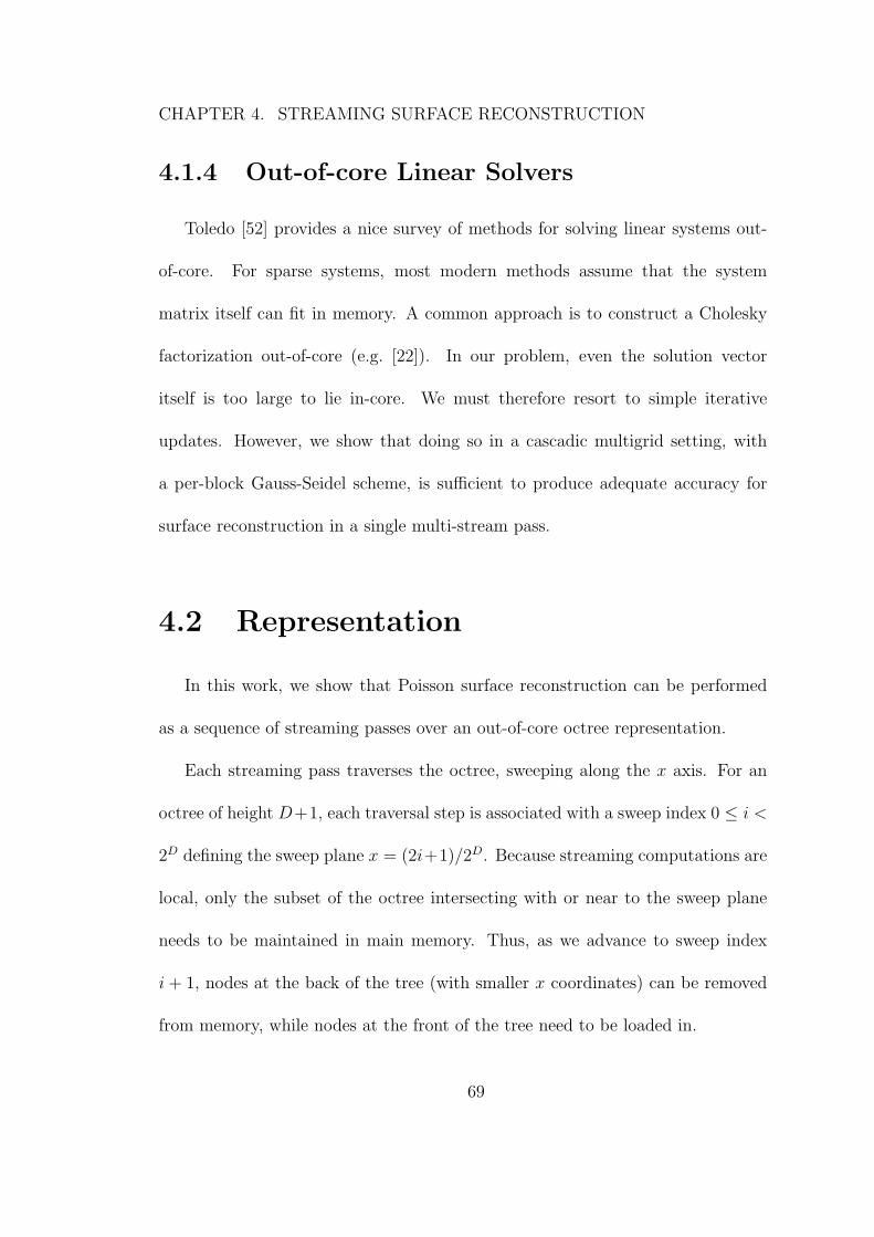
CHAPTER 4. STREAMING SURFACE RECONSTRUCTION
4.1.4 Out-of-core Linear Solvers
Toledo [52] provides a nice survey of methods for solving linear systems out-
of-core. For sparse systems, most modern methods assume that the system
matrix itself can fit in memory. A common approach is to construct a Cholesky
factorization out-of-core (e.g. [22]). In our problem, even the solution vector
itself is too large to lie in-core. We must therefore resort to simple iterative
updates. However, we show that doing so in a cascadic multigrid setting, with
a per-block Gauss-Seidel scheme, is sufficient to produce adequate accuracy for
surface reconstruction in a single multi-stream pass.
4.2 Representation
In this work, we show that Poisson surface reconstruction can be performed
as a sequence of streaming passes over an out-of-core octree representation.
Each streaming pass traverses the octree, sweeping along the x axis. For an
octree of height D+1, each traversal step is associated with a sweep index 0 ≤ i <
2D defining the sweep plane x = (2i+1)/2D. Because streaming computations are
local, only the subset of the octree intersecting with or near to the sweep plane
needs to be maintained in main memory. Thus, as we advance to sweep index
i + 1, nodes at the back of the tree (with smaller x coordinates) can be removed
from memory, while nodes at the front of the tree need to be loaded in.
69
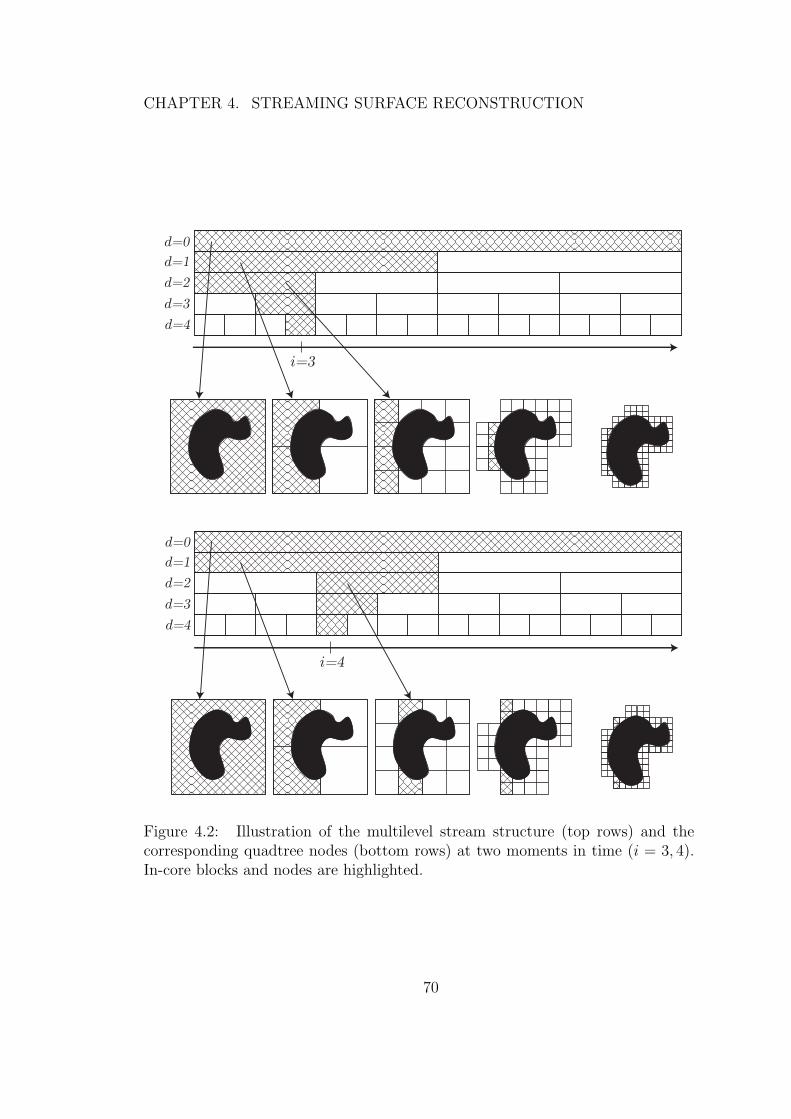
CHAPTER 4. STREAMING SURFACE RECONSTRUCTION
d=0
d=1
d=2
d=3
d=4
i=3
d=0
d=1
d=2
d=3
d=4
i=4
Figure 4.2: Illustration of the multilevel stream structure (top rows) and thecorresponding quadtree nodes (bottom rows) at two moments in time (i = 3, 4).In-core blocks and nodes are highlighted.
70
CHAPTER 4. STREAMING SURFACE RECONSTRUCTION
To implement a data structure that supports this traversal pattern, we must
address the fact that the in-core persistence of nodes depends on their depth, since
coarser nodes are maintained in memory longer than finer ones (see Figure 4.2).
This motivates the construction of a multi-stream octree data structure, consisting
of D + 1 different streams {S0, . . . ,SD}.
Each stream Sd contains all nodes o ∈ Od, and is partitioned into blocks
Sd[0], . . . ,Sd[2d − 1] with the nodes in block Sd[j] all centered on the plane x =
(2j+1)/2d+1. Thus, at the coarsest depth, S0 contains only one block S0[0] which
in turn contains only one node, namely the octree root node. At finer depths, each
block Sd[j] generally contains O(2d) nodes (out of 22d nodes in a complete octree)
because the surface has co-dimension 1.
Figure 4.2 shows a visualization of the multi-stream structure for a quadtree
representation. Each row marked with a depth d = 0 . . . 4 corresponds to a
separate stream Sd, and the rectangles within a row denote the blocks Sd[j]. In
the top two rows of the diagram, we see the data structure at sweep index i = 3.
The in-core blocks which correspond to all the quadtree nodes that intersect the
sweep-plane are highlighted. Note that as we advance to sweep index i = 4 (shown
in bottom two rows), not all streams need to be updated; in this example, it is
only the streams at depths d = 2, 3, 4 that are advanced.
At index i, the sweep plane intersects the nodes contained in Sd[bi/2D−d−1c],
which we denote by Sd[φd(i)], or simply as Sdi . More generally, stream processing
71
CHAPTER 4. STREAMING SURFACE RECONSTRUCTION
operations may require access to nodes in a small neighborhood of the sweep plane.
If the operation needs access to a k-neighborhood at each depth, we maintain an
in-core octree Oi,k ⊂ O defined as the union
Oi,k =D⋃
d=0
Sdi,k where Sd
i,k =k⋃
j=−k
Sd[φd(i) + j]. (4.1)
Thus, Figure 4.2 can be seen to correspond to Oi,0 at i = 3, 4.
An essential property of the in-core octree is that for any node o ∈ Sdi and
any depth d′ ≤ d, the k-neighborhood of the ancestor of o at depth d′, denoted
Nd′
k (o), is guaranteed to be contained in Oi,k, (i.e. to be in-core). As the sweep
index is advanced from i to i + 1, the in-core octree Oi,k is updated. Specifically,
we compute the set of depths, Di, at which the streams need to be advanced:
Di = {d | φd(i) 6= φd(i + 1)} (4.2)
and for each d ∈ Di we can unload the block Sd[φd(i) − k] and load the block
Sd[φd(i) + k + 1] into memory.
4.2.1 Implementation
We store each stream in a separate file, and using a 64-bit operating system,
reserve contiguous blocks of virtual address space large enough to fully span the
streams. An advantage of using virtual addressing is that, by simple addition with
72
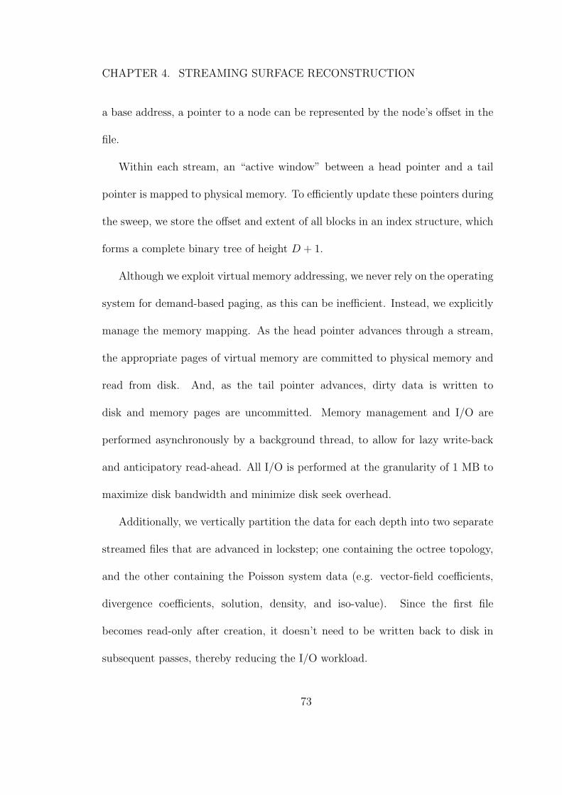
CHAPTER 4. STREAMING SURFACE RECONSTRUCTION
a base address, a pointer to a node can be represented by the node’s offset in the
file.
Within each stream, an “active window” between a head pointer and a tail
pointer is mapped to physical memory. To efficiently update these pointers during
the sweep, we store the offset and extent of all blocks in an index structure, which
forms a complete binary tree of height D + 1.
Although we exploit virtual memory addressing, we never rely on the operating
system for demand-based paging, as this can be inefficient. Instead, we explicitly
manage the memory mapping. As the head pointer advances through a stream,
the appropriate pages of virtual memory are committed to physical memory and
read from disk. And, as the tail pointer advances, dirty data is written to
disk and memory pages are uncommitted. Memory management and I/O are
performed asynchronously by a background thread, to allow for lazy write-back
and anticipatory read-ahead. All I/O is performed at the granularity of 1 MB to
maximize disk bandwidth and minimize disk seek overhead.
Additionally, we vertically partition the data for each depth into two separate
streamed files that are advanced in lockstep; one containing the octree topology,
and the other containing the Poisson system data (e.g. vector-field coefficients,
divergence coefficients, solution, density, and iso-value). Since the first file
becomes read-only after creation, it doesn’t need to be written back to disk in
subsequent passes, thereby reducing the I/O workload.
73
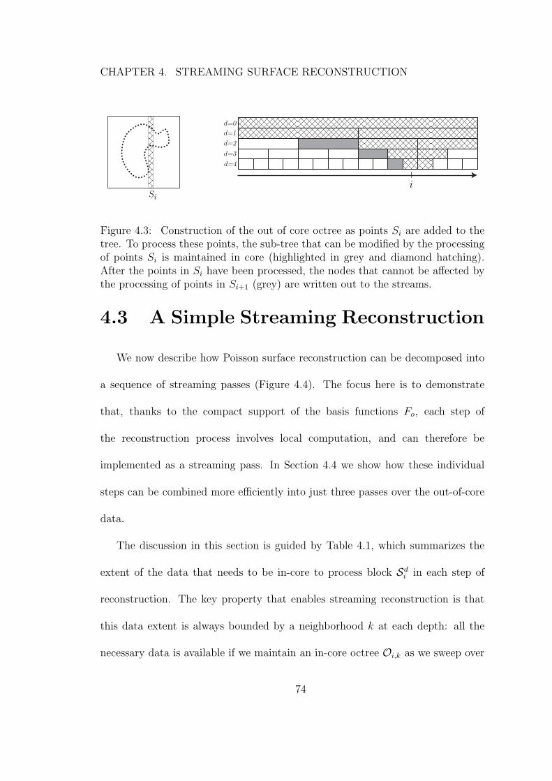
CHAPTER 4. STREAMING SURFACE RECONSTRUCTION
d=0
d=1
d=2
d=3
d=4
iSi
Figure 4.3: Construction of the out of core octree as points Si are added to thetree. To process these points, the sub-tree that can be modified by the processingof points Si is maintained in core (highlighted in grey and diamond hatching).After the points in Si have been processed, the nodes that cannot be affected bythe processing of points in Si+1 (grey) are written out to the streams.
4.3 A Simple Streaming Reconstruction
We now describe how Poisson surface reconstruction can be decomposed into
a sequence of streaming passes (Figure 4.4). The focus here is to demonstrate
that, thanks to the compact support of the basis functions Fo, each step of
the reconstruction process involves local computation, and can therefore be
implemented as a streaming pass. In Section 4.4 we show how these individual
steps can be combined more efficiently into just three passes over the out-of-core
data.
The discussion in this section is guided by Table 4.1, which summarizes the
extent of the data that needs to be in-core to process block Sdi in each step of
reconstruction. The key property that enables streaming reconstruction is that
this data extent is always bounded by a neighborhood k at each depth: all the
necessary data is available if we maintain an in-core octree Oi,k as we sweep over
74
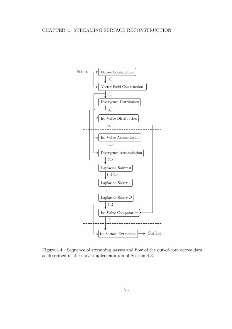
CHAPTER 4. STREAMING SURFACE RECONSTRUCTION
Points
fkog
Surface
Vector Field Construction
vof g
xof g
bof gxof g
Divergence Accumulation
Octree Construction
Iso-Value Computation
Iso-Surface Extraction
Laplacian Solver D
Laplacian Solver 1
Laplacian Solver 0
...
Divergence Distribution
Iso-Value Distribution
Iso-Value Accumulation
bof g
°of g
°of g
¡
bof g
Figure 4.4: Sequence of streaming passes and flow of the out-of-core octree data,as described in the naive implementation of Section 4.3.
75
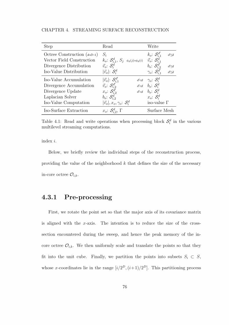
CHAPTER 4. STREAMING SURFACE RECONSTRUCTION
Step Read Write
Octree Construction (d=D−1) Si ko: Sd′i,1 d′≤d
Vector Field Construction ko: Sdi,1, Sj φd(j)=φd(i) ~vo: Sd
i,1
Divergence Distribution ~vo: Sdi bo: Sd′
i,2 d′≤d
Iso-Value Distribution |~vo|: Sdi γo: Sd′
i,1 d′≤d
Iso-Value Accumulation |~vo|: Sd′i,1 d′<d γo: Sd
i
Divergence Accumulation ~vo: Sd′i,2 d′<d bo: Sd
i
Divergence Update xo: Sd′i,2 d′<d bo: Sd
i
Laplacian Solver bo: Sdi,2 xo: Sd
i
Iso-Value Computation |~vo|, xo, γo: Sdi iso-value Γ
Iso-Surface Extraction xo: Sdi,2, Γ Surface Mesh
Table 4.1: Read and write operations when processing block Sdi in the various
multilevel streaming computations.
index i.
Below, we briefly review the individual steps of the reconstruction process,
providing the value of the neighborhood k that defines the size of the necessary
in-core octree Oi,k.
4.3.1 Pre-processing
First, we rotate the point set so that the major axis of its covariance matrix
is aligned with the x-axis. The intention is to reduce the size of the cross-
section encountered during the sweep, and hence the peak memory of the in-
core octree Oi,k. We then uniformly scale and translate the points so that they
fit into the unit cube. Finally, we partition the points into subsets Si ⊂ S,
whose x-coordinates lie in the range [i/2D, (i+1)/2D]. This partitioning process
76
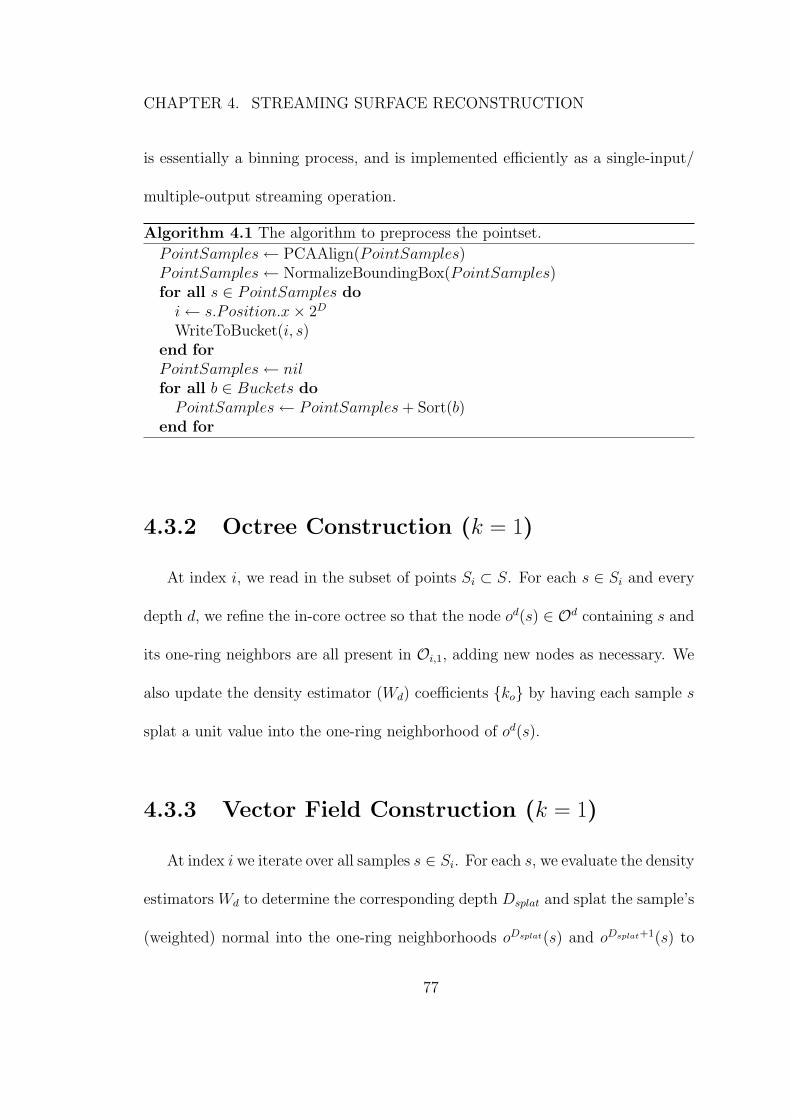
CHAPTER 4. STREAMING SURFACE RECONSTRUCTION
is essentially a binning process, and is implemented efficiently as a single-input/
multiple-output streaming operation.
Algorithm 4.1 The algorithm to preprocess the pointset.
PointSamples← PCAAlign(PointSamples)PointSamples← NormalizeBoundingBox(PointSamples)for all s ∈ PointSamples do
i← s.Position.x× 2D
WriteToBucket(i, s)end forPointSamples← nilfor all b ∈ Buckets do
PointSamples← PointSamples + Sort(b)end for
4.3.2 Octree Construction (k = 1)
At index i, we read in the subset of points Si ⊂ S. For each s ∈ Si and every
depth d, we refine the in-core octree so that the node od(s) ∈ Od containing s and
its one-ring neighbors are all present in Oi,1, adding new nodes as necessary. We
also update the density estimator (Wd) coefficients {ko} by having each sample s
splat a unit value into the one-ring neighborhood of od(s).
4.3.3 Vector Field Construction (k = 1)
At index i we iterate over all samples s ∈ Si. For each s, we evaluate the density
estimators Wd to determine the corresponding depth Dsplat and splat the sample’s
(weighted) normal into the one-ring neighborhoods oDsplat(s) and oDsplat+1(s) to
77
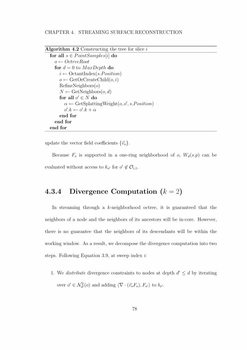
CHAPTER 4. STREAMING SURFACE RECONSTRUCTION
Algorithm 4.2 Constructing the tree for slice i
for all s ∈ PointSamples[i] doo← OctreeRootfor d = 0 to MaxDepth do
i← OctantIndex(s.Position)o← GetOrCreateChild(o, i)RefineNeighbors(o)N ← GetNeighbors(o, d)for all o′ ∈ N do
α← GetSplattingWeight(o, o′, s.Position)o′.k ← o′.k + α
end forend for
end for
update the vector field coefficients {~vo}.
Because Fo is supported in a one-ring neighborhood of o, Wd(s.p) can be
evaluated without access to ko′ for o′ 6∈ Oi,1.
4.3.4 Divergence Computation (k = 2)
In streaming through a k-neighborhood octree, it is guaranteed that the
neighbors of a node and the neighbors of its ancestors will be in-core. However,
there is no guarantee that the neighbors of its descendants will be within the
working window. As a result, we decompose the divergence computation into two
steps. Following Equation 3.9, at sweep index i:
1. We distribute divergence constraints to nodes at depth d′ ≤ d by iterating
over o′ ∈ N 2d′(o) and adding 〈∇ · (~voFo), Fo′〉 to bo′ .
78
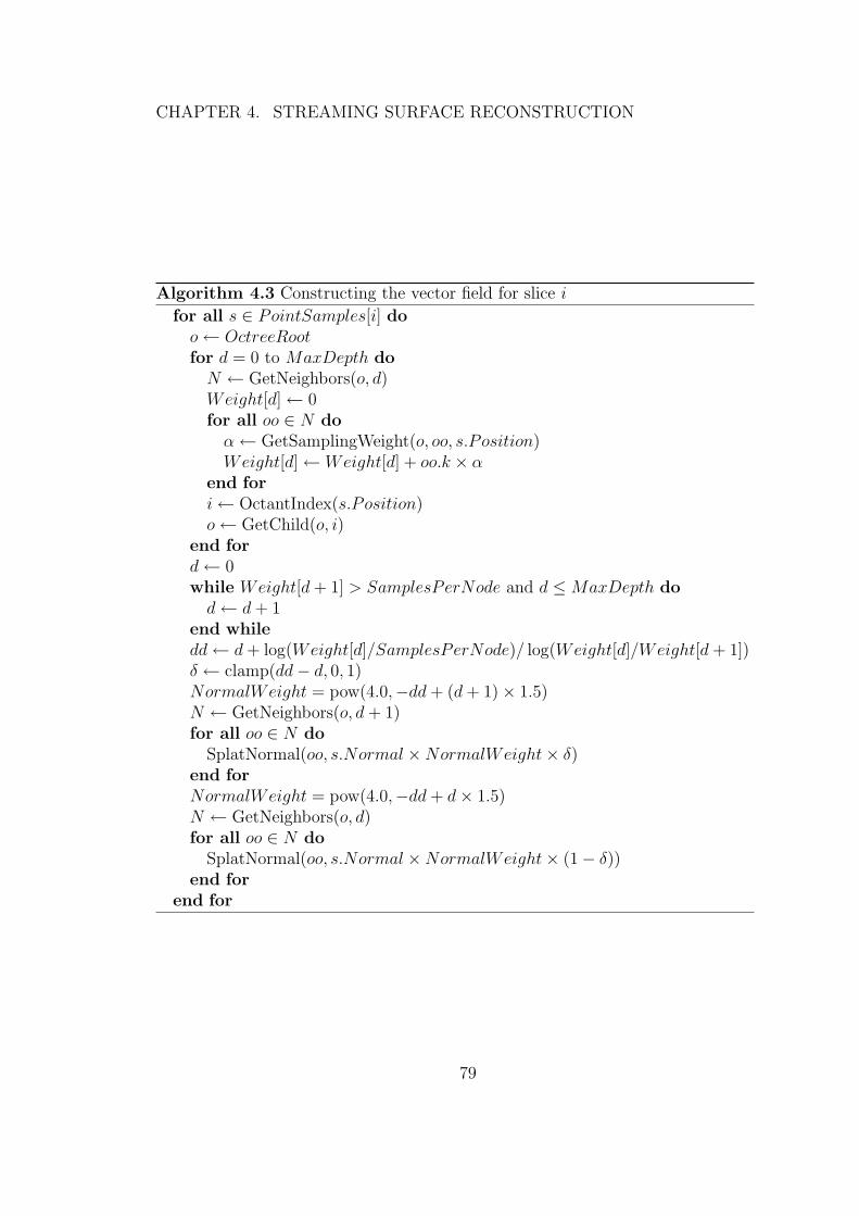
CHAPTER 4. STREAMING SURFACE RECONSTRUCTION
Algorithm 4.3 Constructing the vector field for slice i
for all s ∈ PointSamples[i] doo← OctreeRootfor d = 0 to MaxDepth do
N ← GetNeighbors(o, d)Weight[d]← 0for all oo ∈ N do
α← GetSamplingWeight(o, oo, s.Position)Weight[d]← Weight[d] + oo.k × α
end fori← OctantIndex(s.Position)o← GetChild(o, i)
end ford← 0while Weight[d + 1] > SamplesPerNode and d ≤MaxDepth do
d← d + 1end whiledd← d + log(Weight[d]/SamplesPerNode)/ log(Weight[d]/Weight[d + 1])δ ← clamp(dd− d, 0, 1)NormalWeight = pow(4.0,−dd + (d + 1)× 1.5)N ← GetNeighbors(o, d + 1)for all oo ∈ N do
SplatNormal(oo, s.Normal ×NormalWeight× δ)end forNormalWeight = pow(4.0,−dd + d× 1.5)N ← GetNeighbors(o, d)for all oo ∈ N do
SplatNormal(oo, s.Normal ×NormalWeight× (1− δ))end for
end for
79
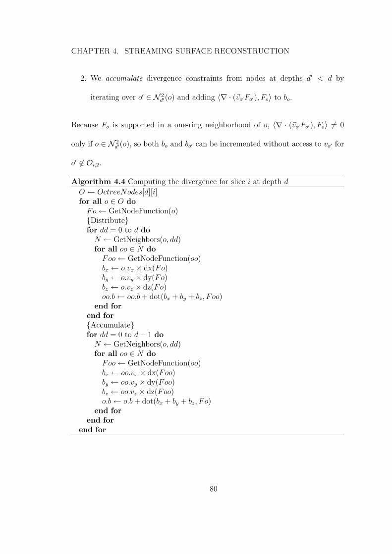
CHAPTER 4. STREAMING SURFACE RECONSTRUCTION
2. We accumulate divergence constraints from nodes at depths d′ < d by
iterating over o′ ∈ N 2d′(o) and adding 〈∇ · (~vo′Fo′), Fo〉 to bo.
Because Fo is supported in a one-ring neighborhood of o, 〈∇ · (~vo′Fo′), Fo〉 6= 0
only if o ∈ N 2d′(o), so both bo and bo′ can be incremented without access to vo′ for
o′ 6∈ Oi,2.
Algorithm 4.4 Computing the divergence for slice i at depth d
O ← OctreeNodes[d][i]for all o ∈ O do
Fo← GetNodeFunction(o){Distribute}for dd = 0 to d do
N ← GetNeighbors(o, dd)for all oo ∈ N do
Foo← GetNodeFunction(oo)bx ← o.vx × dx(Fo)by ← o.vy × dy(Fo)bz ← o.vz × dz(Fo)oo.b← oo.b + dot(bx + by + bz, Foo)
end forend for{Accumulate}for dd = 0 to d− 1 do
N ← GetNeighbors(o, dd)for all oo ∈ N do
Foo← GetNodeFunction(oo)bx ← oo.vx × dx(Foo)by ← oo.vy × dy(Foo)bz ← oo.vz × dz(Foo)o.b← o.b + dot(bx + by + bz, Fo)
end forend for
end for
80
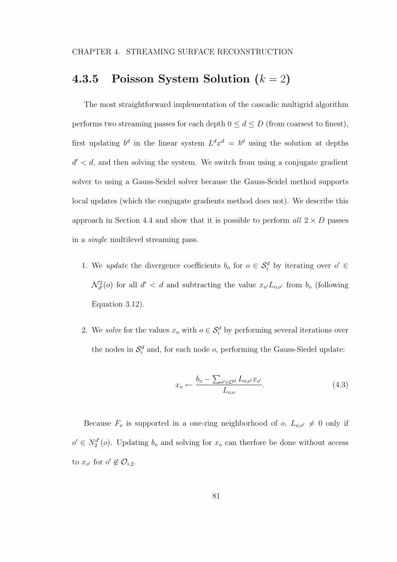
CHAPTER 4. STREAMING SURFACE RECONSTRUCTION
4.3.5 Poisson System Solution (k = 2)
The most straightforward implementation of the cascadic multigrid algorithm
performs two streaming passes for each depth 0 ≤ d ≤ D (from coarsest to finest),
first updating bd in the linear system Ldxd = bd using the solution at depths
d′ < d, and then solving the system. We switch from using a conjugate gradient
solver to using a Gauss-Seidel solver because the Gauss-Seidel method supports
local updates (which the conjugate gradients method does not). We describe this
approach in Section 4.4 and show that it is possible to perform all 2 ×D passes
in a single multilevel streaming pass.
1. We update the divergence coefficients bo for o ∈ Sdi by iterating over o′ ∈
N 2d′(o) for all d′ < d and subtracting the value xo′Lo,o′ from bo (following
Equation 3.12).
2. We solve for the values xo with o ∈ Sdi by performing several iterations over
the nodes in Sdi and, for each node o, performing the Gauss-Siedel update:
xo ←bo −
∑o′∈Od Lo,o′xo′
Lo,o
. (4.3)
Because Fo is supported in a one-ring neighborhood of o, Lo,o′ 6= 0 only if
o′ ∈ Nd′2 (o). Updating bo and solving for xo can therfore be done without access
to xo′ for o′ 6∈ Oi,2.
81
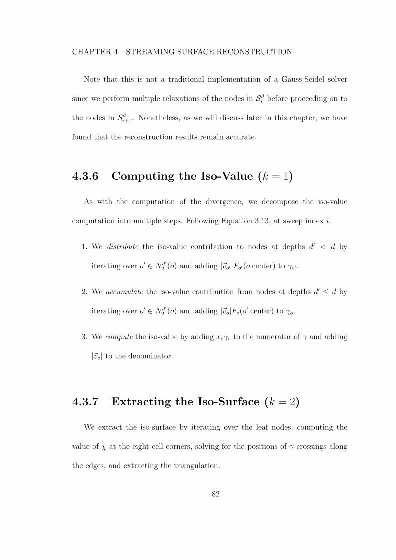
CHAPTER 4. STREAMING SURFACE RECONSTRUCTION
Note that this is not a traditional implementation of a Gauss-Seidel solver
since we perform multiple relaxations of the nodes in Sdi before proceeding on to
the nodes in Sdi+1. Nonetheless, as we will discuss later in this chapter, we have
found that the reconstruction results remain accurate.
4.3.6 Computing the Iso-Value (k = 1)
As with the computation of the divergence, we decompose the iso-value
computation into multiple steps. Following Equation 3.13, at sweep index i:
1. We distribute the iso-value contribution to nodes at depths d′ < d by
iterating over o′ ∈ Nd′2 (o) and adding |~vo′|Fo′(o.center) to γo′ .
2. We accumulate the iso-value contribution from nodes at depths d′ ≤ d by
iterating over o′ ∈ Nd′2 (o) and adding |~vo|Fo(o
′.center) to γo.
3. We compute the iso-value by adding xoγo to the numerator of γ and adding
|~vo| to the denominator.
4.3.7 Extracting the Iso-Surface (k = 2)
We extract the iso-surface by iterating over the leaf nodes, computing the
value of χ at the eight cell corners, solving for the positions of γ-crossings along
the edges, and extracting the triangulation.
82
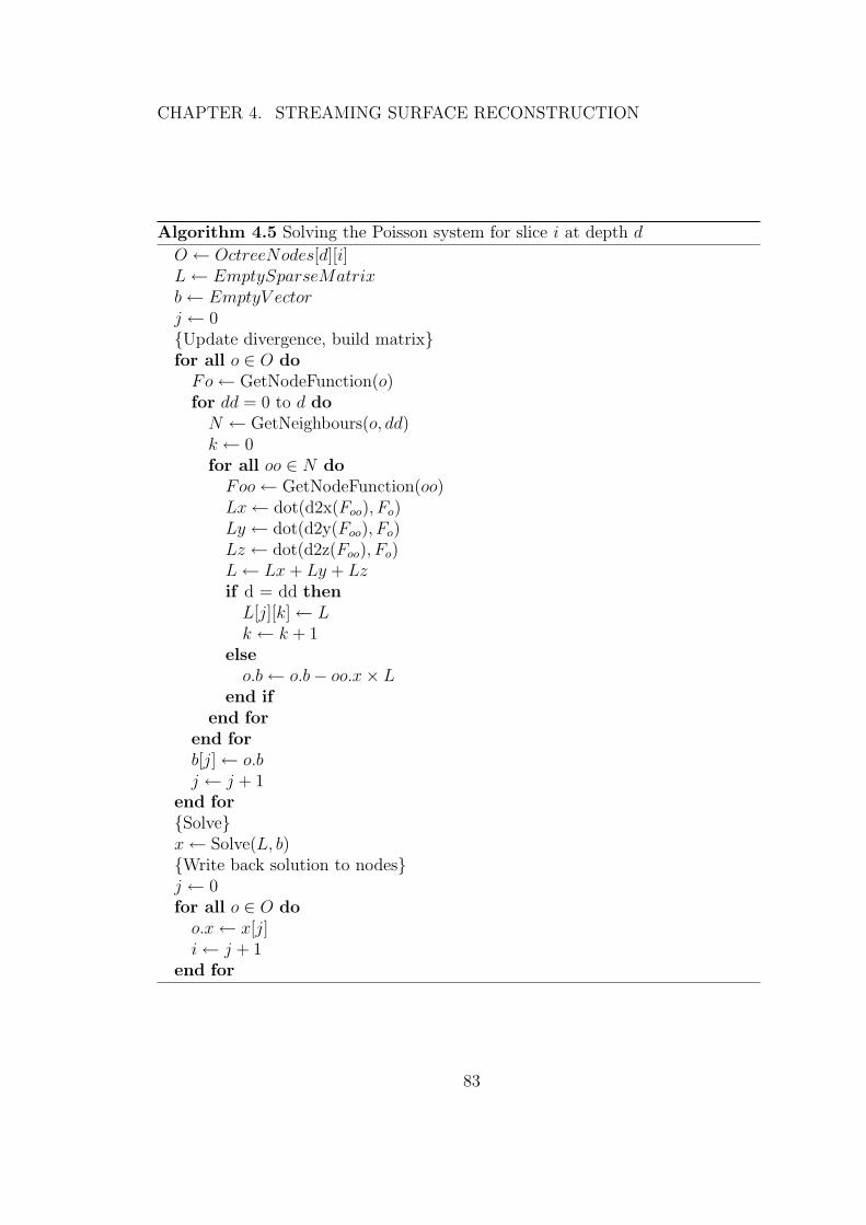
CHAPTER 4. STREAMING SURFACE RECONSTRUCTION
Algorithm 4.5 Solving the Poisson system for slice i at depth d
O ← OctreeNodes[d][i]L← EmptySparseMatrixb← EmptyV ectorj ← 0{Update divergence, build matrix}for all o ∈ O do
Fo← GetNodeFunction(o)for dd = 0 to d do
N ← GetNeighbours(o, dd)k ← 0for all oo ∈ N do
Foo← GetNodeFunction(oo)Lx← dot(d2x(Foo), Fo)Ly ← dot(d2y(Foo), Fo)Lz ← dot(d2z(Foo), Fo)L← Lx + Ly + Lzif d = dd then
L[j][k]← Lk ← k + 1
elseo.b← o.b− oo.x× L
end ifend for
end forb[j]← o.bj ← j + 1
end for{Solve}x← Solve(L, b){Write back solution to nodes}j ← 0for all o ∈ O do
o.x← x[j]i← j + 1
end for
83
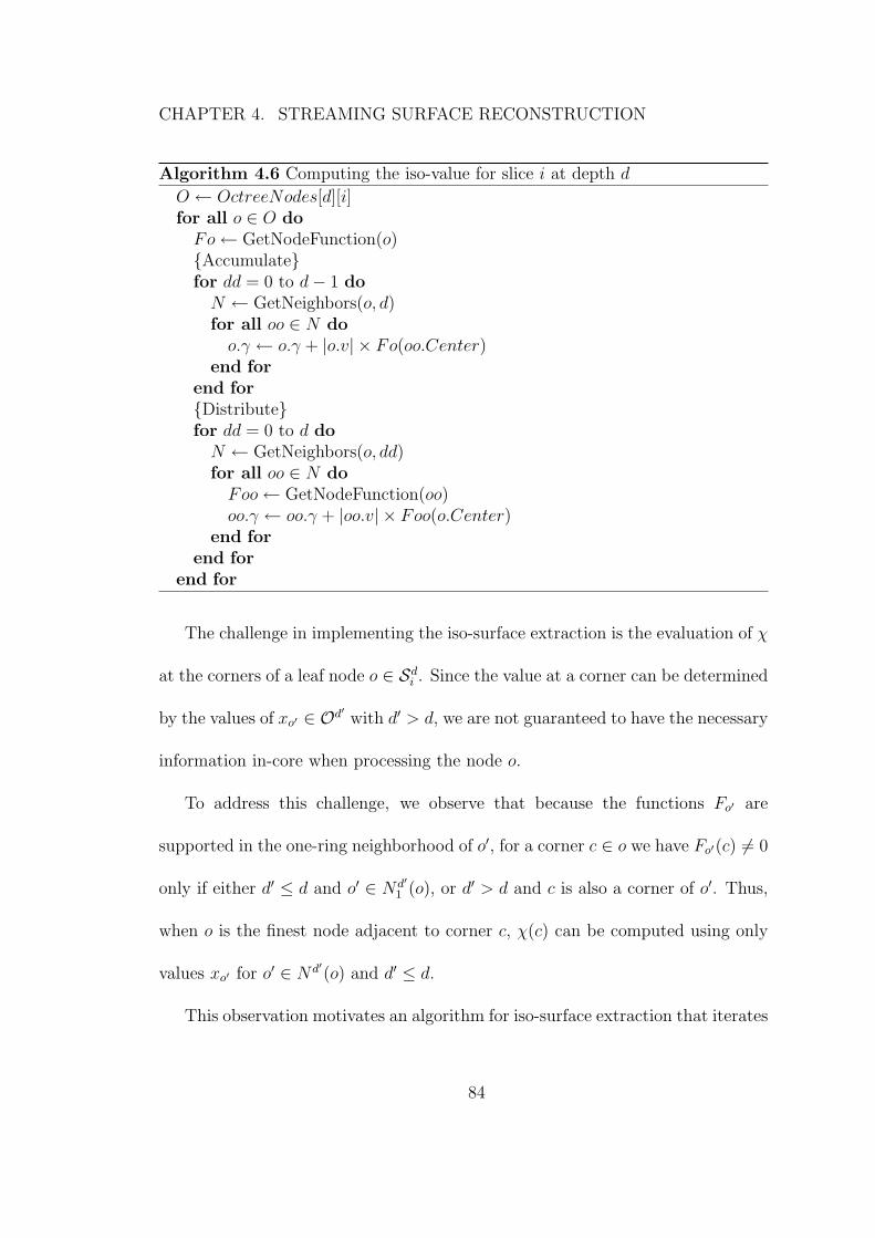
CHAPTER 4. STREAMING SURFACE RECONSTRUCTION
Algorithm 4.6 Computing the iso-value for slice i at depth d
O ← OctreeNodes[d][i]for all o ∈ O do
Fo← GetNodeFunction(o){Accumulate}for dd = 0 to d− 1 do
N ← GetNeighbors(o, d)for all oo ∈ N do
o.γ ← o.γ + |o.v| × Fo(oo.Center)end for
end for{Distribute}for dd = 0 to d do
N ← GetNeighbors(o, dd)for all oo ∈ N do
Foo← GetNodeFunction(oo)oo.γ ← oo.γ + |oo.v| × Foo(o.Center)
end forend for
end for
The challenge in implementing the iso-surface extraction is the evaluation of χ
at the corners of a leaf node o ∈ Sdi . Since the value at a corner can be determined
by the values of xo′ ∈ Od′with d′ > d, we are not guaranteed to have the necessary
information in-core when processing the node o.
To address this challenge, we observe that because the functions Fo′ are
supported in the one-ring neighborhood of o′, for a corner c ∈ o we have Fo′(c) 6= 0
only if either d′ ≤ d and o′ ∈ Nd′1 (o), or d′ > d and c is also a corner of o′. Thus,
when o is the finest node adjacent to corner c, χ(c) can be computed using only
values xo′ for o′ ∈ Nd′(o) and d′ ≤ d.
This observation motivates an algorithm for iso-surface extraction that iterates
84
CHAPTER 4. STREAMING SURFACE RECONSTRUCTION
over the leaf nodes, from the finest to the coarsest, and stores the evaluation of
χ at the corners in a temporary hash table. For a given corner c of a leaf node
o ∈ Od, we check if there is an entry in the hash table corresponding to c. If
there is not, this implies that there are no nodes at depth d′ > d containing c as a
corner and that the value χ(c) can be computed using only information associated
to nodes in the one-ring neighborhood of the ancestors of node o.
In practice, separate hash tables are associated with the corners of the front
and back of the leaf nodes at each depth. As the sweep plane is advanced, the front
hash table is updated by evaluating the front corners of leaf nodes intersecting
the sweep plane and the back corners of leaf nodes immediately in front of the
sweep plane. For a corner c ∈ o that is also a corner of a node o′ ∈ Od−1, we add
the value χ(c) to the front hash table at depth d− 1. Finally, after extracting the
iso-surface in the current sweep index, we swap the front and back hash tables
and clear the front one. It is also at this point that vertices are finalized [27].
To allow for efficient out-of-core rendering of our mesh, we write to a block-
based streaming mesh format. Unlike the approach of Isenburg et al. [27] we
separate the vertex data and triangle indices into two separate streams, which
store data in blocks of size b. To facilitate the efficient loading and unloading of
data, we also write an index structure that, for each block of triangles, references
the earliest and latest blocks of vertex data that are needed to be able to follow all
vertex indicies in the block. The earliest and latest vertex block indicies are then
85
CHAPTER 4. STREAMING SURFACE RECONSTRUCTION
optimized for streaming by making them monotonically increasing, making the
sequence of required vertex data blocks contiguous and always streaming forward
through the data. This index structure makes the process of streaming the mesh
for rendering or post-processing highly efficient. All loading and unloading of
vertex data is controlled by the index, alleviating the need to scan each triangle
as it is processed and maintain fine-grained book-keeping information.
4.4 An Optimized Implementation
In the previous section, we showed that the locality of the Poisson
reconstruction steps allows for stream processing. In this section, we show how
the different streaming passes can be merged into three multilevel streaming
passes. Our approach is motivated by two observations. First, we can merge
streaming steps when there are no conflicting data dependencies. Second, even
when there are dependencies, we may be able to pipeline the steps, resolving
the dependencies with only a small increase in the size of the working set. Due
to the data dependencies, three passes are a lower-bound for our reconstruction
algorithm:
• First Pass: We construct the octree, sample the weighting function, and
the vector field, and perform the distributive half of the divergence and
iso-value weighting calculations.
86
CHAPTER 4. STREAMING SURFACE RECONSTRUCTION
• Second Pass We perform the accumulative half of the divergence and
iso-value weighting calculations. Then, for each depth, we perform the
divergence update, construct and solve the Poisson system solution. Finally,
we compute the iso-value.
• Third Pass: We extract the iso-surface.
Because the values of {bo} for coarse nodes are not finalized until late in the
first pass, and because the linear systems at coarser depths need to be solved before
the systems at finer depths, the solving of the Poisson equation cannot begin until
the first pass has completed. This reflects the global nature of the Poisson system,
which requires all the data to have been seen before the solving can commence.
Similarly, the iso-surface extraction cannot being until the iso-value has been
computed, which is not complete until the solution has been completely solved.
4.4.1 First Pass (k = 6)
To merge the processing steps in the first pass, we must resolve the data
dependencies between different steps. We do this by pipelining the steps, delaying
execution of later steps to allow earlier steps to finalize the dependent data.
Using the sizes of the read/write neighborhoods described in Table 4.1, we can
resolve the data dependencies in the first pass by iterating over the sweep indices,
for each i:
87
CHAPTER 4. STREAMING SURFACE RECONSTRUCTION
• Constructing the octree for SD−1[i + 5]
and for each d ∈ Di
• Constructing the vector field for Sd[φd(i)]
• Distributing the divergence for Sd[φd(i)− 3]
• Distributing the iso-value contribution for Sd[φd(i)− 3]
Taking into account the size of the write neighborhoods for octree construction
and divergence distribution, the first pass of streaming reconstruction can be
implemented by maintaining the octree Oi,6 in the working set at sweep index i.
4.4.1.1 Buffering Samples
In addition to maintaining a small working octree, our method must also
address the fact that, to implement the vector field construction for block Sdi ,
the processing step needs access to each sample which lies in the span of Sdi and
has failed the density test at greater depths.
The exhaustive testing of all samples which lie in the span of Sdi can be a
computational bottleneck for our system since it requires D passes through the
ordered point set. This is unnecessarily expensive since we expect a sample’s
density estimate to increase by a factor of four as the depth is decremented. The
number of samples processed at depth d, but failing the density test, should drop
by a factor of four, while the number of samples that lie in the span of Sd−1i should
only increase by a factor of two.
88
CHAPTER 4. STREAMING SURFACE RECONSTRUCTION
We address this concern by associating a sample buffer to each depth and
processing the blocks in decreasing depth order. Samples are added into the
buffer at depth D during the octree construction step, and are promoted to the
buffer at depth d − 1 if they fail the density test at depth d in the vector field
construction step. (Points in the depth-d buffer that lie in the span of Sd[φd(i)]
are removed from the buffer at the end of the vector field construction step.)
4.4.2 Second Pass (k = 8)
As in the first pass, we merge the steps in the second pass by pipelining them
to resolve data dependencies. However, since the consolidation of these steps into
a single pass forces us to iterate over the depths before iterating over the sweep
indices, the merging of the divergence update with the Poisson system solution
poses a challenge. For a fixed sweep index, we can no longer treat the individual
steps as atomic because this would result in a circular data dependency: the
modification of {bo} in the divergence update requires access to {xo} set in the
Poisson system solver which, in turn, requires access to {bo}.
We resolve this problem by separately considering the pipelining that needs
to be performed to resolve the data dependencies due to sweep index and due to
depth.
89
CHAPTER 4. STREAMING SURFACE RECONSTRUCTION
4.4.2.1 Index Dependencies
Fixing a depth d and assuming no cross-depth data dependencies, we define
the scheduling as we did in the first pass. Iterating over the (depth-relative) sweep
index id, with 0 ≤ id < 2d, we:
• Accumulate the iso-value contribution for Sd[id]
• Accumulate the divergence for Sd[id]
• Update the divergence for Sd[id]
• Solve the Poisson system for Sd[id − 3]
• Compute the iso-value for Sd[id − 4]
4.4.2.2 Depth Dependencies
To resolve the depth-related dependencies, we offset the values of id so that
values required at finer depths are guaranteed to have been set at coarser ones.
Analyzing the size of the read/write neighborhoods shows that the
dependencies can be resolved if the indices satisfy the property id−1 ≥ bid/2c+ 6.
Expressing id as an offset from the finest index, id = φd(ih−1) + δd, and
initializing with δh−1 = 0, we obtain a recursive expression for the offsets:
~δd = {11, . . . , 11, 10, 9, 6, 0}. Thus, setting ih−1 = i− 3, the second reconstruction
pass can be implemented by maintaining the octree Oi,8 in the working set at
sweep index i.
In practice, we can further reduce the memory requirements by observing that
90
CHAPTER 4. STREAMING SURFACE RECONSTRUCTION
processing at the finest depths requires a narrower window size. This allows us to
maintain a working octree with fewer stream blocks at the finest depths.
Figure 4.1 shows an example of the three streaming passes for the
reconstruction of a 2D point set, showing the state of the reconstruction at
different sweep indices (indicated by the arrows). As can be seen, the offsetting
of the pipeline steps in the second pass forces coarser nodes to be solved ahead
of the sweep line, resulting in a lower resolution reconstruction emerging to the
right of the sweep index.
4.5 Results
4.5.1 Large Datasets
To evaluate our method, we have reconstructed highly detailed surfaces from
large scanned datasets, as summarized in Table 4.2. All results use a target of
κ = 2 samples per octree node. Figure 4.6 shows a surface reconstruction of
Michelangelo’s David statue from an input of 216M oriented points from raw
scan data. The output surface of 210M triangles was generated at depth 13, and
required only 780 MB of memory. In contrast, the in-core algorithm presented in
Chapter 3 only produced a 20M triangle approximation of this same model (at
depth 11), and required 4.4 GB of memory. Figure 4.5 shows a close-up visual
comparison.
91
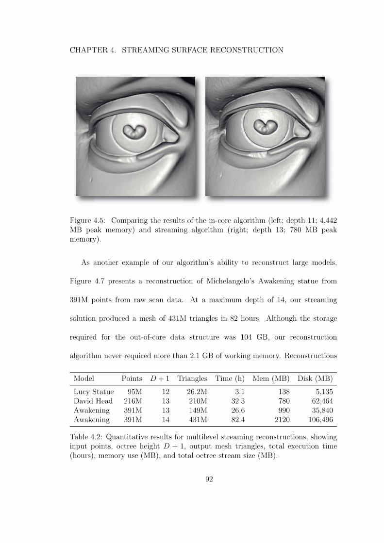
CHAPTER 4. STREAMING SURFACE RECONSTRUCTION
Figure 4.5: Comparing the results of the in-core algorithm (left; depth 11; 4,442MB peak memory) and streaming algorithm (right; depth 13; 780 MB peakmemory).
As another example of our algorithm’s ability to reconstruct large models,
Figure 4.7 presents a reconstruction of Michelangelo’s Awakening statue from
391M points from raw scan data. At a maximum depth of 14, our streaming
solution produced a mesh of 431M triangles in 82 hours. Although the storage
required for the out-of-core data structure was 104 GB, our reconstruction
algorithm never required more than 2.1 GB of working memory. Reconstructions
Model Points D + 1 Triangles Time (h) Mem (MB) Disk (MB)
Lucy Statue 95M 12 26.2M 3.1 138 5,135David Head 216M 13 210M 32.3 780 62,464Awakening 391M 13 149M 26.6 990 35,840Awakening 391M 14 431M 82.4 2120 106,496
Table 4.2: Quantitative results for multilevel streaming reconstructions, showinginput points, octree height D + 1, output mesh triangles, total execution time(hours), memory use (MB), and total octree stream size (MB).
92
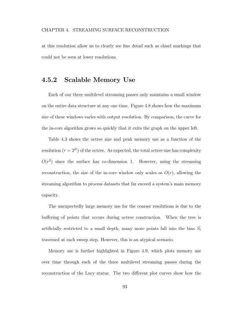
CHAPTER 4. STREAMING SURFACE RECONSTRUCTION
at this resolution allow us to clearly see fine detail such as chisel markings that
could not be seen at lower resolutions.
4.5.2 Scalable Memory Use
Each of our three multilevel streaming passes only maintains a small window
on the entire data structure at any one time. Figure 4.8 shows how the maximum
size of these windows varies with output resolution. By comparison, the curve for
the in-core algorithm grows so quickly that it exits the graph on the upper left.
Table 4.3 shows the octree size and peak memory use as a function of the
resolution (r = 2D) of the octree. As expected, the total octree size has complexity
O(r2) since the surface has co-dimension 1. However, using the streaming
reconstruction, the size of the in-core window only scales as O(r), allowing the
streaming algorithm to process datasets that far exceed a system’s main memory
capacity.
The unexpectedly large memory use for the coarser resolutions is due to the
buffering of points that occurs during octree construction. When the tree is
artificially restricted to a small depth, many more points fall into the bins Si
traversed at each sweep step. However, this is an atypical scenario.
Memory use is further highlighted in Figure 4.9, which plots memory use
over time through each of the three multilevel streaming passes during the
reconstruction of the Lucy statue. The two different plot curves show how the
93
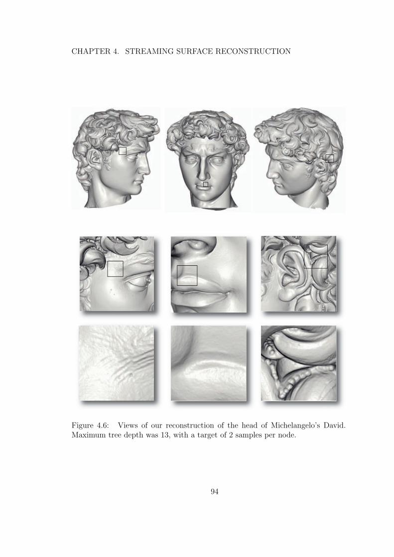
CHAPTER 4. STREAMING SURFACE RECONSTRUCTION
Figure 4.6: Views of our reconstruction of the head of Michelangelo’s David.Maximum tree depth was 13, with a target of 2 samples per node.
94
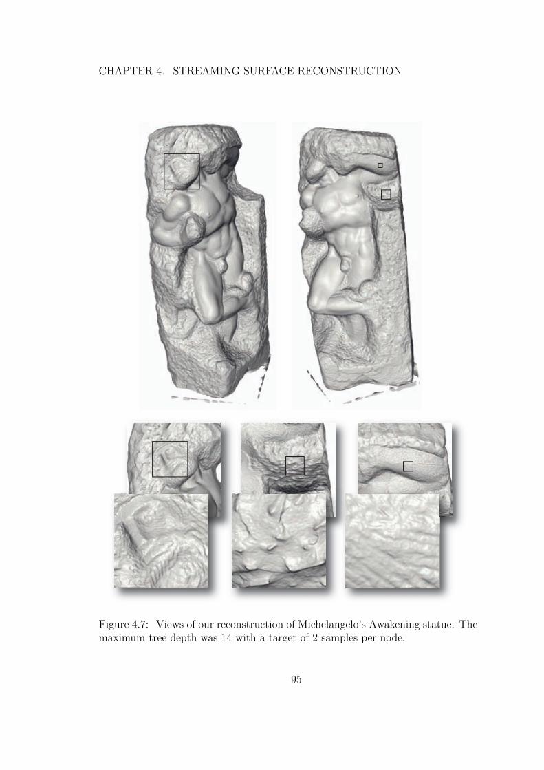
CHAPTER 4. STREAMING SURFACE RECONSTRUCTION
Figure 4.7: Views of our reconstruction of Michelangelo’s Awakening statue. Themaximum tree depth was 14 with a target of 2 samples per node.
95
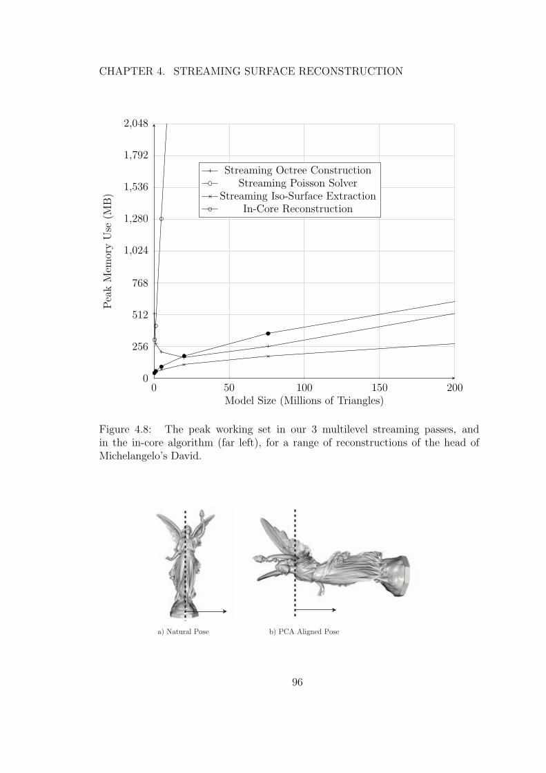
CHAPTER 4. STREAMING SURFACE RECONSTRUCTION
0 50 100 150 2000
256
512
768
1,024
1,280
1,536
1,792
2,048
Model Size (Millions of Triangles)
Pea
kM
emor
yU
se(M
B)
Streaming Octree ConstructionStreaming Poisson Solver
Streaming Iso-Surface ExtractionIn-Core Reconstruction
Figure 4.8: The peak working set in our 3 multilevel streaming passes, andin the in-core algorithm (far left), for a range of reconstructions of the head ofMichelangelo’s David.
a) Natural Pose b) PCA Aligned Pose
96
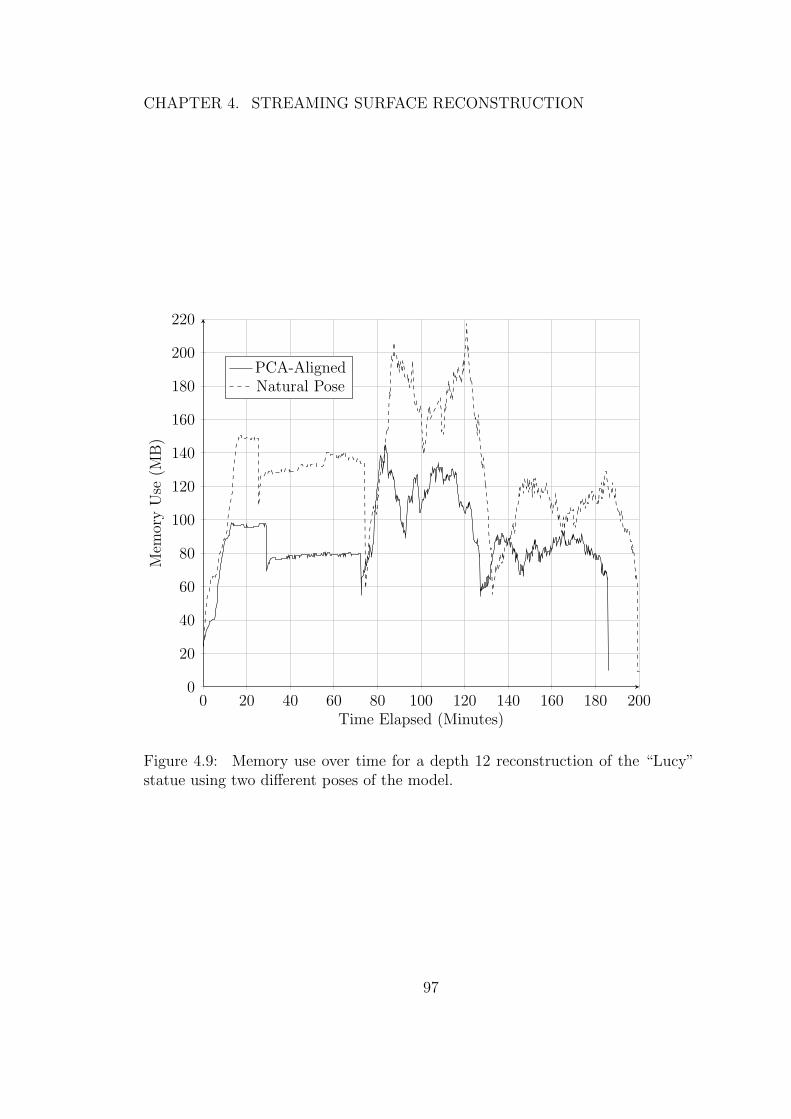
CHAPTER 4. STREAMING SURFACE RECONSTRUCTION
0 20 40 60 80 100 120 140 160 180 2000
20
40
60
80
100
120
140
160
180
200
220
Time Elapsed (Minutes)
Mem
ory
Use
(MB
)
PCA-AlignedNatural Pose
Figure 4.9: Memory use over time for a depth 12 reconstruction of the “Lucy”statue using two different poses of the model.
97
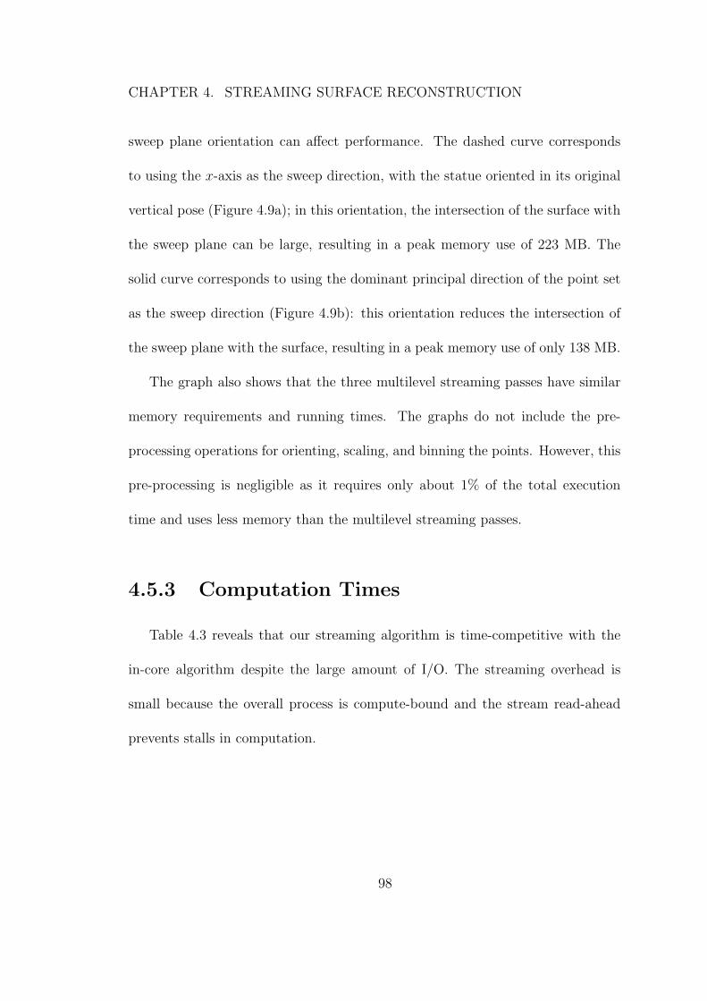
CHAPTER 4. STREAMING SURFACE RECONSTRUCTION
sweep plane orientation can affect performance. The dashed curve corresponds
to using the x-axis as the sweep direction, with the statue oriented in its original
vertical pose (Figure 4.9a); in this orientation, the intersection of the surface with
the sweep plane can be large, resulting in a peak memory use of 223 MB. The
solid curve corresponds to using the dominant principal direction of the point set
as the sweep direction (Figure 4.9b): this orientation reduces the intersection of
the sweep plane with the surface, resulting in a peak memory use of only 138 MB.
The graph also shows that the three multilevel streaming passes have similar
memory requirements and running times. The graphs do not include the pre-
processing operations for orienting, scaling, and binning the points. However, this
pre-processing is negligible as it requires only about 1% of the total execution
time and uses less memory than the multilevel streaming passes.
4.5.3 Computation Times
Table 4.3 reveals that our streaming algorithm is time-competitive with the
in-core algorithm despite the large amount of I/O. The streaming overhead is
small because the overall process is compute-bound and the stream read-ahead
prevents stalls in computation.
98
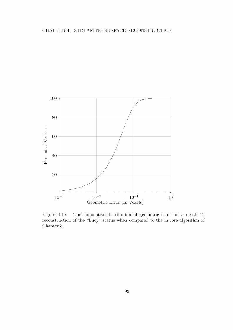
CHAPTER 4. STREAMING SURFACE RECONSTRUCTION
10−3 10−2 10−1 100
20
40
60
80
100
Geometric Error (In Voxels)
Per
cent
ofV
erti
ces
Figure 4.10: The cumulative distribution of geometric error for a depth 12reconstruction of the “Lucy” statue when compared to the in-core algorithm ofChapter 3.
99
CHAPTER 4. STREAMING SURFACE RECONSTRUCTION
4.5.4 Streaming Solver Accuracy
Because our streaming solver computes an iterative solution to the Poisson
equation, the numerical accuracy of the solution could impact the geometric
accuracy of the resulting surface mesh. (This topic is discussed further in
Section 4.6.) To test geometric accuracy, we compare the surface mesh generated
by our streaming algorithm to that generated by the in-core algorithm presented in
Chapter 3. Figure 4.10 graphs the cumulative distribution of reconstruction error,
measured as the distance in voxel units from vertices on the reconstructed surface
to the nearest points on the reference surface. Despite the fact that our streaming
cascadic multigrid performs only a single sweep at each level, the resulting surface
mesh is still very accurate – only 8% of the vertices have an error greater than 0.1
voxels, and the maximum error is 0.651 voxels.
4.6 Discussion
Solving the Poisson system in streaming fashion is a challenging task since it
involves a global linear system in which Laplacian values at one point affect the
solution at points faraway. The key ingredient that enables an effective streaming
solution is the use of a cascading multigrid approach.
To demonstrate the importance of a multi-grid solver, Figure 4.11 shows the
quality of solutions to a 2D Poisson problem using three different techniques. The
100
CHAPTER 4. STREAMING SURFACE RECONSTRUCTION
first row shows the reconstructions obtained with 1, 4, 16, and 64 iterations of a
Gauss-Seidel solver that streams through the column blocks of the image, much
like one of the single-level streaming passes described in Section 4.4. As shown in
the second row, even if we replace the Gauss-Seidel solver with the more efficient
(but non-streaming) conjugate-gradient solver, the convergence is still too slow,
requiring at least 64 passes through the data to obtain an approximate solution.
In contrast, a cascadic multigrid solver (bottom row) quickly converges to the
indicator function.
For general problems, a multigrid solver typically requires V-cycles, which
could involve more streaming passes, but remarkably, for our reconstruction
problem, a single cascadic pass is usually sufficient. The intuition is that, in
the context of surface reconstruction, the Poisson solution χ approximates an
indicator function, and is thus only used to identify the boundary between the
interior and exterior of an object.
Because the indicator function is a binary function whose value is either 0 or 1,
and the iso-value is approximately 0.5, the reconstruction is sufficiently accurate
if it never differs by more than 0.5 from the indicator function. As shown in the
bottom left reconstruction of Figure 4.11 (and also earlier in Figure 4.10), this
relaxed error condition can be met with just one iteration per level of the cascadic
multigrid solver, allowing us to perform a single streaming pass at each level. And,
one of our key algorithmic contributions is to show that all such passes can be
101

CHAPTER 4. STREAMING SURFACE RECONSTRUCTION
combined into a single multilevel streaming pass.
102
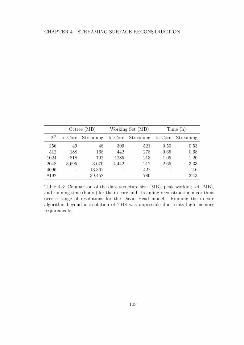
CHAPTER 4. STREAMING SURFACE RECONSTRUCTION
Octree (MB) Working Set (MB) Time (h)
2D In-Core Streaming In-Core Streaming In-Core Streaming
256 49 48 309 521 0.50 0.53512 188 168 442 278 0.65 0.68
1024 818 702 1285 213 1.05 1.202048 3,695 3,070 4,442 212 2.65 3.334096 - 13,367 - 427 - 12.68192 - 39,452 - 780 - 32.3
Table 4.3: Comparison of the data structure size (MB), peak working set (MB),and running time (hours) for the in-core and streaming reconstruction algorithmsover a range of resolutions for the David Head model. Running the in-corealgorithm beyond a resolution of 2048 was impossible due to its high memoryrequirements.
103
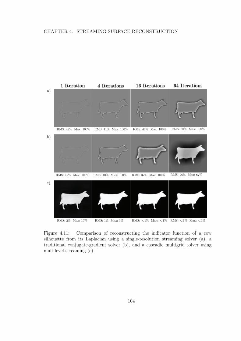
CHAPTER 4. STREAMING SURFACE RECONSTRUCTION
1 Iteration 4 Iterations 16 Iterations 64 Iterations
RMS: 42% Max: 100% RMS: 41% Max: 100% RMS: 40% Max: 100% RMS: 38% Max: 100%
RMS: 42% Max: 100% RMS: 40% Max: 100% RMS: 37% Max: 100% RMS: 26% Max: 67%
RMS: 2% Max: 19% RMS: 1% Max: 3% RMS: <1% Max: <1% RMS: <1% Max: <1%
a)
b)
c)
Figure 4.11: Comparison of reconstructing the indicator function of a cowsilhouette from its Laplacian using a single-resolution streaming solver (a), atraditional conjugate-gradient solver (b), and a cascadic multigrid solver usingmultilevel streaming (c).
104
Chapter 5
Parallel Surface Reconstruction
In Chapter 4, we were able to express all the computation steps of the Poisson
Surface Reconstruction algorithm as local updates. This locality of data reference
permitted the reconstruction to be performed as a set of streaming operations,
significantly reducing the main memory required to reconstruct extremely large
datasets: the reconstruction of Michelangelo’s Awakening from 391 million data
points only required 2120 megabytes of working memory. Although the streaming
technique makes it possible to reconstruct large models on a commodity computer,
the processing time is still significant: the reconstruction of Awakening required
82 hours of processor time. As datasets increase in size, the processing time could
grow to weeks or months.
To address these practical limitations, we take advantage of the recent
trend in microprocessor evolution toward parallelism. Multi-core processors are
105
CHAPTER 5. PARALLEL SURFACE RECONSTRUCTION
now commonplace among commodity computers, and highly parallel graphics
hardware provides even higher performance per watt. Traditional single-threaded
algorithms will no longer benefit from Moore’s law, introducing a new age in
computer science in which efficient parallel implementations are required.
This chapter presents an efficient, scalable, parallel implementation of the
Poisson Surface Reconstruction algorithm. The system is designed to run on
modern parallel computer systems, allowing the reconstruction of some of the
largest available datasets in significantly less time than previously possible. We
begin by describing a parallel implementation designed for multi-core systems with
shared memory (i.e. processors sharing a common main memory). We show that,
although simple to implement and effective on dual-core processors, this model
ultimately lacks the scalability required for large problems. Analyzing the shared-
memory implementation provides valuable insight regarding the key properties a
parallel solver must satisfy to demonstrate good speed-up when parallelized across
numerous processors. We then describe a design based on a distributed memory
model. The elimination of frequent data sharing and synchronization allows the
distributed system to scale to twelve processors across multiple machines.
106
CHAPTER 5. PARALLEL SURFACE RECONSTRUCTION
5.1 Related Work
Despite the increasing presence of commodity parallel computing systems,
there has been comparatively little work on parallel surface reconstruction. Some
surface reconstruction algorithms naturally lend themselves to efficient parallel
implementations.
Many local implicit function fitting methods can be at least partially
parallelized by virtue of the locality of most data dependencies. For example,
the VRIP [17] method can partition the voxel grid across a number of processors.
With an appropriate padding region, all data dependencies become local and each
processor is able to independently construct the distance function and extract the
triangles for a portion of surface. Surface patches can then be zippered together
to form a complete model.
Global implicit function fitting methods often have complex data dependencies
that inhibit parallelism. One notable exception to this is the FFT method [31],
which can be efficiently computed in parallel by virtue of extensive use of Fast
Fourier Transforms, which have well known parallel implementations on a variety
of platforms [1, 40].
Computational geometry approaches can leverage parallel processing by
computing structures such as the Delaunay triangulation in parallel (e.g. [24]).
The work of [59] implements our Poisson method on the GPU, achieving
significant speedups for small datasets. A limitation of the implementation is that
107
CHAPTER 5. PARALLEL SURFACE RECONSTRUCTION
it requires the entire octree, dataset and supplemental lookup tables to reside in
GPU memory, limiting the maximum size of reconstructions possible. To simplify
the lookup of neighbor nodes in the octree and reduce the total number of node
computations required, the implementation also only uses first-order elements.
5.2 Parallel Reconstruction
When designing the streaming implementation, one of the primary concerns
was minimizing the effect of the I/O required for out-of-core processing. In
particular, this motivated the streaming approach (since streaming I/O is highly
efficient) and the minimization of the number of passes required through the data
(minimizing the total amount of I/O performed). When considering a parallel
implementation, a different set of design concerns prevail: minimizing data sharing
and synchronization.
5.3 Shared Memory
The most straightforward parallelization of the serial streaming implementa-
tion executes node kernel functions in parallel. Almost all of the total computation
time is spent executing node functions across the octree, and the restrictions
placed on node function data dependencies for efficient streaming allow the
functions within a slice to be executed in any order. With slices in large
108
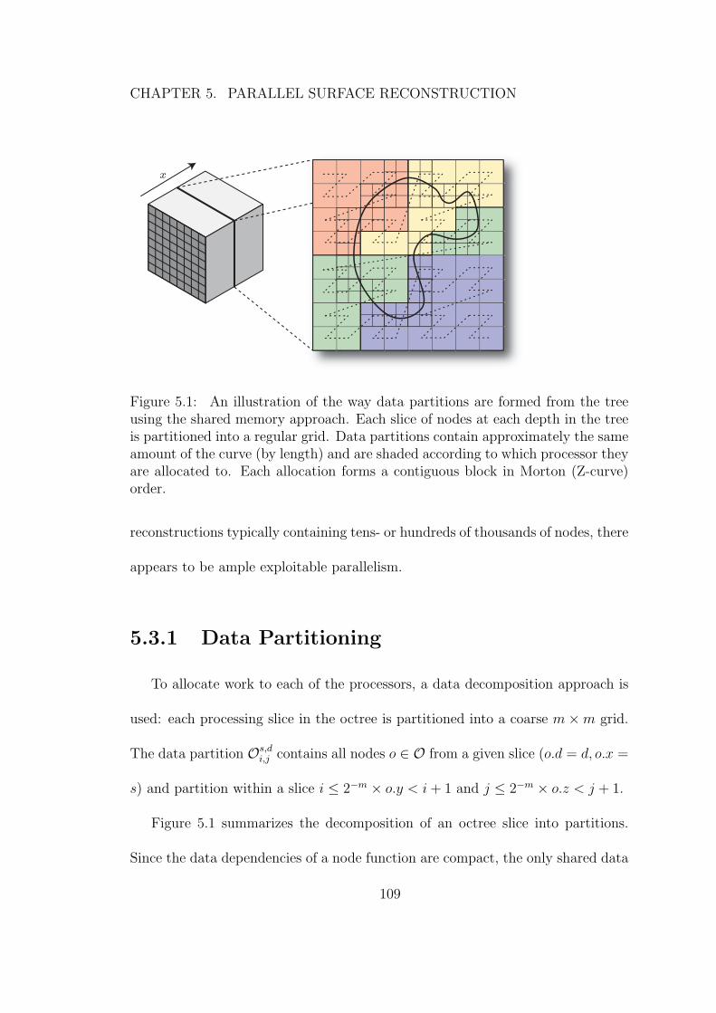
CHAPTER 5. PARALLEL SURFACE RECONSTRUCTION
x
Figure 5.1: An illustration of the way data partitions are formed from the treeusing the shared memory approach. Each slice of nodes at each depth in the treeis partitioned into a regular grid. Data partitions contain approximately the sameamount of the curve (by length) and are shaded according to which processor theyare allocated to. Each allocation forms a contiguous block in Morton (Z-curve)order.
reconstructions typically containing tens- or hundreds of thousands of nodes, there
appears to be ample exploitable parallelism.
5.3.1 Data Partitioning
To allocate work to each of the processors, a data decomposition approach is
used: each processing slice in the octree is partitioned into a coarse m×m grid.
The data partition Os,di,j contains all nodes o ∈ O from a given slice (o.d = d, o.x =
s) and partition within a slice i ≤ 2−m × o.y < i + 1 and j ≤ 2−m × o.z < j + 1.
Figure 5.1 summarizes the decomposition of an octree slice into partitions.
Since the data dependencies of a node function are compact, the only shared data
109
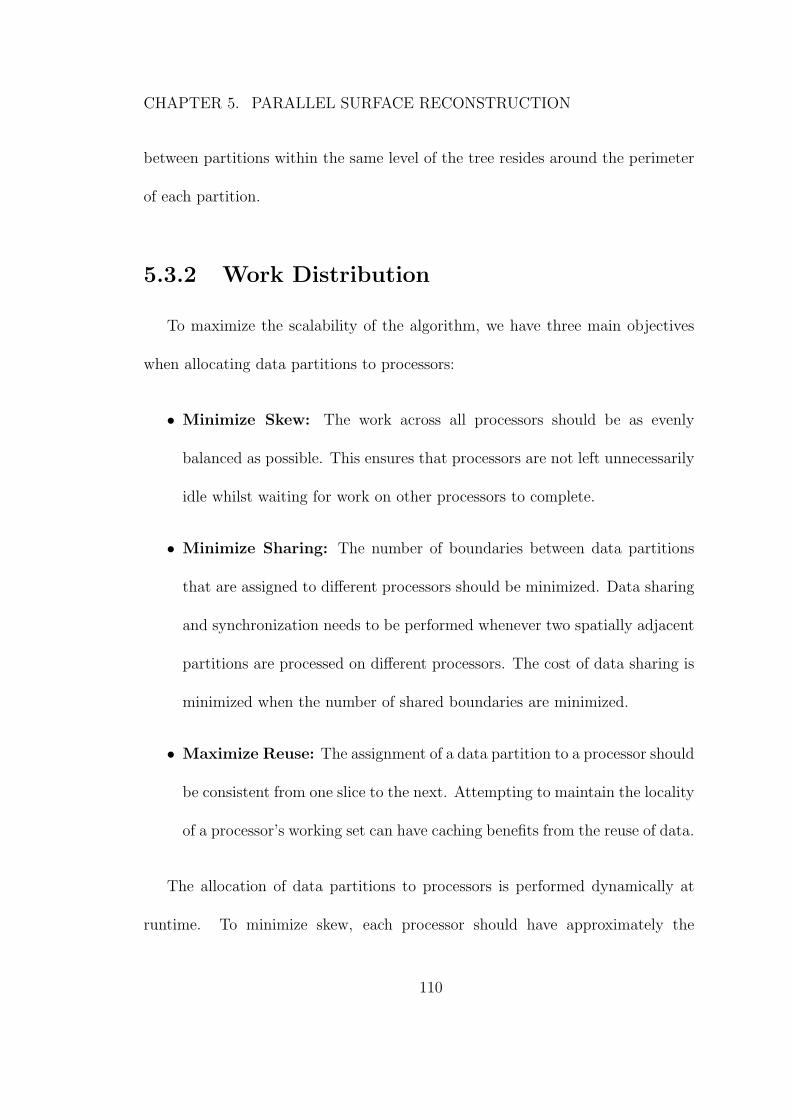
CHAPTER 5. PARALLEL SURFACE RECONSTRUCTION
between partitions within the same level of the tree resides around the perimeter
of each partition.
5.3.2 Work Distribution
To maximize the scalability of the algorithm, we have three main objectives
when allocating data partitions to processors:
• Minimize Skew: The work across all processors should be as evenly
balanced as possible. This ensures that processors are not left unnecessarily
idle whilst waiting for work on other processors to complete.
• Minimize Sharing: The number of boundaries between data partitions
that are assigned to different processors should be minimized. Data sharing
and synchronization needs to be performed whenever two spatially adjacent
partitions are processed on different processors. The cost of data sharing is
minimized when the number of shared boundaries are minimized.
• Maximize Reuse: The assignment of a data partition to a processor should
be consistent from one slice to the next. Attempting to maintain the locality
of a processor’s working set can have caching benefits from the reuse of data.
The allocation of data partitions to processors is performed dynamically at
runtime. To minimize skew, each processor should have approximately the
110
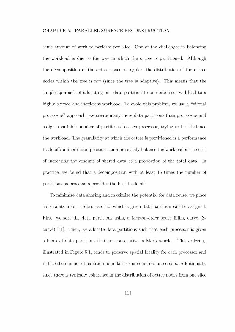
CHAPTER 5. PARALLEL SURFACE RECONSTRUCTION
same amount of work to perform per slice. One of the challenges in balancing
the workload is due to the way in which the octree is partitioned. Although
the decomposition of the octree space is regular, the distribution of the octree
nodes within the tree is not (since the tree is adaptive). This means that the
simple approach of allocating one data partition to one processor will lead to a
highly skewed and inefficient workload. To avoid this problem, we use a “virtual
processors” approach: we create many more data partitions than processors and
assign a variable number of partitions to each processor, trying to best balance
the workload. The granularity at which the octree is partitioned is a performance
trade-off: a finer decomposition can more evenly balance the workload at the cost
of increasing the amount of shared data as a proportion of the total data. In
practice, we found that a decomposition with at least 16 times the number of
partitions as processors provides the best trade off.
To minimize data sharing and maximize the potential for data reuse, we place
constraints upon the processor to which a given data partition can be assigned.
First, we sort the data partitions using a Morton-order space filling curve (Z-
curve) [41]. Then, we allocate data partitions such that each processor is given
a block of data partitions that are consecutive in Morton-order. This ordering,
illustrated in Figure 5.1, tends to preserve spatial locality for each processor and
reduce the number of partition boundaries shared across processors. Additionally,
since there is typically coherence in the distribution of octree nodes from one slice
111
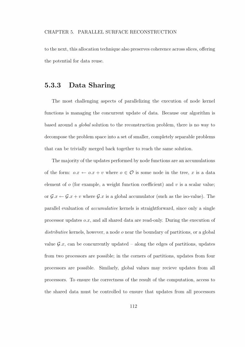
CHAPTER 5. PARALLEL SURFACE RECONSTRUCTION
to the next, this allocation technique also preserves coherence across slices, offering
the potential for data reuse.
5.3.3 Data Sharing
The most challenging aspects of parallelizing the execution of node kernel
functions is managing the concurrent update of data. Because our algorithm is
based around a global solution to the reconstruction problem, there is no way to
decompose the problem space into a set of smaller, completely separable problems
that can be trivially merged back together to reach the same solution.
The majority of the updates performed by node functions are an accumulations
of the form: o.x ← o.x + v where o ∈ O is some node in the tree, x is a data
element of o (for example, a weight function coefficient) and v is a scalar value;
or G.x← G.x + v where G.x is a global accumulator (such as the iso-value). The
parallel evaluation of accumulative kernels is straightforward, since only a single
processor updates o.x, and all shared data are read-only. During the execution of
distributive kernels, however, a node o near the boundary of partitions, or a global
value G.x, can be concurrently updated – along the edges of partitions, updates
from two processors are possible; in the corners of partitions, updates from four
processors are possible. Similarly, global values may recieve updates from all
processors. To ensure the correctness of the result of the computation, access to
the shared data must be controlled to ensure that updates from all processors
112
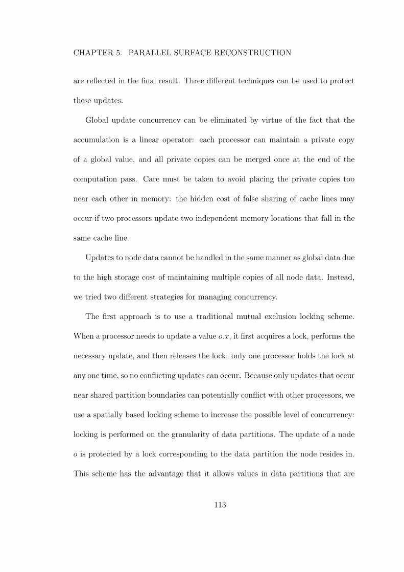
CHAPTER 5. PARALLEL SURFACE RECONSTRUCTION
are reflected in the final result. Three different techniques can be used to protect
these updates.
Global update concurrency can be eliminated by virtue of the fact that the
accumulation is a linear operator: each processor can maintain a private copy
of a global value, and all private copies can be merged once at the end of the
computation pass. Care must be taken to avoid placing the private copies too
near each other in memory: the hidden cost of false sharing of cache lines may
occur if two processors update two independent memory locations that fall in the
same cache line.
Updates to node data cannot be handled in the same manner as global data due
to the high storage cost of maintaining multiple copies of all node data. Instead,
we tried two different strategies for managing concurrency.
The first approach is to use a traditional mutual exclusion locking scheme.
When a processor needs to update a value o.x, it first acquires a lock, performs the
necessary update, and then releases the lock: only one processor holds the lock at
any one time, so no conflicting updates can occur. Because only updates that occur
near shared partition boundaries can potentially conflict with other processors, we
use a spatially based locking scheme to increase the possible level of concurrency:
locking is performed on the granularity of data partitions. The update of a node
o is protected by a lock corresponding to the data partition the node resides in.
This scheme has the advantage that it allows values in data partitions that are
113
CHAPTER 5. PARALLEL SURFACE RECONSTRUCTION
spatially separate from each other to be updated without interference. A further
optimization can be made for data partitions that are “interior” to a processor’s
work block: if a data partition does not share an edge or corner with a data
partition assigned to another processor, then no locking need occur since it is not
possible for another processor to need to update its values.
The second approach is to utilize the atomic compare and swap (CAS)
instruction found in many modern microprocessor architectures. Given a memory
address A, a comparison value c and a replacement value x, the processor then
performs the update A← x if and only if A = c, atomically (i.e. the comparison
and the assignment are performed as a single, uninterruptable sequence). This
instruction can be used to construct a lightweight, optimistic, floating-point
atomic accumulation function that can be used in our algorithm. The algorithm
is presented in Algorithm 5.1. The method works by recording the existing value
of c← A and optimistically updating A′ ← c+x. The CAS primitive is then used
to atomically test the current value of A and then attempt to update A ← A′
if the value of A is unchanged (i.e. no other update has occurred from another
processor). If the CAS operation fails, the procedure is repeated. The number
of update attempts will be proportional to the level of contention on the shared
data. Although this technique is vulnerable to the so-called “ABA” problem, such
a situation does not affect the correctness in our situation.
We implemented both of these approaches and present the results in Section 5.3.4.
114
CHAPTER 5. PARALLEL SURFACE RECONSTRUCTION
Algorithm 5.1 The lock-free accumulate operation for floating-point numbersrepeat
c← AA′ ← c + x
until CAS(A, c, A′) 6= c
In addition to the most common case of accumulating data in tree nodes or
global variables, there are two other types of concurrent updates in our method
that are worthy of further detail.
5.3.3.1 Tree Construction
In Section 4.3.2, we described the way in which tree nodes are created in an
in-core octree before the nodes are written to the out-of-core node streams. When
implementing this in a parallel setting, we partition the point set using the same
data partitioning scheme that is used for node data: for each slice of points,
we partition the slice into an m × m grid and partition the points according to
the block they fall into. Using this scheme, we can construct the in-core tree
in parallel by simultaneously constructing independent branches of the in-core
tree on different processors. One complication, however, is that to facilitate the
splatting of a point into the tree to create the approximation to the gradient of
the indicator function, we require the one-ring neighborhood of nodes around any
node which contains a point sample to exist in the tree. When points fall near
a partition boundary, this refinement step requires nodes to be created that fall
into a branch of the tree being constructed simultaneously on another processor.
115
CHAPTER 5. PARALLEL SURFACE RECONSTRUCTION
To prevent race conditions during the allocation and attachment of nodes to the
tree, we again use the atomic compare and swap instruction. The steps to create
a new tree node are presented in Algorithm 5.2. The technique uses the compare
and swap operation to set the child pointer of a tree node to a newly initialized
brood of nodes only if the child pointer is null.
Algorithm 5.2 The lock-free atomic operation for creating in-core tree nodes
if n.children = 0 thenn′ ← CreateNoden.children = CAS(n.children, 0, n′)if n.children 6= n′ then
DeleteNode(n′)end if
end if
5.3.3.2 Solving the Laplacian
Although the process of solving the linear system can be performed using our
concurrent update scheme from Section 5.3.3, we leverage some unique properties
of the solver to eliminate the need to perform synchronization and locking. In the
streaming implementation from Chapter 4, to solve the Laplacian at a given slice
and depth we construct a single linear system L~x = ~b and solve for ~x, the vector
of solution coefficients, using several iterations of Gauss-Siedel updates.
To solve this same problem in parallel, we construct separate linear systems per
processor and solve them independently. Each processor solves for (i.e. updates)
the portion of ~x whose nodes fall within its data partitions. To ensure that
116
CHAPTER 5. PARALLEL SURFACE RECONSTRUCTION
the solution propagates correctly across data partition boundaries, all processors
share a common ~x so that updates to solution values during solver iterations
are immediately visible to other processors. Note that although this causes
unsynchronized access to shared data, there are two characteristics of our Gauss-
Seidel solver that ensure the accuracy of the solution is maintained. First, the
write of a single solution value (i.e. a single 32-bit word of memory) is an atomic
operation: when other processors read the value, they will either see an old value,
or a new value, not a combination of the two. Second, the solver we are using
is resilient to reading older solution values, mixed with newer values. While
this could lead to a situation in which the subsequent relaxations of previously
relaxed coefficients near the partition boundary read un-relaxed values from their
neighbors, we have found that in practice this is not a problem.
5.3.4 Scalability Issues
Figure 5.2 presents the scalability of the shared memory implementation,
reconstructing the Lucy model at depth 12 from one to eight cores. The processor
cores were arranged in a 2x2x2 configuration: 2 cores per die, 2 dies per package,
with 2 sockets in the machine. Each core has a private 32KB L1 data cache and
each die shares a 6MB L2 data cache. Although the shared memory approach
provides a straightforward implementation, in practice it was found to have two
significant scalability issues.
117
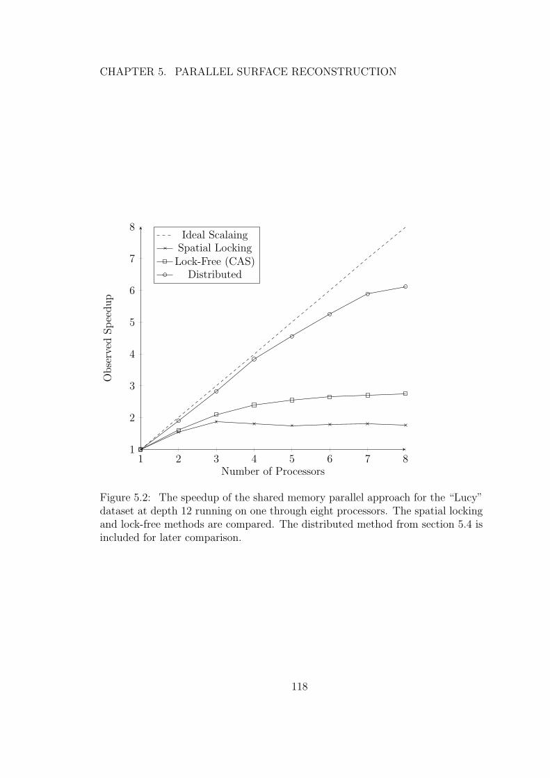
CHAPTER 5. PARALLEL SURFACE RECONSTRUCTION
1 2 3 4 5 6 7 81
2
3
4
5
6
7
8
Number of Processors
Obse
rved
Spee
dup
Ideal ScalaingSpatial LockingLock-Free (CAS)
Distributed
Figure 5.2: The speedup of the shared memory parallel approach for the “Lucy”dataset at depth 12 running on one through eight processors. The spatial lockingand lock-free methods are compared. The distributed method from section 5.4 isincluded for later comparison.
118
CHAPTER 5. PARALLEL SURFACE RECONSTRUCTION
First, for distributive functions, data are shared not only within a level of the
tree, but across all depths of the tree. At the finest levels, the contention for
shared data is very low: since a very small portion of each partition is shared, the
probability of two processors needing concurrent access to a datum are low. At
the coarser levels of the tree, however, the rate of contention becomes very high
and the data associated with the coarsest levels of the tree are updated by each
processor for every computation. Although particularly noticeable when using
a spatial locking scheme, we found that this problem persisted even when we
used an optimistic, lock-free technique that implemented an atomic floating-point
accumulation.
Second, scalability is limited by the large number of global synchronization
barriers that are required to evaluate multiple functions correctly. Each streaming
pass, P , across the octree is a pipeline of functions P = {N1, N2, ..., Nn} that
are executed in sequence. Although the data dependencies are such that the
evaluation of Ni(o) cannot depend on the result of Ni(o′), it is possible that Ni
may depend on Nj if i > j. The implication of this in a parallel setting is
that function Ni cannot be evaluated for a particular slice until Nj has completed
processing in dependent slices on all processors, requiring a global synchronization
barrier to be introduced between each function, for each processing slice. For all
but the very largest reconstructions, the overhead of this is prohibitive. Although
this synchronization frequency can be reduced by processing functions over slabs
119
CHAPTER 5. PARALLEL SURFACE RECONSTRUCTION
of data formed from multiple octree slices, the associated increase in in-core
memory usage results in an undesirable practical limitation on the reconstruction
resolution.
5.4 Distributed Memory
To address the scalability issues that arise from using a shared memory, multi-
threaded, architecture we re-evaluated the initial design and opted instead to
use a distributed memory model. In this approach, each processor shares data
explicitly through message passing, rather than implicitly through shared memory.
The advantages of this model over the shared memory approach are as follows:
• Explicit data sharing: One of the major limitations of the shared memory
approach was that data was frequently, and implicitly shared. In the
distributed approach, each processor maintains a private copy of all data
it needs. Thus, data writes during computation can be performed without
the need for synchronization, and data modified on more than one processor
can be easily and efficiently reconciled at the end of each computation pass.
• Scalable I/O and Memory Bandwidth: Without the need for shared
memory space, the system can be run on computing clusters, offering the
potential for greater scalability, due to the increased memory and I/O
bandwidth, and number of processors.
120
CHAPTER 5. PARALLEL SURFACE RECONSTRUCTION
To implement our distributed model, we revert to the simple streaming
implementation from Section 4.3 in which each function is implemented as a
separate streaming pass through the data. While this increases the amount of I/O
performed, it alleviates the need for global, inter-slice, synchronization barriers
that are required to allow multiple functions to be evaluated correctly.
5.4.1 Data Partitioning
Instead of fine-grained, slice-level parallelism, the distributed system uses a
coarse-grained approach: the reconstruction domain is partitioned into p slabs
(where p is the number of processors) along the x-axis given by the x-coordinates
X = {x0, x1, x2, ..., xp}. The nodes from depth d in the octree are split into
partitions Od = {Od1,Od
2, ...,Odp} where Od
p are all nodes o ∈ O such that xp ≤
o.x < xp+1 and o.d = d.
Since the coarse nodes in the tree are frequently shared across all processors,
we designate the first dfull levels in the tree to be part of its own data partition
Ofull, which is not owned by a particular process, and whose processing is carried
out in duplicate by all processors. Since the total data size of Ofull is small, the
added expense of duplicating this computation is significantly smaller than the
cost of managing consistent replication of the data.
Figure 5.3 summarizes the decomposition of the octree into partitions. A
processor Pi is assigned to own and process the nodes inO∗i in a streaming manner.
121
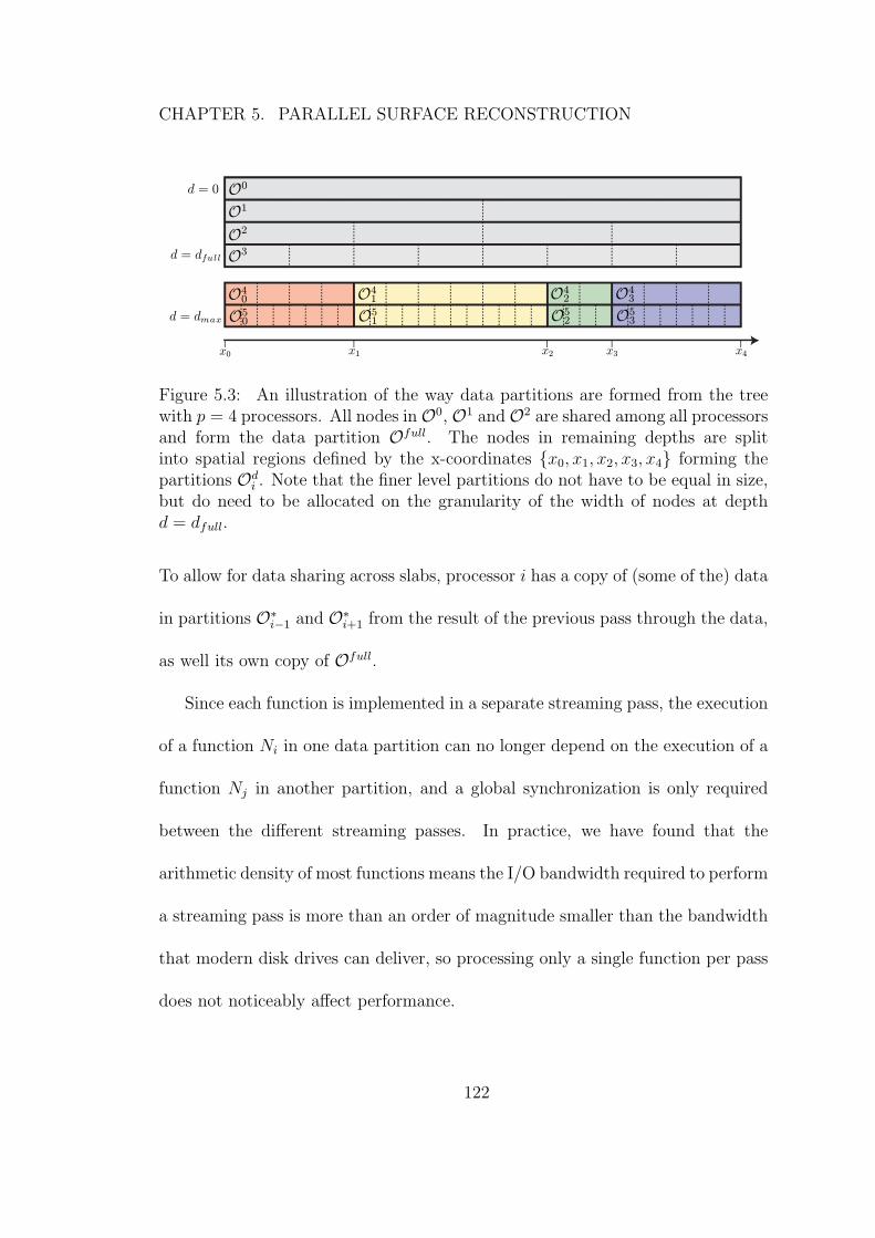
CHAPTER 5. PARALLEL SURFACE RECONSTRUCTION
d = dmax
d = dfull
d = 0
x0 x1 x2 x3 x4
O0
O1
O2
O40 O4
1 O42 O4
3
O3
O50 O5
1 O52 O5
3
Figure 5.3: An illustration of the way data partitions are formed from the treewith p = 4 processors. All nodes inO0, O1 andO2 are shared among all processorsand form the data partition Ofull. The nodes in remaining depths are splitinto spatial regions defined by the x-coordinates {x0, x1, x2, x3, x4} forming thepartitions Od
i . Note that the finer level partitions do not have to be equal in size,but do need to be allocated on the granularity of the width of nodes at depthd = dfull.
To allow for data sharing across slabs, processor i has a copy of (some of the) data
in partitions O∗i−1 and O∗
i+1 from the result of the previous pass through the data,
as well its own copy of Ofull.
Since each function is implemented in a separate streaming pass, the execution
of a function Ni in one data partition can no longer depend on the execution of a
function Nj in another partition, and a global synchronization is only required
between the different streaming passes. In practice, we have found that the
arithmetic density of most functions means the I/O bandwidth required to perform
a streaming pass is more than an order of magnitude smaller than the bandwidth
that modern disk drives can deliver, so processing only a single function per pass
does not noticeably affect performance.
122
CHAPTER 5. PARALLEL SURFACE RECONSTRUCTION
5.4.2 Load Balancing
Because the octree is an adaptive structure, its nodes are non-uniformly
distributed over space. This presents a challenge when choosing the partition
bounds X in order to most optimally allocate work across all processors. To
minimize workload skew, each partition Odi should be approximately the same
size (assuming that the processing time of each node is, on average, constant).
Because we wish to perform the allocation of nodes to partitions before the
tree has been created, we use the input point-set to estimate the the density of
nodes in the tree. Since an octree node may not straddle two data partitions,
the partition bounds X must be chosen such that each xi is a multiple of 2−dfull
(i.e. the width of the coarsest nodes in the high resolution tree). We use a simple
greedy algorithm to allocate X: given an ideal partition size of Nideal = Np, we
grow a partition starting at x = 0 until the partition size would exceed Nideal. We
then over-allocate or under-allocate the partition depending on which minimizes
|Ni −Nideal|. The procedure is continued along the x-axis until all partition sizes
have been determined.
5.4.3 Replication and Merging of Shared Data
Once data have been modified by a processor, the changes need to be reconciled
and replicated between processors. As discussed previously, the majority of the
123
CHAPTER 5. PARALLEL SURFACE RECONSTRUCTION
shared updates performed by the reconstructor are of the form o.v = o.v + v; that
is, accumulating some floating-point scalar or vector quantity into tree nodes. The
merge process for a process Pi is as follows:
1. If Pi has written to Oi−1 and Oi+1, send data to Pi−1 and Pi+1 respectively.
2. If Pi−1 and Pi+1 have modified data in Oi, wait for all data to be received.
3. Merge the received data blocks with the data in Oi (an efficient vector
addition operation).
Once data has been reconciled, the updated data can then be redistributed to
other processes as follows:
1. If Oi has been updated and is needed by Pi−1 or Pi+1 in the next pass, send
Oi to the neighboring processors.
2. If Oi−1 and Oi+1 have modified data needed for the next pass, wait for all
updated data blocks.
In practice, there are a number of optimizations that are made to the merge
process. First, because the streams underlying the data partitions are managed
in memory as blocks for disk streaming purposes, only modified blocks need be
sent between processors, not the entire data partition. In fact, only a very small
portion of data in Oi−1 and Oi+1 are ever read from or written to Pi (only the
data in slices immediately adjacent to Oi), so the neighboring data streams are
124
CHAPTER 5. PARALLEL SURFACE RECONSTRUCTION
sparsely populated during replication. Second, because each processor streams
through the data partitions, changes made to data can be sent asynchronously
to other processing nodes as each block in the stream is finalized, rather than
after the pass is complete, hiding the latency involved in many message passing
operations.
As in the shared-memory model, the tree construction and the solution of the
Laplacian cannot be merged and replicated as efficiently.
5.4.4 Tree Construction
To maximize the parallel processing capability of our system, the construction
of the octree itself is performed in parallel. The input point-set P is partitioned
during pre-processing into segments P = {P1, ...,Pp} where Pi contains all points
xi ≤ p.x < xi+1 (where xi is the partitioning bounds separating the domain of
process Pi−1 from process Pi).
The first challenge presented in the construction of the tree is the different
topological structure created in Ofull by each processor. To facilitate the efficient
merging of data in later steps, it is desirable to have a consistent coarse resolution
tree. Although it is possible to merge each of the coarse resolution trees after the
first pass, we take a simpler approach: because the coarse resolution tree is small,
we pre-construct it as a fully refined octree of depth dfull + 1.
The second challenge is that in the initial phases of the reconstruction, a point
125
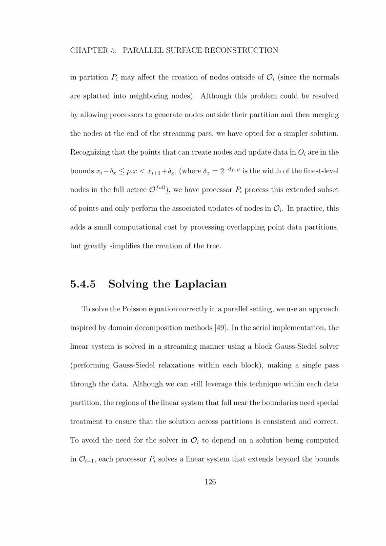
CHAPTER 5. PARALLEL SURFACE RECONSTRUCTION
in partition Pi may affect the creation of nodes outside of Oi (since the normals
are splatted into neighboring nodes). Although this problem could be resolved
by allowing processors to generate nodes outside their partition and then merging
the nodes at the end of the streaming pass, we have opted for a simpler solution.
Recognizing that the points that can create nodes and update data in Oi are in the
bounds xi−δx ≤ p.x < xi+1+δx, (where δx = 2−dfull is the width of the finest-level
nodes in the full octree Ofull), we have processor Pi process this extended subset
of points and only perform the associated updates of nodes in Oi. In practice, this
adds a small computational cost by processing overlapping point data partitions,
but greatly simplifies the creation of the tree.
5.4.5 Solving the Laplacian
To solve the Poisson equation correctly in a parallel setting, we use an approach
inspired by domain decomposition methods [49]. In the serial implementation, the
linear system is solved in a streaming manner using a block Gauss-Siedel solver
(performing Gauss-Siedel relaxations within each block), making a single pass
through the data. Although we can still leverage this technique within each data
partition, the regions of the linear system that fall near the boundaries need special
treatment to ensure that the solution across partitions is consistent and correct.
To avoid the need for the solver in Oi to depend on a solution being computed
in Oi−1, each processor Pi solves a linear system that extends beyond the bounds
126
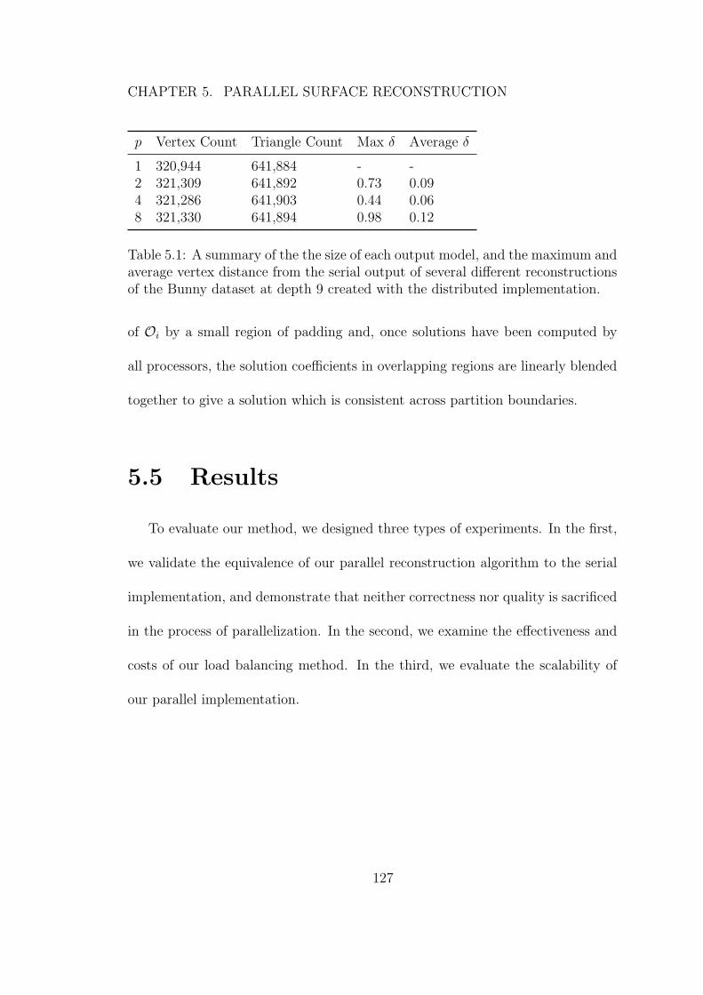
CHAPTER 5. PARALLEL SURFACE RECONSTRUCTION
p Vertex Count Triangle Count Max δ Average δ
1 320,944 641,884 - -2 321,309 641,892 0.73 0.094 321,286 641,903 0.44 0.068 321,330 641,894 0.98 0.12
Table 5.1: A summary of the the size of each output model, and the maximum andaverage vertex distance from the serial output of several different reconstructionsof the Bunny dataset at depth 9 created with the distributed implementation.
of Oi by a small region of padding and, once solutions have been computed by
all processors, the solution coefficients in overlapping regions are linearly blended
together to give a solution which is consistent across partition boundaries.
5.5 Results
To evaluate our method, we designed three types of experiments. In the first,
we validate the equivalence of our parallel reconstruction algorithm to the serial
implementation, and demonstrate that neither correctness nor quality is sacrificed
in the process of parallelization. In the second, we examine the effectiveness and
costs of our load balancing method. In the third, we evaluate the scalability of
our parallel implementation.
127
CHAPTER 5. PARALLEL SURFACE RECONSTRUCTION
± = 0.0
± = 0.25
± = 1.0
± = 0.5
± = 0.0625
Figure 5.4: The distribution of error across the p = 8 model, when compared tothe serial model. The color is used to show δ values over the surface with δ = 0.0colored blue and δ = 1.0 colored red. The scale is non-linear to highlight smallvalues of δ.
5.5.1 Correctness
We wish to ensure that the surface generated by the parallel implementation
is equivalent in quality to the serial implementation. In particular, we want to
ensure that the model does not significantly change as the number of processors
increases, and that any differences that do exist do not accumulate near partition
boundaries.
To test this, we ran an experiment using the distributed implementation,
reconstructing the Stanford Bunny model at depth 9 using 1, 2, 4, and 8
processors. We then compared the model generated with only one processor
Mserial, to the models generated with multiple processors Mi by computing an
error value δ at each vertex of Mi measured as the Euclidean distance to the
nearest point on the triangle mesh of Mserial. The units of δ are scaled to represent
the resolution of the reconstruction so that 1.0δ = 2−d (the width of the finest
128
CHAPTER 5. PARALLEL SURFACE RECONSTRUCTION
nodes in the tree).
Table 5.1 presents the results of this experiment. Some differences in the
output are expected between different numbers of processors because of the lack
of commutativity of floating-point arithmetic. The results show that, in all cases,
the average error is low and the maximum error is bounded within the size of the
finest tree nodes. They also show that error does not significantly change as the
number of processors increases. The image in Figure 5.4 shows the distribution
of error across the mesh for p = 8, and is typical of our multiple processor results.
The image highlights that error is evenly distributed across the mesh, and that
the only significant error occurs along the shape crease along the bottom of the
bunny’s back leg. These errors are the result of a different choice in triangulation
along the sharper edges of the model (e.g. around the bottom of the Bunny).
5.5.2 Skew
To evaluate the efficiency and cost of our load balancing method we ran the
algorithm on the head of the David for a range of different values for dfull, and
different numbers of processors. The results are presented in Figure 5.5, which
plots |max pi−P
pi
p| for 2, 4, 8 and 16 processors, where pi represents the amount
of work allocated to processor i. From these results, we can make a number of
observations.
For this particular dataset, when dfull ≥ 7, the workload is very well balanced,
129
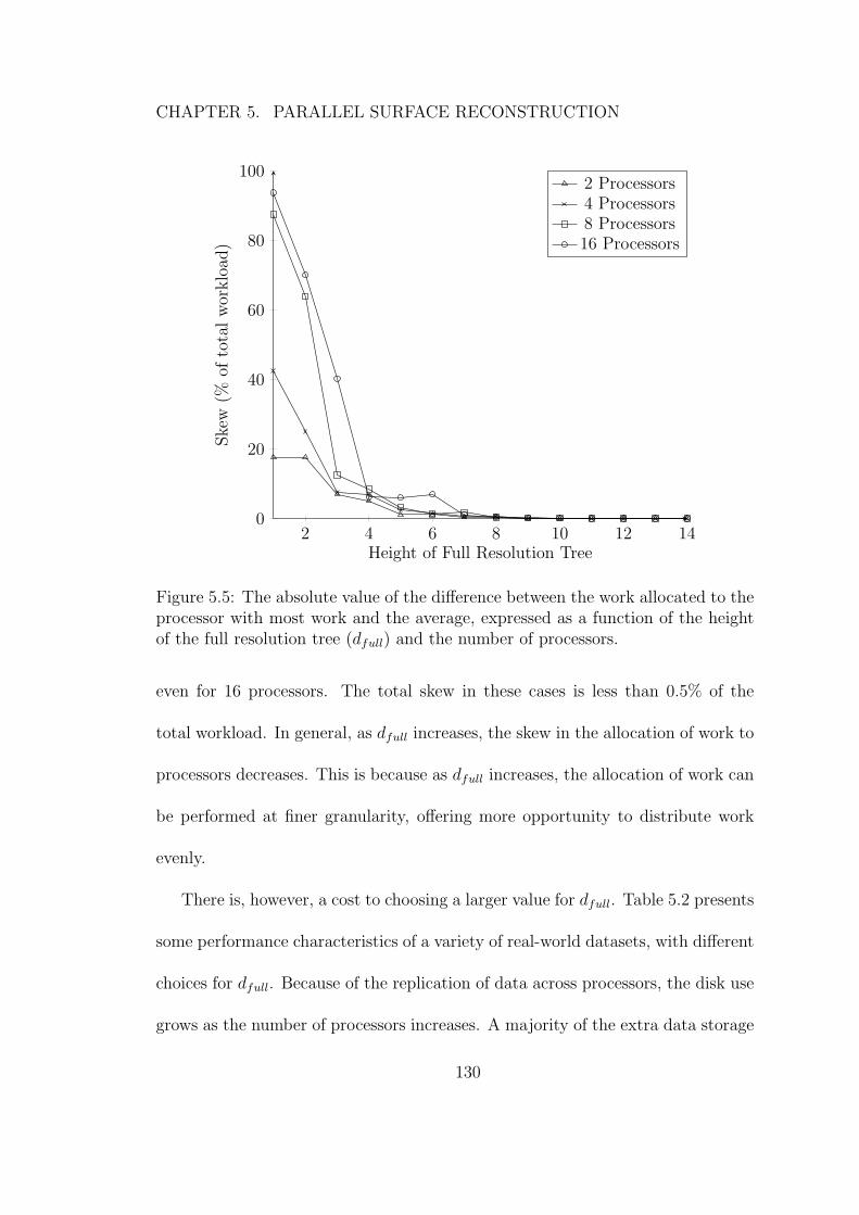
CHAPTER 5. PARALLEL SURFACE RECONSTRUCTION
2 4 6 8 10 12 140
20
40
60
80
100
Height of Full Resolution Tree
Ske
w(%
ofto
talw
orklo
ad)
2 Processors4 Processors8 Processors16 Processors
Figure 5.5: The absolute value of the difference between the work allocated to theprocessor with most work and the average, expressed as a function of the heightof the full resolution tree (dfull) and the number of processors.
even for 16 processors. The total skew in these cases is less than 0.5% of the
total workload. In general, as dfull increases, the skew in the allocation of work to
processors decreases. This is because as dfull increases, the allocation of work can
be performed at finer granularity, offering more opportunity to distribute work
evenly.
There is, however, a cost to choosing a larger value for dfull. Table 5.2 presents
some performance characteristics of a variety of real-world datasets, with different
choices for dfull. Because of the replication of data across processors, the disk use
grows as the number of processors increases. A majority of the extra data storage
130
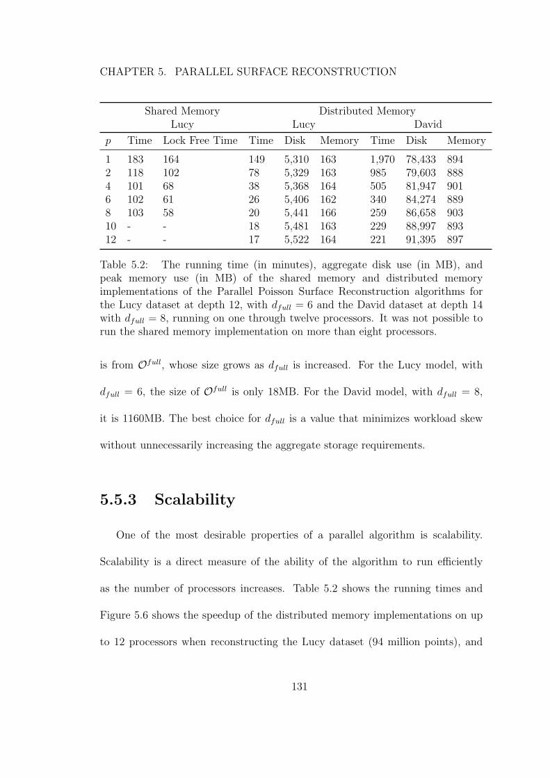
CHAPTER 5. PARALLEL SURFACE RECONSTRUCTION
Shared Memory Distributed MemoryLucy Lucy David
p Time Lock Free Time Time Disk Memory Time Disk Memory
1 183 164 149 5,310 163 1,970 78,433 8942 118 102 78 5,329 163 985 79,603 8884 101 68 38 5,368 164 505 81,947 9016 102 61 26 5,406 162 340 84,274 8898 103 58 20 5,441 166 259 86,658 90310 - - 18 5,481 163 229 88,997 89312 - - 17 5,522 164 221 91,395 897
Table 5.2: The running time (in minutes), aggregate disk use (in MB), andpeak memory use (in MB) of the shared memory and distributed memoryimplementations of the Parallel Poisson Surface Reconstruction algorithms forthe Lucy dataset at depth 12, with dfull = 6 and the David dataset at depth 14with dfull = 8, running on one through twelve processors. It was not possible torun the shared memory implementation on more than eight processors.
is from Ofull, whose size grows as dfull is increased. For the Lucy model, with
dfull = 6, the size of Ofull is only 18MB. For the David model, with dfull = 8,
it is 1160MB. The best choice for dfull is a value that minimizes workload skew
without unnecessarily increasing the aggregate storage requirements.
5.5.3 Scalability
One of the most desirable properties of a parallel algorithm is scalability.
Scalability is a direct measure of the ability of the algorithm to run efficiently
as the number of processors increases. Table 5.2 shows the running times and
Figure 5.6 shows the speedup of the distributed memory implementations on up
to 12 processors when reconstructing the Lucy dataset (94 million points), and
131
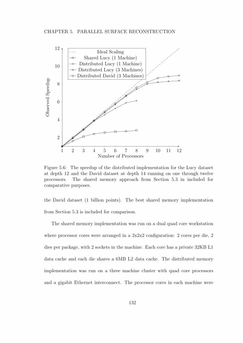
CHAPTER 5. PARALLEL SURFACE RECONSTRUCTION
1 2 3 4 5 6 7 8 9 10 11 12
2
4
6
8
10
12
Number of Processors
Obse
rved
Spee
dup
Ideal ScalingShared Lucy (1 Machine)
Distributed Lucy (1 Machine)Distributed Lucy (3 Machines)Distributed David (3 Machines)
Figure 5.6: The speedup of the distributed implementation for the Lucy datasetat depth 12 and the David dataset at depth 14 running on one through twelveprocessors. The shared memory approach from Section 5.3 in included forcomparative purposes.
the David dataset (1 billion points). The best shared memory implementation
from Section 5.3 is included for comparison.
The shared memory implementation was run on a dual quad core workstation
where processor cores were arranged in a 2x2x2 configuration: 2 cores per die, 2
dies per package, with 2 sockets in the machine. Each core has a private 32KB L1
data cache and each die shares a 6MB L2 data cache. The distributed memory
implementation was run on a three machine cluster with quad core processors
and a gigabit Ethernet interconnect. The processor cores in each machine were
132
CHAPTER 5. PARALLEL SURFACE RECONSTRUCTION
arranged in a 1x2x2 configuration: 2 cores per die, 2 dies per package, with 1
socket per machine. The cache layout is the same as the shared memory machine.
When we examine the scalability of the shared memory implementation, which
uses atomic instructions to manage concurrent updates, we see that the scalability
is severely limited compared to the distributed implementation. One significant
factor affecting the performance is the way in which shared memory data updates
interact with architectural elements of the underlying hardware. When locking
shared data between processors, data that were kept primarily in fast on-chip
memory caches have to be flushed and shared through main memory each time it
is modified to keep separate caches coherent. This forces frequently shared data
to be extremely inefficient to access, with no cache to hide high latency memory
access. Because the distributed implementation does not need to coordinate
writes to the same data, the computation is far more efficient, and cleanly scales
with increasing numbers of processors. The reduced scalability as the number of
processors increases is due to the complete occupancy of all processors on each
machine, causing the algorithm to become memory bandwidth bound.
To highlight the advantages of using multiple machines to run the distributed
implementation, we also ran the distributed implementation on the shared
memory machine. The results of this experiment are shown in Figure 5.6
on the data series labelled “Distributed Lucy (1 machine)”. Although the
distributed implementation performs significantly better than the shared memory
133
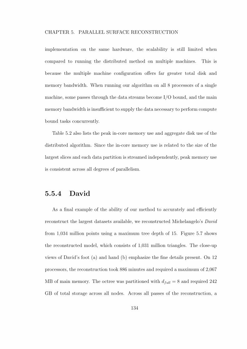
CHAPTER 5. PARALLEL SURFACE RECONSTRUCTION
implementation on the same hardware, the scalability is still limited when
compared to running the distributed method on multiple machines. This is
because the multiple machine configuration offers far greater total disk and
memory bandwidth. When running our algorithm on all 8 processors of a single
machine, some passes through the data streams become I/O bound, and the main
memory bandwidth is insufficient to supply the data necessary to perform compute
bound tasks concurrently.
Table 5.2 also lists the peak in-core memory use and aggregate disk use of the
distributed algorithm. Since the in-core memory use is related to the size of the
largest slices and each data partition is streamed independently, peak memory use
is consistent across all degrees of parallelism.
5.5.4 David
As a final example of the ability of our method to accurately and efficiently
reconstruct the largest datasets available, we reconstructed Michelangelo’s David
from 1,034 million points using a maximum tree depth of 15. Figure 5.7 shows
the reconstructed model, which consists of 1,031 million triangles. The close-up
views of David’s foot (a) and hand (b) emphasize the fine details present. On 12
processors, the reconstruction took 886 minutes and required a maximum of 2,067
MB of main memory. The octree was partitioned with dfull = 8 and required 242
GB of total storage across all nodes. Across all passes of the reconstruction, a
134
CHAPTER 5. PARALLEL SURFACE RECONSTRUCTION
Figure 5.7: A reconstruction of the David model at depth 15.
135
CHAPTER 5. PARALLEL SURFACE RECONSTRUCTION
total of 2,178 GB of disk I/O was performed. Of the 28 GB of total network I/O,
51 MB was performed synchronously at the end of the data passes.
136
Chapter 6
Conclusion
In this dissertation we have described a new technique for surface
reconstruction that is designed to meet the demands of modern reconstruction
datasets.
In Chapter 3, we described the Poisson Surface Reconstruction technique
which takes a global implicit function fitting approach to solving the surface
reconstruction problem by contructing an approximation to the indicator function
(χ) of the unknown surface. Using an oriented pointset, we construct an
approximation to the gradient of the indicator function (~V ≈ ∇χ), compute the
divergence (∇ ·∇χ) and solve the Poisson problem ∇2χ = ∇ · ~V for the unknown
χ. The reconstructed surface is then extracted as a level-set of χ.
We exploit the fact that the indicator function is constant almost everywhere
(and thus, the gradient is zero almost everywhere), and represent both the
137
CHAPTER 6. CONCLUSION
indicator function and its gradient within an adaptive, hierarchical function space
defined over an octree. This adaptive representation makes the algorithm output-
sensitive and have a spatial complexity of O(n2) and temporal complexity of
O(n2 log n).
Because we use a global approach to the problem, our method is highly robust
to noise and other anomalies found in real-world scan data. Through experiments,
we have shown this method to be competitive in terms of running time and often
superior in quality to a wide range of existing methods. One of the practical
limitations of our method is that the octree-based representation of the indicator
function was required to be in main memory at all times. This limited the
maximum size of reconstructions we could perform.
In Chapter 4, we addressed the challenge of reconstructing extremely large
datasets by introducing a streaming framework to the problem. Using the
knowledge that each computation involved in the Poisson reconstruction method
only requires a small portion of the octree data at any one time, the octree can
be stored on disk and data can be loaded into main memory only when required.
To make the transfer of data to and from disk as efficient as possible, we use a
streaming approach: a given piece of data is read from disk into memory once
when it is first needed for a computation and is written back to disk (thus freeing
memory) after it is no longer needed for further computation. Because data at
different depths of the octree have significantly varying lifetimes, we use a multi-
138
CHAPTER 6. CONCLUSION
level approach to streaming: each level of the tree is managed and streamed
independently. This allows the portion of the octree data in memory at any one
time to be as small as possible. Through pipelining and the use of a cascadic
multigrid solver, the entire reconstruction process is implemented in just three
passes across the octree data.
We demonstrated that our streaming approach removes the limitations on
memory size by reconstructing several large models including Michelangelo’s
Awakening from 431 million data points. For this model, the reconstruction
created an octree containing 106GB of data, while using only 2.1GB of main
memory. Despite needing to stream large amounts of data to and from disk,
the running time was only approximately 20 percent slower than the in-core
implementation.
Finally, in Chapter 5, we extended the streaming technique to run in parallel on
multi-core CPUs and CPU-based computing clusters. We used the knowledge of
data dependencies gained from the streaming work to partition the ocree data and
evaluate a given computation across all nodes in a partition in parallel. Using a
distributed memory model, we resolved the need for frequent data synchronization
by replicating commonly updated data across all processors and merging results
together at the end of a computation pass. We have shown that our distributed
implementation is effective when running on a single computer with multi-core
CPUs or on a computing cluster. On a multi-core, multi-processor workstation
139
CHAPTER 6. CONCLUSION
with 8 cores, we can reconstruct surfaces 6 times faster than the non-parallel
approach, and on a 12 processor cluster, we can reconstruct surfaces 9.3 times
faster.
6.1 Future Work
There are a number of avenues for future work, including extending our parallel
method to run on graphics processing units (GPUs) and developing a rigourous
way for evaluating and comparing surface reconstruction techniques. We now
discuss these ideas in more detail.
6.1.1 A GPU Implementation
Modern graphics processing units (GPUs) are among the most powerful
processing chips that exist today. State of the art GPUs are capable of over
2.5 teraflops of single precision floating-point arithmetic and have in excess of 250
GB/s of memory bandwidth – orders of magnitude more than current multi-core
CPUs. The hardware-based scheduler in a GPU is capable of scheduling tens of
thousands of active, lightweight, hardware threads onto hundreds of processing
cores. Although originally designed and used specifically as specialized hardware
to accelerate the rendering of complex 3D scenes, the GPU has been repositioned
as a high performance general purpose co-processor.
140
CHAPTER 6. CONCLUSION
The work of Zhou et. al. [59] implemented the in-core algorithm that we
presented in Chapter 3 on the GPU. This implementation has shown that the
Poisson Surface Reconstruction method has sufficient inherent data parallelism to
perform well on the GPU, with performance speed-ups sufficient to reconstruct
small models in real-time. A significant limitation of their approach, however,
is that it relies on the entire dataset and octree residing entirely within GPU
memory.
In the future, we would like to explore a GPU implementation that is a hybrid
of the shared-memory and distributed memory approaches from Chapter 5. A
distributed system is required to run a computation across multiple GPUs (even
when they are in the same host) because GPU memory space is private and is
not shared with other GPUs or the host systems. For the computations within a
single GPU a shared memory approach is more appropriate.
6.1.2 A Surface Reconstruction Benchmark
Standardized benchmarks have been used in a variety of disciplines to measure
the relative performance and correctness of algorithms, ranging from measuring
the performance of numerical algorithms as in the LINPACK linear algebra
benchmark [19], to comparing shape-matching [48] and segmentation [14] methods
in computer graphics.
Unfortunately, there has been no standard benchmark established for
141
CHAPTER 6. CONCLUSION
evaluating reconstruction algorithms. The lack of consistency in testing
methodology makes it difficult to make direct comparisons between methods, and
synthetic data experiments often fail to capture the subtle characteristics of real
scanned data, making the test ineffective in measuring real-world reconstruction
ability. Experiments run with real-world data do present a more realistic view,
but error is often hard to measure and quantify, since no ground truth surface is
available, making direct, objective, comparisons between methods difficult. Part
of the challenge is that surface reconstruction is used in numerous applications,
each of which have their own unique requirements.
In the future, we would like to develop a benchmark that would consist of a
battery of carefully designed experiments that, though synthetically generated,
would accurately model individual sources of error found in real-world data. For
example, one test could model non-uniform data by overlaying a set of artificially
generated scans of an object. Because these scans are artificially generated (e.g.
via ray tracing), the influence of other aspects of real data, such as noise and
misalignment can be excluded. The results of each of these experiments would be
measured by a collection of error metrics which would include geometry based
methods that measure the distance between surfaces, as well as image based
methods which could capture preceptual error by comparing renderings of a
ground truth and reconstructed model from different viewpoints under a variety
of lighting conditions.
142

CHAPTER 6. CONCLUSION
We expect such a benchmark to have two main practical uses: First, it
would allow different reconstruction methods to be compared in an objective
way while capturing key aspects of what makes surface reconstruction from real
data a difficult problem. Second, such a benchmark can be used to drive future
development of better surface reconstruction methods by helping identify the
limitations of existing techniques.
143
Bibliography
[1] Agarwal, R. C., Gustavson, F. G., and Zubair, M. A high
performance parallel algorithm for 1-d FFT. In Proceedings of the 1994
Conference on Supercomputing (1994), pp. 34–40.
[2] Ahn, M., Guskov, I., and Lee, S. Out-of-core remeshing of large
polygonal meshes. In Proceedings on the Conference on Visualization (2006),
vol. 12, pp. 1221–1228.
[3] Alexa, M., Behr, J., Cohen-Or, D., Fleishman, S., Levin, D., and
Silva, C. T. Point set surfaces. In IEEE VIS (2001), pp. 21–28.
[4] Amenta, N., Choi, S., and Kolluri, R. Power crust. Sixth ACM
Symposium on Solid Modeling and Applications (2001), 249–260.
[5] Amenta, N., Choi, S., and Kolluri, R. K. The power crust, unions of
balls, and the medial axis transform. Computational Geometry: Theory and
Applications 19 (2000), 127–153.
144
BIBLIOGRAPHY
[6] Attali, D., Cohen-Steiner, D., and Edelsbrunner, H. Extraction
and simplification of iso-surfaces in tandem. In Symposium on Geometry
Processing (2005).
[7] Barnard, S. T., and Fischler, M. A. Computational stereo. ACM
Compututing Surveys 14, 4 (1982), 553–572.
[8] Bernardini, F., Mittleman, J., Rushmeier, H., Silva, C., and
Taubin, G. The ball-pivoting algorithm for surface reconstruction. IEEE
Transactions on Visualization and Computer Graphics 5, 4 (1999), 349–359.
[9] Bernardini, F., Rushmeier, H., Martin, I. M., Mittleman, J., and
Taubin, G. Building a digital model of Michelangelo’s Florentine Pieta.
IEEE Computer Graphics and Applications 22 (2002), 59–67.
[10] Blinn, J. F. A generalization of algebraic surface drawing. ACM
Transactions on Graphics 1, 3 (1982), 235–256.
[11] Bornemann, F., and Krause, R. Classical and cascadic multigrid
– a methodological comparison. In Proceedings of the 9th International
Conference on Domain Decomposition Methods (1996), pp. 64–71.
[12] Brown, B. J., and Rusinkiewicz, S. Global non-rigid alignment of 3D
scans. ACM Transactions on Graphics 26, 3 (July 2007), 21.
145
BIBLIOGRAPHY
[13] Carr, J. C., Beatson, R. K., Cherrie, J. B., Mitchell, T. J.,
Fright, W. R., McCallum, B. C., and Evans, T. R. Reconstruction
and representation of 3d objects with radial basis functions. In ACM
Transactions on Graphics, Proceedings of ACM SIGGRAPH (2001), pp. 67–
76.
[14] Chen, X., Golovinskiy, A., and Funkhouser, T. A Benchmark for 3D
Mesh Segmentation. ACM Transactions on Graphics, Proceedings of ACM
SIGGRAPH 28, 3 (8 2009).
[15] Chen, Y., and Medioni, G. Description of complex objects from multiple
range images using an inflating balloon model. Computer Vision Image
Understanding 61, 3 (1995), 325–334.
[16] Cignoni, P., Montani, C., Rocchini, C., and Scopigno, R. External
memory management and simplification of huge meshes. IEEE Transactions
on Visualization and Computer Graphics 9 (2003).
[17] Curless, B., and Levoy, M. A volumetric method for building complex
models from range images. In ACM Transactions on Graphics, Proceedings
of ACM SIGGRAPH (1996), pp. 303–312.
[18] Dey, T., and Goswami, S. Provable surface reconstruction from noisy
samples. In Annual Symposium on Computational Geometry (2004), pp. 330–
339.
146
BIBLIOGRAPHY
[19] Dongarra, J. The LINPACK Benchmark: An explanation. Proceedings of
the 1st International Conference on Supercomputing (1988), 456–474.
[20] Edelsbrunner, H., and Mucke, E. P. Three-dimensional alpha shapes.
ACM Transactions on Graphics 13, 1 (1994), 43–72.
[21] Franke, R. Scattered data interpolation: Tests of some methods.
Mathematics of Computation 38, 157 (1982), 181–200.
[22] George, A., and Rashwan, H. Auxiliary storage methods for solving
finite element systems. SIAM Journal on Scientific and Statistical Computing
6 (1985).
[23] Grinspun, E., Krysl, P., and Schroder, P. CHARMS: a simple
framework for adaptive simulation. In ACM Transactions on Graphics,
Proceedings of ACM SIGGRAPH (2002), pp. 281–290.
[24] Hardwick, J. C. Implementation and evaluation of an efficient parallel
Delaunay triangulation algorithm. In Proceedings of the 9th Annual ACM
Symposium on Parallel Algorithms and Architectures (1997), pp. 23–25.
[25] Hoppe, H., DeRose, T., Duchamp, T., McDonald, J., and
Stuetzle, W. Surface reconstruction from unorganized points. Computer
Graphics 26 (1992), 71–78.
147
BIBLIOGRAPHY
[26] Horn, B. K. P. Shape from shading: A method for obtaining the shape of
a smooth opaque object from one view. PhD thesis, Department of Electrical
Engineering, Massachusetts Institute of Technology, 1970.
[27] Isenburg, M., and Lindstrom, P. Streaming meshes. In Proceedings of
the Conference on Visualization (2005).
[28] Isenburg, M., Lindstrom, P., Gumhold, S., and Shewchuk, J.
Streaming compression of tetrahedral volume meshes. In Proceedings of
Graphics Interface 2006 (2006).
[29] Isenburg, M., Lindstrom, P., Gumhold, S., and Snoeyink, J.
Large mesh simplification using processing sequences. In Proceedings of the
Conference on Visualization (2003).
[30] Isenburg, M., Liu, Y., Shewchuk, J., and Snoeyink, J. Streaming
computation of Delaunay triangulations. ACM Transactions on Graphics 25
(2006).
[31] Kazhdan, M. Reconstruction of solid models from oriented point sets. In
Eurographics Symposium on Geometry Processing (2005), p. 73.
[32] Kazhdan, M., Klein, A., Dalal, K., and Hoppe, H. Unconstrained
isosurface extraction on arbitrary octrees. In Eurographics Symposium on
Geometry Processing 2007 (2007), pp. 125–133.
148
BIBLIOGRAPHY
[33] Levin, D. The approximation power of moving least-squares. Mathematics
of Computation 67 (1998), 1517–1531.
[34] Levoy, M., Pulli, K., Curless, B., Rusinkiewicz, S., Koller, D.,
Pereira, L., Ginzton, M., Anderson, S., Davis, J., Ginsberg, J.,
Shade, J., and Fulk, D. The digital Michelangelo project: 3D scanning
of large statues. In ACM Transactions on Graphics, Proceedings of ACM
SIGGRAPH (July 2000).
[35] Levoy, M., and Whitted, T. The use of points as a display primitive.
Tech. Rep. 22, The University of North Carolina at Chapel Hill, 1985.
[36] Lindstrom, P., and Silva, C. A memory insensitive technique for large
model simplification. In Proceedings of the Conference on Visualization
(2001).
[37] Lorensen, W., and Cline, H. Marching cubes: A high resolution
3D surface reconstruction algorithm. ACM Transactions on Graphics,
Proceedings of ACM SIGGRAPH (1987), 163–169.
[38] Losasso, F., Gibou, F., and Fedkiw, R. Simulating water and smoke
with an octree data structure. ACM Transactions on Graphics, Proceedings
of ACM SIGGRAPH 23 (2004), 457–462.
149
BIBLIOGRAPHY
[39] Manson, J., Petrova, G., and Schaefer, S. Streaming surface
reconstruction using wavelets. Computer Graphics Forum 27, 5 (2008), 1411–
1420.
[40] Moreland, K., and Angel, E. The FFT on a GPU. In HWWS
’03: Proceedings of the ACM SIGGRAPH/EUROGRAPHICS conference on
Graphics Hardware (2003), pp. 112–119.
[41] Morton, G. A computer oriented geodetic data base; and a new technique
in file sequencing. Tech. rep., IBM, 1966.
[42] Muraki, S. Volumetric shape description of range data using “blobby
model”. In ACM Transactions on Graphics, Proceedings of ACM SIGGRAPH
(1991), pp. 227–235.
[43] Ohtake, Y., Belyaev, A., Alexa, M., Turk, G., and Seidel, H.-P.
Multi-level partition of unity implicits. ACM Transactions on Graphics 22,
3 (2003), 463–470.
[44] Pajarola, R. Stream-processing points. In Proceedings of the Conference
on Visualization (2005).
[45] Parzen, E. On estimation of a probability density function and mode. The
Annals of Mathematical Statistics 33 (1962), 1065–1076.
150
BIBLIOGRAPHY
[46] Schall, O., Belyaev, A., and Seidel, H.-P. Error-guided adaptive
Fourier-based surface reconstruction. Computer Aided Design 39, 5 (2007),
421–426.
[47] Shekhar, R., Fayyad, E., Yagel, R., and Cornhill, J. Octree-
based decimation of marching cubes surfaces. In IEEE Visualization (1996),
pp. 335–342.
[48] Shilane, P., Min, P., Kazhdan, M., and Funkhouser, T. The
Princeton Shape Benchmark. In SMI04: Proceedings of the Shape Modeling
International 2004 (2004), pp. 167–178.
[49] Smith, B., Bjorstad, P., and Gropp, W. Domain Decomposition:
Parallel Multilevel Methods for Elliptic Partial Differential Equations.
Cambridge University Press, 2004.
[50] Snavely, N., Seitz, S. M., and Szeliski, R. Modeling the world from
internet photo collections. International Journal of Computer Vision 80, 2
(2008), 189–210.
[51] Taubin, G. Estimation of planar curves, surfaces, and nonplanar space
curves defined by implicit equations with applications to edge and range
image segmentation. IEEE Transactions Pattern Analysis and Machine
Intelligence 13, 11 (1991), 1115–1138.
151
BIBLIOGRAPHY
[52] Toledo, S. A survey of out-of-core algorithms in numerical linear algebra.
In External Memory Algorithms and Visualization, J. Abello and J. Vitter,
Eds. American Mathematical Society Press, 1999.
[53] Vo, H., Callahan, S., Lindstrom, P., Pascucci, V., and Silva,
C. Streaming simplification of tetrahedral meshes. IEEE Transactions on
Visualization and Computer Graphics 13 (2007).
[54] Westermann, R., Kobbelt, L., and Ertl, T. Real-time exploration of
regular volume data by adaptive reconstruction of iso-surfaces. The Visual
Computer 15 (1999), 100–111.
[55] Wilhelms, J., and Gelder, A. V. Octrees for faster isosurface generation.
ACM Transactions on Graphics 11 (1992), 201–227.
[56] Wu, J., and Kobbelt, L. A stream algorithm for the decimation of massive
meshes. In Proceedings of the Conference on Graphics Interface (2003).
[57] Zhang, Z. Iterative point matching for registration of free-form curves and
surfaces. International Journal of Computer Vision 13, 2 (1994), 119–152.
[58] Zhao, H.-K., Osher, S., and Fedkiw, R. Fast surface reconstruction
using the level set method. In VLSM ’01: Proceedings of the IEEE Workshop
on Variational and Level Set Methods (VLSM’01) (Washington, DC, USA,
2001), IEEE Computer Society, p. 194.
152

BIBLIOGRAPHY
[59] Zhou, K., Gong, M., Huang, X., and Guo, B. Highly parallel surface
reconstruction. Tech. Rep. 53, Microsoft Research, 2008.
153
Vita
Matthew Grant Bolitho was born on July 11, 1982 in Nelson, New Zealand.
He earned a Bachelor of Science (B.Sc.) degree from the University of Auckland
(Auckland, New Zealand) in 2003 and a Bachelor of Science, Honours degree
(B.Sc., Hons) with First-Class Honours in Computer Science from the University
of Auckland in 2004. Matthew then earned his Masters of Science in Engineering
(M.S.E.) from the Johns Hopkins University (Baltimore, Maryland) in 2007 before
entering Ph.D. candidacy. His research interests include parallel computing and
the construction, processing, and visualization of large geometric datasets.
154