The Rebound Effect for Automobile Travel: Asymmetric Response to Price Changes and Novel Features of the 2000s

Kent M. Hymel

Kenneth A. Small

August 14, 2014

Hymel: Dept. of Economics, California State University at Northridge; kent.hymel@csun.edu Small: Dept. of Economics, University of California at Irvine; ksmall@uci.edu

JEL Codes: Q41, R41, L91 Keywords: Rebound effect, VMT elasticity, Gasoline demand, Asymmetric response

Abstract

Previous research suggests that the elasticity of light-duty motor vehicle travel with respect to fuel cost, known as the “rebound effect,” is modest in size and probably declined in magnitude between the 1960s and the late 1990s. However, turmoil in energy markets during the early 2000s has raised new questions about the stability of this elasticity. Using panel data on U.S. states, we revisit the simultaneous-equations methodology of Small and Van Dender (2007) and Hymel et al. (2010) to see whether structural parameters have changed. Using data through 2009, we confirm the earlier finding of a rebound effect that declines in magnitude with income, but we also find an upward shift in its magnitude of about 0.025 during the years 2003-2009. In addition, we find that the rebound effect is much greater in magnitude in years when gasoline prices are rising than when they are falling. It is also greater during times of media attention and price volatility, which explains about half the upward shift just mentioned.

Acknowledgement

We are grateful to the University of California Center for Energy and Environmental Economics and the Environmental Protection Agency for financial support. We thank Kevin Bolon, Jefferson Cole, Sarah Froman, Kenneth Gillingham, David Greene, Gloria Helfand, Sharyn Lie, James Sallee, Michael Shelby, and seminar participants at Cornell, Yale, CSU Long Beach, and the International Transportation Economics Association for valuable comments at various stages of the work described here.

The Rebound Effect for Automobile Travel: Asymmetric Response to Price Changes and Other Quirks of the 2000s

1. Introduction

Many empirical quantities determine the effectiveness of energy policies toward light-

duty motor vehicles. Analysts have come increasingly to appreciate the importance of one: the

elasticity of vehicle travel with respect to fuel cost, the latter defined as the ratio of fuel price to

fuel efficiency. If it is large, this elasticity policy evaluation in two notable ways. First, it tends to

undermine the effectiveness of direct controls such as the Corporate Average Fuel Efficiency

(CAFE) regulations in the United States. This is because the induced travel offsets some of the

energy savings that would otherwise occur—the origin of the name “rebound effect.” Second,

external costs of motor vehicle travel that are not directly related to energy use—mainly

congestion, accidents, and local air pollution—can loom large in a cost-benefit analysis of

efficiency regulations; they therefore magnify the differences in cost-effectiveness between

policy measures that discourage driving versus those that encourage driving.

The rebound effect is often measured as the negative of the elasticity of driving with

respect to fuel cost per unit distance—also known as the price-elasticity of vehicle miles of travel

(VMT), or simply the “VMT elasticity.” This “direct” rebound effect is typically expressed as a

percentage: for example, a VMT elasticity of -0.20 corresponds to a rebound effect of 20%. Most

demand models assume that fuel efficiency enters the VMT decision only via its role in

determining the per-mile price of driving, so that the elasticities of VMT with respect to fuel

price and fuel intensity (the reciprocal of fuel efficiency) are identical. We follow this practice,

except where we report testing whether VMT indeed responds the same way to fuel price and to

fuel intensity.

A substantial body of earlier empirical evidence mostly supported a long-run rebound

effect of 15% to 30% over the last few decades of the twentieth century.1 Differences among the

studies demonstrate the importance of model specification: for example, the way dynamics are

dealt with, e.g. by whether or not lagged effects and autoregressive errors are accounted for.

1 For literature reviews, see Greening et al. (2000), Small and Van Dender (2007), and Hymel et al. (2010). For meta-analyses of results from these mostly pre-2000 studies, see Goodwin et al. (2004), Graham and Glaister (2004), and Brons et al. (2008).

1

Small and Van Dender (2007) conclude that omitting dynamics is likely to cause the short-run

rebound effect to be overestimated, and to obscure the relationship between short and long run.2

In addition, results of US studies are sensitive to how they account for the influence of the US

Corporate Average Fuel Efficiency (CAFE) standards, which went into effect in 1978.

More recent literature has extended the earlier literature in several directions. Two

directions of special interest are how the rebound effect may change over time, and whether its

measurement is sensitive to bias due to omitted variables. We begin with our own previous work,

on which the current paper builds.

Small and Van Dender (2007), using data on individual states in the US for years 1966-

2001, estimate a three-equation model system in which VMT, vehicle ownership, and fuel

efficiency are simultaneously determined. They find that ignoring this endogeneity of fuel

efficiency (in particular, that the fuel efficiency chosen jointly by consumers and manufacturers

depends on amount of travel) leads to an overestimate of the rebound effect. Furthermore, Small

and Van Dender interact fuel cost with other variables to allow the rebound effect to vary with

those variables. They find that the rebound effect declines substantially with income and, to a

lesser extent, it increases with fuel cost. As a result, although the long-run rebound effect is

estimated to be 22.2% averaged over their entire sample, it is only 10.7% averaged over the last

five years of their sample. Short-term rebound effects (response in one year) are approximately

one-fifth as large, resulting from their finding that the lagged endogenous variable plays a strong

role in the VMT equation.

Hymel et al. (2010) extend the model of Small and Van Dender to account for the

interrelationship between travel and congestion. They accomplish this by adding a fourth

equation predicting the average amount of congestion in a state. At the same time, the equation

for VMT is modified to include an influence from congestion, and the data set is extended

through 2004. They obtain similar results to Small and Van Dender, although with a somewhat

less pronounced decline with respect to income.

Greene (2012) carries out a number of analyses similar to those of Small and Van Dender

(2007), using national rather than state data but extending the sample to 2007. Greene confirms

2 We use the term “short run” to designate one year, and “long run” to designate an asymptotic result if a change is continued indefinitely.

2

several results of Small and Van Dender: in particular, he finds a similar value for the price-

elasticity of VMT, and finds that it has declined over time and that it declines with income.

Hughes et al. (2008) compare the price-elasticity of gasoline measured over two six-year

periods: 1975-80 versus 2001-06. They find a large decline in magnitude, from -0.21 to -0.08 in

what appears to be their favored specification. This finding is for the price elasticity of fuel use,

of which VMT is but one component; but it suggests that the VMT elasticity declined in

magnitude by a similar amount since there is no evidence that the other component of the VMT

elasticity, namely the elasticity of fuel efficiency, has changed substantially. In their preferred

specification, which deals with possible endogeneity of fuel price, Hughes et al. do not account

for dynamics.

Hughes et al. also test whether the price elasticity declines in magnitude with income, as

found by Small and Van Dender (2007) and Hymel et al. (2010). They find instead an effect in

the other direction, and so suggest that the observed decline in the rebound effect over time may

be due to suburbanization and declining public transit service, both of which lock travelers more

firmly into automobile use. Interestingly, Litman (2013) cites these same factors as downward

influences on the rebound effect during the earlier period, suggesting that they have waned

during the 2000’s. We have not seen any formal argument, either theoretical or empirical, for

why these factors should have a major effect in either direction.

Two recent studies make use of odometer readings from California’s smog test—

arguably the most accurate available measure of VMT—to provide estimates of the elasticity of

VMT with respect to either fuel price or fuel cost per mile. Both studies use very large samples

of individual vehicles. The first, by Knittel and Sandler (2012), takes advantage of the existence

of regions within California in which older vehicles must take a smog test every two years. They

use test data from 1998 through 2010 and a simple log-log specification, with control variables

for demographics and for whether the vehicle is a light truck. In some of their specifications they

also include fixed effects representing year, vintage, and make. Knittel and Sandler interpret the

resulting elasticities as covering a time period of two years, since that is the time interval over

which VMT is measured. The estimates of VMT elasticity with respect to fuel cost per mile vary

3

between -0.14 and -0.26, depending on whether or not the make is subdivided further in defining

fixed effects.3

The second study using California smog test data is by Gillingham (2013). Gillingham

combines smog test data for years 2005-2009 with micro observations of new-vehicle

registrations in 2001-2003 for the same vehicles. In this way he observes VMT over a several-

year period, typically six or seven years due to the requirement that vehicles are tested at those

ages. He finds an elasticity of VMT with respect to gasoline price of -0.25, a finding quite robust

to various specification checks. Gillingham interprets this as roughly a two-year elasticity,

because it is identified mainly by a price spike between 2007 and 2009. This means of

identification is also a weakness of the study: during this same time interval the US economy

entered its most significant recession since the 1930s, accompanied by turmoil in housing

markets including foreclosures requiring many people to move. Despite Gillingham’s having

controlled for macroeconomic conditions through a measure of unemployment and a consumer

confidence index, one must worry that gasoline prices are correlated with unobserved factors

related to changing economic conditions that also influence the amount of driving.

The two studies just described have the advantage of very large samples of individuals,

permitting greater precision in estimation and controls for heterogeneity across individuals.

However, both studies assume that VMT responds to contemporaneous gasoline prices; yet the

descriptive data shown by Knittel and Sandler, comparing graphs of gasoline prices and VMT

over time, suggest a one to two year lag between movement in gasoline price and movement in

VMT. As already noted, omitting such dynamic effects may cause the estimated elasticities to be

somewhat larger in magnitude than the true short-run (or even two-year) elasticities.

Why should long-run and short-run responses of VMT differ? Molloy and Shan (2013)

provide an intriguing look at one possible reason: induced changes in household location. They

analyze how housing construction within small areas responded to fuel prices over the period

1981 to 2008.4 Their model includes lags up to four years, which they found sufficient to account

for virtually all the observed responses. Their results imply that a one percent increase in

3 These numbers are the range of coefficients of log (dollars per mile) in their Table 18.3 for Models 2, 4, and 5. In other models, the authors find heterogeneity with respect to the size of the dollars per mile variable. They explore heterogeneity further in a more recent working paper, in which they find the VMT elasticity to vary between -0.11 and -0.18 across quartiles of fuel efficiency (Knittel and Sandler 2013, Table A.2, next to last column).

4 The areas are “permit-issuing places, which are usually small municipalities” (Molloy and Shan 2013, p. 1214).

4

gasoline price reduces construction over the next four years by one percent, which is 0.03

percent of the total housing stock (their Table 2). Thus residential location provides a possible

explanation for why Small and Van Dender (2007) and Hymel et al. (2010) find substantial lags

in the response of VMT to changes in fuel cost.

Our conclusion from the more recent literature is that mounting evidence raises the strong

possibility that the rebound effect has become larger during the 2000s. But not enough time has

passed to allow definitive tests, especially because other factors were changing so drastically

during that same time period. We respond here in three ways. First, we re-estimate earlier models

with data extending through 2009. Second, within those re-estimated models we test whether

there is a structural break in the determinants of VMT during the decade 2000-2009. Third, we

consider other explanations for changes in behavior over that decade: specifically, asymmetries

between response to rising and falling gasoline prices, and behavioral responses to the intense

media attention that was sometimes given to fuel prices.

2. Theory and data

2.1 Theory

The model of Small and Van Dender (2007) explains how consumers and manufacturers

simultaneously choose how much to travel, the size of their vehicle stock, and the fuel efficiency

of their vehicle stock. Conceptually, the structural model is:

( )

( )( )EEF

VMV

MM

XRPMEE

XPPMVV

XPVMM

,,,

,,,

,,

=

=

=

(1)

where M is aggregate VMT per adult; V is size of the vehicle stock per adult; E is average fuel

efficiency of the entire vehicle stock; PV is a price index for new vehicles; PF is the price of fuel;

PM≡PF/E is the fuel cost per mile; XM, XV and XE are exogenous variables (including constants);

and RE represents regulatory measures that directly or indirectly influence fleet-average fuel

efficiency—namely, a variable cafe representing how tightly CAFE regulations constrain

manufacturers.

5

The standard definition of the direct rebound effect5 can be derived from a partially

reduced form of (1), which is obtained by substituting the second equation into the first and

solving for M. Thus the solution M̂ is implicitly defined by:

( )[ ] ( )VMVMMMVMV XXPPMXPXPPMVMM ,,,ˆ,,,,ˆˆ ≡= . (2)

The VMT elasticity is:

, , ,ˆ ,

, ,

ˆ

1M PM M V V PMM

M PMM M V V M

P MM P

ε ε εε

ε ε+∂

≡ ⋅ =∂ −

(3)

where εY,X is the direct structural elasticity of dependent variable Y with respect to independent

variable X in equation set (1).

An important assumption in (1) is that M responds to E only through the fuel cost per

mile, PM≡PF/E. Small and Van Dender (2007) were not able to confirm this assumption, but felt

their dataset contained year-to-year variation in fuel efficiency that was inadequate to provide a

satisfactory test. We discuss in Section 3 another attempt to test this assumption explicitly, with

more promising results.

We generalize (1) in two ways to handle dynamics. First, we assume that the error terms

in the empirical equations exhibit first-order serial correlation, meaning that unobserved factors

influencing usage decisions in a given state will be similar from one year to the next. Second, we

allow for behavioral inertia by including the one-year lagged value of the dependent variable as a

right-hand-side variable. We specify the equations as linear in parameters and with most

variables in logarithms, and for reasons explained later we add variables that are interactions

5 The “direct rebound effect” is distinguished from various further responses that may occur in general equilibrium, such as responses to associated vehicle price increases, induced changes in the consumption of other goods, and institutional changes in fuel-tax rates. See Borenstein (2013) for a helpful taxonomy. Our view is that the direct rebound effect is the most useful behavioral quantity that might be considered at least somewhat generalizable across situations, and that other effects should be modeled specifically within any particular regulatory scenario. Specifically, we seek a measure that mainly reflect the demand side of the market, rather than incorporating supply adaptations which will be specific to market organization and manufacturer strategies. The one exception to this is the equation explaining fuel intensity, which necessarily incorporates both demand-side and supply-side features.

6

between selected exogenous or endogenous variables mZ1 and fuel cost. Thus we estimate the

following system:

(4)

with autoregressive errors:

kt

kt

kkt uu ερ += −1 , k=m,v,f.

Note that fint measures fuel intensity (gallons per mile), which is the reciprocal of fuel

efficiency. Here, lower-case notation indicates that the variable is in logarithms.

In this notation, equation (3) and its long-run counterpart derived in Small and Van

Dender (2007) imply that the short- and long-run rebound elasticities are:

vmmv

vmvPMM

PMM ααβαε

ε−

+=

12,

,ˆ (5a)

vmmvvm

vmvvPMML

PMM ααααβααε

ε−−−

+−⋅=

)1)(1()1( 2,

,ˆ (5b)

These equations make explicit that our system accounts for the effects of a change in regulations through

two potential pathways: the direct effect of fuel cost on driving and the indirect effect arising through

induced changes in the vehicle stock. Empirically, we find that the first path is by far the dominant one, so

that one could ignore the second path as an approximation; this may simply indicate that decisions on

number of vehicle to own are governed mainly by factors other than the cost of driving.

2.2 Data and empirical specification

The data set used here is a cross-sectional time series, with each variable measured for 50

US states (plus District of Columbia), annually for years 1966-2009. Variables are constructed

from public sources, mainly from the US Federal Highway Administration (FHWA), US Census

7

Bureau, and US Energy Information Administration.6 In addition, we have collected variables on

media attention to gasoline prices, as described in Section 3.4.

In Appendix A, we list the primary variables used in the statistical estimation. All the

dependent variables, and many others as well, are measured as natural logarithms; variable

names starting with lower case letters are logarithms of the variable described. All monetary

variables are real (i.e. inflation-adjusted). Each of these variables is updated to 2009 using the

same or a similar source as before. However, in several cases, the responsible agency has revised

the numbers for earlier years. We have taken advantage of these revisions in the updated data

series used here. We have elsewhere compared results with and without these data revisions,

ascertaining that they did not have important effects on the results (Small and Hymel 2013). The

variable cafe measuring stringency of CAFE standards is, as before, constructed by using a

reduced-form version of the model system to predict the desired fuel efficiency under a counter-

factual scenario where CAFE standards are absent, then taking the logarithm of the ratio of that

desired efficiency to the actual CAFE standard.7

As in Small and Van Dender (2007), the estimation uses three-stage least squares,

accounting for first-order autocorrelation by transforming the equations into a nonlinear system

and defining instrumental variables as described there. It includes state fixed effects, but not time

fixed effects (year dummies) because early experimentation revealed that this removed too much

of the needed variation in variables, leading to very imprecise estimates.8

3. Empirical Results

6 See Small and Van Dender (2007) for a full description of data sources and a discussion of possible weaknesses. The two most serious weaknesses are the interrelated ways that FHWA calculates VMT and fuel efficiency, based on data obtained from individual states. Greene (2012, p. 18) provides an excellent discussion. He concludes that the resulting errors are unlikely to cause large errors in year-to-year changes in these variables, which are what drive our results due to use of state fixed effects.

7 We have not adjusted the estimated standard errors of our coefficient for the fact that we use predicted values to construct an independent variable means. Thus our reported standard errors are probably slightly understated.

8 In addition, doing so would make the identification of the VMT elasticity more dependent on state-specific price fluctuations, which might be due to short-term turmoil in gasoline markets leading drivers to expect such price changes to be erratic and temporary. (We are indebted to James Sallee for this point.) We do control for time through the dummy variable for years 1973 and 1979, and a single time trend in the vma equation and three time trends in the fint equation; experimentation did not reveal more complex time trends that could be reliably estimated.

8

A major limitation of the previous literature is its inability to determine whether or not

the rebound effect has changed over time. Theoretical arguments, especially by Greene (1992),

suggest that it should. Basically, the argument is that the responsiveness to the fuel cost of

driving will be larger if that fuel cost is a larger proportion of the total cost of driving. If initial

fuel cost is high, that increases the proportion; but if the perceived value of time spent in the

vehicle is high, either because of congestion (closely related to urbanization) or because of a high

value of time (closely related to income), that decreases the proportion. Thus we expect the

rebound effect to increase with increasing initial fuel cost, and to decrease with increasing

income and urbanization. On the few occasions when such factors are even discussed, most

analysts have presumed that income is the dominant one and therefore have hypothesized a

decline in the rebound effect over time, due to rising real incomes. Most previously used data

sets, however, have covered too short a time span to test any of these arguments satisfactorily.9

With the longer time span used here (44 years), there is a much better opportunity to see

such changes. We explore them in three distinct ways. First (Section 3.1), we see whether the

basic model, estimated over different time periods but each with a constant rebound effect, yields

different results. We find a substantial diminution in the rebound effect in the period since 1995.

As for the decade beginning in 2000, the data series is too short to apply this methodology.

Second (Section 3.2), we explore income, fuel costs, and urbanization as the causes of

these changes. Each of these factors is entered in the model in such a way that the rebound effect

can vary with it rather than varying over time in an unexplained manner. We find results

consistent with those of Small and Van Dender: the rebound effect declines with increasing

income and urbanization, and it increases with increasing fuel cost. By far the most important of

these sources of variation is income, whose effect is large enough to greatly reduce the projected

rebound effect for time periods of interest to current policy decisions. Despite these controls, we

find a consistent negative coefficient (indicating a strengthening of the rebound effect) for a

9 Two recent exceptions are the studies by Wadud, Graham and Noland (2007a, 2007b) using time-series cross sections of individual households from the US Consumer Expenditure Survey. Cross-sectionally, they find that the absolute value of the price elasticity of fuel consumption has a U-shaped pattern with respect to income, taking values of 0.35 for the lowest income quintile, falling to 0.20 for the middle, and rising again to 0.29 for the highest (2007b, Table 2). But when they hold other variables constant while allowing income to vary both cross-sectionally and over time (1997-2002), they find that the elasticity declines in magnitude with income, from 0.51 in the lowest two income quintiles to 0.40 in the highest.

9

dummy variable for years 2003-2009 when it is added to the vma equation, suggesting some

additional unaccounted-for factors that have strengthened the rebound effect.

Third (Section 3.3), we consider asymmetry in the response to increases and decreases in

fuel prices, finding a much larger response to increases. We also consider the possible role of

media coverage and price volatility in explaining this asymmetry, finding they explain about half

the previously mentioned upward shift in the rebound effect during 2003-2009.

We focus on the three-equation model of Small and Van Dender (2007) because it is

simpler and somewhat less sensitive to specification than the four-equation model of Hymel et

al. (2010). While the latter is theoretically more complete, it is more complex and estimating it

requires imputation of pre-1980 congestion values, thereby introducing more places for data

uncertainties to affect the results. However, we have estimated most specifications described

here using the four-equation model, and occasionally comment on the results.

3.1. Variation by Time Period

This section presents the results of including variable pm (log fuel cost per mile), without

any interactions but with all other controls, in the equation explaining vma (log vehicle-miles

traveled per adult). That is, we estimate system (4) setting 01 =mγ . The coefficient of pm is the

“structural” VMT elasticity, i.e. εM,PM, which as noted earlier differs little from the partial-

reduced-form elasticity given by (2).

In order to see whether the rebound effect changes over time, we carry out this estimation

on the full sample and on two subsamples: 1966-1995 and 1996-2009. Table 1shows that the

estimated structural elasticity falls in magnitude by 46 percent between these two time periods.

For completeness, the table also shows the results of applying the same procedure to the four-

equation model of Hymel et al. (2010); in that case the decline in the later time period is even

more pronounced. In both cases, the estimated long-run rebound effect is approximately five

times as large as the short-run version, based mainly on the estimated coefficient of the lagged

dependent variable.10

10 In the three-equation models, that coefficient, denoted αm in (4), varies between 0.82 and 0.84 for the “full” and “early” samples. Applying equations (5) when αmv and/or αvm are small, the ratio of long-run to short-run rebound effect is approximately 1/(1-αm), or 5.6 to 6.3. The coefficient is not well estimated in the “late” sample. The elasticity formulas for the four-equation model are more complex (see Hymel et al. 2010, eqn 14) and not as easily

10

Table 1. Short-run structural elasticity of VMT with respect to fuel cost, estimated over different time periods

(no interacting variables)

Sample: full early late1966-2009 1966-1995 1996-2009

Coefficient of pm (standard errors in parentheses)Three-equation model -0.0447 -0.0458 -0.0246

(0.0029) (0.0037) -0.0071

Four-equation model -0.0440 -0.0469 -0.0131(0.0030) (0.0058) (0.0075)

This result of a falling rebound effect is consistent with results noted earlier by Hughes et

al. (2008) and Greene (2012).

3.2. Variation of rebound effect with income, fuel cost, and other variables

This section explores how the main specification of Small and Van Dender is affected by

the addition of new data covering years 2002-2009.

Table 2 shows selected results from our main specification (Model 3.3), in which three

variables—income, fuel cost, and urbanization—are interacted with fuel cost, thereby allowing

the estimated structural VMT elasticity to vary with those three variables.11 All three are entered

in normalized form, meaning their mean values have been subtracted off, so that the coefficient

of pm itself gives the structural VMT elasticity computed at mean values of these three

interacting variables. Note that one of the interacting variables is pm itself, meaning the

interacted variable is pm2. In each case, the incremental effect of variable Z on the rebound effect

approximated. As noted in Hymel et al. (2010, p. 1227), persistent measurement error in some of the variables could be interfering with an accurate measurement of αvm, causing us to overestimate the ratio between long- and short-run elasticities.

11 Income per capita (inc) and fuel cost per mile (pm) are in logarithms; urbanization (Urban) is a simple ratio (fraction of population living in urban areas). Our naming convention uses all lower case for variables in logarithms, but a capitalized name otherwise.

11

is given by ∂(∂vma/∂pm)/∂Z.12 Since ∂vma/∂pm<0 at most variable values, a negative coefficient

on mγ1 indicates that higher values of Z imply larger absolute elasticities, i.e. larger rebound

effects.

Table 2. Models with interacted coefficients (selected coefficients)

Variable Coeff. Std. Err. Coeff. Std. Err.

pm -0.0466 0.0029 -0.0464 0.0029pm*Dummy_2003_09 -0.0251 0.0076pm*inc 0.0528 0.0108 0.0699 0.0121pm 2 -0.0124 0.0059 -0.0113 0.0060pm*Urban 0.0119 0.0094 0.0078 0.0096vma lagged 0.8346 0.0102 0.8279 0.0105

Calculated rebound elasticities:1966-2009

Short runLong run

2000-2009Short runLong run

-0.047-0.295

-0.028

Model 3.3 Model 3.18

-0.178

-0.050-0.309

-0.042-0.255

The results for Model 3.3, our base specification, have only one important difference

from the results of using the shorter sample, 1966-2001, of Small and Van Dender (2009). On

that shorter sample, the coefficient on pm2 was estimated to be smaller and statistically

insignificant.13 We think the additional variation in fuel prices during the 2000s enables us to

measure this coefficient more precisely.

Table 2 also shows a model, labeled 3.18, that allows for an additional unexplained shift

in the structural VMT elasticity starting in 2003. This starting year, chosen mostly by trial and

12 Hence if )3,2,1,( 11 == kγγ mk

m is the coefficient vector of these three interacted variables, as in (4), this incremental effect is equal to m

kγ1 for the appropriate value of k in the case of variables inc and Urban, and is equal to mkγ12 in the

case of variable pm.

13 Coefficient estimate -0.0074, standard error 0.0069. The 1966-2001 results described here do not precisely match the published results from the earlier paper because we have taken advantage of some data revisions to improve the accuracy of our variables.

12

error, marks roughly the time when it became apparent that a major rise in fuel price was

underway.

The lower panel of the table shows elasticities calculated at two different sets of average

values of interacting variables: the average over the full sample and that over the last ten years of

the sample. As in the earlier paper, there is a substantial drop in their absolute values, although it

is much less in Model 3.18 due to the boost given by the dummy variable for 2003-2009. Model

3.18 shows a strong upward shift of 0.025 in the absolute value of the short-run structural VMT

elasticity starting in 2003. Nevertheless, the effect of income remains strong, in fact slightly

stronger. As a result, it fully counteracts the upward structural shift, so the rebound effect is

again smaller in magnitude during the last ten years of the sample than over the entire sample.

Furthermore, one can anticipate that the downward influence of income on the rebound effect

will continue as incomes grow, whereas we have no reason at this point to expect a further

structural shift or even the continuation of the one exhibited by the variable Dummy_2003_09.

And even if fuel prices continue to rise, the resulting upward pressure will not likely overcome

the downward pressure because the coefficient of pm2 is too small, and projected increases in

fuel efficiency are likely to offset some or all of the increases in fuel price.14

Model 3.18 does not fully account for the large differences by time period illustrated by

Table 1. This is not surprising, since the use of this dummy variable is an admission of ignorance

about what might be changing. Thus, in subsequent sections of the paper we pursue a more

complete explanation of what changed starting in the early 2000s.

As detailed in Small and Hymel (2013), we obtain comparable results with the four-

equation model of Hymel et al. (2010).15

We hoped our longer data set would enable us to better test the assumption implicit in (1)

that consumers respond equally, in elasticity terms, to fuel price and fuel intensity (the inverse of

14 Even without the new CAFE standards recently promulgated for new cars of model years 2017-2025, EIA (2012) projects new-vehicle fuel cost per mile to be roughly flat over the period 2015-2035.

15 We also estimated a version of Model 3.3 adding the national unemployment rate as a variable in each of the three equations (see Appendix Model 3.3c). We thank Robert Mendelsohn for suggesting this improvement in the model. The variable is expressed as a percentage. The result suggests that unemployment increases fuel intensity, probably because it causes drivers to keep older cars. Including this variable makes the price variable in the fuel intensity equation stronger and statistically significant. It makes very little difference otherwise, so we omit this variable in our subsequent discussion in order to use the previously published version of the model as our starting point for further changes.

13

fuel efficiency). This is tested by simply replacing the variable pm by two variables equal to its

two constituents, namely pf and fint. When we do this, we find the variable fint to have a very

small but imprecisely measured coefficient, just as in our earlier papers. However, in the four-

equation model, we obtain statistically significant and different coefficients on both variables.16

Like Gillingham (2011, Table 3.4 and Section 3.1.3), we find that fuel intensity has a smaller

impact on driving than does fuel price.

3.3 Asymmetry in response to price changes

We now consider factors that may have contributed to the apparent structural break in

2003. In this section we consider asymmetric response to price changes; in Section 3.4 we

consider media coverage and price volatility.

Evidence suggests that for various types of energy purchases, demand is more responsive

in the short run to increases than to decreases in operating cost.17 In this section, we investigate

whether such asymmetry applies to vehicle-miles traveled.

3.3.1 Models based on rises versus falls of fuel price

We decompose our fuel price variable into separate components, similarly to Dargay and

Gately (1997). We have simplified their three-way decomposition into a two-way

decomposition, and do so for each state in our sample.18 In this subsection, we decompose pf, the

logarithm of fuel price; in the next subsection we decompose pm, the logarithm of fuel cost per

mile.

The decomposition of fuel price for state i in year t is as follows:

pfi,t = pfi,1966 + pf_risei,t + pf_cuti,t ,

16 Specifically, when this decomposition of pm is applied to the four-equation counterpart of Model 3.3, the coefficient of pf is -0.0544 (0.0035) and that of fint is -0.0232 (0.0107), with standard errors in parentheses.

17 For example, energy and oil demand (Gately and Huntington 2002, Dargay and Gately 2010); transportation fuels (Dargay and Gately 1997); and motor vehicle ownership (Dargay et al. 2007).

18 We do this by not distinguishing between increases that occurred before and after the maximum price observed in the data. In addition, we do not place special importance on the year 1973 as do Dargay and Gately (1997), in part because we already have a dummy variable in our specification to capture special influences on travel behavior during that year.

14

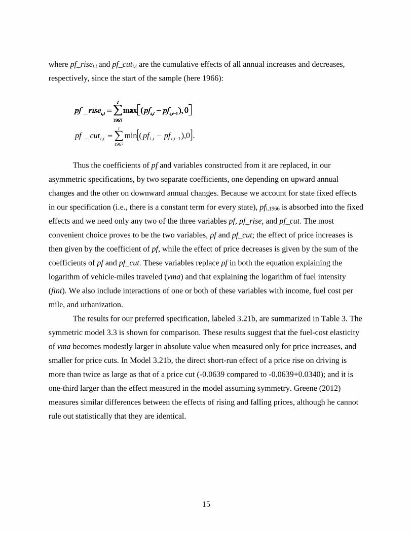
where pf_risei,t and pf_cuti,t are the cumulative effects of all annual increases and decreases,

respectively, since the start of the sample (here 1966):

[ ]. 0),(min_1967

1,,, ∑ −−=t

tititi pfpfcutpf

Thus the coefficients of pf and variables constructed from it are replaced, in our

asymmetric specifications, by two separate coefficients, one depending on upward annual

changes and the other on downward annual changes. Because we account for state fixed effects

in our specification (i.e., there is a constant term for every state), pfi,1966 is absorbed into the fixed

effects and we need only any two of the three variables pf, pf_rise, and pf_cut. The most

convenient choice proves to be the two variables, pf and pf_cut; the effect of price increases is

then given by the coefficient of pf, while the effect of price decreases is given by the sum of the

coefficients of pf and pf_cut. These variables replace pf in both the equation explaining the

logarithm of vehicle-miles traveled (vma) and that explaining the logarithm of fuel intensity

(fint). We also include interactions of one or both of these variables with income, fuel cost per

mile, and urbanization.

The results for our preferred specification, labeled 3.21b, are summarized in Table 3. The

symmetric model 3.3 is shown for comparison. These results suggest that the fuel-cost elasticity

of vma becomes modestly larger in absolute value when measured only for price increases, and

smaller for price cuts. In Model 3.21b, the direct short-run effect of a price rise on driving is

more than twice as large as that of a price cut (-0.0639 compared to -0.0639+0.0340); and it is

one-third larger than the effect measured in the model assuming symmetry. Greene (2012)

measures similar differences between the effects of rising and falling prices, although he cannot

rule out statistically that they are identical.

15

Table 3. Selected coefficient estimates: base model and asymmetric model (three-equation models)

Equation and variable: Coeff. Std. Error Coeff. Std. Errorvma equation:

pm=pf+fint -0.0466 0.0029 -0.0639 0.0049pf_cut +fint 0.0340 0.0078

pm*inc 0.0528 0.0108 0.0577 0.0108pm 2 -0.0124 0.0059 -0.0207 0.0061pm*Urban 0.0119 0.0094 0.0131 0.0093vma lagged 0.8346 0.0102 0.8334 0.0105

fint equation:pf +vma -0.0050 0.0041 -0.0097 0.0060

pf_cut +vma 0.0143 0.0123

Model 3.3 Model 3.21b

In the asymmetric model just described (3.21b), a change in fuel efficiency, unlike a

change in fuel price, has the same impact on vma regardless of whether fuel efficiency is

increased or decreased. Furthermore, the model posits that an increase in fuel efficiency has the

same impact (in percentage terms) as that of a fuel price cut. This makes sense from a theoretical

standpoint because most of the changes in fuel efficiency we are interested in are improvements,

i.e. they lower the fuel cost per mile just like price cuts. Furthermore, the pathways by which

consumers consider fuel efficiency are quite different from those by which they consider fuel

prices, so whatever is causing asymmetry need not affect both parts of fuel cost in the same

way.19

The estimated coefficients of the interaction terms from Model 3.21b are similar to those

from Model 3.3; the rebound effect increases with fuel price and decreases with income. But in

the asymmetric model, the coefficient on pm2 is larger in magnitude than in the model without

asymmetry. 20 21

19 Nevertheless, from a purely empirical point of view, the specification is arbitrary in that we could equally easily have used the variable pf_cut instead of pf_cut+fint—that is, we could have assumed that a change in fuel efficiency is viewed like a rise in price, not like a fall in price. Ideally we would include both variables, but this would effectively amount to measuring separate elasticities on pm and fint which, as explained in Section 3.2, our data seem mostly incapable of distinguishing.

20 We find very similar behavior if the unemployment rate is included in both the vma and fint equations, just as in Model 3.3c (as described at the end of Section 3.2). This model is reported in Appendix B as Model 3.21c. Just as with Model 3.3c, this model is superior in that it exhibits the expected effect of fuel price on desired fuel efficiency, in the form of a statistically significant coefficient for pf+vma in the fint equation. Nevertheless, this improvement makes essentially no difference to the results discussed in this paper.

16

We also estimated Model 3.21b using the generalized method of moments estimator

(GMM) instead of three stage least squares (3SLS). One drawback of the 3SLS estimator is the

difficulty involved in calculating clustered standard errors for a model as complex as 3.21b. If

there is indeed correlation in the standard errors within an individual state across years, the usual

standard errors are not consistent. We can, however, calculate standard errors clustered at the

state level for our primary model (3.21b) by using the GMM estimator if we omit the time trend

variables. Doing so also enables us to compare results across these two types of estimators.

Table 4 shows select results for three versions of model 3.21b; the left column uses 3SLS

as before, the middle column uses 3SLS but drops the time trend variable, and the right column

uses GMM without the time trend variable. The GMM point estimates and standard errors are

similar to those obtained from the 3SLS estimator, although the estimated coefficients for the

variables used to calculate the rebound effect are smaller in magnitude. Some of the difference in

those estimates is a result of excluding the time trend variable while some is attributable to the

change in estimator. Nevertheless, the GMM results are more or less consistent with the results

for alternate model specifications presented below. Finally, clustering the standard errors at the

state level changes the standard errors of coefficients very little, and does not change the

statistical significance of any of the variables in the model.

21 We also estimated a model analogous to 3.21b that included the fuel price variables measured in nominal rather than real dollars; we thank Stuart Rosenthal for this suggestion. The motivation for this model was the possibility that nominal price changes are more noticeable to drivers than real changes. The results, however, showed only a small and non-significant difference between drivers' responses to fuel price rises and cuts. This finding lends support to our primary asymmetric models and suggests that drivers are most responsive when fuel prices rise faster than inflation.

17

Table 4. Alternate estimators: selected coefficients from the vma equation.

The asymmetric model implies a somewhat different history of the stringency of the

CAFE standards than does our base model. This is because the asymmetric model implies that

price cuts and price rises enter separately as explanatory variables in the counter-factual

regression explaining fuel efficiency pre-1978, and their different coefficients are carried through

in projecting desired fuel efficiency post-1978. Figure 1 shows the variable cafe which, as

explained earlier, captures the difference between desired fuel efficiency and that mandated

under CAFE standards. Using the symmetric model to derive the desired fuel economy, the

stringency of CAFE standards drops to zero in 1995 and remains there. Using the asymmetric

Model 3.21b, however, the standards remain binding until 2006, with stringency jumping notably

upward in 2000 due to the sharp rise in fuel price during that year.

Figure 1. Stringency of CAFE standards

0.00

0.05

0.10

0.15

0.20

0.25

0.30

0.35

1965 1970 1975 1980 1985 1990 1995 2000 2005 2010

Varia

ble

cafe

p

Model 3.21b

Model 3.3

18

An alternative view of how asymmetry might work is that the difference in response

between fuel price rises or cuts is not so much in the magnitude, but in the speed with which the

response occurs. All the models considered in this paper already have an “inertia” built into

them, in the form of a lagged dependent variable which governs the speed of response to all

variable changes. But in Model 3.29b in Table 5, we allow also for the possibility that the speed

of the response differs between rises and cuts in fuel price. This is done by adding various lags of

pf_rise and pf_cut.

Table 5 Selected coefficient estimates: asymmetry in response to fuel price

The results suggest that adjustment to price rises takes place quickly; the response

elasticity is large in the year of and the first year following a price rise, then diminishes to a

smaller yet substantial value. But the adjustment to price cuts occurs more slowly: in absolute

value it is the smallest in the year of the change (0.140); takes its largest value after one year

(0.0626, from the sum of the first two coefficients between the dashed lines in Table 5); then

retreats to a value of 0.0215 (sum of all four coefficients) after three years. These response

19

patterns are shown in Figure 2.

Figure 2. Short-run elasticity of VMT with respect to a sustained change in fuel price (Model 3.29b)

-0.1000

-0.0800

-0.0600

-0.0400

-0.0200

0.0000

0.0200

0.0400

0.0600

0.0800

0 1 2 3

Year following change

Res

pons

e el

astic

ity

Rise in cost per mile Fall in cost per mile

3.3.2 Models based on rises versus falls of fuel cost

We also estimated models that base the asymmetry on the variable measuring fuel cost

per mile (pm), instead of on fuel price (pf). These models assume that people respond differently

depending on whether their fuel cost per mile is rising or falling, regardless of whether this is due

to a change in fuel price or in fuel efficiency. The variables used are formed analogously to the

previous subsection: fuel cost per mile, pm (the price of mileage), is decomposed into pm_rise

and pm_cut.

This decomposition raises a new problem because pm_rise and pm_cut are, like pm,

endogenous. In the symmetric model, endogeneity of pm is accounted for as part of the three-

20

equation model.22 But here the problem is worse: the values of these new variables in any given

year depend on values taken by an endogenous variable (fuel intensity) in previous years. A fully

endogenous treatment of pm_rise and pm_cut is thus not feasible, so we have used an

approximation: the variables are replaced by predicted values, pm_rise_hat and pm_cut_hat,

each of which is the value predicted by a regression of the corresponding variable on all the

exogenous variables in the system – that is, on the instruments in the 3SLS estimation routine.

This procedure basically replicates what instrumental variables does in the case of a simpler

endogenous variable, so the result of this approximation should be reasonably accurate although

the standard errors of these variables may be inaccurately measured.

Table 6 shows selected results of a specification, named Model 3.23, analogous to that of

Model 3.21b. The latter is shown for comparison. (Each model also contains three interaction

variables, whose coefficients are shown just below the dashed line.) The coefficient on

pm_cut_hat tells us the degree of asymmetry: it is positive, showing that the magnitude of the

elasticity is smaller for cost cuts than for cost rises. The short-run rebound effect is given by

elasticity -0.0623 when per-mile fuel costs are rising, and -0.0339 (=-0.0623+0.0284) when costs

are falling. The rebound effect is influenced by pm, income, and Urban much as before.

22 Formally, this is accomplished by entering the variable pm as the sum of two variables, pf + fint, where fint is the logarithm of fuel intensity (see Section 3, “Dependent variables”, definition of 1/E). Since fint is the dependent variable of the third equation of our model system, the simultaneous estimation performed by the three-stage least squares procedure treats it as endogenous where it enters the first equation as part of pm.

21

Table 6 Selected coefficient estimates: asymmetry in response to fuel price or fuel cost per mile

Equation and variable: Coeff. Std. Error Coeff. Std. Error

vma equation:pm= pf+ fint -0.0639 0.0049 -0.0623 0.0055

pf_cut + fint 0.0340 0.0078pm_cut_hat 0.0284 0.0093

pm*inc 0.0577 0.0107 0.0535 0.0112

pm2 -0.0207 0.0061 -0.0180 0.0062pm*Urban 0.0131 0.0093 0.0187 0.0099vma lagged 0.8334 0.0104 0.8084 0.0122

fint equation:pf + vma -0.0097 0.0060

pfrise -0.0133 0.0062pf_cut + vma 0.0143 0.0123pf_cut 0.0042 0.0096vma 0.0107 0.0166

Model 3.21b Model 3.23

In model 3.23, unlike those in the previous subsection, the response to a change in fuel

efficiency depends on what’s happening to overall fuel costs. If fuel price is rising more rapidly

than fuel efficiency, then these models predict that people would still respond to a small change

in fuel efficiency according to the combination of coefficients multiplying variable pm—that is,

they respond as they would to a rise in fuel price, even if they are actually responding to a fall in

fuel cost per mile. The behavioral rationale is as follows: if fuel costs are rising due to increasing

fuel prices and this has heightened people’s awareness, then an improvement in fuel efficiency

would have a large effect on their driving decisions because it would help offset that fuel price

rise at a time when they are highly sensitive to it. This is a debatable assumption, as it implies a

degree of rationality in calculating fuel costs that people may not have in reality.23 For this

reason, we prefer the models of Section 3.3.1.

23 For example, Larrick and Soll (2008) find that consumers have difficulty calculating the impact of fuel economy changes on fuel consumption when fuel economy is measured in miles per gallon. The authors refer to this phenomenon as the “MPG Illusion”.

22

3.4 Media attention and expectations

Two important findings of previous sections are that the responsiveness of vehicle travel

to costs sharply increased starting around 2003, and that this responsiveness is much larger when

fuel prices or costs are rising than when they are falling. But why? In this section, we consider

two factors that may help explain these variations in responsiveness.

The first is variations in media attention to fuel prices and costs. Motor vehicle fuel is a

moderately important part of many people’s budgets, and crude oil even more so. As a result,

there is a tendency for turmoil in gasoline or oil markets to gain much attention in public media.

The second is volatility in fuel costs. Volatility could cause consumers to adopt

contingency plans and thus pay more attention to fuel prices, even without help from the media.

On the other hand, consumers could ignore what they think are temporary price fluctuations; for

example, although consumers’ most common expectation of future prices is the current price,

under some circumstances they apparently expect some reversion to previous price levels.24

Data Description

We construct measures of media coverage based upon gas-price-related articles appearing

in the New York Times newspaper. Using the Proquest historical database , we tally the annual

number of article titles containing the words gasoline (or gas) and price (or cost). We then form

a variable equal to the annual fraction of all New York Times articles that are gas-price-related.

This fraction ranged from roughly 1/4000 during the 1960s to a high of 1/500 in 1974. Its

logarithm, normalized by subtracting its mean, is shown in Figure 3. In the specifications shown

here, we use a dummy variable Media_dummy equal to one when the ratio exceeds its 1996-2009

median value.25

24 Supporting evidence comes from two separate surveys, reported by Anderson et al. (2011) and Allcott (2011), both of which asked people directly about their price expectations. Anderson et al. (2011) find that a random walk assumption accurately explains their answers except in late 2008, when people expected (correctly, as it turned out) that the recent fall in prices would prove to be temporary.

25Media_dummy is equal to one in years 1973-1981, 1983, 1990-1992, 1994-1997, 2000, 2004-2006, and 2008. It is not normalized.

23

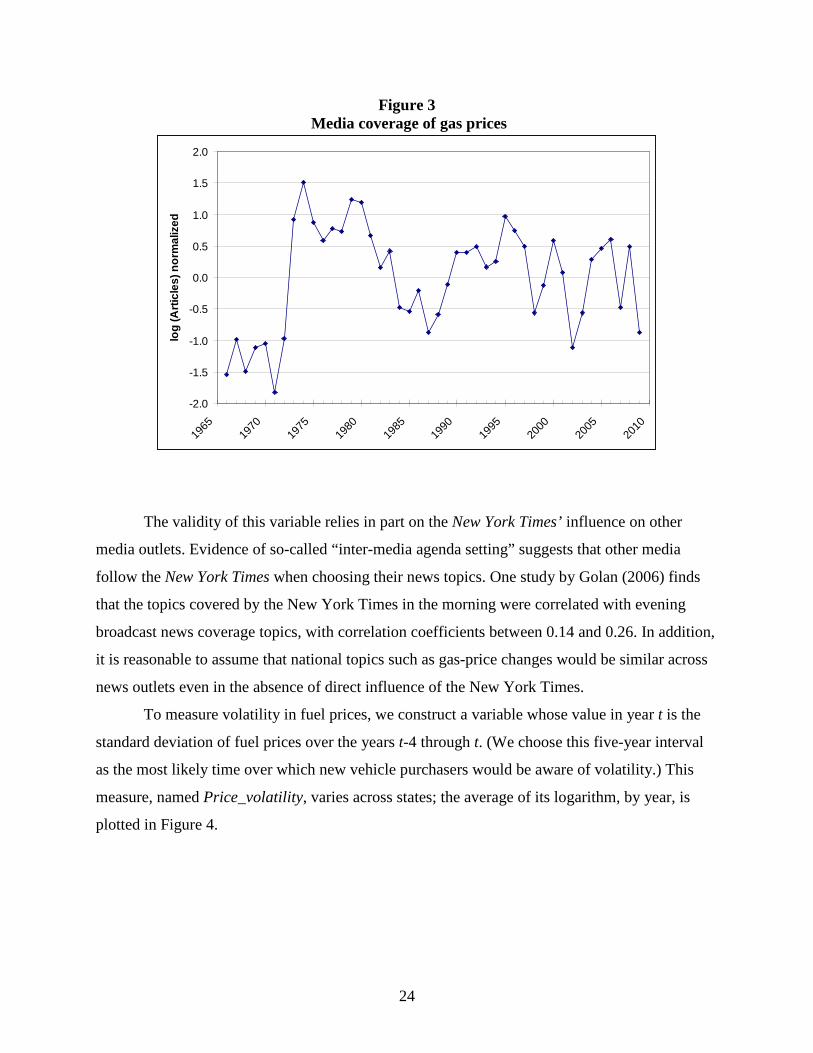
Figure 3 Media coverage of gas prices

-2.0

-1.5

-1.0

-0.5

0.0

0.5

1.0

1.5

2.0

1965

1970

1975

1980

1985

1990

1995

2000

2005

2010

log

(Arti

cles

) nor

mal

ized

The validity of this variable relies in part on the New York Times’ influence on other

media outlets. Evidence of so-called “inter-media agenda setting” suggests that other media

follow the New York Times when choosing their news topics. One study by Golan (2006) finds

that the topics covered by the New York Times in the morning were correlated with evening

broadcast news coverage topics, with correlation coefficients between 0.14 and 0.26. In addition,

it is reasonable to assume that national topics such as gas-price changes would be similar across

news outlets even in the absence of direct influence of the New York Times.

To measure volatility in fuel prices, we construct a variable whose value in year t is the

standard deviation of fuel prices over the years t-4 through t. (We choose this five-year interval

as the most likely time over which new vehicle purchasers would be aware of volatility.) This

measure, named Price_volatility, varies across states; the average of its logarithm, by year, is

plotted in Figure 4.

24

Figure 4 Fuel price volatility

0

5

10

15

20

25

1965 1975 1985 1995 2005

avg

log

std

dev

fuel

pric

e

Specification and results

Table 7 shows several models which include the one or both of the variables for media

coverage and price volatility, each interacted with either fuel price or fuel cost.26 The media

variable is specified to influence the response to fuel price but not to fuel efficiency, because the

variable involves news about fuel prices; this is accomplished by interacting it with pf and not

pm. This implies that media coverage impacts the rebound elasticity only indirectly, via changes

in estimated coefficients. The volatility variable, by contrast, reflects a consumer’s own

experience with variation in fuel costs, and therefore we specify it so as to influence the response

to both price and fuel efficiency (i.e., it is interacted with pm rather than pf). For comparison, the

table also shows two models incorporating asymmetry but not media or uncertainty (Models

3.21b and 3.21d).

26 As with other interacting variables, we normalize each variable by subtracting its mean value on the entire sample; this is done for convenience so that the coefficient of pf or pm measures the short-run structural VMT elasticity when all interacting variables take their mean values in the sample.

25

Table 7 Selected coefficient estimates: asymmetry with media coverage

and/or fuel-price uncertainty

Equation and Variable Coeff. Std. Error Coeff. Std.

Error Coeff. Std. Error Coeff. Std.

Error Coeff. Std. Error

vma equation:pm = pf + fint -0.0639 0.0049 -0.0710 0.0052 -0.0587 0.0052 -0.0325 0.0088 -0.0351 0.0097

pf_cut + fint 0.0340 0.0078 0.0394 0.0080 0.0286 0.0081 0.0242 0.0089 0.0246 0.0092pm * Dummy_0309 -0.0277 0.0076 -0.0144 0.0086pf * Media_dummy -0.0301 0.0101 -0.0412 0.0102 -0.0443 0.0105pm * Price_volatility -0.0018 0.0005 -0.0011 0.0005pm * inc 0.0577 0.0107 0.0759 0.0122 0.0583 0.0109 0.0620 0.0113 0.0671 0.0131

pm 2 -0.0207 0.0061 -0.0216 0.0061 -0.0053 0.0075 0.0204 0.0100 0.0107 0.0105pm * Urban 0.0131 0.0093 0.0099 0.0094 0.0118 0.0094 0.0025 0.0099 0.0056 0.0102vma lagged 0.8334 0.0104 0.8265 0.0106 0.8325 0.0106 0.8439 0.0108 0.8397 0.0115

fint equation:pf + vma -0.0097 0.0060 -0.0078 0.0059 -0.0124 0.0059 -0.0109 0.0058 -0.0093 0.0058pf_cut + vma 0.0143 0.0123 0.0069 0.0120 0.0220 0.0120 0.0210 0.0119 0.0120 0.0117

Model 3.55dModel 3.55Model 3.21b Model 3.21d Model 3.35

Models 3.35 and 3.55 show that both media coverage and price volatility exert strong

influences on the price-elasticity of motor vehicle travel, increasing the response to fuel price

changes and, in the case of volatility, to fuel efficiency changes as well.27 In fact, the effect of

price volatility is so strong as to eliminate the previously observed positive effect of fuel cost

itself on the magnitude of the rebound elasticity: the coefficient of pm2 is now reversed in sign

and just barely statistically significant. This suggests that the rise in the magnitude of the

elasticity of VMT during the 2000s was due more to volatility than to the higher level of fuel

price.28

Because we specified the media variable to interact with fuel price but volatility to

27 The base response (coefficient of pm is negative, so a negative coefficient on an interaction term mean the magnitude of the response increases with the interacting variable. Because these variables are multiplied by pf or by pm≡pf+fint, and because pf≡pf_fire+pf_cut, the coefficients of the interactions are part of both ∂vma/∂pf_rise and ∂vma/∂pf_cut. The coefficient of pf_cut indicates a wedge between the response to price rises and price cuts, a wedge whose size does not depend on the media or volatility variable.

28 These same characteristics persist in the presence of a variable measuring unemployment, and if additional lags are added as with Model 3.29b. (The effects of those additional lags show the same pattern, and nearly the same magnitudes, as in Model 3.29b.)

26

interact with fuel cost, the “rebound effect,” defined as the response to changes in fuel efficiency,

is increased in magnitude by fuel-price volatility but not by media coverage. To put it differently,

given the assumptions of the specification, we find that media coverage tends to intensify the

effect of fuel prices, while fuel price volatility intensifies the effect of per mile fuel costs

whatever their source. Furthermore, media coverage undoubtedly responds to consumer interest

and therefore could be correlated with other variables affecting VMT, thus making it endogenous

and limiting its usefulness for drawing policy implications.

We noted earlier the appearance of a shift in the structural elasticity toward higher values

during the period 2003-09. Model 3.21d confirms that this shift exists even in models with

asymmetric responses.29 Model 3.55d reveals, however, that about half this shift can be

explained by our media and volatility variables. (Other models, not shown, demonstrate that

those two variables share approximately equally in this task of explaining the shift.) The

remainder of the shift (1.44 percentage points of elasticity) is still unexplained, leaving room for

future research to uncover the missing factors.

For completeness, Table 8 shows the long-run price elasticities of VMT, fuel efficiency,

and fuel consumption using our most preferred models. The elasticities are calculated using

equations (5) and their counterparts as described by Small and Van Dender (2007). The full

estimation results for these three models are listed in Appendix B.2.

29 The variable Dummy_0309 is equal to one for years 2003-2009 and zero otherwise, except here it has been normalized (like other variables interacted with pm) by subtracting its mean, which is 7/44 = 0.159. (In Model 3.18, it was not normalized.)

27

Table 8. Long-run elasticities implied by preferred models Model 3.3

Elasticities:Price rising

Price falling

Price rising

Price falling

VMT with respect to fuel efficiency: At sample averagea -0.295 -0.184 -0.184 -0.052 -0.052 At US 2000-2009 avg.b -0.178 -0.042 -0.042 -0.040 -0.040VMT with respect to fuel price: At sample averagea -0.295 -0.397 -0.184 -0.214 -0.052 At US 2000-2009 avg.b -0.178 -0.255 -0.042 -0.202 -0.040

Fuel consumption with respect to fuel price: At sample averagea -0.322 -0.433 -0.249 -0.279 -0.146 At US 2000-2009 avg.b -0.213 -0.309 -0.130 -0.269 -0.136

Notes:

Model 3.55

aElasticities measured at sample average values of pm , inc , & Urban for years 1966-2009.bElasticities measured at sample average values of pm , inc , & Urban for years 2000-2009.

Model 3.21b

4. Conclusion

The research reported here, extending Small and Van Dender (2007) with data through

2009, confirms the findings of previous studies that the long-run rebound effect, measured over a

period of several decades extending back to 1966, is close to 30%. We also find a short-run (one-

year) rebound effect, again averaged over that entire period, of about 4.7%.

Furthermore, we confirm earlier findings that the rebound effect became substantially

smaller in magnitude over the course of that time period, probably due to a combination of

higher real incomes, lower real fuel costs, and higher urbanization. Our base model (Model 3.3)

implies that the long-run rebound effect is 17.8% when evaluated at average values of income,

fuel cost, and urbanization over the years 2000-2009.

We also report some new findings. There is strong evidence of asymmetry in

responsiveness to price increases and decreases. This makes interpretation of the rebound effect

more difficult, because it accentuates the unresolved question as to whether travelers respond to

a change in fuel efficiency in the same way as to a change in fuel price.

In both symmetric and asymmetric response models, there is an upward shift in the

rebound effect, of 2.5 to 2.8 percentage points, starting in 2003. We introduce two new variables,

28

which together explain about half of this shift. The first is media coverage of fuel prices; the

second is fuel-price volatility. Both substantially increase travelers’ responsiveness to changes in

fuel price and/or fuel cost. Nevertheless, these influences are small enough in magnitude that

they do not fully offset the downward trend in VMT response elasticities due to higher incomes

and other factors. Hence even assuming the variables retain their 2000-2009 values into the

indefinite future, they would not prevent a further diminishing of the magnitude of the rebound

effect if incomes continue to grow at anything like historic rates.

29

References

Allcott, Hunt (2011), “Consumers’ Perceptions and Misperceptions of Energy Costs,” American Economics Review: Papers and Proceedings, 101(3): 98-104. Anderson, Soren T., Ryan Kellogg, James M. Sallee, and Richard T. Curtin (2011), “Forecasting Gasoline Prices Using Consumer Surveys,” American Economic Review: Papers and Proceedings, 101(3), 110-114.

Borenstein, Severin (2013), “A Microeconomic Framework for Evaluating Energy Efficiency Rebound and Some Implications,” Working paper 19044, National Bureau of Economics Research, May.

Brons, Martijn, Peter Nijkamp, Eric Pels, and Piet Rietveld (2008), “A meta-analysis of the price elasticity of gasoline demand: A SUR approach,” Energy Economics, 30: 2105-2122.

Dargay, J., 2007. The effect of prices and income on car travel in the UK. Transportation Research Part A: Policy and Practice, 41(10), 949-960.Davis, Stacy C., Susan W. Diegel, and Robert G. Boundy (2011), Transportation Energy Data Book, 30th edition, Oak Ridge National Laboratory, June. http://cta.ornl.gov/data/index.shtml

Dargay, Joyce M., and Dermot Gately, 1997, "The Demand for Transportation Fuels: Imperfect Price-reversibility?" Transportation Research – Part B, 31(1):71-82.

Dargay, Joyce M., Dermot Gately, and Martin Sommer (2007), “Vehicle Ownership and Income Growth, Worldwide: 1960-2030. Energy Journal, 28(4): 143-170.

Gately, Dermot, and Hillard G. Huntington, 2002. "The Asymmetric Effects of Changes in Price and Income on Energy and Oil Demand" Energy Journal, 23(1), pp. 19-55.

Gillingham, Kenneth (2011), The Consumer Response to Gasoline Price Changes: Empirical Evidence and Policy Implications. Ph.D. Dissertation, Dept. of Management Science and Engineering, Stanford University, June. http://purl.stanford.edu/wz808zn3318

Gillingham, Kenneth (2013), “Identifying the Elasticity of Driving: Evidence from a Gasoline Price Shock in California,” working paper, Yale University, February.http://www.yale.edu/gillingham/Gillingham_IdentifyingElasticityDriving.pdf

Golan, Guy (2006), Inter-Media Agenda Setting and Global News Coverage: Assessing the influence of the New York Times on three network television evening news programs,” Journalism Studies, 7(2), 323-333.

Goodwin, P., J. Dargay, and M. Hanly (2004). “Elasticities of Road Traffic and Fuel Consumption with Respect to Price and Income: A Review,” Transport Reviews, 24 (3), 275-292.

Graham, D.J., Glaister, S., 2004, Road traffic demand elasticity estimates: a review. Transport Reviews, 24(3), 261-274.

30

Greene, D.L. (1992). “Vehicle Use and Fuel Economy: How Big is the Rebound Effect?” Energy Journal, 13 (1), 117-143.

Greene, David L. (2012), “Rebound 2007: Analysis of U.S. Light-Duty Vehicle Travel Statistics,” Energy Policy, 41: 14–28.

Greene D.L., J.R. Kahn and R.C. Gibson (1999). “Fuel Economy Rebound Effect for US Households, Energy Journal, 20 (3), 1-31.

Greening, L.A., D.L. Greene and C. Difiglio (2000). “Energy Efficiency and Consumption – The Rebound Effect – A Survey,” Energy Policy, 28, 389-401.

Haughton, J. and S. Sarkar (1996). “Gasoline Tax as a Corrective tax: Estimates for the United States (1970-1991),” Energy Journal, 17 (2), 103-126.

Hughes, Jonathan E., Christopher R. Knittel, and Daniel Sperling (2008), “Evidence of a Shift in the Short-Run Price Elasticity of Gasoline Demand,” Energy Journal, 29(1): 113-134.

Hymel, Kent, Kenneth A. Small, and Kurt Van Dender (2010). “Induced Demand and Rebound Effects in Road Transport,” Transportation Research Part B – Methodological, 44(10), 1220-1241.

Knittel, Christopher R., and Ryan Sandler (2012), “Carbon Prices and Greenhouse Gas Emissions: The Intensive and Extensive Margins,” in Don Fullerton and Catherine Wolfram, eds., Design and Implementation of U.S. Climate Policy, University of Chicago Press, ch. 18, pp. 287-299.

Knittel, Christopher R., and Ryan Sandler (2013), “The Welfare Impact of Indirect Pigouvian Taxation: Evidence from Transportation,” Working Paper 18849, National Bureau of Economic Research. http://www.nber.org/papers/w18849

Jones C.T. (1993). “Another Look at U.S. Passenger Vehicle Use and the ‘Rebound’ Effect from Improved Fuel Efficiency,” Energy Journal, 14 (4), 99-110.

Litman, Todd (2013), “Changing North American vehicle travel price sensitivities: Implications for transport and energy policy,” Transport Policy, 28: 2-10.

Mackie P.J., A.S. Fowkes, M. Wardman, G. Whelan, J. Nellthorp, and J. Bates (2003) Values of Travel Time Savings in the UK: Summary Report, report to the UK Department for Transport. Leeds, UK: Institute of Transport Studies, Univ. of Leeds. http://www.dft.gov.uk/pgr/economics/rdg/valueoftraveltimesavingsinth3130?page=1#a1000

Molloy, Raven, and Hui Shan (2013), “The effect of gasoline prices on household location,” Review of Economics and Statistics 95(4): 1212–1221.

NHTSA (National Highway Traffic Safety Administration) (2012), Corporate Average Fuel Economy for MY 2017-MY 2025 Passenger Cars and Light Trucks: Final Regulatory Impact Analysis, August. www.nhtsa.gov/staticfiles/rulemaking/pdf/cafe/FRIA_2017-2025.pdf Schrank, David, Tim Lomax, and Shawn Turner (2010). Urban Mobility Report 2010, Texas Transportation Institute, December. http://mobility.tamu.edu

31

Small K.A. and K. Hymel (2013), The Rebound Effect from Fuel Efficiency Standards: Measurement and Projection to 2035, Final report to U.S. Environmental Protection Agency, contract EP-W-08-018, March 26.

Small K.A. and K. Van Dender (2007). “Fuel Efficiency and Motor Vehicle Travel: The Declining Rebound Effect,” Energy Journal 28: 25-51.

Small K.A. and E.T. Verhoef (2007) The Economics of Urban Transportation, London and New York: Routledge, forthcoming.

Wadud Z., D.J. Graham, and R.B. Noland (2007a). “Gasoline demand with heterogeneity in household responses,” Working paper, Centre for Transport Studies, Imperial College London.

Wadud Z., D.J. Graham, and R.B. Noland (2007b). “Modelling fuel demand for different socio-economic groups,” Working paper, Centre for Transport Studies, Imperial College London.

West, Sarah E. (2004), “Distributional effects of alternative vehicle pollution control policies,” Journal of Public Economic, 88: 735-757.

32

Appendix A. Data

A.1 Variables used

Variables used in our base model are described below. For data sources, see Small and Van

Dender (2007b) and Hymel et al. (2010).

Dependent Variables M: Vehicle miles traveled (VMT) divided by adult population, by state and year (logarithm:

vma, for “vehicle-miles per adult”). V: Vehicle stock divided by adult population (logarithm: vehstock). 1/E: Fuel intensity, measured as F/M, where F is highway use of gasoline30 (logarithm: fint). C: Total hours of congestion delay in the state divided by adult population (logarithm: cong).

See Section 3.1 for further details

Independent Variables other than CAFE PM: Fuel cost per mile, PF/E. Its logarithm is denoted pm ≡ ln(PF)–ln(E) ≡ pf+fint. For

convenience in interpreting interaction variables based on pm, we have normalized it by subtracting its mean over the sample.

PV: Index of real new vehicle prices (1987=100) (logarithm: pv). 31 PF: Price of gasoline, deflated by consumer price index (1987=1.00) (cents per gallon).

Variable pf is its logarithm normalized by subtracting the sample mean. Other: See Small and Van Dender (2007b), Appendix A; and Small, Hymel, and Van Dender

(2010), Appendices A and B. The first three equations include time trends to proxy for unmeasured trends such as residential dispersion, other driving costs, lifestyle changes, and technology. As described below, in equation (8), the set of variables denoted XM includes the variable (pm)2 and interactions between normalized pm and other normalized variables: log real per capita income (inc), and fraction urbanized (Urban – used only in the three-equation model) and normalized cong (used only in the four-equation model).

30 This term is used by FHWA to mean use by vehicles traveling on public roadways of all types. It excludes use by not licensed for roadways, such as construction equipment and farm vehicles.

31 We include new-car prices in the second equation as indicators of the capital cost of owning a car. We exclude used-car prices because they are likely to be endogenous; also reliable data by state are unavailable.

A-1

A.2 Adjustments to State population data

Several variables specification, including all but one of the endogenous variables, make

use of data on adult or total state population as a divisor. Such data are published by the U.S.

Census Bureau as midyear population estimates; they use demographic information at the state

level to update the most recent census count, taken in years ending with zero. However, these

estimates do not always match the subsequent census count, and the Census Bureau does not

update them to create a consistent series. As a result, the published series contains many

instances of implausible jumps in the years of the census count. In both of our earlier published

papers, we applied a correction assuming that the actual census counts taken every ten years are

accurate, and that the error in estimating population between them grows linearly over that ten-

year time interval. This approach is better than using the published estimates because it makes

use of Census year data that were not available at the time the published estimates were

constructed (namely, data from the subsequent census count). See Small and Van Dender

(2007b) for details.

For this paper, the same procedure was applied to the 2001-2009 data using Census

counts for 2010. This adjustment was not made for the post-2000 data in the earlier papers due to

unavailability at that time of the 2010 Census counts.

Additional references Small K.A. and K. Van Dender (2007b). “Fuel Efficiency and Motor Vehicle Travel: The Declining Rebound Effect,” Working Paper No. 05-06-03, Department of Economics, University of California at Irvine (revised).

A-2

Appendix B. Additional estimation results B.1 Models including unemployment rate: selected results

Table B1. Three-equation models with and without unemployment variables

Equation and variable: Coeff. Std. Error

Coeff. Std. Error

Coeff. Std. Error

Coeff. Std. Error

Coeff. Std. Error

Coeff. Std. Error

vma equation:pm= pf+ fint -0.0466 0.0029 -0.0416 0.0038 -0.0464 0.0029 -0.0429 0.0031 -0.0639 0.0049 -0.0601 0.0052

pf_cut + fint 0.0340 0.0078 0.0302 0.0079pm*dummy_0309 -0.0251 0.0076 -0.0230 0.0079pf * (Media_dummy )pm* log(varpf )

pm*inc 0.0528 0.0108 0.0521 0.0110 0.0699 0.0121 0.0694 0.0122 0.0577 0.0107 0.0620 0.0107pm2 -0.0124 0.0059 -0.0176 0.0060 -0.0113 0.0060 -0.0148 0.0060 -0.0207 0.0061 -0.0242 0.0061pm*Urban 0.0119 0.0094 0.0142 0.0098 0.0078 0.0096 0.0075 0.0097 0.0131 0.0093 0.0117 0.0093Unemployment rate -0.0015 0.0005 -0.0017 0.0005 -0.0011 0.0005vma lagged 0.8346 0.0102 0.8380 0.0104 0.8279 0.0105 0.8306 0.0106 0.8334 0.0104 0.8348 0.0104

veh equationUnemployment rate -0.0029 0.0007 -0.0029 0.0007 -0.0028 0.0007

fint equation:pf + vma -0.0050 0.0041 -0.0143 0.0043 -0.0052 0.0041 -0.0140 0.0043 -0.0097 0.0060 -0.0308 0.0070

pf_cut + vmaUnemployment rate 0.0047 0.0007 0.0043 0.0007 0.0056 0.0008

Model 3.21b Model 3.21cModel 3.3 Model 3.3c Model 3.18 Model 3.18c

A-1

B.2 Full estimation results for preferred models

Table B2 Full estimation results for preferred models

Equation Variable Coeff. Std. Err. Coeff. Std. Err. Coeff. Std. Err.vma intercept 1.6261 0.1022 3.1468 0.3541 2.6249 0.4077vma inc 0.0781 0.0117 0.0770 0.0118 0.0667 0.0129vma Adults / road mile -0.0149 0.0038 -0.0151 0.0037 -0.0133 0.0039vma popratio 0.0726 0.0322 0.0630 0.0323 -0.0024 0.0364vma Urban -0.0205 0.0391 -0.0061 0.0395 -0.0122 0.0406vma Railpop -0.0067 0.0043 -0.0082 0.0042 -0.0075 0.0044vma D7479 -0.0439 0.0034 -0.0445 0.0035 -0.0490 0.0038vma Trend -0.0004 0.0002 0.0013 0.0004 0.0011 0.0005vma vma(-1) 0.8346 0.0102 0.8334 0.0104 0.8439 0.0108vma vehstock 0.0209 0.0067 0.0161 0.0067 0.0142 0.0069vma pm = pf + fint -0.0466 0.0029 -0.0639 0.0049 -0.0325 0.0088vma pm^2 -0.0124 0.0059 -0.0207 0.0061 0.0204 0.0100vma pm*inc 0.0528 0.0108 0.0577 0.0107 0.0620 0.0113vma pm*Urban 0.0119 0.0094 0.0131 0.0093 0.0025 0.0099vma pfcut + fint 0.0340 0.0078 0.0242 0.0089vma pf*Media_dummy -0.0412 0.0102vma pm*Price_volatility -0.0018 0.0005vma AR(1) -0.1018 0.0204 -0.1021 0.0204 -0.1012 0.0208vma State fixed effects yes yes yesveh intercept -0.2253 0.1452 -0.2188 0.1449 -0.2206 0.1448veh pnewcar 0.0400 0.0317 0.0460 0.0317 0.0458 0.0317veh interest -0.0008 0.0042 -0.0004 0.0042 -0.0006 0.0042veh income 0.0032 0.0146 0.0038 0.0146 0.0038 0.0146veh adults / road mile -0.0136 0.0060 -0.0137 0.0060 -0.0137 0.0060veh licenses/adult 0.0345 0.0184 0.0349 0.0183 0.0351 0.0183veh trend 0.0002 0.0007 0.0004 0.0007 0.0004 0.0007veh vehstock(-1) 0.9318 0.0104 0.9316 0.0104 0.9317 0.0104veh vma 0.0291 0.0147 0.0281 0.0146 0.0283 0.0146veh pm 0.0013 0.0058 0.0019 0.0058 0.0018 0.0058veh AR(1) -0.1461 0.0230 -0.1469 0.0230 -0.1467 0.0230veh State fixed effects yes yes yesfint intercept -0.2447 0.0631 0.9282 1.0517 1.4590 1.0132fint pf + vma -0.0050 0.0041 -0.0097 0.0060 -0.0109 0.0058fint inc -0.0016 0.0144 0.0000 0.0146 -0.0017 0.0144fint fint(-1) 0.9040 0.0100 0.8977 0.0115 0.8947 0.0115fint popratio -0.0168 0.0603 -0.0005 0.0586 0.0300 0.0600fint Trend66-73 0.0005 0.0011 -0.0005 0.0011 0.0001 0.0011fint Trend74-79 -0.0068 0.0010 -0.0061 0.0011 -0.0063 0.0011fint Trend80+ -0.0007 0.0003 -0.0002 0.0007 0.0002 0.0007fint D7479 -0.0070 0.0048 -0.0032 0.0048 -0.0022 0.0048fint Urban -0.0905 0.0467 -0.0890 0.0471 -0.0863 0.0467fint cafe -0.0345 0.0108 -0.0256 0.0183 -0.0103 0.0171fint pfcut + vma 0.0143 0.0123 0.0210 0.0119fint AR(1) -0.1773 0.0201 -0.1804 0.0202 -0.1858 0.0202fint State fixed effects yes yes yes

Model 3.3 Model 3.21b Model 3.55

A-2