the random feature model on function space

THE RANDOM FEATURE MODEL FOR INPUT-OUTPUT MAPSBETWEEN BANACH SPACES∗

NICHOLAS H. NELSEN† AND ANDREW M. STUART‡

Abstract. Well known to the machine learning community, the random feature model, originallyintroduced by Rahimi and Recht in 2008, is a parametric approximation to kernel interpolation orregression methods. It is typically used to approximate functions mapping a finite-dimensional inputspace to the real line. In this paper, we instead propose a methodology for use of the random featuremodel as a data-driven surrogate for operators that map an input Banach space to an output Banachspace. Although the methodology is quite general, we consider operators defined by partial differentialequations (PDEs); here, the inputs and outputs are themselves functions, with the input parametersbeing functions required to specify the problem, such as initial data or coefficients, and the outputsbeing solutions of the problem. Upon discretization, the model inherits several desirable attributesfrom this infinite-dimensional, function space viewpoint, including mesh-invariant approximationerror with respect to the true PDE solution map and the capability to be trained at one meshresolution and then deployed at different mesh resolutions. We view the random feature model asa non-intrusive data-driven emulator, provide a mathematical framework for its interpretation, anddemonstrate its ability to efficiently and accurately approximate the nonlinear parameter-to-solutionmaps of two prototypical PDEs arising in physical science and engineering applications: viscousBurgers’ equation and a variable coefficient elliptic equation.

Key words. random feature, surrogate model, emulator, parametric PDE, solution map, high-dimensional approximation, model reduction, supervised learning, data-driven scientific computing

AMS subject classifications. 65D15, 65D40, 62M45, 35R60

1. Introduction. The goal of this paper is to frame the random feature model,introduced in [57], as a methodology for the data-driven approximation of maps be-tween infinite-dimensional spaces. Canonical examples of such maps include the semi-group generated by a time-dependent partial differential equation (PDE) mapping theinitial condition (an input parameter) to the solution at a later time and the oper-ator mapping a coefficient function (an input parameter) appearing in a PDE toits solution. Obtaining efficient and potentially low-dimensional representations ofPDE solution maps is not only conceptually interesting, but also practically useful.Many applications in science and engineering require repeated evaluations of a com-plex and expensive forward model for different configurations of a system parameter.The model often represents a discretized PDE and the parameter, serving as inputto the model, often represents a high-dimensional discretized quantity such as an ini-tial condition or uncertain coefficient field. These outer loop applications commonlyarise in inverse problems or uncertainty quantification tasks that involve control, op-timization, or inference [56]. Full order forward models do not perform well in suchmany-query contexts, either due to excessive computational cost (requiring the mostpowerful high performance computing architectures) or slow evaluation time (unac-ceptable in real-time contexts such as on-the-fly optimal control). In contrast to the

∗Submitted to the editors May 20, 2020.Funding: NHN is supported by the National Science Foundation Graduate Research Fellowship

Program under award DGE-1745301. AMS is supported by NSF (award DMS-1818977) and by theOffice of Naval Research (award N00014-17-1-2079). Both authors are supported by NSF (awardAGS-1835860).†Mechanical and Civil Engineering, California Institute of Technology, Pasadena, CA 91125, USA

([email protected]).‡Computing and Mathematical Sciences, California Institute of Technology, Pasadena, CA 91125,

USA ([email protected]).

1

arX

iv:2

005.

1022

4v1

[m

ath.

NA

] 2

0 M

ay 2

020

mailto:[email protected]

mailto:[email protected]

2 N. H. NELSEN AND A. M. STUART

big data regime that dominates computer vision and other technological fields, onlya relatively small amount of high resolution data is generated from computer simula-tions or physical experiments in scientific applications. Fast approximate solvers builtfrom this limited available data that can efficiently and accurately emulate the fullorder model would be highly advantageous.

In this work, we demonstrate that the random feature model holds considerablepotential for such a purpose. Resembling [50] and the contemporaneous work in [11,48], we present a methodology for true function space learning of black-box input-output maps between a Banach space and separable Hilbert space. We formulate theapproximation problem as supervised learning in infinite dimensions and show thatthe natural hypothesis space is a reproducing kernel Hilbert space associated with anoperator-valued kernel. For a suitable loss functional, training the random featuremodel is equivalent to solving a finite-dimensional convex optimization problem. Asa consequence of our careful construction of the method as mapping between Banachspaces, the resulting emulator naturally scales favorably with respect to the high inputand output dimensions arising in practical, discretized applications; furthermore, itis shown to achieve small relative test error for two model problems arising fromapproximation of a semigroup and the solution map for an elliptic PDE exhibitingparametric dependence on a coefficient function.

1.1. Literature Review. In recent years, two different lines of research haveemerged that address PDE approximation problems with machine learning techniques.The first perspective takes a more traditional approach akin to point collocation meth-ods from the field of numerical analysis. Here, the goal is to use a deep neural network(NN) to solve a prescribed initial boundary value problem with as high accuracy aspossible. Given a point cloud in a spatio-temporal domain D as input data, the pre-vailing approach first directly parametrizes the PDE solution field as a NN and thenoptimizes the NN parameters by minimizing the PDE residual with respect to (w.r.t.)some loss functional (see [58, 64, 71] and the references therein). To clarify, the objectapproximated with this novel method is a low-dimensional input-output map D → R,i.e., the real-valued function that solves the PDE. This approach is mesh-free by def-inition but highly intrusive as it requires full knowledge of the specified PDE. Anychange to the original formulation of the initial boundary value problem or relatedPDE problem parameters necessitates an (expensive) re-training of the NN solution.We do not explore this first approach any further in this article.

The second direction is arguably more ambitious: use a NN as an emulator for theinfinite-dimensional mapping between an input parameter and the PDE solution itselfor a functional of the solution, i.e., a quantity of interest; the latter is widely prevalentin uncertainty quantification problems. We emphasize that the object approximatedin this setting, unlike in the aforementioned first approach, is an input-output mapX → Y, i.e., the PDE solution operator, where X , Y are infinite-dimensional Banachspaces; this map is generally nonlinear. For an approximation-theoretic treatmentof parametric PDEs in general, we refer the reader to the article of Cohen and De-Vore [19]. In applications, the solution operator is represented by a discretized forwardmodel RK → RK , where K is the mesh size, and hence represents a high-dimensionalobject. It is this second line of research that inspires our work.

Of course, there are many approaches to forward model reduction that do notexplicitly involve machine learning ideas. The reduced basis method (see [4, 7, 24]and the references therein) is a classical idea based on constructing an empirical basisfrom data snapshots and solving a cheaper variational problem; it is still widely used

THE RANDOM FEATURE MODEL ON FUNCTION SPACE 3

in practice due to computationally efficient offline-online decompositions that elim-inate dependence on the full order degrees of freedom. Recently, machine learningextensions to the reduced basis methodology, of both intrusive (e.g., projection-basedreduced order models) and non-intrusive (e.g., model-free data only) type, have fur-ther improved the applicability of these methods [17, 29, 37, 46, 62]. However, theinput-output maps considered in these works involve high dimension in only one ofthe input or output space, not both. Other popular surrogate modeling techniquesinclude Gaussian processes [74], polynomial chaos expansions [65], and radial basisfunctions [72]; yet, these are only practically suitable for problems with input space oflow to moderate dimension. Classical numerical methods for PDEs may also representthe forward model RK → RK , albeit implicitly in the form a computer code (e.g.:finite element, finite difference, finite volume methods). However, the approximationerror is sensitive to K and repeated evaluations of this forward model often becomescost prohibitive due to poor scaling with input dimension K.

Instead, deep NNs have been identified as strong candidate surrogate models forparametric PDE problems due to their empirical ability to emulate high-dimensionalnonlinear functions with minimal evaluation cost once trained. Early work in theuse of NNs to learn the solution operator, or vector field, defining ODEs and time-dependent PDEs, may be found in the 1990s [33, 59]. There are now more theo-retical justifications for NNs breaking the curse of dimensionality [45, 53], leadingto increased interest in PDE applications [30, 63]. A suite of work on data-drivendiscretizations of PDEs has emerged that allow for identification of the governingmodel [3, 12, 49, 67]; we note that only the operators appearing in the equation it-self are approximated with these approaches, not the solution operator of the PDE.More in line with our focus in this article, architectures based on deep convolutionalNNs have proven quite successful for learning elliptic PDE solution maps (for exam-ple, see [68, 75, 76], which take an image-to-image regression approach). Other NNshave been used in similar elliptic problems for quantity of interest prediction [43], errorestimation [15], or unsupervised learning [47]. Yet in all the approaches above, the ar-chitectures and resulting error are dependent on the mesh resolution. To circumventthis issue, the surrogate map must be well-defined on function space and indepen-dent of any finite-dimensional realization of the map that arises from discretization.This is not a new idea (see [16, 60] or for functional data analysis, [40, 54]). Theaforementioned reduced basis method is an example, as is the method of [18, 19],which approximates the solution map with sparse Taylor polynomials and is provedto achieve optimal convergence rates in idealized settings. However, it is only recentlythat machine learning methods have been explicitly designed to operate in an infinite-dimensional setting, and there is little work in this direction [11, 48]. Here we proposethe random feature model as another such method.

The random feature model (RFM) [57], detailed in Subsection 2.3, is in somesense the simplest possible machine learning model; it may be viewed as an ensembleaverage of randomly parametrized functions: an expansion in a randomized basis.These random features could be defined, for example, by randomizing the internalparameters of a NN. Compared to NN emulators with enormous learnable parametercounts (e.g., O(105) to O(106), see [27, 28, 47]) and methods that are intrusive or leadto nontrivial implementations [18, 46, 62], the RFM is one of the simplest models toformulate and train (often O(103) parameters, or fewer, suffice). The theory of theRFM for real-valued outputs is well developed, partly due to its close connection tokernel methods [13, 39, 57] and Gaussian processes [73], and includes generalizationrates and dimension-free estimates [53, 57, 66]. A quadrature viewpoint on the RFM


provides further insight and leads to Monte Carlo sampling ideas [2]; we explore thisfurther in Subsection 2.3. As in modern deep learning practice, the RFM has also beenshown to perform best when the model is over-parametrized [6]. In a similar high-dimensional setting of relevance in this paper, the authors of [34, 42] theoreticallyinvestigated nonparametric kernel regression for parametric PDEs with real-valuedsolution map outputs. However, these works require explicit knowledge of the kernelitself, rather than working with random features that implicitly define a kernel as wedo here; furthermore, our work considers both infinite-dimensional input and outputspaces, not just one or the other. A key idea underlying our approach is to formulatethe proposed random feature algorithm on infinite-dimensional space and only thendiscretize. This philosophy in algorithm development has been instructive in a numberof areas in scientific computing, such as optimization [38] and the development ofMonte Carlo Markov Chain methodology [21]. It has recently been promoted as away of designing and analyzing algorithms within machine learning [35, 52, 61, 69, 70]and our work may be understood within this general framework.

1.2. Contributions. Our primary contributions in this paper are now listed.1. We develop the random feature model, directly formulated on the function

space level, for learning input-output maps between Banach spaces purelyfrom data. As a method for parametric PDEs, the methodology is non-intrusive but also has the additional advantage that it may be used in settingswhere only data is available and no model is known.

2. We show that our proposed method is more computationally tractable toboth train and evaluate than standard kernel methods in infinite dimensions.Furthermore, we show that the method is equivalent to kernel ridge regressionperformed in a finite-dimensional space spanned by random features.

3. We apply our methodology to learn the semigroup defined by the solutionoperator for viscous Burgers’ equation and the coefficient-to-solution operatorfor the Darcy flow equation.

4. We demonstrate, by means of numerical experiments, two mesh-independentapproximation properties that are built into the proposed methodology: in-variance of relative error to mesh resolution and evaluation ability on anymesh resolution.

This paper is structured as follows. In Section 2, we communicate the mathemati-cal framework required to work with the random feature model in infinite dimensions,identify an appropriate approximation space, and explain the training procedure.We introduce two instantiations of random feature maps that target physical scienceapplications in Section 3 and detail the corresponding numerical results for theseapplications in Section 4. We conclude in Section 5 with discussion and future work.

2. Methodology. In this work, the overarching problem of interest is the ap-proximation of a map F † : X → Y, where X , Y are infinite-dimensional spaces ofreal-valued functions defined on some bounded open subset of Rd and F † is definedby a 7→ F †(a) := u, where u is the solution of a (possibly time dependent) PDE and ais an input function required to make the problem well-posed. Our proposed approachfor this approximation, constructing a surrogate map F for the true map F †, is data-driven, non-intrusive, and based on least squares. Least squares-based methods areintegral to the random feature methodology as proposed in low dimensions [57] andgeneralized here to the infinite-dimensional setting; they have also been shown to workwell in other algorithms for high-dimensional numerical approximation [10, 20, 25].Within the broader scope of reduced order modeling techniques [7], the approach we


adopt in this paper falls within the class of data-fit emulators. In its essence, ourmethod interpolates the solution manifold

(2.1) M = {u ∈ Y : u = F †(a), a ∈ X} .

The solution map F †, as the inverse of a differential operator, is often smoothing andadmits a notion of compactness, i.e., the output space compactly embeds into theinput space. Then, the idea is that M should have some compact, low-dimensionalstructure (intrinsic dimension). However, actually finding a model F that exploits thisstructure despite the high dimensionality of the truth map F † is quite difficult. Fur-ther, the effectiveness of many model reduction techniques, such as those based on thereduced basis method, are dependent on inherent properties of the map F † itself (e.g.,analyticity), which in turn may influence the decay rate of the Kolmogorov n-widthof the manifold M [19]. While such subtleties of approximation theory are crucial todeveloping rigorous theory and provably convergent algorithms, we choose to work inthe non-intrusive setting where knowledge of the map F † and its associated PDE areonly obtained through measurement data, and hence detailed characterizations suchas those mentioned above are essentially unavailable.

The remainder of this section introduces the mathematical preliminaries for ourmethodology. With the goal of operator approximation in mind, in Subsection 2.1 weformulate a supervised learning problem in an infinite-dimensional setting. We providethe necessary background on reproducing kernel Hilbert spaces in Subsection 2.2and then define the RFM in Subsection 2.3. In Subsection 2.4, we describe theoptimization principle which leads to algorithms for the RFM and an example problemin which X and Y are one-dimensional spaces.

2.1. Problem Formulation. Let X , Y be real Banach spaces and F † : X → Ya (possibly nonlinear) map. It is natural to frame the approximation of F † as a su-pervised learning problem. Suppose we are given training data in the form of input-output pairs {ai, yi}ni=1 ⊂ X × Y, where ai ∼ ν i. i.d., ν is a probability measure

supported on X , and yi = F †(ai) ∼ F †] ν with, potentially, noise added to the evalua-

tions of F †(·); in our applications, this noise may be viewed as resulting from modelerror (the PDE does not perfectly represent the physics) and/or from discretizationerror (in approximating the PDE). We aim to build a parametric reconstruction ofthe true map F † from the data, that is, construct a model F : X × P → Y and findα† ∈ P ⊆ Rm such that F (·, α†) ≈ F † are close as maps from X to Y in some suitablesense. The natural number m here denotes the total number of parameters in themodel. The standard approach to determine parameters in supervised learning is tofirst define a loss functional ` : Y × Y → R+ and then minimize the expected risk,

(2.2) minα∈P

Ea∼ν [`(F †(a), F (a, α))] .

With only the data {ai, yi}ni=1 at our disposal, we approximate problem (2.2) by re-placing ν with the empirical measure ν(n) = 1

n

∑nj=1 δaj , which leads to the empirical

risk minimization problem

(2.3) minα∈P

1

n

n∑j=1

`(yj , F (aj , α)) .

The hope is that given minimizer α(m) of (2.3) and α† of (2.2), F (·, α(m)) well ap-proximates F (·, α†), that is, the learned model generalizes well; these ideas may be


made rigorous with results from statistical learning theory [36]. Solving problem (2.3)is called training the model F . Once trained, the model is then validated on a newset of i. i.d. input-output pairs previously unseen during the training process. Thistesting phase indicates how well F approximates F †. From here on out, we assumethat (Y, 〈·, ·〉Y , ‖·‖Y) is a real separable Hilbert space and focus on the squared loss

(2.4) `(y1, y2) :=1

2‖y1 − y2‖2Y .

We stress that our entire formulation is in an infinite-dimensional setting and thatwe will remain in this setting throughout the paper; as such, the random featuremethodology we propose will inherit desirable discretization-invariant properties, tobe observed in the numerical experiments of Section 4.

2.2. Operator-Valued Reproducing Kernels. The random feature model isnaturally formulated in a reproducing kernel Hilbert space (RKHS) setting, as ourexposition will show in Subsection 2.3. However, the usual RKHS theory is concernedwith real-valued functions [1, 8, 22, 72]. Our setting, with the output space Y aseparable Hilbert space, requires several new ideas that generalize the real-valuedcase. We now outline these ideas; parts of the presentation that follow may be foundin the references [2, 14, 54].

We first consider the special case Y := R for ease of exposition. A real RKHS isa Hilbert space (H, 〈·, ·〉H, ‖·‖H) comprised of real-valued functions f : X → R suchthat the pointwise evaluation functional f 7→ f(a) is bounded for every a ∈ X . Itthen follows that there exists a unique, symmetric, positive definite kernel functionk : X × X → R such that for every a ∈ X , k(·, a) ∈ H and the reproducing kernelproperty f(a) = 〈k(·, a), f〉H holds. These two properties are often taken as thedefinition of an RKHS. The converse direction is also true: every symmetric, positivedefinite kernel defines a unique RKHS.

We now introduce the needed generalization of the reproducing property to ar-bitrary real Hilbert spaces Y, as this result will motivate the construction of therandom feature model. With elements of Y now arbitrary elements of a vector space,the kernel is now operator-valued.

Definition 2.1. Let X be a real Banach space and Y a real separable Hilbertspace. An operator-valued kernel is a map

(2.5) k : X × X → L(Y,Y) ,

where L(Y,Y) denotes the Banach space of all bounded linear operators on Y, suchthat its adjoint satisfies k(a, a′)∗ = k(a′, a) for all a, a′ ∈ X and for every N ∈ N,

(2.6)

N∑i,j=1

〈yi, k(ai, aj)yj〉Y ≥ 0

for all pairs {(ai, yi)}Ni=1 ⊂ X × Y.

Paralleling the development for the real-valued case, an operator-valued kernel k alsouniquely (up to isomorphism) determines an associated real RKHS Hk = Hk(X ;Y).Now, choosing a probability measure ν supported on X , we define a kernel integraloperator (in the sense of the Bochner integral) by

Tk : L2ν(X ;Y)→ L2

ν(X ;Y)

F 7→ TkF :=

∫k(·, a′)F (a′)ν(da′) ,

(2.7)


which is non-negative, self-adjoint, and compact (provided k(a, a) ∈ L(Y,Y) is com-

pact for all a ∈ X [14]). Let us further assume that all conditions needed for T1/2k to

be an isometric isomorphism from L2ν into Hk are satisfied. Generalizing the standard

Mercer theory (see, e.g., [2, 8]), we may write the RKHS inner product using

(2.8) 〈F,G〉Hk =⟨F, T−1

k G⟩L2ν∀F,G ∈ Hk .

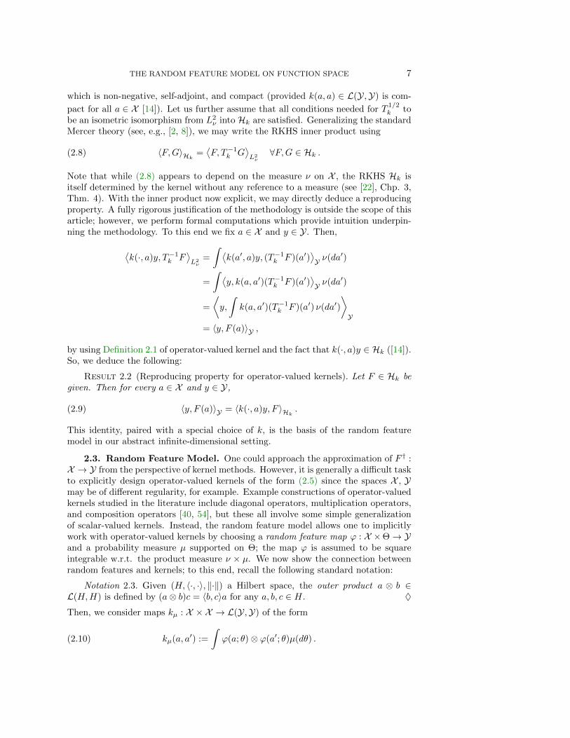
Note that while (2.8) appears to depend on the measure ν on X , the RKHS Hk isitself determined by the kernel without any reference to a measure (see [22], Chp. 3,Thm. 4). With the inner product now explicit, we may directly deduce a reproducingproperty. A fully rigorous justification of the methodology is outside the scope of thisarticle; however, we perform formal computations which provide intuition underpin-ning the methodology. To this end we fix a ∈ X and y ∈ Y. Then,

⟨k(·, a)y, T−1

k F⟩L2ν

=

∫ ⟨k(a′, a)y, (T−1

k F )(a′)⟩Y ν(da′)

=

∫ ⟨y, k(a, a′)(T−1

k F )(a′)⟩Y ν(da′)

=

⟨y,

∫k(a, a′)(T−1

k F )(a′) ν(da′)

⟩Y

= 〈y, F (a)〉Y ,

by using Definition 2.1 of operator-valued kernel and the fact that k(·, a)y ∈ Hk ([14]).So, we deduce the following:

Result 2.2 (Reproducing property for operator-valued kernels). Let F ∈ Hk begiven. Then for every a ∈ X and y ∈ Y,

(2.9) 〈y, F (a)〉Y = 〈k(·, a)y, F 〉Hk .

This identity, paired with a special choice of k, is the basis of the random featuremodel in our abstract infinite-dimensional setting.

2.3. Random Feature Model. One could approach the approximation of F † :X → Y from the perspective of kernel methods. However, it is generally a difficult taskto explicitly design operator-valued kernels of the form (2.5) since the spaces X , Ymay be of different regularity, for example. Example constructions of operator-valuedkernels studied in the literature include diagonal operators, multiplication operators,and composition operators [40, 54], but these all involve some simple generalizationof scalar-valued kernels. Instead, the random feature model allows one to implicitlywork with operator-valued kernels by choosing a random feature map ϕ : X ×Θ→ Yand a probability measure µ supported on Θ; the map ϕ is assumed to be squareintegrable w.r.t. the product measure ν × µ. We now show the connection betweenrandom features and kernels; to this end, recall the following standard notation:

Notation 2.3. Given (H, 〈·, ·〉, ‖·‖) a Hilbert space, the outer product a ⊗ b ∈L(H,H) is defined by (a⊗ b)c = 〈b, c〉a for any a, b, c ∈ H. ♦

Then, we consider maps kµ : X × X → L(Y,Y) of the form

(2.10) kµ(a, a′) :=

∫ϕ(a; θ)⊗ ϕ(a′; θ)µ(dθ) .


Since kµ may readily be shown to be an operator-valued kernel via Definition 2.1,it defines a unique real RKHS Hkµ ⊂ L2

ν(X ;Y). Our approximation theory will bebased on this space or finite-dimensional approximations thereof.

We now perform a purely formal but instructive calculation, following from appli-cation of the reproducing property (2.9) to operator-valued kernels of the form (2.10).Doing so leads to an integral representation of any F † ∈ Hkµ : for all a ∈ X , y ∈ Y,⟨

y, F †(a)⟩Y =

⟨kµ(·, a)y, F †

⟩Hkµ

=

⟨∫〈ϕ(a; θ), y〉Y ϕ(·; θ)µ(dθ), F †

⟩Hkµ

=

∫〈ϕ(a; θ), y〉Y

⟨ϕ(·; θ), F †

⟩Hkµ

µ(dθ)

=

∫c(θ)〈y, ϕ(a; θ)〉Y µ(dθ)

=

⟨y,

∫c(θ)ϕ(a; θ)µ(dθ)

⟩Y,

where the coefficient function c : Θ→ R is defined by

(2.11) c(θ) :=⟨ϕ(·; θ), F †

⟩Hkµ

.

Since Y is Hilbert, the above holding for all y ∈ Y implies the integral representation

(2.12) F † =

∫c(θ)ϕ(·; θ)µ(dθ) .

The expression for c(θ) needs careful interpretation because ϕ(·; θ) /∈ Hkµ with prob-ability one; indeed, c(θ) is defined only as an L2

µ limit. Nonetheless, the RKHS maybe completely characterized by this integral representation. Define

A : L2µ(Θ;R)→ L2

ν(X ;Y)

c 7→ Ac :=

∫c(θ)ϕ(·; θ)µ(dθ) .

(2.13)

Then we have the following result whose proof, provided in Appendix A, is a straight-forward generalization of the real-valued case given in [2], Sec. 2.2:

Result 2.4. Under the assumption that ϕ ∈ L2ν×µ(X ×Θ;Y), the RKHS defined

by the kernel kµ in (2.10) is precisely

(2.14) Hkµ = im(A) =

{∫c(θ)ϕ(·; θ)µ(dθ) : c ∈ L2

µ(Θ;R)

}.

We stress that the integral representation (2.12) is not unique since A is notinjective in general. A central role in what follows is the approximation of measure µby the empirical measure

(2.15) µ(m) :=1

m

m∑j=1

δθj , θj ∼ µ i. i.d.

Given this, define k(m) := kµ(m) to be the empirical approximation to kµ:

(2.16) k(m)(a, a′) = Eθ∼µ(m)

[ϕ(a; θ)⊗ ϕ(a′; θ)] =1

m

m∑j=1

ϕ(a; θj)⊗ ϕ(a′; θj) .


Then define Hk(m) to be the unique RKHS induced by the kernel k(m). The followingcharacterization of Hk(m) is proved in Appendix A:

Result 2.5. Assume that ϕ ∈ L2ν×µ(X × Θ;Y) and that the random features

{ϕ(·; θj)}mj=1 are linearly independent in L2ν(X ;Y). Then, the RKHS Hk(m) is equal

to the linear span of the {ϕj := ϕ(·; θj)}mj=1.

Applying a simple Monte Carlo sampling approach to Equation (2.12), specifi-cally, replacing the probability measure µ by the empirical measure µ(m), gives theapproximation

(2.17) F † ≈ 1

m

m∑j=1

c(θj)ϕ(·; θj) ;

by virtue of Result 2.5, this approximation is in Hk(m) and achieves the Monte Carlorate O(m−1/2). However, in the setting of interest to us, the Monte Carlo approachdoes not give rise to a practical method for two reasons: evaluation of c(θj) requiresknowledge of both the unknown mapping F † and of the RKHS appearing in theinner product defining c from F †; in our setting the kernel kµ of the RKHS is notassumed to be known – only the random features are assumed to be given. To sidestepthese difficulties, the RFM adopts a data-driven optimization approach to determinea different approximation to F †, also from the space Hk(m) .

We now define the RFM:

Definition 2.6. Given probability space (X , ν), with X a real Banach space,probability space (Θ, µ), with Θ a finite or infinite-dimensional Banach space, realseparable Hilbert space Y, and ϕ ∈ L2

ν×µ(X ×Θ;Y), the random feature model isthe parametric map

Fm : X × Rm → Y

(a;α) 7→ Fm(a;α) :=1

m

m∑j=1

αjϕ(a; θj) , θj ∼ µ i. i.d.(2.18)

We implicitly use the Borel σ-algebra to define the probability spaces in thepreceding definition. The goal of the RFM is to choose parameters α ∈ Rm so asto approximate mappings F † ∈ Hkµ by mappings Fm(·;α) ∈ Hk(m) . The RFMmay be viewed as a spectral method since the randomized basis ϕ(·; θ) in the linearexpansion (2.18) is defined on all of X . Determining the coefficient vector α from dataobviates the difficulties associated with the Monte Carlo approach since the methodonly requires knowledge of sample input-output pairs from F † and knowledge of therandom feature map ϕ.

As written, Equation (2.18) is incredibly simple. It is clear that the choice of ran-dom feature map and measure pair (ϕ, µ) will determine the quality of approximation.In their original paper [57], Rahimi and Recht took a kernel-oriented perspective byfirst choosing a kernel and then finding a random feature map to estimate this kernel.Our perspective is the opposite in that we allow the choice of random feature mapϕ to implicitly define the kernel via the formula (2.10) instead of picking the kernelfirst. This methodology also has implications for numerics: the kernel never explicitlyappears in any computations, which leads to storage savings. It does, however, leaveopen the question of characterizing the RKHS Hkµ of mappings from X to Y thatunderlies the approximation method.


The connection to kernels explains the origins of the RFM in the machine learningliterature. Moreover, the RFM may also be interpreted in the context of neuralnetworks. To see this, consider the setting where X , Y are both equal to the Euclideanspace R and choose ϕ to be a family of hidden neurons ϕNN(a; θ) := σ(θ(1) · a+ θ(2)).A single hidden layer NN would seek to find {(αj , θj)}mj=1 in R× R2 so that

(2.19)1

m

m∑j=1

αjϕNN(a; θj)

matches the given training data {ai, yi}ni=1 ⊂ X ×Y. More generally, and in arbitraryEuclidean spaces, one may allow ϕNN(·; θ) to be any deep NN. However, while theRFM has the same form as (2.19), there is a difference in the training : the θj aredrawn i.i.d. from a probability measure and then fixed, and only the αj are chosento fit the training data. This connection is quite profound: given any deep NN withrandomly initialized parameters θ, studies of the lazy training regime and neuraltangent kernel [29, 39] suggest that adopting a RFM approach and optimizing overonly α is quite natural, as it is observed that in this regime the NN parameters donot stray far from their random initialization during gradient descent whilst the lastlayer of parameters αj adapt considerably.

Once the parameters {θj}mj=1 are chosen at random and fixed, training the RFMonly requires optimizing over α ∈ Rm which, due to linearity of Fm in α, is a simpletask to which we now turn our attention.

2.4. Optimization. One of the most attractive characteristics of the RFM isits training procedure. With the L2-type loss (2.4) as in standard regression settings,optimizing the coefficients of the RFM with respect to the empirical risk (2.3) isa convex optimization problem, requiring only the solution of a finite-dimensionalsystem of linear equations; the convexity also suggests the possibility of appendingconvex constraints (such as linear inequalities), although we do not pursue this here.We emphasize the simplicity of the underlying optimization tasks as they suggestthe possibility of numerical implementation of the RFM into complicated black-boxcomputer codes.

We now proceed to show that a regularized version of the optimization prob-lem (2.3)–(2.4) arises naturally from approximation of a nonparametric regressionproblem defined over the RKHS Hkµ . To this end, recall the supervised learning for-mulation in Subsection 2.1. Given n i. i.d. input-output pairs {ai, yi = F †(ai)}ni=1 ⊂X × Y as data, with the ai drawn from unknown probability measure ν on X , theobjective is to find an approximation F ∗ to the map F †. Let Hkµ be the hypothesisspace and kµ its operator-valued reproducing kernel of the form (2.10). The moststraightforward learning algorithm in this RKHS setting is kernel ridge regression,also known as penalized least squares. This method produces a nonparametric modelby finding a minimizer F ∗ of

(2.20) minF∈Hkµ

n∑j=1

1

2‖yj − F (aj)‖2Y +

λ

2‖F‖2Hkµ ,

where λ ≥ 0 is a penalty parameter. By the representer theorem for operator-valuedkernels [54], the minimizer has the form

(2.21) F ∗ =

n∑`=1

kµ(·, a`)β`


for some functions {βj}nj=1 ⊂ Y. In practice, finding these n functions in the outputspace requires solving a (block) linear operator equation. For the high-dimensionalPDE problems we consider in this work, solving such an equation may become prohib-itively expensive from both operation count and storage required. A few workaroundswere proposed in [40] such as certain diagonalizations, but these rely on simplifyingassumptions that are quite limiting. More fundamentally, the representation of thesolution in (2.21) requires knowledge of the kernel kµ; in our setting we assume accessonly to the random features which define kµ and not kµ itself.

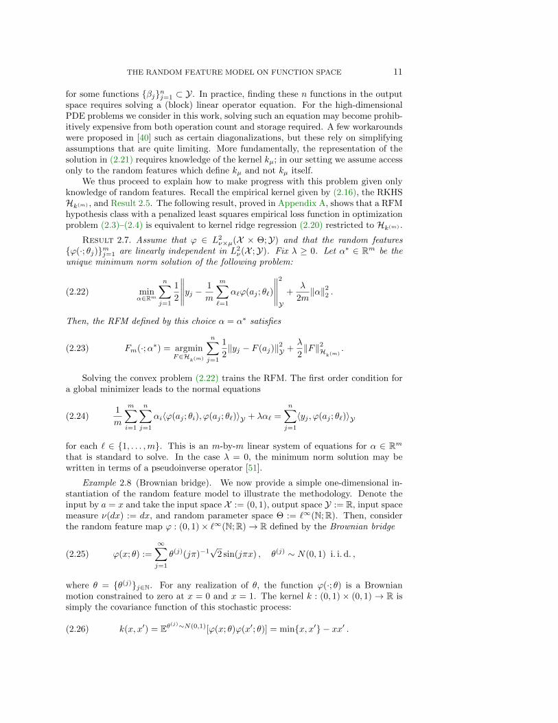
We thus proceed to explain how to make progress with this problem given onlyknowledge of random features. Recall the empirical kernel given by (2.16), the RKHSHk(m) , and Result 2.5. The following result, proved in Appendix A, shows that a RFMhypothesis class with a penalized least squares empirical loss function in optimizationproblem (2.3)–(2.4) is equivalent to kernel ridge regression (2.20) restricted to Hk(m) .

Result 2.7. Assume that ϕ ∈ L2ν×µ(X × Θ;Y) and that the random features

{ϕ(·; θj)}mj=1 are linearly independent in L2ν(X ;Y). Fix λ ≥ 0. Let α∗ ∈ Rm be the

unique minimum norm solution of the following problem:

(2.22) minα∈Rm

n∑j=1

1

2

∥∥∥∥∥yj − 1

m

m∑`=1

α`ϕ(aj ; θ`)

∥∥∥∥∥2

Y

+λ

2m‖α‖22 .

Then, the RFM defined by this choice α = α∗ satisfies

(2.23) Fm(·;α∗) = argminF∈H

k(m)

n∑j=1

1

2‖yj − F (aj)‖2Y +

λ

2‖F‖2H

k(m).

Solving the convex problem (2.22) trains the RFM. The first order condition fora global minimizer leads to the normal equations

(2.24)1

m

m∑i=1

n∑j=1

αi〈ϕ(aj ; θi), ϕ(aj ; θ`)〉Y + λα` =

n∑j=1

〈yj , ϕ(aj ; θ`)〉Y

for each ` ∈ {1, . . . ,m}. This is an m-by-m linear system of equations for α ∈ Rmthat is standard to solve. In the case λ = 0, the minimum norm solution may bewritten in terms of a pseudoinverse operator [51].

Example 2.8 (Brownian bridge). We now provide a simple one-dimensional in-stantiation of the random feature model to illustrate the methodology. Denote theinput by a = x and take the input space X := (0, 1), output space Y := R, input spacemeasure ν(dx) := dx, and random parameter space Θ := `∞(N;R). Then, considerthe random feature map ϕ : (0, 1)× `∞(N;R)→ R defined by the Brownian bridge

(2.25) ϕ(x; θ) :=

∞∑j=1

θ(j)(jπ)−1√

2 sin(jπx) , θ(j) ∼ N(0, 1) i. i.d. ,

where θ = {θ(j)}j∈N. For any realization of θ, the function ϕ(·; θ) is a Brownianmotion constrained to zero at x = 0 and x = 1. The kernel k : (0, 1) × (0, 1) → R issimply the covariance function of this stochastic process:

(2.26) k(x, x′) = Eθ(j)∼N(0,1)[ϕ(x; θ)ϕ(x′; θ)] = min{x, x′} − xx′ .


Note that k is the Green’s function for the negative Laplacian on (0, 1) with Dirichletboundary conditions. Using this fact, we may explicitly characterize the associatedRKHS Hk as follows. First, define

(2.27) Tkf :=

∫ 1

0

k(·, y)f(y) dy =

(− d2

dx2

)−1

f ,

where the the negative Laplacian has domain H10 ((0, 1);R)∩H2((0, 1);R). Viewing Tk

as an operator from L2((0, 1);R) into itself, from (2.8) we conclude, upon integrationby parts,

(2.28) 〈f, g〉Hk =⟨f, T−1

k g⟩L2 =

⟨df

dx,dg

dx

⟩L2

= 〈f, g〉H10∀f, g ∈ Hk ;

note that the last identity does indeed define an inner product on H10 . By this formal

argument we identify the RKHS Hk as the Sobolev space H10 ((0, 1);R). Furthermore,

Brownian bridge may be viewed as the Gaussian measure N(0, Tk). Approximationusing the RFM with the Brownian bridge random feature map is illustrated in Fig-ure 1. Since k(·, x) is a piecewise linear function, a kernel regression method willproduce a piecewise linear approximation. Indeed, the figure indicates that the RFMwith n training points fixed approaches the optimal piecewise linear approximationas m→∞ (see [53] for a related theoretical result). ♦

The Brownian bridge example illuminates a more fundamental idea. For thislow-dimensional problem, an expansion in a deterministic Fourier sine basis would ofcourse be natural. But if we do not have a natural, computable orthonormal basis,then randomness provides a useful alternative representation; notice that the randomfeatures each include random combinations of the deterministic Fourier sine basis inthis Brownian bridge example. For the more complex problems that we move on tostudy numerically in the next two sections, we lack knowledge of good, computablebases for general maps in infinite dimensions. The RFM approach exploits randomnessto allow us to explore, implicitly discover the structure of, and represent, such maps.Thus we now turn away from this example of real-valued maps defined on a subsetof the real line and instead consider the use of random features to represent mapsbetween spaces of functions.

3. Application to PDE Solution Maps. In this section, we design the ran-dom feature maps ϕ : X ×Θ→ Y for the RFM approximation of two particular PDEparameter-to-solution maps: the evolution semigroup of viscous Burgers’ equation inSubsection 3.1 and the coefficient-to-solution operator for the Darcy problem in Sub-section 3.2. As practitioners of kernel methods in machine learning have found, thechoice of kernel (which in this work, follows from the choice of random feature map)plays a central role in the quality of the function reconstruction. While our method ispurely data-driven and requires no knowledge of the governing PDE, we take the viewthat any prior knowledge can, and should, be introduced into the design of ϕ. Themaps ϕ that we employ are nonlinear in both arguments. We also detail the proba-bility measure ν placed on the input space X for each of the two PDE applications;this choice is crucial because while it is desirable that the trained RFM generalizesto arbitrary inputs in X , we can in general only expect to learn an approximation ofthe truth map F † restricted to inputs that resemble those drawn from ν.

3.1. Burgers’ Equation: Formulation. Viscous Burgers’ equation in one spa-tial dimension is representative of the advection-dominated PDE problem class; these


0.0 0.2 0.4 0.6 0.8 1.0x

−0.5

0.0

0.5

1.0

1.5

2.0

2.5

3.0 Test

Truth

Train

(a) m = 50

0.0 0.2 0.4 0.6 0.8 1.0x

−0.5

0.0

0.5

1.0

1.5

2.0

2.5

3.0 Test

Truth

Train

(b) m = 500

0.0 0.2 0.4 0.6 0.8 1.0x

−0.5

0.0

0.5

1.0

1.5

2.0

2.5

3.0 Test

Truth

Train

(c) m = 5000

0.0 0.2 0.4 0.6 0.8 1.0x

−0.5

0.0

0.5

1.0

1.5

2.0

2.5

3.0 Test

Truth

Train

(d) m =∞

Fig. 1: Brownian bridge random feature model for one-dimensional input-output spa-ces with n = 32 training points fixed and λ = 0 (Example 2.8): as m → ∞, theRFM approaches the nonparametric regression solution given by the representer the-orem (Figure 1d), which in this case is a piecewise linear approximation of the truefunction (an element of RKHS Hk = H1

0 , shown in red). Blue lines denote the trainedmodel evaluated on test data points and black circles denote training data points.

time-dependent equations are not conservation laws due to the presence of a smalldissipative term, but nonlinear transport still plays a central role in the evolution ofsolutions. The initial value problem we consider is

(3.1)

∂u

∂t+

∂

∂x

(u2

2

)− ε∂

2u

∂x2= f in (0,∞)× (0, 1)

u(·, 0) = u(·, 1) ,∂u

∂x(·, 0) =

∂u

∂x(·, 1) in (0,∞)

u(0, ·) = a in (0, 1) ,

where ε > 0 is the viscosity (i.e., diffusion coefficient) and we have imposed peri-odic boundary conditions. The initial condition a serves as the input and is drawnaccording to a Gaussian measure defined by

(3.2) a ∼ ν := N(0, C) ,


with covariance operator

(3.3) C = τ2α−d(−∆ + τ2 Id)−α ,

where d = 1 and the operator −∆ is defined on T1. The hyperparameter τ ∈ R+ is aninverse length scale and α > 1/2 controls the regularity of the draw. It is known thatsuch a are Holder with exponent up to α−1/2, so in particular a ∈ X := L2((0, 1);R).Then for all ε > 0, the unique global solution u(t, ·) to (3.1) is real analytic for allt > 0 (see [44], Thm. 1.1). Hence, setting the output space to be Y := Hs((0, 1);R)for any s > 0, we may define the solution map

F † : L2 → Hs

a 7→ F †(a) := ΨT (a) = u(T, ·) ,(3.4)

where {Ψt}t>0 forms the solution operator semigroup for (3.1) and we fix the finaltime t = T > 0. The map F † is smoothing and nonlinear.

We now describe a random feature map for use in the RFM (2.18) that we callFourier space random features. Let F denote the Fourier transform and define ϕ :X ×Θ→ Y by

(3.5) ϕ(a; θ) = σ(F−1(gFθFa)) ,

where σ(·), the ELU function defined below, is defined as a mapping on R and appliedpointwise to vectors. The randomness enters through θ ∼ µ := N(0, C ′), with C ′ thesame covariance operator as in (3.3) but with potentially different inverse length scaleand regularity, and the wavenumber filter function g : R→ R+ is

(3.6) g(k) = σg(δ|k|) , σg(r) := max{0,min{2r, (r + 1/2)−β}} ,

where δ, β > 0. The map ϕ(·; θ) essentially performs a random convolution withthe initial condition followed by a filtering operation. Figure 2a illustrates a sam-ple input and output from ϕ. While not optimized for performance, the filter gis designed to shuffle the energy in low to medium wavenumbers and cut off highwavenumbers (see Figure 2b), reflecting our prior knowledge of the behavior of solu-tions to (3.1).

We choose the activation function σ in (3.5) to be the exponential linear unitELU : R→ R defined by

(3.7) ELU(r) :=

{r , r ≥ 0

er − 1 , r < 0 .

ELU has successfully been used as activation in other machine learning frameworksfor related nonlinear PDE problems [46, 55]. We also find ELU to perform better inthe RFM framework over several other choices including ReLU(·), tanh(·), sigmoid(·),sin(·), SELU(·), and softplus(·). Note that the pointwise evaluation of ELU in (3.5)will be well defined, by Sobolev embedding, for s > 1/2 sufficiently large in thedefinition of Y = Hs. Since the solution operator maps into Hs for any s > 0, thisdoes not constrain the method.


0.0 0.2 0.4 0.6 0.8 1.0x

−0.5

0.0

0.5

1.0

1.5 a

ϕ(a; θ)

(a) (b)

Fig. 2: Random feature map construction for Burgers’ equation: Figure 2a displays arepresentative input-output pair for the random feature ϕ(·; θ) (Equation (3.5)) whileFigure 2b shows the filter function g(k) for δ = 0.0025 and β = 4 (Equation (3.6)).

3.2. Darcy Flow: Formulation. Divergence form elliptic equations [32] arisein a variety of applications, in particular, the groundwater flow in a porous mediumgoverned by Darcy’s law [5]. This linear elliptic boundary value problem reads

(3.8)

{−∇ · (a∇u) = f in D

u = 0 on ∂D ,

where D is a bounded open subset in Rd, f represents sources and sinks of fluid, a thepermeability of the porous medium, and u the piezometric head; all three functionsmap D into R and, in addition, a is strictly positive almost everywhere in D. We workin a setting where f is fixed and consider the input-output map defined by a 7→ u.The measure ν on a is a high contrast level set prior constructed as a pushforward ofa Gaussian measure:

(3.9) a ∼ ν := ψ]N(0, C) ;

here ψ : R→ R is a threshold function defined by

(3.10) ψ(r) = a+1(0,∞)(r) + a−1(−∞,0)(r) , 0 < a− ≤ a+ <∞

and the covariance operator C is given in (3.3) with d = 2 and homogeneous Neu-mann boundary conditions on the Laplacian −∆. That is, the resulting coefficient aalmost surely takes only two values (a+ or a−) and, as the zero level set of a Gaussianrandom field, exhibits random geometry in the physical domain D. It follows thata ∈ L∞(D;R+) almost surely. Further, the size of the contrast ratio a+/a− mea-sures the scale separation of this elliptic problem and hence controls the difficulty ofreconstruction [9]. See Figure 3a for a representative draw.

Given f ∈ L2(D;R), the standard Lax-Milgram theory may be applied to showthat for coefficient a ∈ X := L∞(D;R+), there exists a unique weak solution u ∈


Y := H10 (D;R) for Equation (3.8) (see, e.g., Evans [26]). Thus, we define the ground

truth solution map

F † : L∞ → H10

a 7→ F †(a) := u .(3.11)

We emphasize that while the PDE (3.8) is linear, the solution map F † is nonlinear.We now describe the chosen random feature map for this problem, which we call

predictor-corrector random features. Define ϕ : X ×Θ→ Y by ϕ(a; θ) := p1 such that

−∆p0 =f

a+ σγ(θ1)(3.12a)

−∆p1 =f

a+ σγ(θ2) +∇(log a) · ∇p0 ,(3.12b)

where the boundary conditions are homogeneous Dirichlet, θ = (θ1, θ2) are two Gauss-ian random fields each drawn from measure N(0, C ′), f is the source term in (3.8),and γ = (s+, s−, δ) are parameters for a thresholded sigmoid σγ : R→ R defined by

(3.13) σγ(r) :=s+ − s−

1 + e−r/δ+ s−

and extended as a Nemytskii operator when applied to θ1(·) and θ2(·). In practice,since ∇a is not well-defined when drawn from the level set measure, we replace a withaε, where aε := v(1) is a smoothed version of a obtained by evolving the followinglinear heat equation

(3.14)

dv

dt= η∆v in (0, 1)×D

n · ∇v = 0 on (0, 1)× ∂Dv(0) = a in D

for one time unit. An example of the response of ϕ(·; θ) to a piecewise constant inputa ∼ ν is shown in Figure 3.

We remark that by removing the two random terms involving θ1, θ2 in (3.12), weobtain a remarkably accurate surrogate model for the PDE. This observation is repre-sentative of a more general iterative method, a predictor-corrector type iteration, forsolving the Darcy equation (3.8), which is convergent for sufficiently large coefficientsa. The map ϕ is essentially a random perturbation of a single step of this iterativemethod: Equation (3.12a) makes a coarse prediction of the output, then (3.12b) im-proves this prediction with a correction term (here, this correction term is derivedfrom expanding the original PDE). This choice of ϕ falls within an ensemble view-point that the RFM may be used to improve pre-existing surrogate models by takingϕ(·; θ) to be an existing emulator, but randomized in a principled way through θ.

We are cognizant of the fact that, for this particular example, the random featuremap ϕ requires full knowledge of the Darcy equation and a naıve evaluation of ϕ maybe as expensive as solving the original PDE, which is itself a linear PDE; however,we believe that the ideas underlying the random features used here are intuitive andsuggestive of what is possible in other applications areas. For example, random featuremodels may be applied on domains with simple geometries, which are supersets ofthe physical domain of interest, enabling the use of fast tools such as the fast Fourier


(a) a ∼ ν (b) ϕ(a; θ) , θ ∼ µ

Fig. 3: Random feature map construction for Darcy flow: Figure 3a displays a rep-resentative input draw a with τ = 3, α = 2 and a+ = 12, a− = 3; Figure 3b showsthe output random feature ϕ(a; θ) (Equation (3.12)) taking the coefficient a as input.Here, f ≡ 1, τ ′ = 7.5, α′ = 2, s+ = 1/a+, s− = −1/a−, and δ = 0.15.

transform (FFT) within the RFM even though they may not be available on theoriginal problem, either because the operator to be inverted is spatially inhomogeneousor because of the geometry of the physical domain.

4. Numerical Experiments. We now assess the performance of our proposedmethodology on the approximation of operators F † : X → Y presented in Section 3. Inthe numerical experiments that follow, all infinite-dimensional objects are discretizedon a uniform mesh with K degrees of freedom. In this section, our notation does notmake explicit the dependence on K because the random feature model is consistentwith the continuum in the limit K →∞; we demonstrate this fact numerically.

The input functions and our chosen random feature maps (3.5) and (3.12) requirei. i.d. draws of Gaussian random fields to be fully defined. We efficiently sample thesefields by truncating a Karhunen-Loeve expansion and employing fast summation ofthe eigenfunctions with FFT. More precisely, on a mesh of size K, denote by gθ anumerical representation of a Gaussian random field on domain D = (0, 1)d, d = 1, 2:

(4.1) gθ =∑k∈ZK

ξk√λkφk ≈

∑k′∈(Z+)d

ξk′√λk′φk′ ∼ N(0, C) ,

where ξj ∼ N(0, 1) i. i.d. and ZK ⊂ Z+ is a truncated one-dimensional lattice ofcardinality K ordered such that λj is non-increasing. For clarity, the eigenvalueproblem Cφk = λkφk for non-negative, symmetric, trace-class operator C in (3.3) hassolutions

(4.2) φk(x) = 2 cos(k1πx1) cos(k2πx2) , λk = τ2α−2(π2|k|2 + τ2)−α

for homogeneous Neumann boundary conditions when d = 2, k = (k1, k2) ∈ (Z+)2,x = (x1, x2) ∈ (0, 1)2, and solutions

(4.3) φk(x) = e2πikx , λk = τ2α−1(4π2k2 + τ2)−α


for periodic boundary conditions when d = 1, k ∈ Z, x ∈ (0, 1) (with appropriatelymodified random variables ξj in (4.1) to ensure that the resulting gθ is real-valued).These forms of gθ are used in all experiments that follow.

To measure the distance between the RFM approximation Fm(·;α∗) and theground truth map F †, we employ the approximate expected relative test error

(4.4) en′,m :=1

n′

n′∑j=1

∥∥F †(aj)− Fm(aj ;α∗)∥∥L2

‖F †(aj)‖L2

≈ Ea∼ν∥∥F †(a)− Fm(a;α∗)

∥∥L2

‖F †(a)‖L2

,

where the {aj}n′

j=1 are drawn i.i.d. from ν and n′ denotes the number of input-output

pairs used in testing. All L2(D;R) norms on the physical domain are numericallyapproximated by trapezoid rule quadrature. Since Y ⊂ L2(D;R) for both the PDEsolution operators (3.4) and (3.11), we also perform all required inner products duringtraining in L2(D;R) rather than in Y; this results in smaller relative test error en′,m.

4.1. Burgers’ Equation: Experiment. We generate a high resolution datasetof input-output pairs by solving Burgers’ equation (3.1) on a uniform periodic meshof size K = 1025 (identifying the first mesh point with the last) using an FFT-based pseudospectral method for spatial discretization and a fourth-order Runge-Kutta integrating factor time-stepping scheme [41] for time discretization. All meshsizes K < 1025 are subsampled from this original dataset and hence we considernumerical realizations of F † up to R1025 → R1025. We fix n = 512 training andn′ = 4000 testing pairs unless otherwise noted. The input data are drawn fromν = N(0, C) where C is given by (3.3) with parameter choices τ = 7 and α = 2.5. Wefix the viscosity to ε = 10−2 in all experiments. Lowering ε leads to smaller lengthscale solutions and more difficult reconstruction; more data (higher n) and features(higher m) or a more expressive choice of ϕ would be required to achieve comparableerror levels. For simplicity, we set the forcing f ≡ 0, although nonzero forcing couldlead to other interesting solution maps such as f 7→ u(T, ·). It is easy to check that thesolution will have zero mean for all time and a steady state of zero. Hence, we chooseT ≤ 2 to ensure that the solution is far from attaining steady state. For the randomfeature map (3.5), we fix the hyperparameters α′ = 2, τ ′ = 5, δ = 0.0025, and β = 4.The map itself is evaluated efficiently with the FFT, and hyperparameters were notoptimized. We find that regularization during training has a negligible effect for ourproblem, so the RFM is trained with λ = 0 by solving the normal equations (2.24)with the pseudoinverse to deliver the minimum norm least squares solution; we usethe truncated SVD implementation in scipy.linalg.pinv2 for this purpose.

Our experiments study the RFM approximation to the viscous Burgers’ equationevolution operator semigroup (3.4). As a visual aid for the high-dimensional problemat hand, Figure 4 shows a representative sample input and output along with a trainedRFM test prediction. To determine whether the RFM has actually learned the correctevolution operator, we test the semigroup property of the map. Denote the (j−1)-foldcomposition of a function F with itself by F j . Then, with u(0, ·) = a, we have

(4.5) (ΨT ◦ · · · ◦ΨT )(a) = ΨjT (a) = ΨjT (a) = u(rT, ·)

by definition. We train the RFM on input-output pairs from the map ΨT with T := 0.5to obtain F∗ := Fm(·;α∗). Then, it should follow from (4.5) that F j∗ ≈ ΨjT , that is,each application of F∗ should evolve the solution T time units. We test this semigroupapproximation by learning the map F∗ and then comparing F j∗ on n′ = 4000 fixed


0.0 0.2 0.4 0.6 0.8 1.0x

−0.4

−0.2

0.0

0.2

0.4

Input

Test

Truth

(a) (b)

Fig. 4: Representative input-output test sample for the Burgers’ equation solutionmap F † := Ψ1: Here, n = 512, m = 1024, and K = 1025. Figure 4a shows a sampleinput, output (truth), and trained RFM prediction (test), while Figure 4b displaysthe pointwise error. The relative L2 error for this single prediction is 0.0146.

inputs to outputs from each of the operators ΨjT , with j ∈ {1, 2, 3, 4} (the solutionsat time T , 2T , 3T , 4T ). The results are presented in Table 1 for a fixed mesh sizeK = 129. We observe that the composed RFM map F j∗ accurately captures ΨjT ,

Train on: T = 0.5 Test on: 2T = 1.0 3T = 1.5 4T = 2.0

0.0360 0.0407 0.0528 0.0788

Table 1: Expected relative error en′,m for time upscaling with the learned RFMoperator semigroup for Burgers’ equation: Here, n′ = 4000, m = 1024, n = 512,and K = 129. The RFM is trained on data from the evolution operator ΨT=0.5,and then tested on input-output samples generated from ΨjT , where j = 2, 3, 4, byrepeated composition of the learned model. The error increase is small even after threecompositions of the learned RFM map, reflecting excellent generalization ability.

though this accuracy deteriorates as j increases due to error propagation. However,even after three compositions corresponding to 1.5 time units past the training timeT = 0.5, the relative error only increases by around 0.04. It is remarkable thatthe RFM learns time evolution without explicitly time-stepping the PDE (3.1) itself.Such a procedure is coined time upscaling in the PDE context and in some sensebreaks the CFL stability barrier [23]. Table 1 is evidence that the RFM has excellentgeneralization properties: while only trained on inputs a ∼ ν, the model predicts wellon new input samples ΨjT (a) ∼ (ΨjT )]ν.

We next study the ability of the RFM to transfer its learned coefficients α∗ ob-tained from training on mesh size K to different mesh resolutions K ′ in Figure 5a. Wefix T := 1 from here on and observe that the lowest test error occurs when K = K ′,


that is, when the train and test resolutions are identical; this behavior was also ob-served in the contemporaneous work [48]. Still, the errors are essentially constantacross resolution, indicating that the RFM learns its optimal coefficients indepen-dently of the resolution and hence generalizes well to any desired mesh size. In fact,the trained model could employ different discretization methodologies (e.g.: finiteelement, spectral) for its random feature map, not just different mesh sizes.

0 200 400 600 800 1000Resolution

0.030

0.035

0.040

0.045

0.050

0.055

0.060

Exp

ecte

dR

elat

ive

Tes

tE

rror

Train on K = 65

Train on K = 257

Train on K = 1025

(a)

0 200 400 600 800 1000m

0.05

0.10

0.15

0.20

0.25

Exp

ecte

dR

elat

ive

Tes

tE

rror

n = 10

n = 20

n = 30

n = 100

n = 1000

(b)

Fig. 5: Expected relative test error of a trained RFM for the Burgers’ equation evo-lution operator F † = Ψ1 with n′ = 4000 test pairs: Figure 5a displays the invarianceof test error w.r.t. training and testing on different resolutions for m = 1024 andn = 512 fixed; the RFM can train and test on different mesh sizes without loss ofaccuracy. Figure 5b shows the decay of the test error for resolution K = 129 fixedas a function of m and n; the smallest error achieved is 0.0303 for n = 1000 andm = 1024.

The smallest expected relative test error achieved by the RFM is 0.0303 for theconfiguration detailed in Figure 5b. In this figure, we also note that for a smallnumber of training data n, the error does not always decrease as the number of randomfeatures m increases. This indicates a delicate dependence of m as a function of n,in particular, n must increase with m; we observe the desired monotonic decrease inerror with m when n is increased to 100 or 1000. In the over-parametrized regime, theauthors in [53] presented a loose bound for this dependence for real-valued outputs.We leave a detailed account of the dependence of m on n required to achieve a certainerror tolerance to future work.

Finally, Figure 6 demonstrates the invariance of the expected relative test errorto the mesh resolution used for training and testing. This result is a consequenceof framing the RFM on function space; other methods defined in finite-dimensionsexhibit an increase in test error as mesh resolution is increased (see [11], Sec. 4,for a numerical account of this phenomenon). The first panel, Figure 6a, shows theerror as a function of mesh resolution for three values of m. For very low resolution,the error varies slightly but then flattens out to a constant value as K → ∞. Moreinterestingly, these constant values of error, en′,m = 0.063, 0.043, and 0.031 corre-sponding to m = 256, 512, and 1024, respectively, closely match the Monte Carlo rate


0 200 400 600 800 1000Resolution

0.030

0.035

0.040

0.045

0.050

0.055

0.060

Exp

ecte

dR

elat

ive

Tes

tE

rror m = 256

m = 512

m = 1024

(a)

0 100 200 300 400 500Resolution

10−3

10−2

10−1

‖α(K

)−α

(1025)‖ 2/‖α

(1025)‖ 2

m = 256

m = 512

m = 1024

(b)

Fig. 6: Results of a trained RFM for the Burgers’ equation evolution operatorF † = Ψ1: Here, n = 512 training and n′ = 4000 testing pairs were used. Fig-ure 6a demonstrates resolution-invariant test error for various m; the error followsthe O(m−1/2) Monte Carlo rate remarkably well. Figure 6b displays the relative errorof the learned coefficient α w.r.t. the coefficient learned on the highest mesh size(K = 1025).

O(m−1/2). While more theory is required to understand this behavior, it indicatesthat the optimization process is finding coefficients close to those arising from a MonteCarlo approximation of the ground truth map F † as discussed in Subsection 2.3. Thesecond panel, Figure 6b, indicates that the learned coefficient α(K) for each K con-verges to some α(∞) as K →∞, again reflecting the design of the RFM as a mappingbetween infinite-dimensional spaces.

4.2. Darcy Flow: Experiment. In this section, we consider Darcy flow on thephysical domain D := (0, 1)2, the unit square. We generate a high resolution datasetof input-output pairs by solving Equation (3.8) on a uniform 257 × 257 mesh (sizeK = 2572) using a second order finite difference scheme. All mesh sizes K < 2572 aresubsampled from this original dataset and hence we consider numerical realizationsof F † up to R66049 → R66049. We denote resolution by r such that K = r2. Wefix n = 128 training and n′ = 1000 testing pairs unless otherwise noted. The inputdata are drawn from the level set measure ν (3.9) with τ = 3 and α = 2 fixed. Wechoose a+ = 12 and a− = 3 in all experiments that follow and hence the contrast ratioa+/a− = 4 is fixed. The source is fixed to f ≡ 1, the constant function. We evaluatethe predictor-corrector random features ϕ (3.12) using an FFT-based fast Poissonsolver corresponding to an underlying second order finite difference stencil at a costof O(K logK) per solve. The smoothed coefficient aε in the definition of ϕ is obtainedby solving (3.14) with time step 0.03 and diffusion constant η = 10−4; with centeredsecond order finite differences, this incurs 34 time steps and hence a cost O(34K).We fix the hyperparameters α′ = 2, τ ′ = 7.5, s+ = 1/12, s− = −1/3, and δ = 0.15for the map ϕ. Unlike in Subsection 4.1, we find that regularization during trainingdoes improve the reconstruction of the Darcy flow solution operator and hence wetrain with λ := 10−8 fixed. We remark that none of these hyperparameters were


optimized, so the RFM performance has the capacity to improve beyond the resultswe demonstrate in this section.

(a) Truth (b) Approximation

(c) Input (d) Pointwise Error

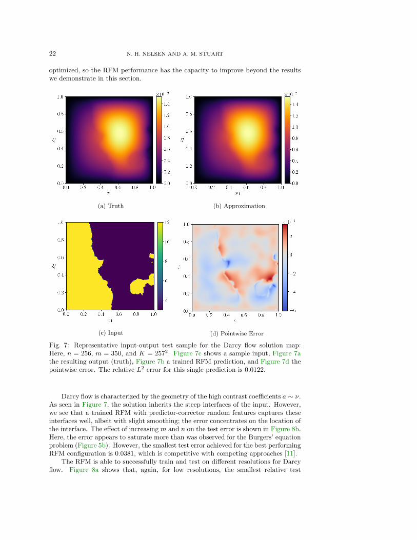
Fig. 7: Representative input-output test sample for the Darcy flow solution map:Here, n = 256, m = 350, and K = 2572. Figure 7c shows a sample input, Figure 7athe resulting output (truth), Figure 7b a trained RFM prediction, and Figure 7d thepointwise error. The relative L2 error for this single prediction is 0.0122.

Darcy flow is characterized by the geometry of the high contrast coefficients a ∼ ν.As seen in Figure 7, the solution inherits the steep interfaces of the input. However,we see that a trained RFM with predictor-corrector random features captures theseinterfaces well, albeit with slight smoothing; the error concentrates on the location ofthe interface. The effect of increasing m and n on the test error is shown in Figure 8b.Here, the error appears to saturate more than was observed for the Burgers’ equationproblem (Figure 5b). However, the smallest test error achieved for the best performingRFM configuration is 0.0381, which is competitive with competing approaches [11].

The RFM is able to successfully train and test on different resolutions for Darcyflow. Figure 8a shows that, again, for low resolutions, the smallest relative test


error is achieved when the train and test resolutions are identical (here, for r = 17);however, when the resolution is increased, the relative test error slightly increasesthen approaches a constant value, reflecting the function space design of the method.Training the RFM on a high resolution mesh poses no issues when transferring tolower resolution meshes for model evaluation, and it achieves consistent error for testresolutions sufficiently large (r ≥ 33).

0 50 100 150 200 250Resolution

0.04

0.06

0.08

0.10

0.12

Exp

ecte

dR

elat

ive

Tes

tE

rror

Train on r = 17

Train on r = 129

(a)

0 100 200 300 400 500m

10−1E

xp

ecte

dR

elat

ive

Tes

tE

rror

n = 5

n = 10

n = 20

n = 50

n = 500

(b)

Fig. 8: Expected relative test error of a trained RFM for Darcy flow with n′ = 1000test pairs: Figure 8a displays the invariance of test error w.r.t. training and testingon different resolutions for m = 512 and n = 256 fixed; the RFM can train and teston different mesh sizes without significant loss of accuracy. Figure 8b shows the decayof the test error for resolution r = 33 fixed as a function of m and n; the smallesterror achieved is 0.0381 for n = 500 and m = 512.

In Figure 9, we again confirm that our method is invariant to the refinement of themesh and improves with more random features. While the difference at low resolutionsis more pronounced than that observed for Burgers’ equation, our results for Darcyflow still suggest that the expected relative test error approaches a constant valueas resolution increases; an estimate of this rate of convergence is seen in Figure 9b,where we plot the relative error of the learned parameter α(r) at resolution r w.r.t.the parameter learned at the highest resolution trained, which was r = 129. Althoughwe do not observe the limiting error following the Monte Carlo rate, which suggeststhat perhaps the RKHS Hkµ induced by the choice of ϕ is not expressive enough,the numerical results make clear that our methodology nonetheless performs well asa function approximator.

5. Conclusions. In this article, we introduced a random feature methodologyfor pure data-driven approximation of mappings F † : X → Y between infinite-dimensional Banach spaces. The random feature model Fm(·;α∗), as an emulatorof such maps, performs dimension reduction in the sense that the original problem offinding F † is reduced to an approximate problem of finding m real numbers α∗ ∈ Rm(Section 2). While it does not immediately follow that the learned model Fm(·;α∗) isnecessarily cheaper to evaluate than a full order solver for F †, our design of problem-


0 25 50 75 100 125Resolution

0.040

0.045

0.050

0.055

0.060

0.065

0.070

Exp

ecte

dR

elat

ive

Tes

tE

rror

m = 64

m = 128

m = 256

(a)

0 20 40 60Resolution

10−2

10−1

100

‖α(r

)−α

(129

) ‖2/‖α

(129) ‖

2

m = 64

m = 128

m = 256

(b)

Fig. 9: Results of a trained RFM for Darcy flow: Here, n = 128 training and n′ = 1000testing pairs were used. Figure 9a demonstrates resolution-invariant test error forvarious m, while Figure 9b displays the relative error of the learned coefficient α(r)

at resolution r w.r.t. the coefficient learned on the highest resolution (r = 129).

specific random feature maps in Section 3 leads to efficient O(mK logK) evaluation ofthe RFM for simple physical domain geometries and hence competitive computationalcost in many-query settings.

Our non-intrusive methodology for high-dimensional approximation is one of onlya select few [11, 48] that first designs a model in infinite dimensions, then discretizes;most other works in this line of research discretize the problem first, and then designa model between finite-dimensional spaces. Our conceptually infinite-dimensional al-gorithm results in a method that is consistent with the continuum picture, robustto discretization, and leads to more flexibility during practical use. For example,discretization of the input-output Banach spaces X , Y is required for practical im-plementation and leads to high-dimensional functions RK → RK . But as a methodconceptualized on function space, the RFM is defined without any reference to a dis-cretization and thus its approximation quality is consistent across different choicesof mesh size K; indeed, the RFM could be trained on one method, say a spectraldiscretization, and deployed using another, say finite element or finite difference dis-cretization. Furthermore, the RFM basis functions, that is, the random feature mapsϕ, are defined independently of the training data unlike in competing approachessuch as the reduced basis method or the method in [11]; hence, our model may bedirectly evaluated on any mesh resolution once trained. These benefits were verifiedin numerical experiments for two nonlinear problems based on PDEs, one involving asemigroup and another a coefficient-to-solution operator (Section 4).

We remark that while our FFT implementations of the random feature mapsin Section 3 have time complexity O(K logK), this may be improved to the optimallinear O(K) with fast multipole or multigrid methods [31]. Although the methodis implemented on uniform grids in space for speed and simplicity, the theoreticalformulation we introduced for the RFM on function space holds irrespective of thediscretization and hence an interesting extension of this work would design cheap-to-


evaluate random feature maps on unstructured grids, perhaps making the RFM moreapplicable to real experimental data or in applications outside of PDEs.

There are various other interesting directions for future work based on our ran-dom feature methodology. We are interested in application of the method to morechallenging problems in the sciences such as climate modeling and material model-ing, and to the solution of design and inverse problems arising in those settings, withthe RFM serving as a cheap emulator. Furthermore, we wish to investigate a non-parametric generalization of the RFM inspired by moving least squares (MLS) [72];MLS shares many parallels to the RFM and the reduced basis method that have yetto be explored. Also of interest is the question of allowing θ in ϕ(·; θ) to adapt todata, for example, via sparsity constraints in the training of the RFM or solving anon-convex optimization problem obtained by choosing ϕ to be a neural network (de-signed in infinite dimensions) with trainable hidden parameters. Such explorationswould serve to further clarify the effectiveness of function space learning algorithms.Finally, the development of a theory which underpins our method, and allows forproof of convergence, would be both mathematically challenging and highly desirable.

Acknowledgments. The authors are grateful to Bamdad Hosseini and NikolaB. Kovachki for helpful input which improved this work.

REFERENCES

[1] N. Aronszajn, Theory of reproducing kernels, Transactions of the American MathematicalSociety, 68 (1950), pp. 337–404.

[2] F. Bach, On the equivalence between kernel quadrature rules and random feature expansions,The Journal of Machine Learning Research, 18 (2017), pp. 714–751.

[3] Y. Bar-Sinai, S. Hoyer, J. Hickey, and M. P. Brenner, Learning data-driven discretizationsfor partial differential equations, Proceedings of the National Academy of Sciences, 116(2019), pp. 15344–15349.

[4] M. Barrault, Y. Maday, N. C. Nguyen, and A. T. Patera, An empirical interpolation-method: application to efficient reduced-basis discretization of partial differential equations,Comptes Rendus Mathematique, 339 (2004), pp. 667–672.

[5] J. Bear and M. Y. Corapcioglu, Fundamentals of transport phenomena in porous media,vol. 82, Springer Science & Business Media, 2012.

[6] M. Belkin, D. Hsu, S. Ma, and S. Mandal, Reconciling modern machine-learning practiceand the classical bias–variance trade-off, Proceedings of the National Academy of Sciences,116 (2019), pp. 15849–15854.

[7] P. Benner, A. Cohen, M. Ohlberger, and K. Willcox, Model reduction and approximation:theory and algorithms, vol. 15, SIAM, 2017.

[8] A. Berlinet and C. Thomas-Agnan, Reproducing kernel Hilbert spaces in probability andstatistics, Springer Science & Business Media, 2011.

[9] C. Bernardi and R. Verfurth, Adaptive finite element methods for elliptic equations withnon-smooth coefficients, Numerische Mathematik, 85 (2000), pp. 579–608.

[10] G. Beylkin and M. J. Mohlenkamp, Algorithms for numerical analysis in high dimensions,SIAM Journal on Scientific Computing, 26 (2005), pp. 2133–2159.

[11] K. Bhattacharya, B. Hosseini, N. B. Kovachki, and A. M. Stuart, Model reduction andneural networks for parametric pdes, arXiv preprint arXiv:2005.03180, (2020).

[12] D. Bigoni, Y. Chen, N. G. Trillos, Y. Marzouk, and D. Sanz-Alonso, Data-driven forwarddiscretizations for Bayesian inversion, arXiv preprint arXiv:2003.07991, (2020).

[13] Y. Cao and Q. Gu, Generalization bounds of stochastic gradient descent for wide and deepneural networks, in Advances in Neural Information Processing Systems, 2019, pp. 10835–10845.

[14] C. Carmeli, E. De Vito, and A. Toigo, Vector valued reproducing kernel Hilbert spaces ofintegrable functions and Mercer theorem, Analysis and Applications, 4 (2006), pp. 377–408.

[15] G. Chen and K. Fidkowski, Output-based error estimation and mesh adaptation using con-volutional neural networks: Application to a scalar advection-diffusion problem, in AIAAScitech 2020 Forum, 2020, p. 1143.


[16] T. Chen and H. Chen, Universal approximation to nonlinear operators by neural networks witharbitrary activation functions and its application to dynamical systems, IEEE Transactionson Neural Networks, 6 (1995), pp. 911–917.

[17] M. Cheng, T. Y. Hou, M. Yan, and Z. Zhang, A data-driven stochastic method for ellip-tic PDEs with random coefficients, SIAM/ASA Journal on Uncertainty Quantification, 1(2013), pp. 452–493.

[18] A. Chkifa, A. Cohen, R. DeVore, and C. Schwab, Sparse adaptive taylor approximationalgorithms for parametric and stochastic elliptic pdes, ESAIM: Mathematical Modellingand Numerical Analysis, 47 (2013), pp. 253–280.

[19] A. Cohen and R. DeVore, Approximation of high-dimensional parametric PDEs, Acta Nu-merica, 24 (2015), pp. 1–159.

[20] A. Cohen and G. Migliorati, Optimal weighted least-squares methods, arXiv preprintarXiv:1608.00512, (2016).

[21] S. L. Cotter, G. O. Roberts, A. M. Stuart, and D. White, Mcmc methods for functions:modifying old algorithms to make them faster, Statistical Science, (2013), pp. 424–446.

[22] F. Cucker and S. Smale, On the mathematical foundations of learning, Bulletin of the Amer-ican mathematical society, 39 (2002), pp. 1–49.

[23] L. Demanet, Curvelets, wave atoms, and wave equations, PhD thesis, California Institute ofTechnology, 2006.

[24] R. A. DeVore, The theoretical foundation of reduced basis methods, Model Reduction andapproximation: Theory and Algorithms, (2014), pp. 137–168.

[25] A. Doostan and G. Iaccarino, A least-squares approximation of partial differential equa-tions with high-dimensional random inputs, Journal of Computational Physics, 228 (2009),pp. 4332–4345.

[26] L. C. Evans, Partial differential equations, vol. 19, American Mathematical Soc., 2010.[27] Y. Fan and L. Ying, Solving electrical impedance tomography with deep learning, Journal of

Computational Physics, 404 (2020), pp. 109–119.[28] J. Feliu-Faba, Y. Fan, and L. Ying, Meta-learning pseudo-differential operators with deep

neural networks, Journal of Computational Physics, 408 (2020), p. 109309.[29] H. Gao, J.-X. Wang, and M. J. Zahr, Non-intrusive model reduction of large-scale, nonlinear

dynamical systems using deep learning, arXiv preprint arXiv:1911.03808, (2019).[30] M. Geist, P. Petersen, M. Raslan, R. Schneider, and G. Kutyniok, Numerical so-

lution of the parametric diffusion equation by deep neural networks, arXiv preprintarXiv:2004.12131, (2020).

[31] A. Gholami, D. Malhotra, H. Sundar, and G. Biros, Fft, fmm, or multigrid? a comparativestudy of state-of-the-art poisson solvers for uniform and nonuniform grids in the unit cube,SIAM Journal on Scientific Computing, 38 (2016), pp. C280–C306.

[32] D. Gilbarg and N. S. Trudinger, Elliptic partial differential equations of second order,springer, 2015.

[33] R. Gonzalez-Garcia, R. Rico-Martinez, and I. Kevrekidis, Identification of distributedparameter systems: A neural net based approach, Computers & chemical engineering, 22(1998), pp. S965–S968.

[34] M. Griebel and C. Rieger, Reproducing kernel Hilbert spaces for parametric partial differen-tial equations, SIAM/ASA Journal on Uncertainty Quantification, 5 (2017), pp. 111–137.

[35] E. Haber and L. Ruthotto, Stable architectures for deep neural networks, Inverse Problems,34 (2017), p. 014004.

[36] T. Hastie, R. Tibshirani, and J. Friedman, The elements of statistical learning: data mining,inference, and prediction, Springer Science & Business Media, 2009.

[37] J. S. Hesthaven and S. Ubbiali, Non-intrusive reduced order modeling of nonlinear problemsusing neural networks, Journal of Computational Physics, 363 (2018), pp. 55–78.

[38] M. Hinze, R. Pinnau, M. Ulbrich, and S. Ulbrich, Optimization with PDE constraints,vol. 23, Springer Science & Business Media, 2008.

[39] A. Jacot, F. Gabriel, and C. Hongler, Neural tangent kernel: Convergence and general-ization in neural networks, in Advances in neural information processing systems, 2018,pp. 8571–8580.

[40] H. Kadri, E. Duflos, P. Preux, S. Canu, A. Rakotomamonjy, and J. Audiffren,Operator-valued kernels for learning from functional response data, The Journal of Ma-chine Learning Research, 17 (2016), pp. 613–666.

[41] A.-K. Kassam and L. N. Trefethen, Fourth-order time-stepping for stiff PDEs, SIAM Jour-nal on Scientific Computing, 26 (2005), pp. 1214–1233.

[42] R. Kempf, H. Wendland, and C. Rieger, Kernel-based reconstructions for parametricPDEs, in International Workshop on Meshfree Methods for Partial Differential Equations,


Springer, 2017, pp. 53–71.[43] Y. Khoo, J. Lu, and L. Ying, Solving parametric pde problems with artificial neural networks,

arXiv preprint arXiv:1707.03351, (2017).[44] A. Kiselev, F. Nazarov, and R. Shterenberg, Blow up and regularity for fractal burgers

equation, arXiv preprint arXiv:0804.3549, (2008).[45] G. Kutyniok, P. Petersen, M. Raslan, and R. Schneider, A theoretical analysis of deep

neural networks and parametric PDEs, arXiv preprint arXiv:1904.00377, (2019).[46] K. Lee and K. T. Carlberg, Model reduction of dynamical systems on nonlinear mani-

folds using deep convolutional autoencoders, Journal of Computational Physics, 404 (2020),p. 108973.

[47] Y. Li, J. Lu, and A. Mao, Variational training of neural network approximations of solutionmaps for physical models, Journal of Computational Physics, 409 (2020), p. 109338.

[48] Z. Li, N. Kovachki, K. Azizzadenesheli, B. Liu, K. Bhattacharya, A. Stuart, andA. Anandkumar, Neural operator: Graph kernel network for partial differential equa-tions, arXiv preprint arXiv:2003.03485, (2020).

[49] Z. Long, Y. Lu, X. Ma, and B. Dong, Pde-net: Learning PDEs from data, arXiv preprintarXiv:1710.09668, (2017).

[50] L. Lu, P. Jin, and G. E. Karniadakis, Deeponet: Learning nonlinear operators for identifyingdifferential equations based on the universal approximation theorem of operators, arXivpreprint arXiv:1910.03193, (2019).

[51] D. G. Luenberger, Optimization by vector space methods, John Wiley & Sons, 1997.[52] C. Ma, L. Wu, and E. Weinan, Machine learning from a continuous viewpoint, arXiv preprint

arXiv:1912.12777, (2019).[53] C. Ma, L. Wu, and E. Weinan, On the generalization properties of minimum-norm solutions

for over-parameterized neural network models, arXiv preprint arXiv:1912.06987, (2019).[54] C. A. Micchelli and M. Pontil, On learning vector-valued functions, Neural computation,

17 (2005), pp. 177–204.[55] R. G. Patel and O. Desjardins, Nonlinear integro-differential operator regression with neural

networks, arXiv preprint arXiv:1810.08552, (2018).[56] B. Peherstorfer, K. Willcox, and M. Gunzburger, Survey of multifidelity methods in

uncertainty propagation, inference, and optimization, Siam Review, 60 (2018), pp. 550–591.

[57] A. Rahimi and B. Recht, Random features for large-scale kernel machines, in Advances inneural information processing systems, 2008, pp. 1177–1184.

[58] M. Raissi, P. Perdikaris, and G. E. Karniadakis, Physics-informed neural networks: A deeplearning framework for solving forward and inverse problems involving nonlinear partialdifferential equations, Journal of Computational Physics, 378 (2019), pp. 686–707.

[59] R. Rico-Martinez, K. Krischer, I. Kevrekidis, M. Kube, and J. Hudson, Discrete-vs.continuous-time nonlinear signal processing of cu electrodissolution data, Chemical Engi-neering Communications, 118 (1992), pp. 25–48.

[60] F. Rossi and B. Conan-Guez, Functional multi-layer perceptron: a non-linear tool for func-tional data analysis, Neural networks, 18 (2005), pp. 45–60.

[61] L. Ruthotto and E. Haber, Deep neural networks motivated by partial differential equations,Journal of Mathematical Imaging and Vision, (2019), pp. 1–13.

[62] N. D. Santo, S. Deparis, and L. Pegolotti, Data driven approximation of parametrizedPDEs by reduced basis and neural networks, arXiv preprint arXiv:1904.01514, (2019).

[63] C. Schwab and J. Zech, Deep learning in high dimension: Neural network expression ratesfor generalized polynomial chaos expansions in uq, Analysis and Applications, 17 (2019),pp. 19–55.

[64] J. Sirignano and K. Spiliopoulos, Dgm: A deep learning algorithm for solving partial dif-ferential equations, Journal of Computational Physics, 375 (2018), pp. 1339–1364.

[65] P. D. Spanos and R. Ghanem, Stochastic finite element expansion for random media, Journalof engineering mechanics, 115 (1989), pp. 1035–1053.

[66] Y. Sun, A. Gilbert, and A. Tewari, Random relu features: Universality, approximation, andcomposition, stat, 1050 (2018), p. 10.

[67] N. Trask, R. G. Patel, B. J. Gross, and P. J. Atzberger, Gmls-nets: A framework forlearning from unstructured data, arXiv preprint arXiv:1909.05371, (2019).

[68] R. K. Tripathy and I. Bilionis, Deep uq: Learning deep neural network surrogate models forhigh dimensional uncertainty quantification, Journal of computational physics, 375 (2018),pp. 565–588.

[69] E. Weinan, A proposal on machine learning via dynamical systems, Communications in Math-ematics and Statistics, 5 (2017), pp. 1–11.


[70] E. Weinan, J. Han, and Q. Li, A mean-field optimal control formulation of deep learning,Research in the Mathematical Sciences, 6 (2019), p. 10.

[71] E. Weinan and B. Yu, The deep ritz method: a deep learning-based numerical algorithm forsolving variational problems, Communications in Mathematics and Statistics, 6 (2018),pp. 1–12.

[72] H. Wendland, Scattered data approximation, vol. 17, Cambridge university press, 2004.[73] C. K. Williams, Computing with infinite networks, in Advances in neural information process-

ing systems, 1997, pp. 295–301.[74] C. K. Williams and C. E. Rasmussen, Gaussian processes for machine learning, vol. 2, MIT

press Cambridge, MA, 2006.[75] N. Winovich, K. Ramani, and G. Lin, Convpde-uq: Convolutional neural networks with

quantified uncertainty for heterogeneous elliptic partial differential equations on varieddomains, Journal of Computational Physics, 394 (2019), pp. 263–279.

[76] Y. Zhu and N. Zabaras, Bayesian deep convolutional encoder–decoder networks for surrogatemodeling and uncertainty quantification, Journal of Computational Physics, 366 (2018),pp. 415–447.

Appendix A. Proofs of Results.

Proof of Result 2.4. Fix a ∈ X and y ∈ Y. Then, we note that

(A.1) kµ(·, a)y =

∫〈ϕ(a; θ), y〉Yϕ(·; θ)µ(dθ) = A〈ϕ(a; ·), y〉Y ∈ im(A) ,

since 〈ϕ(a; ·), y〉Y ∈ L2µ(Θ;R) by the Cauchy-Schwarz inequality.

Now, we show that im(A) admits a reproducing property of the form (2.9). First,note that A can be viewed as a bijection between its coimage and image spaces, andwe denote this bijection by A:

(A.2) A : ker(A)⊥ → im(A) .

For any F, G ∈ im(A), define the candidate RKHS inner product 〈·, ·〉 by

(A.3) 〈F,G〉 := 〈A−1F, A−1G〉L2µ(Θ;R) ;

this is indeed a valid inner product since A is invertible. Note that for any q ∈ ker(A),

⟨q, 〈ϕ(a; ·), y〉Y

⟩L2µ(Θ;R)

=

∫q(θ)〈ϕ(a; θ), y〉Y µ(dθ)

=

⟨∫q(θ)ϕ(a; θ)µ(dθ), y

⟩Y

= 0

so that 〈ϕ(a; ·), y〉Y ∈ ker(A)⊥. Then, we compute

〈kµ(·, a)y, F 〉 =⟨〈ϕ(a; ·), y〉Y , A−1F

⟩L2µ(Θ;R)

=

∫〈ϕ(a; θ), y〉Y(A−1F )(θ)µ(dθ)

=

⟨∫(A−1F )(θ)ϕ(a; θ)µ(dθ), y

⟩Y

=⟨y, (AA−1F )(a)

⟩Y

= 〈y, F (a)〉Y ,


which gives exactly (2.9) if our candidate inner product is defined to be the RKHSinner product. Since F ∈ im(A) is arbitrary, this and (A.1) together imply thatim(A) = Hkµ is the RKHS induced by kµ as shown in [22, 40].

Proof of Result 2.5. Since L2µ(m)(Θ;R) is isomorphic to Rm, we can consider the

map A : Rm → L2ν(X ;Y) defined in (2.13) and use Result 2.4 to conclude that

(A.4) Hk(m) = im(A) =

1

m

m∑j=1

cjϕ(·; θj) : c ∈ Rm = span{ϕj}mj=1 ,

since the {ϕj}mj=1 are assumed linearly independent.

Proof of Result 2.7. Recall from Result 2.5 that the RKHS Hk(m) comprises thelinear span of the {ϕj := ϕ(·; θj)}mj=1. Hence ϕj ∈ Hk(m) , and note that by thereproducing kernel property (2.9), for any F ∈ Hk(m) , a ∈ X and y ∈ Y,

〈y, F (a)〉Y =⟨k(m)(·, a)y, F

⟩Hk(m)

=1

m

m∑j=1

〈ϕj(a), y〉Y〈ϕj , F 〉Hk(m)

=

⟨y,

1

m

m∑j=1

〈ϕj , F 〉Hk(m)

ϕj(a)

⟩.

Since this is true for all y ∈ Y, we deduce that

F =1

m

m∑j=1

αjϕj ,(A.5a)

αj = 〈ϕj , F 〉Hk(m)

.(A.5b)

Since {ϕj}mj=1 are assumed linearly independent, we deduce that the representa-tion (A.5) is unique.

Finally, we calculate the RKHS norm of any such F in terms of α. Note

‖F‖2Hk(m)

= 〈F, F 〉Hk(m)

=

⟨1

m

m∑j=1

αjϕj , F

⟩Hk(m)

=1

m

m∑j=1

αj〈ϕj , F 〉Hk(m)

=1

m

m∑j=1

α2j .

Substituting this into (2.23), we obtain the desired equivalence with (2.22).

the random feature model on function space

Documents