the quasi-normal direction (qnd) method: an efficient ... · order to find such ndps, many methods...
TRANSCRIPT

The Quasi-Normal Direction (QND) Method: An
Efficient Method for Finding the Pareto Frontier in
Multi-Objective Optimization Problems
Armin Ghane Kanafi
Department of Mathematics, Lahijan Branch, Islamic Azad University, Lahijan, Iran
(Received: November 5, 2018; Revised: November 13, 2018; Accepted: April 7, 2019)
Abstract In managerial and economic applications, there appear problems in which the goal is to
simultaneously optimize several criteria functions (CFs). However, since the CFs are in
conflict with each other in such cases, there is not a feasible point available at which all CFs
could be optimized simultaneously. Thus, in such cases, a set of points, referred to as 'non-
dominate' points (NDPs), will be encountered that are ineffective in relation to each other. In
order to find such NDPs, many methods including the scalarization techniques have been
proposed, each with their advantages and disadvantages. A comprehensive approach with
scalarization perspective is the PS method of Pascoletti and Serafini. The PS method uses the
two parameters of , 2pa R p as the starting point and , 0p
pr R r as the direction of
motion to find the NDPs on the 'non-dominate' frontier (NDF). In bi-objective cases, the point 2a R is selected on a special line, and changing point on this line leads to finding all the
NDPs. Generalization of this approach is very difficult to three- or more-criteria optimization
problems because any closed pointed cone in a three- or more-dimensional space is not like a
two-dimensional space of a polygonal cone. Moreover, even for multifaceted cones, the
method cannot be generalized, and inevitably weaker constraints must be used in the
assumptions of the method. In order to overcome such problems of the PS method, instead of
a hyperplane (two-dimensional line), a hypersphere is applied in the current paper, and the
parameter pa R is changed over its boundary. The generalization of the new method for
more than two criteria problems is simply carried out, and the examples, provided along with
their comparisons with methods such as mNBI and NC, ensure the efficiency of the method.
A case study in the realm of health care management (HCM) including two conflicting CFs
with special constraints is also presented as an exemplar application of the proposed method.
Keywords
Multi-criteria optimization problems, Pareto surface, Non-convex and Nonlinear
optimization, Health care management problem, Scalarization techniques.
Author's Email: [email protected]
Iranian Journal of Management Studies (IJMS) http://ijms.ut.ac.ir/
Vol. 12, No. 3, Summer 2019 Print ISSN: 2008-7055
pp. 379-404 Online ISSN: 2345-3745
Document Type: Research Paper DOI :10.22059/ijms.2019.255551.673089
380 (IJMS) Vol. 12, No. 3, Summer 2019
Introduction
Finding NDPs in multi-criteria optimization problems (MCOPs) has
been one of the interesting topics in optimization issues, which has also
been one of the earliest problems referred to in domains such as
engineering design, resources optimization, and management science,
etc. whose main objective is finding a collection of preferred answers
of which a decision maker (DM) chooses an answer in order to reach
the utmost benefits from the available resources. However, MCOP is
the process of optimizing more than two CFs that are subject to certain
constraints. Moreover, complicated communication in the feasible
objective space (FOS) is involved. In the realm of MCOP there exist
multiple contradictory objectives for which there is a collection of
NDPs, which represent the interaction between the CFs. However, due
to the plethora of function evaluations, it is neither wise nor economical
to produce the entire NDF in experimental cases. Thus, in applied
problems, we seek to reach a simple representation of NDPs.
Looking into the literature of research reveals that many studies have
tried to detect NDPs. In this way, Uilhoorn (2017) presented an
approach for constructing the NDPs of noise statistics for Kalman
filtering, applied to the state estimation of gas dynamics. Moreover,
Kasimbeyli, et al., (2017) performed a comparison of some approaches
in MCOPs. Also, Lopeza, et al., (2013) presented a new MCO
algorithm for non-convex non-dominance surfaces of CFs. Works by
Abo-Sinna, et al., (2014), Audet, et al., (2008), Siddiqui, et al., (2011),
Valipour, et al., (2014) and Pardalos, et al., (2017) are a number of other
studies done to develop methods to approximate the NDF.
This paper focuses on Pascoletti and Serafini scalarization (PS)
method (Eichfelder, 2008), and based on it, a numerical method to
approximate the NDF of general MCOPs is presented. PS scalarization
offers a number of advantages, the paramount one being the fact that it
is general and many other scalarization methods are special cases from
it (Eichfelder, 2008).
However, the PS method has two major problems. One problem is
the generalization of the method to solve three- or more-objective
optimization problems, and the other is that this method does not
provide any solution for finding proper NDPs. The current paper
examines the first problem and uses a hypersphere instead of a
hyperplane to overcome it. The frequent selection of the starting point pa R from the boundary of the hypersphere and moving in the

The Quasi-Normal Direction (QND) Method: An Efficient Method for… 381
direction 0p
pr R leads to the production of all NDPs on the NDF.
Then in the numerical examples section, the advantages of the
introduced approach is shown in two numerical examples along with an
application in the realm of the health care management (HCM) to treat
prostate cancer (PC), and the validity of the results is measured by three
qualitative criteria. The article is organized as follows.
In the second Part, the basic topics governing MCP and a brief
explanation of the PS method are presented. The third part examines
the qualitative criteria used in the paper, and then in section 4, the
proposed method is examined in detail. An algorithm for implementing
the proposed method and the theorems for validating the method are
also presented in section 4. Examples and numerical simulations and
study of HCM are provided in part 5, and finally, in the last part
conclusions are presented.
Basic concepts An MCOP with more than one conflicting criteria is given by
MCOP : min ( ) , 2
s.t.
f x p
x X
(1)
Where ( ) 0 , ( ) 0 , , ,n n
i s j lX x R g x h x x x x i j R and
1( ) ( ), , ( )T
pf x f x f x are nonempty feasible set (FS) and CF,
respectively. Also ( )f x represents the vector of objectives and
, 1, ,kf k p ( 2p ) is a scalar function which is the image of the
designer variable x into the FOS : ,n
kf R R 1, ,k p . Because
the criteria conflict with each other, no unique answer can
simultaneously minimize all single objective functions (SOFs)
( ), 1, ,kf x k p . Therefore, it needs to introduce an efficiency notion,
considered as an important evaluating criterion in economic and
management sciences.
For two vectors ˆ, py y R ,
ˆy y is equivalent to ˆk ky y where in 1, , ,k p
ˆy y≦ is equivalent to ˆk ky y where in 1, , ,k p
ˆy y is equivalent to ˆy y≦ and ˆy y .
In this article, the component arrangement above is used to order the

382 (IJMS) Vol. 12, No. 3, Summer 2019
FOS and define the cone 0n n
nR x R x ≧.
Definition 2.1. For a p -objective problem, the point
1( ), , ( )T
i
i p if f x f x in which arg min ( )i x X ix f x
with
1, , ,i p is called the i -th anchor point.
Definition 2.2. In the FOS the point 1 , ,T
N N N
py y y in which
max ( )E
N
i x X iy f x with 1, , ,i p is called the i -th component of
nadir point.
It is notable that another useful way to define N
iy is
* *
1max ( ), , ( ) , 1, , .N
i i i py f x f x i p (2)
The other definition related to the Pareto solutions is given below:
Definition 2.3. A feasible point x̂ X is called
A weakly efficient solution (WES) of MCOP (1) if there is no other
x X in which ˆ( ) ( )f x f x . If x̂ X is WES, then ˆ( )f x is called a
weakly non-dominated point (WNDP).
An efficient solution (ES) of MCOP (1), if there is no other x X in
which ˆ( ) ( )f x f x . If x X is ES, then ( )f x is called a non-
dominated point (NDP).
The collection of all ES and WES of MCOP (1) is represented by
EX and wEX , respectively. This image is called by titles such as NDP
and WNDP sets, which are denoted by NY and wNY , respectively.
Definition 2.4. The point 1 , ,I I I
py y y is called the MCOP ideal
point (1) where min ( ),I
i x X iy f x 1, ,i p .
Now let's take a look at the PS approach in brief.
Notations r and a are the parameters of the PS scalarization which
are selected from 0p
pR and pR , respectively. The following model
based on the ordering conepR≧ can be solved in order to determine the
ES of MCOP (1):
min ,
. . ( ),
,
t
s t a t r f x
t R x X
≧ (3)
To solve the model (3), the cone pR ≧ is moved in the path of r or

The Quasi-Normal Direction (QND) Method: An Efficient Method for… 383
r on the beam a t r which starts at the initial point a until the
intersection of ( ) ( )pa t r R f X ≧ decreases to an empty collection.
The smallest t which causes the above set not to be empty is the
minimal value of the scalarization optimization problem (3); see
Figure.1 for a bi-criteria problem.
Theorem 2.1. (Eichfelder, 2009) Consider the closed pointed
convex cone pR≧ .
a. Assume x be an ES of MCOP (1), then (0, )x is an optimal
solution (OS) of (3) with ( )a f x and arbitrary 0 pr .
b. Assume ( , )t x be an OS of (3), then x is a WES of MCOP (1) and
( )a t r f x ≧ .
Theorem 2.2. (Eichfelder, 2009) Consider the closed pointed
convex cone pR≧ . Let the set ( ) pf X R ≧ be closed and convex, and let
NY , then there exists a minimal solution of (3) for all parameters
( , ) 0p p
pa r R R ≧.
2f
1f
r
a
0t
Y
( )f x
) ( ) ( )( p f X f xa t r R ≧
Figure 1. Visualization of the PS problem. Here, Y is the FOS.
As a consequence, if the problem (3) is solved for any choice of
parameters ( , ) 0p p
pa r R R ≧with ( ) pf X R ≧ closed and convex,
and if there exists no minimal solution of (3), then NY .
In Eichfelder (2008), an approach is proposed to reduce the choice
of a into pR , which still obtains all the NDP for MCOPs with an ideal
point.

384 (IJMS) Vol. 12, No. 3, Summer 2019
For more than bi-criteria problems, the above approach has not any
desirable result (see Example 2.19 in Eichfelder (2008), for further
discussion).
The set : ( ), ,H y H y t r f x x X t R H is defined as
one which has an irregular boundary and because of this, is not
appropriate to be considered in a systematic procedure. The approach
of constructing 0H is given in Eichfelder (2008), which is complex in
practice to implement. As a result of the above explanation, this
approach might be difficult to be verified in practice.
Contrary to the bi-criteria optimization problems, in the case of more
than two objective functions, one cannot generalize such a hyperplane
to problems with more than two CFs in the same way as the H -
hyperplane on bi-objective problems. This problem originates from the
fact that for finding any NDP on the NDF, it might not be possible to
perceive a solution on the hyperplane H , assuming that the right
direction of r leads to finding that NDP. To solve this problem,
Pascoletti and Serafini had to use a weaker constraint to construct the
H -hyperplane and choose the a point on it. The proposed method,
which is discussed in Section 4, overcomes this problem with a clever
technique, namely, using a hypersphere instead of the hyperplane.
The indicator of inclusion and distance
Now, to continue the previous discussion, important criteria are
introduced for determining the measure of the modality of the allotment
of approximation points.
Extension (EX) (Meng, et al., 2005)
An indicator of inclusion checks whether all areas of the efficient
surface are displayed or not. One such measure of coverage, called
“extension” (Meng, et al., 2005), is used in this paper. Suppose that
1 , ,t
I I I
py y y in which I
iy for 1, ,i p is the ideal point. The
distance between each and every element of the ideal point from NY is
denoted by ( , )I
i Nd y Y , assuming that there exists a discrete
representation of NY
( , ) min ( , )I I
i N i Nd y Y d y y y Y (4)
Finally, the extension is as follows:

The Quasi-Normal Direction (QND) Method: An Efficient Method for… 385
2
1
( , )
( )
pI
i N
i
N
d y Y
EX Yp
(5)
For the above equation, smaller values are more suitable; this is because
large values might prompt the idea that the demonstration is located in
the middle of the efficient curve, which neglects the surrounding points.
Evenness ( ) (Messac and Mattson, 2004)
A collection of points is uniformly distributed over a region. If
compared to other parts, no part of that region is flank represented in
that set of points. An indicator of distribution evenness is described
below.
The spacing value determines the distance between the represented
points. It should be noted that reaching a uniform-spacing
representation is desirable. However, the existence of a representation
of points with the same distance does not provide acceptable inclusion
necessarily. In the current article, the spacing scale which is called
“evenness” (Messac and Mattson, 2004) is applied. Two hyper-spheres
are produced for one and all point iy in the separate demonstration,
namely the smaller hyper-sphere that can be made between point iy
and each different point in the collection whose diameter is displayed
by i
ld , and a larger hyper-sphere which is constructed by diameter, i
ud
, which has the highest amount of distance between point iy and each
points in the set which leads to the fact that no point in the set is within
the larger hyper-sphere. This way, the evenness measure is represented
by the expression d
d
, where d and d denote the mean and
standard deviation of d , respectively, and where ,i i i
l ud d d and
2, , pnid d d . A collection of points is uniformly distributed when
0 because i
ld and i
ud are equal (i.e. 0d ). In this paper and in the
proposed QND approach, it is assumed that the criteria region is
normalized, namely 0 1, 1, ,if i p . Note that the normalized
value of the criteria region can be computed using the ideal and nadir
points. For this, suppose that there are ideal and nadir points. This issue

386 (IJMS) Vol. 12, No. 3, Summer 2019
is given in the equation below:
nrl :
I
i ii i N I
i i
f yf f
y y
(6)
where Iy and
Ny are the ideal and nadir points, respectively. Here,
the i-th component nrl
if is the normalized form of the single objective
if for 1, ,i p . In the next part, the proposed approach for solving
the problem of the generalization of the PS method in more-than-one-
objective optimization problems that provides an effective solution is
discussed in detail.
Description of the quasi-normal direction method (QND)
As noted above, the proposed method by Pascoletti and Serafini
(Eichfelder, 2008) has some limitations in practice. Construction of a
hyperplane in which initial points are selected is simply not possible.
So a weaker restriction is proposed for the parameter of the set H ,
which is done through the projection of ( )f X towards r onto set H
(Eichfelder, 2008). Here, another method is proposed, namely the QND
approach, which does not have the foregoing limitation. The QND
method uses a posteriori approach in which parameters which have an
equidistance spread lead to the NDPs with an equidistance spread on
the NDF. In Practice, this method acts in a similar way to the NBI and
NC methods. Accessing a more even dispensation of the NDPs to
improve the measures of coverage and spacing and improving the time
of complexity compared with other methods is the foremost incentive
behind the suggested approach in this article. It is worth noting that, the
performance of most approaches in MCOPs is more or less dependent
on the NDF geometry.
Consider the MCOP (1). It is assumed that the model (1) has an
individual ideal solution. To determine this ideal solution as a reference
point, the problem minimize ( )f x subject to x X for 1, ,i p is
solved. Assume that I
iy be an optimal quantity of minimizing ( )f x
subject to x X for 1, ,i p . The ideal solution is marked by the
notation 1 , ,I I I
py y y . Then the objective functions should be
normalized in order for all criteria functions to have a minimum and
maximum at zero and one, respectively (see Equation 4).
In the remainder of this section, the ideal solution is considered to be

The Quasi-Normal Direction (QND) Method: An Efficient Method for… 387
the origin; moreover, the CFs are considered non-negative. Then the
collection
12
, 1, 0, 1, ,p
p
i i
i
vv R v v i p
v
≧
(7)
is defined (2
. is the Euclidian norm). It is clear that this set is used as
a starting point for achieving the NDF. The geometry of the is shown
in Figure. 2.
Figure 2. The set with 1
30 for bi-objective (Figure. 2.a) and three-objective
problems.Figure. 2.b: respectively.
Assume that the (quasi) normal direction is equal to n e .
Now, consider the following set
ˆu u where , , ev t n v t R n (8)
In which is the p p pay-off matrix. Choose an arbitrary point,
ku into the set (utopia circle). Figure.3 illustrated the description of
the QND method for bi-objective problems. Finding NDP on the NDF
underlies the QND approach.
Thus, to produce the NDF, the following optimization problem must
be solved
min ,
. . ( ) ,
, .
p
t
s t u f x R
u x X
≧ (9)
Problems such as (9) are solved thorough ordering cone pR ≧ towards
n or n on the line u that starts at v̂ to reduce the set

388 (IJMS) Vol. 12, No. 3, Summer 2019
( ) ( )pu R f X ≧ to a blank collection for allu . The smallest value of
t satisfied in (9) above is considered as an optimal value of such problems.
2f
1f
Y
Normalized objective1
Norm
aliz
edobje
ctiv
e2
(1,1)n
0t
( )k
t n f xp
kp
( )f x
Figure 3. Graphical description of QND method for a bi-criteria optimization model.
Here kp is a generic point on the utopia circle and (1,1)n e is the quasi-normal
direction.
Eichfelder (2008) proposed an approach to produce p , which is
considered to be an even distribution of combination vectors in which
0, ,2 , ,1 are the values of different components for which 1
1n
is a fixed step size and n is a non-negative integer.
The set is considered as the first quarter of the unit circle in bi-
objective problems (see Figure.2a); however, in problems with three
objectives, is considered as the first octant of the unit sphere (see
Figure. 2b). As an iterative method, QND generates a set of points
which are considered as approximations of the NDF, NY in which in
each iteration the NDP is denoted by AY which presents an estimation
of the real NDF, NY .
At first, the ideal point is found and normalized according to
Equation 6. Also, set AY . The iterations in the QND algorithm
include two stages which are as follows. Firstly, the direction n e
and the k-th point kp on the hypersphere is used. Secondly,
problem 9 is used by direction n and the k-th point kp . In the second
stage, therefore, the set of NDPs, AY will be updated at each iteration.

The Quasi-Normal Direction (QND) Method: An Efficient Method for… 389
The general overview of the QND approach is presented below.
The QND Algorithm
Input: MCOP.
Output: Determine the approximate set of NDF denoted by AY .
The initial steps Determine the ideal point according to Definition 2.4.
Normalize all objective functions according to Equation 6.
Let AY .
Determine m as the desired number of NDPs; set 1
m and define
0
m
iL i
as the set of points on the CHIM.
Define the set of initial points according to (7) and let the fixed
(pseudo) normal direction be n e . Let kp be denoted as the k-th element
of , and be a cardinal number of the set of points on the hypersphere.
Set 1k and restate the procedure below to establish k .
The main steps
Determine the initial point kp , and according to set solve the
single optimization problem (SOP), 9.
Update AY : Actually, AY contains all NDPs in the current repetition.
Set : 1k k and repeat the procedure until the stop criterion is established.
In this step, the obtained NDP collection AY is an approximate of the true
NDP set NY .
Justification of this two-step approach is shown thorough WES of
(9).
Theorem 4.1. Consider x as a WES of the model (1). Now prove
that for arbitrary int pn R ≧ , (0, )x can be an OS of the parameter
: ( )p f x of the problem (9).
Proof. Set : ( )p f x and choose int pn R ≧ as arbitrary. Then the
point (0, )x is feasible for problem (9) because
( ) 0 ( ).t n f x n f x p ≧
390 (IJMS) Vol. 12, No. 3, Summer 2019
The above solution is possible for problem (1) since based on
considering theorem x as a WES of model (1), therefore, x X .
Moreover the solution (0, )x is considered an OS of (9); differently,
there will be a possible solution ( , )t x with 0t and a pk R ≧ with
( ) pp t n f x k R ≧ .
Therefore, this conduces to ( ) ( )f x f x k t n which is
int( )pk t n R ≧ that leads to ( ) ( )f x f x which is incongruent with
the WSE of the MOP (1), namely x .
Theorem 4.2. Let x be an ES of the model (1), then (0, )x is an
optimal answer of (9) for the : ( )p f x and \ 0p
pn R ≧ .
Proof. From the previous theorem, it is clear that the solution (0, )x
is a possible solution for the model (9). Even, it is an OS; otherwise,
there is another point ( , )t x and a scalar 0t and pk R ≧ with
( ) pp t n f x k R ≧ .
For this reason, ( ) ( )f x f x k t n . It ispk t n R ≧ , and
( ) ( ) pf x f x R ≧ .
Since x is an ES to the model (9), then it is concluded that
( ) ( )f x f x , and thus k t n .
Since pR≧ is a pointed-cone,
pk R ≧ andpt n R ≧ ; this implies
0t n k . Thus, it is incongruity with 0t and 0n .
Theorem 4.3. Assume ( , )t x is an OS of (9). Then x is a WES of
the model (1).
Proof. Let x be not WES. Then there is another point x X and a
int( )pk R ≧ with ( ) ( )f x f x k .
As ( , )t x is an OS of (9) and hence feasible for (9) there is a pk R ≧
with ( )p t n f x k .
Because int( )pk R ≧ and pk R ≧ implies int( )pk k R ≧ , there is a
0 with int( )pk k n R ≧ .
Then it is concluded that from ( )p t n f x k k ,
( ) ( ) int( ).pp t n f x R ≧

The Quasi-Normal Direction (QND) Method: An Efficient Method for… 391
Then the point ( , )t x is possible for (9) too, with t t
incongruity to ( , )t x being the OS of (9).
Theorem 4.4. A solution ( , )t x is an OS of the problem (9), with
n e and p̂ , if and only if ( , )t x is an OS of problem PS( , )a r .
In the next section, the effectiveness of the suggested method is
examined in a number of examples, and the quality of the responses is
measured using the qualitative criteria examined in Section 3.
Numerical examples
In this section, two examples from Deb (2001) and Zhang, et al. (2008)
and one example from the HCM of PC treatment (Craft, et al., 2007)
are used to display the accuracy and performance of the QND approach.
For all test problems, the results obtained by QND are compared with
the results from the mNBI approach (Shukla, 2007) and the NC
approach (Messac, et al., 2003). Through applying the Global Solve
solver of the Global Optimization package in Maple 2018, all single-
objective optimization problems (SOPs) of the current paper are solved.
The algorithm in the Global Optimization Toolbox is known as a global
search method (Pintér, et al. 2006) .
Bi-objective problems
In this subsection, the test problem F5 is considered from Zhang, et al.,
(2008).
Unconstraint problem (F5 in Zhang, et al., 2008)
The bi-objective to be minimized:
1
2
2
1 1
1
2
2 1
2
1
2min ( ) ,
2min ( ) 1 ,
. . 0 1, 1 1, 2, , .
jj J
jj J
j
f x x yJ
f x x yJ
s t x x j n
(10)
where
1 =2 1, 2 ,J j j k j n k N , 2 =2 , 2 ,J j j k j n k N
and

392 (IJMS) Vol. 12, No. 3, Summer 2019
42
1 1 1 1 1
42
1 1 1 1 2
0.3 cos(24 ) 0.6 cos(6 ) ,
0.3 cos(24 ) 0.6 cos(6 ) ,
j j
j n n
j j j
j n n
x x x x x j Jy
x x x x x j J
The FS is 1
0,1 1,1n
.
Its NDF is 2 1 11 , 0 1f f f and its ES set is
42
1 1 1 1 1
42
1 1 1 1 2
0.3 cos(24 ) 0.6 cos(6 ) ,
0.3 cos(24 ) 0.6 cos(6 ) ,
j j
n n
j j j
n n
x x x x j Jx
x x x x j J
Assume 4n . The problem is solved by QND, the mNBI and NC
methods with 1100
. The real NDF and the efficient frontier (EF) in the
3D feasible region are demonstrated in Figure.4.
The comparative results of the QND, mNBI, and NC methods for
finding 101 Pareto optimal points after 96226264, 39992166845 and
10567553 total function evaluations (TFE) for the current problem are
illustrated in Figures.5-7, respectively. Details are given in Table 1.
2f
1f1x
2x
3x
Pareto front (PF)Pareto set (PS)
Figure 4. Representation of the NDF and the EEF in FS of instance F5 test problem.
Table 1. Run time (s), TFE rate, coverage measure (EX) and Density ( ), and the
dominance between solutions of the QND, mNBI, and NC methods for F5 problem
(Zhang et al., 2008).
Method F5 test problem
Run time (s) TFE EX
QND
mNBI NC
3332.150
15253.542 585.784
96226264
399216845 10567553
0.0038039
0.0038039 0.0038039
0.0036968
0.0063251 0.0046713
Solutions of the QND dominate 171 solutions of the mNBI.
Solutions of the mNBI dominate 94 solutions of the QND.
Solutions of the QND dominate 210 solutions of the NC.
Solutions of the NC dominate 183 solutions of the QND.
Solutions of the mNBI dominate 144 solutions of the NC.
Solutions of the NC dominate 125 solutions of the mNBI.

The Quasi-Normal Direction (QND) Method: An Efficient Method for… 393
Responses achieved by QND approach dominated 171 and 210 answers
achieved by mNBI and NC approaches of 10201 comparisons,
respectively. Also, from this number of comparisons, answers achieved
by mNBI and NC approaches dominated 94 and 183 solutions obtained
by the QND method. Comparing EX and in the three above-
mentioned methods yields the fact that the approximation points’
distribution quality of the QND method is more desirable than that of
mNBI and NC approaches.
A comparison of Figure.5-7 and Table 1 display that the
approximation points’ distribution quality of the QND method is more
suitable than those of the mNBI and NC methods.
Three-objective problems
The three-objectives to be minimized:
1 1
2 2
2
3
1
22
3
min ( ) ,
min ( ) ,
min ( ) 1 ( ) (3 ( (1 sin(3 )))),1 ( )
. . 0,1 , 1, 2, , 22,
9( ) 1 .
20
ii
i
i
i
i
f x x
f x x
xf x g x x
g x
s t x i
g x x
(11)
The efficient set is separated into four non-connected sections. The set
of ES is a subset of the set
22 0, 3, ,22ix R x i
and therefore the non-dominated set is a subset of the set
2
3
1 2 3
1
, 0,1 , 2(3 (1 sin(3 )))2
ii
i
yY y R y y y y
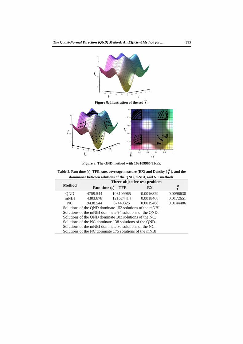
which is plotted in Figure.8. The problem is solved by the QND, the
mNBI, and NC methods with 115
for producing 256 NDPs on the real
NDF.
The convergence to the NDF and also the distribution of solutions of
the QND, mNBI, and NC methods for finding 256, NDP after
103109965, 121624414 and 87449325 TFE for the current problem are
illustrated in Figures.9-11, respectively. Results of the proposed
method are listed in Table 2.

394 (IJMS) Vol. 12, No. 3, Summer 2019
2f
1x2x
3x
Pareto front (PF) Pareto set (PS) by QND method
1f
Pareto points obtained by QND method
Figure 5. The QND method with 96226264 TFEs, fo instance, F5 test problem (Zhang, et al., 2008).
2f3x
Pareto front (PF) Pareto set (PS) by mNBI method
1f
Pareto points obtained by mNBI method
2x1x
Figure 6. The mNBI method with 399216845 TFEs, for instance, F5 test problem
(Zhang, et al., 2008).
2f 3x
Pareto front (PF) Pareto set (PS) by NC method
1f
Pareto points obtained by NC method
2x1x
Figure 7. The NC method with 10567553 TFEs, for instance, F5 test problem (Zhang, et
al., 2008).
Answers achieved by QND approach dominated 152 and 183 answers
obtained by the mNBI and NC. Also, from this number of comparisons,
answers achieved by the mNBI and NC approaches dominated 94 and
138 solutions obtained by the QND method.
Table 2 demonstrates that the solution distributions of the QND method
are better than those of the mNBI and NC methods.
The Quasi-Normal Direction (QND) Method: An Efficient Method for… 395
1f2f
3f
Figure 8: Illustration of the set Y .
3f
2f1f
2f3f
1f
Figure 9. The QND method with 103109965 TFEs.
Table 2. Run time (s), TFE rate, coverage measure (EX) and Density ( ), and the
dominance between solutions of the QND, mNBI, and NC methods.
Method Three-objective test problem
Run time (s) TFE EX
QND
mNBI
NC
4759.544
4303.678
9438.544
103109965
121624414
87449325
0.0016829
0.0018468
0.0019468
0.0096630
0.0172651
0.0144486
Solutions of the QND dominate 152 solutions of the mNBI.
Solutions of the mNBI dominate 94 solutions of the QND.
Solutions of the QND dominate 183 solutions of the NC.
Solutions of the NC dominate 138 solutions of the QND.
Solutions of the mNBI dominate 80 solutions of the NC.
Solutions of the NC dominate 175 solutions of the mNBI.

396 (IJMS) Vol. 12, No. 3, Summer 2019
3f
2f 1f2f3f
1f
Figure 10. The mNBI method with 121624414 TFEs.
3f
2f1f
2f3f
1f
Figure 11. The NC method with 87449325 TFEs.
Application to HCM for IMRT treatment planning (Craft, et al.,
2007)
As is proposed in the introduction of the current manuscript, there are a
number of multi-criteria structure problems in engineering, economic
and management applications which are often viewed as an SOP. An
example of this is found in IMRT in which the main goal of the doctor
is to destroy or reduce the tumor and at the same time to leave the
surrounding healthy tissues untouched (see Alber and Reemtsen, 2007;
Cotrutz, et al., 2001; Ehrgott and Burjony, 2001, for discussion). IMRT
is multi-objective; that is to say, for this problem there exist more than
one competing criteria which must be optimized at the same time.
For this paper, the QND algorithm proposed in the current
manuscript has been applied to solve such bi-objective problems of PC.

The Quasi-Normal Direction (QND) Method: An Efficient Method for… 397
With an available solution set as such, the therapist can juxtapose the
criteria values of several answers and base the resulted decisions on
knowledge. According to Eichfelder (2014), the cancer tumor can be
radiated by five streams with equal distances, which includes a
compilation of 400 distinctly suppressible pencil beams. If the radiation
structure is immovable and the researcher concentrates on an
optimization of the radiation strength, that part of the patient’s body
affected by the beams can be sketched by a system. According to the
thickness of the slivers of the CT-slices in such experiments, the body
of the patient is anatomized in voxels jv , 1, ,25787j . As the
researcher might face a lot of voxels, he can reduce this by applying a
clustering method proposed by Küfer, et al. (2003) that results in 8577
clusters. This has the same radiation stress with respect to a one-
radiation unit. Such clusters are denoted as 1 8577, ,c c . As is indicated
in figure 12 below, in the case study of the current manuscript, 0 1,B B
represent the tumor, 2B represents the rectum, 3B and 4B represent the
hip-bones in both sides of the body, respectively, 5B represents the other
tissues, and finally 6B represents the bladder.
Küfer et al. (2003) proposed that under radiation, 6B and 2B are the
most susceptible organs in receiving the radiation doses. Moreover, the
sparing of 6B leads to a high dose 2B and vice versa. The emission of
the stream iB , 1, ,200i to the clusters jc , 1, ,8577j
demonstrated by the matrix 8577 200jiA a
. Let
200x R be the strong
form of the stream. Then, jA x with jA the j th row of the matrix A
depicts the radiation dosage in the jc , caused by the stream iB , for the
behavior scheme x . According to Brahme (1984), in order to compare
the radiation stress in the organs, the researcher has to use the EUD.

398 (IJMS) Vol. 12, No. 3, Summer 2019
3B6
B
1B
2B
4B
5B
Target prostate
Organsat Risk
Figure 12. Schematic axial body cut.
According to Nimierko’s EUD (Niemierko, 1997) and using p -
norm such as clustered voxels, the following formula can be considered:
1( ) .( ) , 2, ,6k
k
j k
AAk j j
k j c B
D x c A x kB
(12)
The disparity of the variable dose in a part from the appropriated
perimeter kU is counted by1
( ) ( ) 1k k
k
L x D xU
. The number of voxels
in the organ kB and cluster jc are demonstrated by kV and jc ,
respectively. It is notable that | j k
j k
j c B
c B
. The results of the case
study of the current manuscript are presented in Table 3 below. The
main purpose of the current study is reduced 2B and 6B .
In this case, we will have the following bi-objective problem:
6
2
0 0 0 0 0
1 1 1 1
min ( ),
min ( )
. . ( ( ) 1) , 2,...,6
(1 ) (1 ), such that
(1 ) (1 ), such that
k k k
j j
j j j
L x
L x
s t U L x Q k
A x j c B
A x j c B
(13)
The required values are specified in Table 4.
Table 3. Pivotal rates in the part at risk.
Number of organs (k) kA kU kQ
kB
B2 2 3.0 34 36 5750
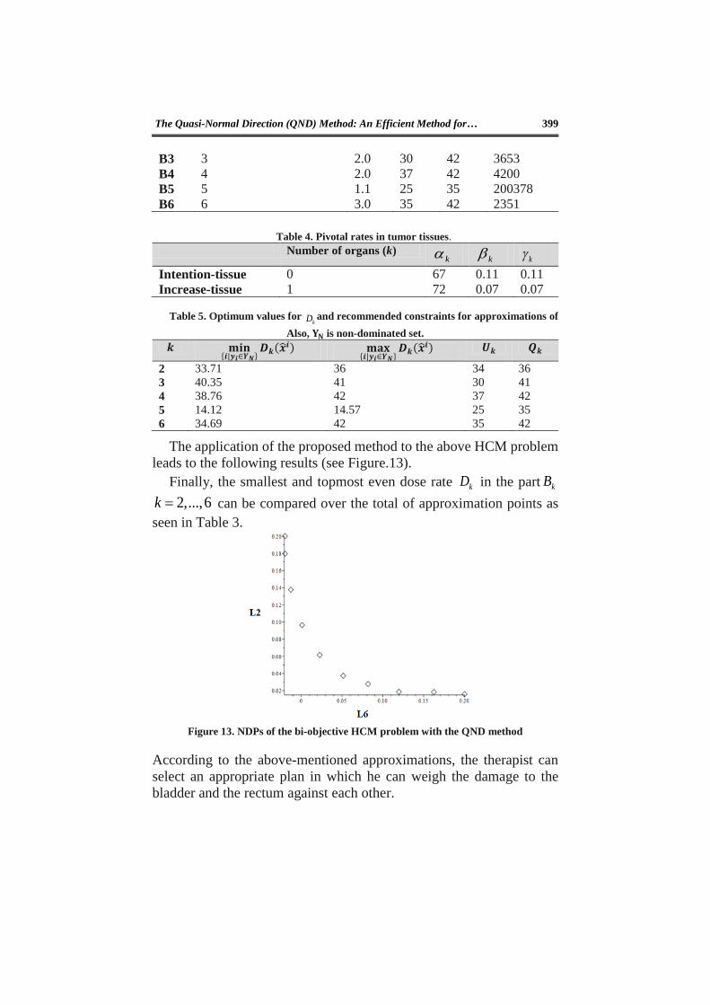
The Quasi-Normal Direction (QND) Method: An Efficient Method for… 399
B3 3 2.0 30 42 3653
B4 4 2.0 37 42 4200
B5 5 1.1 25 35 200378
B6 6 3.0 35 42 2351
Table 4. Pivotal rates in tumor tissues.
Number of organs (k) k k k
Intention-tissue 0 67 0.11 0.11
Increase-tissue 1 72 0.07 0.07
Table 5. Optimum values for kD and recommended constraints for approximations of
Also, 𝐘𝐍 is non-dominated set.
𝒌 𝐦𝐢𝐧{𝒊|𝒚𝒊∈𝒀𝑵}
𝑫𝒌(𝒙𝒊) 𝐦𝐚𝐱
{𝒊|𝒚𝒊∈𝒀𝑵}𝑫𝒌(𝒙
𝒊) 𝑼𝒌 𝑸𝒌
2 33.71 36 34 36
3 40.35 41 30 41
4 38.76 42 37 42
5 14.12 14.57 25 35
6 34.69 42 35 42
The application of the proposed method to the above HCM problem
leads to the following results (see Figure.13).
Finally, the smallest and topmost even dose rate kD in the part kB
2,...,6k can be compared over the total of approximation points as
seen in Table 3.
Figure 13. NDPs of the bi-objective HCM problem with the QND method
According to the above-mentioned approximations, the therapist can
select an appropriate plan in which he can weigh the damage to the
bladder and the rectum against each other.

400 (IJMS) Vol. 12, No. 3, Summer 2019
Conclusions
In this paper, an efficient numerical method for solving MCOPs
based on PS scalarization has been presented. The method produces
a fine representation of the whole NDF for MCOPs. The introduced
approach was applied to two problems and performed very well in
terms of constructing the NDF. The algorithm was also applied to a
HCM case study problem to demonstrate its applicability in practical
problems.
In the current study, an optimized treatment plan for radiating a
cancer tumor has been proposed. In this plan, besides getting rid of
or weakening the cancer tumor, the least possible hazards and
damages to the healthy organs of the body have been witnessed.
Moreover, an optimized medicine plan for utmost impact on control
and overcoming cancer tumors around healthy body organs is
necessary.
Use of high doses of radiation leads to the side-effects in rectum
and bladder, which is due to the high-range medicine pull of these
organs. In the current study, minimizing the medicine pull in the
bladder and the rectum was an aim. For this, a treatment plan is
achieved by the physician in which the least suffering will happen in
the patients’ bladder and the rectum during the treatment process.
In the section on numerical examples, the results of the
simulations showed that the time of performing the NC method was
less than the mNBI and QND methods, which is due to the structure
of the NC method, which is based on limiting the search space for
the answer; this is contrary to the mNBI and QND methods that are
gradient-oriented and do not limit the solution search space. As a
result, it seems obvious that the computational complication of the
NC approach is not worse than those of the other two approaches.
On the other hand, the main criterion in the quality of NDP is its
quality; examining the numbers in Tables 1 through 5 shows the
superiority of the QND method. This indicates that the QND method
has produced more high-quality responses than the other two
methods, which firstly present a greater and better spread of the
NDF, and secondly the distribution of responses is closer to the
uniform distribution and can satisfy the demand of the decision-
maker at any desired level. The results of the numerical simulations
indicate that most of the QND solutions are superior to the solutions
obtained from the other two methods and overcome them often. This

The Quasi-Normal Direction (QND) Method: An Efficient Method for… 401
suggests that the QND method approximates the NDF with more
details and less error compared with the other two methods. Along
with all the qualities of the QND method, one of the disadvantages
of it is the nonlinear structure of the method that leads to an increase
in the computational complexity observed in the examples.

402 (IJMS) Vol. 12, No. 3, Summer 2019
References
Abo-Sinna, M., Abo-Elnaga, Y. Y., and Mousa, A. (2014). An
interactive dynamic approach based on hybrid swarm
optimization for solving multiobjective programming problem
with fuzzy parameters. Applied Mathematical Modelling, 38(7-
8), 2000-2014.
Alber, M., and Reemtsen, R. (2007). Intensity modulated
radiotherapy treatment planning by use of a barrier-penalty
multiplier method. Optimisation Methods and Software, 22(3),
391-411.
Audet, C., Savard, G., and Zghal, W. (2008). Multiobjective
optimization through a series of single-objective formulations.
SIAM Journal on Optimization, 19(1), 188-210.
Brahme, A. (1984). Dosimetric precision requirements in radiation
therapy. Acta Radiologica: Oncology, 23(5), 379-391.
Cotrutz, C., Lahanas, M., Kappas, C., and Baltas, D. (2001). A
multiobjective gradient-based dose optimization algorithm for
external beam conformal radiotherapy. Physics in Medicine and
Biology, 46(8), 2161.
Craft, D., Halabi, T., Shih, H. A., and Bortfeld, T. (2007). An
approach for practical multiobjective IMRT treatment planning.
International journal of radiation oncology* Biology* Physics,
69(5), 1600-1607.
Deb, K. (2001). Multi-objective optimization using evolutionary
algorithms (Vol. 16). John Wiley and Sons.
Ehrgott, M., and Burjony, M. (2001). Radiation therapy planning
by multicriteria optimization. In Proceedings of the 36th Annual
Conference of the Operational Research Society of New
Zealand (pp. 244-253).
Eichfelder, G. (2008). Adaptive scalarization methods in
multiobjective optimization (Vol. 436). Berlin: Springer.
Eichfelder, G. (2009). Scalarizations for adaptively solving multi-
objective optimization problems. Computational Optimization
and Applications, 44(2), 249.
Eichfelder, G. (2014). Vector optimization in medical engineering
Mathematics Without Boundaries (pp. 181-215). Springer, New
York, NY.
Kasimbeyli, R., Ozturk, Z. K., Kasimbeyli, N., Yalcin, G. D., and
Erdem, B. I. (2017). Comparison of Some Scalarization Methods

The Quasi-Normal Direction (QND) Method: An Efficient Method for… 403
in Multiobjective Optimization. Bulletin of the Malaysian
Mathematical Sciences Society, 1-31.
Küfer, K.-H., Scherrer, A., Monz, M., Alonso, F., Trinkaus, H.,
Bortfeld, T., and Thieke, C. (2003). Intensity-modulated
radiotherapy–a large scale multi-criteria programming problem.
OR spectrum, 25(2), 223-249.
Lopeza, R. H., Rittob, T., Sampaioc, R., and de Cursid, J. E. S.
(2013). A new multiobjective optimization algorithm for
nonconvex pareto fronts and objective functions. Asociación
Argentina de Mecánica Computacional, 669-679.
Meng, H.-y., Zhang, X.-h., and Liu, S.-y. (2005). In International
Conference on Natural Computation (pp. 1044-1048). Springer,
Berlin, Heidelberg.
Messac, A., Ismail-Yahaya, A., and Mattson, C. A. (2003). The normalized
normal constraint method for generating the Pareto frontier. Structural
and Multidisciplinary Optimization, 25(2), 86-98.
Messac, A., and Mattson, C. A. (2004). Normal constraint method
with guarantee of even representation of complete Pareto
frontier. AIAA journal, 42(10), 2101-2111.
Niemierko, A. (1997). Reporting and analyzing dose distributions:
a concept of equivalent uniform dose. Medical physics, 24(1),
103-110.
Pardalos, P. M., Žilinskas, A., and Žilinskas, J. (2017). Non-convex
multi-objective optimization. Springer International Publishing.
Pintér, J. D., Linder, D., and Chin, P. (2006). Global Optimization
Toolbox for Maple: An introduction with illustrative
applications. Optimisation Methods and Software, 21(4), 565-
582.
Shukla, P. K. (2007). On the normal boundary intersection method
for generation of efficient front. In International Conference on
Computational Science (pp. 310-317). Springer, Berlin,
Heidelberg.
Siddiqui, S., Azarm, S., and Gabriel, S. (2011). A modified Benders
decomposition method for efficient robust optimization under
interval uncertainty. Structural and Multidisciplinary
Optimization, 44(2), 259-275.
Uilhoorn, F. E. (2017). Comparison of Bayesian estimation
methods for modeling flow transients in gas pipelines. Journal
of Natural Gas Science and Engineering, 38:159– 170.
Valipour, E., Yaghoobi, M., and Mashinchi, M. (2014). An iterative

404 (IJMS) Vol. 12, No. 3, Summer 2019
approach to solve multiobjective linear fractional programming
problems. Applied Mathematical Modelling, 38(1), 38-49.
Zhang, Q., Zhou, A., Zhao, S., Suganthan, P. N., Liu, W., and
Tiwari, S. (2008). Multiobjective optimization test instances for
the CEC 2009 special session and competition. University of
Essex, Colchester, UK and Nanyang technological University,
Singapore, special session on performance assessment of multi-
objective optimization algorithms.