the qft notes iii - homepages.dias.ie
TRANSCRIPT
THE QFT NOTES III
Badis Ydri
Department of Physics, Faculty of Sciences, Annaba University,
Annaba, Algeria.
April 9, 2011
Contents
1 CHAPTER 1:Basic Notions and Formalism of Quantum Mechanics 4
1.1 Canonical Quantization . . . . . . . . . . . . . . . . . . . . . . . . . . . . . . . . 4
1.2 Hilbert Spaces . . . . . . . . . . . . . . . . . . . . . . . . . . . . . . . . . . . . . 6
1.3 Continous Spectra and Wave Functions . . . . . . . . . . . . . . . . . . . . . . . 9
1.4 Measurement and Statistical Interpretation . . . . . . . . . . . . . . . . . . . . . 13
1.5 Set 1 . . . . . . . . . . . . . . . . . . . . . . . . . . . . . . . . . . . . . . . . . . 16
1.6 Solution 1 . . . . . . . . . . . . . . . . . . . . . . . . . . . . . . . . . . . . . . . 18
2 CHAPTER 2:Some Exact Solutions of The Schrodinger Equation 22
2.1 Stationary States . . . . . . . . . . . . . . . . . . . . . . . . . . . . . . . . . . . 22
2.2 The Free Particle . . . . . . . . . . . . . . . . . . . . . . . . . . . . . . . . . . . 23
2.3 The Harmonic Oscillator . . . . . . . . . . . . . . . . . . . . . . . . . . . . . . . 25
2.4 Scattering versus Bound States . . . . . . . . . . . . . . . . . . . . . . . . . . . 27
2.5 The Delta-Function Potential . . . . . . . . . . . . . . . . . . . . . . . . . . . . 28
2.6 The Square Potential . . . . . . . . . . . . . . . . . . . . . . . . . . . . . . . . . 31
2.7 Set 2 . . . . . . . . . . . . . . . . . . . . . . . . . . . . . . . . . . . . . . . . . . 35
2.8 Solution 2 . . . . . . . . . . . . . . . . . . . . . . . . . . . . . . . . . . . . . . . 37
3 CHAPTER 3:Notes on the Theory of Angular Momentum 39
3.1 Angular Momentum Algebra . . . . . . . . . . . . . . . . . . . . . . . . . . . . . 39
3.2 Spherical Harmonics . . . . . . . . . . . . . . . . . . . . . . . . . . . . . . . . . 42
3.3 Central Potentials-Hydrogen Atom . . . . . . . . . . . . . . . . . . . . . . . . . 44
3.4 Set 3 . . . . . . . . . . . . . . . . . . . . . . . . . . . . . . . . . . . . . . . . . . 49
3.5 Solution 3 . . . . . . . . . . . . . . . . . . . . . . . . . . . . . . . . . . . . . . . 50
1
4 CHAPTER 4:Perturbation Theory 53
4.1 Nondegenerate Perturbation Theory . . . . . . . . . . . . . . . . . . . . . . . . . 53
4.2 Degenerate Perturbation Theory . . . . . . . . . . . . . . . . . . . . . . . . . . . 55
4.3 The Fine Structure of Hydrogen . . . . . . . . . . . . . . . . . . . . . . . . . . . 57
4.4 Set 4 . . . . . . . . . . . . . . . . . . . . . . . . . . . . . . . . . . . . . . . . . . 63
4.5 Solution 4 . . . . . . . . . . . . . . . . . . . . . . . . . . . . . . . . . . . . . . . 67
5 CHAPTER 5: Scattering Theory 75
5.1 Classical Scattering Theory . . . . . . . . . . . . . . . . . . . . . . . . . . . . . 75
5.1.1 The 2−Body Central Force Problem . . . . . . . . . . . . . . . . . . . . 75
5.1.2 Differential Cross-Section . . . . . . . . . . . . . . . . . . . . . . . . . . . 78
5.1.3 Rutherford Scattering . . . . . . . . . . . . . . . . . . . . . . . . . . . . 79
5.2 Quantum Scattering Theory . . . . . . . . . . . . . . . . . . . . . . . . . . . . . 80
5.2.1 Lippmann-Schwinger Equation . . . . . . . . . . . . . . . . . . . . . . . 80
5.2.2 The Born Approximation . . . . . . . . . . . . . . . . . . . . . . . . . . . 84
5.2.3 Transition Operator . . . . . . . . . . . . . . . . . . . . . . . . . . . . . 85
5.3 Method of Phase Shifts . . . . . . . . . . . . . . . . . . . . . . . . . . . . . . . . 86
5.3.1 Schrodinger Equation in the Region V = 0 . . . . . . . . . . . . . . . . . 86
5.3.2 Plane and Spherical Waves . . . . . . . . . . . . . . . . . . . . . . . . . . 88
5.3.3 Partial-Wave Amplitudes and Phase Shifts . . . . . . . . . . . . . . . . . 90
5.4 Summary . . . . . . . . . . . . . . . . . . . . . . . . . . . . . . . . . . . . . . . 94
5.5 Set 5 . . . . . . . . . . . . . . . . . . . . . . . . . . . . . . . . . . . . . . . . . . 98
5.6 Solution 5 . . . . . . . . . . . . . . . . . . . . . . . . . . . . . . . . . . . . . . . 100
6 CHAPTER 6: Time-Dependent Perturbation Theory 105
6.1 The Dirac Interaction Picture . . . . . . . . . . . . . . . . . . . . . . . . . . . . 105
6.2 Two-State Problems . . . . . . . . . . . . . . . . . . . . . . . . . . . . . . . . . 106
6.3 Dyson Series . . . . . . . . . . . . . . . . . . . . . . . . . . . . . . . . . . . . . . 108
6.4 Fermi’s Golden Rule . . . . . . . . . . . . . . . . . . . . . . . . . . . . . . . . . 110
6.5 Emission and Absorption of Radiation . . . . . . . . . . . . . . . . . . . . . . . 112
6.5.1 Harmonic Perturbation . . . . . . . . . . . . . . . . . . . . . . . . . . . . 112
6.5.2 Stimulated Emission and Absorption . . . . . . . . . . . . . . . . . . . . 114
6.6 Set 6 . . . . . . . . . . . . . . . . . . . . . . . . . . . . . . . . . . . . . . . . . . 117
6.7 Solution 6 . . . . . . . . . . . . . . . . . . . . . . . . . . . . . . . . . . . . . . . 119
A Mid-Term Exam 3 - Take Home 125
B Mid-Term Exam 4 127
C Extra Problems 129
D Examen Final de Mecanique Quantique Avancee 131
2

E Examen Rattrapage de Mecanique Quantique Avancee 133
3
1 CHAPTER 1:Basic Notions and Formalism of Quan-
tum Mechanics
1.1 Canonical Quantization
We consider a particle moving in three dimensions in a potential V . In classical mechanics
the state of the particle is given by the point (~x, ~p) in phase space where ~x is the vector position
of the particle and ~p is the vector momentum of the particle, i.e ~p = m~x. The xi and pi are
obtained from Hamilton’s equations of motion
pi = −∂H∂xi
, xi =∂H
∂pi. (1)
The quantities (xi, pi) are called canonical variables. The H is a function on the phase space,
i.e H = H(xi, pi) known as the Hamiltonian which in this case can be identified with the total
energy. Thus
H = T + V =
∑
i pipi2m
+ V (xi). (2)
In classical mechanics a related description is given in terms of Poisson brackets. The
Poisson bracket of any two functions u and v with respect to the canonical variables xi and piis defined by
[u, v]P.B =∑
i
(
∂u
∂xi
∂v
∂pi− ∂u
∂pi
∂v
∂xi
)
. (3)
The fundamental Poisson brackets are given by
[xi, xj ]P.B = 0 , [pi, pj]P.B = 0 , [xi, pj]P.B = δij . (4)
Let Q be some function of the canonical variables xi, pi and time, i.e Q = Q(xi, pi, t). The total
time derivative of Q is given by
dQ
dt= [Q,H ]P.B +
∂Q
∂t. (5)
This is the equation of motion of the function Q. Hamilton’s equations can be obtained as a
special case. Indeed if we choose Q = xi, pi then xi = [xi, H ]P.B, pi = [pi, H ]P.B.
The quantization of the above system according to Dirac can be obtained by replacing the
Poisson brackets by commutators as follows
[, ]P.B −→ 1
ih[, ]. (6)
This is the correspondence principle. In other words we replace the coordinates xi by position
operators xi and the momenta pi by momentum operators pi such that the fundamental Poisson
brackets between xi and pi become given by the commutators
[xi, xj ] = 0 , [pi, pj] = 0 , [xi, pj]P.B = ihδij . (7)
4
These are called the canonical or fundamental commutation relations. The commutator [A,B]
is defined by A.B − B.A. Further since xi and pi are operators not numbers they must act on
some space H which is known as a Hilbert space. A Hilbert space is a complex vector space
which can be (and in this case is) infinite dimensional.
By analogy with the classical Hamiltonian which is a function of xi and pi the quantum
Hamiltonian H will be a function of xi and pi obtained as follows. Since the xi commute
among themselves and since the pi commute among themselves the quantum Hamiltonian is an
operator acting on the Hilbert space H given by
H =
∑
i p2i
2m+ V (xi). (8)
Similarly any function of the phase space coordinates Q = Q(xi, pi) will be replaced by an
operator Q = Q(t) acting on the Hilbert space H with time evolution given by the quantum
analogue of the equation of motion (5) which is obtained via the quantization prescription (6),
namely
ihdQ
dt= [Q, H]. (9)
This is Heisenberg’s equation of motion. As we will see this equation is completely equivalent
to Schrodinger’s equation. Let us introduce the unitary operator U = U(t, t0) on the Hilbert
space H, i.e U is an operator on H which satisfies UU+ = U+U = 1. The operator U will
depend on time such that
Q(t) = U(t, t0)Q(t0)U(t, t0)+. (10)
Clearly the operator Q(t0) is identified with Q(t) at the initial time t0. Thus Q0 does not
depend on t so that dQ(t0)dt
= 0. Further we must have [U(t0, t0), Q(t0)] = 0 for any operator
Q(t0) acting on the Hilbert space H and as a consequence U(t0, t0) = 1. The unitary operator
U(t, t0) carries the entire time dependence of Q(t). Indeed we compute from one hand
ihdQ
dt= ih
dU
dtQ0U
+ + ihUQ0dU+
dt. (11)
From the other hand we compute
[Q, H] = −HUQ0U+ + UQ0U
+H. (12)
Thus we get
ihdU
dt= −HU , ih
dU+
dt= U+H. (13)
The Hamiltonian in this case is time-independent. Thus we have
U = U(t, t0) = eihH(t−t0). (14)
5
In quantum mechanics there is a major distinction between observales which are the physical
quantities which we measure and state vectors of the system. As we already noted observables
are represented by operators acting on the Hilbert space H which are also hermitian, i.e Q+ = Q.
The state vectors are on the other hand represented by elements of the Hilbert space H and
thus observables can act on them to produce other state vectors. In Dirac’s notation we denote
the state vector of the system by the ket |ψ(t0) > which is also assumed to be normalizable,
i.e we can always choose |ψ(t0) > such that < ψ(t0)|ψ(t0 >= 1. A detailed discussion of these
issues will follow in the next sections.
In summary we have obtained observables represented by time-dependent hermitian oper-
ators Q(t) and state vectors |ψ(t0) > which are fixed in time. This is the Heisenberg picture.
In the Schrodinger picture the observables become fixed in time given by Q(t0) whereas state
vectors become dependent on time given by a state vector |ψ(t) > which at time t0 is identified
with |ψ(t0) >. In other words state vectors in the Schrodinger picture are given by
|ψ(t) >= U(t, t0)+|ψ0 > . (15)
The unitary operator U(t, t0) is known as the evolution operator. It is immediately evident
that the time evolution of the state vector |ψ(t) > is given by
ihd
dt|ψ(t) > = U+HU |ψ(t) >
= H|ψ(t) > . (16)
This is Schrodinger’s equation. Clearly the expectation values in the Heisenberg and Schrodinger
pictures are equal, viz
< ψ(t)|Q0|ψ(t) >=< ψ0|Q(t)|ψ0 > . (17)
The precise meaning of this equation will be explained in the next sections.
1.2 Hilbert Spaces
The concept of a Hilbert space plays a central role in quantum mechanics. Indeed the two
main ingredients of quantum mechanics which are state vectors and operators are intimately
related to the Hilbert space of the system. In fact the set of all state vectors constitute the
Hilbert space while observables are represented by hermitian operators acting on this Hilbert
space.
A Hilbert space H is a complex vector space which is typically infinite dimensional endowed
with an inner product. Following Dirac we will denote the vectors ~ψ of H by |ψ > and call
them kets. In a given basis which we assume for simplicity to be discrete we write the state
vectors as column vectors
|ψ >=∑
n
an|en > . (18)
6
We have denoted the elements of the basis by |en > where n can take the values from 0 to ∞.
The statement that the Hilbert space H is a complex vector space is precisely the requirement
that the components an are complex numbers.
Let |φ > be another state vector with components bn, i.e |φ >=∑
n bn|en >. The inner
product of the two kets |ψ > and |φ > denoted by < φ|ψ > is defined by
< φ|ψ >=∑
n
b∗nan. (19)
Similarly the inner product of the two kets |φ > and |ψ > denoted by < ψ|φ > is defined by
< ψ|φ >=∑
n
a∗nbn. (20)
From these definitions < φ|ψ >=< ψ|φ >∗. The inner product generalizes the scalar (dot)
product in real vector spaces.
From the above definition it is clear that the basis |en > was assumed to be orthonormal,
i.e
< en|em >= δnm. (21)
The inner product < φ|ψ > can also be thought of as the value of a linear function < φ| at the
vector |ψ > of the Hilbert space H. In other words
< φ| : H −→ C
|ψ >−→< φ|ψ > . (22)
The set of all the linear functions < φ| constitutes another Hilbert space H∗ which is dual to
H. The elements < φ| which are known in Dirac’s notation as bras are given by the row vectors
< φ| =∑
n
b∗n < en|. (23)
The set < en| is the basis in the dual Hilbert space H∗ which is dual to the basis |en >. In
a precise sense the bra is the hermitian conjugate of the ket and vice versa, i.e < φ| = (|φ >)+.
By using the condition < en|em >= δnm we can compute the components an of the state
vector |ψ >. We find
an =< en|ψ > . (24)
The expansion (18) takes then the form
|ψ >=∑
n
|en >< en|ψ > . (25)
In other words we must have the completeness relation
∑
n
|en >< en| = 1. (26)
7

The quantity |en >< en| is an operator which is given by the outer product of the ket |en >with the bra < en|.
Clearly the norm of a state vector |ψ > must be defined in terms of the inner product
< ψ|ψ > which is always a positive real number. The norm is obviously equal to√
< ψ|ψ >.
The two state vectors |ψ > and a|ψ > where a is a complex number will represent the same
physical state. In other words we can always normalize |ψ > such that < ψ|ψ >= 1. The
elements of the Hilbert space H are thus normalizable vectors, i.e
if |ψ >∈ H then < ψ|ψ ><∞. (27)
The observables of the system will be represented by hermitian operators acting on the
Hilbert space H. An operator Q acting on H is a linear transformation since it takes a state
vector |ψ > into another state vector given by Q|ψ > so Q is the map
Q : H −→ H|ψ >−→ Q|ψ > . (28)
This is linear in the sense that Q(a|ψ > +b|φ >) = aQ|ψ > +b|Q|ψ > for any complex
numbers a and b. Thus the operator Q can be represented by an infinite dimensional matrix
with components given in the basis |en > by < en|Q|em >, i.e
Q =∑
n
∑
m
< en|Q|em > |en >< em|. (29)
A hermitian operator is an operator satisfying the extra condition Q+ = Q where Q+ is the
hermitian conjugate or adjoint of Q defined by < φ|Q|ψ >=< ψ|Q+|φ >∗. In other words the
components of a hermitian operator satisfy < en|Q+|em >= (< em|Q|en >)∗. The expectation
value of Q in the state vector |ψ > is given by the inner product of Q|ψ > and |ψ >, viz
< Q >=< ψ|Q|ψ > . (30)
Since Q+ = Q the expectation value < Q > is real. The average of the outcomes of many
measurements of the operator Q done on identically prepared systems is identified with the
expectation value < Q >. Equivalently since the outcome of a measurement must be real the
expectation value of an operator representing an observable must be real and as a consequence
the operator must be hermitian.
A normalized state vector |ψ > is called an eigenvector of a hermitian operator Q with an
eigenvalue λ if
Q|ψ >= λ|ψ > . (31)
Thus the expectation value of Q in |ψ > is equal to λ. Furthermore the standard deviation of
Q in |ψ > defined by σ2 =< ψ|(Q− < Q >)2|ψ > is zero. In other words the eigenvector |ψ >
is a determinate state of the system in the sense that the outcomes of all measurements done
on an ensemble of identically prepared systems will yield the same value λ.
8
The set of all the eigenvalues of Q is called the spectrum of Q. The spectrum may be
degenerate, i.e there could be two or more eigenvectors with the same eigenvalue. In the case
of a hermitian operator with a discrete spectrum the eigenvalues are real and the eigenvectors
associated with different eigenvalues are orthogonal. Thus if |λn > are the eigenvectors of Q
corresponding to the eigenvalues λn we must have
< ψm|ψn >= δmn. (32)
In the above equation we have also assumed that the eigenvectors |ψn > are normalized. The
presence of degeneracy means that some eigenvalues correspond to degenerate subspaces. The
degenerate subspace associated with the eigenvalue λn which is also known as the eigenspace
of Q associated with λn contains all the eignvectors associated with the eigenvalue λn. We can
use the Gram-Schmidt orthogonalization procedure to construct orthogonal eigenvectors within
each eigenspace.
For a finite Hilbert space the set of all the eigenvectors |λn > of any hermitian operator Q is
complete. In other words any state vector |ψ > in the Hilbert space can be written as a linear
combination of the |λn >, viz
|ψn >=∑
n
cn|ψn > . (33)
The sum over n is now restricted to a finite set of N. The above property is equivalent to the
completeness relation∑
n
|ψn >< ψn| = 1. (34)
Again the sum over n is restricted to a finite set of N.
The proof of the property of completeness does not generalize to infinite dimensional Hilbert
spaces. However this property is essential in quantum mechanics and as a consequence we take
it as an axiom following Dirac. This means that we have to put a restriction on the class of
possible hermitian operators which can represent observables. Thus the completeness relation
(26) is actually an axiom. Similarly the completeness relation (34) with the sum over n not
restricted is also only an axiom.
1.3 Continous Spectra and Wave Functions
In the case of a hermitian operator with a continuous spectrum, i.e when the eigenvalues fill
out a continuous range the corresponding eigenvectors are not normalized. In other words the
corresponding eigenvectors are not in the Hilbert space and thus they do not represent physical
states. In this case only linear combinations of the eigenvectors may represent possible physical
state.
As an example we take the position and momentum operators xi and pi. We restrict ourselves
to one dimension. The canonical commutation relation reads
[x, p] = ih. (35)
9
The eigenvector |x > of the position operator x with eigenvalue x is defined by
x|x >= x|x > . (36)
The position operator is a hermitian operator. It is only natural to assume that the eigenvalues
of x are all strictly real. Then we compute
< x′ |x|x >= x < x
′ |x >= x′
< x′ |x > . (37)
We can immediately conclude that
< x′ |x >= δ(x
′ − x). (38)
The eigenvectors |x > are orthogonal but not normalizable. They are however Dirac normal-
izable in the sense that < x|x >= δ(0). Equation (38) can be called Dirac orthonormalization
condition. We can then derive the completeness relation
∫
dx|x >< x| = 1. (39)
Any state vector |ψ > can be expanded in the |x > basis as
|ψ >=∫
dx′
ψ(x′
)|x′
> . (40)
We compute
ψ(x) =< x|ψ > . (41)
This is the wave function of the system which corresponds to the state vector |ψ >. The
normalizability condition < ψ|ψ ><∞ becomes the square-integrability condition
< ψ|ψ >=∫
dx|ψ(x)|2 <∞. (42)
The set of all square-integrable functions ψ(x) on a given integral [a, b] constitute a Hilbert
space called L2(a, b). Let us also write the inner product of two state vectors |ψ > and |φ > in
the position basis. It reads
< φ|ψ >=∫
dxφ(x)∗ψ(x). (43)
Before we diagonalize the momentum operator p we find it very helpful to introduce the
notion of an infinitesimal translation U(dx) which is defined by
U(dx)|x >= |x+ dx > . (44)
10
The effect of U(dx) on a state vector |ψ > is
U(dx)|ψ > =∫
dx′
ψ(x′
)U(dx)|x′
>
=∫
dx′
ψ(x′
)|x′
+ dx >
=∫
dx′
ψ(x′ − dx)|x′
> . (45)
In the above equation we have assumed that the integral over x goes from −∞ to ∞. Assuming
that the translated state vector U(x)|ψ > is normalized we check that the operator U is unitary,
i.e U+U = 1. This operator also satisfies U(0) = 1, U−1(dx) = U(−dx) and U(dx1)U(dx2) =
U(dx1 + dx2). The unitary operator U(dx) can always be expanded around the identity as
U(dx) = 1 − iKdx. (46)
The hermitian operatorK which is known as the generator of translation will now be computed.
We compute
[x, U(dx)]|x >= dx|x+ dx > . (47)
This can also be written as
−i[x, K]|x >= |x > +O(dx). (48)
In other words
[x, K] = i. (49)
The generator of translation K can therefore be identified with the momentum operator p
divided by h, i.e
K =p
h. (50)
A finite translation U(x) can be constructed as follows. We consider N successive translation
U(dx). The finite translation U(x) is the composition of these N infinitesimal translations
U(dx), i.e U(x) = U(dx)U(dx)..U(dx) where we have N factors with dx = x/N . Thus U(x) =
(1 − iKdx)N = e−iKx.
Equation (45) can be put in the form
(1 − ip
hdx)|ψ >=
∫
dx′
(ψ(x′
) − dx∂ψ(x
′)
∂x′ )|x′
> . (51)
The partial derivative is used instead of the exact derivative because the state vector |ψ >
and as a consequence the wave function ψ(x) may depend on time which is here kept fixed.
Equivalently we can write
p|ψ >=∫
dx′ h
i
∂ψ(x′)
∂x′ |x′
> . (52)
11
Or
< x|p|ψ >=h
i
∂ψ(x)
∂x. (53)
Thus in the position basis the momentum operator reads
< x|p|x′
>= − hi
∂
∂x′ δ(x− x′
). (54)
Let |p > be the eigenvectors of p with eigenvalues p, namely
p|p >= p|p > . (55)
In the position basis this equation reads
h
i
∂
∂x< x|p >= p < x|p > . (56)
The solutions of this equation are of the form < x|p >= Aeip
hx with p and A complex. These
are not square-integrable functions. However for p real they are Dirac square-integrable in the
sense that
< p′ |p > =
∫ ∞
−∞dx < x|p >∗< x|p >
= |A|2∫ ∞
−∞dx ei
p−p′
hx
= |A|22πhδ(p− p′
). (57)
Thus with A = 1/√
2πh we have the eigenvectors
< x|p >=1√2πh
eip
hx. (58)
These are Dirac orthonormal states, i.e
< p′ |p >= δ(p− p
′
). (59)
Any state vector |ψ > can be expanded as
|ψ >=∫
dp < p|ψ > |p > . (60)
|ψ >=∫
dx < x|ψ > |x > . (61)
The position space wave function is ψ(x) =< x|ψ >. The momentum space wave function is
ψ(p) =< p|ψ >. They are related by
ψ(x) =∫
dp√2πh
ψ(p)eipx
h . (62)
12

ψ(p) =∫
dx√2πh
ψ(x)e−ipx
h . (63)
They are Fourier transform of each other.
The Schrodinger equation in the position space will read
< x|ih ddt|ψ(t) >=
∫
dx′
< x|H|x′
> ψ(t, x′
). (64)
Equivalently we have
ih∂
∂tψ(t, x) =
(
− h2
2m
∂2
∂x2+ V (x)
)
ψ(t, x). (65)
In above we have used the result that∫
dx′
< x|p2|x′
> ψ(t, x′
) = −h2 ∂2
∂x2ψ(t, x). (66)
1.4 Measurement and Statistical Interpretation
The two foundations of quantum mechanics are the Schrodinger equation and the statistical
interpretation. The Schrodinger equation computes the evolution of the wave function in time.
The statistical interpretation computes the probability of the different possible outcomes of any
measurement.
We are interseted in the measurement of a physical quantity Q(x, p). The correspond-
ing hermitian operator is Q = Q(x, p). We assume that Q has a discrete spectrum qn with
corresponding eigenfunctions ψn(x) =< x|ψn >. We assume that |ψn > satisfy the orthonor-
malization condition < ψm|ψn >= δmn and that they are complete∑
n |ψn >< ψn| = 1. The
wave function ψ(x) =< x|ψ > of the system can be expanded in the basis ψn(x) as
|ψ >=∑
n
cn|ψn > . (67)
Further we assume that |ψ > is normalized, viz
< ψ|ψ >= 1 ↔∑
n
|cn|2 = 1. (68)
Let us also recall that the components cn are given by
cn =< ψn|ψ > . (69)
The expectation value of the operator Q in the state |ψ > is
< Q >=< ψ|Q|ψ >=∑
n
|cn|2qn. (70)
The statistical interpretation states that the measurement of the observable Q(x, p) in the
state ψ(x) will yield the eigenvalues qn of the hermitian operator Q with probabilities given by
|cn|2 = | < ψn|ψ > |2 where |ψn > is the eigenvector of Q with eigenvalue qn.
13
As an example let us take Q = x. In this case the eigenvectors are |x > such that < x′|x >=
δ(x′−x) and
∫
dx|x >< x| = 1. The state vector |ψ > can be expanded as |ψ >=∫
dxψ(x)|x >where ψ(x) =< x|ψ >. Thus the probability of finding the system at x with error dx is given
by | < x|ψ > |2dx = |ψ(x)|2dx.Similarly if we take Q = p then we will find that the probability of finding the system with
momentum p with error dp is given by | < p|ψ > |2dp = |ψ(p)|2dp.A measurement of an observable Q(x, p) in the state ψ(x) will yield some definite eigenvalue
qn of Q. A second measurement performed immediately after the first is bound to yield the
same eigenvalue qn. This is because the wave function ψ(x) collapses under the act of the
first measurement to the eigenfunction ψn(x) corresponding to the eigenvalue qn so a repeated
measurement made quickly after the first will naturally yield the same result. In summary the
process of measurement and the subsequent collapse of the wave function is radically different
from the unitary evolution of the wave function provided by the Schrodinger equation.
The standard deviation in the measurements of any hermitian operator A in a state vector
|ψ > is given by
σ2A = < ψ|(A− < A >)2|ψ >
= < ψA|ψA > , |ψA >= (A− < A >)|ψ > . (71)
Similarly the standard deviation in the measurements of any hermitian operator B in a state
vector |ψ > is given by
σ2B = < ψ|(B− < B >)2|ψ >
= < ψB|ψB > , |ψB >= (B− < B >)|ψ > . (72)
Thus by using the Schwarz inequality we have
σ2Aσ
2B =< ψA|ψA >< ψB|ψB >≥ | < ψA|ψB > |2. (73)
We compute
< ψA|ψB >=1
2< ψ|[A, B]|ψ > +
1
2< ψ|[A− < A >, B− < B >]+|ψ > . (74)
The commutator term is pure imaginary whereas the anticommutator term is real. Thus
| < ψA|ψB > |2 =1
4| < ψ|[A, B]|ψ > |2 +
1
4| < ψ|[A− < A >, B− < B >]|ψ > |2
≥ 1
4| < ψ|[A, B]|ψ > |2. (75)
We get then the uncertainty relation
σ2Aσ
2B ≥ 1
4| < ψ|[A, B]|ψ > |2. (76)
14
For A = x and B = p we obtain σ2xσ
2p ≥ h2
4or equivalently
σxσp ≥h
2. (77)
In general there will be an uncertainty relation for every pair of incompatible observables, i.e
for every pair of observables which do not commute. Incompatible hermitian operators can not
be diagonalized simultaneously and as a consequence they do not have a common complete set
of eigenvectors. In contrast compatible hermitian operators, i.e those which commute have a
common complete set of eigenvectors.
Let us now take a time-dependent state vector |ψ(t) > evolving according to the Schrodinger
equation. The expectation value of a hermitian operator Q in |ψ(t) >, viz < Q >=<
ψ(t)|Q|ψ(t) > evolves in time according to
ihd
dt< Q >=< [Q, H] > . (78)
Now we choose in the uncertainty relation (76) the operators A = Q and B = H. Then we get
σ2Qσ
2H ≥ 1
4| < [Q, H] > |2. (79)
In other words
σQσH ≥ h
2|d < Q >
dt|. (80)
We define
σt =σQ
|d<Q>dt
|. (81)
Then we find
σtσH ≥ h
2. (82)
This is the time-energy uncertainty relation. The quantity σt is the amount of time in which
the expectation value of Q changes by one single standard deviation. Thus if the uncertainty in
the energy is made small the amount of time needed for the observable to change substantially
is very large.
15

1.5 Set 1
Problem 1:
1) Let |f > and |g > be two state vectors in a Hilbert space H. Show the Schwarz inequality
| < f |g > |2 ≤ < f |f >< g|g > . (83)
2) Show using the Schwarz inequality that the inner product < f |g > exists.
3) A Hilbert space is a complex vector space. By definition a vector space is closed under
vector addition and scalar multiplication. Thus if |f > and |g > are any two vectors in
the Hilbert space the sum |h >= |f > +|g > is also a vector in the Hilbert space. Show
that if f(x) and g(x) are square-integrable then h(x) is also square-integrable.
Problem 2:
1) The uncertainty inequality relation reads
σ2Aσ
2B ≥ 1
4| < [A, B]| > |2. (84)
Show that the necessary and sufficient condition for the inequality to hold is
(B− < B >)|ψ >= ia(A− < A >)|ψ > . (85)
The state described by the vector |ψ > is therefore a state of minimum uncertainty.
2) Find the solution of the above condition for A = x and B = p. Normalize the resulting
wave function to one. Use∫ ∞
−∞dxe−x
2
=√π. (86)
3) Find the corresponding wave function in momentum space.
4) For simplicity we consider the case < x >= 0. Determine when the particle has a well
defined momentum and when it is extremely localized in position space.
Problem 3:
1) We parameterize the wave function ψ(t, x) as ψ(t, x) =√ρe
iSh . The corresponding prob-
ability amplitude is ρ = ρ(t, x) defined by ρ = ψ∗(t, x)ψ(t, x). By inserting this ansatz in
the schrodinger equation derive the continuity equation
∂ρ
∂t+∂j
∂x= 0 (87)
Write down the probability current j in terms of ρ and S and in terms of ψ and ψ∗.
16
2) Using the continuity equation verify probability conservation,i.e
dP
dt= 0 , P =
∫ ∞
−∞ρ(t, x)dx. (88)
3) Relate < p > and d<x>dt
. What is the meaning of the probability current j.
4) Let us assume that the potential V is complex, i.e V = V0 − iΓ. Determine in this case
the rate of change dPdt
of the total probability. What does P describe.
5) What is the equation satisfied by S and what is its classical limit h −→ 0. What is the
meaning of S.
17
1.6 Solution 1
Problem 1:
1) Consider the norm of the vector |ψ >= |f > +a|g > with a = − < g|f > / < g|g >.
2) By Schwarz inequality we have | < f |g > | ≤√
< f |f >< g|g >. The integrals < f |f >=∫
dxf ∗(x)f(x), < g|g >=∫
dxg∗(x)g(x) converge to finite numbers since both f(x) and
g(x) are square-integrable. Hence the inner product < f |g >=∫
dxf ∗(x)g(x) converges
to a finite number.
3) We must show that < h|h >=∫
dxh∗(x)h(x) converges to a finite number. Again we use
Schwarz inequality.
Problem 2:
1) We have
σ2Aσ
2B =< ψA|ψA >< ψB|ψB >≥ | < ψA|ψB > |2. (89)
The equality hold if |ψB >= c|ψA >. Further we have
| < ψA|ψB > |2 =1
4| < ψ|[A, B]|ψ > |2 +
1
4| < ψ|[A− < A >, B− < B >]|ψ > |2
≥ 1
4| < ψ|[A, B]|ψ > |2. (90)
The inequality will hold if < ψ|[A− < A >, B− < B >]|ψ >= 0. This leads to the
condition (c+ c∗) < ψA|ψc >= 0, i.e c is pure imaginary. We write c = ia. The necessary
and sufficient condition is therefore
(B− < B >)|ψ >= ia(A− < A >)|ψ > . (91)
2) For A = x and B = p we obtain in the position basis the equation
(h
i
d
dx− < p >)ψ(x) = ia(x− < x >)ψ(x). (92)
We remove the plane wave behaviour from ψ(x) by writing
ψ(x) = ei<p>x
h φ(x). (93)
We get a differential equation for φ(x) given by
d lnφ
dx= −a
h(x− < x >) (94)
Thus φ is given by
φ(x) = Ae−a2h
(x−<x>)2 . (95)
18
The general minimum-uncertainty solution is the gaussian
ψ(x) = Ae−a2h
(x−<x>)2ei<p>x
h . (96)
Normalization yields the value
A = (a
hπ)
14 . (97)
3) We compute
ψ(k) =∫
dx√2πh
e−ikxh ψ(x)
= A∫
dx√2πh
e−a2h
[x− ia(<p>−k−ia<x>)]2e−
12ah
(<p>−k−ia<x>)2− a2h<x>2
= (1
πah)
14e−
12ah
(<p>−k−ia<x>)2− a2h<x>2
. (98)
4) We consider < x >= 0 for simplicity. The probability density of finding the particle with
a momentum k with error < p > is a gaussian centered in momentum space around k
given by |ψ(k)|2. The width of this gaussian is d2k = ah which is inversely proportional to
the width d2x = h/a of the gaussian ψ(x).
In the limit a −→ 0 we have dk −→ 0, i.e the wave function ψ(k) is a delta function
peaked around k. In this case dx −→ ∞ and the wave function ψ(x) is a plane wave with
momentum k.
In the limit a −→ ∞ we have dx −→ 0 and as a consequence the particle wave function
ψ(x) becomes a delta function peaked around 0, i.e the particle is well localized around
0. The momentum space wave function ψ(k) becomes on the other hand a constant
independent of k.
Problem 3:
1) We parameterize the wave function ψ(t, x) as
ψ(t, x) =√ρe
iSh . (99)
The corresponding probability amplitude is ρ = ρ(t, x) defined by
ρ = ψ∗(t, x)ψ(t, x). (100)
Inserting this ansatz in the schrodinger equation we obtain
√ρ[
1
2m(∂S
∂x)2 + V +
∂S
∂t
]
− h2
2m
∂2√ρ∂x2
= ih[
∂√ρ
∂t+
1
m
∂√ρ
∂x
∂S
∂x+
1
2m
√ρ∂2S
∂x2
]
=ih
2√ρ
[
∂ρ
∂t+∂j
∂x
]
. (101)
19

The probability current is defined by
j =1
mρ∂S
∂x. (102)
We can check that
j =h
2im[ψ∗∂ψ
∂x− ψ
∂ψ∗
∂x]. (103)
It is clear that the right-hand side of equation (101) is pure imaginary while the left-hand
side is real. Thus both sides must vanish identically separately. We get therefore from
the vanishing of the right-hand side the continuity equation
∂ρ
∂t+∂j
∂x= 0. (104)
2) This expresses probability conservation. Indeed we compute
dP
dt=
∫
dx∂ρ
∂t
= −∫
dx∂j
∂x= j(t,−∞) − j(t,+∞). (105)
Since the wave function ψ(t, x) is square-integrable we must have ψ −→ 0 and ∂ψ∂x
−→ 0
as x −→ ±∞. Thus j(t, x) −→ 0 as x −→ ±∞, i.e dPdt
= 0.
3) The probability current j is in some sense the velocity of the particle. Indeed we compute
from one hand∫
j(t, x)dx =< p >
m. (106)
We compute from the other hand
< p >
m=d < x >
dt. (107)
This last equation is an example of Ehrenfest’s theorem that expectation values of quan-
tum operators follow classical laws.
4) In the case of a complex potential V = V0 − iΓ we compute
ihdP
dt= ih
∫ (
∂ψ∗
∂t.ψ + ψ∗.
∂ψ
∂t
)
dx
=∫ (
(−V ∗ψ∗).ψ + ψ∗.(V ψ))
dx
= −2iΓP. (108)
Thus
dP
dt= −2Γ
hP , P = P0e
− 2Γht. (109)
This equation describes the spontaneous decay of an unstable particle with lifetime τ = h2Γ
.
20
5) By setting the left-hand side of equation (101) equal to 0 we get the quantum Hamilton-
Jacobi equation. This is given by
[
1
2m(∂S
∂x)2 + V +
∂S
∂t
]
− h2
2m
∂2√ρ∂x2
= 0. (110)
In the limit h −→ 0 this equation becomes exactly the Hamilton-Jacobi equation. From
classical mechanics we know that S is the action of the system and thus ∂S∂x
is indeed the
momentum.
21
2 CHAPTER 2:Some Exact Solutions of The Schrodinger
Equation
2.1 Stationary States
The Schrodinger equation reads
ih∂
∂tΨ(t, x) =
(
− h2
2m
∂2
∂x2+ V (x)
)
Ψ(t, x). (111)
For a given potential V what are the solutions ψ(t, x). This is the problem we would like to
solve in general. We start with a separation of variables
Ψ(t, x) = ψ(x)φ(t). (112)
We get
ih
φ
dφ
dt=
1
ψ
(
− h2
2m
d2
dx2+ V (x)
)
ψ. (113)
The left-hand side is a function of t only while the right-hand side is a function of x only. Thus
both sides must be equal to a constant E independent of t and x. We have then
dφ
dt= −iE
hφ −→ φ(t) = e−i
Eth . (114)
The other equation reads(
− h2
2m
d2
dx2+ V (x)
)
ψ = Eψ. (115)
The constant E must therefore be real since it is nothing but the eigenvalue of the Hamiltonian
H = − h2
2md2
dx2 + V (x) with eigenfunction ψ(x). In other words the separable solution Ψ(t, x) =
e−iEth ψ(x) is a determinate solution of definite energy equal E.
Further this solution is stationary since the probability density is independent of time, i.e
ρ = Ψ∗(t, x)Ψ(t, x) = ψ∗(x)ψ(x). In fact the expectation value of every observable Q(x, p) is
independent of time. Indeed
< Q >=< Ψ|Q|Ψ > =∫
dxΨ∗(t, x)Q(x,h
i
∂
∂x)Ψ(t, x)
=∫
dxψ(x)Q(x,h
i
d
dx)ψ(x). (116)
Let ψn(x) be the eigenfunctions of the Hamiltonian H with eigenvalues En. The general solu-
tion of the Schrodinger equation is a linear combination of the separable solutions Ψn(t, x) =
e−iEnt
h ψn(x). This is given by
Ψ(t, x) =∑
n
cnψn(x)e−iEnt
h . (117)
This is the principle of quantum superposition. The coefficients cn must be determined from
the initial condition
Ψ(0, x) =∑
n
cnψn(x). (118)
22
2.2 The Free Particle
In the case the potential is zero everywhere. The time-independent Schrodinger equation
reads
− h2
2m
d2ψ
dx2= Eψ. (119)
This we rewrite as
d2ψ
dx2= −k2ψ , k2 =
2mE
h2 . (120)
This way of writing suggests that there is a solution only for E ≥ 0. In fact E is the kinetic
energy of the particle T = 12mv2 = p2
2m. The velocity and the momentum of the particle are
thus given by
v =
√
2E
m=
p
m, p = hk. (121)
The general solution of the time-independent Schrodinger equation is
ψ(x) = Aeikx +Be−ikx. (122)
Multiplying by the time-dependent phase factor e−iEth we obtain
Ψ(t, x) = Aeikh(x−vphaset) +Be−i
kh(x+vphaset). (123)
The first term represents a wave travelling to the right at speed vphase whereas the second term
represents a wave travelling to the left at speed vphase. The phase velocity is given by
vphase =E
hk=
p
2m=
1
2v. (124)
We can write the above solution in the equivalent form
Ψk(t, x) = Aei(kx−hk2
2mt). (125)
k = ±√
2mE
h. (126)
k > 0 , wave traveling to the right
k < 0 , wave traveling to the left. (127)
The first problem with these propagating solutions is that they are waves which travel at half
the speed of the particle. The second problem consists in the fact that these solutions are not
renormalizable. Thus there is no free particle with definite value of the momentum.
23
The general solution to the Schrodinger equation can be obatined as a linear combination
of the separable stationary solutions Ψk(t, x), namely
Ψ(t, x) =∫ ∞
−∞
dk√2π
φ(k)
AΨk(t, x)
=∫ ∞
−∞
dk√2πφ(k)ei(kx−
hk2
2mt). (128)
This wave function can be normalized for appropriate choices of the functions φ(k). It is called
a wave packet. The functions φ(k) can be determined from the initial condition
Ψ(0, x) =∫ ∞
−∞
dk√2πφ(k)eikx. (129)
The solution is given by Plancherel’s theorem, i.e φ(k) is the Fourier transform of Ψ(0, x) which
is given by
φ(k) =∫ ∞
−∞
dx√2π
Ψ(0, x)e−ikx. (130)
Let us remark that∫
dxΨ∗(t, x)Ψ(t, x) =∫
dxΨ∗(0, x)Ψ(0, x) =∫
dkφ∗(k)φ(k). (131)
It remains to verify that the velocity of the wave packet is equal to the velocity of the particle
v. The velocity of the wave packet is known as the group velocity and it can be greater than,
equal to or less than the phase velocity. We will consider a general wave packet given by
Ψ(t, x) =∫ ∞
−∞
dk√2πφ(k)ei(kx−ωt). (132)
We will also assume a general dispersion relation. In other words we take the angular frequency
ω to be a general function of k, i.e ω = ω(k). Further we will assume that φ(k) is peaked around
some value k = k0 so that the different components of the wave packet travel at almost the
same phase velocity vphase = ω/k and as a consequence the shape of the wave packet changes
very slowly. In fact it is only in this case that the notion of a group velocity makes a well
defined meaning. Thus we can expand ω in a Taylor series around k = k0 as
ω(k) = ω(k0) + ω′
(k0)(k − k0) + ... (133)
We compute (with k′= k − k0, ω0 = ω(k0) and ω
′
0 = ω(k0))
Ψ(t, x) = e−iω0t∫ ∞
−∞
dk′
√2πφ(k
′
+ k0)ei((k
′+k0)x−ω
′
0k′t)
= ei(−ω0+k0ω′
0)t∫ ∞
−∞
dk′
√2πφ(k
′
+ k0)ei(k
′+k0)(x−ω
′
0t). (134)
24

At time t = 0 we get
Ψ(0, x) =∫ ∞
−∞
dk′
√2πφ(k
′
+ k0)ei(k
′+k0)x. (135)
Thus
Ψ(t, x) = ei(−ω0+k0ω′
0)tΨ(0, x− ω′
0t). (136)
As desired the wave packet does not change profile and it moves with the group velocity
vgroup = ω′
0 =dω
dk|k=k0. (137)
In our case ω = hk2/2m and thus the group velocity is
vgroup =hk0
m=p0
m= v0. (138)
2.3 The Harmonic Oscillator
Let x0 be a local miminum of the potential V , i.e
V′
(x0) = 0. (139)
Further we can always choose without any loss of generality V (x0) = 0. Expanding V (x) in a
Taylor series around x0 we get
V (x) = V (x0) + (x− x0)V′
(x0) +1
2(x− x0)
2V′′
(x0) + ...
=1
2V
′′
(x0)(x− x0)2 + ... (140)
This is the potential energy of a simple harmonic oscillator with spring constant k = V′′(x0) =
mω2.
The time-independent Schrodinger equation describing the motion around the local mini-
mum x0 is then given by
(
− h2
2m
d2
dx2+
1
2mω2x2
)
ψ = Eψ. (141)
We also write this equation as
(
p2
2m+
1
2mω2x2
)
|ψ >= E|ψ > . (142)
We recall that ψ(x) =< x|ψ >. We introduce the creation and annihilation operators a+ and
a by
a+ =1√
2hmω(mωx− ip) , a =
1√2hmω
(mωx+ ip). (143)
25
Since [x, p] = ih we compute the commutation relation
[a, a+] = 1. (144)
It is straightforward to check that the Hamiltonian of the simple harmonic oscillator given by
H = p2
2m+ 1
2mω2x2 can be rewritten as
H = hω(a+a+1
2). (145)
We compute
[H, a] = −hωa , [H, a+] = hωa+. (146)
By using these equations and the time-independent Schrodinger equation H|ψ >= E|ψ > we
obtain
Ha|ψ >= (E − hω)a|ψ > , Ha+|ψ >= (E + hω)a+|ψ > . (147)
In other words a|ψ > is an eigenvector of H with eigenvalue E − hω while a+|ψ > is an eigen-
vector of H with eigenvalue E + hω. Thus a decreases the energy hence the name annihilation
or lowering operator while a+ increases the energy hence the name creation or raising operator.
Let us introduce the number operator
N = a+a. (148)
Let |n > be the eigenvectors of N with eigenvalues n, i.e
N |n >= n|n > . (149)
Since N is a hermitian operator the eigenvalues n are real and the eigenvectors |n > are
orthogonal. In fact the numbers n must be positive since n = |a|n > |2. Furthermore from the
commutation relations [N, a] = −a and [N, a+] = a+ we compute Na|n >= (n− 1)a|n > and
Na+|n >= (n+ 1)a+|n >. In other words
a|n >= cn|n− 1 > , a+|n >= dn|n+ 1 > . (150)
By requiring that the eigenvectors |n > are normalized, i.e < n|n >= 1 we obtain |cn|2 = n
and |dn|2 = n + 1. Thus by taking cn and dn to be real positive for simplicity we have
a|n >=√n|n− 1 > , a+|n >=
√n+ 1|n+ 1 > . (151)
The allowed values of the energy are therefore given by
En = hω(n+1
2). (152)
The corresponding eigenvectors are |n >.
26

We use now the general result that the energy of any normalizable solution of the time-
independent Schrodinger equation must be larger or equal than the minimum value of the
potential V .
In our case where the minimum value of V is 0 we found that the values En of the energy are
always larger than zero since n ≥ 0. Indeed the ground state energy E0 of the simple harmonic
oscillator is
E0 =1
2hω. (153)
Clearly starting from any state vector |n > we can reach the gound state vector |0 > by a
repeated application of the annihilation operator a. This means in particular that n must be
an integer since it is equal to the number of times we need to apply a to go from |n > to |0 >.
We get then the quantization condition
n ∈ N. (154)
The ground state vector |0 > must satisfy the condition a|0 >= 0. This condition reads in the
position basis as (with ψ0(x) =< x|0 >)
(d
dx+mω
hx)ψ0(x) = 0. (155)
The normalized solution is given by
ψ0(x) = (mω
πh)
14e−
mω2hx2
. (156)
The state vectors |n > can be computed in terms of |0 > as follows
|1 >= a+|0 >
|2 >=a+
√2|1 >=
(a+)2
√2!
|0 >
|3 >=a+
√3|2 >=
(a+)3
√3!
|0 >.
.
|n >=a+
√n|n− 1 >=
(a+)n√n!
|0 > . (157)
2.4 Scattering versus Bound States
We consider a particle moving in one dimension in a potential V (x). In classical mechanics
if the energy E is smaller than the values V (∞) and V (−∞) of the potential then we have a
bound state, i.e the particle can not escape the potential well to infinity. If E is larger than
V (∞) and/or V (−∞) then we have a scattering state, i.e the particle comes from infinity, it
enters the potential field then it returns back to infinity.
27
Similarly in quantum mechanics there are two possible solutions to the Schrodinger equation.
Bound states and scattering states. They are defined by
E < V (−∞) and E < V (+∞) : bound state
E > V (−∞) or E > V (+∞) : scattering state. (158)
For the harmonic oscillator we have only bound states whereas for the free particle we have
only scattering states. In most cases the potential is zero at infinity in which cases we will have
instead
E < 0 : bound state
E > 0 : scattering state. (159)
2.5 The Delta-Function Potential
The potential is given by
V (x) = −αδ(x). (160)
The constant α is positive. The time-independent Schrodinger equation reads
− h2
2m
d2ψ
dx2− αδ(x)ψ = Eψ. (161)
Bound States (E ≤ 0): Define
κ =
√−2mE
h. (162)
The time-independent Schrodinger equation becomes
d2ψ
dx2+
2mα
h2 δ(x)ψ = κ2ψ. (163)
For x < 0 or x > 0 we have
d2ψ
dx2= κ2ψ. (164)
The solution for x < 0 is of the form
ψ(x) = Ae−κx +Beκx. (165)
In the limit x −→ −∞ the above solution blows up unless A = 0. Thus we must have
ψ(x) = Beκx , x < 0. (166)
28
Similarly the solution for x > 0 is of the form
ψ(x) = Fe−κx +Geκx. (167)
Now in the limit x −→ ∞ this solution blows up unless G = 0. Thus we must have
ψ(x) = Fe−κx , x > 0. (168)
The wave function ψ(x) is always continous whereas its first derivative dψ(x)/dx is always
continous except where the potential diverges. Thus from the first boundary condition we must
have
F = B. (169)
We have then the result
ψ(x) = Be+κx , x ≤ 0
ψ(x) = Be−κx , x ≥ 0. (170)
Let us integrate the time-independent Schrodinger equation between −ǫ and +ǫ. We have
∫ ǫ
−ǫdxd2ψ
dx2= −2mα
h2
∫ ǫ
−ǫdxδ(x)ψ + κ2
∫ ǫ
−ǫdxψ. (171)
We obtain in the limit ǫ −→ 0 the result
dψ
dx|+ǫ −
dψ
dx|−ǫ = −2mα
h2 ψ(0). (172)
In other words the first derivative of the wave function is discontinuous at x = 0 precisely
because the potential diverges at this point. The above equation yields the result
−2Bκ = −2mα
h2 B. (173)
In other words
κ =mα
h2 . (174)
The energy of the bound state is therefore
E = − h2κ2
2m= −mα
2
2h2 . (175)
Normalizing the wave function ψ(x) we get B =√κ. The wave function of the bound state is
then given by
ψ(x) =√κe−κ|x|. (176)
29
Scattering States (E ≥ 0): Define
k =
√2mE
h. (177)
d2ψ
dx2+
2mα
h2 δ(x)ψ = −k2ψ. (178)
The solution for x < 0 is of the form
ψ(x) = Aeikx +Be−ikx. (179)
The solution for x > 0 is of the form
ψ(x) = Feikx +Ge−ikx. (180)
From the requirement that the wave function is continuous at x = 0 we must have
A+B = F +G. (181)
We compute the derivatives
dψ
dx|+ǫ = ik(F −G) ,
dψ
dx|−ǫ = ik(A− B). (182)
From the requirement (172) we obtain
ik(F −G− A+B) = −2mα
h2 (A +B). (183)
Equivalently
F −G = (1 + 2iβ)A− (1 − 2iβ)B , β =mα
h2k. (184)
The constants A and F are the amplitudes of waves propagating to the right whereas B and G
are the amplitudes of waves propagating to the left. In a scattering experiment particles will be
coming from one direction say the left. In this case A corresponds to incident, B corresponds
to reflected and F corresponds to transmitted waves whereas G = 0. Thus we will consider
G = 0 , scattering from left. (185)
We get then the coefficients
B =iβ
1 − iβA , F =
1
1 − iβA. (186)
Thus we get the wave functions
ψincid = Aeikx
ψrefle =iβ
1 − iβAe−ikx
ψtrans =1
1 − iβAeikx. (187)
30
The total wave functions are
ψ(x) = ψincid(x) + ψrefle(x) , x < 0. (188)
ψ(x) = ψtrans(x) , x > 0. (189)
We recall that |ψ(x)|2 is the probability of finding the particle at the point x. In other words
given an ensemble of particles all in the state ψ(x) the quantity |ψ(x)|2 will measure the fraction
of particles found at the point x. Hence∫
dx|ψincid|2 = |A|2 ∫ dx, ∫ dx|ψrefle|2 = |B|2 ∫ dx and∫
dx|ψtrans|2 = |F |2 ∫ dx are the total numbers of incident, reflected and transmitted particles
with energy E. Although these numbers are divergent since the wave functions ψincid, ψrefle and
ψtrans are not normalizable their ratios are finite.
Thus the relative probability that an incident particle will be reflected is given by the ratio
of the number of reflected particles to the number of incident particles, i.e
R =|B|2|A|2 =
β2
1 + β2=
1
1 + 2h2Emα2
. (190)
This is called the reflection coefficient which computes the fraction of incoming particles which
will be reflected. Similarly the relative probability that an incident particle will be transmitted
is given by the ratio of the number of transmitted particles to the number of incident particles,
i.e
T =|F |2|A|2 =
1
1 + β2=
1
1 + mα2
2h2E
. (191)
This is called the transmission coefficient which computes the fraction of incoming particles
which will be transmitted. We have
R + T = 1. (192)
Let us note that when E −→ ∞ we have R −→ 0 and T −→ 1. In other words particles with
sufficient energy are more likely to be transmitted.
The wave functions ψincid, ψrefle and ψtrans are not physical since they are normalizable.
These wave functions should then be replaced with normalizable wave packets as we did in the
free particle case which will necessarily involve a range of energies. We consider wave packets
which are localized around the value k of the wavenumber so that the energy will be localized
around the value E. The incident, reflected and transmitted wave packets must satisfy the
same boundary conditions satisfied by ψincid, ψrefle and ψtrans. The above analysis which was
done with ψincid, ψrefle and ψtrans will then hold only R and T will now have the interpretation
of being the reflection and transmission coefficients for particles with energy around E.
2.6 The Square Potential
We consider the potential
V = −V0 , −a < x < a
V = 0 , |x| > 0. (193)
31
Bound states (E < 0): Define
κ =
√−2mE
h. (194)
There are three regions. Region I corresponds to x < −a and region III corresponds to x > a.
In these two regions the Schrodinger equation reads
d2ψ
dx2= κ2ψ. (195)
The general solution is
ψ(x) = Ae−κx +Beκx. (196)
Clearly the solutions in region I is
ψI(x) = Beκx , x < −a. (197)
Similarly the solution in region III is given by
ψIII(x) = Fe−κx , x > a. (198)
The energy of any normalizable solution of the Schrodinger equation must be larger or equal
than the minimum value of the potential. In here this means that we must have E > −V0.
Thus in region II, i.e for −a < x < a the Schrodinger equation reads
d2ψ
dx2= −l2ψ , l =
√
2m(E + V0)
h. (199)
The solution reads
ψII(x) = C sin lx+D cos lx. (200)
Since the potential is even we can assume without any loss of generality that the wave function
is either even or odd. By assuming that it is even we can immediately set C = 0. We get
ψII(x) = D cos lx. (201)
The boundary conditions ψI(−a) = ψII(−a), ψII(a) = ψIII(a) leads to the equations
B = F. (202)
Be−κa = D cos la. (203)
The boundary conditions ψ′
I(−a) = ψ′
II(−a), ψ′
II(a) = ψ′
III(a) leads to the equation
κBe−κa = Dl sin la. (204)
32
Thus the allowed energies must satisfy the condition
tan la =κ
l. (205)
Define
z = la , z0 =a
h
√
2mV0. (206)
We remark that κ2 + l2 = 2mV0/h2 and hence a2κ2 = z2
0 − z2. Thus
tan z =
√
z20
z2− 1. (207)
This transcendental equation must be solved for the unkown z or equivalently for E as a function
of z0 which measures the size of the well.
For a wide deep well, i.e z0 −→ ∞ we have tan z −→ ∞. Hence z = nπ/2 with n odd. Thus
in this case the intersection points of the two functions tan z and√
z20
z2− 1 occur at
zn = nπ
2↔ E
′
n = En + V0 =h2π2n2
2m(2a)2. (208)
For finite V0 there are finite number of solutions. In the limit V0 −→ ∞ the values E′
n become
the values of the energy of the infinite square well.
For a shallow narrow well we will have fewer bound states. In fact for all values of z0 which
are less than π/2 no matter how small we will always have one bound state.
Scattering states (E > 0): Define
k =
√2mE
h. (209)
We have the solutions
ψI(x) = Aeikx +Be−ikx , x < −aψII(x) = C sin lx+D cos lx , −a < x < a
ψIII(x) = Feikx , x > a. (210)
In regions I and III the particle is free. The incident wave is proportional to A, the reflected
wave is proportional to B and the transmitted wave is proportional to F . The continuity of
the wave function at x = ±a leads to the equations
Ae−ika +Beika = −C sin la+D cos la
Feika = C sin la+D cos la. (211)
33
The continuity of the first derivative of the wave function at x = ±a leads to the equations
ik(Ae−ika − Beika) = l(C cos la+D sin la)
ik(Feika) = l(C cos la−D sin la). (212)
We use the second equation of (211) and the second equation of (212) to find
C = (sin la+ik
lcos la)eikaF , D = (cos la− ik
lsin la)eikaF. (213)
We substitute these expressions in the first equation of (211) and the first equation of (212) to
find
Ae−ika +Beika = (cos 2la− ik
lsin 2la)eikaF
Ae−ika − Beika = (cos 2la− il
ksin 2la)eikaF. (214)
Thus
F =e−2ika
cos 2la− ik2+l2
2klsin 2l
A. (215)
B = il2 − k2
2klsin 2laF. (216)
The transmission coefficient is
T =|F |2|A|2 =
1
cos2 2la+ (k2+l2
2kl)2 sin2 2la
. (217)
The reflection coefficient is
R =|B|2|A|2 =
(k2−l22kl
)2 sin2 2la
cos2 2la+ (k2+l2
2kl)2 sin2 2la
. (218)
We check that
R + T = 1. (219)
34
2.7 Set 2
Problem 1:
1) The two expressions D1(x) and D2(x) which involve the Dirac delta function are said to
be equal if∫ ∞
−∞dxf(x)D1(x) =
∫ ∞
−∞dxf(x)D2(x). (220)
Show that
δ(cx) =1
|c|δ(x). (221)
2) The step function θ(x) is defined by
θ(x) = 1 , x > 0
θ(x) = 0 , x < 0. (222)
Show that
dθ
dx= δ(x). (223)
Problem 2: The Plancherl’s theorem reads
f(x) =1√2π
∫ ∞
−∞F (k)eikxdk ↔ F (k) =
1√2π
∫ ∞
−∞f(x)e−ikxdx. (224)
Show that
δ(x) =1
2π
∫ ∞
−∞eikxdk. (225)
Problem 3: We consider the delta-function potential. In regions I(x < 0) and II(x > 0) the
wave functions read
ψI(x) = Aeikx +Be−ikx , x < 0
ψII(x) = Feikx +Ge−ikx , x > 0. (226)
We have two boundary conditions at x = 0 given by
F +G = A+B
F −G = A(1 + 2iβ) − B(1 − 2iβ). (227)
Thus we can solve for two of the constants in terms of the other two. We have
β =mα
h2k, k =
√2mE
h. (228)
35

1) Compute the S(cattering)-matrix S defined by
(
B
F
)
=
(
S11 S12
S21 S22
)(
A
G
)
. (229)
This gives the outgoing amplitudes B and F (i.e those moving away from the potential)
in terms of incoming amplitudes A and G (i.e those moving towards the potential).
2) Compute the T(ransfer)-matrix T defined by
(
F
G
)
=
(
T11 T12
T21 T22
)(
A
B
)
. (230)
This gives the amplitudes to the right of the potential F and G in terms of those to the
left A and B.
3) Discuss the S-matrix and T-matrix for a general potential which vanishes at x −→ ±∞.
4) For scattering from the left write down the reflection and transmission coefficients in
terms of Sij and Tij .
5) Show that for a potential consisting of two disconnected pieces the T -matrix satisfies
T = T2T1. (231)
The Ti is the T -matrix of the ith piece separately.
36
2.8 Solution 2
Problem 1:
1) We compute
∫ ∞
−∞f(x)δ(cx)dx =
∫ ∞
−∞f(y
c)δ(y)
dy
|c|
=f(0)
|c|
=1
|c|∫ ∞
−∞f(x)δ(x)dx. (232)
The absolute value comes from the integral sign. We immediately conclude that δ(cx) =1|c|δ(x).
2) We compute
∫ ∞
−∞f(x)
dθ
dxdx = [f(x)θ(x)]∞−∞ −
∫ ∞
−∞df(x)θ(x)
= [f(x)θ(x)]∞−∞ −∫ ∞
0df(x)
= f(0). (233)
Hence dθdx
= δ(x).
Problem 2: Choose f(x) = δ(x) then we will find F (k) = 1/√
2π. By substitution we
get then the desired result
δ(x) =1
2π
∫ ∞
−∞eikxdk. (234)
Problem 3:
1) We find
S =1
1 − iβ
(
iβ 1
1 iβ
)
. (235)
2) We find
T =
(
1 + iβ 1 + iβ
−iβ −iβ
)
. (236)
37

3) We still have the wave functions
ψI(x) = Aeikx +Be−ikx , x −→ −∞ψII(x) = Feikx +Ge−ikx , x −→ +∞. (237)
In region III where the potential is non-zero the wave function will be of the general form
ψIII = Cf(x) +Dg(x). (238)
The functions f and g are two linearly independent particular solutions of the Schrodinger
equation. We have two constants of integration C andD because the Schrodinger equation
is a linear second order differential equation.
We have 4 boundary conditions. There are two conditions which join regions I and III
and two conditions which join regions II and III. Two of the boundary conditions can
be used to eliminate C and D. There remains the four constants A, B, F and G. The
two remaining boundary condition can be used to determine two of the constants in term
of the other two. We can therefore define the S-matrix and T-matrix in the same way as
before.
4) First we compute
S11 = −T21
T22, S12 =
1
T22, S21 = T11 −
T12T21
T22, S22 =
T12
T22. (239)
We find for G = 0 the coefficients
Rl =|B|2|A|2 = |S11|2 = |T21
T22
|2. (240)
Tl =|F |2|A|2 = |S21|2 = |T11 −
T21T12
T22|2. (241)
5) The proof is almost obvious.
38
3 CHAPTER 3:Notes on the Theory of Angular Mo-
mentum
3.1 Angular Momentum Algebra
The angular momentum is defined by
~L = ~r × ~p. (242)
In components we have
L1 = x2p3 − x3p2 , L2 = x3p1 − x1p3 , L3 = x1p2 − x2p1. (243)
In the quantum theory we make the replacements
xi −→ xi , pi −→ pi : [xi, pj] = ihδij. (244)
Thus the angular momentum operators will be defined by
L1 = x2p3 − x3p2 , L2 = x3p1 − x1p3 , L3 = x1p2 − x2p1. (245)
We compute
[L1, L2] = x2[p3, x3]p1 + x1[x3, p3]p2
= ihL3. (246)
Similarly we compute
[L3, L1] = ihL2 , [L2, L3] = ihL1. (247)
We can write these commutation relations in a compact form as
[Li, Lj ] = ihǫijkLk (248)
This equation defines the algebra of angular momentum also called the su(2) Lie algebra. The
symbol ǫijk is the totally antisymmetric Levi-Civita tensor defined by ǫ123 = ǫ312 = ǫ231 = 1,
ǫ213 = ǫ132 = ǫ321 = −1 and ǫijk = 0 if i = j or i = k or j = k.
These commutation relations means in particular that the operators Li are incompatible
operators and thus by the uncertainty principle they can not be diagonalized simultaneously.
There is no determinate angular momentum vector. Let us defined the square of the total
angular momentum by
L2 = L21 + L2
2 + L23. (249)
39
This operator commutes with the components Li. Indeed we compute
[L2, L3] = [L21, L3] + [L2
2, L3]
= L1[L1, L3] + [L1, L3]L1 + L2[L2, L3] + [L2, L3]L2
= 0. (250)
Similarly we compute
[L2, L2] = 0 , [L2, L1] = 0. (251)
Thus we can diagonalize L2 and one of the components of the angular momentum operator say
L3. We write
L3|f >= µ|f > , L2|f >= λ|f > . (252)
We define the raising and lowering operators by
L± = L1 ± iL2. (253)
We compute the commutation relations
[L+, L−] = 2hL3 , [L3, L±] = ±hL± , [L2, L±] = 0. (254)
Thus
L3(L±|f >) = (µ± h)(L±|f >) , L2(L±|f >) = λ(L±|f >). (255)
Clearly L±|f > is an eigenvector of L3 with eigenvalue µ± h. In other words L+ increases the
eigenvalue of L3 by h while L− decreases the eigenvalue of L3 by h.
From the identity < L2 >=< L21 > + < L2
2 > + < L23 > we conclude that µ2 ≤ λ. Thus
starting from an eigenvector |f > of L3 with eigenvalue µ we will obtain via the application of
L+ the eigenvectors with eigenvalues µ + nh where n is a positive integere. We must always
have (µ + nh)2 ≤ λ and hence there is a maximum value of n. The corresponding eigenvector
is the top state denoted by |fh >= |l > which must satisfy
L+|l >= 0. (256)
Let us also denote the eigenvalue of L3 corresponding to |l > by hl, i.e
L3|l >= hl|l > . (257)
By using the identity L2 = L−L+ + hL3 + L23 we obtain
L2|l >= h2l(l + 1)|l > . (258)
Thus λ = h2l(l + 1).
40
Similarly starting from an eigenvector |f > of L3 with eigenvalue µ we will obtain via the
application of L− the eigenvectors with eigenvalues µ−nh where n is a positive integere. Again
we must have (µ − nh)2 ≤ λ and hence there is a maximum value of n. The corresponding
eigenvector is now the lowest state denoted by |fl >= |k > which must satisfy
L−|k >= 0. (259)
Let us now denote the eigenvalue of L3 corresponding to |k > by hk, i.e
L3|k >= hk|k > . (260)
By using the identity L2 = L+L− − hL3 + L23 we obtain
L2|k >= h2k(k − 1)|k > . (261)
Thus λ = h2k(k − 1) and as a consequence l(l + 1) = k(k − 1) or equivalently k = −l. Hence
the lowest state of L3 is |fl >= | − l > with eigenvalue −hl.The eigenvalues of L3 will be denoted by hm where m takes the values between −l and +l
in N integer steps. Thus l = −l +N or equivalently l = N/2. In other words l can be integer
(corresponding to ordinary angular momentum) or half-integer (corresponding to spin). The
eigenvectors will be denoted by |lm > such that
L2|lm >= h2l(l + 1)|lm > , L3|lm >= hm|lm > . (262)
l = 0,1
2, 1,
3
2, ... , m = −l,−l + 1, ..., l − 1, l. (263)
For a given value of l there are 2l + 1 states in total. Clearly |ll >= |l > and |l− l >= | − l >.
Equation (255) becomes
L3(L±|lm >) = h(m± 1)(L±|lm >) , L2(L±|lm >) = hl(l + 1)(L±|lm >). (264)
In other words
L±|lm >= Aml |lm± 1 > . (265)
We compute
|Aml |2 = < lm|L∓L±|lm >
= < lm|(L2 ∓ hL3 − L23)|lm >
= h2(l(l + 1) −m(m± 1)). (266)
41
3.2 Spherical Harmonics
The angular momentum operator in the position basis is given by
~L =
h
i~r × ~∇. (267)
The gradient operator is given by
~∇ = ~i∂
∂x1
+~j∂
∂x2
+ ~k∂
∂x3
. (268)
We introduce spherical coordinates by the equations
x1 = r sin θ cosφ , x2 = r sin θ sinφ , x3 = r cos θ. (269)
The unit vectors corresponding to the spherical coordinates r, θ and φ are
~ur = sin θ cosφ ~i+ sin θ sinφ ~j + cos θ ~k
~uθ = cos θ cosφ ~i+ cos θ sinφ ~j − sin θ ~k
~uφ = − sinφ ~i+ cosφ ~j. (270)
In spherical coordinates the gradient operator becomes
~∇ = ~ur∂
∂r+ ~uθ
1
r
∂
∂θ+ ~uφ
1
r sin θ
∂
∂φ. (271)
We note that ~ur × ~ur = 0, ~ur × ~uθ = ~uφ and ~ur × ~uφ = −~uθ. Hence
~L =
h
i(~uφ
∂
∂θ− ~uθ
1
sin θ
∂
∂φ). (272)
Thus
L1 =h
i( − sinφ
∂
∂θ− cot θ cos φ
∂
∂φ)
L2 =h
i( cosφ
∂
∂θ− cot θ sinφ
∂
∂φ)
L3 =h
i
∂
∂φ. (273)
We can immediately compute
L± = ±he±iφ( ∂∂θ
± i cot θ∂
∂φ). (274)
Also
L+L− = −h2(
∂2
∂θ2+ i
∂
∂φ+ (cot θ)2 ∂
2
∂φ2+ cot θ
∂
∂θ
)
. (275)
42

Hence
L2 = L+L− − hL3 + L23
= −h2(
∂2
∂θ2+
1
sin2 θ
∂2
∂φ2+ cot θ
∂
∂θ
)
= −h2(
1
sin θ
∂
∂θ(sin θ
∂
∂θ) +
1
sin2 θ
∂2
∂φ2
)
. (276)
The eigenfunctions of L2 are Y ml (θ, φ) =< θ| < φ|lm >. They satisfy
−h2(
1
sin θ
∂
∂θ(sin θ
∂
∂θ) +
1
sin2 θ
∂2
∂φ2
)
Y ml = h2l(l + 1)Y m
l . (277)
The functions Y ml (θ, φ) are also eigenfunctions of L3, viz
h
i
∂
∂φY ml = hmY m
l . (278)
The explicit solution can be obtained by separation of variables. We write
Y ml (θ, φ) = Θm
l (θ)Φm(φ). (279)
We obtain the differential equations
− 1
sin θ
d
dθ(sin θ
dΘml
dθ) +
m2
sin2 θΘml = l(l + 1)Θm
l . (280)
d
dφΦm = imΦm ⇔ Φm(φ) = eimφ. (281)
Clearly one must have the constraint Φm(φ + 2π) = Φm(φ) and hence m must be an integer,
viz
m = 0,±1,±2, .... (282)
The other differential equation can be put into the form (with x = cos θ)
d
dx
[
(1 − x2)dΘm
l
dx
]
+ [l(l + 1) − m2
1 − x2]Θm
l = 0. (283)
This is the Legendre equation. The canonical solutions are given by the associated Legendre
polynomials Pml (x), i.e
Θml (θ) = APm
l (x) , x = cos θ. (284)
The associated Legendre polynomials Pml (x) can be given in terms of the Legendre polynomials
Pl(x) by the formula
43
Pml (x) = (1 − x2)
|m|2
(
d
dx
)|m|Pl(x). (285)
The Legendre polynomials Pl(x) is given by Rodrigues formula
Pl(x) =1
2ll!
(
d
dx
)l
(x2 − 1)l. (286)
From this equation it is clear that l is a positive integer and Pl(x) is a polynomial of degree l
in x = cos θ. The associated Legendre polynomials Pml (x) are polynomials in x = cos θ only
for m even. For m odd they are polynomials multiplied by a power of sin θ. Further if |m| > l
then Pml (x) = 0 and hence the allowed values of l and m are
l = 0, 1, 2, ... , m = −l,−l + 1, ..., 0, ...., l− 1, l. (287)
As before we have 2l + 1 states for every value of l. However l is now always an integer.
The complete solution is therefore given by
Y ml (θ, φ) = APm
l (cos θ)eimφ. (288)
We will impose the normalization condition
∫ 2π
0
∫ π
0sin θdθdφ |Y m
l (θ, φ)|2 = 1. (289)
We find
A = ǫ
√
√
√
√
2l + 1
4π
(l − |m|)!(l + |m|)! . (290)
ǫ = (−1)m , m ≥ 0 , ǫ = 1 , m ≤ 0. (291)
We can also check the orthonormalization condition∫ 2π
0
∫ π
0sin θdθdφ [Y m
l (θ, φ)]∗Y st (θ, φ) = δltδms. (292)
3.3 Central Potentials-Hydrogen Atom
The three dimensional Schrodinger’s equation in position basis reads
ih∂
∂tΨ = Hψ
=( ~p
2
2m+ V (~r)
)
Ψ
=(
− h2
2m~∇2 + V (~r)
)
Ψ. (293)
44

The central potentials are defined by
V (~r) = V (r). (294)
In these cases we work in spherical coordinates. The Laplacian ~∇2 in spherical coordinates
takes the form
~∇2 =1
r2
∂
∂r(r2 ∂
∂r) +
1
r2 sin θ
∂
∂θ(sin θ
∂
∂θ) +
1
r2 sin2 θ
∂2
∂φ2
=1
r2
∂
∂r(r2 ∂
∂r) − L2
h2r2. (295)
The Schrodinger’s equation becomes
ih∂
∂tΨ =
(
− h2
2mr2
∂
∂r(r2 ∂
∂r) +
L2
2mr2+ V (r)
)
Ψ. (296)
We solve this equation by separation of variables, viz
Ψ = Ψ(t, ~r) = ψnlm(~r)e−iEnt
h . (297)
The wave function ψnlm(~r) solves the differential equation
Enψnlm =(
− h2
2mr2
∂
∂r(r2 ∂
∂r) +
L2
2mr2+ V (r)
)
ψnlm. (298)
The second separation of variables is done as follows
ψnlm = ψnlm(~r) = Rnl(r)Fml (θ, φ). (299)
We obtain
1
Rnl
d
dr
(
r2dRnl
dr
)
− 2mr2
h2 (V (r) −En) =1
h2
1
Fml
L2Fml . (300)
The right hand side is a function of r only whereas the left hand side is a function of θ and φ
only. Thus both sides must be equal to a constant which we denote l(l + 1). The function Fml
must then satisfy the equation
L2Fml = h2l(l + 1)Fm
l . (301)
We conclude immediately that Fml must be the spherical harmonics Y m
l , i.e
Fml = Y m
l (θ, φ). (302)
The remaining differntial equation reads
1
Rnl
d
dr
(
r2dRnl
dr
)
− 2mr2
h2 (V (r) − En) = l(l + 1). (303)
45
By defining unl(r) = rRnl(r) we can show that this equation is equivalent to
− h2
2m
d2unldr2
+[
V (r) +h2
2m
l(l + 1)
r2
]
unl = Enunl. (304)
This is Schrodinger equation in one dimension with an effective potential given by
Veff(r) = V (r) +h2
2m
l(l + 1)
r2. (305)
The second term is called the centrifugal term. It tends to push the particle away from the
origin. The normalization condition reads
∫ ∞
0r2dr|Rnl(r)|2 =
∫ ∞
0dr|unl(r)|2 = 1. (306)
We consider now the potential corresponding to the hydrogen atom given by
V (r) = − e2
4πǫ0
1
r. (307)
The Schrodinger equation becomes
− h2
2m
d2unldr2
+[
− e2
4πǫ0
1
r+
h2
2m
l(l + 1)
r2
]
unl = Enunl. (308)
We are looking for bound states and thus E < 0. We define
κn =
√−2mEnh
. (309)
We also introduce
ρ = κnr , ρ0n =me2
2πǫ0h2κn
. (310)
The Schrodinger equation can then be put into the form
d2unldρ2
=[
1 − ρ0n
ρ+l(l + 1)
ρ2
]
unl. (311)
We will use the Frobenius method in order to solve this differential equation. In the limit
ρ −→ ∞ the above differential equation reduces to
d2unldρ2
= unl. (312)
The solution is
unl(r) = Ae−ρ +Beρ. (313)
46
As ρ −→ ∞ the second term blows up and thus one must choose B = 0. We get
unl(r) = Ae−ρ , ρ −→ ∞. (314)
From the other hand in the limit ρ −→ 0 the above differential equation reduces to
d2unldρ2
=l(l + 1)
ρ2unl. (315)
The solution is
unl(r) = Cρl+1 +Dρ−l. (316)
Again as ρ −→ 0 the second term blows up and thus one must choose D = 0. We get
unl(r) = Cρl+1 , ρ −→ 0. (317)
We remove the asymptotic behavior at ρ −→ ∞ and ρ −→ 0 by considering the ansatz
unl(r) = ρl+1e−ρvnl(ρ). (318)
The function vnl(ρ) is found to satisfy the differential equation
ρd2vnl(ρ)
dρ2+ 2(l + 1 − ρ)
dvnldρ
+(
ρ0n − 2(l + 1))
vnl = 0. (319)
We consider now the power series
vnl(ρ) =∞∑
j=0
cjρj. (320)
By inserting this power series into the differential equation we get
∑
j=0
[
(j + 1)(j + 2l + 2)cj+1 + (ρ0n − 2(j + l + 1))cj
]
ρj = 0. (321)
In other words
cj+1 =2(j + l + 1) − ρ0n
(j + 1)(j + 2l + 2)cj. (322)
For large j we have
cj+1 ≃2
j + 1cj . (323)
By assuming that this result is exact we obtain
cj =2j
j!c0. (324)
47

Thus
vnl(ρ) = c0e2ρ ⇔ vn(ρ) = c0ρ
l+1eρ. (325)
This clearly have the wrong asymptotic behavior at ρ −→ ∞. This means that the series must
terminate and as a consequence there must exist a maximum value jmax of j such that
cjmax+1 = 0. (326)
In other words jmax must satisfy
2(jmax + l + 1) − ρ0n = 0. (327)
Instead of jmax we work with n defined by
n = jmax + l + 1. (328)
Thus
ρ0n = 2n. (329)
From this constraint we derive that the energy must be quantized as follows
En = − m
2h2
(
e2
4πǫ0
)2 1
n2. (330)
The complete spatial wave functions read
ψnlm(r, θ, φ) = Rnl(r)Yml (θ, φ). (331)
Rnl(r) =unl(r)
r=ρl+1
re−ρvnl(ρ). (332)
The ground state corresponds to n = 1 with energy E1 = −13.6 eV . Clearly in this case
jmax = 0 and as a consequence l = 0,vnl(ρ) = c0 and R10 = c0κ1e−κ1r. The constant κ1 is the
inverse of the so-called Bohr radius, viz κ1 =√−2mE1/h = 1/a. The normalization condition
will allow us to fix c0.
The first excited state corresponds to n = 2 with energy E2 = E1/4 and κ2 = κ1/2 = 12a
.
In this case jmax = 1 − l and thus we have the two possibilities l = 1 and l = 0. For l = 1 we
have jmax = 0, vnl(ρ) = c0 and hence R21 = c04a2re−r/2a whereas for l = 0 we have jmax = 1,
vnl(ρ) = c0 + c1ρ = c0(1 − ρ) and hence R20 = c02a
(1 − r2a
)e−r/2a. Again the constant c0 can be
determined from the normalization condition.
In general the function vnl(ρ) is a polynomial of degree jmax = n− l − 1 in ρ. Clearly for a
fixed value of n the quantum number l can only take the values 0, 1,...,n − 1. For every fixed
value of l the quantum number m can take the 2l + 1 values −l,−l + 1,....,l − 1,l. Thus for
a fixed value of n there is∑n−1l=0 (2l + 1) = n2 states. In other words the degeneracy level of
the energy level En is n2. Let us note that the polynomial vnl(ρ) is the associated Laguerre
polynomial L2l+1n−l−1(2ρ). The associated Laguerre polynomials Lpq−p(x) are defined in terms of
the Laguerre polynomials Lq(x) by
Lpq−p(x) = (−1)p(
d
dx
)p
Lq(x) , Lq(x) = ex(
d
dx
)q
(e−xxq). (333)
48
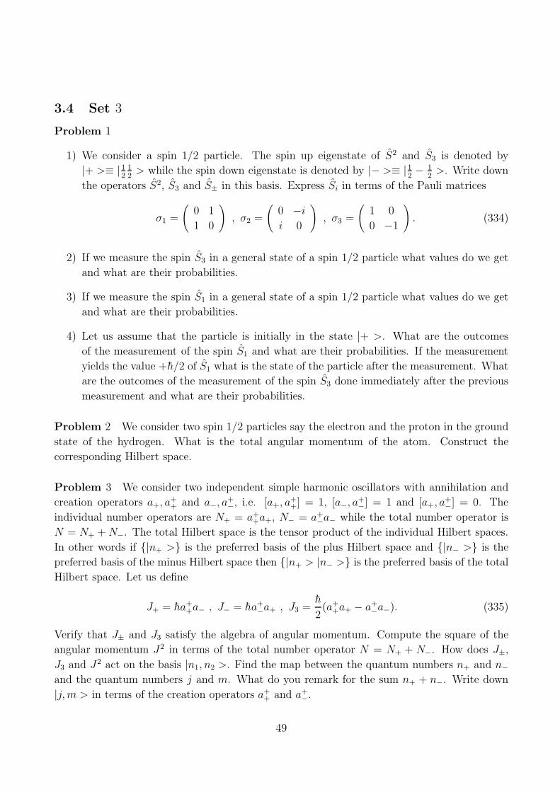
3.4 Set 3
Problem 1
1) We consider a spin 1/2 particle. The spin up eigenstate of S2 and S3 is denoted by
|+ >≡ |12
12> while the spin down eigenstate is denoted by |− >≡ |1
2− 1
2>. Write down
the operators S2, S3 and S± in this basis. Express Si in terms of the Pauli matrices
σ1 =
(
0 1
1 0
)
, σ2 =
(
0 −ii 0
)
, σ3 =
(
1 0
0 −1
)
. (334)
2) If we measure the spin S3 in a general state of a spin 1/2 particle what values do we get
and what are their probabilities.
3) If we measure the spin S1 in a general state of a spin 1/2 particle what values do we get
and what are their probabilities.
4) Let us assume that the particle is initially in the state |+ >. What are the outcomes
of the measurement of the spin S1 and what are their probabilities. If the measurement
yields the value +h/2 of S1 what is the state of the particle after the measurement. What
are the outcomes of the measurement of the spin S3 done immediately after the previous
measurement and what are their probabilities.
Problem 2 We consider two spin 1/2 particles say the electron and the proton in the ground
state of the hydrogen. What is the total angular momentum of the atom. Construct the
corresponding Hilbert space.
Problem 3 We consider two independent simple harmonic oscillators with annihilation and
creation operators a+, a++ and a−, a
+−, i.e. [a+, a
++] = 1, [a−, a
+−] = 1 and [a+, a
+−] = 0. The
individual number operators are N+ = a++a+, N− = a+
−a− while the total number operator is
N = N+ +N−. The total Hilbert space is the tensor product of the individual Hilbert spaces.
In other words if |n+ > is the preferred basis of the plus Hilbert space and |n− > is the
preferred basis of the minus Hilbert space then |n+ > |n− > is the preferred basis of the total
Hilbert space. Let us define
J+ = ha++a− , J− = ha+
−a+ , J3 =h
2(a+
+a+ − a+−a−). (335)
Verify that J± and J3 satisfy the algebra of angular momentum. Compute the square of the
angular momentum J2 in terms of the total number operator N = N+ + N−. How does J±,
J3 and J2 act on the basis |n1, n2 >. Find the map between the quantum numbers n+ and n−and the quantum numbers j and m. What do you remark for the sum n+ + n−. Write down
|j,m > in terms of the creation operators a++ and a+
−.
49
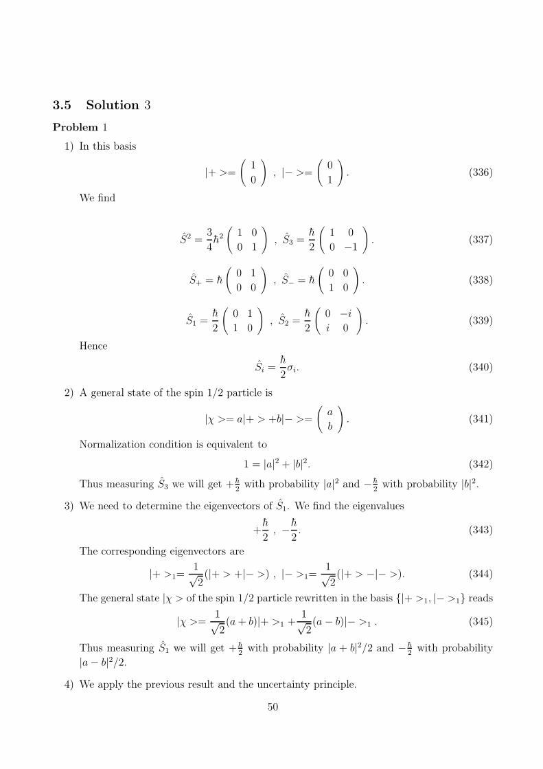
3.5 Solution 3
Problem 1
1) In this basis
|+ >=
(
1
0
)
, |− >=
(
0
1
)
. (336)
We find
S2 =3
4h2
(
1 0
0 1
)
, S3 =h
2
(
1 0
0 −1
)
. (337)
S+ = h
(
0 1
0 0
)
, S− = h
(
0 0
1 0
)
. (338)
S1 =h
2
(
0 1
1 0
)
, S2 =h
2
(
0 −ii 0
)
. (339)
Hence
Si =h
2σi. (340)
2) A general state of the spin 1/2 particle is
|χ >= a|+ > +b|− >=
(
a
b
)
. (341)
Normalization condition is equivalent to
1 = |a|2 + |b|2. (342)
Thus measuring S3 we will get + h2
with probability |a|2 and − h2
with probability |b|2.
3) We need to determine the eigenvectors of S1. We find the eigenvalues
+h
2, − h
2. (343)
The corresponding eigenvectors are
|+ >1=1√2(|+ > +|− >) , |− >1=
1√2(|+ > −|− >). (344)
The general state |χ > of the spin 1/2 particle rewritten in the basis |+ >1, |− >1 reads
|χ >=1√2(a+ b)|+ >1 +
1√2(a− b)|− >1 . (345)
Thus measuring S1 we will get + h2
with probability |a + b|2/2 and − h2
with probability
|a− b|2/2.
4) We apply the previous result and the uncertainty principle.
50
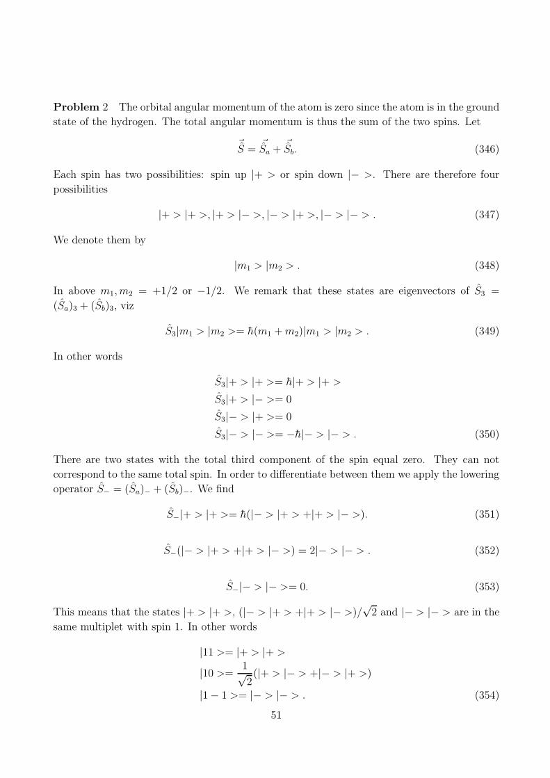
Problem 2 The orbital angular momentum of the atom is zero since the atom is in the ground
state of the hydrogen. The total angular momentum is thus the sum of the two spins. Let
~S =
~Sa +
~Sb. (346)
Each spin has two possibilities: spin up |+ > or spin down |− >. There are therefore four
possibilities
|+ > |+ >, |+ > |− >, |− > |+ >, |− > |− > . (347)
We denote them by
|m1 > |m2 > . (348)
In above m1, m2 = +1/2 or −1/2. We remark that these states are eigenvectors of S3 =
(Sa)3 + (Sb)3, viz
S3|m1 > |m2 >= h(m1 +m2)|m1 > |m2 > . (349)
In other words
S3|+ > |+ >= h|+ > |+ >
S3|+ > |− >= 0
S3|− > |+ >= 0
S3|− > |− >= −h|− > |− > . (350)
There are two states with the total third component of the spin equal zero. They can not
correspond to the same total spin. In order to differentiate between them we apply the lowering
operator S− = (Sa)− + (Sb)−. We find
S−|+ > |+ >= h(|− > |+ > +|+ > |− >). (351)
S−(|− > |+ > +|+ > |− >) = 2|− > |− > . (352)
S−|− > |− >= 0. (353)
This means that the states |+ > |+ >, (|− > |+ > +|+ > |− >)/√
2 and |− > |− > are in the
same multiplet with spin 1. In other words
|11 >= |+ > |+ >
|10 >=1√2(|+ > |− > +|− > |+ >)
|1 − 1 >= |− > |− > . (354)
51
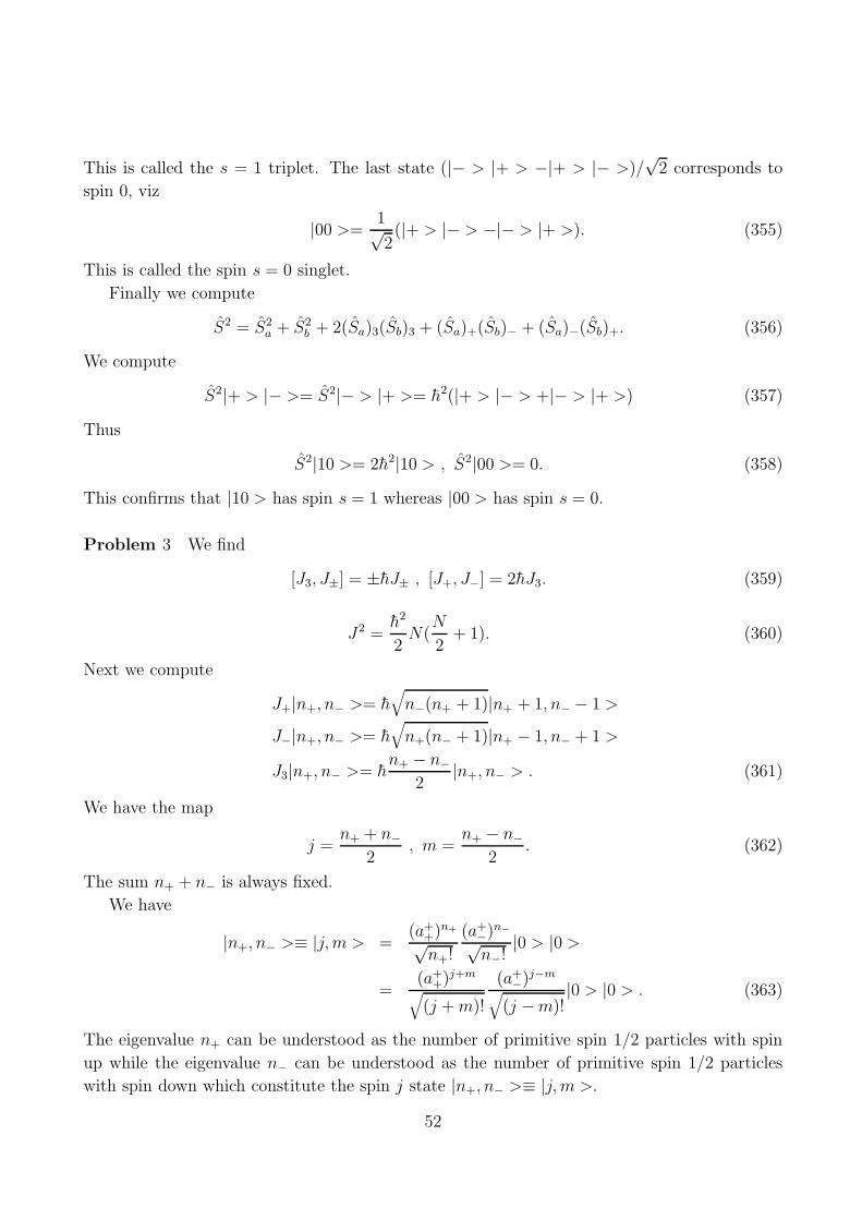
This is called the s = 1 triplet. The last state (|− > |+ > −|+ > |− >)/√
2 corresponds to
spin 0, viz
|00 >=1√2(|+ > |− > −|− > |+ >). (355)
This is called the spin s = 0 singlet.
Finally we compute
S2 = S2a + S2
b + 2(Sa)3(Sb)3 + (Sa)+(Sb)− + (Sa)−(Sb)+. (356)
We compute
S2|+ > |− >= S2|− > |+ >= h2(|+ > |− > +|− > |+ >) (357)
Thus
S2|10 >= 2h2|10 > , S2|00 >= 0. (358)
This confirms that |10 > has spin s = 1 whereas |00 > has spin s = 0.
Problem 3 We find
[J3, J±] = ±hJ± , [J+, J−] = 2hJ3. (359)
J2 =h2
2N(
N
2+ 1). (360)
Next we compute
J+|n+, n− >= h√
n−(n+ + 1)|n+ + 1, n− − 1 >
J−|n+, n− >= h√
n+(n− + 1)|n+ − 1, n− + 1 >
J3|n+, n− >= hn+ − n−
2|n+, n− > . (361)
We have the map
j =n+ + n−
2, m =
n+ − n−2
. (362)
The sum n+ + n− is always fixed.
We have
|n+, n− >≡ |j,m > =(a+
+)n+
√n+!
(a+−)n−
√n−!
|0 > |0 >
=(a+
+)j+m√
(j +m)!
(a+−)j−m
√
(j −m)!|0 > |0 > . (363)
The eigenvalue n+ can be understood as the number of primitive spin 1/2 particles with spin
up while the eigenvalue n− can be understood as the number of primitive spin 1/2 particles
with spin down which constitute the spin j state |n+, n− >≡ |j,m >.
52

4 CHAPTER 4:Perturbation Theory
4.1 Nondegenerate Perturbation Theory
We assume that we can solve exactly for the eigenvalues E0n and the eigenfunctions ψ0
n of
some potential V 0. We call the corresponding Hamiltonian H0. We have
H0|ψ0n >= E0
n|ψ0n > . (364)
< ψ0n|ψ0
m >= δnm. (365)
This is the unperturbed problem.
Now let H be some other Hamiltonian which can be written as
H = H0 + λH1. (366)
The Hamiltonian λH1 is called the perturbation where λ is a small control parameter. The
perturbed problem is defined by
H|ψn >= En|ψn > . (367)
The goal of perturbation theory is to find approximate solutions of this eigenvalue equation in
terms of the exact solutions. In other words we would like to find approximate expressions of
the eigenvalues En and the eigenfunctions ψn in terms of the unperturbed eigenvalues E0n and
the unperturbed eigenfunctions ψ0n.
We write En and ψn in terms of E0n and ψ0
n as
|ψn >= |ψ0n > +λ|ψ1
n > +λ2|ψ2n > +... (368)
En = E0n + λE1
n + λ2E2n + ... (369)
The E1n and |ψ1
n > are the first-order corrections to the nth eigenvalue and eigenfunction
respectively while E2n and |ψ2
n > are the second-order corrections to the nth eigenvalue and
eigenfunction respectively. By substituting (368) and (369) into (367) we find
λ(H0|ψ1n > +H1|ψ0
n >) + λ2(H0|ψ2n > +H1|ψ1
n >) +O(λ3) =
λ(E0n|ψ1
n > +E1n|ψ0
n >) + λ2(E0n|ψ2
n > +E1n|ψ1
n > +E2n|ψ0
n >) +O(λ3). (370)
The first-order perturbation theory is defined by the equation
H0|ψ1n > +H1|ψ0
n > = E0n|ψ1
n > +E1n|ψ0
n > . (371)
Thus
< ψ0n|H0|ψ1
n > + < ψ0n|H1|ψ0
n > = E0n < ψ0
n|ψ1n > +E1
n < ψ0n|ψ0
n > . (372)
53
E1n =< ψ0
n|H1|ψ0n > . (373)
We rewrite (371) as
(H0 −E0n)|ψ1
n > = −(H1 − E1n)|ψ0
n > . (374)
This is an inhomogeneous differential equation for ψ1n. We expand ψ1
n as
|ψ1n >=
∑
m6=nc(n)m |ψ0
m > . (375)
The term involving |ψ0n > is absent since (H0 −E0
n)|ψ0n >= 0. By substitution we obtain
∑
m6=nc(n)m (E0
m − E0n)|ψ0
m > = −(H1 −E1n)|ψ0
n > . (376)
In other words
c(n)m (E0
m −E0n) = − < ψ0
m|H1|ψ0n > . (377)
Equivalently
c(n)m = −< ψ0
m|H1|ψ0n >
E0m − E0
n
. (378)
Hence
|ψ1n > = −
∑
m6=n
< ψ0m|H1|ψ0
n >
E0m − E0
n
|ψ0m > . (379)
The second-order perturbation theory is defined by the equation
H0|ψ2n > +H1|ψ1
n > = E0n|ψ2
n > +E1n|ψ1
n > +E2n|ψ0
n > . (380)
< ψ0n|H0|ψ2
n > + < ψ0n|H1|ψ1
n > = E0n < ψ0
n|ψ2n > +E1
n < ψ0n|ψ1
n > +E2n. (381)
By using the result < ψ0n|ψ1
n >= 0 we obtain
E2n = < ψ0
n|H1|ψ1n >
=∑
m6=n
| < ψ0m|H1|ψ0
n > |2E0n −E0
m
. (382)
We rewrite (380) as
(H0 − E0n)|ψ2
n > = −(H1 − E1n)|ψ1
n > +E2n|ψ0
n > . (383)
This is an inhomogeneous differential equation for ψ2n. We expand ψ2
n as
|ψ2n >=
∑
m6=nd(n)m |ψ0
m > . (384)
54

We calculate
∑
m6=nd(n)m (E0
m −E0n)|ψ0
m > = −(H1 − E1n)|ψ1
n > +E2n|ψ0
n > . (385)
Thus
d(n)k (E0
k −E0n) = − < ψ0
k|(H1 − E1n)|ψ1
n > . (386)
In other words
d(n)k = −< ψ0
k|(H1 −E1n)|ψ1
n >
E0k − E0
n
=∑
m6=n
< ψ0k|H1|ψ0
m >< ψ0m|H1|ψ0
n >
(E0n − E0
k)(E0n −E0
m)− < ψ0
k|H1|ψ0n >< ψ0
n|H1|ψ0n >
(E0n − E0
k)2
. (387)
4.2 Degenerate Perturbation Theory
Let us suppose that there are two unperturbed states |ψ0a > and |ψ0
b > which share the same
unperturbed energy E0. Thus we have
H0|ψ0a >= E0|ψ0
a > , H0|ψ0b >= E0|ψ0
b > , < ψa|ψb >= 0. (388)
Any linear combination of |ψ0a > and |ψ0
b > is also an eigenstate of H0 with the energy E0.
Generally the perturbation λH1 will lift the degeneracy. In other words as we increase λ the
energy level E0 will split into an ”upper” state and a ”lower” state. Equivalently as we decrease
λ the ”upper” state will reduce to one linear combination of |ψ0a > and |ψ0
b > whereas the ”lower”
state will reduce another linear combination of |ψ0a > and |ψ0
b > which is orthogonal to the first.
These are the linear combinations which should be used in (373) in order to calculate the first
order energies. The problem is that these linear combinations are not known to us. We write
these linear combinations in the generic form
|ψ0 >= α|ψ0a > +β|ψ0
b > . (389)
We start from the Schrodinger equation
H|ψ >= E|ψ > . (390)
We expand
E = E0 + λE1 + λ2E2 + ... (391)
|ψ >= |ψ0 > +λ|ψ1 > +λ2|ψ2 > +.... (392)
The first-order perturbation theory is again defined by the equation
H0|ψ1 > +H1|ψ0 > = E0|ψ1 > +E1|ψ0 > . (393)
55
Thus by multiplying both sides of this equation with < ψ0a| we obtain
< ψ0a|H1|ψ0 >= E1 < ψ0
a|ψ0 >
α < ψ0a|H1|ψ0
a > +β < ψ0a|H1|ψ0
b >= E1α. (394)
We define
Wij =< ψ0i |H1|ψ0
j > , i, j = a, b. (395)
We have
αWaa + βWab = αE1. (396)
Similarly by multiplying with < ψ0b | we obtain
αWba + βWbb = βE1. (397)
Multiplying this equation with Wab we get
α|Wab|2 + βWabWbb = βWabE1. (398)
Substituting βWab = αE1 − αWaa we obtain for α 6= 0 the quadratic equation
(E1)2 − (Waa +Wbb)E1 +WaaWbb − |Wab|2 = 0. (399)
The two solutions are
E1± =
1
2
[
Waa +Wbb ±√
(Waa −Wbb)2 + 4|Wab|2]
. (400)
The corresponding linear combinations can then be found by going back to equations (396) and
(397) and solving for α and β.
Let A be a hermitian operator which commutes with H0 and H1. We assume that |ψ0a >
and |ψ0b > are also eigenvectors of A with distinct eigenvalues, viz
A|ψ0a >= µ|ψ0
a > , A|ψ0b >= ν|ψ0
b > , µ 6= ν. (401)
Since [A,H1] = 0 we compute
0 = < ψ0a|[A,H1]|ψ0
b >
= < ψ0a|AH1|ψ0
b > − < ψ0a|H1A|ψ0
b >
= (µ− ν)Wab. (402)
Since µ 6= ν we conclude that Wab = 0. In other words
E1+ = Waa , E
1− = Wbb. (403)
56
This is the result we would obtain using nondegenerate first-order perturbation theory. The
plus sign correspond to α = 1 and β = 0, i.e. |ψ0 >= |ψ0a > whereas the minus sign correspond
to α = 0 and β = 1, i.e. |ψ0 >= |ψ0b >.
In summary if we can find a hermitian operator A which commutes with H we can choose
the common eigenvectors as the unperturbed states and use ordinary first-order perturbation
theory.
Finally in the case of an n-fold degenerate energy level E0 the first-order corrections E1
will be given by the eigenvalues of the n × n matrix Wij =< ψ0i |H1|ψ0
j >. The corresponding
eigenvectors are precisely the good unperturbed states.
4.3 The Fine Structure of Hydrogen
The classical Hamiltonian of the hydrogen atom is
H0 =~p2
2m− e2
4πǫ0
1
r. (404)
The Bohr’s energies are
E0n = − α2
2n2mc2. (405)
The corresponding eigenvectors are |ψ0nlm >. The constant α is known as the fine structure
constant and it is given by
α =e2
4πǫ0hc=
1
137.036. (406)
This is the coupling constant of electromagnetic interactions.
The first correction to En comes from taking into account the motion of the nucleus by
replacing m by the reduced mass mmp/(m + mp). The fine structure of hydrogen consists of
the relativistic correction and of the spin-orbit corrections. It is of order α4mc2. The Lamb
shift is the next correction which is of order α5mc2 and it is due to the quantization of the
electromagnetic field. Next comes the hyperfine structure which is of order (m/mp)α4mc2 and
it is due to the magnetic interaction between the dipole moments of the electron and the proton.
In this section we will only compute the fine structure.
Relativistic Correction The relativistic energy and momentum are given by
E = γmv. (407)
p = γmv. (408)
The factor γ is called the Lorentz factor and it is given by
γ =1
√
1 − v2
c2
. (409)
57
We compute
E2 = p2c2 +m2c4. (410)
The rest energy is
E0 = mc2. (411)
Therefore the kinetic energy is
T = E − E0 =√
p2c2 +m2c4 −mc2
= mc2[
√
1 +p2
m2c2− 1
]
= mc2[
1
2
p2
m2c2− 1
8
p4
m4c4+ ..
]
=p2
2m− p4
8m3c2+ ... (412)
The perturbation is therefore given by the operator
λH1r = − p4
8m3c2. (413)
This perturbation is spherically symmetric and thus it commutes with the square of the angular
momentum L2 and with the third component of the angular momentum L3. The shared eigen-
vectors |ψ0nlm > of H0 (the unperturbed Hamiltonian) and L2 and L3 have distinct eigenvalues
given by h2l(l + 1) and hm for the n2 states which have the same energy En. Thus n, l and m
are good quantum numbers and we can use first-order nondegenerate perturbation theory. The
correction is then given by
λE1r = λ < ψ0
nlm|H1r |ψ0
nlm >
= − 1
8m3c2< ψ0
nlm|p4|ψ0nlm >
= − 1
8m3c2(p2|ψ0
nlm >)+(p2|ψ0nlm >). (414)
In the above equation we have used the fact that p2 is hermitian. The Schrodinger equation
for the unperturbed states reads
p2|ψ0nlm >= 2m(E0
n − V )|ψ0nlm > . (415)
Thus
λE1r = − 1
2mc2< ψ0
nlm|(E0n − V )2|ψ0
nlm >
= − 1
2mc2
[
(E0n)
2 + 2hcαE0n <
1
r> +h2c2α2 <
1
r2>]
. (416)
58
We use the results
<1
r>=
α
n2
mc
h. (417)
<1
r2>=
α2m2c2
h2
1
n3(l + 12). (418)
Substituting these expressions we get
λE1r = −(E0
n)2
2mc2
[
4n
l + 12
− 3]
. (419)
Spin-Orbit Coupling In the electron rest frame the proton circles around the electron and
as a consequence it creates a magnetic field ~B. The current created by the proton is I = e/T
where T is the period of the orbit. The Biot-Savart law tells us that the magnetic field created
by this current is proportional to I and inversely proportional to the radius of the orbit. More
precisely
B =µ0I
2r=µ0e
2rT=
e
2ǫ0rc2T. (420)
This magnetic field is perpendicular to the plane of the orbit. If ~r is the vector from the proton
to the electron and ~v is the velocity of the proton then ~B is in the direction of ~v × ~r. In other
words ~B is in the direction of the orbital angular momentum ~L = m~r × ~v. Thus
~B =e
4πǫ0r3mc2~L. (421)
The electron on the other hand has a spin ~S and as a consequence it has a magnetic dipole mo-
ment ~µ. In fact the magnetic dipole moment is proportional to the spin and the proportionality
factor is called the gyromagnetic ratio.
As an example we calculate the gyromagnetic ratio for a linear charge q distributed uniformly
around a circle of radius r. The circle is rotating about its axis with period T . The magnetic
dipole moment is the current q/T times the area πr2, i.e.
µ =qπr2
T. (422)
The mass of the charge q is equalm and it is also distributed uniformly. The angular momentum
(spin) is equal to the moment of inertia mr2 times the angular frequency 2π/T , viz
S =2πmr2
T. (423)
The corresponding gyromagnetic ratio is therefore
µ
S=
q
2m. (424)
59
The magnetic dipole moment and the spin are in the same direction. Thus
~µ =q
2m~S. (425)
In the case of the electron the magnetic dipole moment is twice this prediction. In other words
~µe = − e
m~S. (426)
The magnetic field created by the motion of the proton will act on the magnetic dipole
moment of the electron in such a way that it will try to align the direction of ~µe along ~B. The
corresponding Hamiltonian is
λH1so = −~µe. ~B
=e2
4πǫ0
1
m2c2r3~S.~L. (427)
The rest frame of the electron is not an inertial frame since it accelerates. The kinematic
correction for this effect consists in multiplying λH1so by a factor of 1/2. This is known as
Thomas precession. We get
λH1so =
e2
8πǫ0
1
m2c2r3~S.~L. (428)
We remark that the correction to the gyromagnetic ratio of the electron and the Thomas
precession cancel exactly one another.
The Hamiltonian λH1so describes the spin-orbit interaction of the hydrogen atom. In quan-
tum mechanics ~S and ~L will be replaced by the operators~S and
~L. The corresponding Hamil-
tonian operator does not commute with~L and
~S. However λH1
so commutes with L2, S2, J2
and J3 where~J is the total angular momentum given by
~J =
~L+
~S. (429)
Since s = 12
the possible eigenvalues of J2 are h2j(j + 1) where
j = l +1
2, j = l − 1
2. (430)
The corresponding eigenvectors are
|jj3 > =∑
m,σ
C lmsσjj3 |lm > |sσ >
= Clj3− 1
2s 1
2
jj3 |lj3 −1
2> |s1
2> +C
lj3+12s 1
2
jj3 |lj3 +1
2> |s− 1
2> . (431)
The coefficients C lmsσjj3 are the Clebsch-Gordon coefficients which satisfy among other things
C lmsσjj3
= 0 unless j3 = m+ σ.
60

The unperturbed eigenvectors will be taken to be the common eigenvectors of H0, L2, S2,
J2 and J3. These are given by
|ψnjj3 >= |Rnl > |jj3 > . (432)
This should be compared with |ψnlm > |sσ >= |Rnl > |lm > |sσ > which are the common
eigenvectors of H0, L2, L3, S2, S3. The unperturbed energies corresponding to either |ψnjj3 >
or |ψnlm > |sσ > are still given by Bohr’ energies.
We compute
S.L =1
2(J2 − S2 − L2). (433)
The eigenvalues corresponding to |ψnjj3 > are
h2
2(j(j + 1) − s(s+ 1) − l(l + 1)) =
h2
2(j(j + 1) − 3
4− l(l + 1)). (434)
The first-order correction is
λE1so = < ψnjj3|λH1
so|ψnjj3 >
=e2
8πǫ0
1
m2c2h2
2(j(j + 1) − 3
4− l(l + 1)) < ψnjj3|
1
r3|ψnjj3 >
=e2
8πǫ0
1
m2c2h2
2(j(j + 1) − 3
4− l(l + 1)) < Rnl|
1
r3|Rnl >
=αh3
4m2c(j(j + 1) − 3
4− l(l + 1)) <
1
r3> . (435)
We use the result
<1
r3>=
α3m3c3
h3n3l(l + 1)(l + 12). (436)
Thus
λE1so =
(E0n)
2
mc2n
l(l + 1)(l + 12)
(
j(j + 1) − 3
4− l(l + 1)
)
. (437)
Explicitly we compute
λE1so =
(E0n)
2
2mc22n
l + 12
1
l + 1, j = l +
1
2. (438)
λE1so = −(E0
n)2
2mc22n
l + 12
1
l, j = l − 1
2. (439)
61
The fine-structure correction is given by
λE1r + λE1
so =(E0
n)2
2mc2(3 − 4n
l + 1) , j = l +
1
2. (440)
λE1r + λE1
so =(E0
n)2
2mc2(3 − 4n
l) , j = l − 1
2. (441)
These two expression can be combined to give
λE1r + λE1
so =(E0
n)2
2mc2(3 − 4n
j + 12
). (442)
The energy levels of hydrogen become
En = E0n + λE1
r + λE1so
= E0n
[
1 +α2
n2(
n
j + 12
− 3
4)]
. (443)
The degeneracy in l is broken. However degeneracy in j is still present.
62

4.4 Set 4
Problem 1
1) We recall the evolution equation of expectation values given by
ihd
dt< Q >=< [Q, H] > . (444)
Use this equation to show that
d
dt< xp >= 2 < T > − < x
∂V
∂x(x) > . (445)
2) Derive the virial theorem
2 < T >=< x∂V
∂x(x) > . (446)
3) For the hydrogen atom show using the virial theorem that
< T >= −< V >
2= −En. (447)
Problem 2
1) Let H be a Hamiltonian which depends on some parameter λ, viz H = H(λ). The
eigenvalues and the eigenvectors will also depend on λ, i.e. En = En(λ) and |ψn >=
|ψn(λ) >. Derive the Feynman-Hellmann theorem given by
∂En∂λ
=< ψn(λ)|∂H∂λ
|ψn(λ) > . (448)
2) The effective Hamiltonian for the radial wave function of the hydrogen is
H = − h2
2m
d2
dr2+
h2
2m
l(l + 1)
r2− e2
4πǫ0
1
r. (449)
The bohr’ energies are
En = − α2mc2
2(jmax + l + 1)2. (450)
Use the Feynman-Hellmann theorem with λ = l to compute the expectation value <
1/r2 >.
63
Problem 3 Show that the radial equation of the hydrogen atom can be put in the form
d2u
dr2=[
l(l + 1)
r2− 2
ar+
1
n2a2
]
u. (451)
The Bohr radius is defined by
a =4πǫ0h
2
me2. (452)
Use the above radial equation to derive Kramer’s relation
s
4[(2l + 1)2 − s2] < rs−2 > −2s + 1
a< rs−1 > +
s+ 1
n2a2< rs >= 0. (453)
Compute the expectation value < r−3 >.
Problem 4 A quantum system can be in three linearly independent states. The Hamiltonian
is given by
Hǫ = V0
1 − ǫ 0 0
0 1 ǫ
0 ǫ 2
, ǫ << 1. (454)
1) Solve the eigenvalue problem of the unperturbed system defined for ǫ = 0.
2) Solve the exact eigenvalue problem defined for any value of ǫ.
3) Use first-order and second-order nondegenerate perturbation theory to find the correction
to the nondegenerate eigenvalue of H0. Compare with the exact result.
4) Use first-order degenerate perturbation theory to find the corrections to the two-fold
degenerate eigenvalue of H0. Compare with the exact result.
Problem 5
1) For the one-dimensional harmonic oscillator the position and momentum operators are
given by
x =
√
h
2mω(a+ + a) , p = i
√
hmω
2(a+ − a). (455)
We also give
a|n >=√n|n− 1 > , a+|n >=
√n+ 1|n+ 1 > . (456)
Compute < n′ |x|n > and < n
′ |x2|n >.
64

2) The three-dimensional harmonic oscillator is given by the potential
V (r) =1
2mω2(x2 + y2 + z2). (457)
Use the method of separation of variables to solve the corresponding Schrodinger equation
and determine the allowed energies. Determine the degeneracy of each energy level.
3) We introduce the perturbation
λH1 = λx2yz. (458)
Use first-order nondegenerate perturbation theory to compute the correction to the ground
state energy.
4) Use first-order degenerate perturbation theory to find the correction to the first excited
energy level.
Problem 6
1) Two nearby polarizable atoms a distance R apart can be modeled by two decoupled
harmonic oscillators which are springs of constant k. We imagine the electrons as point
masses m attached to the springs. The nuclei are heavy and thus they can be supposed
to be motionless sitting at the equilibrium positions of the springs. The displacements of
the two electrons are x1 and x2. The Hamiltonian describing the system is
H0 =1
2mp2
1 +1
2kx2
1 +1
2mp2
2 +1
2kx2
2. (459)
The Coulomb interaction between the two nuclei is e2/R, the Coulomb interaction between
the first nuclei and the second electron is −e2/(R+x2), the Coulomb interaction between
the second nuclei and the first electron is −e2/(R − x1) and the Coulomb interaction
between the two electrons is e2/(R− x1 + x2). The total Coulomb interaction is
H1 =1
4πǫ0
[
e2
R− e2
R− x1− e2
R + x2+
e2
R− x1 − x+ 2
]
. (460)
Show that for |x1| << R and |x2| << R then
H1 = − e2x1x2
2πǫ0R3. (461)
2) We propose the change of variables
x1 =1√2(x+ + x−) , x2 =
1√2(x+ − x−). (462)
p1 =1√2(p+ + p−) , p2 =
1√2(p+ − p−). (463)
Compute the allowed energies of the corresponding quantum system.
65
3) Compute the difference ∆V = E − E0 where E and E0 are the energies of the ground
state with and without the Coulomb interaction.
4) By treating H0 as the unperturbed system and H1 as the perturbation compute the
first-order and second-order corrections of the ground state energy E0. What do you
conclude.
Problem 7 Let ~J be the total angular momentum ~J = ~L + ~S. The eigenvector |jj3 > of
J2, J3, L2 and S2 is given as a linear combination of the eigenvectors |lm > |sσ > of L2, L3,
S2 and S3 with coefficients C lmsσjj3
known as the Clebsch-Gordan coefficients. Compute these
coefficients for s = 12.
Problem 8 The fine structure perturbation is given by the Hamiltonian
H1fs = H1
r +H1so
= − p4
8m3c2+ (
1
2)(−~µs. ~Bint). (464)
The factor of 1/2 in bracket is due to Thomas precession. The magnetic dipole moment as-
sociated with the spin of the electron and the internal magnetic field generated by the orbital
motion are given by
~µs = − e
m~S , ~Bint =
1
4πǫ0
e
mc2r3~L. (465)
We consider another perturbation due to the presence of a non-zero external magnetic field.
The corresponding Hamiltonian is
H1Z = −(~µs + ~µl). ~Bext. (466)
The magnetic dipole moment associated with the angular momentum of the electron is
~µl = − e
2m~L. (467)
This perturbation will lead to Zeeman effect.
1) We consider first the unperturbed problem given by Bohr’s Hamiltonian. Determine
the degree of degeneracy of the energy level n = 2 and write down the corresponding
eigenstates. Express the eigenvectors |lsjj3 > in terms of the eigenvectors |lm > |sσ >using the result of the previous problem.
2) Determine the matrix components < ψnjj3|H1Z|ψnjj3 >.
3) Determine the matrix components < ψnjj3|H1fs|ψnjj3 >.
4) Determine the total perturbation matrix W = H1fs + H1
Z in the eigenstates with n = 2.
Use degenerate perturbation theory to compute the first-order corrections to the energy
level E2.
66
4.5 Solution 4
Problem 1
1) Choose Q = (xp+ px)/2 and use [x, p] = ih and [p, V (x)] = −ih∂V∂x
(x).
2) The expectation values in stationary states are independent of time.
3) First we generalize the virial theorem to 3 dimensions. Then we use ~r.~∇V = r∂V /∂r,
V = −Ke2/r and < H >= En to show that the virial theorem becomes 2 < T >= − <
V >. The expectation values are computed in the states |ψnlm >.
Problem 2
1) We make the expansion
H(λ) = H(0) + λ∂H
∂λ|λ=0 +O(λ2). (468)
The first term will be thought of as the unperturbed Hamiltonian whereas the remaining
terms consist the perturbation. The unperturbed eigenvalue problem is
H(0)|ψn(0) >= En(0)|ψn(0) > . (469)
The first-order correction is therefore
E1n =< ψn(0)|
[
∂H
∂λ|λ=0 +O(λ)
]
|ψn(0) > . (470)
The energy En(λ) is then given by
En(λ) = En(0) + λ < ψn(0)|[
∂H
∂λ|λ=0 +O(λ)
]
|ψn(0) > . (471)
We conclude that
∂En(λ)
∂λ|λ=0 =< ψn(0)|∂H
∂λ|λ=0|ψn(0) > . (472)
2) We compute ∂H/∂l and ∂En/∂l. We find
<1
r2>=
α2m2c2
h2
1
n3(l + 12). (473)
67
Problem 3 The radial equation of the hydrogen atom can be put into the form
d2u
dr2=[
l(l + 1)
r2− 2
ar+
1
n2a2
]
u. (474)
Using this equation we can immediately compute
∫
ursd2u
dr2dr =
∫
urs[
l(l + 1)
r2− 2
ar+
1
n2a2
]
udr
= l(l + 1) < rs−2 > −2
a< rs−1 > +
1
n2a2< rs > . (475)
By integration by parts we get
∫
ursd2u
dr2dr = −
∫
rs(du
dr)2dr − s
∫
urs−1du
drdr
=2
s+ 1
∫
du
dr
d2u
dr2rs+1dr +
s(s− 1)
2< rs−2 > . (476)
We also compute
∫
du
dr
d2u
dr2rs+1dr = − l(l + 1)(s− 1)
2< rs−2 > +
s
a< rs−1 > − s+ 1
2n2a2< rs > . (477)
Putting everything together we get
s
4[(2l + 1)2 − s2] < rs−2 > −2s + 1
a< rs−1 > +
s+ 1
n2a2< rs >= 0. (478)
For s = −1 we get
−1
4[(2l + 1)2 − 1] < r−3 > +
1
a< r−2 >= 0. (479)
Hence
< r−3 >=1
al(l + 1)< r−2 >=
α3m3c3
h3n3l(l + 1)(l + 12). (480)
Problem 4 The solution is straightforward.
Problem 5
1) We find
< n′ |x|n >=
√
h
2mω
(√n + 1δn′ ,n+1 +
√nδn′ ,n−1
)
. (481)
< n′ |x2|n >=
h
2mω
(
√
(n+ 1)(n+ 2)δn′ ,n+2 +√
n(n− 1)δn′ ,n−2 + (2n+ 1)δn′ ,n
)
. (482)
68
2) The Schrodinger equation reads in this case
(
− h2
2m
∂2
∂x2− h2
2m
∂2
∂y2− h2
2m
∂2
∂z2+
1
2mω2(x2 + y2 + z2)
)
Ψ(x, y, z) = EΨ(x, y, z). (483)
Separation of variables yields the allowed energies
En = hω(nx + ny + nz +3
2) , n = nx + ny + nz. (484)
The corresponding states are
Ψ(x, y, z) =< x|nx >< y|ny >< z|nz > . (485)
The degeneracy of the energy level En where n = nx + ny + nz is kept fixed can be
computed as follows. First we fix nx then ny + nz = n− nx. Clearly we have n− nx + 1
possibilities for the pair (ny, nz). Thus the degeneracy of En is given by the formula
d(n) =n∑
nx=0
(n− nx + 1) =n(n+ 1)
2. (486)
3) The first-order correction to the ground state energy E000 = (3hω)/2 which is a nonde-
generate state takes the form
λE1 = < 0| < 0| < 0|λx2yz|0 > |0 > |0 >= λ < 0|x2|0 >< 0|y|0 >< 0|z|0 >= 0. (487)
4) The first excited energy level E1 = (5hω)/2 is three-fold degenerate. The corresponding
states are |100 >, |010 > and |001 >. To compute the first-order correction we need to use
first-order degenerate perturbation theory. More precisely we need to find the eigenvalues
of the perturbation matrix Wij =< i|λH1|j > where i, j = 100, 010, 001. We compute
W =
0 0 0
0 0 ǫ
0 ǫ 0
, ǫ = λ√
2(h
2mω)2. (488)
The eigenvalues are 0, +ǫ and −ǫ with corresponding vectors |100 >, (|010 > +|001 >
)/√
2 and (|010 > −|001 >)/√
2 respectively.
Problem 6
1) Use Taylor expansion.
69
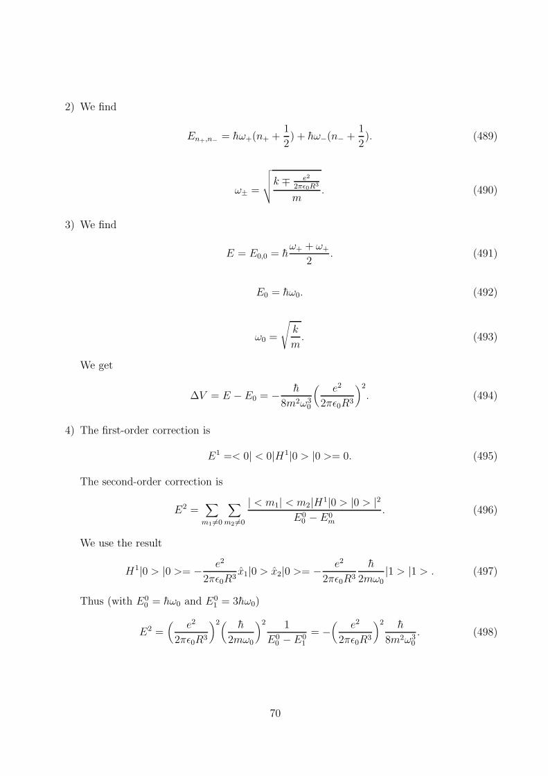
2) We find
En+,n− = hω+(n+ +1
2) + hω−(n− +
1
2). (489)
ω± =
√
√
√
√
k ∓ e2
2πǫ0R3
m. (490)
3) We find
E = E0,0 = hω+ + ω+
2. (491)
E0 = hω0. (492)
ω0 =
√
k
m. (493)
We get
∆V = E − E0 = − h
8m2ω30
(
e2
2πǫ0R3
)2
. (494)
4) The first-order correction is
E1 =< 0| < 0|H1|0 > |0 >= 0. (495)
The second-order correction is
E2 =∑
m1 6=0
∑
m2 6=0
| < m1| < m2|H1|0 > |0 > |2E0
0 − E0m
. (496)
We use the result
H1|0 > |0 >= − e2
2πǫ0R3x1|0 > x2|0 >= − e2
2πǫ0R3
h
2mω0|1 > |1 > . (497)
Thus (with E00 = hω0 and E0
1 = 3hω0)
E2 =(
e2
2πǫ0R3
)2( h
2mω0
)2 1
E00 − E0
1
= −(
e2
2πǫ0R3
)2 h
8m2ω30
. (498)
70
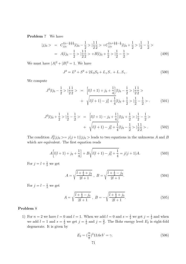
Problem 7 We have
|jj3 > = Clj3− 1
212
12
jj3 |lj3 −1
2> |1
2
1
2> +C
lj3+12
12− 1
2
jj3 |lj3 +1
2> |1
2− 1
2>
= A|lj3 −1
2> |1
2
1
2> +B|lj3 +
1
2> |1
2− 1
2> (499)
We must have |A|2 + |B|2 = 1. We have
J2 = L2 + S2 + 2L3S3 + L+S− + L−S+. (500)
We compute
J2|lj3 −1
2> |1
2
1
2> =
[
l(l + 1) + j3 +1
4
]
|lj3 −1
2> |1
2
1
2>
+
√
l(l + 1) − j23 +
1
4|lj3 +
1
2> |1
2− 1
2> . (501)
J2|lj3 +1
2> |1
2− 1
2> =
[
l(l + 1) − j3 +1
4
]
|lj3 +1
2> |1
2− 1
2>
+
√
l(l + 1) − j23 +
1
4|lj3 −
1
2> |1
2
1
2> . (502)
The condition J23 |jj3 >= j(j+ 1)|jj3 > leads to two equations in the unknowns A and B
which are equivalent. The first equation reads
A[
l(l + 1) + j3 +1
4
]
+B
√
l(l + 1) − j23 +
1
4= j(j + 1)A. (503)
For j = l + 12
we get
A =
√
l + 12
+ j32l + 1
, B =
√
l + 12− j3
2l + 1. (504)
For j = l − 12
we get
A =
√
l + 12− j3
2l + 1, B = −
√
l + 12
+ j32l + 1
. (505)
Problem 8
1) For n = 2 we have l = 0 and l = 1. When we add l = 0 and s = 12
we get j = 12
and when
we add l = 1 and s = 12
we get j = 12
and j = 32. The Bohr energy level E2 is eight-fold
degenerate. It is given by
E2 = (α
8)213.6eV = γ. (506)
71

The eight corresponding states are |ψnjj3 >= |Rnl > |sljj3 > with n = 2, s = 12, l = 0, 1
and j = l + 12, l − 1
2. We will need to express the eigenvectors |sljj3 > in terms of the
eigenvectors |lmsσ >. Using the result of the previous problem we find
|ψ1 >= |01
2
1
2
1
2>= |00 > |1
2
1
2>
|ψ2 >= |01
2
1
2− 1
2>= |00 > |1
2− 1
2> . (507)
|ψ6 >= |11
2
1
2
1
2>=
1√3|10 > |1
2
1
2> −
√
2
3|11 > |1
2− 1
2>
|ψ8 >= |11
2
1
2− 1
2>=
√
2
3|1 − 1 > |1
2
1
2> − 1√
3|10 > |1
2− 1
2> . (508)
|ψ3 >= |11
2
3
2
3
2>= |11 > |1
2
1
2>
|ψ5 >= |11
2
3
2
1
2>=
√
2
3|10 > |1
2
1
2> +
1√3|11 > |1
2− 1
2>
|ψ7 >= |11
2
3
2− 1
2>=
1√3|1 − 1 > |1
2
1
2> +
√
2
3|10 > |1
2− 1
2>
|ψ4 >= |11
2
3
2− 3
2>= |1 − 1 > |1
2− 1
2> . (509)
2) The perturbation due to the external magnetic field is
H1Z = − ~Bext.(~µl + ~µs)
=e
2mBext(L3 + 2S3)
=µBBext
h(L3 + 2S3)
=β
h(L3 + 2S3). (510)
In the above equations the magnetic field was taken along the third direction and µB and
β are defined by
µB =eh
2m, β = µBBext. (511)
We compute
(L3 + 2S3)|ψ1 >= h|ψ1 >
(L3 + 2S3)|ψ2 >= −h|ψ2 >
(L3 + 2S3)|ψ3 >= 2h|ψ3 >
72
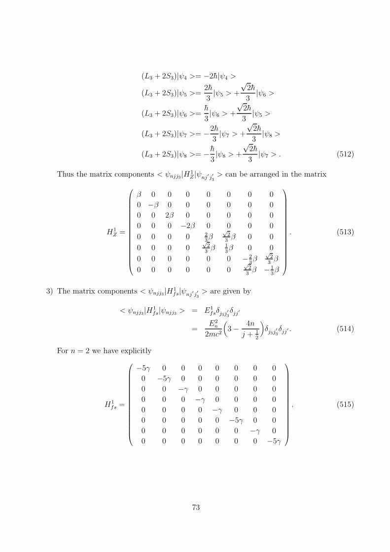
(L3 + 2S3)|ψ4 >= −2h|ψ4 >
(L3 + 2S3)|ψ5 >=2h
3|ψ5 > +
√2h
3|ψ6 >
(L3 + 2S3)|ψ6 >=h
3|ψ6 > +
√2h
3|ψ5 >
(L3 + 2S3)|ψ7 >= −2h
3|ψ7 > +
√2h
3|ψ8 >
(L3 + 2S3)|ψ8 >= − h3|ψ8 > +
√2h
3|ψ7 > . (512)
Thus the matrix components < ψnjj3|H1Z|ψnj′j′3 > can be arranged in the matrix
H1Z =
β 0 0 0 0 0 0 0
0 −β 0 0 0 0 0 0
0 0 2β 0 0 0 0 0
0 0 0 −2β 0 0 0 0
0 0 0 0 23β
√2
3β 0 0
0 0 0 0√
23β 1
3β 0 0
0 0 0 0 0 0 −23β
√2
3β
0 0 0 0 0 0√
23β −1
3β
. (513)
3) The matrix components < ψnjj3|H1fs|ψnj′j′3 > are given by
< ψnjj3|H1fs|ψnjj3 > = E1
fsδj3j′3δjj′
=E2n
2mc2
(
3 − 4n
j + 12
)
δj3j′3δjj′ . (514)
For n = 2 we have explicitly
H1fs =
−5γ 0 0 0 0 0 0 0
0 −5γ 0 0 0 0 0 0
0 0 −γ 0 0 0 0 0
0 0 0 −γ 0 0 0 0
0 0 0 0 −γ 0 0 0
0 0 0 0 0 −5γ 0 0
0 0 0 0 0 0 −γ 0
0 0 0 0 0 0 0 −5γ
. (515)
73
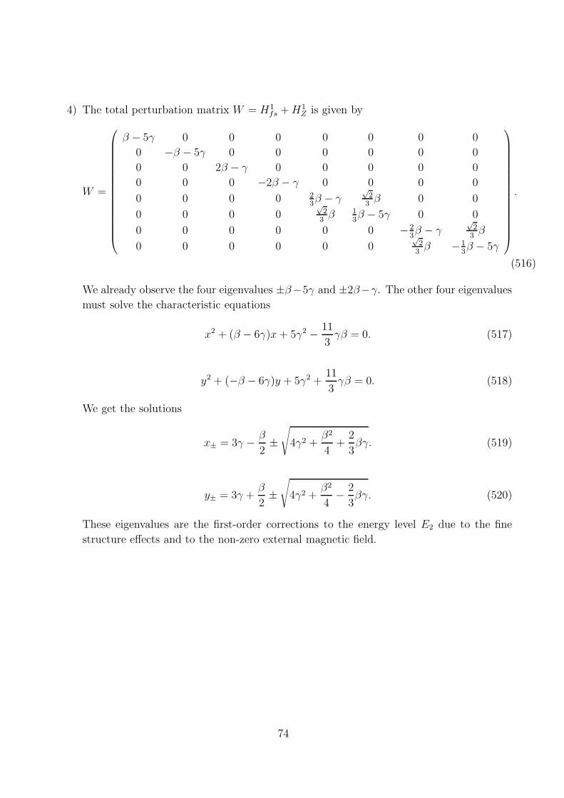
4) The total perturbation matrix W = H1fs +H1
Z is given by
W =
β − 5γ 0 0 0 0 0 0 0
0 −β − 5γ 0 0 0 0 0 0
0 0 2β − γ 0 0 0 0 0
0 0 0 −2β − γ 0 0 0 0
0 0 0 0 23β − γ
√2
3β 0 0
0 0 0 0√
23β 1
3β − 5γ 0 0
0 0 0 0 0 0 −23β − γ
√2
3β
0 0 0 0 0 0√
23β −1
3β − 5γ
.
(516)
We already observe the four eigenvalues ±β−5γ and ±2β−γ. The other four eigenvalues
must solve the characteristic equations
x2 + (β − 6γ)x+ 5γ2 − 11
3γβ = 0. (517)
y2 + (−β − 6γ)y + 5γ2 +11
3γβ = 0. (518)
We get the solutions
x± = 3γ − β
2±√
4γ2 +β2
4+
2
3βγ. (519)
y± = 3γ +β
2±√
4γ2 +β2
4− 2
3βγ. (520)
These eigenvalues are the first-order corrections to the energy level E2 due to the fine
structure effects and to the non-zero external magnetic field.
74
5 CHAPTER 5: Scattering Theory
5.1 Classical Scattering Theory
5.1.1 The 2−Body Central Force Problem
Let ~r1 and ~r2 be the position vectors of two mass points m1 and m2 interacting through a
force due to the potential energy U = U(~r, ~r) where ~r is the relative position vector defined
by ~r = ~r2 − ~r1. It is not difficult to argue that the central force motion of these two bodies
about their center of mass can be reduced to the motion about the center of mass of a single
body which is the reduced mass. The center of mass is found at the point with position vector~R = (m1~r1 +m2~r2)/(m1 +m2) and the reduced mass is defined by µ = m1m2/(m1 +m2). This
fact follows from the identity
1
2(m1~r1
2+m2~r2
2) =
m1 +m2
2~R +
1
2µ~r
2. (521)
We consider therefore a single particle of massmmoving under the influence of a conservative
force, i.e. ~F = −~∇V where the potential V depends only on the radial distance r from the
origin. This is a central force problem where the force on the particle is along ~r. This problem
is clearly spherically symmetric. Thus the angular momentum ~L = ~r × ~p must be conserved
which can be checked explicitly by computing the time derivative d~L/dt. This means that ~r is
perpendicular to the direction of ~L which is fixed. In other words central force motion happens
in a plane. The kinetic energy will then read
T =1
2m~r
2=
1
2m(r2 + r2θ2). (522)
The Lagrangian is
L =1
2m(r2 + r2θ2) − V (r). (523)
The first Lagrange equation is
∂L
∂θ− d
dt
∂L
∂θ= 0 ⇔ d
dt(mr2θ) = 0. (524)
In other words
mr2θ = l. (525)
The number l is the magnitude of the angular momentum. It is not difficult to see that r2θ/2
is the areal velocity, i.e. the area swept out by the vector ~r in one second. Hence conservation
of angular momentum is equivalent to Kepler’s second law which states that the radius vector
~r sweeps out equal area in equal times.
The second Lagrange equation is
∂L
∂r− d
dt
∂L
∂r= 0 ⇔ mr −mrθ2 = −∂V
∂r= f(r). (526)
75
Since the force is conservative the total energy must be conserved. This can be shown as follows.
First we write the above equation of motion as
mr = mrθ2 − ∂V
∂r
=l2
mr3− dV
dr
= − d
dr(1
2
l2
mr2+ V ). (527)
Multiplying by r we get
mrr = −drdt
d
dr(1
2
l2
mr2+ V ). (528)
Equivalently
d
dt
(
1
2mr2 +
1
2
l2
mr2+ V
)
= 0. (529)
The quantity in bracket is precisely the total energy of the system and it is clearly conserved.
We write
E =1
2mr2 +
1
2
l2
mr2+ V. (530)
Solving for r we get
r =
√
2
m
(
E − V − l2
2mr2). (531)
Thus
dt =dr
√
2m
(
E − V − l2
2mr2)
. (532)
Integrating both sides from t = 0 where r(0) = r0 to t where r(t) = r we get
t =∫ r
r0
dr√
2m
(
E − V − l2
2mr2)
. (533)
This gives t = t(r). Inverting we get r = r(t). The angle θ can then be obtained from
dθ =ldt
mr2(t). (534)
Integrating from t = 0 where θ(0) = θ0 to t where θ(t) = θ we get
θ =∫ t
0
ldt
mr2(t)+ θ0. (535)
76
The equation of the orbit r = r(θ) can be found as follows. From the equation of motion (525)
we have
mr2dθ = ldt. (536)
By putting this equation in (532) we get
dθ =ldr
mr2
√
2m
(
E − V − l2
2mr2)
. (537)
Integrating from r0 where θ(r0) = θ0 to r where θ(r) = θ we get
θ =∫ r
r0
ldr
mr2
√
2m
(
E − V − l2
2mr2)
+ θ0
=∫ r
r0
dr
r2√
2m(E−V )l2
− 1r2
+ θ0. (538)
We consider now the inverse square law
V = −kr, f = − k
r2. (539)
We also consider the indefinite integral (with u = 1/r)
θ =∫
dr
r2√
2m(E−V )l2
− 1r2
= −∫ du√
2mEl2
+ 2mkul2
− u2. (540)
We use the formula
∫ dx√α + βx+ γx2
=1√−γ arccos−β + 2γx
√q
, q = β2 − 4αγ. (541)
Hence we obtain (including a constant of integration θ′)
θ = − arccosl2umk
− 1√
1 + 2l2Emk2
+ θ′
. (542)
Thus we get
1
r= C(1 + e cos(θ − θ
′
)) , C =mk
l2, e =
√
1 +2El2
mk2. (543)
77

The orbit is therefore a conic section with one focus at the origin where e is the eccentricity.
The nature of the orbit is as follows
e > 1 ⇔ E > 0 : hyperbola
e = 1 ⇔ E = 0 : parabola
e < 1 ⇔ E < 0 : ellipse
e = 0 ⇔ E = −mk2
2l2: circle. (544)
5.1.2 Differential Cross-Section
We imagine a uniform beam of particles with the same mass and energy incident upon
a center of force. The force is assumed to vanish at infinity. In other words the orbit of
the incoming particles when they are far from the center of force is a straight line trajectory.
The orbit will deviate from the incident straight line trajectory when the particles come near
the center of force and after passing the center of force the orbit will eventually become a
straight line trajectory once again. The scattering angle Θ is the angle between the straight
line trajectory of incoming particles and the straight line trajectory of outgoing particles.
The periapsis is the axis which goes through the center of force and through the point of
closest approach which is a distance rm from the center of force. Let Ψ be the angle between
the straight line trajectory of incoming particles and the periapsis. Since the orbit is symmetric
about the direction of the periapsis one must have
Θ = π − 2Ψ. (545)
The perpendicular distance b between the direction of the incident beame of particles and the
center of force is called the impact parameter. In some sense the impact parameter replaces
the angular momentum l of the incident particles. Indeed we compute
l = mv0b = b√
2mE. (546)
Clearly incoming particles which are incident within an infinitesimal cross-sectional area dσ will
scatter into a solid angle dΩ. The proportionality factor is called the differential cross-section
which is defined by
D(Ω) =dσ
dΩ. (547)
The physical meaning of D(Ω) is as follows. Let I be the intensity (luminosity) of the incident
beam, i.e. the number of incident particles per unit area normal to the beam per unit time.
The number of particles which cross dσ per unit time is therefore dN = Idσ = ID(Ω)dΩ. In
other words
D(Ω) =1
I
dN
dΩ. (548)
78
This means that ID(Ω)dΩ is the number of particles scattered into the solid angle dΩ per unit
time. This must be a positive quantity. For central potentials there is a full symmetry around
the axis of the incident beam. Thus we can write dσ = 2πbdb and dΩ = 2π sin ΘdΘ. We obtain
then the differential cross-section
D(Θ) =b
sin Θ| dbdΘ
|. (549)
Since Θ decreases as b increases the derivative db/dΘ is negative and thus the introduction of
the absolute signs in order to maintain the positivity of D(Θ). The total cross-section is given
by
σ =∫
D(Θ)dΩ. (550)
5.1.3 Rutherford Scattering
As an example of the scattering of particles by a center of force we consider the case of a
repulsive Coulomb force between a fixed charge q1 = −Ze and a charge q2 = −Z ′e. Then
k = − q1q24πǫ0
. (551)
For a scattering problem the energy E is positive and thus e > 1. By choosing θ′= π in (673)
the periapsis will correspond to θ = 0 since this gives the smallest value of r. The orbit becomes
1
r=mq1q24πǫ0l2
(e cos θ − 1). (552)
The eccentricity is given by
e =
√
1 +(
8πǫ0Eb
q1q2
)2
. (553)
The direction of incoming particles corresponds to θ = Ψ when r −→ ∞. In other words
cos Ψ =1
e. (554)
Equivalently
sinΘ
2=
1
e⇔ cot
Θ
2=
√e2 − 1 =
8πǫ0Eb
q1q2. (555)
In other words
b =q1q2
8πǫ0Ecot
Θ
2. (556)
The differential cross-section is
D(Ω) =1
4
(
q1q28πǫ0E
)2 1
sin4 Θ2
. (557)
The total cross-section σ =∫
dΩD(Ω) is then obviously infinite. This is due to the fact that
the range of the Coulomb interaction is infinite.
79
5.2 Quantum Scattering Theory
5.2.1 Lippmann-Schwinger Equation
We consider the time-independent Schrodinger equation
(H0 + V )|ψ >= E|ψ > . (558)
The Hamiltonian H0 is the kinetic energy operator, viz
H0 =~p2
2m. (559)
The spectra of H0 and H0 + V are assumed to be continuous. Let |φ > be the eigenvector of
H0 with energy E, i.e.
H0|φ >= E|φ > . (560)
The goal is to find a solution |ψ > to (558) with the same energy E such that as V −→ 0 we
have |ψ >−→ |φ >. This corresponds to elastic scattering where there is no change in energy.
The Schrodinger equation (558) can be put in the form
(E −H0)|ψ >= (E −H0)|φ > +V |ψ > . (561)
Thus we have the formal solution
|ψ >= |φ > +1
E −H0
V |ψ > . (562)
In order to get a meaningful solution we use Feynman prescription. We make E slightly complex.
We get
|ψ± >= |φ > +1
E −H0 ± iǫV |ψ± > . (563)
This is the Lippmann-Schwinger equation. In the position basis we have
< ~x|ψ± > = < ~x|φ > + < ~x| 1
E −H0 ± iǫV |ψ± >
= < ~x|φ > +∫
d3x′
< ~x| 1
E −H0 ± iǫ|~x′
>< ~x′ |V |ψ± > . (564)
Thus we must evaluate the kernel of this integral given by
G±(~x, ~x′
) =h2
2m< ~x| 1
E −H0 ± iǫ|~x′
>
=h2
2m
∫
d3~p′∫
d3~p′′
< ~x|~p′
>< ~p′| 1
E −H0 ± iǫ|~p′′
>< ~p′′ |~x′
> . (565)
80
We use the results
< ~x|~p′
>=e
ih~p′~x
(2πh)32
, < ~p′′ |~x′
>=e−
ih~p′′~x′
(2πh)32
. (566)
< ~p′ | 1
E −H0 ± iǫ|~p′′
>=δ3(~p
′ − ~p′′)
E − ~p′2
2m± iǫ
. (567)
Thus (with E = h2k2/(2m), ~p′= h~q and ~R = ~x− ~x
′)
G±(~x, ~x′
) =h2
2m
∫
d3~p′
(2πh)3
eih~p′(~x−~x′)
E − ~p′2
2m± iǫ
=∫
d3~q
(2π)3
ei~q~R
k2 − q2 ± iǫ. (568)
From this equation it is obvious that G±(~x, ~x′) solves the Helmholtz equation with a delta
function source, viz
(~∇2 + k2)G±(~x, ~x′
) = δ3(~x− ~x′
). (569)
The function G±(~x, ~x′) is the Green’s function for the Helmholtz equation. It measures the
response to a delta function source.
The vector ~R is fixed. We can choose the z axis along ~R. Thus we get
G±(~x, ~x′
) =∫
q2 sin θdqdθdφ
(2π)3
eiqR cos θ
k2 − q2 ± iǫ
=i
8π2R
∫ ∞
−∞
[
qe−iqRdq
k2 − q2 ± iǫ− qeiqRdq
k2 − q2 ± iǫ
]
=i
8π2R(−I2 + I1). (570)
I1 =∫ ∞
−∞
qeiqRdq
−k2 + q2 ∓ iǫ. (571)
I2 =∫ ∞
−∞
qe−iqRdq
−k2 + q2 ∓ iǫ. (572)
The poles are given by the condition q2± = k2 ± iǫ. For G+ the poles are at q± = ±(k + iǫ
′)
whereas for G− the poles are at q± = ±(k − iǫ′).
We will evaluate these two integrals using Cauchy’s integral formula given by
∮
f(z)dz
z − z0= 2πif(z0). (573)
81
Thus we need to close the contour of integration without changing the values of the integrals.
The exponential factor eiqR which appears in I1 will approach zero if q is on a semicircle of
infinite radius in the upper half of the complex plane. Hence we close the contour of integration
of I1 by adding a semicircle at infinity in the upper half of the complex plane. For G+ it is the
pole (k + iǫ′) which lies within the contour whereas for G− it is the pole −(k − iǫ
′) which lies
within the contour. Thus we obtain (with f(z) = zeizR/(z + z0) and z0 = ±(k ± iǫ′))
I1 = 2πif(z0) = 2πi(1
2eiz0R) = πie±ikR. (574)
Similarly we close the contour of integration of I2 by adding a semicircle at infinity in the
lower half of the complex plane. For G+ it is the pole −(k + iǫ′) which lies within the contour
whereas for G− it is the pole (k − iǫ′) which lies within the contour. Thus we obtain (with
f(z) = ze−izR/(z + z0) and z0 = ∓(k ± iǫ′))
I2 = −2πif(z0) = −2πi(1
2e−iz0R) = −πie±ikR. (575)
The minus sign is due to the fact that we are going in the clockwise direction. We get finally
the Green’s function
G±(~x, ~x′
) = − 1
4π
e±ikR
R. (576)
The Lippmann-Schwinger equation in position basis becomes
< ~x|ψ± > = < ~x|φ > −2m
h2
1
4π
∫
d3x′ e±ik|~x−~x
′ |
|~x− ~x′| < ~x′ |V |ψ± > . (577)
For local potentials we have < ~x′|V |ψ± >= V (~x
′) < ~x
′ |ψ± > and hence
< ~x|ψ± > = < ~x|φ > − m
2πh2
∫
d3x′ e±ik|~x−~x
′ |
|~x− ~x′ | V (~x′
) < ~x′ |ψ± > . (578)
The vector ~x defines the observation point P where a detector is placed. For a finite range
potential only a small region of space will give a nonzero contribution to the integral over
~x′. In scattering problems the observation point P is typically far outside the range of the
potential because we can not place the detector near the scattering center. Hence one must
have |~x| >> |~x′ |. Therefore (with |~x| = r, |~x′| = r′, r = ~x/|~x| and α is the angle between ~x and
~x′)
|~x− ~x′ | =
√
r2 + r′2 − 2rr′ cosα
= r
√
1 +r′2
r2− 2
~x′ r
r
= r − ~x′
r +O(1
r). (579)
82
Thus
e±ik|~x−~x′ |
|~x− ~x′ | ≃ e±ikre∓i~k′~x′
r, ~k
′
= kr. (580)
The vector h~k′is the momentum of the scattered particles reaching the observation point P .
The momentum of the incident particles is ~pi = h~k and the corresponding state vector is
|φ >= |~k >. We must therefore have
< ~x|φ >=< ~x|~k >=ei~k~x
(2π)32
. (581)
Hence for large distances r the Lippmann-Schwinger equation becomes
< ~x|ψ± >=1
(2π)32
[
ei~k~x +
e±ikr
rf(~k
′
, ~k)]
. (582)
f(~k′
, ~k) = −m
h2
√2π∫
d3x′
e∓i~k′~x′
V (~x′
) < ~x′ |ψ± > . (583)
Thus the spatial dependence of the positive (negative) solution at large r is given by the sum
of the incident plane wave and the outgoing (incoming) spherical wave which is caused by the
scattering center. In most scattering experiments it is the positive solution that is realizable.
In the remaining discussion we will only consider the positive solution.
Let v0 be the velocity of the incident beam. The probability that a particle crosses an
infinitesimal area dσ normal to the direction of the incident beam in a time interval dt is
dPincident = |A|2(v0dtdσ). (584)
This probability must be equal to the probability dPscattered that a particle scatteres into the
solid angle dΩ in a times interval dt. In other words dPscattered is the probability that a particle
crosses the surface r2dΩ in a time interval dt, viz
dPincident =|A|2|f |2r2
(v0dt r2dΩ). (585)
Hence the differential cross-section is given by
D(Ω) =dσ
dΩ= |f(~k
′
, ~k)|2. (586)
The coefficient f(~k′, ~k) which is called the scattering amplitude is the probability amplitude of
scattering in the direction Θ which is the angle between ~k and ~k′.
83
5.2.2 The Born Approximation
We write the Lippmann-Schwinger equation and the scattering amplitude as
< ~x|ψ+ >=1
(2π)32
[
ei~k~x +
e+ikr
rf(kr,~k)
]
. (587)
f(kr,~k) = −m
h2
√2π∫
d3x′
e−ikr~x′
V (~x′
) < ~x′ |ψ+ > . (588)
By using the Lippmann-Schwinger equation we can rewrite the scattering amplitude as
f(kr,~k) = −m
h2
√2π∫
d3x′
e−ikr~x′
V (~x′
)1
(2π)32
(
ei~k~x
′
+e+ikr
′
r′ f(kr′
, ~k))
. (589)
The first Born approximation consists in droppening the second term in parantheses, viz
f (1)(kr,~k) = −m
h2
√2π∫
d3x′
e−ikr~x′
V (~x′
)1
(2π)32
ei~k~x
′
= − m
2πh2
∫
d3x′
ei(~k−kr)~x′V (~x
′
). (590)
This is essentially the Fourier transform of the potential. The momentum transfer in the process
is given by h~q where ~q = ~k − kr. In terms of the scattering angle Θ we compute
q = 2k sinΘ
2. (591)
We choose the axis z along the direction of ~q. Then
f (1)(kr,~k) = − m
2πh2
∫
r′2 sin θdr
′
dθdφeiqr′cos θV (~x
′
). (592)
For a spherically symmetric potential V (~x′) = V (r
′) we have
f (1)(kr,~k) =m
h2
∫
r′2dr
′
d cos θeiqr′cos θV (r
′
)
= −2m
qh2
∫
r sin qrV (r)dr. (593)
To see the nature of higher-order Born corrections we go back to Lippmann-Schwinger equation
in the form (683). We introduce the notation ψ+(~x) =< ~x|ψ+ >, φ(~x) =< ~x|φ > and
G(~x− ~x′
) = − m
2πh2
e+ik|~x−~x′ |
|~x− ~x′ | . (594)
The Lippmann-Schwinger equation becomes
ψ+(~x) = φ(~x) +∫
G(~x− ~x1)V (~x1)ψ+(~x1)d
3x1. (595)
84
We can immediately get the series
ψ+(~x) = φ(~x) +∫
G(~x− ~x1)V (~x1)φ(~x1)d3x1 +
∫ ∫
G(~x− ~x1)V (~x1)G(~x1 − ~x2)V (~x2)φ(~x2)d3x1d
3x2
+∫ ∫ ∫
G(~x− ~x1)V (~x1)G(~x1 − ~x2)V (~x2)G(~x2 − ~x3)V (~x3)φ(~x3)d3x1d
3x2d3x3 + ... (596)
This is known as the Born series. In the nth term the incident wave function φ interacts n times
with the potential before it propagates to infinity via the Green’s function G. Each interaction
is expressed in terms of a vertex factor equal to the potential and between two successive
interactions the wave function propagates via the Green’s function G. The Green’s function G
is therefore also known as the propagator. The Born series can thus be understood as vertex
factors V and propagators G connected to form diagrams known as Feynman diagrams.
5.2.3 Transition Operator
The scattering amplitude is
f(kr,~k) = −m
h2
√2π∫
d3x′
e−ikr~x′
V (~x′
) < ~x′ |ψ+ >
= −m
h2 (2π)2 < kr|V |ψ+ > . (597)
We define the transition operator T by
V |ψ+ >= T |φ > , |φ >= |~k > . (598)
Hence
f(kr,~k) = −m
h2
√2π∫
d3x′
e−ikr~x′
V (~x′
) < ~x′ |ψ+ >
= −m
h2 (2π)2 < kr|T |~k > . (599)
Multiplying the Lippmann-Schwinger equation by V we get
V |ψ+ > = V |φ > +V1
E −H0 + iǫV |ψ+ > . (600)
In other words
T |φ > = V |φ > +V1
E −H0 + iǫT |φ > . (601)
Since the momentum eigenvectors |φ >= |~k > are complete we obtain
T = V + V1
E −H0 + iǫT
= V + V1
E −H0 + iǫV + V
1
E −H0 + iǫV
1
E −H0 + iǫV + ... (602)
85
5.3 Method of Phase Shifts
5.3.1 Schrodinger Equation in the Region V = 0
We consider Schrodinger equation for a central potential V (r) which is of finite range. The
wave functions are of the form
ψ(r, θ, φ) = R(r)Y ml (θ, φ). (603)
The radial equation for u = rR reads
− h2
2m
d2u
dr2+[
V (r) +h2
2m
l(l + 1)
r2
]
u = Eu. (604)
For very large r in the radiation zone where we can neglect both the central potential and the
centrifugal potential we get
d2u
dr2= −k2u , k2 =
2mE
h2 . (605)
Thus
u = Aeikr +Be−ikr. (606)
For a scattered wave we must have B = 0. Hence we get
R = Aeikr
r. (607)
In the Intermediate zone where we can only neglect the central potential we have
d2u
dr2− l(l + 1)
r2= −k2u. (608)
The general solution is a linear combination of spherical Bessel functions, viz
R = Ajl(kr) +Bnl(kr). (609)
The spherical Bessel functions of order l are generalization of the sine function. They are
defined by
jl(x) = (−x)l( 1
x
d
dx)l
sin x
x−→ 2ll!
(2l + 1)!xl , x −→ 0. (610)
The spherical Neumann functions of order l are generalization of the cosine function. They are
also known as Bessel functions of the second kind. They are defined by
nl(x) = −(−x)l( 1
x
d
dx)l
cosx
x−→ −(2l)!
2ll!
1
xl+1, x −→ 0. (611)
86
The generalizations of the exponential functions e±ix are the so-called Hankel functions. The
spherical Hankel functions are defined by
h(1)l (x) = jl(x) + inl(x) −→
(−i)l+1
xeix , x −→ ∞. (612)
h(2)l (x) = jl(x) − inl(x) −→
(i)l+1
xe−ix , x −→ ∞. (613)
The general solution R can therefore be written as a linear combination of spherical Hankel
functions, viz
R = Ch(1)l (kr) +Dh
(2)l (kr). (614)
From the behavior at large r we see that h(1)l corresponds to an outgoing spherical wave whereas
h(2)l corresponds to an incoming spherical wave. In other words for scattered wave we need
D = 0. We obtain
R = Ch(1)l (kr). (615)
The wave function outside the scattering region where V = 0 is of the form
ψ(r, θ, φ) = A[
eikz +∑
l,m
Clmh(1)l (kr)Y m
l (θ, φ)]
. (616)
The z axis is chosen along the direction of the incident beam. A central potential is spherically
symmetric and thus the wave function can not depend on φ. In other words only the terms
with m = 0 contribute. Recall
Y 0l (θ, φ) =
√
2l + 1
4πPl(cos θ). (617)
We introduce the lth partial wave amplitude al by the equation Cl0 = il+1k√
4π(2l + 1)al. We
get
ψ(r, θ) = A[
eikz + k∑
l
il+1(2l + 1)alh(1)l (kr)Pl(cos θ)
]
. (618)
For large r we get
ψ(r, θ) −→ A[
eikz + f(θ)eikr
r
]
, r −→ ∞. (619)
The scattering amplitude is given in terms of the partial wave amplitudes by
f(θ) =∑
l
(2l + 1)alPl(cos θ). (620)
87
It remains to determine the partial wave amplitudes by solving the Schrodinger equation in the
scattering region where V 6= 0.
From the above discussion it is clear that the incident plane wave eikz since it solves the
Schrodinger equation with V = 0 it can be written in terms of spherical Bessel functions and
spherical harmonics. The expansion will read
eikz =∑
lm
(
Almjl(kr) +Blmnl(kr))
Y ml (θ, φ). (621)
The Neumann functions blow up at the origin and thus we must have Blm = 0. Furthermore
since z = r cos θ only the terms with m = 0 will contribute. Hence we get
eikz =∑
l
ilCl(2l + 1)jl(kr)Pl(cos θ). (622)
An integral representation of the Bessel function is given by
jl(q) =1
2il
∫ +1
−1eiqxPl(x)dx. (623)
We can use this identity to show that Cl = 1 and hence
eikz =∑
l
il(2l + 1)jl(kr)Pl(cos θ). (624)
This is called Rayleigh’s formula.
5.3.2 Plane and Spherical Waves
The eigenvectors of the Hamiltonian H0 of a free particle can be taken to be the plane-wave
state vectors |~k > which satisfy the orthonormalization condition
< ~k′ |~k >= δ3(~k − ~k
′
). (625)
The Hamiltonian H0 commutes with the angular momentum operators L2 and L3. Thus the
eigenvectors of H0 can also be taken to be the simultaneous eigenvectors of H0 ,L2 and L3
which we denote |Elm >. These are precisely the spherical-wave state vectors which satisfy
the orthonormalization condition
< E′
l′
m′ |Elm >= δll′δmm′ δ(E −E
′
). (626)
It is clear that the momentum space spherical wave function < ~k|Elm > is proportional to
δ(E − h2k2
2m). We write
< ~k|Elm >=h√mk
δ(E − h2k2
2m)Xm
l (k, k). (627)
88

We compute∫
d3~k < E′
l′
m′ |~k >< ~k|Elm >= δ(E − E
′
)∫
dΩXm′
l′ (k, k)(Xml (k, k))∗. (628)
In the above equation dΩ is the solid angle which corresponds to the unit vector k and k is
fixed such that k =√
2mE/h2. We must have∫
dΩXm′
l′ (k, k)(Xml (k, k))∗ = δl′ lδm′m. (629)
The solution is immediately given by the spherical harmonics, viz
Xml (k, k) = Xm
l (k) = Y ml (k). (630)
The plane-wave state vector |~k > can be expanded in terms of the spherical-wave state vectors
|Elm > as
|~k > =∑
l
∑
m
∫
dE|Elm >< Elm|~k >
=h√mk
∑
l
∑
m
|Elm > (Y ml (k))∗ , E =
h2k2
2m. (631)
We need to compute now
< ~x|~k > =h√mk
∑
l
∑
m
< ~x|Elm > (Y ml (k))∗ , E =
h2k2
2m. (632)
The position space spherical wave function is < ~x|Elm >. From the previous section it is clear
that the spherical waves are given by
< ~x|Elm >= cljl(kr)Yml (r). (633)
Thus
ei~k~x
(2π)32
=h√mk
∑
l
∑
m
cljl(kr)Yml (r)(Y m
l (k))∗
=h√mk
1
4π
∑
l
(2l + 1)cljl(kr)Pl(kr). (634)
We have used the identity
∑
m
Y ml (r)(Y m
l (k))∗ =2l + 1
4πPl(kr). (635)
Thus
ei~k~x =
h√mk
∑
l
∑
m
cljl(kr)Yml (r)(Y m
l (k))∗
= h
√
π
2mk
∑
l
(2l + 1)cljl(kr)Pl(kr). (636)
89
Comparing this equation with (693) we get
cl =il
h
√
2mk
π. (637)
In summary the momentum space and position space spherical waves are given by
< ~k|Elm >=h√mk
δ(E − h2k2
2m)Y m
l (k). (638)
< ~x|Elm >=il
h
√
2mk
πjl(kr)Y
ml (r). (639)
5.3.3 Partial-Wave Amplitudes and Phase Shifts
We start from the scattering amplitude in terms of the transition operator given by
f(kr,~k) = −m
h2 (2π)2 < kr|T |~k >
= −4π2
k
∑
ml
∑
m′ l′Y m
′
l′ (r)(Y m
l (k))∗ < El′
m′ |T |Elm > , E =
h2k2
2m. (640)
The operator T commutes with L2 and L3 due to rotational invariance. Hence T is a scalar
operator and as a consequence by the Wigner-Eckart theorem we have
< El′
m′|T |Elm >= Tl(E)δll′δmm′ . (641)
Hence
f(kr,~k) = −4π2
k
∑
ml
Y ml (r)(Y m
l (k))∗Tl(E)
= −πk
∑
l
(2l + 1)Tl(E)Pl(kr)
=∑
l
(2l + 1)alPl(kr). (642)
The lth partial wave amplitude al is defined by
al = −πkTl(E). (643)
We write the above equation as
f(kr,~k) =∑
l
(2l + 1)alPl(cos θ). (644)
Now we go back to the Lippmann-Schwinger equation at large r which is given by
< ~x|ψ+ >=1
(2π)32
[
ei~k~x +
e+ikr
rf(kr,~k)
]
. (645)
90
We have found that
ei~k~x =
∑
l
il(2l + 1)jl(kr)Pl(cos θ). (646)
Also we have the behavior
jl(kr) =1
2kr(−i)l+1eikr +
1
2kril+1e−ikr , r −→ ∞. (647)
Thus
< ~x|ψ+ >=1
(2π)32
∑
l
(2l + 1)Pl(cos θ)
2ik
[
eikr
rSl −
e−i(kr−lπ)
r
]
. (648)
Sl = 1 + 2ikal. (649)
When the scatterer is absent, i.e. when V = 0 the lth partial wave amplitude al vanishes and
we get the sum of a spherically outgoing wave and a spherically incoming wave for every l. The
effect of the scatter is to shift the coefficient of the outgoing wave as 1 −→ 1 + 2ikal.
By probability conservation the flux of incoming particles must be equal to the flux of
outgoing particles. By angular momentum conservation this should happen for every partial
wave separately. This means that the amplitudes of the incoming and outgoing l waves must
have the same magnitude, viz
|Sl| = 1. (650)
This is called the unitarity relation. In other words only a shift in the phase of the outgoing
wave can occur due to the scattering process. The phase Sl is the lth diagonal component of
the S matrix which must be unitary due to probability conservation. We define the phase shift
δl by
Sl = e2iδl . (651)
Thus
al = eiδlsin δlk
. (652)
From this equation we see that Re(kal) = sin 2δl/2 and Im(kal) − 1/2 = − cos 2δl/2. Thus
(Re(kal))2 +(Im(kal)−1/2)2 = 1/4. In other words kal lies on a circle of radius 1/2 and center
(0, 1/2) known as the unitary circle.
Hence we obtain
f(θ) =1
k
∑
l
(2l + 1)eiδl sin δlPl(cos θ). (653)
91
The total cross-section is
σ =∫
dΩdσ
dΩ
=∫
dΩ|f(θ)|2
=1
k2
∑
l,l′(2l + 1)(2l
′
+ 1)eiδl−iδl′ sin δl sin δl′∫
dΩPl(cos θ)Pl′ (cos θ). (654)
We use the identity
∫
dΩPl(cos θ)Pl′ (cos θ) =4π
2l + 1δll′ . (655)
Thus
σ =4π
k2
∑
l
(2l + 1)(sin δl)2. (656)
We remark that
Imf(0) =k
4πσ. (657)
This is called the optical theorem.
It remains to determine the phase shifts given a potential V . Again we consider the case of
a central potential of finite range. This time we assume that the potential vanishes for r > R
where R is the range of the potential. For r > R we must have a free spherical wave. This
should be written as a linear combination of jl(kr)Pl(cos θ) and nl(kr)Pl(cos θ) where now nl is
included since the origin r = 0 is excluded. Equivalently the free spherical wave for r > R can
be written as a linear combination of h(1)l (kr)Pl(cos θ) and h
(2)l (kr)Pl(cos θ). In other words for
r > R we can write
< ~x|ψ+ > =1
(2π)32
∑
l
il(2l + 1)Al(kr)Pl(cos θ). (658)
Al(kr) = c(1)l h
(1)l (kr) + c
(2)l h
(2)l (kr). (659)
For V = 0 this reduces to (646). This equation is equivalent to (690). This can be shown as
follows. For large r we get
< ~x|ψ+ >=1
(2π)32
∑
l
(2l + 1)Pl(cos θ)
2ik
[
eikr
r2c
(1)l − 2c
(2)l
e−i(kr−lπ)
r
]
. (660)
Comparing with (695) we get
c(1)l =
1
2e2iδl , c
(2)l =
1
2. (661)
92
Hence
Al(kr) = jl(kr) + ikalh(1)l (kr). (662)
This can also be written as
Al(kr) = eiδl[
cos δljl(kr) − sin δlnl(kr)]
. (663)
We compute
βl =(
r
Al
dAldr
)
r=R
= kRcos δlj
′
l (kR) − sin δln′
l(kR)
cos δljl(kR) − sin δlnl(kR). (664)
From this equation we deduce
tan δl =kRj
′
l (kR) − βljl(kR)
kRn′
l(kR) − βlnl(kR). (665)
Thus in order to find δl we need to find βl. This is achieved by solving the Schrodinger equation
for r < R. In other words we need to determine Ainsidel (r) = ul(r)/r where u satisfies the radial
differential equation and boundary condition given by
d2uldr2
+ (k2 − 2m
h2 V − l(l + 1)
r2)ul = 0. (666)
ul(0) = 0. (667)
The first derivative of the wave function must be continuous at r = R. Thus we must have
β insidel ≡
(
r
Ainsidel
dAinsidel
dr
)
r=R= βl. (668)
93
5.4 Summary
Cross-Section We consider a uniform beam of particles with the same mass and energy
incident upon a center of force. The force is assumed to vanish at infinity. In other words
the orbit of the incoming particles when they are far from the center of force is a straight line
trajectory. The orbit will deviate from the incident straight line trajectory when the particles
come near the center of force and after passing the center of force the orbit will eventually
become a straight line trajectory once again. The scattering angle Θ is the angle between
the straight line trajectory of incoming particles and the straight line trajectory of outgoing
particles.
The periapsis is the axis which goes through the center of force and through the point of
closest approach. Let Ψ be the angle between the straight line trajectory of incoming particles
and the periapsis. Since the orbit is symmetric about the direction of the periapsis one must
have Θ = π − 2Ψ.
The perpendicular distance b between the direction of the incident beame of particles and
the center of force is called the impact parameter. The angular momentum of the particle is
given in terms of the impact parameter by l = mvb = b√
2mE.
Clearly incoming particles which are incident within an infinitesimal cross-sectional area dσ
will scatter into a solid angle dΩ. The proportionality factor is called the differential cross-
section which is defined by
D(Ω) =dσ
dΩ. (669)
For central potentials there is a full symmetry around the axis of the incident beam. Thus we
can write dσ = 2πbdb and dΩ = 2π sin ΘdΘ. We obtain then the differential cross-section
D(Θ) =b
sin Θ| dbdΘ
|. (670)
The total cross-section is given by
σ =∫
D(Θ)dΩ. (671)
Classical Scattering In a central potential V (r) the angular momentum and the energy are
conserved. The equation of the orbit is
θ =∫ r
r0
dr
r2√
2m(E−V )l2
− 1r2
+ θ0. (672)
We consider the inverse square law V = −k/r. The equation of the orbit becomes
1
r= C(1 + e cos(θ − θ
′
)) , C =mk
l2, e =
√
1 +2El2
mk2. (673)
94
The orbit is therefore a conic section with one focus at the origin where e is the eccentricity.
The nature of the orbit is as follows
e ≥ 1 ⇔ E ≥ 0 : hyperbola
e ≤ 1 ⇔ E ≤ 0 : ellipse. (674)
For a scattering problem the energy E is positive and thus e > 1.
As an example of the scattering of particles by a center of force we consider the case of
a repulsive Coulomb force between a fixed charge q1 = −Ze and a charge q2 = −Z ′e. Then
k = −q1q2/4πǫ0. By choosing θ′= π in (673) the periapsis will correspond to θ = 0 since this
gives the smallest value of r. The orbit becomes
1
r=mq1q24πǫ0l2
(e cos θ − 1) , e =
√
1 +(
8πǫ0Eb
q1q2
)2
. (675)
The direction of incoming particles corresponds to θ = Ψ when r −→ ∞. In other words
cos Ψ =1
e. (676)
In other words
b =q1q2
8πǫ0Ecot
Θ
2. (677)
The differential cross-section is
D(Ω) =1
4
(
q1q28πǫ0E
)2 1
sin4 Θ2
. (678)
This is Rutherford formula.
Lippmann-Schwinger Equation and Born Approximation The Lippmann-Schwinger
equation is
|ψ± >= |φ > +1
E −H0 ± iǫV |ψ± > . (679)
The Lippmann-Schwinger equation in the position basis
< ~x|ψ± > = < ~x|φ > +2m
h2
∫
d3x′
G±(~x, ~x′
) < ~x′ |V |ψ± > . (680)
The Green’s function G±(~x, ~x′) satisfies the Helmholtz equation
(~∇2 + k2)G±(~x, ~x′
) = δ3(~x− ~x′
). (681)
The solution is given by
G±(~x, ~x′
) =∫
d3~q
(2π)3
ei~q(~x−~x′)
k2 − q2 ± iǫ= − 1
4π
e±ik|~x−~x′ |
|~x− ~x′ | . (682)
95

For local potentials we have < ~x′ |V |ψ± >= V (~x
′) < ~x
′ |ψ± >. The Lippmann-Schwinger
equation in position basis becomes
< ~x|ψ± > = < ~x|φ > − m
2πh2
∫
d3x′ e±ik|~x−~x
′ |
|~x− ~x′ | V (~x′
) < ~x′ |ψ± > . (683)
The wave function < ~x|ψ+ > corresponds to a scattering wave. For a finite range potential
only a small region of space will give a nonzero contribution to the integral over ~x′. The vector
~x defines the observation point P where a detector is placed which is typically far outside the
range of the potential. For large distances r = |~x| the Lippmann-Schwinger equation becomes
< ~x|ψ+ >=1
(2π)32
[
ei~k~x +
e+ikr
rf(kr,~k)
]
. (684)
f(kr,~k) = −m
h2 (2π)2 < kr|V |ψ+ >= −m
h2 (2π)2 < kr|T |~k > . (685)
The transition operator is given by the Born series
T = V + V1
E −H0 + iǫT. (686)
The differential cross-section is related to the scattering amplitude f(Θ) where Θ is the scat-
tering angle between the incident momentum h~k and the outgoing momentum hkr by the
equation
D(Ω) =dσ
dΩ= |f(θ)|2. (687)
The Born Approximation consists in setting T = V + .... We get the scattering amplitude
f (1)(kr,~k) = − m
2πh2
∫
d3x′
ei(~k−kr)~x′V (~x
′
). (688)
For a central potential we obtain
f (1)(kr,~k) = −2m
qh2
∫
r sin qrV (r)dr. (689)
Partial Waves and Phase Shifts We consider Schrodinger equation for a central potential
V (r) which is of finite range. We solve only in the radiation zone (Veff = 0) and in the
intermediate zone (V = 0). The wave functions are of the form ψ(r, θ, φ) = R(r)Y ml (θ, φ).
The general solution of the radial equation with V = 0 is a linear combination of spherical
Bessel functions jl(kr) and nl(kr). Equivalently the solution for R is a linear combination of
Hankel functions h(1)l (kr) and h
(2)l (kr). For a scattered wave only the Hankel function h
(1)l (kr)
96
is admissible. A central potential is spherically symmetric and thus the wave function can not
depend on φ. In other words only the terms with m = 0 will contribute. The wave function
outside the scattering region where V = 0 is of the form
ψ(r, θ) = A[
eikz + k∑
l
il+1(2l + 1)alh(1)l (kr)Pl(cos θ)
]
. (690)
This should be identified with the Lippmann-Schwinger wave function < ~x|ψ+ >. The only
unkown in this equation are the lth partial wave amplitudes al. For large r we get
ψ(r, θ) −→ A[
eikz + f(θ)eikr
r
]
, r −→ ∞. (691)
The scattering amplitude is given in terms of the partial wave amplitudes by
f(θ) =∑
l
(2l + 1)alPl(cos θ). (692)
The Rayleigh’s formula allows us to express the plane wave in terms of spherical waves as
eikz =∑
l
il(2l + 1)jl(kr)Pl(cos θ). (693)
Thus we can write (690) as
ψ(r, θ) =1
(2π)32
∑
l
il(2l + 1)(
jl(kr) + ikalh(1)l (kr)
)
Pl(cos θ). (694)
The large r behavior can then be put into the form
ψ(r, θ) =1
(2π)32
∑
l
(2l + 1)Pl(cos θ)
2ik
[
eikr
rSl −
e−i(kr−lπ)
r
]
, Sl = 1 + 2ikal. (695)
For V = 0 the lth partial wave amplitude al vanishes and we get the sum of a spherically
outgoing wave and a spherically incoming wave for every l. The effect of the scatter is to shift
the coefficient of the outgoing wave as 1 −→ Sl = 1 + 2ikal. By probability conservation and
angular momentum conservation the flux of incoming particles must be equal to the flux of
outgoing particles for each l, viz |Sl| = 1. This is called the unitarity relation. The phase Sl is
the lth diagonal component of the unitary S matrix. We define the phase shift δl by
Sl = e2iδl ⇔ al = eiδlsin δlk
. (696)
Hence we obtain
f(θ) =1
k
∑
l
(2l + 1)eiδl sin δlPl(cos θ). (697)
The total cross-section is
σ =∫
dΩdσ
dΩ=
4π
k2
∑
l
(2l + 1)(sin δl)2. (698)
It remains to determine the phase shifts given a potential V . This requires solving the
schrodinger equation inside the scattering zone where V 6= 0.
97
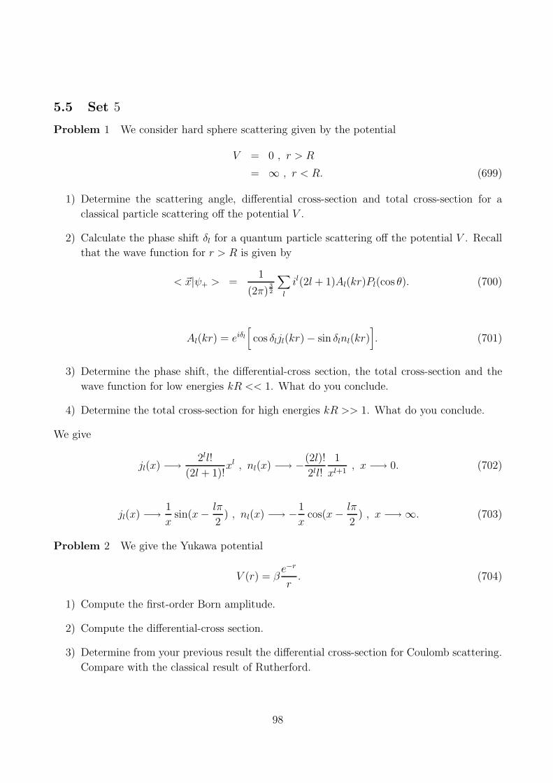
5.5 Set 5
Problem 1 We consider hard sphere scattering given by the potential
V = 0 , r > R
= ∞ , r < R. (699)
1) Determine the scattering angle, differential cross-section and total cross-section for a
classical particle scattering off the potential V .
2) Calculate the phase shift δl for a quantum particle scattering off the potential V . Recall
that the wave function for r > R is given by
< ~x|ψ+ > =1
(2π)32
∑
l
il(2l + 1)Al(kr)Pl(cos θ). (700)
Al(kr) = eiδl[
cos δljl(kr) − sin δlnl(kr)]
. (701)
3) Determine the phase shift, the differential-cross section, the total cross-section and the
wave function for low energies kR << 1. What do you conclude.
4) Determine the total cross-section for high energies kR >> 1. What do you conclude.
We give
jl(x) −→2ll!
(2l + 1)!xl , nl(x) −→ −(2l)!
2ll!
1
xl+1, x −→ 0. (702)
jl(x) −→1
xsin(x− lπ
2) , nl(x) −→ −1
xcos(x− lπ
2) , x −→ ∞. (703)
Problem 2 We give the Yukawa potential
V (r) = βe−r
r. (704)
1) Compute the first-order Born amplitude.
2) Compute the differential-cross section.
3) Determine from your previous result the differential cross-section for Coulomb scattering.
Compare with the classical result of Rutherford.
98
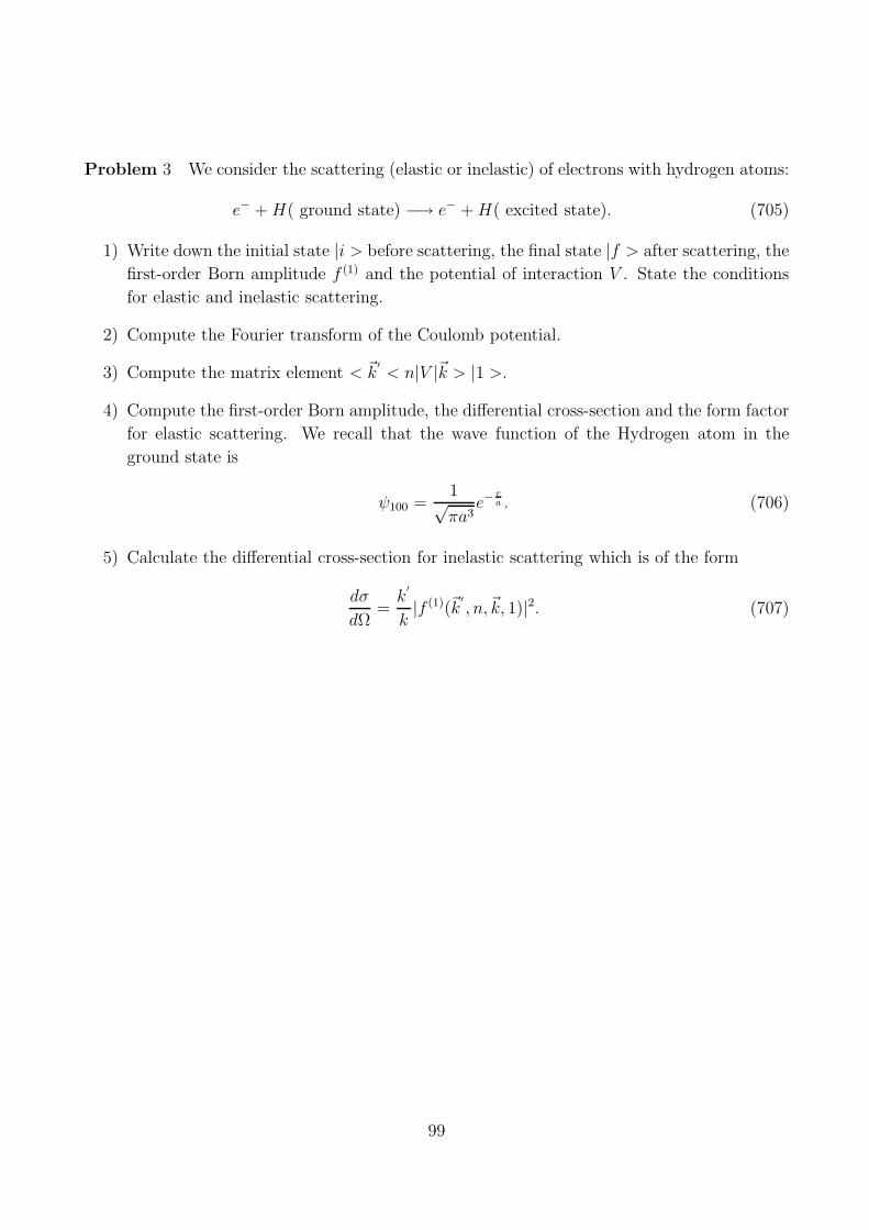
Problem 3 We consider the scattering (elastic or inelastic) of electrons with hydrogen atoms:
e− +H( ground state) −→ e− +H( excited state). (705)
1) Write down the initial state |i > before scattering, the final state |f > after scattering, the
first-order Born amplitude f (1) and the potential of interaction V . State the conditions
for elastic and inelastic scattering.
2) Compute the Fourier transform of the Coulomb potential.
3) Compute the matrix element < ~k′< n|V |~k > |1 >.
4) Compute the first-order Born amplitude, the differential cross-section and the form factor
for elastic scattering. We recall that the wave function of the Hydrogen atom in the
ground state is
ψ100 =1√πa3
e−ra . (706)
5) Calculate the differential cross-section for inelastic scattering which is of the form
dσ
dΩ=k
′
k|f (1)(~k
′
, n,~k, 1)|2. (707)
99
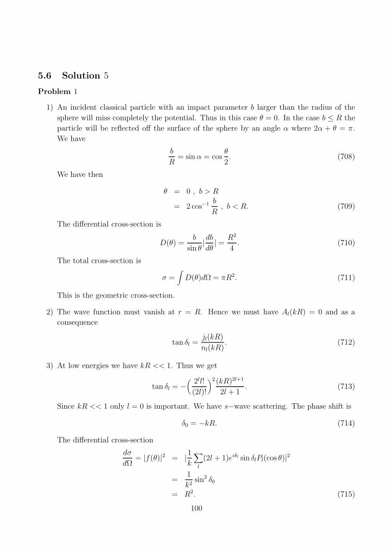
5.6 Solution 5
Problem 1
1) An incident classical particle with an impact parameter b larger than the radius of the
sphere will miss completely the potential. Thus in this case θ = 0. In the case b ≤ R the
particle will be reflected off the surface of the sphere by an angle α where 2α + θ = π.
We have
b
R= sinα = cos
θ
2. (708)
We have then
θ = 0 , b > R
= 2 cos−1 b
R, b < R. (709)
The differential cross-section is
D(θ) =b
sin θ|dbdθ
| =R2
4. (710)
The total cross-section is
σ =∫
D(θ)dΩ = πR2. (711)
This is the geometric cross-section.
2) The wave function must vanish at r = R. Hence we must have Al(kR) = 0 and as a
consequence
tan δl =jl(kR)
nl(kR). (712)
3) At low energies we have kR << 1. Thus we get
tan δl = −(
2ll!
(2l)!
)2 (kR)2l+1
2l + 1. (713)
Since kR << 1 only l = 0 is important. We have s−wave scattering. The phase shift is
δ0 = −kR. (714)
The differential cross-section
dσ
dΩ= |f(θ)|2 = |1
k
∑
l
(2l + 1)eiδl sin δlPl(cos θ)|2
=1
k2sin2 δ0
= R2. (715)
100

The total-cross section is
σ =∫
dΩdσ
dΩ= 4πR2. (716)
This is four times the geometric cross-section. It is equal to the area of the sphere of
radius R. The quantum particle feels its way around the whole sphere.
In this case we have
< ~x|ψ+ > =1
(2π)32
A0(kr) =1
(2π)32
e−ikRsin k(r − R)
kr. (717)
4) For high energy scattering we have kR >> 1. We compute
sin2 δl =tan2 δl
1 + tan2 δl=
j2l (kR)
j2l (kR) + n2
l (kR). (718)
Explicitly
sin2 δl = sin2(kR− lπ
2) (719)
The total cross-section is given by the equation
k2
4πσ =
∑
l
(2l + 1)(sin δl)2. (720)
We remark the identity sin2 δl+1 = 1 − sin2 δl. Thus for even values of l starting from
l = 0 we have sin2 δl = sin2 kR whereas for odd values of l starting from l = 1 we have
sin2 δl = cos2 kR. Thus we get
k2
4πσ =
1
2
∑
l
(2l + 1) − 1
2cos 2kR
(
∑
l even
(2l + 1) −∑
l odd
(2l + 1))
. (721)
We now make the assumption that only angular momenta up to lmax = N − 1 where
N = kR will contribute. We then obtain
1
4πR2σ =
1
2− 1
2Ncos 2kR. (722)
The second term is negligible in the limit of high energies, i.e. when N −→ ∞. We obtain
therefore
σ = 2πR2. (723)
This is twice the geometric cross-section.
101
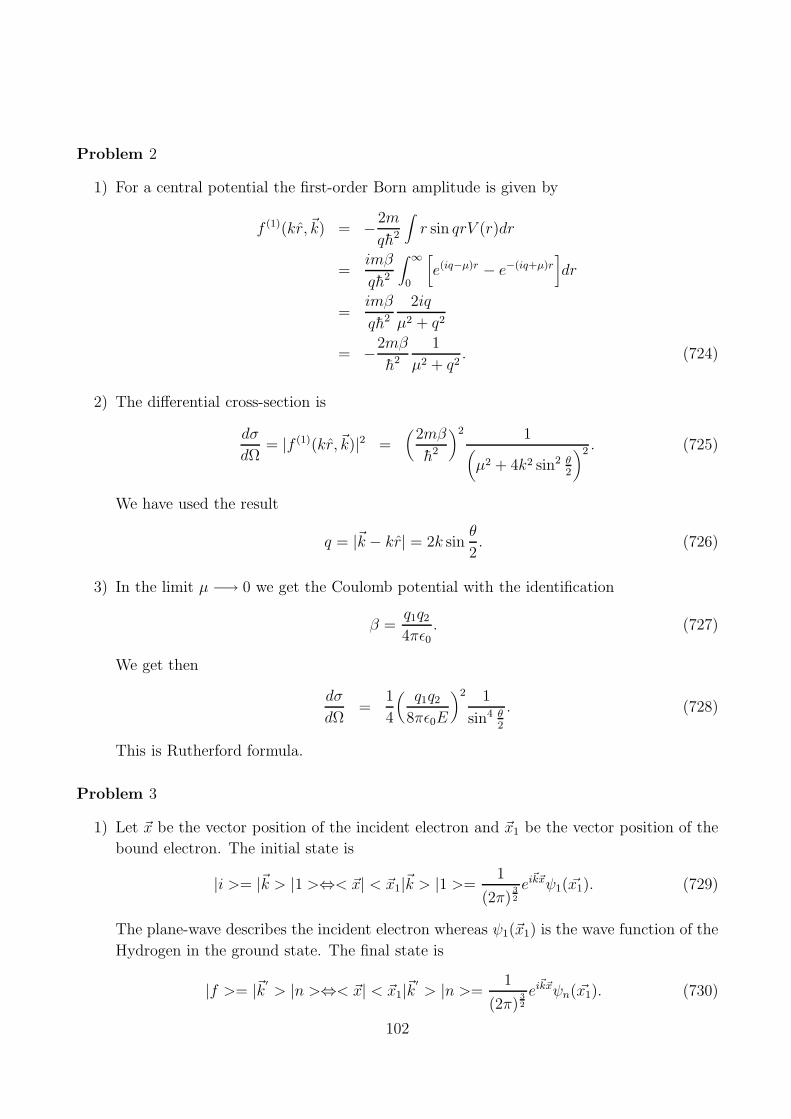
Problem 2
1) For a central potential the first-order Born amplitude is given by
f (1)(kr,~k) = −2m
qh2
∫
r sin qrV (r)dr
=imβ
qh2
∫ ∞
0
[
e(iq−µ)r − e−(iq+µ)r]
dr
=imβ
qh2
2iq
µ2 + q2
= −2mβ
h2
1
µ2 + q2. (724)
2) The differential cross-section is
dσ
dΩ= |f (1)(kr,~k)|2 =
(
2mβ
h2
)2 1(
µ2 + 4k2 sin2 θ2
)2 . (725)
We have used the result
q = |~k − kr| = 2k sinθ
2. (726)
3) In the limit µ −→ 0 we get the Coulomb potential with the identification
β =q1q24πǫ0
. (727)
We get then
dσ
dΩ=
1
4
(
q1q28πǫ0E
)2 1
sin4 θ2
. (728)
This is Rutherford formula.
Problem 3
1) Let ~x be the vector position of the incident electron and ~x1 be the vector position of the
bound electron. The initial state is
|i >= |~k > |1 >⇔< ~x| < ~x1|~k > |1 >=1
(2π)32
ei~k~xψ1( ~x1). (729)
The plane-wave describes the incident electron whereas ψ1(~x1) is the wave function of the
Hydrogen in the ground state. The final state is
|f >= |~k′
> |n >⇔< ~x| < ~x1|~k′
> |n >=1
(2π)32
ei~k~xψn( ~x1). (730)
102
The ψn(~x1) is the wave function of the Hydrogen in the nth energy level. For elastic
scattering we must have n = 1 and ~k′= kr.
The first-order Born amplitude in this case is
f (1)(k′
, n,~k, 1) = −m
h2 (2π)2 < ~k′
< n|V |~k > |1 > . (731)
The potential is (with r = |~x|)
V =1
4πǫ0
(
− e2
r+
e2
|~x− ~x1|
)
. (732)
2) The Fourier Transform of the Coulomb potential is
∫
d3xei~q~x1
r= −2πi
qLimµ−→0
∫
dr[
e(iq−µ)r − e−(iq+µ)r]
= −2πi
q.2iq
q2
=4π
q2. (733)
3) We compute (with ~q = ~k − ~k′)
< ~k′
< n|V |~k > |1 >=1
(2π)3
∫
d3xd3x1ei~q~x 1
4πǫ0
(
− e2
r+
e2
|~x− ~x1|
)
ψ∗n(~x1)ψ1(~x1). (734)
The first term is
1
(2π)3
∫
d3xd3x1ei~q~x 1
4πǫ0
(
− e2
r
)
ψ∗n(~x1)ψ1(~x1) =
1
(2π)3δn1
−e24πǫ0
∫
d3xei~q~x1
r
=1
(2π)3δn1
−e24πǫ0
4π
q2. (735)
The second term is
1
(2π)3
∫
d3xd3x1ei~q~x 1
4πǫ0
(
e2
|~x− ~x1|
)
ψ∗n(~x1)ψ1(~x1) =
1
(2π)3
e2
4πǫ0
∫
d3x1ψ∗n(~x1)ψ1(~x1)
∫
d3xei~q~x1
|~x− ~x1|=
1
(2π)3
e2
4πǫ0
∫
d3x1ψ∗n(~x1)ψ1(~x1)
∫
d3xei~q(~x+~x1)1
r=
1
(2π)3
e2
4πǫ0Fn(~q)
4π
q2. (736)
103
The function Fn(~q) is known as the form factor for the excitation |1 > to |n >:
Fn(~q) =∫
d3x1ψ∗n(~x1)ψ1(~x1)e
i~q~x1
= < n|ei~q~x1 |1 > . (737)
Remark that ei~q~x1 is the Fourier transform of the electron density corresponding to the
bound electron found at ~x1 which is given by
ρ(~x) = δ3(~x− ~x1). (738)
We get then
< ~k′
< n|V |~k > |1 >=1
(2π)3
e2
4πǫ0
4π
q2(−δn1 + Fn(~q)). (739)
4) Thus for elastic scattering we get
f (1)(kr, n,~k, 1) = −2me2
h2q2
1
4πǫ0(−1 + F1(~q)). (740)
The differential cross-section is
dσ
dΩ= |f (1)(kr, 1, ~k, 1)|2 =
(
2me2
h2q2
)2( 1
4πǫ0
)2
(−1 + F1(~q)). (741)
The form factor in this case is
F1(~q) =∫
d3x1ψ∗1(~x1)ψ1(~x1)e
i~q~x1
=∫
r2 sin θdrdθdφe−2ra eiqr cos θ
= − 2i
a3q
∫
rdr[
e(iq−2a)r − e−(iq+ 2
a)r]
= − 2i
a3q
8iqa
(q2 + 4a2
)2
=16
(4 + a2q2)2. (742)
5) For inelastic scattering the formula for the differential cross-section is modified to
dσ
dΩ=k
′
k|f (1)(~k
′
, n,~k, 1)|2 =k
′
k
(
2me2
h2q2
)2( 1
4πǫ0
)2
(Fn(~q)). (743)
104
6 CHAPTER 6: Time-Dependent Perturbation Theory
6.1 The Dirac Interaction Picture
We consider a time-dependent Hamiltonian H of the form
H = H0 + V (t). (744)
The time-independent Hamiltonian H0 corresponds to an exactly solvable problem, viz
H0|n >= En|n > . (745)
The time-dependent potential V (t) is assumed to be small. The initial state vector at time
t = 0 is assumed to be of the form
|ψ(0) >=∑
n
cn(0)|n > . (746)
For t > 0 the state vector takes the general form
|ψ(t) >=∑
n
cn(t)e− iEnt
h |n > . (747)
The phase e−iEnt/h is the usual time-dependent part of the wave function which is present even
if V is independent of time. The unknown are the probability amplitudes cn(t) which depend
on time only because V depend on time. This is not a stationary problem in the sense that
the time-dependent perturbation V (t) can cause transitions between the quantum states |n >.
For example if we start at time t = 0 from the state |ψ(0) >= |i >, i.e. from an eigenstate of
H0 then at later times t > 0 we can find the system in other states |j >, j 6= i. For V = 0 we
will have cj(t) = ci(0)δij and thus the system remains in the state |i > for all times whereas for
V 6= 0 we will find that cj(t) 6= 0 in general and hence there is a probability of transition from
|i > to |j >.
It is very useful to remove the phase e−iEnt/h which is always there anyway from our sub-
sequent analysis. Towards this we introduce the Dirac interaction picture. Let us recall that
the state vector |ψ(t) > is the state vector in the Schrodinger picture. The state vector in the
Heisenberg picture reads
|ψ >= eihHt|ψ(t) > . (748)
Given any operator O in the Schrodinger picture the Heisenberg picture operator is
O(t) = eihHtOe−
ihHt. (749)
The so-called Dirac interaction picture is defined by the state vector and operator given by
|ψ(t) >I= eihH0t|ψ(t) > . (750)
105

OI(t) = eihH0tOe−
ihH0t. (751)
We can immediately compute
ih∂
∂t|ψ(t) >I = −H0|ψ(t) > +e
ihH0t(H0 + V )|ψ(t) >
= VI(t)|ψ(t) >I . (752)
The expansion (747) becomes
|ψ(t) >I=∑
n
cn(t)|n > . (753)
Thus we get immediately
ihdcm(t)
dt=∑
n
cn(t)eiωmntVmn. (754)
ωmn =Em −En
h, Vmn =< m|V |n > . (755)
6.2 Two-State Problems
In this case we have
ihdc1(t)
dt=∑
n
cn(t)eiω1ntV1n = c1(t)V11 + c2(t)e
−iω0tV12. (756)
ihdc2(t)
dt=∑
n
cn(t)eiω2ntV2n = c1(t)e
iω0tV21 + c2(t)V22. (757)
ω0 =E2 −E1
h, E2 > E1. (758)
We assume that
V11 = V22 = 0. (759)
In this case we get
dc1(t)
dt= − i
hc2(t)e
−iω0tV12. (760)
dc2(t)
dt= − i
hc1(t)e
iω0tV21. (761)
106
We consider sinusoidal perturbations of the form
V12 = V ∗21 = γeiωt. (762)
The above coupled differential equations become
dc1(t)
dt= −iγ
hc2(t)e
−i(ω0−ω)t. (763)
dc2(t)
dt= −iγ
hc1(t)e
i(ω0−ω)t. (764)
From these two equations we can derive the second order differential equation
d2c1(t)
dt+ i(ω − ω0)
dc1dt
+γ2
h2 c1(t) = 0. (765)
We take the ansatz
c1 = eiω−ω0
2tc1. (766)
We find
d2c1(t)
dt+[
(ω − ω0)2
4+γ2
h2
]
c1(t) = 0. (767)
In other words
c1 = eiω−ω0
2t[
A cosωrt+B sinωrt]
. (768)
The frequency ωr is called Rabi flopping frequency and it is given by
ω2r =
(ω − ω0)2
4+γ2
h2 . (769)
The differential equation (763) can now be rewritten as
−iγhc2 = i
ω − ω0
2e−i
ω−ω02
t[
A cosωrt+B sinωrt]
+ ωre−iω−ω0
2t[
− A sinωrt+B cosωrt]
. (770)
We use the initial conditions
c1(0) = 1 , c2(0) = 0. (771)
We find
A = 1 , B = −iω − ω0
2ωr. (772)
Hence
c1 = eiω−ω0
2t[
cosωrt− iω − ω0
2ωrsinωrt
]
. (773)
107

c2 = − i
ωr
γ
he−i
ω−ω02
t sinωrt. (774)
The system starts initially in the state |1 >. The probability of finding the system at time t in
the state |2 > is given by
|c2|2 =1
ω2r
γ2
h2 sin2 ωrt =1
ω2r
γ2
h2
1
2(1 − cos 2ωrt). (775)
This is Rabi’s formula. The probability of finding the system in the state |2 > oscillates in time
with a frequency 2ωr. The amplitude of oscillation is maximum at ω = ω0. This is a resonance
behavior.
Resonance is defined by
ω = ω0 , ωr =γ
h. (776)
The transition probability at resonance becomes
|c2|2 =1
2(1 − cos 2ωrt). (777)
From time t = 0 to t = πh/2γ the probability of finding the system in |2 > increases until it
reaches 1. Recall that the energy E2 is greater than the energy E1. Thus during this time the
system absorbs energy from the perturbation until at time t = πh/2γ only the state |2 > is
populated. From t = πh/2γ to t = πh/γ the probability |c2|2 decreases and thus the system
gives up energy to the perturbation until at at time t = πh/γ only the state |1 > is populated.
This emission-absorption cycle continues indefinitely.
Away from resonance the maximum of the transition probability |c2|2 is given by
|c2|2 =1
ω2r
γ2
h2 sin2 ωrt ≤ |c2|2max =γ2
h2
(ω−ω0)2
4+ γ2
h2
. (778)
This is a resonance curve with a peak at ω = ω0. The frequencies corresponding to a probability
|c2|2 = 1/2 are ω = ω0±2γ/h. Therefore the width at half maxima is 4γ/h. Clearly the widths
become smaller, i.e. we get narrower resonance peaks for weaker potentials.
Among the applications of this two-level system we only mention nuclear magnetic resonance
and microwave amplification by stimulated emission of radiation or MASERS.
6.3 Dyson Series
In the interaction picture Schrodinger equation reads
ih∂
∂t|ψ(t) >I = VI(t)|ψ(t) >I . (779)
The time evolution operator in the interaction picture is defined by
|ψ(t) >I= UI(t, t0)|ψ(t0) >I . (780)
108
From the other hand
|ψ(t) >I = eihH0t|ψ(t) >
= eihH0tU(t, t0)e
− ihH0t0 |ψ(t0) >I . (781)
Hence
UI(t, t0) = eihH0tU(t, t0)e
− ihH0t0 . (782)
This obeys the differential equation
ihd
dtUI(t, t0) = VI(t)UI(t, t0). (783)
The initial condition reads
UI(t0, t0) = 1. (784)
A solution is given by the integral equation
UI(t, t0) = 1 − i
h
∫ t
t0dt1VI(t1)UI(t1, t0). (785)
We can iterate this equation as follows
UI(t, t0) = 1 − i
h
∫ t
t0dt1VI(t1)
[
1 − i
h
∫ t1
t0VI(t2)UI(t2, t0)dt2
]
= 1 +(−ih
)∫ t
t0dt1VI(t1) +
(−ih
)2 ∫ t
t0dt1
∫ t1
t0dt2VI(t1)VI(t2)U(t2, t0). (786)
Iterating to an arbitrary order we get
UI(t, t0) = 1 +(−ih
)∫ t
t0dt1VI(t1) +
(−ih
)2 ∫ t
t0dt1
∫ t1
t0dt2VI(t1)VI(t2) + ...
+(−ih
)n ∫ t
t0dt1
∫ t1
t0dt2...
∫ tn−1
t0dtnVI(t1)VI(t2)...VI(tn) + .... (787)
This solution is known as Dyson series.
Recall that
|ψ(t) >I=∑
n
cn(t)|n > . (788)
We compute immediately that
cn(t) =< n|UI(t, t0)|ψ(t0) >I . (789)
We choose the initial state such that
|ψ(t0) >I= |i >⇔ |ψ(t0) >= e−ihEit0 |i > . (790)
109

The transition amplitude becomes
cn(t) =< n|UI(t, t0)|i >= eih(Ent−Eit0) < n|U(t, t0)|i > . (791)
The transition probability is
Pi−→n(t) = |cn(t)|2 = | < n|UI(t, t0)|i > |2 = | < n|U(t, t0)|i > |2. (792)
This is given by
Pi−→n(t) = |c(0)n (t) + c(1)n (t) + c(2)n (t) + ...|2. (793)
c(0)n (t) = δni. (794)
c(1)n (t) =(−ih
) ∫ t
t0dt1 < n|VI(t1)|i >
=(−ih
) ∫ t
t0dt1e
iωnit1Vni(t1). (795)
c(2)n (t) =(−ih
)2 ∫ t
t0dt1
∫ t1
t0dt2 < n|VI(t1)VI(t2)|i >
=(−ih
)2 ∫ t
t0dt1
∫ t1
t0dt2
∑
m
eiωnmt1eiωmit2Vnm(t1)Vmi(t2). (796)
ωij =Ei − Ej
h, Vij(t) =< i|V (t)|j > . (797)
6.4 Fermi’s Golden Rule
We consider a constant perturbation of the form
V (t) = 0 , t < 0
= V , t ≥ 0. (798)
The operator V depends on time only implicitly. We compute (with t0 = 0)
c(1)n (t) =(−ih
) ∫ t
0dt1e
iωnitVni(t)
= Vni1 − eiωnit
En −Ei. (799)
Thus
|c(1)n (t)|2 =2|Vni|2
(En − Ei)2(1 − cosωnit). (800)
110
Thus for n 6= i the first-order transition probability at time t is
Pi−→n(t) =4|Vni|2
(En − Ei)2sin2 (En − Ei)t
2h. (801)
This depends on 1) the matrix component Vni between the initial state |i > and the final state
|n > and on 2) the energy difference En − Ei = hωni between the two states. The time t is
the time interval during which the perturbation has been turned on. For a fixed value of t we
study the probability Pi−→n(t) as a function of ωni, viz Pi−→n(t) = P (ωni). The maximum of
this probability is at ωni = 0 where it is proportional to t2 and it vanishes at ωni = 2nπ/t,
n = 1, 2.... There are smaller peaks at ωni = (2n + 1)π/t, n = 1, 2.... Thus the width of the
probability P (ωni) is 1/t. In other words |c(1)n |2 for very large times is not negligible only for
states |n > with energies around En, viz
|En −Ei|t ∼ 2πh. (802)
This uncertainty relation means in particular that for t −→ 0 we obtain a broader peak and
thus transitions with nonconservation of energy are probable whereas for t −→ ∞ we obtain a
narrower peak and the transitions with En ≃ Ei are the most probable.
The area under the curve P (ωni) is therefore proportional to t2 × 1/t = t which should be
equal to the total probability for the transition from the initial state |i > to the final states
|n > with energies centered around En. This can be made more precise as follows. The total
probability is the transition probabilities summed over final states which have energies En ≃ Ei.
This is given by
∑
n:En≃Ei
|c(1)n |2. (803)
We assume that the final states constitute a continuum. We introduce the density of final states
ρ(E). In other words ρ(E)dE is the number of states with energy between E and E + dE. We
can then replace the above total probability with the integral
∫
dEnρ(En)|c(1)n |2 =∫
dEnρ(En)4|Vni|2
(En − Ei)2sin2 (En − Ei)t
2h. (804)
For very large times we can use the identity
limt−→∞sin2 tx
tx2= πδ(x). (805)
We get
∑
n:En≃Ei
|c(1)n |2 =∫
dEnρ(En)|c(1)n |2 =∫
dEnρ(En)2πt
h|Vni|2δ(En − Ei)
=[
ρ(En)2πt
h|Vni|
2]
En=Ei
. (806)
111
The bar over |Vni|2 is to indicate that for states |n > with nearly equal energy En the matrix
elements Vni are not necessarily the same.
The transition rate is the transition probability per unit time. This is defined by
wi−→[n] =d
dt
∑
n:En≃Ei
|c(1)n |2 =2π
h
[
|Vni|2ρ(En)
]
En=Ei
. (807)
This is Fermi’s golden rule. The above formula can also be written as
wi−→n =2π
h|Vni|2ρ(En)δ(En −Ei)dEn. (808)
The second-order correction to the transition amplitude is
c(2)n (t) =(−ih
)2 ∫ t
0dt1
∫ t1
0dt2
∑
m
eiωnmt1eiωmit2VnmVmi
=i
h
∑
m
VnmVmiEm − Ei
∫ t
0dt1(e
iωnit1 − eiωnmt1)
=∑
m
VnmVmiEi − Em
[
1 − eiωnit
En − Ei− 1 − eiωnmt
En −Em
]
. (809)
The behavior of the first term in this expression at large time t is similar to the behavior of c(1)nwith the replacement Vni −→
∑
m VnmVmi/(Ei − Em). Thus only the states with En ≃ Ei will
contribute significantly. The second term when Em 6= En and Em 6= Ei gives rise to a rapid
oscillation which does not grow with t. The case when Em ≃ Ei with VnmVmi 6= 0 is special and
will not be discussed here. In summary the transition rate including the second-order correction
is
wi−→[n] =d
dt
∑
n:En≃Ei
|c(1)n + c(2)n |2 =2π
h
[
|Vni +∑
m
VnmVmiEi − Em
|2
ρ(En)]
En=Ei
. (810)
We have already mentioned that the first-order term represent an energy-conserving transition.
The second-order term can be understood as the combination of two nonconserving transitions
from |i > to |m > and then from |m > to |n >. These transitions are termed virtual since they
do not conserve energy although there is always an overall conservation of energy between |i >and |n >.
6.5 Emission and Absorption of Radiation
6.5.1 Harmonic Perturbation
We consider the harmonic perturbation
V (t) = V eiωt + V +e−iωt. (811)
112
Again V and V + depend only implicitly on time. At the initial time t = 0 only the eigenstate
|i > of H0 is populated. We compute the first-order amplitude
c(1)n (t) =−ih
∫ t
0dt1e
iωnitVni(t)
=1
h
[
Vni1 − ei(ωni+ω)t
ωni + ω+ V +
ni
1 − ei(ωni−ω)t
ωni − ω
]
. (812)
Recall that for constant perturbation we obtained
c(1)n (t) =1
h
[
Vni1 − eiωnit
ωni
]
. (813)
In other words the only change is
ωni −→ ωni ± ω. (814)
Hence for large times t the probability |c(1)n |2 is important only in the two mutually exclusive
cases
ωni + ω = 0 ⇔ En = Ei − hω. (815)
ωni − ω = 0 ⇔ En = Ei + hω. (816)
Clearly the energy of the system alone is not conserved. It is the combination system plus
external perturbation V (t) which conserves energy. The second case (816) is only possible
if En > Ei, i.e. if En is an excited state. It corresponds to absorption where the system
receives an energy hω from the perturbation V (t). The first case (815) is only possible if
En < Ei, i.e. if Ei is an excited state. It corresponds to stimulated emission where the
system gives up an energy hω to the perturbation V (t). The emission is termed “stimulated”
because it is caused by the perturbation. For example when we shine a light on an atom in
an excited state Ei it can make a transition to the lower state En. In other words the single
incident photon becomes two outgoing photons with the same frequency. This is the principle
of amplification underlying LASER (light amplification by stimulated emission of radiation).
Stimulated emission by electromagnetic interaction was first predicted by Einstein.
The Fermi’s Golden rule in this case read
wstim−emisi−→[n] =
2π
h
[
|Vni|2ρ(En)
]
En=Ei−hω. (817)
wabsoi−→[n] =
2π
h
[
|V +ni |
2ρ(En)
]
En=Ei+hω. (818)
From the result |Vni|2 = |V +in |2 we get detailed balance which expresses the symmetry between
absorption and stimulated emission. This reads
wstim−emisi−→[n]
ρ(En)=wabson−→[i]
ρ(Ei). (819)
113
6.5.2 Stimulated Emission and Absorption
The Hamiltonian of a charge q moving under the influence of an electric field ~E = −~∇φ−∂ ~A/∂t and a magnetic field ~B = ~∇× ~A is given by
H =1
2m(~p− q ~A)2 + qφ. (820)
The φ and ~A are the scalar and vector potentials respectively. We impose the Coulomb gauge
condition
~∇ ~A = 0. (821)
The Hamiltonian can be rewritten as
H =~p2
2m− q
m~A~p+
q2 ~A2
2m+ qφ. (822)
We consider the field of a monochromatic plane wave given by
φ = 0 , ~A = 2ǫA0 cos(kn~x− ωt). (823)
The direction of propagation is n and the direction of polarization is ǫ. The wavenumber is
k = ω/c. The gauge condition ~∇ ~A = 0 means that the wave is transverse, i.e. ǫn = 0. The
Hamiltonian becomes
H =~p2
2m+ V eiωt + V +e−iωt. (824)
V = −qA0
mǫ~pe−ikn~x. (825)
In the above equation we have neglected the diamagnetic term q2 ~A2/2m and used the fact that
ǫ~p exp(ikn~x) = exp(ikn~x)ǫ~p.
The term eiωtV corresponds to stimulated emission whereas the term e−iωtV + corresponds
to absorption. In the remainder we will study absorption in more detail. We compute (with
q = e)
|V +ni | =
e2A20
m2|ǫ < n|~peikn~x|i > |2. (826)
We can make the approximation that the wavelength of the radiation is much larger than the
size of the atoms, viz |kn~x| = 2π|n~x/λ| << 1. Hence we can approximate the exponential by
1. This is the electric dipole approximation. We get
|V +ni | =
e2A20
m2|ǫ < n|~p|i > |2. (827)
114
From the identity [x,H0] = ihpx/m we calculate that < n|~p|i >= imωni < n|~x|i >. Hence we
obtain
|V +ni | = A2
0ω2ni|ǫ < n|~P |i > |2. (828)
The vector ~P is the electric dipole moment defined by
~P = e~x. (829)
The electric field ~E of the above monochromatic plane wave is given by ~E = −ǫ(2ωA0) sin(kn~x−ωt). The energy density (energy per unit volume) in an electromagnetic wave is u = (ǫ0E
2 +
B2/µ0)/2 = ǫ0E2. Thus the average over a full cycle is u = 2ǫ0ω
2A20. Hence we get (we also
use the fact that ωni = ω)
|V +ni | =
u
2ǫ0|ǫ < n|~P |i > |2. (830)
We take the average of this expression over all incident directions n and all polarization di-
rections ǫ. We work in spherical coordinates. The vectors n and ǫ are perpendicular. We
choose the z axis along the propagation direction n. We choose the y axis such that the vector
< n|~P |i > lies in the zy plane. The x axis is then fixed. The angle between n and < n|~P |i >is θ and the angle between the x axis and ǫ is φ. We have then
ǫ = cosφi+ sinφj , < n|~P |i >= | < n|~P |i > |(cos θk + sin θj). (831)
The desired average is given by the integral
|V +ni | =
u
2ǫ0| < n|~P |i > |2 1
4π
∫
sin2 φ sin2 θ sin θdθdφ
=u
6ǫ0| < n|~P |i > |2. (832)
Clearly
< n|~P |i > |2 =< n|Px|i >2 + < n|Py|i >2 + < n|Pz|i >2 . (833)
We write the absorption rate (818) as
wabsoi−→n =
2π
h|V +ni |
2δ(En −Ei − hω)ρ(En)dEn
=π
3ǫ0h2 | < n|~P |i > |2δ(ωni − ω)uρ(En)dEn. (834)
The electromagnetic wave is not perfectly monochromatic so it comes with a finite frequency
width. Recall that ρ(En)dEn is the number of final states with energy between En = h(ω+Ei/h)
and En + dEn = h(ω + dω + Ei/h) where Ei is kept fixed. Thus we see that ρ(En)dEn is the
number of electromagnetic modes with frequency between ω and ω + dω. The energy density
115

in the electromagnetic mode with frequency ω is u. Hence uρ(En)dEn is the energy density in
the electromagnetic modes with frequency between ω and ω + dω. We write this as
uρ(En)dEn = ρu(ω)dω (835)
We get the final result
wabsoi−→n =
π
3ǫ0h2 | < n|~P |i > |2δ(ωni − ω)ρu(ω)dω. (836)
This can also be written as
wabsoi−→[n] =
π
3ǫ0h2
[
| < n|~P |i > |2ρu(ω)]
ω=ωni
. (837)
116
6.6 Set 6
Problem 1 The energies and wave functions of the one-dimensional infinite square well are
given by
En =n2π2h2
2ma2, ψn(x) =
√
2
asin
nπx
a, n = 1, 2, 3, ... (838)
A time-dependent perturbation is introduced during the time interval T such that the potential
becomes
V (x) = V0 , 0 ≤ x ≤ a
2
V (x) = 0 ,a
2≤ x ≤ 0
V (x) = ∞ , otherwise. (839)
At t = 0 the system is in the ground state n = 1. What is the probability that at time t = T
the system jumps to the first excited state n = 2.
Problem 2
1) In the photoelectric effect the initial state of the electron is an atomic bound state with
energy Ei > 0 whereas the final state is a free continuum state with energy around En < 0.
Write down Fermi’s Golden rule in this case.
2) Derive an expression for the density of final states ρ(En). Use the box normalization of
plane-wave states given by
< ~x|~k >=1
L32
ei~k~x. (840)
In this case the allowed values of kx, ky and kz are
kx =2πnxL
, ky =2πnyL
, kz =2πnzL
. (841)
The orthonormalization and completeness relations are
< ~k′ |~k >= δ~k′ ,~k. (842)
∑
~k
|~k >< ~k| = 1. (843)
3) Derive the differntial cross-section of the process defined by
dσ
dΩ=hω
uwabsoi−→n. (844)
117
Problem 3 We place a one-dimensional harmonic oscillator under the influence of a spatially
uniform time-dependent force given by
F (t) =F0τ
ω(τ 2 + t2). (845)
At t = −∞ the harmonic oscillator is in the ground state. Compute the probability that at
time t = +∞ the harmonic oscillator will be found in the first excited state.
Problem 4 A scattering process can be viewed as a transition process from the initial free
state |~k > at time t = −∞ (remote past) into a group of final states |~k′> with momentum
directions within a solid angle dΩ = d3k′/(k
′2dk′) at time t. We will only consider elastic
scattering for which k′= k. In this transition process the interaction is zero at time t = −∞ and
then it increases slowly (adiabatically) with time. The time-dependent potential can therefore
be taken to be
V (t) = V eηt. (846)
In this equation η is a very small positive number which needs to be send to zero at the end of
the calculation.
1) Show that the transition probability is till given by Fermi’s Golden rule.
2) Compute the transition rate into a group of final states |~k′> with energy between Ek′
and Ek′ + dEk′ . Use the density of final states obtained in problem 2.
3) Compute the incident flux given by
|~j| =h
m|Im(ψ∗~∇ψ)| , ψ =< ~x|~k > . (847)
4) Derive the differential cross-section. Compare the result with the first-order Born approx-
imation.
118
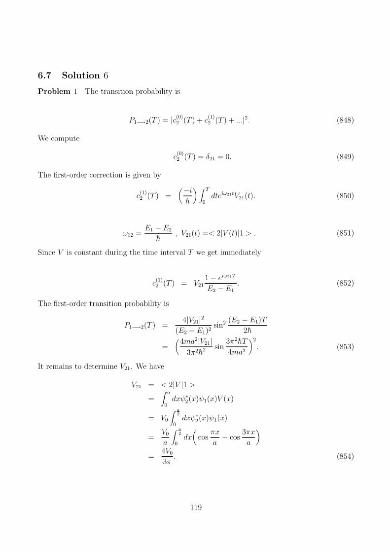
6.7 Solution 6
Problem 1 The transition probability is
P1−→2(T ) = |c(0)2 (T ) + c(1)2 (T ) + ...|2. (848)
We compute
c(0)2 (T ) = δ21 = 0. (849)
The first-order correction is given by
c(1)2 (T ) =
(−ih
) ∫ T
0dteiω21tV21(t). (850)
ω12 =E1 − E2
h, V21(t) =< 2|V (t)|1 > . (851)
Since V is constant during the time interval T we get immediately
c(1)2 (T ) = V21
1 − eiω21T
E2 − E1. (852)
The first-order transition probability is
P1−→2(T ) =4|V21|2
(E2 − E1)2sin2 (E2 − E1)T
2h
=(
4ma2|V21|3π2h2 sin
3π2hT
4ma2
)2
. (853)
It remains to determine V21. We have
V21 = < 2|V |1 >=
∫ a
0dxψ∗
2(x)ψ1(x)V (x)
= V0
∫ a2
0dxψ∗
2(x)ψ1(x)
=V0
a
∫ a2
0dx(
cosπx
a− cos
3πx
a
)
=4V0
3π. (854)
119

Problem 2
1) The absorption rate without 1) the electric dipole approximation and without 2) averaging
over all incident directions n and all polarization directions ǫ is given by
wabsoi−→n =
πe2
hǫ0m2ω2|ǫ < n|~peiω
cn~x|i > |2δ(En − Ei − hω)uρ(En)dEn. (855)
This is the probability per unit time that a charge e which starts in the state |i > with
energy Ei = hωi will jump at time t to the state |n > with energy En = hωn under the
influence of an electromagnetic field (time-dependent perturbation) of frequency ω. In
above ~p is the momentum of the charge, u is the energy density (energy per unit volume)
in the field and ρ(En)dEn is the number of final states with energy between En and
En + dEn.
2) In the photoelectric effect the initial state of the electron is an atomic bound state with
energy Ei > 0 whereas the final state is a free continuum state with energy around En < 0.
Thus
En =h2~k2
2m, |n >= |~k > . (856)
The number of states with momentum between h~k and h(~k + d~k) is equal to the number
of states with energy between En and En + dEn with momentum direction within a solid
angle dΩ = d3k/(k2dk). Using box normalization of plane-wave states we have
< ~x|~k >=1
L32
ei~k~x. (857)
In this case the allowed values of kx, ky and kz are
kx =2πnxL
, ky =2πnyL
, kz =2πnzL
. (858)
Clearly there is one state in a cube of volume (2π/L)3 in momentum space. Thus the
number of states with energy between En and En+dEn with momentum directions within
a solid angle dΩ = d3k/(k2dk) is
ρ(En)dEn =k2dkdΩ
(2πL
)3= (
L
2π)3km
h2 dEndΩ. (859)
3) We get then
wabsoi−→n =
πe2
hǫ0m2ω2|ǫ < ~k|~peiω
cn~x|i > |2δ(En − Ei − hω)u(
L
2π)3km
h2 dEndΩ. (860)
Integrating over En we get (now k =√
2m(Ei + hω)/h2)
wabsoi−→n =
πe2
hǫ0m2ω2|ǫ < ~k|~peiω
cn~x|i > |2u( L
2π)3km
h2 dΩ. (861)
120

We compute
ǫ < ~k|~peiωcn~x|i > =
1
L32
ǫ∫
d3xe−i~k~x+iω
cn~x h
i~∇ψi(~x)
=h
L32
ǫ~k∫
d3xe−i~q~xψi(~x) , ~q = ~k − ω
cn. (862)
Recall that ψi(~x) is the wave function of the bound electron. Thus in the case of the
hydrogen atom ψi(~x) is the ground-state wave function given by
ψi(~x) =1√πa3
e−ra . (863)
We get
ǫ < ~k|~peiωcn~x|i > =
h
L32
ǫ~k8π
a√πa3
1
(q2 + 1a2
)2. (864)
We get finally
wabsoi−→n =
u
hωdΩ(
8e2k
πǫ0mω(ǫ~k)2 1
a5
1
(q2 + 1a2
)4
)
. (865)
We choose n in the z direction and ǫ in the x direction. The vector ~k will be defined by
two angles θ and φ. Then
(ǫ~k)2 = k2x = k2 sin2 θ cos2 φ , q2 = k2 +
ω2
c2− 2
ω
ckz = k2 +
ω2
c2− 2
ω
ck cos θ. (866)
Problem 3 The ground state and the first excited state wave functions of the one-dimensional
harmonic oscillator are given by
ψ0(x) =(
mω
πh
) 14
e−mω2hx2
. (867)
ψ1(x) = a+ψ0(x) =(
mω
πh
) 14
√
2mω
hx e−
mω2hx2
. (868)
The corresponding energies are
E0 =hω
2, E1 =
3hω
2. (869)
The 0th order transition amplitude is
c(0)1 (+∞) = δ10 = 0. (870)
121

The 1st order transition amplitude is
c(1)1 (+∞) = − i
h
∫ ∞
−∞dt eiω10tV10(t)
= − i
h
∫ ∞
−∞dt eiωt < 1|V (t)|0 > . (871)
The force is spatially uniform. Thus the potential is V = −Fx. We compute
< 1|V (t)|0 >=< 1|(−Fx)|0 >= −F√
h
2mω< 1|(a+ a+)|0 >= −F
√
h
2mω. (872)
Hence
c(1)1 (+∞) =
i√2mωh
F0τ
ω
∫ ∞
−∞dt
eiωt
τ 2 + t2
=iF0
ω√
2mωh
∫ ∞
−∞dt
eiωτt
1 + t2. (873)
We introduce Laplace transform
∫ ∞
−∞dteiωτt
1 + t2=
∫ ∞
−∞dt∫ ∞
0dαe−α(1+t2)+iωτt
=∫
dαe−α−(ωτ2)2
1α
∫ ∞
−∞dte−α(t−
iωτ2α
)2
=∫
dαe−α−(ωτ2)2
1α
∫ ∞
−∞dte−αt
2
=∫
dαe−α−(ωτ2)2
1α
√
π
α
=
√
πωτ
2
∫ dα
α12
e−ωτ2
(α+ 1α
)
=
√
πωτ
22K− 1
2(ωτ)
=
√
πωτ
22
√
π
2ωτe−ωτ
= πe−ωτ . (874)
Thus
c(1)1 (+∞) =
iF0
ω√
2mωhπe−ωτ . (875)
The transition probability is
|c(1)1 (+∞)|2 =F 2
0 π2
2mω3he−2ωτ . (876)
122
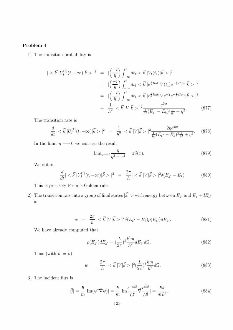
Problem 4
1) The transition probability is
| < ~k′|U (1)
I (t,−∞)|~k > |2 = |(−ih
)∫ t
−∞dt1 < ~k
′ |VI(t1)|~k > |2
= |(−ih
)∫ t
−∞dt1 < ~k
′ |e ihH0t1V (t1)e
− ihH0t1 |~k > |2
= |(−ih
)∫ t
−∞dt1 < ~k
′ |e ihH0t1V eηt1e−
ihH0t1 |~k > |2
=1
h2 | < ~k′ |V |~k > |2 e2ηt
1h2 (Ek′ − Ek)2 1
h2 + η2. (877)
The transition rate is
d
dt| < ~k
′|U (1)I (t,−∞)|~k > |2 =
1
h2 | < ~k′ |V |~k > |2 2ηe2ηt
1h2 (Ek′ −Ek)2 1
h2 + η2. (878)
In the limit η −→ 0 we can use the result
Limη−→0η
η2 + x2= πδ(x). (879)
We obtain
d
dt| < ~k
′ |U (1)I (t,−∞)|~k > |2 =
2π
h| < ~k
′|V |~k > |2δ(Ek′ − Ek). (880)
This is precisely Fermi’s Golden rule.
2) The transition rate into a group of final states |~k′> with energy between Ek′ and Ek′+dEk′
is
w =2π
h| < ~k
′ |V |~k > |2δ(Ek′ − Ek)ρ(Ek′ )dEk′ . (881)
We have already computed that
ρ(Ek′ )dEk′ = (L
2π)3k
′m
h2 dEk′dΩ. (882)
Thus (with k′= k)
w =2π
h| < ~k
′|V |~k > |2( L2π
)3km
h2 dΩ. (883)
3) The incident flux is
|~j| =h
m|Im(ψ∗~∇ψ)| =
h
m|Ime−i
~k~x
L32
~∇ei~k~x
L32
| =hk
mL3. (884)
123
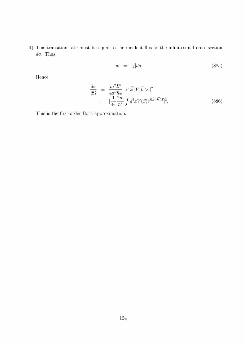
4) This transition rate must be equal to the incident flux × the infinitesimal cross-section
dσ. Thus
w = |~j|dσ. (885)
Hence
dσ
dΩ=
m2L6
4π2h4| < ~k
′ |V |~k > |2
= | 1
4π
2m
h2
∫
d3xV (~x)ei(~k−~k′)~x|2. (886)
This is the first-order Born approximation.
124
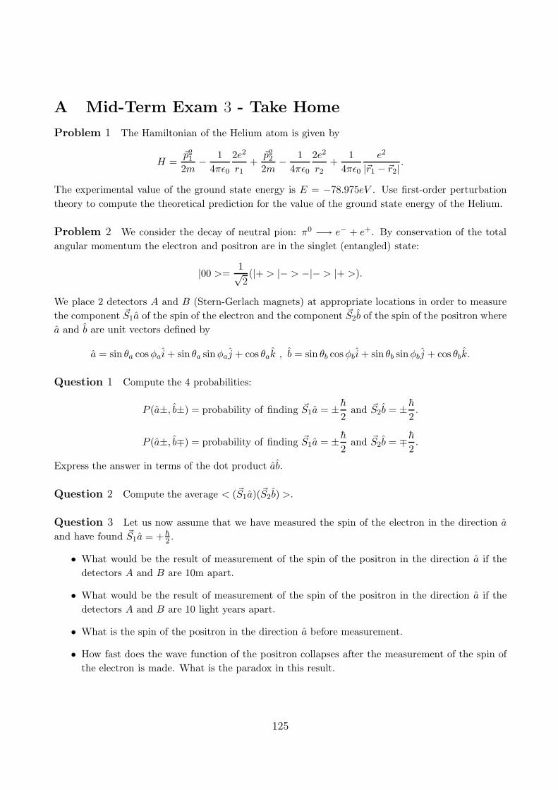
A Mid-Term Exam 3 - Take Home
Problem 1 The Hamiltonian of the Helium atom is given by
H =~p21
2m− 1
4πǫ0
2e2
r1+
~p22
2m− 1
4πǫ0
2e2
r2+
1
4πǫ0
e2
|~r1 − ~r2|.
The experimental value of the ground state energy is E = −78.975eV . Use first-order perturbation
theory to compute the theoretical prediction for the value of the ground state energy of the Helium.
Problem 2 We consider the decay of neutral pion: π0 −→ e− + e+. By conservation of the total
angular momentum the electron and positron are in the singlet (entangled) state:
|00 >=1√2(|+ > |− > −|− > |+ >).
We place 2 detectors A and B (Stern-Gerlach magnets) at appropriate locations in order to measure
the component ~S1a of the spin of the electron and the component ~S2b of the spin of the positron where
a and b are unit vectors defined by
a = sin θa cosφai+ sin θa sinφaj + cos θak , b = sin θb cosφbi+ sin θb sinφbj + cos θbk.
Question 1 Compute the 4 probabilities:
P (a±, b±) = probability of finding ~S1a = ± h2
and ~S2b = ± h2.
P (a±, b∓) = probability of finding ~S1a = ± h2
and ~S2b = ∓ h2.
Express the answer in terms of the dot product ab.
Question 2 Compute the average < (~S1a)(~S2b) >.
Question 3 Let us now assume that we have measured the spin of the electron in the direction a
and have found ~S1a = + h2 .
• What would be the result of measurement of the spin of the positron in the direction a if the
detectors A and B are 10m apart.
• What would be the result of measurement of the spin of the positron in the direction a if the
detectors A and B are 10 light years apart.
• What is the spin of the positron in the direction a before measurement.
• How fast does the wave function of the positron collapses after the measurement of the spin of
the electron is made. What is the paradox in this result.
125
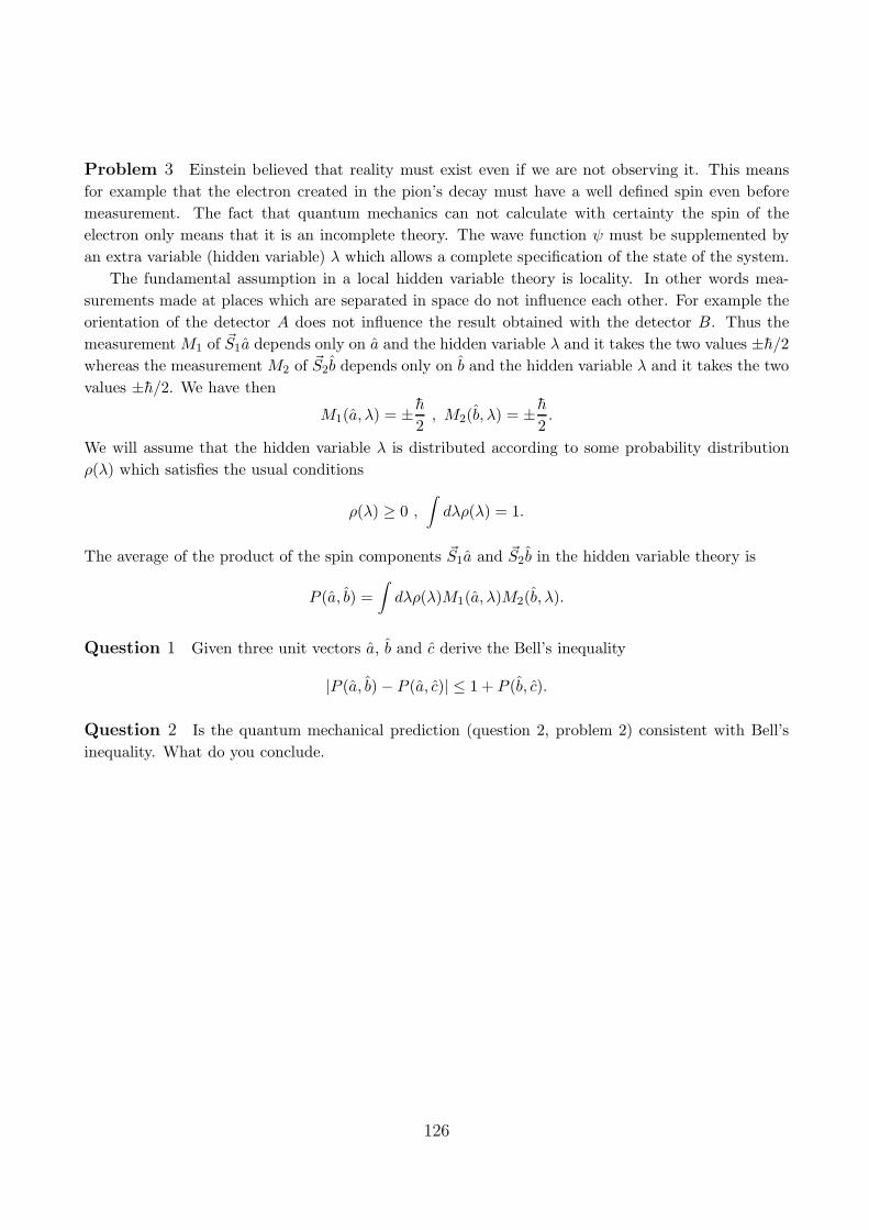
Problem 3 Einstein believed that reality must exist even if we are not observing it. This means
for example that the electron created in the pion’s decay must have a well defined spin even before
measurement. The fact that quantum mechanics can not calculate with certainty the spin of the
electron only means that it is an incomplete theory. The wave function ψ must be supplemented by
an extra variable (hidden variable) λ which allows a complete specification of the state of the system.
The fundamental assumption in a local hidden variable theory is locality. In other words mea-
surements made at places which are separated in space do not influence each other. For example the
orientation of the detector A does not influence the result obtained with the detector B. Thus the
measurement M1 of ~S1a depends only on a and the hidden variable λ and it takes the two values ±h/2whereas the measurement M2 of ~S2b depends only on b and the hidden variable λ and it takes the two
values ±h/2. We have then
M1(a, λ) = ± h2, M2(b, λ) = ± h
2.
We will assume that the hidden variable λ is distributed according to some probability distribution
ρ(λ) which satisfies the usual conditions
ρ(λ) ≥ 0 ,
∫
dλρ(λ) = 1.
The average of the product of the spin components ~S1a and ~S2b in the hidden variable theory is
P (a, b) =
∫
dλρ(λ)M1(a, λ)M2(b, λ).
Question 1 Given three unit vectors a, b and c derive the Bell’s inequality
|P (a, b) − P (a, c)| ≤ 1 + P (b, c).
Question 2 Is the quantum mechanical prediction (question 2, problem 2) consistent with Bell’s
inequality. What do you conclude.
126
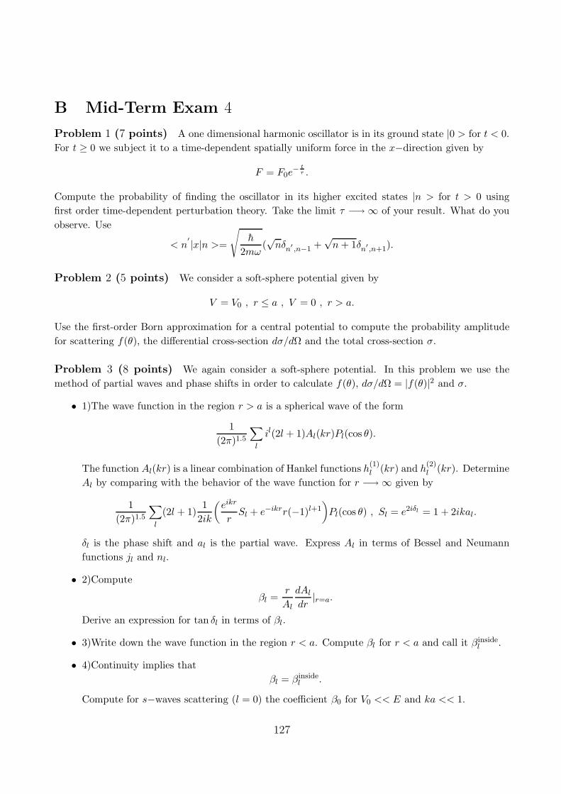
B Mid-Term Exam 4
Problem 1 (7 points) A one dimensional harmonic oscillator is in its ground state |0 > for t < 0.
For t ≥ 0 we subject it to a time-dependent spatially uniform force in the x−direction given by
F = F0e− t
τ .
Compute the probability of finding the oscillator in its higher excited states |n > for t > 0 using
first order time-dependent perturbation theory. Take the limit τ −→ ∞ of your result. What do you
observe. Use
< n′ |x|n >=
√
h
2mω(√nδn′
,n−1 +√n+ 1δn′
,n+1).
Problem 2 (5 points) We consider a soft-sphere potential given by
V = V0 , r ≤ a , V = 0 , r > a.
Use the first-order Born approximation for a central potential to compute the probability amplitude
for scattering f(θ), the differential cross-section dσ/dΩ and the total cross-section σ.
Problem 3 (8 points) We again consider a soft-sphere potential. In this problem we use the
method of partial waves and phase shifts in order to calculate f(θ), dσ/dΩ = |f(θ)|2 and σ.
• 1)The wave function in the region r > a is a spherical wave of the form
1
(2π)1.5
∑
l
il(2l + 1)Al(kr)Pl(cos θ).
The function Al(kr) is a linear combination of Hankel functions h(1)l (kr) and h
(2)l (kr). Determine
Al by comparing with the behavior of the wave function for r −→ ∞ given by
1
(2π)1.5
∑
l
(2l + 1)1
2ik
(
eikr
rSl + e−ikrr(−1)l+1
)
Pl(cos θ) , Sl = e2iδl = 1 + 2ikal.
δl is the phase shift and al is the partial wave. Express Al in terms of Bessel and Neumann
functions jl and nl.
• 2)Compute
βl =r
Al
dAldr
|r=a.
Derive an expression for tan δl in terms of βl.
• 3)Write down the wave function in the region r < a. Compute βl for r < a and call it βinsidel .
• 4)Continuity implies that
βl = βinsidel .
Compute for s−waves scattering (l = 0) the coefficient β0 for V0 << E and ka << 1.
127
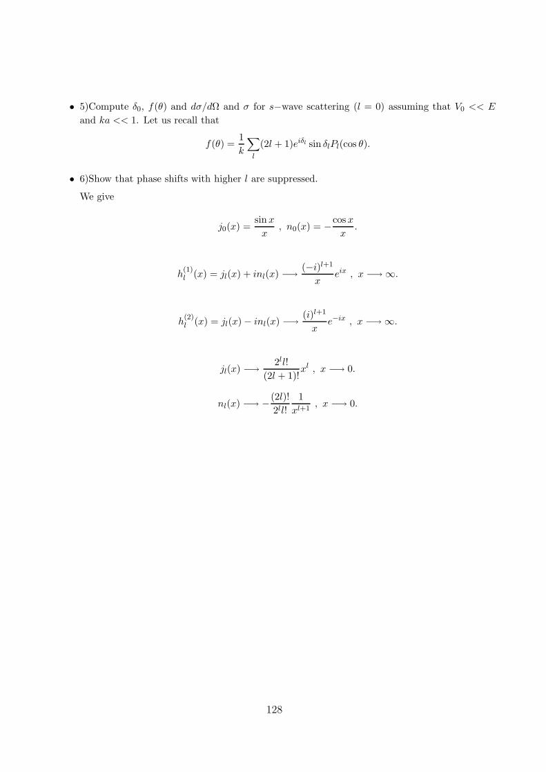
• 5)Compute δ0, f(θ) and dσ/dΩ and σ for s−wave scattering (l = 0) assuming that V0 << E
and ka << 1. Let us recall that
f(θ) =1
k
∑
l
(2l + 1)eiδl sin δlPl(cos θ).
• 6)Show that phase shifts with higher l are suppressed.
We give
j0(x) =sinx
x, n0(x) = −cosx
x.
h(1)l (x) = jl(x) + inl(x) −→
(−i)l+1
xeix , x −→ ∞.
h(2)l (x) = jl(x) − inl(x) −→
(i)l+1
xe−ix , x −→ ∞.
jl(x) −→2ll!
(2l + 1)!xl , x −→ 0.
nl(x) −→ −(2l)!
2ll!
1
xl+1, x −→ 0.
128
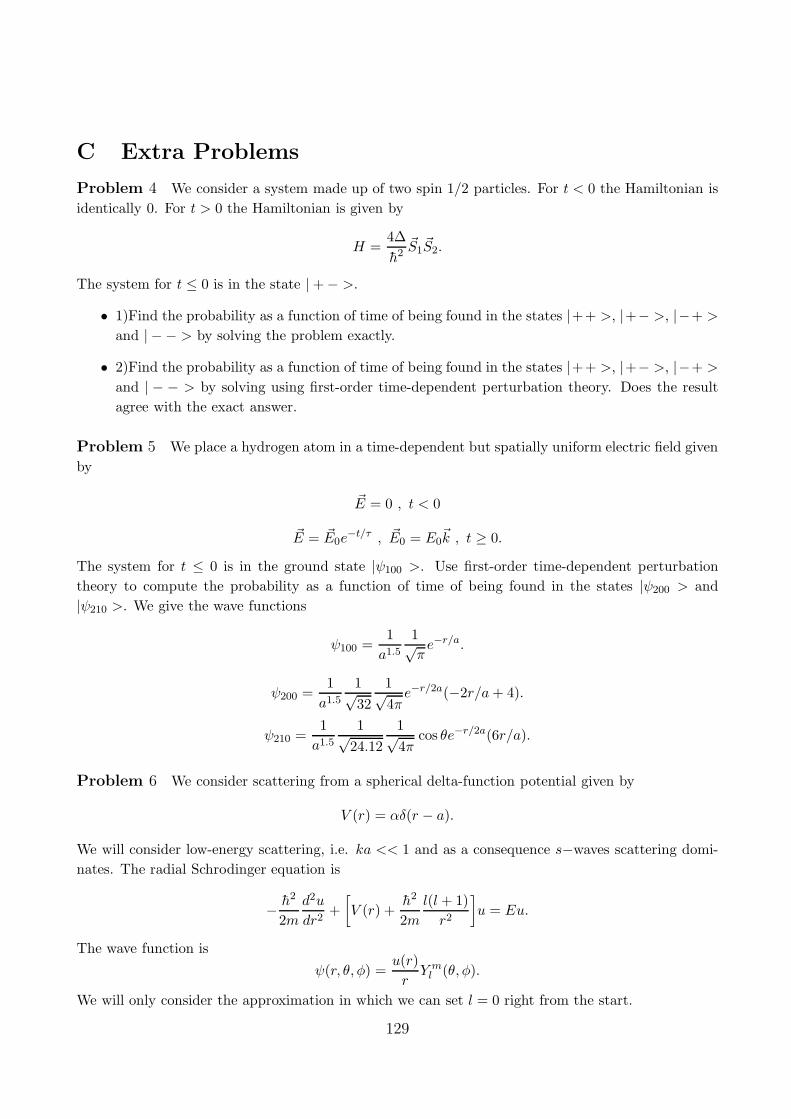
C Extra Problems
Problem 4 We consider a system made up of two spin 1/2 particles. For t < 0 the Hamiltonian is
identically 0. For t > 0 the Hamiltonian is given by
H =4∆
h2~S1~S2.
The system for t ≤ 0 is in the state | + − >.
• 1)Find the probability as a function of time of being found in the states |++ >, |+− >, |−+ >
and | − − > by solving the problem exactly.
• 2)Find the probability as a function of time of being found in the states |++ >, |+− >, |−+ >
and | − − > by solving using first-order time-dependent perturbation theory. Does the result
agree with the exact answer.
Problem 5 We place a hydrogen atom in a time-dependent but spatially uniform electric field given
by
~E = 0 , t < 0
~E = ~E0e−t/τ , ~E0 = E0
~k , t ≥ 0.
The system for t ≤ 0 is in the ground state |ψ100 >. Use first-order time-dependent perturbation
theory to compute the probability as a function of time of being found in the states |ψ200 > and
|ψ210 >. We give the wave functions
ψ100 =1
a1.5
1√πe−r/a.
ψ200 =1
a1.5
1√32
1√4πe−r/2a(−2r/a+ 4).
ψ210 =1
a1.5
1√24.12
1√4π
cos θe−r/2a(6r/a).
Problem 6 We consider scattering from a spherical delta-function potential given by
V (r) = αδ(r − a).
We will consider low-energy scattering, i.e. ka << 1 and as a consequence s−waves scattering domi-
nates. The radial Schrodinger equation is
− h2
2m
d2u
dr2+
[
V (r) +h2
2m
l(l + 1)
r2
]
u = Eu.
The wave function is
ψ(r, θ, φ) =u(r)
rY ml (θ, φ).
We will only consider the approximation in which we can set l = 0 right from the start.
129
• 1)Write down the solution of the radial Schrodinger equation for r < a.
• 2)Write down the general solution for r > a. Compare with the behavior of any spherical
potential for large r which is given by
1
(2π)1.5
∑
l
(2l + 1)1
2ik
(
eikr
rSl + e−ikrr(−1)l+1
)
Pl(cos θ) , Sl = e2iδl = 1 + 2ikal.
Derive an expression for the partial wave a0 in terms of the coefficients of the incoming and
outgoing spherical waves. Write down the wave function in this region in terms of the phase
shift δ0.
• 3)The wave function must be continuous at r = a. Write down the corresponding boundary
condition.
The first derivative of the wave function must be continuous except where the potential diverges.
The corresponding condition reads
∆(du
dr) =
2mα
h2 u(a).
Use these two boundary conditions to determine the partial wave a0.
• 4)Calculate f(θ), dσ/dΩ and σ. What is the answer for ka << 1. Define
β =2maα
h2 .
• 5)Calculate the phase shift δ0.
130
D Examen Final de Mecanique Quantique Avancee
Exercice 1(3 points) We consider the decay of neutral pion: π0 −→ e− + e+. By conservation of
the total angular momentum the electron and positron are in the singlet (entangled) state:
|00 >=1√2(|+ > |− > −|− > |+ >).
We place 2 detectors A and B (Stern-Gerlach magnets) at appropriate locations in order to measure
the component ~S1a of the spin of the electron and the component ~S2b of the spin of the positron where
a and b are unit vectors defined by
a = sin θa cosφai+ sin θa sinφaj + cos θak , b = sin θb cosφbi+ sin θb sinφbj + cos θbk.
Compute the probability
P (a+, b+) = probability of finding ~S1a = +h
2and ~S2b = +
h
2.
Express the answer in terms of the dot product ab.
Exercice 2(4 points)
• 1) We consider the 3−dimensional infinite cubic well:
V (x, y, z) = 0 , if 0 < x < a , 0 < y < a , 0 < z < a
V (x, y, z) = ∞ , otherwise.
Derived the allowed energies and the corresponding wave functions.
Hint:The allowed energies and the corresponding wave functions of the 1−dimensional infinite
square well are
En = En2 , E =π2h2
2ma2.
ψn(x) =
√
2
asin
nπ
ax ,
∫ a
0dx ψ∗
n(x)ψm(x) = δnm.
• 2) We introduce the perturbation:
H1 = V0 , if 0 < x <a
2, 0 < y <
a
2H1 = 0 , otherwise.
Compute the first-order correction to the ground state energy.
• 3)Compute the first-order correction to the first (triply degenerate) excited states.
131
Exercice 3(6 points) We consider a system made up of two spin 1/2 particles. For t < 0 the
Hamiltonian is identically 0. For t > 0 the Hamiltonian is given by
H =4∆
h2~S1~S2.
• 1)Find the probability as a function of time of being found in the states |++ >, |+− >, |−+ >
and | − − > by solving the problem exactly.
• 2)Find the probability as a function of time of being found in the states |++ >, |+− >, |−+ >
and | − − > by solving using first-order time-dependent perturbation theory. The system for
t ≤ 0 is in the state | + − >. Does the result agree with the exact answer.
Exercice 4(7 points) We consider scattering from a spherical delta-function potential given by
V (r) = αδ(r − a).
We will consider low-energy scattering, i.e. ka << 1 and as a consequence s−waves scattering domi-
nates. The radial Schrodinger equation is
− h2
2m
d2u
dr2+
[
V (r) +h2
2m
l(l + 1)
r2
]
u = Eu.
The wave function is
ψ(r, θ, φ) =u(r)
rY ml (θ, φ).
We will only consider the approximation in which we can set l = 0 right from the start.
• 1)Write down the solution of the radial Schrodinger equation for r < a.
• 2)Write down the general solution for r > a. Compare with the behavior of any spherical
potential for large r which is given by
1
(2π)1.5
∑
l
(2l + 1)1
2ik
(
eikr
rSl + e−ikrr(−1)l+1
)
Pl(cos θ) , Sl = e2iδl = 1 + 2ikal.
Derive an expression for the partial wave a0 in terms of the coefficients of the incoming and
outgoing spherical waves. Write down the wave function in this region in terms of the phase
shift δ0.
• 3)The wave function must be continuous at r = a. Write down the corresponding boundary
condition.
The first derivative of the wave function must be continuous except where the potential diverges.
The corresponding condition reads
∆(du
dr) =
2mα
h2 u(a).
Use these two boundary conditions to determine the partial wave a0.
• 4)Calculate f(θ), dσ/dΩ and σ. What is the answer for ka << 1. Define
β =2maα
h2 .
• 5)Calculate the phase shift δ0.
132
E Examen Rattrapage de Mecanique Quantique Avancee
Problem 1 We consider hard sphere scattering given by the potential
V = 0 , r > R
= ∞ , r < R. (887)
Determine the scattering angle, differential cross-section and total cross-section for a classical particle
scattering off the potential V .
Problem 2 We give the Yukawa potential
V (r) = βe−r
r. (888)
Compute the first-order Born amplitude and the differential-cross section. Determine the differential
cross-section for Coulomb scattering. Compare with the classical result of Rutherford.
Problem 3 The energies and wave functions of the one-dimensional infinite square well are given
by
En =n2π2h2
2ma2, ψn(x) =
√
2
asin
nπx
a, n = 1, 2, 3, ... (889)
A time-dependent perturbation is introduced during the time interval T such that the potential be-
comes
V (x) = V0 , 0 ≤ x ≤ a
2
V (x) = 0 ,a
2≤ x ≤ 0
V (x) = ∞ , otherwise. (890)
At t = 0 the system is in the ground state n = 1. What is the probability that at time t = T the
system jumps to the first excited state n = 2.
Problem 4 We place a one-dimensional harmonic oscillator under the influence of a spatially uni-
form time-dependent force given by
F (t) =F0τ
ω(τ2 + t2). (891)
At t = −∞ the harmonic oscillator is in the ground state. Compute the probability that at time
t = +∞ the harmonic oscillator will be found in the first excited state.
133

References
134