the proliferation of centenarians in brazil: indirect ... · marília r. nepomuceno1 cássio m....

The proliferation of centenarians in Brazil:

Indirect estimations using alternative approaches

Marília R. Nepomuceno1

Cássio M. Turra2

Introduction

The proliferation of centenarians is a significant feature of the aging process. In today’s low-

mortality countries, the number of centenarians more than doubled each decade since 1950

(Jeune and Kannisto 1997). On average, the number of new centenarians increased at an

annual rate of about 7% between 1950s and 1980s in these countries (Vaupel and Jeune

1995). In countries with higher mortality, like Brazil, the multiplication of centenarians has

been observed as well. In Brazil, according to census data, there were 13,296 centenarians in

1991 and 24.236 in 2010 (IBGE 1991, 2010). However, due to data quality issues, these

numbers are questionable. Accurate estimates of the number of the oldest-old population are

important for correctly assessing the current scale of the aging process and predicting future

demographic and socioeconomic changes.

In any population, the growth rate of centenarian population must be due to some combination

of earlier changes in fertility, migration and mortality (Preston and Coale 1982). According to

Vaupel and Jeune (1995), improvements in survival from age 80 to 100 is the main cause of

the proliferation of centenarians, explaining about 70% of the growth rate of centenarian

population in Northern and Western-central Europe from the 1970s to 1980s. The case of

Japan is a good example of this aspect. Japanese population experienced high rates of

mortality improvement for ages 80-99 from 1960s to the 1980s (Kannisto et al. 1994), which

probably triggered the increased number of centenarians from 153 people in 1963 to 40,399

people in 2009 (Saito 2005, Robine et al. 2010). In Brazil, average death rates of

octogenarians have declined at a rate of 2.9% per year for males and 3.5% per year for

females in the 1980s (Campos 2004). Indirect estimates of mortality rates also suggested

mortality reduction at ages above 80 in the period 1980 to 2000 (Agostinho 2009). Mostly of

this mortality decline is a result of economic developments, investments in public health and

advances in medical technology. Moreover, improvements in survival at older ages over the

past decades certainly contributed to the proliferation of centenarians in Brazil.

Trabalho apresentado no VII Congreso de la Asociación LatinoAmericana de Población e XX Encontro

Nacional de Estudos Populacionais, realizado em Foz do Iguaçu/PR – Brasil, de 17 a 22 de outubro de 2016.

1 Ph.D Student, Department of Demography – Cedeplar, Universidade Federal de Minas Gerais, Brazil.

2 Associate Professor, Department of Demography – Cedeplar, Universidade Federal de Minas Gerais, Brazil.

A simple comparison between the Brazilian proportions of centenarians over the years makes

us skeptical about the population counts reported by the census bureau, suggesting variations

in data quality across censuses. According to census data, the centenarian share of the total

population was 0.91 per 10,000 in 1991, 1.45 per 10,000 in 2000 and 1.27 per 10,000 in 2010

(IBGE 1991, 2000, 2010). Due to declining mortality at older ages over decades, we expected

an increasing proportion of centenarians in Brazil. Probably, the decline in proportion of

centenarians between 2000 and 2010 is a result of progress in census data quality, such as

improvements in age reported caused by higher education at advanced ages.

Another simple way to check the quality of the Brazilian centenarian data is comparing the

prevalence of centenarians in Brazil with a country with presumably higher data quality and

lower mortality levels. In Sweden, for instance, the centenarian share of the total population in

1991 (0.69 per 10.000) was about 2/3 the Brazilian proportion in 1991 (HMD 2016).

Conversely, the Swedish proportion of centenarians in 2010 (1.72 per 10.000) is 35% higher

than that of Brazil in 2010 (HMD 2016). This improbably higher proportion of older

population in the 1991 census in Brazil could be a result of the poor quality data. However,

the comparison in 2010 suggests census data improvements in Brazil.

Official population estimates are especially problematic at advanced ages. Therefore, studies

of the centenarian population must take into account data quality issues. In many populations,

the most important problem of census data at older ages is age misstatement (Preston et al.

1999). In Brazil, the age reporting in the 1991, 2000 and 2010 census is derived from two

questions. The first one asked the month and year of birth of the person. The second question

asked for the presumably age in years and months and is used when the person do not know

her date of birth. In the absent of these two answers, information of age is imputed by the

census bureau. Using the presumably age, the error of digit preference can emerge. Brazilians

tend to prefer the ending age digits zero and five (Horta 2012; Horta, Sawyer e Carvalho

2006). Both problems of digit preference and of missing data are very significant among the

oldest-old population (Popolo 2001, Gomes and Turra 2009). The problem of age

exaggeration is also common at advanced ages (Popolo 2001, Dechter and Preston 1991). All

the problems mentioned above are believed to be responsible for an overstatement of the

number of centenarians in Brazil. Moreover, the relatively small number of centenarians in a

population can cause data to be particularly sensitive to these data issues.

The poor data quality at advanced ages increases the uncertainty of the true number of

centenarians recorded in the Brazilian census bureau. Therefore, indirect methods are very

helpful to evaluate the quality of census data, and to estimate the number of centenarians

closer to the true size of the oldest-old population. In Brazil, indirect estimates based on the

extinct generation method revealed that the centenarians recorded in the 1991 census are

exaggerated (Gomes and Turra 2009). This study suggested that the number of centenarians

estimated indirectly is one third the number recorded by the 1991 census in Brazil.

Nevertheless, few studies have analyzed centenarians in Brazil. Indeed, little is known about

the true proliferation of centenarians in Brazil during the last decades.

In order to complement analysis of centenarians in Brazil, we estimate the population aged

100 to 109 years by sex in 1991, 2000 and 2010 using three estimation procedures. First we

use a method developed by Wilmoth (1995) to compute the proportion of centenarians in a

stable population. The second estimation procedure is a variant of Wilmoths’ method. Instead

of assume a stable population, we compute the proportion of centenarians in a non-stable

population, considering a set of age-specific growth rates. Finally, we estimate the centenarian

population “projecting” the population at one census date to a later date using the forward-

survival method (Shryock and Siegel 1976).

Methods and Data

In this study we estimate the number of people at age group 100-109 by sex, for 1991, 2000

and 2010. To do that, three estimation procedures are used: (i) the Wilmoth’s method

assuming a stable population; (ii) the Wilmoth’s method assuming a non-stable population;

and (iii) the cohort reconstruction through the forward-survival method.

i. First estimation procedure

First, we use the indirect method develop by Wilmoth (1995). This method computes the

proportion of centenarian using a mortality model to estimate the survival probability from a

given adult age y to 100.

The first step of the Wilmoths’ method is to choose an age pattern of mortality to estimate the

survival probability from a given adult age y to age 100. There is a general agreement that

mortality increases exponentially, as described by the Gompertz curve, for mid-adult and

early old ages. However, there is not a consensus regarding the mortality trajectory at the

most advanced ages (Gavrilov and Gavrilova 2015; Gavrilov and Gavrilova 2011; Gampe

2010; Robine et al. 2005; Robine and Vaupel 2001). Some studies suggested that the

exponential growth of mortality with age is followed by a period of deceleration, with slower

rates of mortality increase at the oldest ages (Gampe 2010; Robine and Vaupel 2001; Robine

et al. 2005). Conversely, another group of researchers pointed out that the mortality

deceleration in later life is more expressed for data with lower quality, and hence mortality

continues to grow exponentially at the highest ages (Gavirilov and Gavirilova 2011, 2015).

Due to this disagreement about the mortality trajectory at the most advanced ages, we decide

to assume that mortality slows down at the most advanced ages, as assumed by Wilmoth

(1995). Moreover, we assume that the age 50 (y=50) is the starting point for our model of

adult mortality. This choice can be justified by the importance of adult mortality in

centenarians’ mortality (Vaupel and Jeune 1995).

The Gompertz-Perks curve follows a logistic form, and it is a modification of the well-known

Gompertz mortality curve. The Gompertz-Perks curve deviates from the Gompertz model at

both younger and older adult ages, and it contains an inflection point in late adulthood that

should move upward as mortality falls. The Gompertz-Perks formula contains 4 parameters:

( )1

bx

bx

c aex

vae

(1)

where 0c represents the level of background mortality, and 1/ v gives the upper asymptote

of the mortality curve. The parameters a and b are more abstract, where 0b is the rate of

exponential increase in mortality across the age range in the Gompertz model, but this

interpretation is only approximate in the Gompertz-Perks model (Wilmoth 1995), and 0a is

the exact force of mortality at age 0 only in the Gompertz model, but this fact does not aid in

interpretation since the model applies to adult mortality alone (Wilmoth 1995).

To lend these parameters more direct interpretations, Wilmoth (1995) proposed a re-

parametrization of the Gompertz-Perks model. According to the author, the remaining life

expectancy at the starting age for the late adult mortality model, 50e , is an alternative for the

parameter a, and the death rate between ages 50 and 55 ( 5 50m ) is chosen as alternative for the

parameter b in the formula (1). Using numerical methods3 we find the unique parameters, a

and b, in the formula (1) that reproduce a given 50e and 5 50m . Thus, all model assumptions in

this study are expressed in terms of 50e , 5 50m , c and v.

a) Choosing the mortality levels for 1991, 2000 and 2010

Having chosen the mortality curve, it is necessary to select the parameters of the Gompertz-

Perks model. We start selecting the mortality levels: (1) life expectancy at birth ( 0e ), and (2)

3 We used numerical optimization to find the maximum likelihood estimate of the parameter a given b

using the equation (1) and assuming that 5 50(52.5) m .

the remaining life expectancy at age 50 ( 50e ). To select these values we use a combination of

sources in order to calculate the average of 0e and 50e . We believe to achieve more accurate

values of 0e and 50e through a combination of sources.

We use the life expectancy at birth as a reference measure to select life tables of countries

with better data quality than Brazil. To define the 0e for 1991, 2000 and 2010 in Brazil, we

use Brazilian life tables estimated by: (a) the Brazilian Institute of Geography and Statistics

(IBGE) for 1991, 2000 and 2010, (b) Agostinho (2009) for 1991 and 2000, (c) the World

Health Organization for 1990 and 2000, (d) and by the Centre for Development and Regional

Planning (CEDEPLAR) for 2010. The average life expectancy at birth based on these sources

is: 70.4 years for female and 63.6 years for male in 1991, 74.0 years for female and 67.0 years

for male in 2000, and 77.2 years for female and 70.3 for male in 2010. Thus, we consider

these values as more accurate estimates of life expectancy at birth in Brazil.

After define 0e , we choose 50e (parameter a) for 1991, 2000 and 2010 in Brazil. Instead of use

only Brazilian life tables we also use life tables from several countries with presumably

higher quality data4 than Brazil to calculate the average of 50e . The life expectancy at birth

defined to Brazil, are our reference measure to select life tables of low-mortality countries.

For instance, the female 0e in 2010 in Brazil (77.2 years) it is close to the female 0e in 1970

in Sweden (77.2 years). Thus, the Swedish life table for females in 1970 is used to determine

the 50e in 2010 for females in Brazil. Thus, the average of 50e from the selected life tables is

believed to be a more accurate estimate than the 50e based on only Brazilian life tables. Our

strategy here is to reduce the effects of data quality issues on mortality rates at older ages in

Brazil5.

Tables 1 and 2 present the values of 0e and 50e used to define the remaining life expectancy

at age 50 in 1991, 2000 and 2010 in Brazil, respectively for females and males.

From these results, we assume that the remaining life expectancy at age 50 in 1991, 2000, and

2010 in Brazil are the average of 50e derived from the selected life tables (Tables 1 and 2).

Thus, the 50e is around 26 years for females and 22 years for males in 1991, around 27 years

4 We selected life tables of today’s low-mortality countries with 0e in the range:

0 0 0 0 0( ) ( ) ( ) ( )Brazil Brazil low mortality countries Brazil Brazilmean e standard deviation e e mean e standard deviation e 5 Number of deaths is not recorded quite precisely in Brazil. Moreover, age misreporting also affects

census data, especially at older ages.

for females and 23 years for males in 2000, and around 30 years for females and 24 for males

in 2010.

Table 1: Life expectancies at birth ( 0e ) and at age 50 ( 50e ) and proportion of surviving at age

50 (l(50)) in the selected low-mortality countries and Brazil, female.

Country

Reference year to estimate the centenarians in Brazil

1991 2000 2010

Year e0 e50 l(50) Year e0 e50 l(50) Yearr e0 e50 l(50)

Brazil 1991 70.5 26.3 0.8917 2000 74.0 27.7 0.9298 2010 77.3 29.9 0.9513

Sweden 1945 69.5 26.1 0.8717 1954 73.9 27.2 0.9330 1970 77.2 29.8 0.9496

Sweden 1946 70.7 26.2 0.8906 1955 74.2 27.6 0.9333 1971 77.4 29.9 0.9501

Sweden 1947 70.6 25.9 0.8932 - - - - 1972 77.5 30.0 0.9523

Italy 1954 69.9 27.0 0.8799 1968 73.7 28.1 0.9225 1978 77.1 29.9 0.9501

Italy 1955 70.4 27.1 0.8853 1969 73.9 28.2 0.9225 1979 77.5 30.1 0.9516

Italy 1956 69.8 26.2 0.8886 1970 74.9 28.9 0.9225 1981 77.8 30.2 0.9542

Italy 1957 70.1 26.8 0.8861 1971 73.7 27.4 0.9225 - - - -

Italy 1958 71.2 27.5 0.8937 - - - - - - - -

Japan 1959 69.8 26.2 0.8788 1966 73.7 27.4 0.9258 1977 77.9 30.2 0.95487

Japan 1960 70.2 26.0 0.8873 1967 74.0 27.6 0.9281 - - - -

Japan 1961 70.8 26.2 0.8960 1968 74.3 27.7 0.9320 - - - -

Japan 1962 71.1 26.2 0.9021 1969 74.6 27.9 0.9335 - - - -

Switzerland 1948 69.4 25.5 0.8827 1958 73.9 27.6 0.9306 1974 77.6 30.1 0.95229

Switzerland 1949 70.0 25.6 0.8933 - - - - - - - -

Switzerland 1950 71.1 26.2 0.9015 - - - - - - - -

Switzerland 1951 71.0 26.0 0.9020 - - - - - - - -

Portugal 1968 69.9 27.4 0.8781 1977 73.9 28.4 0.9195 1986 77.1 30.2 0.9431

Portugal 1970 70.1 27.5 0.8804 - - - - - - - -

UK 1949 70.3 26.1 0.8879 1963 73.7 27.3 0.9290 1983 77.2 29.5 0.95472

UK 1950 70.9 26.2 0.8972 - - - - 1984 77.6 29.8 0.95604

UK 1951 70.7 25.7 0.9011 - - - -

Finland 1955 70.7 25.5 0.9041 1970 74.4 27.2 0.9426 - - - -

Finland 1956 71.2 25.8 0.9072 - - - - - - - -

Finland 1957 70.6 25.5 0.9036 - - - - - - - -

Denmark 1947 69.6 25.7 0.8822 1956 73.7 27.5 0.9271 - - - -

Denmark - - - - 1957 73.5 27.3 0.9261 - - - -

Denmark - - - - 1958 74.0 27.5 0.9321 - - - -

Denmark - - - - 1959 73.9 27.6 0.9287 - - - -

Denmark - - - - 1960 74.0 27.5 0.9316 - - - -

Denmark - - - - 1961 74.4 28.0 0.9312 - - - -

Denmark - - - - 1962 74.4 27.8 0.9344 - - - -

Belgium 1952 70.5 26.4 0.8932 1965 73.6 27.5 0.9265 1982 77.2 29.7 0.94933

Belgium 1953 70.9 26.4 0.9000 1966 73.7 27.5 0.9263 1983 77.2 29.7 0.94857

Belgium 1954 71.1 26.6 0.9006 1967 74.1 27.7 0.9304 1984 77.8 30.2 0.95174

Belgium - - - - 1968 73.8 27.3 0.9324 - - - -

Belgium - - - - 1969 74.0 27.5 0.9312 - - - -

Belgium - - - - 1970 74.2 27.7 0.9315 - - - -

Belgium - - - - 1971 74.4 27.8 0.9340 - - - -

Source: HMD data.

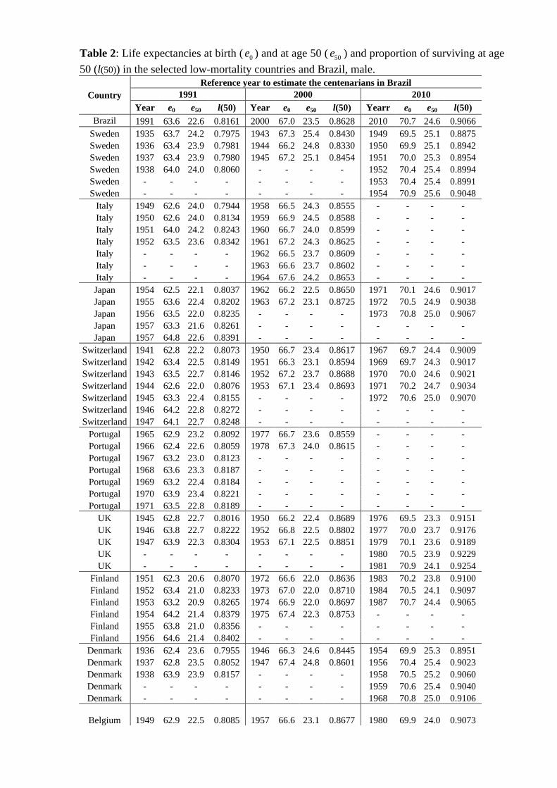
Table 2: Life expectancies at birth ( 0e ) and at age 50 ( 50e ) and proportion of surviving at age

50 (l(50)) in the selected low-mortality countries and Brazil, male.

Country

Reference year to estimate the centenarians in Brazil

1991 2000 2010

Year e0 e50 l(50) Year e0 e50 l(50) Yearr e0 e50 l(50)

Brazil 1991 63.6 22.6 0.8161 2000 67.0 23.5 0.8628 2010 70.7 24.6 0.9066

Sweden 1935 63.7 24.2 0.7975 1943 67.3 25.4 0.8430 1949 69.5 25.1 0.8875

Sweden 1936 63.4 23.9 0.7981 1944 66.2 24.8 0.8330 1950 69.9 25.1 0.8942

Sweden 1937 63.4 23.9 0.7980 1945 67.2 25.1 0.8454 1951 70.0 25.3 0.8954

Sweden 1938 64.0 24.0 0.8060 - - - - 1952 70.4 25.4 0.8994

Sweden - - - - - - - - 1953 70.4 25.4 0.8991

Sweden - - - - - - - - 1954 70.9 25.6 0.9048

Italy 1949 62.6 24.0 0.7944 1958 66.5 24.3 0.8555 - - - -

Italy 1950 62.6 24.0 0.8134 1959 66.9 24.5 0.8588 - - - -

Italy 1951 64.0 24.2 0.8243 1960 66.7 24.0 0.8599 - - - -

Italy 1952 63.5 23.6 0.8342 1961 67.2 24.3 0.8625 - - - -

Italy - - - - 1962 66.5 23.7 0.8609 - - - -

Italy - - - - 1963 66.6 23.7 0.8602 - - - -

Italy - - - - 1964 67.6 24.2 0.8653 - - - -

Japan 1954 62.5 22.1 0.8037 1962 66.2 22.5 0.8650 1971 70.1 24.6 0.9017

Japan 1955 63.6 22.4 0.8202 1963 67.2 23.1 0.8725 1972 70.5 24.9 0.9038

Japan 1956 63.5 22.0 0.8235 - - - - 1973 70.8 25.0 0.9067

Japan 1957 63.3 21.6 0.8261 - - - - - - - -

Japan 1957 64.8 22.6 0.8391 - - - - - - - -

Switzerland 1941 62.8 22.2 0.8073 1950 66.7 23.4 0.8617 1967 69.7 24.4 0.9009

Switzerland 1942 63.4 22.5 0.8149 1951 66.3 23.1 0.8594 1969 69.7 24.3 0.9017

Switzerland 1943 63.5 22.7 0.8146 1952 67.2 23.7 0.8688 1970 70.0 24.6 0.9021

Switzerland 1944 62.6 22.0 0.8076 1953 67.1 23.4 0.8693 1971 70.2 24.7 0.9034

Switzerland 1945 63.3 22.4 0.8155 - - - - 1972 70.6 25.0 0.9070

Switzerland 1946 64.2 22.8 0.8272 - - - - - - - -

Switzerland 1947 64.1 22.7 0.8248 - - - - - - - -

Portugal 1965 62.9 23.2 0.8092 1977 66.7 23.6 0.8559 - - - -

Portugal 1966 62.4 22.6 0.8059 1978 67.3 24.0 0.8615 - - - -

Portugal 1967 63.2 23.0 0.8123 - - - - - - - -

Portugal 1968 63.6 23.3 0.8187 - - - - - - - -

Portugal 1969 63.2 22.4 0.8184 - - - - - - - -

Portugal 1970 63.9 23.4 0.8221 - - - - - - - -

Portugal 1971 63.5 22.8 0.8189 - - - - - - - -

UK 1945 62.8 22.7 0.8016 1950 66.2 22.4 0.8689 1976 69.5 23.3 0.9151

UK 1946 63.8 22.7 0.8222 1952 66.8 22.5 0.8802 1977 70.0 23.7 0.9176

UK 1947 63.9 22.3 0.8304 1953 67.1 22.5 0.8851 1979 70.1 23.6 0.9189

UK - - - - - - - - 1980 70.5 23.9 0.9229

UK - - - - - - - - 1981 70.9 24.1 0.9254

Finland 1951 62.3 20.6 0.8070 1972 66.6 22.0 0.8636 1983 70.2 23.8 0.9100

Finland 1952 63.4 21.0 0.8233 1973 67.0 22.0 0.8710 1984 70.5 24.1 0.9097

Finland 1953 63.2 20.9 0.8265 1974 66.9 22.0 0.8697 1987 70.7 24.4 0.9065

Finland 1954 64.2 21.4 0.8379 1975 67.4 22.3 0.8753 - - - -

Finland 1955 63.8 21.0 0.8356 - - - - - - - -

Finland 1956 64.6 21.4 0.8402 - - - - - - - -

Denmark 1936 62.4 23.6 0.7955 1946 66.3 24.6 0.8445 1954 69.9 25.3 0.8951

Denmark 1937 62.8 23.5 0.8052 1947 67.4 24.8 0.8601 1956 70.4 25.4 0.9023

Denmark 1938 63.9 23.9 0.8157 - - - - 1958 70.5 25.2 0.9060

Denmark - - - - - - - - 1959 70.6 25.4 0.9040

Denmark - - - - - - - - 1968 70.8 25.0 0.9106

Belgium

1949

62.9

22.5

0.8085

1957

66.6

23.1

0.8677

1980

69.9

24.0

0.9073

Belgium - - - - 1958 67.3 23.3 0.8768 1981 70.3 24.2 0.9106

Belgium - - - - - - - - 1982 70.6 24.4 0.9145

Belgium - - - - - - - - 1983 70.6 24.4 0.9129

Belgium - - - - - - - - 1984 71.0 24.7 0.9156

Source: HMD data.

b) Choosing the mortality pattern for 1991, 2000 and 2010

Aside from the question of mortality levels, it is also necessary to make assumptions about the

relationships that determine the age pattern of mortality in Brazil. In the Gompertz-Perks

model, the mortality curve is fully specified only when a chosen value of 50e is accompanied

by assumptions regarding 5 50m , c and v. The parameters 50e , 5 50m and c tend to be strongly

correlated, so they must be chosen in a manner to insure that the resulting mortality curve is

plausible. Therefore, the relationships between these parameters are expressed here by a series

of regression, based on life tables indicated on Tables 1 and 2.

In the first regression we choose 5 50m for a given level of 50e . Figures 1 and 2 present the

inverse log-linear relationship that is typical for 50e and 5 50m , for females and males

respectively in 1991, 2000 and 2010. These figures also show the regression line. In the

analyses that follow, the choice of 5 50m for a given 50e is centered on the value given by these

regression lines. The regressions of 5 50log( )m on 50e for females explain 76% of the variance

in 5 50log( )m in 1991, 71% in 2000 and 84% in 2010. For males these percentage are 86%,

84% and 81% for 1991, 2000 and 2010, respectively. Tables 1A and 2A in the Appendix

present the results of all regressions to predict 5 50log( )m (Model 1) in 1991, 2000 and 2010,

for females and males respectively.

Figure 1 – Relationship between 50e and 5 50m , females, 1991, 2000, 2010.

Note: The dashed line corresponds to the regression line.

Source: authors’ own calculation based on HMD data.

Figure 2 – Relationship between 50e and 5 50m , males, 1991, 2000, 2010.

Note: The dashed line corresponds to the regression line.

Source: authors’ own calculation based on HMD data.

The method for choosing values of the background mortality parameter, c, involves a multiple

regression. Figures 3 and 4 present the strong relationship between c and 50e in 1991, 2000

and 2010, for females and males respectively. For all years analyzed the Spearman’s

correlation coefficient are negative and higher than 0.70 for females, and higher than 0.78

males.

Figure 3 - Relationship between 50e and

c, females, 1991, 2000, 2010.

Source: authors’ own calculation based on HMD

2016.

Figure 4 - Relationship between 50e and

c, males, 1991, 2000, 2010.


2016.

The relationship between c and 5 50m are presented in Figures 5 and 6. A strong relationship is

also observed between 5 50m and c. The Spearman’s correlation coefficient is 0.89 for females

and 0.91 for males in 1991, 0.71 for females and 0.89 for males in 2000, and 0.85 for females

and 0.86 for males in 2010.

For males in all analyzed years, the best prediction is achieved by regressing c on both 50e

and 5 50m (Table 2A-Model 2). For females in 1991 and 2000, the best regression is between c

and 5 50m , while for 2010 the best regression is achieved between c and 50e (Table 1A-Model

2). The criteria use to select the best regressions are the t-student test to check the significance

of coefficients, and the coefficient of determination ( 2R ), which measures the variability in

the data explained by the regression model.

Figure 5 - Relationship between 5 50m and

c, females, 1991, 2000, 2010.


2016.

Figure 6 - Relationship between 5 50m and

c, males, 1991, 2000, 2010.


2016.

The last parameter to be chosen is v. It determines the upper asymptote of the mortality curve.

Unlike the other parameters, the parameter v is chosen in a more arbitrary fashion, based on

empirical evidence about typical value of this parameter. Robine et al. (2005) and Gampe

(2010) revealed that the human mortality after age 110 is flat at a constant level of 0.7 in

today’s low mortality countries, corresponding an annual probability of death of 0.5. Since

higher values of v are associated with lower mortality rates at high ages (Wilmoth 1995), we

assume a lower value of v than that of the low-mortality countries. Thus, we consider in this

study 0.6v .

In addition to choose the four parameters of the Gompertz-Perks curve, the proportion

surviving from birth to age 50 ( (50)l ) is needed to estimate the prevalence of centenarians.

First we tried to choose (50)l using multiple regression of (50)l against 50e , 5 50m and c.

However, these regression were not satisfactory, explaining less than 30% of the variance in

(50)l , for both female and male. Therefore, we use the same strategy as that to choose the 50e .

We assume that the proportion surviving from birth to age 50 in Brazil is the average of (50)l

derived from the listed life tables in Tables 1 and 2, respectively for females and males.

From these results, we define that (50)l is: 0.8917 for female and 0.8161 for male in 1991,

0.9298 for female and 0.8628 for male in 2000, and 0.9516 for female and 0.9066 for male in

2010.

Having chosen all parameters of the Gompertz-Perks curve, we can calculate the probability

of survival from age 50 to 100:

1 1

( )

1 0( )

1( )

0bx by

cbx b v

c x y

by

ac x y e e

b

vaee if vl x

vael y

e if v

(2)

where x = 100 and y =50.

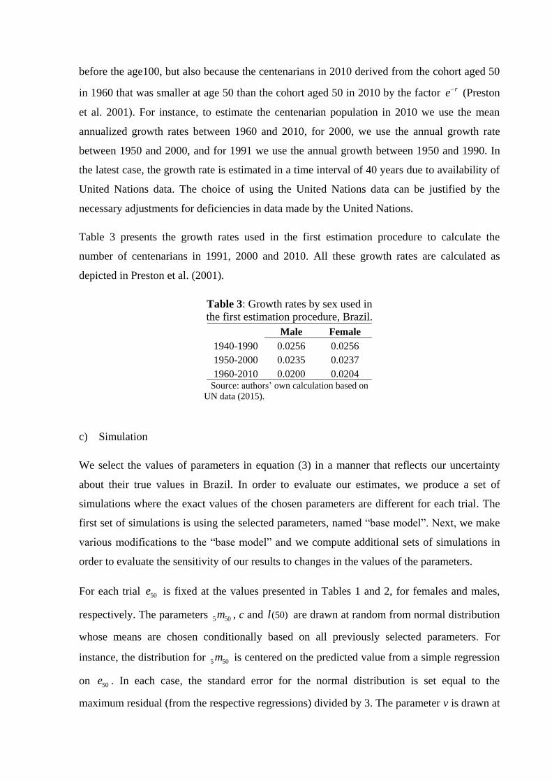
In this first estimation procedure, we estimate the prevalence of centenarians in a stable

population as follows:

100

100

100

0

100

0

100

0

( )

( )

=

( )

( )

( ) ( )

( )( )

( )

( )( ) ( )

( )

rx

rx

rx

rx

y

rx rx

y

rx

y

rx rx

y

c be l x dx

e l x dx

e l x dx

e l x dx

e l x dx e l x dx

l xl y e dx

l y

l xe l x dx l y e dx

l y

(3)

where x in these integrals denotes age, b (only in this equation (3)) is the birth rate, is the

latest attained age (110 in this study), r is the constant population growth rate, ( )xl is the

probability of survival from age 0 to x, and y is the age 50.

The idea of the growth rate in formula (3) is to adjust the size of the cohort aged 50 with the

size of cohort aged 100 at the same period. For instance, in 2010, the number of centenarians

is smaller than the number of 50-years old people not only because some 50-years old died

before the age100, but also because the centenarians in 2010 derived from the cohort aged 50

in 1960 that was smaller at age 50 than the cohort aged 50 in 2010 by the factor re (Preston

et al. 2001). For instance, to estimate the centenarian population in 2010 we use the mean

annualized growth rates between 1960 and 2010, for 2000, we use the annual growth rate

between 1950 and 2000, and for 1991 we use the annual growth between 1950 and 1990. In

the latest case, the growth rate is estimated in a time interval of 40 years due to availability of

United Nations data. The choice of using the United Nations data can be justified by the

necessary adjustments for deficiencies in data made by the United Nations.

Table 3 presents the growth rates used in the first estimation procedure to calculate the

number of centenarians in 1991, 2000 and 2010. All these growth rates are calculated as

depicted in Preston et al. (2001).

Table 3: Growth rates by sex used in

the first estimation procedure, Brazil.

Male Female

1940-1990 0.0256 0.0256

1950-2000 0.0235 0.0237

1960-2010 0.0200 0.0204 Source: authors’ own calculation based on

UN data (2015).

c) Simulation

We select the values of parameters in equation (3) in a manner that reflects our uncertainty

about their true values in Brazil. In order to evaluate our estimates, we produce a set of

simulations where the exact values of the chosen parameters are different for each trial. The

first set of simulations is using the selected parameters, named “base model”. Next, we make

various modifications to the “base model” and we compute additional sets of simulations in

order to evaluate the sensitivity of our results to changes in the values of the parameters.

For each trial 50e is fixed at the values presented in Tables 1 and 2, for females and males,

respectively. The parameters 5 50m , c and (50)l are drawn at random from normal distribution

whose means are chosen conditionally based on all previously selected parameters. For

instance, the distribution for 5 50m is centered on the predicted value from a simple regression

on 50e . In each case, the standard error for the normal distribution is set equal to the

maximum residual (from the respective regressions) divided by 3. The parameter v is drawn at

random from a normal distribution centered on 0.6, with a standard error of 0.2. The

population growth rates are fixed at the values presented in Table 3.

After choosing the parameters for each simulation trial, the equation (3) is used to compute

the prevalence of centenarians, expressed as a proportion of the total stable population.

ii. Second estimation procedure

The second estimation procedure also considers the Gompertz-Perks curve with the same

parameters defined for the first procedure. However, unlike the first estimation procedure, this

procedure estimates the prevalence of centenarians in a non-stable population, assuming a set

of age-specific growth rates as follows:

1

3 2

* 100100

0

( )( )

( )

( )( ) ( )

( )

r x

y

r xr x

y

l xl y e dx

l yc

l xe l x dx l y e dx

l y

(4)

where 1r is the growth rate of population age 100 years or over, 2r is the growth rate at ages 0

to 50, and 3r is the growth rate of population age 50 years or over. Due to quality issues in

centenarian data, as already mentioned, we assume that 1r is the growth rate of population age

50 years or over.

As in the first procedure, to estimate the number of centenarians in 2010, we use the annual

growth rates between 1960 and 2010. For 2000 we use the annual growth rates between 1950

and 2000, and for 1991 the annual growth rates between 1950 and 1990. Table 4 presents the

set of age-specific annual growth rates using in the second.

Table 4: Age-specific growth rates by sex used in the second estimation procedure, Brazil.

Source: authors’ own calculation based on UN data (2015).

It is relevant to mention that we use here the same simulation process describe in the first

estimation procedure.

1950-1990 1950-2000 1960-2010 1950-1990 1950-2000 1960-2010

r 1 (50+) 0.0300 0.0302 0.0318 0.0297 0.0303 0.0322

r 2 (0-50) 0.0251 0.0226 0.0181 0.0250 0.0226 0.0181

r 3 = r 1 0.0300 0.0302 0.0318 0.0297 0.0303 0.0322

Male Female

iii. Third estimation procedure

The third estimation procedure involves a reconstruction of two cohorts at the same census

(one initial cohort aged 50-54 years and the other cohort aged 55-59), advancing these cohorts

through successive 5-year time intervals. To do that, we apply the forward-survival method,

“projecting” the population at one census date to a later date through the use of appropriate

survival probabilities. The accuracy of estimates using this approach depends upon the

accuracy of the initial population and the survival rates. In addition, we assume that net

immigration equaled or approximated zero. The initial population is the population at age

groups 50-54 and 55-59 recorded in the 1940, 1950 and 1960 Brazilian census. The data

quality issues common in centenarian data, like age exaggeration, are presumably somewhat

more accurate at these younger ages, at least in terms of 5-years age groups. On the other

hand, some error in the survival rates, like under-registration of deaths, can overestimate our

centenarian population. On balance, the projected number of centenarians in 1990, 2000 and

2010 based on the 1940, 1950 and 1960 census, respectively, are believed to be a more

accurate estimate and less likely to be an overstatement than the number of centenarians direct

report in census.

Applying survival probabilities (in quinquennial age groups by sex) to the census population

aged 50-54 and 55-59 yields an estimate of the number of individuals aged 100-104 and 105-

109 years, respectively.

The equations used to reconstruct the cohort aged 50-54 at one census date until the age group

100-104 50 years later are:

5

5 55 5 50 5 50

10 5 5

5 60 5 55 5 55

50 45 45

5 100 5 95 5 95

i i i

i i i

i i i

N N p

N N p

N N p

(5)

where i is the initial census year, 5 50

iN is the initial cohort at age group 50-54 at year i,

5

5 55

iN is the estimated number of individuals at age group 55-59 at year i+5, and so on; 5 50

ip

is the probability of surviving from age 50 to 54 at year i, 5

5 55

ip is the probability of

surviving from age 55 to 59 at year i+5, and so on.

For the cohort aged 55-59 at one census date until the age group 105-109 the equations are:

5

5 60 5 55 5 55

10 5 5

5 65 5 60 5 60

50 45 45

5 105 5 100 5 100

i i i

i i i

i i i

N N p

N N p

N N p

(6)

Through the equations (5) and (6) we achieve the number of individuals at age groups 100-

104 and 105-109, respectively for 1991, 2000 and 2010 in Brazil.

The choice of life tables from which the survival rates are computed is crucial to this

estimation procedure. Therefore, we use the Brazilian abridged life tables for males and

females, calculated by the United Nations from 1950-1955 to 2010-2015 (UN 2015). The

United Nations made the necessary adjustments for deficiencies in age reporting, under-

enumeration, or underreporting of vital events. The open-ended age interval of these life

tables begins with age 85, thus, in order to estimate death rates until the age 110, we fit the

Kannisto model of old age mortality to distribute deaths in the open-ended age interval

(Thatcher et al. 1998). The Kannisto model has the following form:

0

0

( )

( )( )

1

b x x

b x x

aex

ae

(6)

where 0 85 20x , and a and b are unknown parameters estimated through the optimization

of the equation (6).

Tables 6 and 7 show the age-specific survival probabilities for female and male, respectively,

used to cohort reconstruction. Due to the availability of survival probabilities only from 1950-

1955, we assume that the survival probabilities at age groups 50-54, 55-59 and 60-64 for the

periods 1940-1945 and 1945-1950 are equal to the survival probabilities at the same age

groups for the period 1950-1955. The size of initial cohorts by sex a presented in Table 8.

Table 6 – Survival probabilities by 5-year age group, female, Brazil, 1950-1955 to 2005-2010.


Table 7 – Survival probabilities by 5-year age group, male, Brazil, 1950-1955 to 2005-2010.


Table 8 – Initial cohorts at age groups 50-54 and

55-59 by sex, Brazil

Year Age group 50-54 Age group 55-59

Female Male Female Male

1940 549,886 590,975 441,568 462,478

1950 715,320 763,270 574,414 597,310

1960 1,017,706 1,094,744 817,234 856,710

Source: Census Data 1940, 1950 and 1960.

Through this estimation procedure we reconstruct Brazilian cohorts at age groups 50-54 and

55-59 to obtain the number of centenarians in 1990, 2000 and 2010.

Results

Through three different methods we estimate the number of centenarians by sex in 1991, 2000

and 2010 in Brazil, as presented in Table 9. All methods suggest that the number of people

Age

Group1940-1945 1945-1950 1950-1955 1955-1960 1960-1965 1965-1970 1970-1975 1975-1980 1980-1985 1985-1990 1990-1995 1995-2000 2000-2005 2005-2010 2010-2015

50-54 0.9287 0.9287 0.9342 0.9421

55-59 0.9043 0.9043 0.9043 0.9112 0.9209 0.9283

60-64 0.8674 0.8674 0.8765 0.8883 0.8961 0.9036

65-69 0.8133 0.8252 0.8396 0.8466 0.8543 0.8593

70-74 0.7523 0.7692 0.7731 0.7793 0.7853 0.7921

75-79 0.6593 0.6602 0.6642 0.6690 0.6742 0.6855

80-84 0.4849 0.4954 0.5085 0.5234 0.5599 0.5694

85-89 0.3623 0.3838 0.3924 0.4280 0.4490 0.5038

90-94 0.2585 0.2733 0.3069 0.3327 0.3907 0.4403

95-99 0.1531 0.1843 0.2060 0.2629 0.2789 0.2990

100-104 0.0430 0.0607 0.0779 0.0806 0.0990 0.1097

Age

Group1940-1945 1945-1950 1950-1955 1955-1960 1960-1965 1965-1970 1970-1975 1975-1980 1980-1985 1985-1990 1990-1995 1995-2000 2000-2005 2005-2010 2010-2015

50-54 0.9165 0.9165 0.9239 0.9299

55-59 0.8868 0.8868 0.8868 0.8949 0.9014 0.9072

60-64 0.8405 0.8405 0.8503 0.8578 0.8649 0.8672

65-69 0.7768 0.7882 0.7960 0.8040 0.8059 0.7941

70-74 0.6982 0.7074 0.7174 0.7193 0.7027 0.6926

75-79 0.5880 0.6015 0.6044 0.5829 0.5708 0.5778

80-84 0.4581 0.4600 0.4608 0.4675 0.4709 0.4817

85-89 0.3189 0.3434 0.3446 0.3413 0.3617 0.4179

90-94 0.2300 0.2459 0.2567 0.2635 0.3080 0.3520

95-99 0.1234 0.1464 0.1608 0.2073 0.2356 0.2489

100-104 0.0401 0.0588 0.0661 0.0693 0.0732 0.0879

celebrating their 100th birthday multiplied several fold in the last decades in Brazil.

Moreover, all estimates clearly reflect the considerable overstatement of centenarians in each

of the past three censuses.

Table 9: Number of centenarians, recorded and estimated, by sex, Brazil, 1991, 2000 and

2010.

Source: authors’ own calculation, and 1991, 2000 and 2010 Census.

The estimated number of centenarians falls approximately in the range 4,000-7,500 in 1991,

in the range 6,500-10,000 in 2000, and in the range 19,500-21,300 in 2010. Two of the

estimates (Wilmoth’s method for non-stable population, and the forward-survival method) are

grouped at the lower end of the ranges. The largest estimates derived from the Wilmoth’s

method assuming a stable population. Note that our estimates for 2010 are the closest to the

number of centenarians recorded in the 2010 census, suggesting progress in census data

quality.

In order to provide further support for our estimates derived from both Wilmoth’s methods,

Tables 10 and 11 present the resulting distribution of the number of centenarians from

simulation trials, respectively for a stable and non-stable population. The range of estimates

reflects the uncertainty about the number of centenarians that results from our uncertainty

about the relationship between the various parameters of the mortality model. Note that the

median number of centenarians derived from the Wilmoth’s method assuming a non-stable

population (Table 11) is very close to estimates derived from the forward-survival method in

all analyzed years (Table 9). To complement our results, the sensitivity analysis of the

centenarian prevalence estimates is evaluated in Tables 3A and 4A in the Appendix. This

analysis varies the levels of all parameters. This sensitivity tests do not alter the most

important conclusion of our analysis that the number of centenarians rapidly increased in the

last decades. Not surprisingly, the overall mortality level has the largest impact in our

predictions regarding the number of centenarians through the last decades in Brazil. In

addition, the uncertainty about the growth rates does not affect our conclusion.

1991 2000 2010 1991 2000 2010 1991 2000 2010 1990 2000 2010

Male 4,382 10,423 7,247 2,774 3,632 5,919 1,798 2,158 4,793 1,226 1,645 5,116

Female 8,914 14,153 16,989 4,701 6,335 15,390 2,808 5,171 14,656 2,582 4,842 15,001

Total 13,296 24,576 24,236 7,475 9,967 21,310 4,607 7,328 19,449 3,808 6,487 20,117

Census CountWilmoth's Method

Stable Population

Wilmoth's Method

Non-Stable Population

Forward-Survival Method

Cohort ReconstructionEstimation

Method

Table 10: Simulated estimates of the number of centenarians assuming

a stable population, by sex in Brazil, 1991, 2000 and 2010.

Source: authors’ own calculation.

Table 11: Simulated estimates of the number of centenarians assuming

a non-stable population, by sex in Brazil, 1991, 2000 and 2010.

Source: authors’ own calculation.

Women outnumber men in every age group due to higher life expectancy and this is

particularly striking in older ages (Tommassini 2005). However, as the ratio of female to male

centenarians has begun to fall in recent years as a result of improvements in male mortality.

Analysis by sex of our estimates reveal, as expected, that the number of female centenarians is

higher than male over all analyzed years, and through all methods. In addition, the female

centenarian population grew more rapidly than the male population between 1991 and 2010.

This analysis also suggests that the problem of age exaggeration is not entirely independent of

sex. The 2000 census shows 24,576 centenarians; of these 42% were male. Surprisingly, this

male proportion of centenarians is too high due to the known female survival advantage at

older ages. However, our estimates reveal that on average 30% of centenarians were male in

2000. This result also suggests the accuracy of our estimates regarding the number of

centenarians in the 2000 Census.

Table 12: Proportion of centenarians in total population (per 10,000) by sex, 1991, 2000 and 2010.

Source: authors’ own calculation, 1991, 2000 and 2010 Brazilian Census, and HMD.

25 50 75 25 50 75 25 50 75

Male 2,040 2,752 3,620 2,406 3,596 5,070 3,974 5,932 8,148

Female 2,196 4,145 6,628 3,597 6,237 9,479 9,671 15,280 21,810

1991 2000 2010

Percentile Percentile Percentile

25 50 75 25 50 75 25 50 75

Male 1,321 1,784 2,350 1,421 2,136 3,028 3,125 4,805 6,834

Female 1,468 2,780 4,459 2,875 5,086 7,857 8,527 14,540 22,020

1991 2000 2010


Male Female Total Male Female Total Male Female Total

Brazil (Stable Population) 0.383 0.632 0.509 0.435 0.735 0.587 0.634 1.581 1.117

Brazil (Non-Stable Population) 0.248 0.378 0.314 0.258 0.600 0.432 0.513 1.506 1.020

Brazil (Cohort Reconstruction) 0.169 0.347 0.259 0.197 0.562 0.382 0.548 1.541 1.055

Brazil (Gomes and Turra 2009) 0.181 0.421 0.302 - - - - - -

Brazil (census bureau) 0.605 1.199 0.906 1.247 1.641 1.447 0.776 1.745 1.271

Sweden 0.278 1.097 0.693 0.322 1.681 1.008 0.523 2.897 1.715

Japan 0.109 0.419 0.267 0.325 1.469 0.909 0.912 5.629 3.330

UK 0.172 1.297 0.750 0.214 1.890 1.073 0.457 3.013 1.759

France 0.191 1.255 0.737 0.323 2.367 1.375 0.680 4.590 2.696

1991 2000 2010Country

Another way to check the accuracy of our estimates is comparing them with the proportion of

centenarians of countries with presumably higher data quality, as presented in Table 12. Not

surprisingly, analyses by sex reveal higher proportions of centenarians among women than

men in all selected countries, including in our estimates to Brazil, in the period 1991 to 2010.

In 1991, the female centenarian share of population estimated through all methods is lower

than that of the selected low-mortality countries, except Japan. Only the Wilmoth’s method

assuming a stable population presents higher proportion of female centenarians than Japan in

1991. For males, only the proportion of centenarians using the forward-survival method is

lower than that of the selected low-mortality countries, except Japan. Not surprisingly, the

proportion of centenarians for both male and female recorded in the 1991 census is higher

than proportions of all selected low-mortality countries.

Comparing our results with the estimates of Gomes and Turra (2009) in 1991, we note

similarities. Our proportions of centenarians derived from the Wilmoth’s method assuming a

non-stable population and from the forward-survival method are close to Gomes and Turra

(2009) estimates (Table 12). This similarity provides further support for the accuracy of both

results. Moreover, it suggests that our estimates derived from the Wilmoth’s method assuming

a non-stable population, and from the forward-survival method seem to be more accurate than

that of the first estimation procedure in 1991.

In 2000 and 2010, the female centenarian share of population through the Wilmoth’s method

for non-stable population and using the forward-survival method are lower than that of the

low-mortality countries in 2000 and 2010 (Table 12). For males, only the proportion of

centenarians using the forward-survival method is lower than that of the low-mortality

countries in 2000. In 2010 the male proportion of centenarians from the Wilmoth’s method

for non-stable population are lower than that of the low-mortality countries, except the UK.

As observed in 1991, the estimates from the Wilmoth’s method for non-stable population and

from the forward-survival method seem to be more accurate than that of the first estimation in

2000 and 2010.

Conclusion and Discussion

The results suggest the proliferation of centenarians in the last decades in Brazil. Our

preferred estimates of the number of centenarians for the past three census years are that

derived from the Wilmoth’s method assuming a non-stable population and from the forward-

survival method used to cohort reconstruction. The Wilmoth’s method assuming a non-stable

population is more complex than the forward-survival method, however, it has the advantage

of the simulation and the sensitivity analysis. Conversely, the forward-survival method is

simple but involves some assumptions and depends upon the accuracy of the survival

probabilities.

The results revealed that the largest estimates of the number of centenarians derived from the

Wilmoth’s method assuming a stable population. This method assumes a stable population in

Brazil during the period 1991-2010, considering that the life table of a population is constant

over time. This assumption is too strong due to the deep demographic changes the Brazilian

population has undergone since the 1940s (Carvalho 1974).

The second estimation procedure (Wilmoth’s method assuming a non-stable population) does

not assume a stable population, considering a set of age-specific growth rates. This procedure

is more realistic due to the population demographic changes over the past decades in Brazil.

As expected the number of centenarians derived from this procedure is more consistent than

the first procedure when both are compared with countries with presumably better data

quality. The limitation of this procedure is the uncertainty about the fit of the Gompertz-Perks

curve to the mortality pattern at the oldest ages in Brazil, and the uncertainty about the

relationships between the various parameters of the mortality model. However, the simulation

and the sensitivity analysis provide stronger support to the accuracy of these estimates.

The forward-survival method used to cohort reconstruction depends to the accuracy of the

initial population at age groups 50-54 and 55-59 recorded in the 1940, 1950 and 1960

Brazilian census. Nevertheless, the use of quinquennial age groups reduces common errors of

reporting ages, for instance the digit preference. Moreover, age statements in the census are

presumably more accurate at these younger age groups than for centenarians. Another

important issue to the accuracy of the estimates using the forward-survival method is the

accuracy of survival rates. As already mentioned, we chose the life tables estimated by the

United Nations (2015). Before estimate the survival rates, the United Nations made the

necessary adjustments for deficiencies in age reporting, under-enumeration, or underreporting

of vital events. The assumption of negligible international migration at age 50 and over is

believed to not affect the accuracy of the estimates, due to low migration rates at older ages.

Although even the acceptable estimate of centenarians in 1991, 2000 and 2010 are subject to

error, they do provide a range of figures which may reasonably be expected to bracket the true

number. Thus, we expect that the true number of centenarians in Brazil falls in the range

3,808-4,607 in 1991, 6,487-7,328 in 2000, and 19,449-20,117 in 2010. These numbers of

centenarians is around 1/3 the number recorded in the 1991 census, ¼ the number recorded in

the 2000 census, and 4/5 the number recorded in the 2010 census. This comparison between

estimated and recorded centenarian population reveals the poor data quality in the 2000

Census and the progress in census data quality between 2000 and 2010. The 2000 census

presented the largest overstatement of the number of centenarians among the last three census

years.

References

Agostinho, C. S., & Queiroz, B. L. (2004). Estimativas da mortalidade adulta para o Brasil

no período 1980 / 2000 : uma abordagem metodológica comparativa.

Fundação Instituto Brasileiro de Geografia e Estatística - IBGE (1991). Características gerais

da população e instrução. Brasil. Censo Demográfico 1991 1:161

Fundação Instituto Brasileiro de Geografia e Estatística - IBGE (2001). Características da

população e dos domicílios: resultados do universo. Brasil. Censo Demográfico 2000

Fundação Instituto Brasileiro de Geografia e Estatística - IBGE (2010). Resultados do

Universo do censo demográfico 2010. Censo Demográfico 2010

Gampe, J. (2010). Supercentenarians, (Idl). doi:10.1007/978-3-642-11520-2

Gavrilov, L. A., & Gavrilova, N. S. (2011). Mortality Measurement at Advanced Ages: A

Study of the Social Security Administration Death Master File. North American

actuarial journal, 15(3), 432–447.

Gavrilova, N. S., & Gavrilov, L. A. (2015). Biodemography of old-age mortality in humans

and rodents. Journals of Gerontology - Series A Biological Sciences and Medical

Sciences, 70(1), 1–9. doi:10.1093/gerona/glu009

Gomes, M. M. F., & Turra, C. M. (2009). The number of centenarians in Brazil: Indirect

estimates based on death certificates. Demographic Research, 20, 495–502.

doi:10.4054/DemRes.2009.20.20

Horta, C. J. G. (2012). Idade Declarada nos Censos Demográficos e a Qualidade da

Informação 1, (Xviii), 1–19.

Jeune, B., & Kannisto, V. (1997). Emergence of Centenarians and Super-centenarians. In J.

Robine, J. W. Vaupel, B. Jeune, & E. Al. (Eds.), Longevity: To the Limits and Beyond (p.

185). Berlin, Heidelberg: Springer Berlin Heidelberg.

Kannisto, V., Lauritsen, J., Thatcher, A. R., & Vaupel, J. W. (1994). Reductions in Mortality

at Advanced Ages: Several Decades of Evidence from 27 Countries. Population and

Development Review, 20(4), 793. doi:10.2307/2137662

Lima, E. E. C., & Queiroz, B. L. (2014). Evolution of the deaths registry system in Brazil:

associations with changes in the mortality profile, under-registration of death counts, and

ill-defined causes of death. Cadernos de saúde pública, 30(8), 1721–30.

doi:10.1590/0102-311X00131113

POPOLO, Fabiana (2000) . Los problemas en la declaración de la edad de la población adulta

mayor en los censos. Centro Latinoamericano y Caribeño de Demografia (CELADE) –

División de Población. Santiago de Chile. Série población y desarrollo, n. 8, noviembre

de 2000, 53 p.

Paes, N. A. (2005). Avaliação da cobertura dos registros de óbitos dos Estados brasileiros em

2000. Revista de Saude Publica, 39(6), 882–890. doi:10.1590/S0034-

89102005000600003

Preston, S.H., and A.J. Coale. 1982. Age Structure, Growth, Attrition, and Accession: a New

Synthesis. Population Index 48:217-59.

Preston, S. H., Elo, I. T., & Preston, S. H. (1999). Effects of age misreporting on mortality

estimates at older ages. Population Studies, 53(2), 165–177.

doi:10.1080/00324720308075

Queiroz, B. L., Lima, E. C., Freire, F. H., & Gonzaga, M. R. (2013). Adult mortality estimates

for small areas in Brazil , 1980 – 2010: a methodological approach. The Lancet, 2010.

doi:10.1016/S0140-6736(13)61374-4

Robine, J.-M., Cournil, A., Gampe, J., & Vaupel, J. W. (2005). IDL, the international

database on longevity. Orlando, FL: Socity of Actuaries.

Robine, J.-M., & Vaupel, J. W. (2001). Supercentenarians: slower ageing individuals or senile

elderly? Experimental Gerontology, 36(4-6), 915–930. doi:10.1016/S0531-

5565(00)00250-3

J.-M. Robine and Y. Saito (2010), “The demography of the oldest old in Japan,” in Frontiers

of Japanese Demography, Springer, Demographic Research Monographs, New York,

NY, USA

Saito, Y. (2005). Supercentenarians in Japan. In: Maier, H. et al. (Eds.), Supercentenarians.

Demographic Research Monographs.

United Nations, Department of Economic and Social Affairs, Population Division (2015).

World Population Prospects: The 2015 Revision

Vaupel, J. W., & Jeune, B. (1995). The Emergence and Proliferation of Centenarians. In B.

Jeune & J. W. Vaupel (Eds.), Exceptional Longecity: From Prehistory to the Present (p.

169). Odense: University Press of Southern Denmark.

Wilmoth, J. (1995). The Earliest Centenarians: A Statistical Analysis. (B. Jeune & J. W.

Vaupel, Eds.)Exceptional Longevity: From Prehistory to the Present. University Press of

Southern Denmark, Odense.

Appendix I

Table 1A – Regression results for females, 1991, 2000 and 2010.

Source: Authors’ own calculation based on HMD data.

Coef. Std. Error p-value Coef. Std. Error p-value

Intercept -1.093 0.460 0.026 0.029 0.002 0.000

e50 -0.152 0.018 0.000 - - -

log(5m50) - - - 0.005 0.000 0.000

26 26

76% 85%

0.00 0.00


Intercept -1.817 0.438 0.000 0.026 0.003 0.000

e50 -0.125 0.016 0.000 - - -

log(5m50) - - - 0.004 0.001 0.000

27 27

71% 64%

0 0


Intercept 3.558 1.148 0.009 0.036 0.005 0.000

e50 -0.303 0.038 0.000 -0.001 0.000 0.000

log(5m50) - - - - - -

14 14

84% 79%

0 0

2010

Model 1: Predicting log( 5m50) Model 2: Predicting c

Number of observations: Number of observations:

R2: R

2:

1991

Variables/InterceptModel 1: Predicting log( 5m50) Model 2: Predicting c


Test F (p-value): Test F (p-value):

R2: R

2:

2000





R2: R

2:

Table 2A – Regression results for males, 1991, 2000 and 2010.


Intercept -1.858 0.170 0.000 0.053 0.003 0.000

e50 -0.117 0.007 0.000 0.000 0.000 0.043

log(5m50) - - - 0.012 0.001 0.000

40 40

86% 89%

0 0


Intercept -1.705 0.245 0.000 0.0506 0.0030 0.0000

e50 -0.124 0.010 0.000 0.0004 0.0002 0.0346

log(5m50) - - - 0.0114 0.0014 0.0000

29 29

84% 90%

0 0


Intercept -1.709 0.276 0.000 0.0353 0.0027 0.0000

e50 -0.127 0.011 0.000 0.0001 0.0002 0.1100

log(5m50) - - - 0.0066 0.0012 0.0000

32 32

81% 81%

0 0

2010

Model 1: Predicting log( 5m50) Model 2: Predicting 1m50

R2:


1991



R2: R

2:


2000

Variables/Intercept

R2:



Model 1: Predicting log( 5m50) Model 2: Predicting 1m50


R2: R

2:

Source: Authors’ own calculation based on HMD data.

Table 3A – Sensitivity of the estimated number of centenarians by sex through the Wilmoth’s method

assuming a stable population, Brazil.

Source: Authors’ own calculation.

25 50 75 25 50 75 25 50 75 25 50 75 25 50 75 25 50 75

Base Model 2,196 4,145 6,628 3,597 6,237 9,479 9,671 15,280 21,810 2,040 2,752 3,620 2,406 3,596 5,070 3,974 5,932 8,148

e 50 = + 1 year 2,797 4,968 7,584 4,523 7,430 10,840 11,990 18,110 24,940 2,611 3,423 4,384 3,055 4,396 5,997 4,976 7,143 9,509

e 50 = - 1 year 1,726 3,461 5,796 2,864 5,234 8,288 7,808 12,900 19,070 1,595 2,215 2,990 1,896 2,944 4,287 3,177 4,930 6,982

5m50 = +10% 1,803 3,792 6,473 3,065 5,805 9,315 8,559 14,480 21,590 1,539 2,214 3,075 1,892 3,060 4,580 3,287 5,279 7,623

5m50 = -10% 2,638 4,514 6,788 4,181 6,681 9,638 10,860 16,100 22,030 2,630 2,254 3,469 2,994 4,176 5,579 4,735 6,623 8,685

c = +10% 2,139 4,040 6,460 3,523 6,105 9,281 9,517 15,040 21,460 1,940 2,618 3,443 2,312 3,457 4,876 3,854 5,753 7,902

c = -10% 2,255 4,253 6,804 3,675 6,368 9,677 9,829 15,530 21,170 2,144 2,893 3,805 2,504 3,740 5,270 4,098 6,118 8,401

v = 0.7 2,227 4,178 6,657 3,642 6,280 9,521 9,774 15,380 21,900 2,073 2,786 3,655 2,441 3,633 5,107 4,024 5,984 8,198

v = 0.5 2,166 4,113 6,598 3,553 6,189 9,437 9,569 15,180 21,720 2,008 2,718 3,584 2,371 3,558 5,032 3,924 5,881 8,097

l 50 = + 1% 2,209 4,168 6,664 3,616 6,267 9,529 9,720 15,360 21,920 2,052 2,768 3,641 2,420 3,615 5,098 3,995 5,963 8,189

l 50 = - 1% 2,184 4,122 6,591 3,578 6,201 9,429 9,622 15,210 21,700 2,028 2,736 3,599 2,393 3,576 5,042 3,953 5,902 8,106

r = +1% 2,153 4,064 4,604 3,533 6,124 9,312 9,525 15,050 21,480 1,999 2,697 3,548 2,363 3,531 4,980 3,915 5,845 8,028

r = -1% 2,240 4,228 6,758 3,663 6,347 9,649 9,820 15,520 22,140 2,082 2,808 3,693 2,450 3,661 5,161 4,034 6,021 8,268

1991 2000 2010


1991 2000 2010


Female Male

Table 4A – Sensitivity of the estimated number of centenarians by sex through the Wilmoth’s method

assuming a non-stable population, Brazil.

Source: Authors’ own calculation.

25 50 75 25 50 75 25 50 75 25 50 75 25 50 75 25 50 75

Base Model 1,468 2,780 4,459 2,875 5,086 7,857 8,527 14,540 22,020 1,321 1,784 2,350 1,421 2,136 3,028 3,125 4,805 6,834

e 50 = + 1 year 1,873 3,337 5,110 3,642 6,096 9,025 10,870 17,620 25,640 1,693 2,222 2,850 1,810 2,620 3,593 3,969 5,856 7,970

e 50 = - 1 year 1,153 2,318 3,895 2,274 4,245 6,838 6,701 12,000 18,920 1,032 1,434 1,939 1,116 1,743 2,553 2,464 3,947 5,734

5m50 = +10% 1,204 2,542 4,354 2,436 4,722 7,716 7,397 13,650 21,760 996 1,434 1,995 1,113 1,813 2,731 2,549 4,239 6,291

5m50 = -10% 1,765 3,029 4,568 3,361 5,464 7,994 9,758 15,450 22,280 1,705 2,176 2,731 1,774 2,487 3,338 3,771 5,409 7,239

c = +10% 1,430 2,709 4,345 2,814 4,976 7,687 8,375 14,280 21,620 1,256 1,697 2,234 1,364 2,052 2,911 3,026 4,652 6,542

c = -10% 1,508 2,853 4,579 2,939 5,198 8,026 8,682 14,800 22,430 1,384 1,979 2,471 1,479 2,223 3,150 3,228 4,965 6,982

v = 0.7 1,489 2,802 4,480 2,912 5,124 7,893 8,631 14,650 22,130 1,342 1,807 2,373 1,442 2,158 3,051 3,167 4,850 6,803

v = 0.5 1,448 2,758 4,439 2,839 5,047 7,821 8,423 16,050 21,910 1,300 1,762 2,327 1,400 2,113 3,005 3,083 4,760 6,714

l 50 = + 1% 1,477 2,796 4,485 2,891 5,114 7,900 8,573 14,610 22,140 1,329 1,795 2,364 1,429 2,148 3,046 3,142 4,832 6,795

l 50 = - 1% 1,460 2,764 4,434 2,859 5,057 7,813 8,480 14,460 21,900 1,313 1,774 2,336 1,413 2,123 3,011 3,108 4,778 6,721

r 1 and r 3 = +1% 1,427 2,702 4,335 2,792 4,939 7,631 8,252 14,070 21,310 1,238 1,733 2,282 1,380 2,074 2,942 3,029 4,657 6,551

r 1 and r 3 = -1% 1,511 2,860 4,587 2,961 5,237 8,089 8,811 15,020 22,750 1,361 1,837 2,419 1,463 2,199 3,118 3,224 4,957 6,972

r 2 = +1% 1,475 2,793 4,479 2,887 5,107 7,889 8,557 14,590 22,100 1,327 1,792 2,360 1,427 2,145 3,041 3,136 4,822 6,782

r 2 = -1% 1,462 2,768 4,440 2,863 5,065 7,825 8,497 14,490 21,940 1,315 1,776 2,339 1,415 2,127 3,016 3,114 4,788 6,735

Male

1991 2000 2010

Percentile Percentile Percentile Percentile

1991 2000

Percentile

2010

Percentile

Female

the proliferation of centenarians in brazil: indirect ... · marília r. nepomuceno1 cássio m....

Documents