the project gutenberg ebook #50992: elementray principles ... · the project gutenberg ebook of...
TRANSCRIPT

The Project Gutenberg EBook of Elementary Principles of Statistical
Mechanics, by Josiah Willard Gibbs
This eBook is for the use of anyone anywhere in the United States and most
other parts of the world at no cost and with almost no restrictions
whatsoever. You may copy it, give it away or re-use it under the terms of
the Project Gutenberg License included with this eBook or online at
www.gutenberg.org. If you are not located in the United States, you’ll have
to check the laws of the country where you are located before using this ebook.
Title: Elementary Principles of Statistical Mechanics
Author: Josiah Willard Gibbs
Release Date: January 22, 2016 [EBook #50992]
Language: English
Character set encoding: ISO-8859-1
*** START OF THIS PROJECT GUTENBERG EBOOK ELEMENTARY PRINCIPLES STATISTICAL MECHANICS ***

Produced by Andrew D. Hwang
transcriber’s note
The camera-quality files for this public-domain ebook maybe downloaded gratis at
www.gutenberg.org/ebooks/50992.
This ebook was produced using scanned images and OCRtext generously provided by the University of California,Berkeley, through the Internet Archive.
Minor typographical corrections and presentational changeshave been made without comment.
This PDF file is optimized for screen viewing, but may berecompiled for printing. Please consult the preamble of theLATEX source file for instructions and other particulars.

ELEMENTARY PRINCIPLES
IN
STATISTICAL MECHANICSDEVELOPED WITH ESPECIAL REFERENCE TO
THE RATIONAL FOUNDATION OFTHERMODYNAMICS
BY
J. WILLARD GIBBSProfessor of Mathematical Physics in Yale University
NEW YORK : CHARLES SCRIBNER’S SONSLONDON: EDWARD ARNOLD
1902

Copyright, 1902,By Charles Scribner’s Sons
Published, March, 1902.
UNIVERSITY PRESS · JOHN WILSONAND SON · CAMBRIDGE, U.S.A.

PREFACE.
The usual point of view in the study of mechanics is that wherethe attention is mainly directed to the changes which take place inthe course of time in a given system. The principal problem is thedetermination of the condition of the system with respect to con-figuration and velocities at any required time, when its conditionin these respects has been given for some one time, and the funda-mental equations are those which express the changes continuallytaking place in the system. Inquiries of this kind are often sim-plified by taking into consideration conditions of the system otherthan those through which it actually passes or is supposed to pass,but our attention is not usually carried beyond conditions differinginfinitesimally from those which are regarded as actual.
For some purposes, however, it is desirable to take a broaderview of the subject. We may imagine a great number of systemsof the same nature, but differing in the configurations and veloc-ities which they have at a given instant, and differing not merelyinfinitesimally, but it may be so as to embrace every conceivablecombination of configuration and velocities. And here we may setthe problem, not to follow a particular system through its succes-sion of configurations, but to determine how the whole number ofsystems will be distributed among the various conceivable configu-rations and velocities at any required time, when the distributionhas been given for some one time. The fundamental equation forthis inquiry is that which gives the rate of change of the number ofsystems which fall within any infinitesimal limits of configurationand velocity.
Such inquiries have been called by Maxwell statistical. They be-long to a branch of mechanics which owes its origin to the desire to

preface. iv
explain the laws of thermodynamics on mechanical principles, andof which Clausius, Maxwell, and Boltzmann are to be regarded asthe principal founders. The first inquiries in this field were indeedsomewhat narrower in their scope than that which has been men-tioned, being applied to the particles of a system, rather than toindependent systems. Statistical inquiries were next directed to thephases (or conditions with respect to configuration and velocity)which succeed one another in a given system in the course of time.The explicit consideration of a great number of systems and theirdistribution in phase, and of the permanence or alteration of thisdistribution in the course of time is perhaps first found in Boltz-mann’s paper on the “Zusammenhang zwischen den Satzen uberdas Verhalten mehratomiger Gasmolekule mit Jacobi’s Princip desletzten Multiplicators” (1871).
But although, as a matter of history, statistical mechanics owesits origin to investigations in thermodynamics, it seems eminentlyworthy of an independent development, both on account of the el-egance and simplicity of its principles, and because it yields newresults and places old truths in a new light in departments quiteoutside of thermodynamics. Moreover, the separate study of thisbranch of mechanics seems to afford the best foundation for thestudy of rational thermodynamics and molecular mechanics.
The laws of thermodynamics, as empirically determined, expressthe approximate and probable behavior of systems of a great numberof particles, or, more precisely, they express the laws of mechanicsfor such systems as they appear to beings who have not the fine-ness of perception to enable them to appreciate quantities of theorder of magnitude of those which relate to single particles, andwho cannot repeat their experiments often enough to obtain anybut the most probable results. The laws of statistical mechanics

preface. v
apply to conservative systems of any number of degrees of freedom,and are exact. This does not make them more difficult to estab-lish than the approximate laws for systems of a great many degreesof freedom, or for limited classes of such systems. The reverse israther the case, for our attention is not diverted from what is es-sential by the peculiarities of the system considered, and we arenot obliged to satisfy ourselves that the effect of the quantities andcircumstances neglected will be negligible in the result. The lawsof thermodynamics may be easily obtained from the principles ofstatistical mechanics, of which they are the incomplete expression,but they make a somewhat blind guide in our search for those laws.This is perhaps the principal cause of the slow progress of ratio-nal thermodynamics, as contrasted with the rapid deduction of theconsequences of its laws as empirically established. To this mustbe added that the rational foundation of thermodynamics lay in abranch of mechanics of which the fundamental notions and prin-ciples, and the characteristic operations, were alike unfamiliar tostudents of mechanics.
We may therefore confidently believe that nothing will more con-duce to the clear apprehension of the relation of thermodynamicsto rational mechanics, and to the interpretation of observed phe-nomena with reference to their evidence respecting the molecularconstitution of bodies, than the study of the fundamental notionsand principles of that department of mechanics to which thermody-namics is especially related.
Moreover, we avoid the gravest difficulties when, giving up theattempt to frame hypotheses concerning the constitution of materialbodies, we pursue statistical inquiries as a branch of rational me-chanics. In the present state of science, it seems hardly possible toframe a dynamic theory of molecular action which shall embrace the

preface. vi
phenomena of thermodynamics, of radiation, and of the electricalmanifestations which accompany the union of atoms. Yet any the-ory is obviously inadequate which does not take account of all thesephenomena. Even if we confine our attention to the phenomena dis-tinctively thermodynamic, we do not escape difficulties in as simplea matter as the number of degrees of freedom of a diatomic gas. Itis well known that while theory would assign to the gas six degreesof freedom per molecule, in our experiments on specific heat wecannot account for more than five. Certainly, one is building on aninsecure foundation, who rests his work on hypotheses concerningthe constitution of matter.
Difficulties of this kind have deterred the author from attempt-ing to explain the mysteries of nature, and have forced him to becontented with the more modest aim of deducing some of the moreobvious propositions relating to the statistical branch of mechan-ics. Here, there can be no mistake in regard to the agreement ofthe hypotheses with the facts of nature, for nothing is assumed inthat respect. The only error into which one can fall, is the wantof agreement between the premises and the conclusions, and this,with care, one may hope, in the main, to avoid.
The matter of the present volume consists in large measure ofresults which have been obtained by the investigators mentionedabove, although the point of view and the arrangement may bedifferent. These results, given to the public one by one in the orderof their discovery, have necessarily, in their original presentation,not been arranged in the most logical manner.
In the first chapter we consider the general problem which hasbeen mentioned, and find what may be called the fundamental equa-tion of statistical mechanics. A particular case of this equation willgive the condition of statistical equilibrium, i.e., the condition which

preface. vii
the distribution of the systems in phase must satisfy in order thatthe distribution shall be permanent. In the general case, the fun-damental equation admits an integration, which gives a principlewhich may be variously expressed, according to the point of viewfrom which it is regarded, as the conservation of density-in-phase,or of extension-in-phase, or of probability of phase.
In the second chapter, we apply this principle of conservation ofprobability of phase to the theory of errors in the calculated phasesof a system, when the determination of the arbitrary constants ofthe integral equations are subject to error. In this application, wedo not go beyond the usual approximations. In other words, wecombine the principle of conservation of probability of phase, whichis exact, with those approximate relations, which it is customary toassume in the “theory of errors.”
In the third chapter we apply the principle of conservation ofextension-in-phase to the integration of the differential equations ofmotion. This gives Jacobi’s “last multiplier,” as has been shown byBoltzmann.
In the fourth and following chapters we return to the consider-ation of statistical equilibrium, and confine our attention to con-servative systems. We consider especially ensembles of systems inwhich the index (or logarithm) of probability of phase is a linearfunction of the energy. This distribution, on account of its uniqueimportance in the theory of statistical equilibrium, I have venturedto call canonical, and the divisor of the energy, the modulus of dis-tribution. The moduli of ensembles have properties analogous totemperature, in that equality of the moduli is a condition of equi-librium with respect to exchange of energy, when such exchange ismade possible.
We find a differential equation relating to average values in the

preface. viii
ensemble which is identical in form with the fundamental differen-tial equation of thermodynamics, the average index of probabilityof phase, with change of sign, corresponding to entropy, and themodulus to temperature.
For the average square of the anomalies of the energy, we findan expression which vanishes in comparison with the square of theaverage energy, when the number of degrees of freedom is indefi-nitely increased. An ensemble of systems in which the number ofdegrees of freedom is of the same order of magnitude as the numberof molecules in the bodies with which we experiment, if distributedcanonically, would therefore appear to human observation as an en-semble of systems in which all have the same energy.
We meet with other quantities, in the development of the sub-ject, which, when the number of degrees of freedom is very great,coincide sensibly with the modulus, and with the average index ofprobability, taken negatively, in a canonical ensemble, and which,therefore, may also be regarded as corresponding to temperatureand entropy. The correspondence is however imperfect, when thenumber of degrees of freedom is not very great, and there is nothingto recommend these quantities except that in definition they may beregarded as more simple than those which have been mentioned. InChapter XIV, this subject of thermodynamic analogies is discussedsomewhat at length.
Finally, in Chapter XV, we consider the modification of the pre-ceding results which is necessary when we consider systems com-posed of a number of entirely similar particles, or, it may be, of anumber of particles of several kinds, all of each kind being entirelysimilar to each other, and when one of the variations to be con-sidered is that of the numbers of the particles of the various kindswhich are contained in a system. This supposition would naturally

preface. ix
have been introduced earlier, if our object had been simply the ex-pression of the laws of nature. It seemed desirable, however, toseparate sharply the purely thermodynamic laws from those specialmodifications which belong rather to the theory of the properties ofmatter.
J. W. G.
New Haven, December, 1901.

CONTENTS.
CHAPTER I.
GENERAL NOTIONS. THE PRINCIPLE OF CONSERVATIONOF EXTENSION-IN-PHASE.
Hamilton’s equations of motion . . . . . . . . . . . . . . . . . . . . . . . . . . . . . . . . . . .1–3
Ensemble of systems distributed in phase . . . . . . . . . . . . . . . . . . . . . . . . . . . 3
Extension-in-phase, density-in-phase . . . . . . . . . . . . . . . . . . . . . . . . . . . . . . . . 4
Fundamental equation of statistical mechanics . . . . . . . . . . . . . . . . . . . . 4–6
Condition of statistical equilibrium. . . . . . . . . . . . . . . . . . . . . . . . . . . . . . . . . .6
Principle of conservation of density-in-phase . . . . . . . . . . . . . . . . . . . . . . . . 8
Principle of conservation of extension-in-phase . . . . . . . . . . . . . . . . . . . . . . 9
Analogy in hydrodynamics. . . . . . . . . . . . . . . . . . . . . . . . . . . . . . . . . . . . . . . . .10
Extension-in-phase is an invariant . . . . . . . . . . . . . . . . . . . . . . . . . . . . . .10–13
Dimensions of extension-in-phase . . . . . . . . . . . . . . . . . . . . . . . . . . . . . . . . . . 13
Various analytical expressions of the principle . . . . . . . . . . . . . . . . . . 13–15
Coefficient and index of probability of phase . . . . . . . . . . . . . . . . . . . . . . . 17
Principle of conservation of probability of phase. . . . . . . . . . . . . . . .18, 19
Dimensions of coefficient of probability of phase . . . . . . . . . . . . . . . . . . . 20
CHAPTER II.
APPLICATION OF THE PRINCIPLE OF CONSERVATION OFEXTENSION-IN-PHASE TO THE THEORY OFERRORS.
Approximate expression for the index of probability of phase . . .21, 22

contents. xi
Application of the principle of conservation of probability ofphase to the constants of this expression . . . . . . . . . . . . . . . . . . . . 22–27
CHAPTER III.
APPLICATION OF THE PRINCIPLE OF CONSERVATION OFEXTENSION-IN-PHASE TO THE INTEGRATION OFTHE DIFFERENTIAL EQUATIONS OF MOTION.
Case in which the forces are functions of the coordinates alone . 28–32
Case in which the forces are functions of the coordinates withthe time. . . . . . . . . . . . . . . . . . . . . . . . . . . . . . . . . . . . . . . . . . . . . . . . . . . .33, 35
CHAPTER IV.
ON THE DISTRIBUTION-IN-PHASE CALLED CANONICAL,IN WHICH THE INDEX OF PROBABILITY IS ALINEAR FUNCTION OF THE ENERGY.
Condition of statistical equilibrium . . . . . . . . . . . . . . . . . . . . . . . . . . . . . . . . 35
Other conditions which the coefficient of probability must satisfy. . .37
Canonical distribution Modulus of distribution. . . . . . . . . . . . . . . . . . . . .38
ψ must be finite . . . . . . . . . . . . . . . . . . . . . . . . . . . . . . . . . . . . . . . . . . . . . . . . . . . 39
The modulus of the canonical distribution has propertiesanalogous to temperature . . . . . . . . . . . . . . . . . . . . . . . . . . . . . . . . . . .39–41
Other distributions have similar properties . . . . . . . . . . . . . . . . . . . . . . . . .41
Distribution in which the index of probability is a linearfunction of the energy and of the moments of momentumabout three axes . . . . . . . . . . . . . . . . . . . . . . . . . . . . . . . . . . . . . . . . . . . 42, 43

contents. xii
Case in which the forces are linear functions of thedisplacements, and the index is a linear function of theseparate energies relating to the normal types of motion . . . . 43–46
Differential equation relating to average values in a canonicalensemble . . . . . . . . . . . . . . . . . . . . . . . . . . . . . . . . . . . . . . . . . . . . . . . . . . . 47–49
This is identical in form with the fundamental differentialequation of thermodynamics. . . . . . . . . . . . . . . . . . . . . . . . . . . . . . . .49, 51
CHAPTER V.
AVERAGE VALUES IN A CANONICAL ENSEMBLE OFSYSTEMS.
Case of ν material points. Average value of kinetic energy of asingle point for a given configuration or for the wholeensemble = 3
2Θ. . . . . . . . . . . . . . . . . . . . . . . . . . . . . . . . . . . . . . . . . . . . .51, 53
Average value of total kinetic energy for any given configuration orfor the whole ensemble = 3
2νΘ . . . . . . . . . . . . . . . . . . . . . . . . . . . . . . . . . 53
System of n degrees of freedom. Average value of kinetic energy,for any given configuration or for the whole ensemble = n
2 Θ.54–56
Second proof of the same proposition . . . . . . . . . . . . . . . . . . . . . . . . . . 56–58
Distribution of canonical ensemble in configuration . . . . . . . . . . . . .58–61
Ensembles canonically distributed in configuration . . . . . . . . . . . . . . . . . 61
Ensembles canonically distributed in velocity . . . . . . . . . . . . . . . . . . . . . . 63
CHAPTER VI.
EXTENSION-IN-CONFIGURATION ANDEXTENSION-IN-VELOCITY.
Extension-in-configuration and extension-in-velocity areinvariants . . . . . . . . . . . . . . . . . . . . . . . . . . . . . . . . . . . . . . . . . . . . . . . . . . 64–67

contents. xiii
Dimensions of these quantities . . . . . . . . . . . . . . . . . . . . . . . . . . . . . . . . . . . . . 68
Index and coefficient of probability of configuration . . . . . . . . . . . . . . . . 69
Index and coefficient of probability of velocity . . . . . . . . . . . . . . . . . . . . . 71
Dimensions of these coefficients . . . . . . . . . . . . . . . . . . . . . . . . . . . . . . . . . . . . 72
Relation between extension-in-configuration andextension-in-velocity . . . . . . . . . . . . . . . . . . . . . . . . . . . . . . . . . . . . . . . . . . . 73
Definitions of extension-in-phase, extension-in-configuration,and extension-in-velocity, without explicit mention ofcoordinates . . . . . . . . . . . . . . . . . . . . . . . . . . . . . . . . . . . . . . . . . . . . . . . . . 74–77
CHAPTER VII.
FARTHER DISCUSSION OF AVERAGES IN A CANONICALENSEMBLE OF SYSTEMS.
Second and third differential equations relating to averagevalues in a canonical ensemble . . . . . . . . . . . . . . . . . . . . . . . . . . . . . .78, 80
These are identical in form with thermodynamic equationsenunciated by Clausius . . . . . . . . . . . . . . . . . . . . . . . . . . . . . . . . . . . . . . . . . 80
Average square of the anomaly—of the energy of the kineticenergy—of the potential energy . . . . . . . . . . . . . . . . . . . . . . . . . . . . .81–84
These anomalies are insensible to human observation andexperience when the number of degrees of freedom of thesystem is very great . . . . . . . . . . . . . . . . . . . . . . . . . . . . . . . . . . . . . . . . 85, 86
Average values of powers of the energies . . . . . . . . . . . . . . . . . . . . . . . 87–90
Average values of powers of the anomalies of the energies. . . . . . .90–93
Average values relating to forces exerted on external bodies . . . . 93–97
General formulae relating to averages in a canonical ensemble . 97–101

contents. xiv
CHAPTER VIII.
ON CERTAIN IMPORTANT FUNCTIONS OF THE ENERGIESOF A SYSTEM.
Definitions. V = extension-in-phase below a limitingenergy (ε). φ = log dV/dε . . . . . . . . . . . . . . . . . . . . . . . . . . . . . . . . 101, 103
Vq = extension-in-configuration below a limiting value of thepotential energy (ep). φq = log dVq/dεq . . . . . . . . . . . . . . . . . . .104, 105
Vp = extension-in-velocity below a limiting value of thekinetic energy (εp). φp = log dVp/dεp . . . . . . . . . . . . . . . . . . . . . 105, 106
Evaluation of Vp and φp . . . . . . . . . . . . . . . . . . . . . . . . . . . . . . . . . . . . . 106–109
Average values of functions of the kinetic energy . . . . . . . . . . . . 110, 111
Calculation of V from Vq . . . . . . . . . . . . . . . . . . . . . . . . . . . . . . . . . . . . 111, 113
Approximate formulae for large values of n . . . . . . . . . . . . . . . . . . 114, 115
Calculation of V or φ for whole system when given for parts . . . . . . 115
Geometrical illustration . . . . . . . . . . . . . . . . . . . . . . . . . . . . . . . . . . . . . . . . . . 116
CHAPTER IX.
THE FUNCTION φ AND THE CANONICAL DISTRIBUTION.
When n > 2, the most probable value of the energy in acanonical ensemble is determined by dφ/dε = 1/Θ. . . . . . . .117, 118
When n > 2, the average value of dφ/dε in a canonical ensembleis 1/Θ . . . . . . . . . . . . . . . . . . . . . . . . . . . . . . . . . . . . . . . . . . . . . . . . . . . . . . . . 118
When n is large, the value of φ corresponding to dφ/dε = 1Θ(φ0) is nearly equivalent (except for an additive constant)to the average index of probability taken negatively (−η) .118–122

contents. xv
Approximate formulae for φ0 + η when n is large . . . . . . . . . . . . 122–125
When n is large, the distribution of a canonical ensemble in energyfollows approximately the law of errors . . . . . . . . . . . . . . . . . . . . . . . . 124
This is not peculiar to the canonical distribution . . . . . . . . . . . . 126, 128
Averages in a canonical ensemble . . . . . . . . . . . . . . . . . . . . . . . . . . . . 128–135
CHAPTER X.
ON A DISTRIBUTION IN PHASE CALLEDMICROCANONICAL IN WHICH ALL THE SYSTEMSHAVE THE SAME ENERGY.
The microcanonical distribution defined as the limitingdistribution obtained by various processes . . . . . . . . . . . . . . . .135, 136
Average values in the microcanonical ensemble of functions ofthe kinetic and potential energies. . . . . . . . . . . . . . . . . . . . . . . . .138–141
If two quantities have the same average values in everymicrocanonical ensemble, they have the same average value inevery canonical ensemble . . . . . . . . . . . . . . . . . . . . . . . . . . . . . . . . . . . . . .141
Average values in the microcanonical ensemble of functions ofthe energies of parts of the system . . . . . . . . . . . . . . . . . . . . . . . 142–145
Average values of functions of the kinetic energy of a part ofthe system. . . . . . . . . . . . . . . . . . . . . . . . . . . . . . . . . . . . . . . . . . . . . . .145, 146
Average values of the external forces in a microcanonicalensemble. Differential equation relating to these averages,having the form of the fundamental differential equationof thermodynamics . . . . . . . . . . . . . . . . . . . . . . . . . . . . . . . . . . . . . . .146–151

contents. xvi
CHAPTER XI.
MAXIMUM AND MINIMUM PROPERTIES OF VARIOUSDISTRIBUTIONS IN PHASE.
Theorems I–VI. Minimum properties of certain distributions .152–157
Theorem VII. The average index of the whole systemcompared with the sum of the average indices of the parts157–159
Theorem VIII. The average index of the whole ensemblecompared with the average indices of parts of the ensemble159–162
Theorem IX. Effect on the average index of making thedistribution-in-phase uniform within any limits . . . . . . . . . . . 162–163
CHAPTER XII.
ON THE MOTION OF SYSTEMS AND ENSEMBLES OFSYSTEMS THROUGH LONG PERIODS OF TIME.
Under what conditions, and with what limitations, may weassume that a system will return in the course of time toits original phase, at least to any required degree ofapproximation? . . . . . . . . . . . . . . . . . . . . . . . . . . . . . . . . . . . . . . . . . . 163–167
Tendency in an ensemble of isolated systems toward a state ofstatistical equilibrium . . . . . . . . . . . . . . . . . . . . . . . . . . . . . . . . . . . . 168–177
CHAPTER XIII.
EFFECT OF VARIOUS PROCESSES ON AN ENSEMBLE OFSYSTEMS.
Variation of the external coordinates can only cause adecrease in the average index of probability . . . . . . . . . . . . . . 177–180

contents. xvii
This decrease may in general be diminished by diminishingthe rapidity of the change in the external coordinates. . . . .180–183
The mutual action of two ensembles can only diminish thesum of their average indices of probability . . . . . . . . . . . . . . . 184, 186
In the mutual action of two ensembles which are canonicallydistributed, that which has the greater modulus will lose energy187
Repeated action between any ensemble and others which arecanonically distributed with the same modulus will tend todistribute the first-mentioned ensemble canonically with thesame modulus . . . . . . . . . . . . . . . . . . . . . . . . . . . . . . . . . . . . . . . . . . . . . . . . 188
Process analogous to a Carnot’s cycle . . . . . . . . . . . . . . . . . . . . . . . 189, 191
Analogous processes in thermodynamics . . . . . . . . . . . . . . . . . . . . . 191, 192
CHAPTER XIV.
DISCUSSION OF THERMODYNAMIC ANALOGIES.
The finding in rational mechanics an a priori foundation forthermodynamics requires mechanical definitions oftemperature and entropy. Conditions which the quantitiesthus defined must satisfy . . . . . . . . . . . . . . . . . . . . . . . . . . . . . . . . . 193–196
The modulus of a canonical ensemble (Θ), and the averageindex of probability taken negatively (η), as analogues oftemperature and entropy . . . . . . . . . . . . . . . . . . . . . . . . . . . . . . . . .196–198
The functions of the energy dε/d log V and log V as analoguesof temperature and entropy . . . . . . . . . . . . . . . . . . . . . . . . . . . . . . 198–202
The functions of the energy dε/dφ and φ as analogues oftemperature and entropy . . . . . . . . . . . . . . . . . . . . . . . . . . . . . . . . .202–209
Merits of the different systems . . . . . . . . . . . . . . . . . . . . . . . . . . . . . . .209–215

contents. xviii
If a system of a great number of degrees of freedom ismicrocanonically distributed in phase, any very small part of itmay be regarded as canonically distributed . . . . . . . . . . . . . . . . . . . .215
Units of Θ and η compared with those of temperature andentropy . . . . . . . . . . . . . . . . . . . . . . . . . . . . . . . . . . . . . . . . . . . . . . . . . . 215–219
CHAPTER XV.
SYSTEMS COMPOSED OF MOLECULES.
Generic and specific definitions of a phase . . . . . . . . . . . . . . . . . . . 219–222
Statistical equilibrium with respect to phases generically definedand with respect to phases specifically defined. . . . . . . . . . . . . . . . .222
Grand ensembles, petit ensembles . . . . . . . . . . . . . . . . . . . . . . . . . . . 222, 223
Grand ensemble canonically distributed. . . . . . . . . . . . . . . . . . . . . .223–226
Ω must be finite . . . . . . . . . . . . . . . . . . . . . . . . . . . . . . . . . . . . . . . . . . . . . . . . . .226
Equilibrium with respect to gain or loss of molecules . . . . . . . . .227–231
Average value of any quantity in grand ensemble canonicallydistributed . . . . . . . . . . . . . . . . . . . . . . . . . . . . . . . . . . . . . . . . . . . . . . . . . . . .232
Differential equation identical in form with fundamentaldifferential equation in thermodynamics . . . . . . . . . . . . . . . . . .233, 235
Average value of number of any kind of molecules (ν). . . . . . . . . . . . .236
Average value of (ν − ν)2 . . . . . . . . . . . . . . . . . . . . . . . . . . . . . . . . . . . 236, 237
Comparison of indices . . . . . . . . . . . . . . . . . . . . . . . . . . . . . . . . . . . . . . . 238–242
When the number of particles in a system is to be treated asvariable, the average index of probability for phases genericallydefined corresponds to entropy . . . . . . . . . . . . . . . . . . . . . . . . . . . . . . . . 242

ELEMENTARY PRINCIPLES IN
STATISTICAL MECHANICS
I.
GENERAL NOTIONS. THE PRINCIPLE OF CONSERVATIONOF EXTENSION-IN-PHASE.
We shall use Hamilton’s form of the equations of motion for a sys-tem of n degrees of freedom, writing q1, . . . qn for the (generalized)coordinates, q1, . . . qn for the (generalized) velocities, and
F1 dq1 + F2 dq2 + · · ·+ Fn dqn (1)
for the moment of the forces. We shall call the quantities F1, . . .Fnthe (generalized) forces, and the quantities p1, . . . pn, defined by theequations
p1 =dεpdq1
, p2 =dεpdq2
, etc., (2)
where εp denotes the kinetic energy of the system, the (generalized)momenta. The kinetic energy is here regarded as a function of thevelocities and coordinates. We shall usually regard it as a functionof the momenta and coordinates,∗ and on this account we denoteit by εp. This will not prevent us from occasionally using formulaelike (2), where it is sufficiently evident the kinetic energy is regarded
∗The use of the momenta instead of the velocities as independent variablesis the characteristic of Hamilton’s method which gives his equations of motiontheir remarkable degree of simplicity. We shall find that the fundamental no-tions of statistical mechanics are most easily defined, and are expressed in themost simple form, when the momenta with the coordinates are used to describethe state of a system.

statistical mechanics 2
as function of the q’s and q’s. But in expressions like dεp/dq1, wherethe denominator does not determine the question, the kinetic energyis always to be treated in the differentiation as function of the p’sand q’s.
We have then
q1 =dεpdp1
, p1 = −dεpdq1
+ F1, etc. (3)
These equations will hold for any forces whatever. If the forcesare conservative, in other words, if the expression (1) is an exactdifferential, we may set
F1 = −dεqdq1
, F2 = −dεqdq2
, etc., (4)
where εq is a function of the coordinates which we shall call thepotential energy of the system. If we write ε for the total energy,we shall have
ε = εp + εq, (5)
and equations (3) may be written
q1 =dε
dp1
, p1 = − dε
dq1
, etc. (6)
The potential energy (εq) may depend on other variables besidethe coordinates q1, . . . qn. We shall often suppose it to depend inpart on coordinates of external bodies, which we shall denote by a1,a2, etc. We shall then have for the complete value of the differentialof the potential energy∗
dεq = −F1 dq1 − · · · − Fn dqn − A1 da1 − A2 da2 − etc., (7)
∗It will be observed, that although we call εq the potential energy of thesystem which we are considering, it is really so defined as to include that energywhich might be described as mutual to that system and external bodies.
statistical mechanics 3
where A1, A2, etc., represent forces (in the generalized sense) ex-erted by the system on external bodies. For the total energy (ε) weshall have
dε = q1 dp1 + · · ·+ qn dpn − p1 dq1 − · · ·− pn dqn − A1 da1 − A2 da2 − etc., (8)
It will be observed that the kinetic energy (εp) in the most gen-eral case is a quadratic function of the p’s (or q’s) involving alsothe q’s but not the a’s; that the potential energy, when it exists, isfunction of the q’s and a’s; and that the total energy, when it exists,is function of the p’s (or q’s), the q’s, and the a’s. In expressionslike dε/dq1, the p’s, and not the q’s, are to be taken as independentvariables, as has already been stated with respect to the kineticenergy.
Let us imagine a great number of independent systems, identi-cal in nature, but differing in phase, that is, in their condition withrespect to configuration and velocity. The forces are supposed tobe determined for every system by the same law, being functionsof the coordinates of the system q1, . . . qn, either alone or with thecoordinates a1, a2, etc. of certain external bodies. It is not nec-essary that they should be derivable from a force-function. Theexternal coordinates a1, a2, etc. may vary with the time, but at anygiven time have fixed values. In this they differ from the internalcoordinates q1, . . . qn, which at the same time have different valuesin the different systems considered.
Let us especially consider the number of systems which at a given

statistical mechanics 4
instant fall within specified limits of phase, viz., those for which
p′1 < p1 < p′′1,
p′2 < p2 < p′′2,
· · · · · · · · ·p′n < pn < p′′n,
q′1 < q1 < q′′1 ,
q′2 < q2 < q′′2 ,
· · · · · · · · ·q′n < qn < q′′n,
(9)
the accented letters denoting constants. We shall suppose the differ-ences p′′1 − p′1, q′′1 − q′1, etc. to be infinitesimal, and that the systemsare distributed in phase in some continuous manner,∗ so that thenumber having phases within the limits specified may be representedby
D(p′′1 − p′1) · · · (p′′n − p′n)(q′′1 − q′1) · · · (q′′n − q′n), (10)
or more briefly by
Ddp1 · · · dpn dq1 · · · dqn, (11)
where D is a function of the p’s and q’s and in general of t also, foras time goes on, and the individual systems change their phases, thedistribution of the ensemble in phase will in general vary. In specialcases, the distribution in phase will remain unchanged. These arecases of statistical equilibrium.
If we regard all possible phases as forming a sort of extension of2n dimensions, we may regard the product of differentials in (11)
∗In strictness, a finite number of systems cannot be distributed continu-ously in phase. But by increasing indefinitely the number of systems, we mayapproximate to a continuous law of distribution, such as is here described. Toavoid tedious circumlocution, language like the above may be allowed, althoughwanting in precision of expression, when the sense in which it is to be takenappears sufficiently clear.

statistical mechanics 5
as expressing an element of this extension, and D as expressing thedensity of the systems in that element. We shall call the product
dp1 · · · dpn dq1 · · · dqn (12)
an element of extension-in-phase, and D the density-in-phase of thesystems.
It is evident that the changes which take place in the density ofthe systems in any given element of extension-in-phase will dependon the dynamical nature of the systems and their distribution inphase at the time considered.
In the case of conservative systems, with which we shall beprincipally concerned, their dynamical nature is completely deter-mined by the function which expresses the energy (ε) in terms of thep’s, q’s, and a’s (a function supposed identical for all the systems);in the more general case which we are considering, the dynamicalnature of the systems is determined by the functions which expressthe kinetic energy (εp) in terms of the p’s and q’s, and the forcesin terms of the q’s and a’s. The distribution in phase is expressedfor the time considered by D as function of the p’s and q’s. To findthe value of dD/dt for the specified element of extension-in-phase,we observe that the number of systems within the limits can onlybe varied by systems passing the limits, which may take place in4n different ways, viz., by the p1 of a system passing the limit p′1,or the limit p′′1, or by the q1 of a system passing the limit q′1 or thelimit q′′1 , etc. Let us consider these cases separately.
In the first place, let us consider the number of systems whichin the time dt pass into or out of the specified element by p1 passingthe limit p′1. It will be convenient, and it is evidently allowable, tosuppose dt so small that the quantities p1 dt, q1 dt, etc., which rep-resent the increments of p1, q1, etc., in the time dt shall be infinitely

statistical mechanics 6
small in comparison with the infinitesimal differences p′′1−p′1, q′′1−q′1,etc., which determine the magnitude of the element of extension-in-phase. The systems for which p1 passes the limit p′1 in the interval dtare those for which at the commencement of this interval the valueof p1 lies between p′1 and p′1 − p1 dt, as is evident if we considerseparately the cases in which p1 is positive and negative. Thosesystems for which p1 lies between these limits, and the other p’sand q’s between the limits specified in (9), will therefore pass intoor out of the element considered according as p1 is positive or neg-ative, unless indeed they also pass some other limit specified in (9)during the same interval of time. But the number which pass anytwo of these limits will be represented by an expression containingthe square of dt as a factor, and is evidently negligible, when dt issufficiently small, compared with the number which we are seekingto evaluate, and which (with neglect of terms containing dt2) maybe found by substituting p1 dt for p′′1 − p′1 in (10) or for dp1 in (11).
The expression
D p1 dt dp2 · · · dpn dq1 · · · dqn (13)
will therefore represent, according as it is positive or negative, theincrease or decrease of the number of systems within the given limitswhich is due to systems passing the limit p′1. A similar expression,in which however D and p will have slightly different values (beingdetermined for p′′1 instead of p′1), will represent the decrease or in-crease of the number of systems due to the passing of the limit p′′1.The difference of the two expressions, or
d(Dp1)
dp1
dp1 · · · dpn dq1 · · · dqn dt (14)
will represent algebraically the decrease of the number of systemswithin the limits due to systems passing the limits p′1 and p′′1.

statistical mechanics 7
The decrease in the number of systems within the limits due tosystems passing the limits q′1 and q′′1 may be found in the same way.This will give(
d(Dp1)
dp1
+d(Dq1)
dq1
)dp1 · · · dpn dq1 · · · dqn dt (15)
for the decrease due to passing the four limits p′1, p′′1, q′1, q′′1 . Butsince the equations of motion (3) give
dp1
dp1
+dq1
dq1
= 0, (16)
the expression reduces to(dD
dp1
p1 +dD
dq1
q1
)dp1 · · · dpn dq1 · · · dqn dt. (17)
If we prefix∑
to denote summation relative to the suffixes1, . . .n, we get the total decrease in the number of systems withinthe limits in the time dt. That is,∑(
dD
dp1
p1 +dD
dq1
q1
)dp1 · · · dpn dq1 · · · dqn dt
= −dD dp1 · · · dpn dq1 · · · dqn, (18)
or (dD
dt
)p,q
= −∑(
dD
dp1
p1 +dD
dq1
q1
), (19)
where the suffix applied to the differential coefficient indicates thatthe p’s and q’s are to be regarded as constant in the differentiation.The condition of statistical equilibrium is therefore∑(
dD
dp1
p1 +dD
dq1
q1
)= 0. (20)
statistical mechanics 8
If at any instant this condition is fulfilled for all values of the p’sand q’s, (dD/dt)p,q vanishes, and therefore the condition will con-tinue to hold, and the distribution in phase will be permanent, solong as the external coordinates remain constant. But the statis-tical equilibrium would in general be disturbed by a change in thevalues of the external coordinates, which would alter the values ofthe p’s as determined by equations (3), and thus disturb the relationexpressed in the last equation.
If we write equation (19) in the form(dD
dt
)p,q
dt+∑(
dD
dp1
p1 dt+dD
dq1
q1 dt
)= 0, (21)
it will be seen to express a theorem of remarkable simplicity. SinceD is a function of t, p1, . . . pn, q1, . . . qn, its complete differentialwill consist of parts due to the variations of all these quantities.Now the first term of the equation represents the increment of Ddue to an increment of t (with constant values of the p’s and q’s),and the rest of the first member represents the increments of Ddue to increments of the p’s and q’s, expressed by p1 dt, q1 dt, etc.But these are precisely the increments which the p’s and q’s receivein the movement of a system in the time dt. The whole expressionrepresents the total increment ofD for the varying phase of a movingsystem. We have therefore the theorem:—
In an ensemble of mechanical systems identical in nature andsubject to forces determined by identical laws, but distributed inphase in any continuous manner, the density-in-phase is constantin time for the varying phases of a moving system; provided, thatthe forces of a system are functions of its coordinates, either aloneor with the time.∗
∗The condition that the forces F1, . . .Fn are functions of q1, . . . qn and

statistical mechanics 9
This may be called the principle of conservation of density-in-phase. It may also be written(
dD
dt
)a,...h
= 0, (22)
where a, . . .h represent the arbitrary constants of the integral equa-tions of motion, and are suffixed to the differential coefficient toindicate that they are to be regarded as constant in the differenti-ation.
We may give to this principle a slightly different expression. Letus call the value of the integral∫
· · ·∫dp1 · · · dpn dq1 · · · dqn (23)
taken within any limits the extension-in-phase within those limits.When the phases bounding an extension-in-phase vary in the
course of time according to the dynamical laws of a system subjectto forces which are functions of the coordinates either alone or withthe time, the value of the extension-in-phase thus bounded remainsconstant. In this form the principle may be called the principleof conservation of extension-in-phase. In some respects this maybe regarded as the most simple statement of the principle, since itcontains no explicit reference to an ensemble of systems.
Since any extension-in-phase may be divided into infinitesimalportions, it is only necessary to prove the principle for an infinitely
a1, a2, etc., which last are functions of the time, is analytically equivalent tothe condition that F1, . . .Fn are functions of q1, . . . qn and the time. Explicitmention of the external coordinates, a1, a2, etc., has been made in the pre-ceding pages, because our purpose will require us hereafter to consider thesecoordinates and the connected forces, A1, A2, etc., which represent the actionof the systems on external bodies.

statistical mechanics 10
small extension. The number of systems of an ensemble which fallwithin the extension will be represented by the integral∫
· · ·∫Ddp1 · · · dpn dq1 · · · dqn.
If the extension is infinitely small, we may regard D as constant inthe extension and write
D
∫· · ·∫dp1 · · · dpn dq1 · · · dqn
for the number of systems. The value of this expression must beconstant in time, since no systems are supposed to be created ordestroyed, and none can pass the limits, because the motion of thelimits is identical with that of the systems. But we have seen thatD is constant in time, and therefore the integral∫
· · ·∫dp1 · · · dpn dq1 · · · dqn,
which we have called the extension-in-phase, is also constant intime.∗
Since the system of coordinates employed in the foregoing dis-cussion is entirely arbitrary, the values of the coordinates relating
∗If we regard a phase as represented by a point in space of 2n dimensions, thechanges which take place in the course of time in our ensemble of systems willbe represented by a current in such space. This current will be steady so long asthe external coordinates are not varied. In any case the current will satisfy a lawwhich in its various expressions is analogous to the hydrodynamic law whichmay be expressed by the phrases conservation of volumes or conservation ofdensity about a moving point, or by the equation
dx
dx+dy
dy+dz
dz= 0.

statistical mechanics 11
to any configuration and its immediate vicinity do not impose anyrestriction upon the values relating to other configurations. Thefact that the quantity which we have called density-in-phase is con-stant in time for any given system, implies therefore that its value isindependent of the coordinates which are used in its evaluation. Forlet the density-in-phase as evaluated for the same time and phaseby one system of coordinates be D′1, and by another system D′2.A system which at that time has that phase will at another timehave another phase. Let the density as calculated for this secondtime and phase by a third system of coordinates be D′′3 . Now wemay imagine a system of coordinates which at and near the firstconfiguration will coincide with the first system of coordinates, andat and near the second configuration will coincide with the thirdsystem of coordinates. This will give D′1 = D′′3 . Again we mayimagine a system of coordinates which at and near the first con-figuration will coincide with the second system of coordinates, andat and near the second configuration will coincide with the thirdsystem of coordinates. This will give D′2 = D′′3 . We have thereforeD′1 = D′2.
It follows, or it may be proved in the same way, that the value ofan extension-in-phase is independent of the system of coordinateswhich is used in its evaluation. This may easily be verified directly.
The analogue in statistical mechanics of this equation, viz.,
dp1
dp1+dq1
dq1+dp2
dp2+dq2
dq2+ etc. = 0,
may be derived directly from equations (3) or (6), and may suggest such the-orems as have been enunciated, if indeed it is not regarded as making themintuitively evident. The somewhat lengthy demonstrations given above will atleast serve to give precision to the notions involved, and familiarity with theiruse.

statistical mechanics 12
If q1, . . . qn, Q1, . . .Qn are two systems of coordinates, and p1, . . . pn,P1, . . .Pn the corresponding momenta, we have to prove that∫· · ·∫dp1 · · · dpn dq1 · · · dqn =
∫· · ·∫dP1 · · · dPn dQ1 · · · dQn,
(24)when the multiple integrals are taken within limits consisting of thesame phases. And this will be evident from the principle on whichwe change the variables in a multiple integral, if we prove that
d(P1, . . . Pn, Q1, . . . Qn)
d(p1, . . . pn, q1, . . . qn)= 1, (25)
where the first member of the equation represents a Jacobian orfunctional determinant. Since all its elements of the form dQ/dpare equal to zero, the determinant reduces to a product of two, andwe have to prove that
d(P1, . . . Pn)
d(p1, . . . pn)
d(Q1, . . . Qn)
d(q1, . . . qn)= 1. (26)
We may transform any element of the first of these determinantsas follows. By equations (2) and (3), and in view of the fact thatthe Q’s are linear functions of the q’s and therefore of the p’s, withcoefficients involving the q’s, so that a differential coefficient of the

statistical mechanics 13
form dQr/dpy is function of the q’s alone, we get∗
dPxdpy
=d
dpy
dεp
dQx
=r=n∑r=1
(d2εp
dQr dQx
dQr
dpy
)
=d
dQx
r=n∑r=1
(dεp
dQr
dQr
dpy
)=
d
dQx
dεpdpy
=dqy
dQx
. (27)
But since
qy =r=n∑r=1
(dqydQr
Qr
),
dqy
dQx
=dqydQx
. (28)
Therefore,
d(P1, . . . Pn)
d(p1, . . . pn)=
d(q1, . . . qn)
d(Q1, . . . Qn)=
d(q1, . . . qn)
d(Q1, . . . Qn). (29)
The equation to be proved is thus reduced to
d(P1, . . . Pn)
d(p1, . . . pn)
d(Q1, . . . Qn)
d(q1, . . . qn)= 1, (30)
∗The form of the equation
d
dpy
dεp
dQx=
d
dQx
dεpdpy
in (27) reminds us of the fundamental identity in the differential calculus relat-ing to the order of differentiation with respect to independent variables. Butit will be observed that here the variables Qx and py are not independent and
that the proof depends on the linear relation between the Q’s and the p’s.

statistical mechanics 14
which is easily proved by the ordinary rule for the multiplication ofdeterminants.
The numerical value of an extension-in-phase will however de-pend on the units in which we measure energy and time. For aproduct of the form dp dq has the dimensions of energy multipliedby time, as appears from equation (2), by which the momenta aredefined. Hence an extension-in-phase has the dimensions of thenth power of the product of energy and time. In other words, it hasthe dimensions of the nth power of action, as the term is used inthe ‘principle of Least Action.’
If we distinguish by accents the values of the momenta andcoordinates which belong to a time t′, the unaccented letters relatingto the time t, the principle of the conservation of extension-in-phasemay be written∫· · ·∫dp1 · · · dpn dq1 · · · dqn =
∫· · ·∫dp′1 · · · dp′n dq′1 · · · dq′n, (31)
or more briefly∫· · ·∫dp1 · · · dqn =
∫· · ·∫dp′1 · · · dq′n, (32)
the limiting phases being those which belong to the same systemsat the times t and t′ respectively. But we have identically∫
· · ·∫dp1 · · · dqn =
∫· · ·∫d(p1, . . . qn)
d(p′1, . . . q′n)dp′1 · · · dq′n
for such limits. The principle of conservation of extension-in-phasemay therefore be expressed in the form
d(p1, . . . qn)
d(p′1, . . . q′n)
= 1. (33)

statistical mechanics 15
This equation is easily proved directly. For we have identically
d(p1, . . . qn)
d(p′1, . . . q′n)
=d(p1, . . . qn)
d(p′′1, . . . q′′n)
d(p′′1, . . . q′′n)
d(p′1, . . . q′n),
where the double accents distinguish the values of the momentaand coordinates for a time t′′. If we vary t, while t′ and t′′ remainconstant, we have
d
dt
d(p1, . . . qn)
d(p′1, . . . q′n)
=d(p′′1, . . . q
′′n)
d(p′1, . . . q′n)
d
dt
d(p1, . . . qn)
d(p′′1, . . . q′′n). (34)
Now since the time t′′ is entirely arbitrary, nothing prevents usfrom making t′′ identical with t at the moment considered. Thenthe determinant
d(p1, . . . qn)
d(p′′1, . . . q′′n)
will have unity for each of the elements on the principal diagonal,and zero for all the other elements. Since every term of the determi-nant except the product of the elements on the principal diagonalwill have two zero factors, the differential of the determinant willreduce to that of the product of these elements, i.e., to the sum ofthe differentials of these elements. This gives the equation
d
dt
d(p1, . . . qn)
d(p′′1, . . . q′′n)
=dp1
dp′′1+ · · ·+ dpn
dp′′n+dq1
dq′′1+ · · ·+ dqn
dq′′n.
Now since t = t′′, the double accents in the second member of thisequation may evidently be neglected. This will give, in virtue ofsuch relations as (16),
d
dt
d(p1, . . . qn)
d(p′′1, . . . q′′n)
= 0,

statistical mechanics 16
which substituted in (34) will give
d
dt
d(p1, . . . qn)
d(p′1, . . . q′n)
= 0.
The determinant in this equation is therefore a constant, the valueof which may be determined at the instant when t = t′, when it isevidently unity. Equation (33) is therefore demonstrated.
Again, if we write a, . . .h for a system of 2n arbitrary constantsof the integral equations of motion, p1, q1, etc. will be functions ofa, . . .h, and t, and we may express an extension-in-phase in theform ∫
· · ·∫d(p1, . . . qn)
d(a, . . . , h)da · · · dh. (35)
If we suppose the limits specified by values of a, . . .h, a systeminitially at the limits will remain at the limits. The principle ofconservation of extension-in-phase requires that an extension thusbounded shall have a constant value. This requires that the de-terminant under the integral sign shall be constant, which may bewritten
d
dt
d(p1, . . . qn)
d(a, . . . , h)= 0. (36)
This equation, which may be regarded as expressing the principleof conservation of extension-in-phase, may be derived directly fromthe identity
d(p1, . . . qn)
d(a, . . . , h)=d(p1, . . . qn)
d(p′1, . . . q′n)
d(p′1, . . . q′n)
d(a, . . . , h)
in connection with equation (33).Since the coordinates and momenta are functions of a, . . .h,
and t, the determinant in (36) must be a function of the same

statistical mechanics 17
variables, and since it does not vary with the time, it must be afunction of a, . . .h alone. We have therefore
d(p1, . . . qn)
d(a, . . . , h)= func.(a, . . . h). (37)
It is the relative numbers of systems which fall within differentlimits, rather than the absolute numbers, with which we are mostconcerned. It is indeed only with regard to relative numbers thatsuch discussions as the preceding will apply with literal precision,since the nature of our reasoning implies that the number of systemsin the smallest element of space which we consider is very great.This is evidently inconsistent with a finite value of the total numberof systems, or of the density-in-phase. Now if the value of D isinfinite, we cannot speak of any definite number of systems withinany finite limits, since all such numbers are infinite. But the ratiosof these infinite numbers may be perfectly definite. If we write Nfor the total number of systems, and set
P =D
N, (38)
P may remain finite, when N and D become infinite. The integral∫· · ·∫P dp1 . . . dqn (39)
taken within any given limits, will evidently express the ratio of thenumber of systems falling within those limits to the whole numberof systems. This is the same thing as the probability that an un-specified system of the ensemble (i.e. one of which we only knowthat it belongs to the ensemble) will lie within the given limits. Theproduct
P dp1 . . . dqn (40)

statistical mechanics 18
expresses the probability that an unspecified system of the ensemblewill be found in the element of extension-in-phase dp1 . . . dqn. Weshall call P the coefficient of probability of the phase considered. Itsnatural logarithm we shall call the index of probability of the phase,and denote it by the letter η.
If we substitute NP and Neη for D in equation (19), we get(dP
dt
)p,q
= −∑(
dP
dp1
p1 +dP
dq1
q1
), (41)
and (dη
dt
)p,q
= −∑(
dη
dp1
p1 +dη
dq1
q1
). (42)
The condition of statistical equilibrium may be expressed by equat-ing to zero the second member of either of these equations.
The same substitutions in (22) give(dP
dt
)a,...h
= 0, (43)
and (dη
dt
)a,...h
= 0. (44)
That is, the values of P and η, like those of D, are constant intime for moving systems of the ensemble. From this point of view,the principle which otherwise regarded has been called the principleof conservation of density-in-phase or conservation of extension-in-phase, may be called the principle of conservation of the coefficient(or index) of probability of a phase varying according to dynamicallaws, or more briefly, the principle of conservation of probabilityof phase. It is subject to the limitation that the forces must be

statistical mechanics 19
functions of the coordinates of the system either alone or with thetime.
The application of this principle is not limited to cases in whichthere is a formal and explicit reference to an ensemble of systems.Yet the conception of such an ensemble may serve to give precisionto notions of probability. It is in fact customary in the discussionof probabilities to describe anything which is imperfectly known assomething taken at random from a great number of things whichare completely described. But if we prefer to avoid any reference toan ensemble of systems, we may observe that the probability thatthe phase of a system falls within certain limits at a certain time, isequal to the probability that at some other time the phase will fallwithin the limits formed by phases corresponding to the first. Foreither occurrence necessitates the other. That is, if we write P ′ forthe coefficient of probability of the phase p′1, . . . q′n at the time t′,and P ′′ for that of the phase p′′1, . . . q′′n at the time t′′,∫
· · ·∫P ′ dp′1 · · · dq′n =
∫· · ·∫P ′′ dp′′1 · · · dq′′n, (45)
where the limits in the two cases are formed by correspondingphases. When the integrations cover infinitely small variations ofthe momenta and coordinates, we may regard P ′ and P ′′ as constantin the integrations and write
P ′∫· · ·∫dp′1 · · · dq′n = P ′′
∫· · ·∫dp′′1 · · · dq′′n.
Now the principle of the conservation of extension-in-phase, whichhas been proved (viz., in the second demonstration given above)independently of any reference to an ensemble of systems, requiresthat the values of the multiple integrals in this equation shall be

statistical mechanics 20
equal. This givesP ′′ = P ′.
With reference to an important class of cases this principle maybe enunciated as follows.
When the differential equations of motion are exactly known,but the constants of the integral equations imperfectly determined,the coefficient of probability of any phase at any time is equal tothe coefficient of probability of the corresponding phase at any othertime. By corresponding phases are meant those which are calculatedfor different times from the same values of the arbitrary constantsof the integral equations.
Since the sum of the probabilities of all possible cases is neces-sarily unity, it is evident that we must have∫
all· · ·phases
∫P dp1 · · · dqn = 1, (46)
where the integration extends over all phases. This is indeed onlya different form of the equation
N =
∫all· · ·
phases
∫Ddp1 · · · dqn,
which we may regard as defining N .The values of the coefficient and index of probability of phase,
like that of the density-in-phase, are independent of the system ofcoordinates which is employed to express the distribution in phaseof a given ensemble.
In dimensions, the coefficient of probability is the reciprocal ofan extension-in-phase, that is, the reciprocal of the nth power of theproduct of time and energy. The index of probability is thereforeaffected by an additive constant when we change our units of time

statistical mechanics 21
and energy. If the unit of time is multiplied by ct and the unitof energy is multiplied by cε, all indices of probability relating tosystems of n degrees of freedom will be increased by the addition of
n log ct + n log cε. (47)

II.
APPLICATION OF THE PRINCIPLE OF CONSERVATION OFEXTENSION-IN-PHASE TO THE THEORY OF ERRORS.
Let us now proceed to combine the principle which has beendemonstrated in the preceding chapter and which in its differentapplications and regarded from different points of view has beenvariously designated as the conservation of density-in-phase, or ofextension-in-phase, or of probability of phase, with those approxi-mate relations which are generally used in the ‘theory of errors.’
We suppose that the differential equations of the motion of asystem are exactly known, but that the constants of the integralequations are only approximately determined. It is evident that theprobability that the momenta and coordinates at the time t′ fallbetween the limits p′1 and p′1 + dp′1, q′1 and q′1 + dq′1, etc., may beexpressed by the formula
eη′dp′1 . . . dq
′n, (48)
where η′ (the index of probability for the phase in question) is afunction of the coordinates and momenta and of the time.
Let Q′1, P ′1, etc. be the values of the coordinates and momentawhich give the maximum value to η′, and let the general value of η′
be developed by Taylor’s theorem according to ascending powersand products of the differences p′1−P ′1, q′1−Q′1, etc., and let us sup-pose that we have a sufficient approximation without going beyondterms of the second degree in these differences. We may thereforeset
η′ = c− F ′, (49)
where c is independent of the differences p′1−P ′1, q′1−Q′1, etc., andF ′ is a homogeneous quadratic function of these differences. The

statistical mechanics 23
terms of the first degree vanish in virtue of the maximum condition,which also requires that F ′ must have a positive value except whenall the differences mentioned vanish. If we set
C = ec, (50)
we may write for the probability that the phase lies within the limitsconsidered
Ce−F′dp′1 . . . dq
′n. (51)
C is evidently the maximum value of the coefficient of probabilityat the time considered.
In regard to the degree of approximation represented by theseformulae, it is to be observed that we suppose, as is usual in the‘theory of errors,’ that the determination (explicit or implicit) of theconstants of motion is of such precision that the coefficient of prob-ability eη
′or Ce−F
′is practically zero except for very small values
of the differences p′1−P ′1, q′1−Q′1, etc. For very small values of thesedifferences the approximation is evidently in general sufficient, forlarger values of these differences the value of Ce−F
′will be sensibly
zero, as it should be, and in this sense the formula will representthe facts.
We shall suppose that the forces to which the system is subjectare functions of the coordinates either alone or with the time. Theprinciple of conservation of probability of phase will therefore apply,which requires that at any other time (t′′) the maximum value ofthe coefficient of probability shall be the same as at the time t′, andthat the phase (P ′′1 , Q′′1, etc.) which has this greatest probability-coefficient, shall be that which corresponds to the phase (P ′1, Q′1,etc.), i.e., which is calculated from the same values of the constantsof the integral equations of motion.

statistical mechanics 24
We may therefore write for the probability that the phase at thetime t′′ falls within the limits p′′1 and p′′1 + dp′′1, q′′1 and q′′1 + dq′′1 , etc.,
Ce−F′dp′′1 . . . dq
′′n, (52)
where C represents the same value as in the preceding formula, viz.,the constant value of the maximum coefficient of probability, andF ′′ is a quadratic function of the differences p′′1 − P ′′1 , q1 −Q′′1, etc.,the phase (P ′′1 , Q′′1, etc.) being that which at the time t′′ correspondsto the phase (P ′1, Q′1, etc.) at the time t′.
Now we have necessarily∫· · ·∫Ce−F
′dp′1 . . . dq
′n =
∫· · ·∫Ce−F
′′dp′′1 . . . dq
′′n = 1, (53)
when the integration is extended over all possible phases. It willbe allowable to set ±∞ for the limits of all the coordinates andmomenta, not because these values represent the actual limits ofpossible phases, but because the portions of the integrals lying out-side of the limits of all possible phases will have sensibly the valuezero. With ±∞ for limits, the equation gives
Cπn√f ′
=Cπn√f ′′
= 1, (54)
where f ′ is the discriminant∗ of F ′, and f ′′ that of F ′′. This discrim-inant is therefore constant in time, and like C an absolute invariantin respect to the system of coordinates which may be employed. Indimensions, like C2, it is the reciprocal of the 2nth power of theproduct of energy and time.
∗This term is used to denote the determinant having for elements on theprincipal diagonal the coefficients of the squares in the quadratic function F ′,and for its other elements the halves of the coefficients of the products in F ′.

statistical mechanics 25
Let us see precisely how the functions F ′′ and F ′ are related. Theprinciple of the conservation of the probability-coefficient requiresthat any values of the coordinates and momenta at the time t′ shallgive the function F ′ the same value as the corresponding coordinatesand momenta at the time t′′ give to F ′′. Therefore F ′′ may bederived from F ′ by substituting for p′1, . . . q′n their values in termsof p′′1, . . . q′′n. Now we have approximately
p′1 − P ′1 =dP ′1dP ′′1
(p′′1 − P ′′1 ) + · · ·+ dP ′1dQ′′n
(q′′n −Q′′n),
. . . . . .
q′n −Q′n =dQ′ndP ′′1
(p′′1 − P ′′1 ) + · · ·+ dQ′ndQ′′n
(q′′n −Q′′n),
(55)
and as in F ′′ terms of higher degree than the second are to be ne-glected, these equations may be considered accurate for the purposeof the transformation required. Since by equation (33) the eliminantof these equations has the value unity, the discriminant of F ′′ will beequal to that of F ′, as has already appeared from the considerationof the principle of conservation of probability of phase, which is, infact, essentially the same as that expressed by equation (33).
At the time t′, the phases satisfying the equation
F ′ = k, (56)
where k is any positive constant, have the probability-coefficientCe−k. At the time t′′, the corresponding phases satisfy the equation
F ′′ = k, (57)
and have the same probability-coefficient. So also the phaseswithin the limits given by one or the other of these equations

statistical mechanics 26
are corresponding phases, and have probability-coefficients greaterthan Ce−k, while phases without these limits have less probability-coefficients. The probability that the phase at the time t′ fallswithin the limits F ′′ = k is the same as the probability that it fallswithin the limits F ′′ = k at the time t′′, since either event necessi-tates the other. This probability may be evaluated as follows. Wemay omit the accents, as we need only consider a single time. Letus denote the extension-in-phase within the limits F = k by U ,and the probability that the phase falls within these limits by R,also the extension-in-phase within the limits F = 1 by U1. We havethen by definition
U =
∫ F=k
· · ·∫dp1 . . . dqn, (58)
R =
∫ F=k
· · ·∫Ce−F dp1 . . . dqn, (59)
U1 =
∫ F=1
· · ·∫dp1 . . . dqn. (60)
But since F is a homogeneous quadratic function of the differences
p1 − P1, p2 − P2, . . . , qn −Qn,
we have identically∫ F=k
· · ·∫d(p1 − P1) . . . d(qn −Qn)
=
∫ kF=k
· · ·∫kn d(p1 − P1) . . . d(qn −Qn)
= kn∫ F=1
· · ·∫d(p1 − P1) . . . d(qn −Qn).

statistical mechanics 27
That isU = knU1, (61)
whencedU = U1nk
n−1 dk. (62)
But if k varies, equations (58) and (59) give
dU =
∫ F=k+dk
F=k
· · ·∫dp1 . . . dqn, (63)
dR =
∫ F=k+dk
F=k
· · ·∫Ce−F dp1 . . . dqn. (64)
Since the factor Ce−F has the constant value Ce−k in the lastmultiple integral, we have
dR = Ce−k dU = CU1ne−kkn−1 dk, (65)
R = −CU1n!e−k(
1 + k +k2
2+ · · ·+ kn−1
(n− 1)!
)+ const. (66)
We may determine the constant of integration by the condition thatR vanishes with k. This gives
R = CU1n!− CU1n!e−k(
1 + k +k2
2+ · · ·+ kn−1
(n− 1)!
). (67)
We may determine the value of the constant U1 by the conditionthat R = 1 for k =∞. This gives CU1n! = 1, and
R = 1− e−k(
1 + k +k2
2+ · · ·+ kn−1
(n− 1)!
), (68)
U =kn
Cn!. (69)
statistical mechanics 28
It is worthy of notice that the form of these equations dependsonly on the number of degrees of freedom of the system, being inother respects independent of its dynamical nature, except that theforces must be functions of the coordinates either alone or with thetime.
If we writekE= 1
2
for the value of k which substituted in equation (68) will give R = 12,
the phases determined by the equation
F = kE= 12
(70)
will have the following properties.The probability that the phase falls within the limits formed by
these phases is greater than the probability that it falls within anyother limits enclosing an equal extension-in-phase. It is equal to theprobability that the phase falls without the same limits.
These properties are analogous to those which in the theory oferrors in the determination of a single quantity belong to valuesexpressed by A± a, when A is the most probable value, and a the‘probable error.’
III.
APPLICATION OF THE PRINCIPLE OF CONSERVATION OFEXTENSION-IN-PHASE TO THE INTEGRATION OF THE
DIFFERENTIAL EQUATIONS OF MOTION.∗
We have seen that the principle of conservation of extension-in-phase may be expressed as a differential relation between thecoordinates and momenta and the arbitrary constants of the inte-gral equations of motion. Now the integration of the differentialequations of motion consists in the determination of these constantsas functions of the coordinates and momenta with the time, andthe relation afforded by the principle of conservation of extension-in-phase may assist us in this determination.
It will be convenient to have a notation which shall not distin-guish between the coordinates and momenta. If we write r1, . . . r2n
for the coordinates and momenta, and a, . . .h as before for the ar-bitrary constants, the principle of which we wish to avail ourselves,and which is expressed by equation (37), may be written
d(r1, . . . r2n)
d(a, . . . h)= func.(a, . . . h). (71)
Let us first consider the case in which the forces are determinedby the coordinates alone. Whether the forces are ‘conservative’or not is immaterial. Since the differential equations of motiondo not contain the time (t) in the finite form, if we eliminate dtfrom these equations, we obtain 2n− 1 equations in r1, . . . r2n andtheir differentials, the integration of which will introduce 2n − 1
∗See Boltzmann: “Zusammenhang zwischen den Satzen uber das Verhaltenmehratomiger Gasmolekule mit Jacobi’s Princip des letzten Multiplicators.”Sitzb. der Wiener Akad., Bd. LXIII, Abth. II., S. 679, (1871).

statistical mechanics 30
arbitrary constants which we shall call b, . . .h. If we can effect theseintegrations, the remaining constant (a) will then be introduced inthe final integration, (viz., that of an equation containing dt,) andwill be added to or subtracted from t in the integral equation. Letus have it subtracted from t. It is evident then that
dr1
da= −r1,
dr2
da= −r2, etc. (72)
Moreover, since b, . . .h and t − a are independent functions ofr1, . . . r2n, the latter variables are functions of the former. TheJacobian in (71) is therefore function of b, . . .h, and t−a, and sinceit does not vary with t it cannot vary with a. We have thereforein the case considered, viz., where the forces are functions of thecoordinates alone,
d(r1, . . . r2n)
d(a, . . . h)= func.(b, . . . h). (73)
Now let us suppose that of the first 2n− 1 integrations we haveaccomplished all but one, determining 2n − 2 arbitrary constants(say c, . . .h) as functions of r1, . . . r2n, leaving b as well as a to bedetermined. Our 2n− 2 finite equations enable us to regard all thevariables r1, . . . r2n, and all functions of these variables as functionsof two of them, (say r1 and r2,) with the arbitrary constants c, . . .h.To determine b, we have the following equations for constant valuesof c, . . .h.
dr1 =dr1
dada+
dr1
dbdb,
dr2 =dr2
dada+
dr2
dbdb,

statistical mechanics 31
whence
d(r1, r2)
d(a, b)= −dr2
dadr1 +
dr1
dadr2. (74)
Now, by the ordinary formula for the change of variables,∫· · ·∫d(r1, r2)
d(a, b)da db dr3 . . . dr2n =
∫· · ·∫dr1 . . . dr2n
=
∫· · ·∫d(r1, . . . r2n)
d(a, . . . h)da . . . dh
=
∫· · ·∫d(r1, . . . r2n)
d(a, . . . h)
d(c, . . . h)
d(r3, . . . r2n)da db dr3 . . . dr2n,
where the limits of the multiple integrals are formed by the samephases. Hence
d(r1, r2)
d(a, b)=d(r1, . . . r2n)
d(a, . . . h)
d(c, . . . h)
d(r3, . . . r2n). (75)
With the aid of this equation, which is an identity, and (72), wemay write equation (74) in the form
d(r1, . . . r2n)
d(a, . . . h)
d(c, . . . h)
d(r3, . . . r2n)db = r2 dr1 − r1 dr2. (76)
The separation of the variables is now easy. The differentialequations of motion give r1 and r2 in terms of r1, . . . r2n. The in-tegral equations already obtained give c, . . .h and therefore the Ja-cobian d(c, . . . h)/d(r3, . . . r2n), in terms of the same variables. Butin virtue of these same integral equations, we may regard functions

statistical mechanics 32
of r1, . . . r2n as functions of r1 and r2 with the constants c, . . .h. Iftherefore we write the equation in the form
d(r1, . . . r2n)
d(a, . . . h)db =
r2
d(c, . . . h)
d(r3, . . . r2n)
dr1 −r1
d(c, . . . h)
d(r3, . . . r2n)
dr2, (77)
the coefficients of dr1 and dr2 may be regarded as known functionsof r1 and r2 with the constants c, . . .h. The coefficient of db isby (73) a function of b, . . .h. It is not indeed a known functionof these quantities, but since c, . . .h are regarded as constant inthe equation, we know that the first member must represent thedifferential of some function of b, . . .h, for which we may write b′.We have thus
db′ =r2
d(c, . . . h)
d(r3, . . . r2n)
dr1 −r1
d(c, . . . h)
d(r3, . . . r2n)
dr2, (78)
which may be integrated by quadratures and gives b′′ as functionsof r1, r2, . . . c, . . .h, and thus as function of r1, . . . r2n.
This integration gives us the last of the arbitrary constants whichare functions of the coordinates and momenta without the time.The final integration, which introduces the remaining constant (a),is also a quadrature, since the equation to be integrated may beexpressed in the form
dt = F (r1) dr1.
Now, apart from any such considerations as have been adduced,if we limit ourselves to the changes which take place in time, wehave identically
r2 dr1 − r1 dr2 = 0,

statistical mechanics 33
and r1 and r2 are given in terms of r1, . . . r2n by the differentialequations of motion. When we have obtained 2n− 2 integral equa-tions, we may regard r2 and r1 as known functions of r1 and r2. Theonly remaining difficulty is in integrating this equation. If the caseis so simple as to present no difficulty, or if we have the skill or thegood fortune to perceive that the multiplier
1
d(c, . . . h)
d(r3, . . . r2n)
, (79)
or any other, will make the first member of the equation an exactdifferential, we have no need of the rather lengthy considerationswhich have been adduced. The utility of the principle of conser-vation of extension-in-phase is that it supplies a ‘multiplier’ whichrenders the equation integrable, and which it might be difficult orimpossible to find otherwise.
It will be observed that the function represented by b′ is a partic-ular case of that represented by b. The system of arbitrary constantsa, b′, c, . . .h has certain properties notable for simplicity. If we writeb′ for b in (77), and compare the result with (78), we get
d(r1, . . . r2n)
d(a, b′, c, . . . h)= 1. (80)
Therefore the multiple integral∫· · ·∫da db′ dc . . . dh (81)
taken within limits formed by phases regarded as contemporaneousrepresents the extension-in-phase within those limits.
statistical mechanics 34
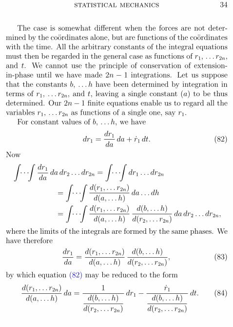
The case is somewhat different when the forces are not deter-mined by the coordinates alone, but are functions of the coordinateswith the time. All the arbitrary constants of the integral equationsmust then be regarded in the general case as functions of r1, . . . r2n,and t. We cannot use the principle of conservation of extension-in-phase until we have made 2n − 1 integrations. Let us supposethat the constants b, . . .h have been determined by integration interms of r1, . . . r2n, and t, leaving a single constant (a) to be thusdetermined. Our 2n− 1 finite equations enable us to regard all thevariables r1, . . . r2n as functions of a single one, say r1.
For constant values of b, . . .h, we have
dr1 =dr1
dada+ r1 dt. (82)
Now∫· · ·∫dr1
dada dr2 . . . dr2n =
∫· · ·∫dr1 . . . dr2n
=
∫· · ·∫d(r1, . . . r2n)
d(a, . . . h)da . . . dh
=
∫· · ·∫d(r1, . . . r2n)
d(a, . . . h)
d(b, . . . h)
d(r2, . . . r2n)da dr2 . . . dr2n,
where the limits of the integrals are formed by the same phases. Wehave therefore
dr1
da=d(r1, . . . r2n)
d(a, . . . h)
d(b, . . . h)
d(r2, . . . r2n), (83)
by which equation (82) may be reduced to the form
d(r1, . . . r2n)
d(a, . . . h)da =
1
d(b, . . . h)
d(r2, . . . r2n)
dr1 −r1
d(b, . . . h)
d(r2, . . . r2n)
dt. (84)

statistical mechanics 35
Now we know by (71) that the coefficient of da is a functionof a, . . .h. Therefore, as b, . . .h are regarded as constant in theequation, the first number represents the differential of a functionof a, . . .h, which we may denote by a′. We have then
da′ =1
d(b, . . . h)
d(r2, . . . r2n)
dr1 −r1
d(b, . . . h)
d(r2, . . . r2n)
dt, (85)
which may be integrated by quadratures. In this case we may saythat the principle of conservation of extension-in-phase has suppliedthe ‘multiplier’
1
d(b, . . . h)
d(r2, . . . r2n)
dr1 (86)
for the integration of the equation
dr1 − r1 dt = 0. (87)
The system of arbitrary constants a′, b, . . .h has evidently thesame properties which were noticed in regard to the system a,b′, . . .h.

IV.
ON THE DISTRIBUTION IN PHASE CALLED CANONICAL,IN WHICH THE INDEX OF PROBABILITY IS A LINEAR
FUNCTION OF THE ENERGY.
Let us now give our attention to the statistical equilibrium of en-sembles of conservation systems, especially to those cases and prop-erties which promise to throw light on the phenomena of thermo-dynamics.
The condition of statistical equilibrium may be expressed in theform∗ ∑(
dP
dp1
p1 +dP
dq1
q1
)= 0, (88)
where P is the coefficient of probability, or the quotient of thedensity-in-phase by the whole number of systems. To satisfy thiscondition, it is necessary and sufficient that P should be a functionof the p’s and q’s (the momenta and coordinates) which does notvary with the time in a moving system. In all cases which we arenow considering, the energy, or any function of the energy, is sucha function.
P = func.(ε)
will therefore satisfy the equation, as indeed appears identically ifwe write it in the form∑(
dP
dp1
dε
dp1
− dP
dq1
dε
dq1
)= 0.
∗See equations (20), (41), (42), also the paragraph following equation (20).The positions of any external bodies which can affect the systems are heresupposed uniform for all the systems and constant in time.

statistical mechanics 37
There are, however, other conditions to which P is subject,which are not so much conditions of statistical equilibrium, as con-ditions implicitly involved in the definition of the coefficient of prob-ability, whether the case is one of equilibrium or not. These are:that P should be single-valued, and neither negative nor imaginaryfor any phase, and that expressed by equation (46), viz.,∫
all· · ·phases
∫P dp1 . . . dqn = 1. (89)
These considerations exclude
P = ε× constant,
as well asP = constant,
as cases to be considered.The distribution represented by
η = logP =ψ − ε
Θ, (90)
or
P = eψ−εΘ , (91)
where Θ and ψ are constants, and Θ positive, seems to represent themost simple case conceivable, since it has the property that whenthe system consists of parts with separate energies, the laws of thedistribution in phase of the separate parts are of the same nature,—a property which enormously simplifies the discussion, and is thefoundation of extremely important relations to thermodynamics.The case is not rendered less simple by the divisor Θ, (a quantityof the same dimensions as ε,) but the reverse, since it makes the

statistical mechanics 38
distribution independent of the units employed. The negative signof ε is required by (89), which determines also the value of ψ forany given Θ, viz.,
e−ψΘ =
∫all· · ·
phases
∫e−
εΘ dp1 . . . dqn. (92)
When an ensemble of systems is distributed in phase in the man-ner described, i.e., when the index of probability is a linear func-tion of the energy, we shall say that the ensemble is canonicallydistributed, and shall call the divisor of the energy (Θ) the modulusof distribution.
The fractional part of an ensemble canonically distributed whichlies within any given limits of phase is therefore represented by themultiple integral ∫
· · ·∫eψ−εΘ dp1 . . . dqn (93)
taken within those limits. We may express the same thing by sayingthat the multiple integral expresses the probability that an unspec-ified system of the ensemble (i.e., one of which we only know thatit belongs to the ensemble) falls within the given limits.
Since the value of a multiple integral of the form (23) (which wehave called an extension-in-phase) bounded by any given phases isindependent of the system of coordinates by which it is evaluated,the same must be true of the multiple integral in (92), as appearsat once if we divide up this integral into parts so small that theexponential factor may be regarded as constant in each. The valueof ψ is therefore independent of the system of coordinates employed.
It is evident that ψ might be defined as the energy for which thecoefficient of probability of phase has the value unity. Since howeverthis coefficient has the dimensions of the inverse nth power of the

statistical mechanics 39
product of energy and time,∗ the energy represented by ψ is notindependent of the units of energy and time. But when these unitshave been chosen, the definition of ψ will involve the same arbitraryconstant as ε, so that, while in any given case the numerical valuesof ψ or ε will be entirely indefinite until the zero of energy hasalso been fixed for the system considered, the difference ψ − ε willrepresent a perfectly definite amount of energy, which is entirelyindependent of the zero of energy which we may choose to adopt.
It is evident that the canonical distribution is entirely deter-mined by the modulus (considered as a quantity of energy) and thenature of the system considered, since when equation (92) is sat-isfied the value of the multiple integral (93) is independent of theunits and of the coordinates employed, and of the zero chosen forthe energy of the system.
In treating of the canonical distribution, we shall always sup-pose the multiple integral in equation (92) to have a finite value, asotherwise the coefficient of probability vanishes, and the law of dis-tribution becomes illusory. This will exclude certain cases, but notsuch apparently, as will affect the value of our results with respectto their bearing on thermodynamics. It will exclude, for instance,cases in which the system or parts of it can be distributed in un-limited space (or in a space which has limits, but is still infinite involume), while the energy remains beneath a finite limit. It also ex-cludes many cases in which the energy can decrease without limit,as when the system contains material points which attract one an-other inversely as the squares of their distances. Cases of materialpoints attracting each other inversely as the distances would be ex-cluded for some values of Θ, and not for others. The investigation ofsuch points is best left to the particular cases. For the purposes of a
∗See Chapter I, p. 20.

statistical mechanics 40
general discussion, it is sufficient to call attention to the assumptionimplicitly involved in the formula (92).∗
The modulus Θ has properties analogous to those of temperaturein thermodynamics. Let the system A be defined as one of anensemble of systems of m degrees of freedom distributed in phasewith a probability-coefficient
eψA−εA
Θ ,
and the system B as one of an ensemble of systems of n degrees offreedom distributed in phase with a probability-coefficient
eψB−εB
Θ ,
which has the same modulus. Let q1, . . . qm, p1, . . . pm be thecoordinates and momenta of A, and qm+1, . . . qm+n, pm+1, . . . pm+n
those of B. Now we may regard the systems A and B as togetherforming a system C, having m + n degrees of freedom, and thecoordinates and momenta q1, . . . qm+n, p1, . . . pm+n. The probabil-ity that the phase of the system C, as thus defined, will fall withinthe limits
dp1, . . . dpm+n, dq1, . . . dqm+n
is evidently the product of the probabilities that the systems A andB will each fall within the specified limits, viz.,
eψA+ψB−εA−εB
Θ dp1 . . . dpm+n dq1 . . . dqm+n. (94)
∗It will be observed that similar limitations exist in thermodynamics. Inorder that a mass of gas can be in thermodynamic equilibrium, it is necessarythat it be enclosed. There is no thermodynamic equilibrium of a (finite) mass ofgas in an infinite space. Again, that two attracting particles should be able to doan infinite amount of work in passing from one configuration (which is regardedas possible) to another, is a notion which, although perfectly intelligible in amathematical formula, is quite foreign to our ordinary conceptions of matter.

statistical mechanics 41
We may therefore regard C as an undetermined system of an en-semble distributed with the probability-coefficient
eψA+ψB−(εA+εB)
Θ , (95)
an ensemble which might be defined as formed by combining eachsystem of the first ensemble with each of the second. But sinceεA + εB is the energy of the whole system, and ψA and ψB areconstants, the probability-coefficient is of the general form which weare considering, and the ensemble to which it relates is in statisticalequilibrium and is canonically distributed.
This result, however, so far as statistical equilibrium is con-cerned, is rather nugatory, since conceiving of separate systems asforming a single system does not create any interaction betweenthem, and if the systems combined belong to ensembles in statisticalequilibrium, to say that the ensemble formed by such combinationsas we have supposed is in statistical equilibrium, is only to repeatthe data in different words. Let us therefore suppose that in form-ing the system C we add certain forces acting between A and B,and having the force-function −εAB. The energy of the system Cis now εA + εB + εAB, and an ensemble of such systems distributedwith a density proportional to
e−(εA+εB+εAB)
Θ (96)
would be in statistical equilibrium. Comparing this with theprobability-coefficient of C given above (95), we see that if wesuppose εAB (or rather the variable part of this term when weconsider all possible configurations of the systems A and B) to beinfinitely small, the actual distribution in phase of C will differ
statistical mechanics 42
infinitely little from one of statistical equilibrium, which is equiva-lent to saying that its distribution in phase will vary infinitely littleeven in a time indefinitely prolonged.∗ The case would be entirelydifferent if A and B belonged to ensembles having different moduli,say ΘA and ΘB. The probability-coefficient of C would then be
eψA−εA
ΘA+ψB−εB
ΘB , (97)
which is not approximately proportional to any expression of theform (96).
Before proceeding farther in the investigation of the distributionin phase which we have called canonical, it will be interesting to seewhether the properties with respect to statistical equilibrium whichhave been described are peculiar to it, or whether other distributionsmay have analogous properties.
Let η′ and η′′ be the indices of probability in two independentensembles which are each in statistical equilibrium, then η′+η′′ willbe the index in the ensemble obtained by combining each systemof the first ensemble with each system of the second. This third
∗It will be observed that the above condition relating to the forces which actbetween the different systems is entirely analogous to that which must hold inthe corresponding case in thermodynamics. The most simple test of the equalityof temperature of two bodies is that they remain in equilibrium when broughtinto thermal contact. Direct thermal contact implies molecular forces actingbetween the bodies. Now the test will fail unless the energy of these forces canbe neglected in comparison with the other energies of the bodies. Thus, in thecase of energetic chemical action between the bodies, or when the number ofparticles affected by the forces acting between the bodies is not negligible incomparison with the whole number of particles (as when the bodies have theform of exceedingly thin sheets), the contact of bodies of the same temperaturemay produce considerable thermal disturbance, and thus fail to afford a reliablecriterion of the equality of temperature.

statistical mechanics 43
ensemble will of course be in statistical equilibrium, and the functionof phase η′+η′′ will be a constant of motion. Now when infinitesimalforces are added to the compound systems, if η′ + η′′ or a functiondiffering infinitesimally from this is still a constant of motion, itmust be on account of the nature of the forces added, or if theiraction is not entirely specified, on account of conditions to whichthey are subject. Thus, in the case already considered, η′ + η′′ is afunction of the energy of the compound system, and the infinitesimalforces added are subject to the law of conservation of energy.
Another natural supposition in regard to the added forces is thatthey should be such as not to affect the moments of momentum ofthe compound system. To get a case in which moments of mo-mentum of the compound system shall be constants of motion, wemay imagine material particles contained in two concentric spheri-cal shells, being prevented from passing the surfaces bounding theshells by repulsions acting always in lines passing through the com-mon centre of the shells. Then, if there are no forces acting betweenparticles in different shells, the mass of particles in each shell willhave, besides its energy, the moments of momentum about threeaxes through the centre as constants of motion.
Now let us imagine an ensemble formed by distributing in phasethe system of particles in one shell according to the index of prob-ability
A− ε
Θ+ω1
Ω1
+ω2
Ω2
+ω3
Ω3
, (98)
where ε denotes the energy of the system, and ω1, ω2, ω3, its threemoments of momentum, and the other letters constants. In likemanner let us imagine a second ensemble formed by distributingin phase the system of particles in the other shell according to the

statistical mechanics 44
index
A′ − ε′
Θ+ω′1Ω1
+ω′2Ω2
+ω′3Ω3
, (99)
where the letters have similar significations, and Θ, Ω1, Ω2, Ω3 thesame values as in the preceding formula. Each of the two ensembleswill evidently be in statistical equilibrium, and therefore also theensemble of compound systems obtained by combining each systemof the first ensemble with each of the second. In this third ensemblethe index of probability will be
A+ A′ − ε+ ε′
Θ+ω1 + ω′1
Ω1
+ω2 + ω′2
Ω2
+ω3 + ω′3
Ω3
, (100)
where the four numerators represent functions of phase which areconstants of motion for the compound systems.
Now if we add in each system of this third ensemble infinitesimalconservative forces of attraction or repulsion between particles indifferent shells, determined by the same law for all the systems, thefunctions ω1 + ω′1, ω2 + ω′2, and ω3 + ω′3 will remain constants ofmotion, and a function differing infinitely little from ε1 +ε′ will be aconstant of motion. It would therefore require only an infinitesimalchange in the distribution in phase of the ensemble of compoundsystems to make it a case of statistical equilibrium. These propertiesare entirely analogous to those of canonical ensembles.∗
∗It would not be possible to omit the term relating to energy in the aboveindices, since without this term the condition expressed by equation (89) cannotbe satisfied.
The consideration of the above case of statistical equilibrium may be made thefoundation of the theory of the thermodynamic equilibrium of rotating bodies,—a subject which has been treated by Maxwell in his memoir “On Boltzmann’stheorem on the average distribution of energy in a system of material points.”Cambr. Phil. Trans., vol. XII, p. 547, (1878).
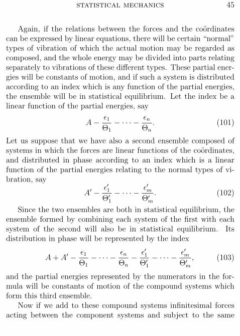
statistical mechanics 45
Again, if the relations between the forces and the coordinatescan be expressed by linear equations, there will be certain “normal”types of vibration of which the actual motion may be regarded ascomposed, and the whole energy may be divided into parts relatingseparately to vibrations of these different types. These partial ener-gies will be constants of motion, and if such a system is distributedaccording to an index which is any function of the partial energies,the ensemble will be in statistical equilibrium. Let the index be alinear function of the partial energies, say
A− ε1Θ1
− · · · − εnΘn
. (101)
Let us suppose that we have also a second ensemble composed ofsystems in which the forces are linear functions of the coordinates,and distributed in phase according to an index which is a linearfunction of the partial energies relating to the normal types of vi-bration, say
A′ − ε′1Θ′1− · · · − ε′m
Θ′m. (102)
Since the two ensembles are both in statistical equilibrium, theensemble formed by combining each system of the first with eachsystem of the second will also be in statistical equilibrium. Itsdistribution in phase will be represented by the index
A+ A′ − ε1Θ1
− · · · − εnΘn
− ε′1Θ′1− · · · − ε′m
Θ′m, (103)
and the partial energies represented by the numerators in the for-mula will be constants of motion of the compound systems whichform this third ensemble.
Now if we add to these compound systems infinitesimal forcesacting between the component systems and subject to the same

statistical mechanics 46
general law as those already existing, viz., that they are conserva-tive and linear functions of the coordinates, there will still be n+mtypes of normal vibration, and n + m partial energies which areindependent constants of motion. If all the original n + m normaltypes of vibration have different periods, the new types of normalvibration will differ infinitesimally from the old, and the new par-tial energies, which are constants of motion, will be nearly the samefunctions of phase as the old. Therefore the distribution in phaseof the ensemble of compound systems after the addition of the sup-posed infinitesimal forces will differ infinitesimally from one whichwould be in statistical equilibrium.
The case is not so simple when some of the normal types of mo-tion have the same periods. In this case the addition of infinitesimalforces may completely change the normal types of motion. But thesum of the partial energies for all the original types of vibrationwhich have any same period, will be nearly identical (as a functionof phase, i.e., of the coordinates and momenta,) with the sum ofthe partial energies for the normal types of vibration which havethe same, or nearly the same, period after the addition of the newforces. If, therefore, the partial energies in the indices of the firsttwo ensembles (101) and (102) which relate to types of vibrationhaving the same periods, have the same divisors, the same willbe true of the index (103) of the ensemble of compound systems,and the distribution represented will differ infinitesimally from onewhich would be in statistical equilibrium after the addition of thenew forces.∗
∗It is interesting to compare the above relations with the laws respectingthe exchange of energy between bodies by radiation, although the phenomenaof radiations lie entirely without the scope of the present treatise, in which thediscussion is limited to systems of a finite number of degrees of freedom.

statistical mechanics 47
The same would be true if in the indices of each of the originalensembles we should substitute for the term or terms relating toany period which does not occur in the other ensemble, any func-tion of the total energy related to that period, subject only to thegeneral limitation expressed by equation(89). But in order that theensemble of compound systems (with the added forces) shall alwaysbe approximately in statistical equilibrium, it is necessary that theindices of the original ensembles should be linear functions of thosepartial energies which relate to vibrations of periods common tothe two ensembles, and that the coefficients of such partial energiesshould be the same in the two indices.∗
The properties of canonically distributed ensembles of systemswith respect to the equilibrium of the new ensembles which maybe formed by combining each system of one ensemble with eachsystem of another, are therefore not peculiar to them in the sensethat analogous properties do not belong to some other distributionsunder special limitations in regard to the systems and forces consid-ered. Yet the canonical distribution evidently constitutes the mostsimple case of the kind, and that for which the relations describedhold with the least restrictions.
Returning to the case of the canonical distribution, we shall findother analogies with thermodynamic systems, if we suppose, as inthe preceding chapters,† that the potential energy (εq) depends notonly upon the coordinates q1, . . . qn which determine the configura-tion of the system, but also upon certain coordinates a1, a2, etc. of
∗The above may perhaps be sufficiently illustrated by the simple case wheren = 1 in each system. If the periods are different in the two systems, they maybe distributed according to any functions of the energies: but if the periods arethe same they must be distributed canonically with same modulus in order thatthe compound ensemble with additional forces may be in statistical equilibrium.
†See especially Chapter I, p. 2.

statistical mechanics 48
bodies which we call external, meaning by this simply that they arenot to be regarded as forming any part of the system, although theirpositions affect the forces which act on the system. The forces ex-erted by the system upon these external bodies will be representedby −dεq/da1, −dεq/da2, etc., while −dεq/dq1, . . .−dεq/dqn representall the forces acting upon the bodies of the system, including thosewhich depend upon the position of the external bodies, as well asthose which depend only upon the configuration of the system itself.It will be understood that εp depends only upon q1, . . . qn p1, . . . pn,in other words, that the kinetic energy of the bodies which we callexternal forms no part of the kinetic energy of the system. It followsthat we may write
dε
da1
=dεqda1
= −A1, (104)
although a similar equation would not hold for differentiations rel-ative to the internal coordinates.
We always suppose these external coordinates to have the samevalues for all systems of any ensemble. In the case of a canonicaldistribution, i.e., when the index of probability of phase is a linearfunction of the energy, it is evident that the values of the externalcoordinates will affect the distribution, since they affect the energy.In the equation
e−ψΘ =
∫all· · ·
phases
∫e−
εΘ dp1 . . . dqn, (105)
by which ψ may be determined, the external coordinates, a1, a2,etc., contained implicitly in ε, as well as Θ, are to be regarded asconstant in the integrations indicated. The equation indicates thatψ is a function of these constants. If we imagine their values varied,and the ensemble distributed canonically according to their new

statistical mechanics 49
values, we have by differentiation of the equation,
e−ψΘ
(− 1
Θdψ +
ψ
Θ2dΘ
)=
1
Θ2dΘ
∫all· · ·
phases
∫εe−
εΘ dp1 . . . dqn
− 1
Θda1
∫all· · ·
phases
∫dε
da1
e−εΘ dp1 . . . dqn
− 1
Θda2
∫all· · ·
phases
∫dε
da2
e−εΘ dp1 . . . dqn − etc., (106)
or, multiplying by Θ eψΘ , and setting
− dε
da1
= A1, − dε
da2
= A2, etc.,
− dψ +ψ
ΘdΘ =
1
ΘdΘ
∫all· · ·
phases
∫εe
ψ−εΘ dp1 . . . dqn
+ da1
∫all· · ·
phases
∫A1 e
ψ−εΘ dp1 . . . dqn
+ da2
∫all· · ·
phases
∫A2 e
ψ−εΘ dp1 . . . dqn + etc. (107)
Now the average value in the ensemble of any quantity (which weshall denote in general by a horizontal line above the proper symbol)is determined by the equation
u =
∫all· · ·
phases
∫u e
ψ−εΘ dp1 . . . dqn. (108)
Comparing this with the preceding equation, we have
dψ =ψ
ΘdΘ− ε
ΘdΘ− A1 da1 − A2 da2 − etc. (109)

statistical mechanics 50
Or, sinceψ − ε
Θ= η, (110)
and
ψ − εΘ
= η, (111)
dψ = η dΘ− A1 da1 − A2 da2 − etc. (112)
Moreover, since (111) gives
dψ − dε = Θ dη + η dΘ, (113)
we have also
dε = −Θ dη − A1 da1 − A2 da2 − etc. (114)
This equation, if we neglect the sign of averages, is identical inform with the thermodynamic equation
dη =dε+ A1 da1 + A2 da2 + etc.
T, (115)
ordε = T dη − A1 da1 − A2 da2 − etc. (116)
which expresses the relation between the energy, temperature, andentropy of a body in thermodynamic equilibrium, and the forceswhich it exerts on external bodies,—a relation which is the math-ematical expression of the second law of thermodynamics for re-versible changes. The modulus in the statistical equation corre-sponds to temperature in the thermodynamic equation, and theaverage index of probability with its sign reversed corresponds toentropy. But in the thermodynamic equation the entropy (η) is a

statistical mechanics 51
quantity which is only defined by the equation itself, and incom-pletely defined in that the equation only determines its differential,and the constant of integration is arbitrary. On the other hand,the η in the statistical equation has been completely defined as theaverage value in a canonical ensemble of systems of the logarithmof the coefficient of probability of phase.
We may also compare equation (112) with the thermodynamicequation
dψ = −η dT − A1 da1 − A2 da2 − etc., (117)
where ψ represents the function obtained by subtracting the productof the temperature and entropy from the energy.
How far, or in what sense, the similarity of these equations con-stitutes any demonstration of the thermodynamic equations, or ac-counts for the behavior of material systems, as described in the the-orems of thermodynamics, is a question of which we shall postponethe consideration until we have further investigated the propertiesof an ensemble of systems distributed in phase according to the lawwhich we are considering. The analogies which have been pointedout will at least supply the motive for this investigation, which willnaturally commence with the determination of the average valuesin the ensemble of the most important quantities relating to thesystems, and to the distribution of the ensemble with respect to thedifferent values of these quantities.

V.
AVERAGE VALUES IN A CANONICAL ENSEMBLE OFSYSTEMS.
In the simple but important case of a system of material points,if we use rectangular coordinates, we have for the product of thedifferentials of the coordinates
dx1 dy1 dz1 . . . dxν dyν dzν ,
and for the product of the differentials of the momenta
m1 dx1m1 dy1m1 dz1 . . .mν dxνmν dyνmν dzν .
The product of these expressions, which represents an element ofextension-in-phase, may be briefly written
m1 dx1 . . .mν dzν dx1 . . . dzν ;
and the integral∫· · ·∫eψ−εΘ m1 dx1 . . .mν dzν dx1 . . . dzν (118)
will represent the probability that a system taken at random froman ensemble canonically distributed will fall within any given limitsof phase.
In this case
ε = εq + 12m1x
21 + · · ·+ 1
2mν x
2ν , (119)
and
eψ−εΘ = e
ψ−εqΘ e−
m1x21
2Θ . . . e−mν x2
ν
2Θ . (120)

statistical mechanics 53
The potential energy (εq) is independent of the velocities, and ifthe limits of integration for the coordinates are independent of thevelocities, and the limits of the several velocities are independent ofeach other as well as of the coordinates, the multiple integral maybe resolved into the product of integrals∫
· · ·∫eψ−εq
Θ dx1 . . . dzν
∫e−
m1x21
2Θ m1dx1 . . .
∫e−
mν z2ν
2Θ mν dzν .
(121)This shows that the probability that the configuration lies withinany given limits is independent of the velocities, and that the prob-ability that any component velocity lies within any given limits isindependent of the other component velocities and of the configu-ration.
Since ∫ ∞−∞
e−m1x2
1
2Θ m1dx1 =√
2πm1Θ, (122)
and ∫ ∞−∞
12m1x
21 e−m1x2
1
2Θ m1dx1 =√
12πm1Θ3, (123)
the average value of the part of the kinetic energy due to the veloc-ity x1, which is expressed by the quotient of these integrals, is 1
2Θ.
This is true whether the average is taken for the whole ensemble orfor any particular configuration, whether it is taken without refer-ence to the other component velocities, or only those systems areconsidered in which the other component velocities have particularvalues or lie within specified limits.
The number of coordinates is 3ν or n. We have, therefore, forthe average value of the kinetic energy of a system
εp = 32νΘ = 1
2nΘ. (124)

statistical mechanics 54
This is equally true whether we take the average for the whole en-semble, or limit the average to a single configuration.
The distribution of the systems with respect to their componentvelocities follows the ‘law of errors’; the probability that the valueof any component velocity lies within any given limits being repre-sented by the value of the corresponding integral in (121) for those
limits, divided by (2πmΘ)12 , which is the value of the same integral
for infinite limits. Thus the probability that the value of x1 liesbetween any given limits is expressed by( m1
2πΘ
) 12
∫e−
m1x21
2Θ dx1. (125)
The expression becomes more simple when the velocity is expressedwith reference to the energy involved. If we set
s =(m1
2Θ
) 12x1,
the probability that s lies between any given limits is expressed by
1√π
∫e−s
2
ds. (126)
Here s is the ratio of the component velocity to that which wouldgive the energy Θ; in other words, s2 is the quotient of the energydue to the component velocity divided by Θ. The distribution withrespect to the partial energies due to the component velocities istherefore the same for all the component velocities.
The probability that the configuration lies within any given lim-its is expressed by the value of
M32 (2πΘ)
3ν2
∫· · ·∫eψ−εΘ dx1 . . . dxν (127)

statistical mechanics 55
for those limits, where M denotes the product of all the masses.This is derived from (121) by substitution of the values of the inte-grals relating to velocities taken for infinite limits.
Very similar results may be obtained in the general case of aconservative system of n degrees of freedom. Since εp is a homoge-neous quadratic function of the p’s, it may be divided into parts bythe formula
εp = 12p1dεpdp1
+ · · ·+ 12pn
dεpdpn
, (128)
where εmight be written for εp in the differential coefficients withoutaffecting the signification. The average value of the first of theseparts, for any given configuration, is expressed by the quotient∫ ∞
−∞· · ·∫ ∞−∞
12p1
dε
dp1
eψ−εΘ dp1 . . . dpn∫ ∞
−∞· · ·∫ ∞−∞
eψ−εΘ dp1 . . . dpn
. (129)
Now we have by integration by parts∫ ∞−∞
p1eψ−εΘ
dε
dp1
dp1 = Θ
∫ ∞−∞
eψ−εΘ dp1. (130)
By substitution of this value, the above quotient reduces to 12Θ,
which is therefore the average value of 12p1
dε
dp1
for the given con-
figuration. Since this value is independent of the configuration, itmust also be the average for the whole ensemble, as might easily beproved directly. (To make the preceding proof apply directly to thewhole ensemble, we have only to write dp1 . . . dqn for dp1 . . . dpn inthe multiple integrals.) This gives 1
2nΘ for the average value of the

statistical mechanics 56
whole kinetic energy for any given configuration, or for the wholeensemble, as has already been proved in the case of material points.
The mechanical significance of the several parts into which thekinetic energy is divided in equation (128) will be apparent if weimagine that by the application of suitable forces (different fromthose derived from εq and so much greater that the latter may beneglected in comparison) the system was brought from rest to thestate of motion considered, so rapidly that the configuration was notsensibly altered during the process, and in such a manner also thatthe ratios of the component velocities were constant in the process.If we write
F1 dq1 + · · ·+ Fn dqn
for the moment of these forces, we have for the period of their actionby equation (3)
p1 = −dεpdq1
− dεqdq1
+ F1 = − dε
dq1
+ F1.
The work done by the force F1 may be evaluated as follows:∫F1 dq1 =
∫p1 dq1 +
∫dε
dq1
dq1,
where the last term may be cancelled because the configuration doesnot vary sensibly during the application of the forces. (It will beobserved that the other terms contain factors which increase as thetime of the action of the forces is diminished.) We have therefore,∫
F1 dq1 =
∫p1q1 dt =
∫q1 dp1 =
q1
p1
∫p1 dp1. (131)
For since the p’s are linear functions of the q’s (with coefficientsinvolving the q’s) the supposed constancy of the q’s and of the ratios

statistical mechanics 57
of the q’s will make the ratio q1/p1 constant. The last integral isevidently to be taken between the limits zero and the value of p1
in the phase originally considered, and the quantities before theintegral sign may be taken as relating to that phase. We havetherefore ∫
F1 dq1 = 12p1q1 = 1
2p1
dε
dp1
. (132)
That is: the several parts into which the kinetic energy is dividedin equation (128) represent the amounts of energy communicatedto the system by the several forces F1, . . .Fn under the conditionsmentioned.
The following transformation will not only give the value of theaverage kinetic energy, but will also serve to separate the distribu-tion of the ensemble in configuration from its distribution in velocity.
Since 2εp is a homogeneous quadratic function of the p’s, whichis incapable of a negative value, it can always be expressed (andin more than one way) as a sum of squares of linear functions ofthe p’s.∗ The coefficients in these linear functions, like those in thequadratic function, must be regarded in the general case as functionsof the q’s. Let
2εp = u21 + u2
2 + · · ·+ u2n (133)
where u1, . . .un are such linear functions of the p’s. If we write
d(p1 . . . pn)
d(u1 . . . un)
for the Jacobian or determinant of the differential coefficients of the
∗The reduction requires only the repeated application of the process of‘completing the square’ used in the solution of quadratic equations.

statistical mechanics 58
form dp/du, we may substitute
d(p1 . . . pn)
d(u1 . . . un)du1 . . . dun
fordp1 . . . dpn
under the multiple integral sign in any of our formulae. It will beobserved that this determinant is function of the q’s alone. The signof such a determinant depends on the relative order of the variablesin the numerator and denominator. But since the suffixes of the u’sare only used to distinguish these functions from one another, andno especial relation is supposed between a p and a u which have thesame suffix, we may evidently, without loss of generality, supposethe suffixes so applied that the determinant is positive.
Since the u’s are linear functions of the p’s, when the integrationsare to cover all values of the p’s (for constant q’s) once and onlyonce, they must cover all values of the u’s once and only once, andthe limits will be ±∞ for all the u’s. Without the supposition ofthe last paragraph the upper limits would not always be +∞, as isevident on considering the effect of changing the sign of a u. Butwith the supposition which we have made (that the determinantis always positive) we may make the upper limits +∞ and thelower −∞ for all the u’s. Analogous considerations will apply wherethe integrations do not cover all values of the p’s and therefore ofthe u’s. The integrals may always be taken from a less to a greatervalue of a u.
The general integral which expresses the fractional part of theensemble which falls within any given limits of phase is thus reduced

statistical mechanics 59
to the form∫· · ·∫eψ−εq
Θd(p1 . . . pn)
d(u1 . . . un)e−
u21+···+u2
n
2Θ du1 . . . dun dq1 . . . dqn. (134)
For the average value of the part of the kinetic energy whichis represented by 1
2u2
1, whether the average is taken for the wholeensemble, or for a given configuration, we have therefore
12u2
1 =
∫ ∞−∞
12u2
1e−u2
1
2Θ du1∫ ∞−∞
e−u2
1
2Θ du1
=(1
2πΘ3)
12
(2πΘ)12
=Θ
2, (135)
and for the average of the whole kinetic energy, 12nΘ, as before.
The fractional part of the ensemble which lies within any givenlimits of configuration, is found by integrating (134) with respect tothe u’s from −∞ to +∞. This gives
(2πΘ)n2
∫· · ·∫eψ−εq
Θd(p1 . . . pn)
d(u1 . . . un)dq1 . . . dqn (136)
which shows that the value of the Jacobian is independent of themanner in which 2εp is divided into a sum of squares. We mayverify this directly, and at the same time obtain a more convenientexpression for the Jacobian, as follows.
It will be observed that since the u’S are linear functions ofthe p’s, and the p’s linear functions of the q’s, the u’s will belinear functions of the q’s, so that a differential coefficient of theform du/dq will be independent of the q’s, and function of the q’salone. Let us write dpx/duy for the general element of the Jacobian

statistical mechanics 60
determinant. We have
dpxduy
=d
duy
dε
dqx=
d
duy
r=n∑r=1
dε
dur
durdqx
=r=n∑r=1
(d2ε
duy dur
durdqx
)=
d
dqx
dε
duy=duydqx
. (137)
Therefored(p1 . . . pn)
d(u1 . . . un)=d(u1 . . . un)
d(q1 . . . qn)(138)
and (d(p1 . . . pn)
d(u1 . . . un)
)2
=
(d(u1 . . . un)
d(q1 . . . qn)
)2
=d(p1 . . . pn)
d(q1 . . . qn). (139)
These determinants are all functions of the q’s alone.∗ The lastis evidently the Hessian or determinant formed of the second dif-ferential coefficients of the kinetic energy with respect to q1, . . . qn.We shall denote it by ∆q. The reciprocal determinant
d(q1 . . . qn)
d(p1 . . . pn),
which is the Hessian of the kinetic energy regarded as function ofthe p’s, we shall denote by ∆p.
∗It will be observed that the proof of (137) depends on the linear rela-
tion between the u’s and q’s, which makesdurdqx
constant with respect to the
differentiations here considered. Compare note on p. 11.

statistical mechanics 61
If we set
e−ψpΘ =
∫ ∞−∞· · ·∫ ∞−∞
e−εpΘ ∆
12p dp1 . . . dpn
=
∫ ∞−∞· · ·∫ ∞−∞
e−u2
1−···−u2n
2Θ du1 . . . dun = (2πΘ)n2 , (140)
andψq = ψ − ψp, (141)
the fractional part of the ensemble which lies within any given limitsof configuration (136) may be written∫
· · ·∫eψq−εq
Θ ∆12q dq1 . . . dqn, (142)
where the constant ψq may be determined by the condition that theintegral extended over all configurations has the value unity.∗
∗In the simple but important case in which ∆q is independent of the q’s,and εq a quadratic function of the q’s, if we write εα for the least value of εq (orof ε) consistent with the given values of the external coordinates, the equationdetermining ψq may be written
eεα−ψq
Θ = ∆12
q
∫ ∞−∞· · ·∫ ∞−∞
e−(εq−εα)
Θ dq1 . . . dqn.
If we denote by q′1, . . . q′n the values of q1, . . . qn which give εq its least value εα,it is evident that εq − εα is a homogeneous quadratic function of the differencesq1 − q′1, etc., and that dq1, . . . dqn may be regarded as the differentials of thesedifferences. The evaluation of this integral is therefore analytically similar tothat of the integral ∫ ∞
−∞· · ·∫ ∞−∞
e−εpΘ dp1 . . . dpn,
for which we have found the value ∆− 1
2p (2πΘ)
n2 . By the same method, or by

statistical mechanics 62
analogy, we get
eεα−ψq
Θ =
(∆q
∆q
) 12
(2πΘ)n2 ,
where ∆q is the Hessian of the potential energy as function of the q’s. It will beobserved that ∆q depends on the forces of the system and is independent of themasses, while ∆q or its reciprocal ∆p depends on the masses and is indepen-dent of the forces. While each Hessian depends on the system of coordinatesemployed, the ratio ∆q/∆q is the same for all systems.
Multiplying the last equation by (140), we have
eεα−ψ
Θ =
(∆q
∆q
) 12
(2πΘ)n.
For the average value of the potential energy, we have
εq − εα =
∫ ∞−∞· · ·∫ ∞−∞
(εq − εα)e−εq−εα
Θ dq1 . . . dqn∫ ∞−∞· · ·∫ ∞−∞
e−εq−εα
Θ dq1 . . . dqn
.
The evaluation of this expression is similar to that of∫ ∞−∞· · ·∫ ∞−∞
εpe−εpΘ dp1 . . . dpn∫ ∞
−∞· · ·∫ ∞−∞
e−εpΘ dp1 . . . dpn
,
which expresses the average value of the kinetic energy, and for which we havefound the value 1
2nΘ. We have accordingly
εq − εα = 12nΘ.
Adding the equationεp = 1
2nΘ,
we haveε− εα = nΘ.

statistical mechanics 63
When an ensemble of systems is distributed in configuration inthe manner indicated in this formula, i.e., when its distribution inconfiguration is the same as that of an ensemble canonically dis-tributed in phase, we shall say, without any reference to its veloci-ties, that it is canonically distributed in configuration.
For any given configuration, the fractional part of the systemswhich lie within any given limits of velocity is represented by thequotient of the multiple integral∫
· · ·∫e−
εpΘ dp1 . . . dpn,
or its equivalent ∫· · ·∫e−u2
1−···−u2n
2Θ ∆12q du1 . . . dun,
taken within those limits divided by the value of the same integralfor the limits ±∞. But the value, of the second multiple integralfor the limits ±∞ is evidently
∆12q (2πΘ)
n2 .
We may therefore write∫· · ·∫eψp−εp
Θ du1 . . . dun, (143)
or ∫· · ·∫eψp−εp
Θ ∆12p dp1 . . . dpn, (144)
or again ∫· · ·∫eψp−εp
Θ ∆12q dq1 . . . dqn, (145)

statistical mechanics 64
for the fractional part of the systems of any given configurationwhich lie within given limits of velocity.
When systems are distributed in velocity according to these for-mulae, i.e., when the distribution in velocity is like that in an en-semble which is canonically distributed in phase, we shall say thatthey are canonically distributed in velocity.
The fractional part of the whole ensemble which falls within anygiven limits of phase, which we have before expressed in the form∫
· · ·∫eψ−εΘ dp1 . . . dpn dq1 . . . dqn, (146)
may also be expressed in the form∫· · ·∫eψ−εΘ ∆q dq1 . . . dqn dq1 . . . dqn. (147)

VI.
EXTENSION IN CONFIGURATION AND EXTENSION INVELOCITY.
The formulae relating to canonical ensembles in the closing para-graphs of the last chapter suggest certain general notions and prin-ciples, which we shall consider in this chapter, and which are not atall limited in their application to the canonical law of distribution.∗
We have seen in Chapter IV. that the nature of the distribu-tion which we have called canonical is independent of the system ofcoordinates by which it is described, being determined entirely bythe modulus. It follows that the value represented by the multipleintegral (142), which is the fractional part of the ensemble which lieswithin certain limiting configurations, is independent of the systemof coordinates, being determined entirely by the limiting configura-tions with the modulus. Now ψ, as we have already seen, representsa value which is independent of the system of coordinates by whichit is defined. The same is evidently true of ψp by equation (140),and therefore, by (141), of ψq. Hence the exponential factor in themultiple integral (142) represents a value which is independent ofthe system of coordinates. It follows that the value of a multipleintegral of the form ∫
· · ·∫
∆12q dq1 . . . dqn (148)
∗These notions and principles are in fact such as a more logical arrange-ment of the subject would place in connection with those of Chapter I., towhich they are closely related. The strict requirements of logical order havebeen sacrificed to the natural development of the subject, and very elementarynotions have been left until they have presented themselves in the study of theleading problems.

statistical mechanics 66
is independent of the system of coordinates which is employed forits evaluation, as will appear at once, if we suppose the multipleintegral to be broken up into parts so small that the exponentialfactor may be regarded as constant in each.
In the same way the formulae (144) and (145) which expressthe probability that a system (in a canonical ensemble) of givenconfiguration will fall within certain limits of velocity, show thatmultiple integrals of the form∫
· · ·∫
∆12p dp1 . . . dpn (149)
or ∫· · ·∫
∆12q dq1 . . . dqn (150)
relating to velocities possible for a given configuration, when thelimits are formed by given velocities, have values independent ofthe system of coordinates employed.
These relations may easily be verified directly. It has alreadybeen proved that
d(P1, . . . Pn)
d(p1, . . . pn)=
d(q1, . . . qn)
d(Q1, . . . Qn)=
d(q1, . . . qn)
d(Q1, . . . Qn)
where q1, . . . qn, p1, . . . pn and Q1, . . .Qn, P1, . . .Pn are two systems
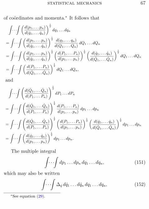
statistical mechanics 67
of coordinates and momenta.∗ It follows that∫· · ·∫ (
d(p1, . . . pn)
d(q1, . . . qn)
) 12
dq1 . . . dqn
=
∫· · ·∫ (
d(p1, . . . pn)
d(q1, . . . qn)
) 12 d(q1, . . . qn)
d(Q1, . . . Qn)dQ1 . . . dQn
=
∫· · ·∫ (
d(p1, . . . pn)
d(q1, . . . qn)
) 12(d(P1, . . . Pn)
d(p1, . . . pn)
) 12(d(q1, . . . qn)
d(Q1, . . . Qn)
) 12
dQ1 . . . dQn
=
∫· · ·∫ (
d(P1, . . . Pn)
d(Q1, . . . Qn)
) 12
dQ1 . . . dQn,
and∫· · ·∫ (
d(Q1, . . . Qn)
d(P1, . . . Pn)
) 12
dP1 . . . dPn
=
∫· · ·∫ (
d(Q1, . . . Qn)
d(P1, . . . Pn)
) 12d(P1, . . . Pn)
d(p1, . . . pn)dp1 . . . dpn
=
∫· · ·∫ (
d(Q1, . . . Qn)
d(P1, . . . Pn)
) 12 (
d(P1, . . . Pn)
d(p1, . . . pn)
) 12(d(q1, . . . qn)
d(Q1, . . . Qn)
) 12
dp1 . . . dpn
=
∫· · ·∫ (
d(q1, . . . qn)
d(p1, . . . pn)
) 12
dp1 . . . dpn.
The multiple integral∫· · ·∫dp1 . . . dpn dq1 . . . dqn, (151)
which may also be written∫· · ·∫
∆q dq1 . . . dqn dq1 . . . dqn, (152)
∗See equation (29).

statistical mechanics 68
and which, when taken within any given limits of phase, has beenshown to have a value independent of the coordinates employed, ex-presses what we have called an extension-in-phase.∗ In like mannerwe may say that the multiple integral (148) expresses an extension-in-configuration, and that the multiple integrals (149) and (150)express an extension-in-velocity. We have called
dp1 . . . dpn dq1 . . . dqn, (153)
which is equivalent to
∆q dq1 . . . dqn dq1 . . . dqn, (154)
an element of extension-in-phase. We may call
∆12q dq1 . . . dqn (155)
an element of extension-in-configuration, and
∆12p dp1 . . . dpn, (156)
or its equivalent
∆12q dq1 . . . dqn, (157)
an element of extension-in-velocity.An extension-in-phase may always be regarded as an integral
of elementary extensions-in-configuration multiplied each by anextension-in-velocity. This is evident from the formulae (151) and(152) which express an extension-in-phase, if we imagine the inte-grations relative to velocity to be first carried out.
∗See Chapter I, p. 9.

statistical mechanics 69
The product of the two expressions for an element of extension-in-velocity (149) and (150) is evidently of the same dimensions asthe product
p1 . . . pnq1 . . . qn,
that is, as the nth power of energy, since every product of theform p1q1 has the dimensions of energy. Therefore an extension-in-velocity has the dimensions of the square root of the nth powerof energy. Again we see by (155) and (156) that the product of anextension-in-configuration and an extension-in-velocity have the di-mensions of the nth power of energy multiplied by the nth power oftime. Therefore an extension-in-configuration has the dimensions ofthe nth power of time multiplied by the square root of the nth powerof energy.
To the notion of extension-in-configuration there attach them-selves certain other notions analogous to those which have presentedthemselves in connection with the notion of extension-in-phase. Thenumber of systems of any ensemble (whether distributed canoni-cally or in any other manner) which are contained in an element ofextension-in-configuration, divided by the numerical value of thatelement, may be called the density-in-configuration. That is, if acertain configuration is specified by the coordinates q1, . . . qn, andthe number of systems of which the coordinates fall between thelimits q1 and q1 + dq1, . . . qn and qn + dqn is expressed by
Dq∆12q dq1 . . . dqn, (158)
Dq will be the density-in-configuration. And if we set
eηq =Dq
N, (159)
statistical mechanics 70
where N denotes, as usual, the total number of systems in theensemble, the probability that an unspecified system of the ensemblewill fall within the given limits of configuration, is expressed by
eηq ∆12q dq1 . . . dqn. (160)
We may call eηq the coefficient of probability of the configuration,and ηq the index of probability of the configuration.
The fractional part of the whole number of systems which arewithin any given limits of configuration will be expressed by themultiple integral ∫
· · ·∫eηq ∆
12q dq1 . . . dqn. (161)
The value of this integral (taken within any given configurations)is therefore independent of the system of coordinates which is used.Since the same has been proved of the same integral without thefactor eηq , it follows that the values of ηq and Dq for a given con-figuration in a given ensemble are independent of the system ofcoordinates which is used.
The notion of extension-in-velocity relates to systems having thesame configuration.∗ If an ensemble is distributed both in configura-tion and in velocity, we may confine our attention to those systems
∗Except in some simple cases, such as a system of material points, we cannotcompare velocities in one configuration with velocities in another, and speak oftheir identity or difference except in a sense entirely artificial. We may indeedsay that we call the velocities in one configuration the same as those in anotherwhen the quantities q1, . . . qn have the same values in the two cases. But thissignifies nothing until the system of coordinates has been defined. We mightidentify the velocities in the two cases which make the quantities p1, . . . pn thesame in each. This again would signify nothing independently of the system ofcoordinates employed.

statistical mechanics 71
which are contained within certain infinitesimal limits of configu-ration, and compare the whole number of such systems with thosewhich are also contained within certain infinitesimal limits of veloc-ity. The second of these numbers divided by the first expresses theprobability that a system which is only specified as falling withinthe infinitesimal limits of configuration shall also fall within the in-finitesimal limits of velocity. If the limits with respect to velocity areexpressed by the condition that the momenta shall fall between thelimits p1 and p1 + dp1, . . . pn and pn + dpn the extension-in-velocitywithin those limits will be
∆12p dp1 . . . dpn,
and we may express the probability in question by
eηp ∆12p dp1 . . . dpn. (162)
This may be regarded as defining ηp.The probability that a system which is only specified as having a
configuration within certain infinitesimal limits shall also fall withinany given limits of velocity will be expressed by the multiple integral∫
· · ·∫eηp ∆
12p dp1 . . . dpn, (163)
or its equivalent ∫· · ·∫eηp ∆
12q dq1 . . . dqn, (164)
taken within the given limits.It follows that the probability that the system will fall within
the limits of velocity, q1 and q1 +dq1, . . . qn and qn+dqn is expressedby
eηp ∆12q dq1 . . . dqn. (165)

statistical mechanics 72
The value of the integrals (163), (164) is independent of thesystem of coordinates and momenta which is used, as is also thevalue of the same integrals without the factor eηp ; therefore thevalue of ηp must be independent of the system of coordinates andmomenta. We may call eηp the coefficient of probability of velocity,and ηp the index of probability of velocity.
Comparing (160) and (162) with (40), we get
eηqeηp = P = eη (166)
orηq + ηp = η. (167)
That is: the product of the coefficients of probability of configu-ration and of velocity is equal to the coefficient of probability ofphase; the sum of the indices of probability of configuration and ofvelocity is equal to the index of probability of phase.
It is evident that eηq and eηp have the dimensions of the recipro-cals of extension-in-configuration and extension-in-velocity respec-
tively, i.e., the dimensions of t−nε−n2 and ε−
n2 , where t represents
any time, and ε any energy. If, therefore, the unit of time is multi-plied by ct, and the unit of energy by cε, every ηq will be increasedby the addition of
n log ct + 12n log cε, (168)
and every ηp by the addition of
12n log cε.
∗ (169)
∗Compare (47) in Chapter I.

statistical mechanics 73
It should be observed that the quantities which have been calledextension-in-configuration and extension-in-velocity are not, as theterms might seem to imply, purely geometrical or kinematical con-ceptions. To express their nature more fully, they might appropri-ately have been called, respectively, the dynamical measure of theextension in configuration, and the dynamical measure of the exten-sion in velocity. They depend upon the masses, although not uponthe forces of the system. In the simple case of material points, whereeach point is limited to a given space, the extension-in-configurationis the product of the volumes within which the several points areconfined (these may be the same or different), multiplied by thesquare root of the cube of the product of the masses of the severalpoints. The extension-in-velocity for such systems is most easily de-fined as the extension-in-configuration of systems which have movedfrom the same configuration for the unit of time with the given ve-locities.
In the general case, the notions of extension-in-configuration andextension-in-velocity may be connected as follows.
If an ensemble of similar systems of n degrees of freedom have thesame configuration at a given instant, but are distributed through-out any finite extension-in-velocity, the same ensemble after an in-finitesimal interval of time δt will be distributed throughout an ex-tension in configuration equal to its original extension-in-velocitymultiplied by δtn.
In demonstrating this theorem, we shall write q′1, . . . q′n for theinitial values of the coordinates. The final values will evidently beconnected with the initial by the equations
q1 − q′1 = q1 δt, . . . , qn − q′n = qn δt. (170)
Now the original extension-in-velocity is by definition represented

statistical mechanics 74
by the integral ∫· · ·∫
∆12q dq1 . . . dqn, (171)
where the limits may be expressed by an equation of the form
F (q1, . . . qn) = 0. (172)
The same integral multiplied by the constant δtn may be written∫· · ·∫
∆12q d(q1 δt) . . . d(qn δt), (173)
and the limits may be written
F (q1, . . . qn) = f(q1 δt, . . . qn δt) = 0. (174)
(It will be observed that δt as well as ∆q is constant in the integra-tions.) Now this integral is identically equal to∫
· · ·∫
∆12q d(q1 − q′1) . . . d(qn − q′n), (175)
or its equivalent ∫· · ·∫
∆12q dq1 . . . dqn, (176)
with limits expressed by the equation
f(q1 − q′1, . . . qn − q′n) = 0. (177)
But the systems which initially had velocities satisfying the equa-tion (172) will after the interval δt have configurations satisfyingequation (177). Therefore the extension-in-configuration repre-sented by the last integral is that which belongs to the systems

statistical mechanics 75
which originally had the extension-in-velocity represented by theintegral (171).
Since the quantities which we have called extensions-in-phase,extensions-in-configuration, and extensions-in-velocity are indepen-dent of the nature of the system of coordinates used in their defi-nitions, it is natural to seek definitions which shall be independentof the use of any coordinates. It will be sufficient to give the fol-lowing definitions without formal proof of their equivalence withthose given above, since they are less convenient for use than thosefounded on systems of coordinates, and since we shall in fact haveno occasion to use them.
We commence with the definition of extension-in-velocity. Wemay imagine n independent velocities, V1, . . .Vn of which a systemin a given configuration is capable. We may conceive of the systemas having a certain velocity V0 combined with a part of each ofthese velocities V1, . . .Vn. By a part of V1 is meant a velocity ofthe same nature as V1 but in amount being anything between zeroand V1. Now all the velocities which may be thus described maybe regarded as forming or lying in a certain extension of which wedesire a measure. The case is greatly simplified if we suppose thatcertain relations exist between the velocities V1, . . .Vn viz.: thatthe kinetic energy due to any two of these velocities combined isthe sum of the kinetic energies due to the velocities separately. Inthis case the extension-in-motion is the square root of the product ofthe doubled kinetic energies due to the n velocities V1, . . .Vn takenseparately.
The more general case may be reduced to this simpler case asfollows. The velocity V2 may always be regarded as composed of twovelocities V ′2 and V ′′2 , of which V ′2 is of the same nature as V1, (it maybe more or less in amount, or opposite in sign,) while V ′′2 satisfies the

statistical mechanics 76
relation that the kinetic energy due to V1 and V ′′2 combined is thesum of the kinetic energies due to these velocities taken separately.And the velocity V3 may be regarded as compounded of three, V ′3 ,V ′′3 , V ′′′3 , of which V ′3 is of the same nature as V1, V ′′3 of the samenature as V ′′2 , while V ′′′3 satisfies the relations that if combined eitherwith V1 or V ′′2 the kinetic energy of the combined velocities is thesum of the kinetic energies of the velocities taken separately. Whenall the velocities V2, . . .Vn have been thus decomposed, the squareroot of the product of the doubled kinetic energies of the severalvelocities V1, V ′′2 . V ′′′3 , etc., will be the value of the extension-in-velocity which is sought.
This method of evaluation of the extension-in-velocity which weare considering is perhaps the most simple and natural, but the re-sult may be expressed in a more symmetrical form. Let us write ε12
for the kinetic energy of the velocities V1 and V2 combined, dimin-ished by the sum of the kinetic energies due to the same velocitiestaken separately. This may be called the mutual energy of thevelocities V1 and V2. Let the mutual energy of every pair of thevelocities V1, . . .Vn be expressed in the same way. Analogy wouldmake ε11 represent the energy of twice V1 diminished by twice theenergy of V1, i.e., ε11 would represent twice the energy of V1, al-though the term mutual energy is hardly appropriate to this case.At all events, let ε11 have this signification, and ε22 represent twicethe energy of V2, etc. The square root of the determinant∣∣∣∣∣∣∣∣
ε11 ε12 · · · ε1nε21 ε22 · · · ε2n· · · · · · · · · · · ·εn1 εn2 · · · εnn
∣∣∣∣∣∣∣∣represents the value of the extension-in-velocity determined asabove described by the velocities V1, . . .Vn.

statistical mechanics 77
The statements of the preceding paragraph may be readilyproved from the expression (157) on page 68, viz.,
∆12q dq1 . . . dqn
by which the notion of an element of extension-in-velocity wasoriginally defined. Since ∆q in this expression represents the deter-minant of which the general element is
d2ε
dqi dqj
the square of the preceding expression represents the determinantof which the general element is
d2ε
dqi dqjdqi dqj.
Now we may regard the differentials of velocity dqi, dqj as them-selves infinitesimal velocities. Then the last expression representsthe mutual energy of these velocities, and
d2ε
dq2i
dq2i
represents twice the energy due to the velocity dqi.The case which we have considered is an extension-in-velocity of
the simplest form. All extensions-in-velocity do not have this form,but all may be regarded as composed of elementary extensions ofthis form, in the same manner as all volumes may be regarded ascomposed of elementary parallelepipeds.
Having thus a measure of extension-in-velocity founded, it willbe observed, on the dynamical notion of kinetic energy, and not

statistical mechanics 78
involving an explicit mention of coordinates, we may derive from ita measure of extension-in-configuration by the principle connectingthese quantities which has been given in a preceding paragraph ofthis chapter.
The measure of extension-in-phase may be obtained from that ofextension-in-configuration and of extension-in-velocity. For to everyconfiguration in an extension-in-phase there will belong a certainextension-in-velocity, and the integral of the elements of extension-in-configuration within any extension-in-phase multiplied each byits extension-in-velocity is the measure of the extension-in-phase.

VII.
FARTHER DISCUSSION OF AVERAGES IN A CANONICALENSEMBLE OF SYSTEMS.
Returning to the case of a canonical distribution, we have for theindex of probability of configuration
ηq =ψq − εq
Θ(178)
as appears on comparison of formulae (142) and (161). It followsimmediately from (142) that the average value in the ensemble ofany quantity u which depends on the configuration alone is givenby the formula
u =
∫all· · ·
config.
∫u e
ψq−εqΘ ∆
12q dq1 . . . dqn, (179)
where the integrations cover all possible configurations. The valueof ψq is evidently determined by the equation
e−ψqΘ =
∫all· · ·
config.
∫e−
εqΘ ∆
12q dq1 . . . dqn. (180)
By differentiating the last equation we may obtain results anal-ogous to those obtained in Chapter IV. from the equation
e−ψΘ =
∫all· · ·
phases
∫e−
εΘ dp1 . . . dqn.
As the process is identical, it is sufficient to give the results:
dψq = ηq dΘ− A1 da1 − A2 da2 − etc., (181)

statistical mechanics 80
or, sinceψq = εq + Θηq, (182)
and
dψq = dεq + ηq dΘ + Θ dηq, (183)
dεq = −Θ dηq − A1 da1 − A2 da2 − etc. (184)
It appears from this equation that the differential relations subsist-ing between the average potential energy in an ensemble of systemscanonically distributed, the modulus of distribution, the average in-dex of probability of configuration, taken negatively, and the averageforces exerted on external bodies, are equivalent to those enunciatedby Clausius for the potential energy of a body, its temperature, aquantity which he called the disgregation, and the forces exerted onexternal bodies.∗
For the index of probability of velocity, in the case of canonicaldistribution, we have by comparison of (144) and (163), or of (145)and (164),
ηp =ψp − εp
Θ, (185)
which gives
ηp =ψp − εp
Θ; (186)
we have alsoεp = 1
2nΘ, (187)
and by (140),ψp = −1
2nΘ log(2πΘ). (188)
∗Pogg. Ann. Bd. CXVI, S. 73, (1862); ibid., Bd. CXXV, S. 353, (1865),See also Boltzmann, Sitzb. der Wiener Akad., Bd. LXIII, S. 728, (1871).

statistical mechanics 81
From these equations we get by differentiation
dψp = ηp dΘ, (189)
anddεp = −Θ dηp. (190)
The differential relation expressed in this equation between the av-erage kinetic energy, the modulus, and the average index of prob-ability of velocity, taken negatively, is identical with that given byClausius locis citatis for the kinetic energy of a body, the temper-ature, and a quantity which he called the transformation-value ofthe kinetic energy.∗ The relations
ε = εq + εp, η = ηq + ηp
are also identical with those given by Clausius for the correspondingquantities.
Equations (112) and (181) show that if ψ or ψq is known asfunction of Θ and a1, a2, etc., we can obtain by differentiationε or εq, and A1, A2, etc. as functions of the same variables. We havein fact
ε = ψ −Θη = ψ −Θdψ
dΘ, (191)
εq = ψq −Θηq = ψq −ΘdψqdΘ
. (192)
The corresponding equation relating to kinetic energy,
εp = ψp −Θηp = ψp −ΘdψpdΘ
, (193)
∗Verwandlungswerth des Warmeinhaltes.

statistical mechanics 82
which may be obtained in the same way, may be verified by theknown relations (186), (187), and (188) between the variables. Wehave also
A1 = − dψda1
= −dψqda1
, (194)
etc., so that the average values of the external forces may be derivedalike from ψ or from ψq.
The average values of the squares or higher powers of the energies(total, potential, or kinetic) may easily be obtained by repeateddifferentiations of ψ, ψq, ψp, or ε, εq, εp, with respect to Θ. Byequation (108) we have
ε =
∫all· · ·
phases
∫ε e
ψ−εΘ dp1 . . . dqn, (195)
and differentiating with respect to Θ,
dε
dΘ=
∫all· · ·
phases
∫ (ε2 − ψε
Θ2+ε
Θ
dψ
dΘ
)eψ−εΘ dp1 . . . dqn, (196)
whence, again by (108),
dε
dΘ=ε2 − ψε
Θ2+ε
Θ
dψ
dΘ,
or
ε2 = Θ2 dε
dΘ+ ε
(ψ −Θ
dψ
dΘ
). (197)
Combining this with (191),
ε2 = ε2 + Θ2 dε
dΘ=
(ψ −Θ
dψ
dΘ
)2
−Θ3 d2ψ
dΘ2. (198)

statistical mechanics 83
In precisely the same way, from the equation
εq =
∫all· · ·
config.
∫εq e
ψq−εqΘ ∆
12q dq1 . . . dqn, (199)
we may obtain
ε2q = ε2q + Θ2dεqdΘ
=
(ψq −Θ
dψqdΘ
)2
−Θ3 d2ψqdΘ2
. (200)
In the same way also, if we confine ourselves to a particularconfiguration, from the equation
εp =
∫all· · ·
veloc.
∫εp e
ψp−εpΘ ∆
12p dp1 . . . dpn, (201)
we obtain
ε2p = ε2p + Θ2dεpdΘ
=
(ψp −Θ
dψpdΘ
)2
−Θ3 d2ψpdΘ2
, (202)
which by (187) reduces to
ε2p = (14n2 + 1
2n)Θ2. (203)
Since this value is independent of the configuration, we see that theaverage square of the kinetic energy for every configuration is thesame, and therefore the same as for the whole ensemble. Henceε2p may be interpreted as the average either for any particular con-figuration, or for the whole ensemble. It will be observed that thevalue of this quantity is determined entirely by the modulus and thenumber of degrees of freedom of the system, and is in other respectsindependent of the nature of the system.

statistical mechanics 84
Of especial importance are the anomalies of the energies, or theirdeviations from their average values. The average value of theseanomalies is of course zero. The natural measure of such anomaliesis the square root of their average square. Now
(ε− ε)2 = ε2 − ε2, (204)
identically. Accordingly
(ε− ε)2 = Θ2 dε
dΘ= −Θ3 d
2ψ
dΘ2. (205)
In like manner,
(εq − εq)2 = Θ2dεqdΘ
= −Θ3 d2ψqdΘ2
, (206)
(εp − εp)2 = Θ2dεpdΘ
= −Θ3 d2ψpdΘ2
= 12nΘ2. (207)
Hence(ε− ε)2 = (εq − εq)2 + (εp − εp)2. (208)
Equation (206) shows that the value of dεq/dΘ can never be nega-tive, and that the value of d2ψq/dΘ2 or dηq/dΘ can never be posi-tive.∗
To get an idea of the order of magnitude of these quantities, wemay use the average kinetic energy as a term of comparison, this
∗In the case discussed in the note on page 61, in which the potential energyis a quadratic function of the q’s, and ∆q independent of the q’s, we should getfor the potential energy
(εq − εq)2 = 12nΘ2,
and for the total energy(ε− ε)2 = nΘ2.

statistical mechanics 85
quantity being independent of the arbitrary constant involved inthe definition of the potential energy. Since
εp = 12nΘ,
(εp − εp)2
ε2p=
2
n, (209)
(εq − εq)2
ε2p=
2
n
dεqdεp
, (210)
(ε− ε)2
ε2p=
2
n
dε
dεp=
2
n+
2
n
dεqdεp
. (211)
These equations show that when the number of degrees of free-dom of the systems is very great, the mean squares of the anomaliesof the energies (total, potential, and kinetic) are very small in com-parison with the mean square of the kinetic energy, unless indeedthe differential coefficient dεq/dεp is of the same order of magnitudeas n. Such values of dεq/dεp can only occur within intervals (ε′′p−ε′p)which are of the order of magnitude of n−1, unless it be in cases inwhich εq is in general of an order of magnitude higher than εp.Postponing for the moment the consideration of such cases, it will
We may also write in this case,
(εq − εq)2
(εq − εα)2=
2
n,
(ε− ε)2
(ε− εα)2=
1
n.

statistical mechanics 86
be interesting to examine more closely the case of large values ofdεq/dεp within narrow limits. Let us suppose that for ε′p and ε′′p thevalue of dεq/dεp is of the order of magnitude of unity, but betweenthese values of εp very great values of the differential coefficient oc-cur. Then in the ensemble having modulus Θ′′ and average energiesε′′p and ε′′q , values of εq sensibly greater than ε′′q will be so rare thatwe may call them practically negligible. They will be still more rarein an ensemble of less modulus. For if we differentiate the equation
ηq =ψq − εq
Θ
regarding εq as constant, but Θ and therefore ψq as variable, we get(dηqdΘ
)εq
=1
Θ
dψqdΘ− ψq − εq
Θ2, (212)
whence by (192) (dηqdΘ
)εq
=εq − εq
Θ2. (213)
That is, a diminution of the modulus will diminish the probability ofall configurations for which the potential energy exceeds its averagevalue in the ensemble. Again, in the ensemble having modulus Θ′
and average energies ε′p and ε′q, values of εq sensibly less than ε′qwill be so rare as to be practically negligible. They will be stillmore rare in an ensemble of greater modulus, since by the sameequation an increase of the modulus will diminish the probability ofconfigurations for which the potential energy is less than its averagevalue in the ensemble. Therefore, for values of Θ between Θ′ and Θ′′,and of εp between ε′p and ε′′p, the individual values of εq will bepractically limited to the interval between ε′q and ε′′q .

statistical mechanics 87
In the cases which remain to be considered, viz., when dεq/dεphas very large values not confined to narrow limits, and consequentlythe differences of the mean potential energies in ensembles of differ-ent moduli are in general very large compared with the differencesof the mean kinetic energies, it appears by (210) that the anomaliesof mean square of potential energy, if not small in comparison withthe mean kinetic energy, will yet in general be very small in compar-ison with differences of mean potential energy in ensembles havingmoderate differences of mean kinetic energy,—the exceptions beingof the same character as described for the case when dεq/dεp is notin general large.
It follows that to human experience and observation with respectto such an ensemble as we are considering, or with respect to systemswhich may be regarded as taken at random from such an ensemble,when the number of degrees of freedom is of such order of magnitudeas the number of molecules in the bodies subject to our observationand experiment, ε − ε, εp − εp, εq − εq would be in general vanish-ing quantities, since such experience would not be wide enough toembrace the more considerable divergencies from the mean values,and such observation not nice enough to distinguish the ordinarydivergencies. In other words, such ensembles would appear to hu-man observation as ensembles of systems of uniform energy, and inwhich the potential and kinetic energies (supposing that there weremeans of measuring these quantities separately) had each separatelyuniform values.∗ Exceptions might occur when for particular valuesof the modulus the differential coefficient dεq/dεp takes a very largevalue. To human observation the effect would be, that in ensemblesin which Θ and εp had certain critical values, εq would be indetermi-
∗This implies that the kinetic and potential energies of individual systemswould each separately have values sensibly constant in time.

statistical mechanics 88
nate within certain limits, viz., the values which would correspondto values of Θ and εp slightly less and slightly greater than the crit-ical values. Such indeterminateness corresponds precisely to whatwe observe in experiments on the bodies which nature presents tous.∗
To obtain general formulae for the average values of powers ofthe energies, we may proceed as follows. If h is any positive wholenumber, we have identically∫
all· · ·phases
∫εh e−
εΘ dp1 . . . dqn = Θ2 d
dΘ
∫all· · ·
phases
∫εh−1 e−
εΘ dp1 . . . dqn,
(214)i.e., by (108),
εh e−ψΘ = Θ2 d
dΘ
(εh−1 e−
ψΘ
). (215)
Hence
εh e−ψΘ =
(Θ2 d
dΘ
)he−
ψΘ , (216)
and
εh = eψΘ
(Θ2 d
dΘ
)he−
ψΘ . (217)
∗As an example, we may take a system consisting of a fluid in a cylinderunder a weighted piston, with a vacuum between the piston and the top ofthe cylinder, which is closed. The weighted piston is to be regarded as a partof the system. (This is formally necessary in order to satisfy the condition ofthe invariability of the external coordinates.) It is evident that at a certaintemperature, viz., when the pressure of saturated vapor balances the weight ofthe piston, there is an indeterminateness in the values of the potential and totalenergies as functions of the temperature.

statistical mechanics 89
For h = 1, this gives
ε = −Θ2 d
dΘ
(ψ
Θ
), (218)
which agrees with (191).From (215) we have also
εh = ε εh−1 + Θ2dεh−1
dΘ=
(ε+ Θ2 d
dΘ
)εh−1, (219)
εh =
(ε+ Θ2 d
dΘ
)h−1
ε. (220)
In like manner from the identical equation∫all· · ·
config.
∫εhq e
−εqΘ ∆
12q dq1 . . . dqn
= Θ2 d
dΘ
∫all· · ·
config.
∫εh−1q e−
εqΘ ∆
12q dq1 . . . dqn, (221)
we get
εhq = eψqΘ
(Θ2 d
dΘ
)he−
ψqΘ , (222)
and
εhq =
(εq + Θ2 d
dΘ
)h−1
εq. (223)
With respect to the kinetic energy similar equations will holdfor averages taken for any particular configuration, or for the wholeensemble. But since
εp =n
2Θ,
statistical mechanics 90
the equation
εhp =
(εp + Θ2 d
dΘ
)εh−1p (224)
reduces to
εhp =
(n
2Θ + Θ2 d
dΘ
)εh−1p =
n
2
(n
2Θ + Θ2 d
dΘ
)h−1
Θ. (225)
We have therefore
ε2p =(n
2+ 1) n
2Θ2. (226)
ε3p =(n
2+ 2)(n
2+ 1) n
2Θ3. (227)
εhp =Γ(1
2n+ h)
Γ(12n)
Θh.∗ (228)
∗In the case discussed in the note on page 61 we may easily get
(εq − εα)h =
(εq − εα + Θ2 d
dΘ
)(εq − εα)h−1,
which, with
εq − εα =n
2Θ,
gives
(εq − εα)h =
(n
2Θ + Θ2 d
dΘ
)(εq − εα)h−1 =
n
2
(n
2Θ + Θ2 d
dΘ
)h−1
Θ.
Hence(εq − εα)h = εhp .
Again
(ε− εα)h =
(ε− εα + Θ2 d
dΘ
)(ε− εα)h−1,

statistical mechanics 91
The average values of the powers of the anomalies of the energiesare perhaps most easily found as follows. We have identically, sinceε is a function of Θ, while ε is a function of the p’s and q’s,
Θ2 d
dΘ
∫all· · ·
phases
∫(ε− ε)h e−
εΘ dp1 . . . dqn
=
∫all· · ·
phases
∫ [ε(ε− ε)h − h(ε− ε)h−1Θ2 dε
dΘ
]e−
εΘ dp1 . . . dqn,
(229)
i.e., by (108),
Θ2 d
dΘ
[(ε− ε)he−
ψΘ
]=
[ε(ε− ε)h − h(ε− ε)h−1Θ2 dε
dΘ
]e−
ψΘ ,
(230)or since by (218)
Θ2 d
dΘe−
ψΘ = ε e−
ψΘ ,
Θ2 d
dΘ(ε− ε)h + (ε− ε)hε = ε(ε− ε)h − h(ε− ε)h−1Θ2 dε
dΘ,
(ε− ε)h+1 = Θ2 d
dΘ(ε− ε)h + h(ε− ε)h−1Θ2 dε
dΘ. (231)
which withε− εα = nΘ
gives
(ε− εα)h =
(nΘ + Θ2 d
dΘ
)(ε− εα)h−1 = n
(nΘ + Θ2 d
dΘ
)h−1
Θ,
hence
(ε− εα)h =Γ(n+ h)
Γ(n)Θh.

statistical mechanics 92
In precisely the same way we may obtain for the potential energy
(εq − εq)h+1 = Θ2 d
dΘ(εq − εq)h + h(εq − εq)h−1Θ2dεq
dΘ. (232)
By successive applications of (231) we obtain
(ε− ε)2 = Dε,
(ε− ε)3 = D2ε,
(ε− ε)4 = D3ε+ 3(Dε)2,
(ε− ε)5 = D4ε+ 10DεD2ε,
(ε− ε)6 = D5ε+ 15DεD3ε+ 10(D2ε)2 + 15(Dε)3 etc.,
where D represents the operator Θ2d/dΘ. Similar expressions re-lating to the potential energy may be derived from (232).
For the kinetic energy we may write similar equations in whichthe averages may be taken either for a single configuration or forthe whole ensemble. But since
dεpdΘ
=n
2,
the general formula reduces to
(εp − εp)h+1 = Θ2 d
dΘ(εp − εp)h + 1
2nhΘ2(εp − εp)h−1, (233)
or
(εp − εp)h+1
εh+1p
=2Θ
n
d
dΘ
(εp − εp)hεhp
+2h
n
(εp − εp)hεhp
+2h
n
(εp − εp)h−1
εh−1p
.
(234)

statistical mechanics 93
But since identically
(εp − εp)0
ε0p= 1,
(εp − εp)1
ε1p= 0,
the value of the corresponding expression for any index will be in-dependent of Θ and the formula reduces to(
εp − εpεp
)h+1
=2h
n
(εp − εpεp
)h+
2h
n
(εp − εpεp
)h−1
; (235)
we have therefore(εp − εpεp
)0
= 1,(εp − εpεp
)1
= 0,(εp − εpεp
)2
=2
n,
(εp − εpεp
)3
=8
n2,(
εp − εpεp
)4
=48
n3+
12
n2,
etc.∗
It will be observed that when ψ or ε is given as function of Θ,all averages of the form εh or (ε− ε)h are thereby determined. Soalso if ψq or εq is given as a function of Θ, all averages of the form
εhq or (εq − εq)h are determined. But
εq = ε− 12nΘ.
∗In the case discussed in the preceding foot-notes we get easily
(εq − εq)h = (εp − εp)h,
and (εq − εqεq − εα
)h=
(εp − εpεp
)h.

statistical mechanics 94
Therefore if any one of the quantities ψ, ψq, ε, εq is known as afunction of Θ, and n is also known, all averages of any of the formsmentioned are thereby determined as functions of the same variable.In any case all averages of the form(
εp − εpεp
)hare known in terms of n alone, and have the same value whethertaken for the whole ensemble or limited to any particular configu-ration.
If we differentiate the equation∫all· · ·
phases
∫eψ−εΘ dp1 . . . dqn = 1 (236)
with respect to a1, and multiply by Θ, we have∫· · ·∫ [
dψ
da1
− dε
da1
]eψ−εΘ dp1 . . . dqn = 0. (237)
Differentiating again, with respect to a1, with respect to a2, and
For the total energy we have in this case(ε− εε− εα
)h+1
=h
n
(ε− εε− εα
)h+h
n
(ε− εε− εα
)h−1
,
(ε− εε− εα
)2
=1
n,(
ε− εε− εα
)3
=2
n2,
(ε− εε− εα
)4
=3
n2+
6
n3,
etc.

statistical mechanics 95
with respect to Θ, we have∫· · ·∫ [
d2ψ
da21
− d2ε
da21
+1
Θ
(dψ
da1
− dε
da1
)2]eψ−εΘ dp1 . . . dqn = 0,
(238)∫· · ·∫ [
d2ψ
da1 da2
− d2ε
da1 da2
+1
Θ
(dψ
da1
− dε
da1
)(dψ
da2
− dε
da2
)]eψ−εΘ dp1 . . . dqn = 0, (239)∫
· · ·∫ [
d2ψ
da1 dΘ+
(dψ
da1
− dε
da1
)(1
Θ
dψ
dΘ− ψ − ε
Θ2
)]eψ−εΘ dp1 . . . dqn = 0. (240)
The multiple integrals in the last four equations represent the aver-age values of the expressions in the brackets, which we may thereforeset equal to zero. The first gives
dψ
da1
=dε
da1
= −A1, (241)
as already obtained. With this relation and (191) we get from theother equations
(A1 − A1)2 = Θ
(d2ε
da21
− d2ψ
da21
)= Θ
(dA1
da1
− dA1
da1
), (242)
(A1 − A1)(A2 − A2) = Θ
(d2ε
da1 da2
− d2ψ
da1 da2
)= Θ
(dA1
da2
− dA1
da2
)= Θ
(dA2
da1
− dA2
da1
), (243)

statistical mechanics 96
(A1 − A1)(ε− ε) = −Θ2 d2ψ
da1 dΘ= Θ2dA1
dΘ= −Θ2 dη
da1
.
We may add for comparison equation (205), which might be derivedfrom (236) by differentiating twice with respect to Θ:
(ε− ε)2 = −Θ2 d2ψ
dΘ2= Θ2 dε
dΘ. (244)
The two last equations give
(A1 − A1)(ε− ε) =dA
dε(ε− ε)2. (245)
If ψ or ε is known as function of Θ, a1, a2, etc., (ε− ε)2
may be obtained by differentiation as function of the same vari-ables. And if ψ, or A1, or η is known as function of Θ, a1,
etc., (A1 − A1)(ε− ε) may be obtained by differentiation. But
(A1 − A1)2 and (A1 − A1)(A2 − A2) cannot be obtained in anysimilar manner. We have seen that (ε− ε)2 is in general a van-ishing quantity for very great values of n, which we may regardas contained implicitly in Θ as a divisor. The same is true of
(A1 − A1)(ε− ε). It does not appear that we can assert the same
of (A1 − A1)2 or (A1 − A1)(A2 − A2), since d2ε/da21 may be very
great. The quantities d2ε/da21 and d2ψ/da2
1 belong to the classcalled elasticities. The former expression represents an elasticitymeasured under the condition that while a1 is varied the internalcoordinates q1, . . . qn all remain fixed. The latter is an elasticitymeasured under the condition that when a1 is varied the ensembleremains canonically distributed within the same modulus. This cor-responds to an elasticity in physics measured under the conditionof constant temperature. It is evident that the former is greaterthan the latter, and it may be enormously greater.

statistical mechanics 97
The divergences of the force A1 from its average value are duein part to the differences of energy in the systems of the ensemble,and in part to the differences in the value of the forces which existin systems of the same energy. If we write A1 |ε for the average valueof A1 in systems of the ensemble which have any same energy, itwill be determined by the equation
A1 |ε =
∫· · ·∫− dε
da1
eψ−εΘ dp1 . . . dqn∫
· · ·∫eψ−εΘ dp1 . . . dqn
, (246)
where the limits of integration in both multiple integrals are twovalues of the energy which differ infinitely little, say ε and ε + dε.
This will make the factor eψ−εΘ constant within the limits of integra-
tion, and it may be cancelled in the numerator and denominator,leaving
A1 |ε =
∫· · ·∫− dε
da1
dp1 . . . dqn∫· · ·∫dp1 . . . dqn
, (247)
where the integrals as before are to be taken between ε and ε+ dε.A1 |ε is therefore independent of Θ, being a function of the energyand the external coordinates.
Now we have identically
A1 − A1 = (A1 − A1 |ε) + (A1 |ε − A1),
where A1 − A1 |ε denotes the excess of the force (tending to in-crease a1) exerted by any system above the average of such forcesfor systems of the same energy. Accordingly,
(A1 − A1)2 = (A1 − A1 |ε)2+2(A1 − A1 |ε)(A1 |ε − A1)+(A1 |ε − A1)2.

statistical mechanics 98
But the average value of (A1 − A1 |ε)(A1 |ε − A1) for systems of theensemble which have the same energy is zero, since for such systemsthe second factor is constant. Therefore the average for the wholeensemble is zero, and
(A1 − A1)2 = (A1 − A1 |ε)2 + (A1 |ε − A1)2. (248)
In the same way it may be shown that
(A1 − A1)(ε− ε) = (A1 |ε − A1)(ε− ε). (249)
It is evident that in ensembles in which the anomalies of energy ε−εmay be regarded as insensible the same will be true of the quantitiesrepresented by A1 |ε − A1.
The properties of quantities of the form A1 |ε will be fartherconsidered in Chapter X, which will be devoted to ensembles ofconstant energy.
It may not be without interest to consider some general formulaerelating to averages in a canonical ensemble, which embrace manyof the results which have been given in this chapter.
Let u be any function of the internal and external coordinateswith the momenta and modulus. We have by definition
u =
∫all· · ·
phases
∫u e
ψ−εΘ dp1 . . . dqn. (250)
If we differentiate with respect to Θ, we have
du
dΘ=
∫all· · ·
phases
∫ (du
dΘ− u
Θ2(ψ − ε) +
u
Θ
dψ
dΘ
)eψ−εΘ dp1 . . . dqn,
ordu
dΘ=du
dΘ− u(ψ − ε)
Θ2+u
Θ
dψ
dΘ. (251)

statistical mechanics 99
Setting u = 1 in this equation, we get
dψ
dΘ=ψ − ε
Θ,
and substituting this value, we have
du
dΘ=du
dΘ+uε
Θ2− uε
Θ2,
or
Θ2 du
dΘ−Θ2 du
dΘ= uε− uε = (u− u)(ε− ε). (252)
If we differentiate equation (250) with respect to a (which mayrepresent any of the external coordinates), and write A for the
force − dεda
, we get
du
da=
∫all· · ·
phases
∫ (du
da+u
Θ
dψ
da+u
ΘA
)eψ−εΘ dp1 . . . dqn,
ordu
da=du
da+u
Θ
dψ
da+uA
Θ. (253)
Setting u = 1 in this equation, we get
dψ
da= −A.
Substituting this value, we have
du
da=du
da+uA
Θ− uA
Θ, (254)
or
Θdu
da−Θ
du
da= uA− uA = (u− u)(A− A). (255)

statistical mechanics 100
Repeated applications of the principles expressed by equations(252) and (255) are perhaps best made in the particular cases. Yetwe may write (252) in this form
(ε+D)(u− u), (256)
where D represents the operator Θ2d/dΘ.Hence
(ε+D)h(u− u) = 0, (257)
where h is any positive whole number. It will be observed, that sinceε is not function of Θ, (ε + D)h may be expanded by the binomialtheorem. Or, we may write
(ε+D)u = (ε+D)u, (258)
whence(ε+D)hu = (ε+D)hu. (259)
But the operator (ε + D)h, although in some respects more simplethan the operator without the average sign on the ε, cannot beexpanded by the binomial theorem, since ε is a function of Θ withthe external coordinates.
So from equation (254) we have(A
Θ+
d
da
)(u− u) = 0, (260)
whence (A
Θ+
d
da
)h(u− u) = 0; (261)
and (A
Θ+
d
da
)u =
(A
Θ+
d
da
)u, (262)

statistical mechanics 101
whence (A
Θ+
d
da
)hu =
(A
Θ+
d
da
)hu. (263)
The binomial theorem cannot be applied to these operators.Again, if we now distinguish, as usual, the several external
coordinates by suffixes, we may apply successively to the expres-sion u− u any or all of the operators
ε+ Θ2 d
dΘ, A1 + Θ
d
da1
, A2 + Θd
da2
, etc. (264)
as many times as we choose, and in any order, the average valueof the result will be zero. Or, if we apply the same operators to u,and finally take the average value, it will be the same as the valueobtained by writing the sign of average separately as u, and on ε,A1, A2, etc., in all the operators.
If u is independent of the momenta, formulae similar to thepreceding, but having εq in place of ε, may be derived from equa-tion (179).

VIII.
ON CERTAIN IMPORTANT FUNCTIONS OF THE ENERGIESOF A SYSTEM.
In order to consider more particularly the distribution of a canonicalensemble in energy, and for other purposes, it will be convenient touse the following definitions and notations.
Let us denote by V the extension-in-phase below a certain limitof energy which we shall call ε. That is, let
V =
∫· · ·∫dp1 . . . dqn, (265)
the integration being extended (with constant values of the externalcoordinates) over all phases for which the energy is less than thelimit ε. We shall suppose that the value of this integral is notinfinite, except for an infinite value of the limiting energy. This willnot exclude any kind of system to which the canonical distributionis applicable. For if ∫
· · ·∫e−
εΘ dp1 . . . dqn
taken without limits has a finite value,∗ the less value representedby
e−εΘ
∫· · ·∫dp1 . . . dqn
taken below a limiting value of ε, and with the ε before the integralsign representing that limiting value, will also be finite. Therefore
∗This is a necessary condition of the canonical distribution. See Chapter IV,p. 39.

statistical mechanics 103
the value of V , which differs only by a constant factor, will also befinite, for finite ε. It is a function of ε and the external coordinates,a continuous increasing function of ε, which becomes infinite with ε,and vanishes for the smallest possible value of ε, or for ε = −∞, ifthe energy may be diminished without limit.
Let us also set
φ = logdV
dε. (266)
The extension in phase between any two limits of energy, ε′ and ε′′,will be represented by the integral∫ ε′′
ε′eφ dε. (267)
And in general, we may substitute eφ dε for dp1 . . . dqn in a 2n-foldintegral, reducing it to a simple integral, whenever the limits canbe expressed by the energy alone, and the other factor under theintegral sign is a function of the energy alone, or with quantitieswhich are constant in the integration.
In particular we observe that the probability that the energyof an unspecified system of a canonical ensemble lies between thelimits ε′ and ε′′ will be represented by the integral∗∫ ε′′
ε′eψ−εΘ
+φ dε, (268)
and that the average value in the ensemble of any quantity whichonly varies with the energy is given by the equation†
u =
∫ ε=∞
V=0
u eψ−εΘ
+φ dε, (269)
∗Compare equation (93).†Compare equation (108).

statistical mechanics 104
where we may regard the constant ψ as determined by the equation∗
e−ψΘ =
∫ ε=∞
V=0
e−εΘ
+φ dε. (270)
In regard to the lower limit in these integrals, it will be observedthat V = 0 is equivalent to the condition that the value of ε is theleast possible.
In like manner, let us denote by Vq the extension-in-configurationbelow a certain limit of potential energy which we may call εq. Thatis, let
Vq =
∫· · ·∫
∆12q dq1 . . . dqn, (271)
the integration being extended (with constant values of the externalcoordinates) over all configurations for which the potential energy isless than εq. Vq will be a function of εq with the external coordinates,an increasing function of εq, which does not become infinite (in suchcases as we shall consider†) for any finite value of εq. It vanishes forthe least possible value of εq, or for εq = −∞, if εq can be dimin-ished without limit. It is not always a continuous function of εq.In fact, if there is a finite extension-in-configuration of constant po-tential energy, the corresponding value of Vq will not include thatextension-in-configuration, but if εq be increased infinitesimally, thecorresponding value of Vq will be increased by that finite extension-in-configuration.
Let us also set
φq = logdVqdεq
. (272)
∗Compare equation (92).†If Vq were infinite for finite values of εq, V would evidently be infinite for
finite values of ε.

statistical mechanics 105
The extension-in-configuration between any two limits of potentialenergy ε′q and ε′′q may be represented by the integral∫ ε′′q
ε′q
eφq dεq (273)
whenever there is no discontinuity in the value of Vq as functionof εq between or at those limits, that is, whenever there is no finiteextension-in-configuration of constant potential energy between orat the limits. And in general, with the restriction mentioned, we
may substitute eφq dεq for ∆12q dq1 . . . dqn in an n-fold integral, re-
ducing it to a simple integral, when the limits are expressed bythe potential energy, and the other factor under the integral sign isa function of the potential energy, either alone or with quantitieswhich are constant in the integration.
We may often avoid the inconvenience occasioned by formulaebecoming illusory on account of discontinuities in the values of Vq asfunction of εq by substituting for the given discontinuous functiona continuous function which is practically equivalent to the givenfunction for the purposes of the evaluations desired. It only re-quires infinitesimal changes of potential energy to destroy the finiteextensions-in-configuration of constant potential energy which arethe cause of the difficulty.
In the case of an ensemble of systems canonically distributedin configuration, when Vq is, or may be regarded as, a continuousfunction of εq (within the limits considered), the probability thatthe potential energy of an unspecified system lies between the limitsε′q and ε′′q is given by the integral∫ ε′′q
ε′q
eψq−εq
Θ+φq dεq, (274)

statistical mechanics 106
where ψ may be determined by the condition that the value of theintegral is unity, when the limits include all possible values of εq. Inthe same case, the average value in the ensemble of any function ofthe potential energy is given by the equation
u =
∫ εq=∞
Vq=0
u eψ−εq
Θ+φq dεq. (275)
When Vq is not a continuous function of εq, we may write dVq foreφq dεq in these formulae.
In like manner also, for any given configuration, let us denoteby Vp the extension-in-velocity below a certain limit of kinetic en-ergy specified by εp. That is, let
Vp =
∫· · ·∫
∆12p dp1 . . . dpn, (276)
the integration being extended, with constant values of the coord-inates, both internal and external, over all values of the momenta forwhich the kinetic energy is less than the limit εp. Vp will evidently bea continuous increasing function of εp which vanishes and becomesinfinite with εp. Let us set
φp = logdVpdεp
. (277)
The extension-in-velocity between any two limits of kinetic energyε′p and ε′′p may be represented by the integral∫ ε′′p
ε′p
eφp dεp. (278)

statistical mechanics 107
And in general, we may substitute eφp dεp for ∆12p dp1 . . . dpn or
∆12q dq1 . . . dqn in an n-fold integral in which the coordinates are con-
stant, reducing it to a simple integral, when the limits are expressedby the kinetic energy, and the other factor under the integral signis a function of the kinetic energy, either alone or with quantitieswhich are constant in the integration.
It is easy to express Vp and φp in terms of εp. Since ∆p is functionof the coordinates alone, we have by definition
Vp = ∆12p
∫· · ·∫dp1 . . . dpn (279)
the limits of the integral being given by εp. That is, if
εp = F (p1, . . . pn), (280)
the limits of the integral for εp = 1, are given by the equation
F (p1, . . . pn) = 1, (281)
and the limits of the integral for εp = a2, are given by the equation
F (p1, . . . pn) = a2. (282)
But since F represents a quadratic function, this equation may bewritten
F(p1
a, . . .
pna
)= 1. (283)
The value of Vp may also be put in the form
Vp = an ∆12p
∫· · ·∫dp1
a. . . d
pna. (284)

statistical mechanics 108
Now we may determine Vp for εp = 1 from(279) where the limitsare expressed by (281), and Vp for εp = a2 from (284) taking thelimits from (283). The two integrals thus determined are evidentlyidentical, and we have
(Vp)εp=a2 = an(Vp)εp=1, (285)
i.e., Vp varies as εn2p . We may therefore set
Vp = Cεn2p , eφp =
n
2Cε
n2−1
p (286)
where C is a constant, at least for fixed values of the internalcoordinates.
To determine this constant, let us consider the case of a canonicaldistribution, for which we have∫ ∞
0
eψp−εp
Θ+φp dεp = 1,
where
eψpΘ = (2πΘ)−
n2 .
Substituting this value, and that of eφp from (286), we get
n
2C
∫ ∞0
e−εpΘ ε
n2−1
p dεp = (2πΘ)n2 ,
n
2C
∫ ∞0
e−εpΘ
(εpΘ
)n2−1
d(εp
Θ
)= (2π)
n2 ,
n
2CΓ(n
2
)= (2π)
n2 , (287)
C =(2π)
n2
Γ(12n+ 1)
.

statistical mechanics 109
Having thus determined the value of the constant C, we maysubstitute it in the general expressions (286), and obtain the fol-lowing values, which are perfectly general:
Vp =(2πεp)
n2
Γ(12n+ 1)
, (288)
eφp =(2π)
n2 ε
n2−1
p
Γ(12n)
.∗ (289)
It will be observed that the values of Vp and φp for any given εpare independent of the configuration, and even of the nature of thesystem considered, except with respect to its number of degrees offreedom.
Returning to the canonical ensemble, we may express the prob-ability that the kinetic energy of a system of a given configuration,
∗Very similar values for Vq, eφq , V , and eφ may be found in the same way
in the case discussed in the preceding foot-notes (see pages 61, 84, 90, and 93),in which εq is a quadratic function of the q’s, and ∆q independent of the q’s.In this case we have
Vq =
(∆q
∆q
) 12 (2π)
n2 (εq − εα)
n2
Γ( 12n+ 1)
,
eφq =
(∆q
∆q
) 12 (2π)
n2 (εq − εα)
n2−1
Γ( 12n)
,
V =
(∆q
∆q
) 12 (2π)n(ε− εα)n
Γ(n+ 1),
eφ =
(∆q
∆q
) 12 (2π)n(ε− εα)n−1
Γ(n).

statistical mechanics 110
but otherwise unspecified, falls within given limits, by either mem-ber of the following equation∫
eψp−εp
Θ+φp dεp =
1
Γ(12n)
∫e−
εpΘ
(εpΘ
)n2−1
d(εp
Θ
). (290)
Since this value is independent of the coordinates it also representsthe probability that the kinetic energy of an unspecified system ofa canonical ensemble falls within the limits. The form of the lastintegral also shows that the probability that the ratio of the kineticenergy to the modulus falls within given limits is independent also ofthe value of the modulus, being determined entirely by the numberof degrees of freedom of the system and the limiting values of theratio.
The average value of any function of the kinetic energy, eitherfor the whole ensemble, or for any particular configuration, is givenby
u =1
Θn2 Γ(1
2n)
∫ ∞0
u e−εpΘ ε
n2−1
p dεp.∗ (291)
∗The corresponding equation for the average value of any function of thepotential energy, when this is a quadratic function of the q’s, and ∆q is inde-pendent of the q’s, is
u =1
Θn2 Γ( 1
2n)
∫ ∞εα
u e−εq−εα
Θ (εq − εα)n2−1 dεq.
In the same case, the average value of any function of the (total) energy is givenby the equation
u =1
ΘnΓ(n)
∫ ∞0
u e−ε−εα
Θ (ε− εα)n−1 dε.

statistical mechanics 111
Thus:
εmp =Γ(m+ 1
2n)
Γ(12n)
Θm, if m+ 12n > 0;∗ (292)
V p =Γ(n)
Γ(12n+ 1)Γ(1
2n)
(2πΘ)n2 ; (293)
eφp =Γ(n− 1)
[Γ(12n)]2
(2π)n2 Θ
n2−1, if n > 1; (294)
dφpdεp
=1
Θ, if n > 2; (295)
e−φp Vp = Θ. (296)
Hence in this case
(εq − εα)m =Γ(m+ 1
2n)
Γ( 12n)
Θm, if m+ 12n > 0.
(ε− εα)m =Γ(m+ n)
Γ(n)Θm, if m+ n > 0.
e−φq Vq = e−φ V = Θ,
dφqdεq
=1
Θ, if n > 2,
and
dφ
dε=
1
Θ, if n > 1.
If n = 1, eφ = 2π and dφ/dε = 0 for any value of ε. If n = 2, the case is thesame with respect to φq.
∗This equation has already been proved for positive integral powers of thekinetic energy. See page 90.

statistical mechanics 112
If n = 2, eφp = 2π, and dφp/dεp = 0, for any value of εp.The definitions of V , Vq, and Vp give
V =
∫∫dVp dVq, (297)
where the integrations cover all phases for which the energy is lessthan the limit ε, for which the value of V is sought. This gives
V =
∫ εq=ε
Vq=0
Vp dVq, (298)
and
eφ =dV
dε=
∫ εq=ε
Vq=0
eφp dVq, (299)
where Vp and eφp are connected with Vq by the equation
εp + εq = constant = ε. (300)
If n > 2, eφp vanishes at the upper limit, i.e., for εp = 0, and weget by another differentiation
eφdφ
dε=
∫ εq=ε
Vq=0
eφpdφpdεp
dVq. (301)
We may also write
V =
∫ εq=ε
Vq=0
Vp eφq dεq, (302)
eφ =
∫ εq=ε
Vq=0
eφp+φq dεq, (303)

statistical mechanics 113
etc., when Vq is a continuous function of εq commencing with thevalue Vq = 0, or when we choose to attribute to Vq a fictitious con-tinuity commencing with the value zero, as described on page 105.
If we substitute in these equations the values of Vp and eφp whichwe have found, we get
V =(2π)
n2
Γ(12n+ 1)
∫ εq=ε
Vq=0
(ε− εq)n2 dVq, (304)
eφ =(2π)
n2
Γ(12n)
∫ εq=ε
Vq=0
(ε− εq)n2−1 dVq, (305)
where eφq dεq may be substituted for dVq in the cases above de-scribed. If, therefore, n is known, and Vq as function of εq, V and eφ
may be found by quadratures.It appears from these equations that V is always a continuous
increasing function of ε, commencing with the value V = 0, evenwhen this is not the case with respect to Vq and εq. The same istrue of eφ, when n > 2, or when n = 2 if Vq increases continuouslywith εq from the value Vq = 0.
The last equation may be derived from the preceding by dif-ferentiation with respect to ε. Successive differentiations give, ifh < 1
2n+ 1,
dhV
dεh=
∫ εq=ε
Vq=0
dhVpdεhp
dVq =(2π)
n2
Γ(12n+ 1− h)
∫ εq=ε
Vq=0
(ε− εq)n2−h dVq.
(306)dhV/dεh is therefore positive if h < 1
2n + 1. It is an increasing
function of ε, if h < 12n. If ε is not capable of being diminished
without limit, dhV/dεh vanishes for the least possible value of ε, ifh < 1
2n.

statistical mechanics 114
If n is even,
dn2 V
dεn2
= (2π)n2 (Vq)εq=ε. (307)
That is, Vq is the same function of εq as1
(2π)n2
dn2 V
dεn2
of ε.
When n is large, approximate formulae will be more available. Itwill be sufficient to indicate the method proposed, without precisediscussion of the limits of its applicability or of the degree of itsapproximation. For the value of eφ corresponding to any given ε,we have
eφ =
∫ εq=ε
Vq=0
eφp+φq dεq =
∫ ε
0
eφp+φq dεp, (308)
where the variables are connected by the equation (300). The max-imum value of φp + φq is therefore characterized by the equation
dφpdεp
=dφqdεq
. (309)
The values of εp and εq determined by this maximum we shall dis-tinguish by accents, and mark the corresponding values of functionsof εp and εq in the same way. Now we have by Taylor’s theorem
φp = φ′p +
(dφpdεp
)′(εp − ε′p) +
(d2φpdε2p
)′ (εp − ε′p)2
2+ etc. (310)
φq = φ′q +
(dφqdεq
)′(εq − ε′q) +
(d2φqdε2q
)′ (εq − ε′q)2
2+ etc. (311)
If the approximation is sufficient without going beyond the quadraticterms, since by (300)
εp − εp′ = −(εq − ε′q),

statistical mechanics 115
we may write
eφ = eφ′p+φ′q
∫ ∞−∞
e
[(d2φ′pdε2p
)′
+
(d2φ′qdε2q
)′](εq−ε′q)2
2dεq, (312)
where the limits have been made ±∞ for analytical simplicity. Thisis allowable when the quantity in the square brackets has a verylarge negative value, since the part of the integral correspondingto other than very small values of εq − ε′q may be regarded as avanishing quantity.
This gives
eφ = eφ′p+φ′q
[−2π(
d2φ′pdε2p
)′+
(d2φ′qdε2q
)′] 1
2
, (313)
or
φ = φ′p + φ′q + 12
log(2π)− 12
log
[−(d2φ′pdε2p
)′−(d2φ′qdε2q
)′]. (314)
From this equation, with (289), (300) and (309), we may determinethe value of φ corresponding to any given value of ε, when φq isknown as function of εq.
Any two systems may be regarded as together forming a thirdsystem. If we have V or φ given as function of ε for any two systems,we may express by quadratures V and φ for the system formed bycombining the two. If we distinguish by the suffixes ( )1, ( )2, ( )12
the quantities relating to the three systems, we have easily from the

statistical mechanics 116
definitions of these quantities
V12 =
∫∫dV1 dV2 =
∫V2 dV1 =
∫V1 dV2 =
∫V1e
φ2 dε2, (315)
eφ12 =
∫eφ2 dV1 =
∫eφ1 dV2 =
∫eφ1+φ2 dε2, (316)
where the double integral is to be taken within the limits
V1 = 0, V2 = 0, and ε1 + ε2 = ε12,
and the variables in the single integrals are connected by the last ofthese equations, while the limits are given by the first two, whichcharacterize the least possible values of ε1 and ε2 respectively.
It will be observed that these equations are identical in formwith those by which V and φ are derived from Vp or φp and Vq orφq, except that they do not admit in the general case those transfor-mations which result from substituting for Vp or φp the particularfunctions which these symbols always represent.
Similar formulae may be used to derive Vq or φq for the com-pound system, when one of these quantities is known as function ofthe potential energy in each of the systems combined.
The operation represented by such an equation as
eφ12 =
∫eφ1eφ2 dε1
is identical with one of the fundamental operations of the theoryof errors, viz., that of finding the probability of an error from theprobabilities of partial errors of which it is made up. It admits asimple geometrical illustration.
We may take a horizontal line as an axis of abscissas, andlay off ε1 as an abscissa measured to the right of any origin, and

statistical mechanics 117
erect eφ1 as a corresponding ordinate, thus determining a certaincurve. Again, taking a different origin, we may lay off ε2 as abscissasmeasured to the left, and determine a second curve by erecting theordinates eφ2 . We may suppose the distance between the originsto be ε12, the second origin being to the right if ε12 is positive.We may determine a third curve by erecting at every point in theline (between the least values of ε1 and ε2) an ordinate which rep-resents the product of the two ordinates belonging to the curvesalready described. The area between this third curve and the axisof abscissas will represent the value of eφ12 . To get the value ofthis quantity for varying values of ε12, we may suppose the firsttwo curves to be rigidly constructed, and to be capable of beingmoved independently. We may increase or diminish ε12 by movingone of these curves to the right or left. The third curve must beconstructed anew for each different value of ε12.

IX.
THE FUNCTION φ AND THE CANONICAL DISTRIBUTION.
In this chapter we shall return to the consideration of the canonicaldistribution, in order to investigate those properties which are espe-cially related to the function of the energy which we have denotedby φ.
If we denote by N , as usual, the total number of systems in theensemble,
N eψ−εΘ
+φ dε
will represent the number having energies between the limits ε andε+ dε. The expression
N eψ−εΘ
+φ (317)
represents what may be called the density-in-energy. This vanishesfor ε =∞, for otherwise the necessary equation∫ ε=∞
V=0
eψ−εΘ
+φ dε = 1 (318)
could not be fulfilled. For the same reason the density-in-energywill vanish for ε = −∞, if that is a possible value of the energy.Generally, however, the least possible value of the energy will be afinite value, for which, if n > 2, eφ will vanish,∗ and therefore thedensity-in-energy. Now the density-in-energy is necessarily positive,and since it vanishes for extreme values of the energy if n > 2, itmust have a maximum in such cases, in which the energy may besaid to have its most common or most probable value, and which is
∗See page 113.

statistical mechanics 119
determined by the equation
dφ
dε=
1
Θ. (319)
This value of dφ/dε is also, when n > 2, its average value in theensemble. For we have identically, by integration by parts,∫ ε=∞
V=0
dφ
dεeψ−εΘ
+φ dε =
[eψ−εΘ
+φ
]ε=∞V=0
+1
Θ
∫ ε=∞
V=0
eψ−εΘ
+φ dε. (320)
If n > 2, the expression in the brackets, which multiplied by Nwould represent the density-in-energy, vanishes at the limits, andwe have by (269) and (318)
dφ
dε=
1
Θ. (321)
It appears, therefore, that for systems of more than two degreesof freedom, the average value of dφ/dε in an ensemble canonicallydistributed is identical with the value of the same differential coef-ficient as calculated for the most common energy in the ensemble,both values being reciprocals of the modulus.
Hitherto, in our consideration of the quantities V , Vq, Vp, φ,φq, φp, we have regarded the external coordinates as constant. Itis evident, however, from their definitions that V and φ are in gen-eral functions of the external coordinates and the energy (ε), thatVq and φq are in general functions of the external coordinates andthe potential energy (εq). Vp and φp we have found to be functionsof the kinetic energy (εp) alone. In the equation
e−ψΘ =
∫ ε=∞
V=0
e−εΘ
+φ dε, (322)

statistical mechanics 120
by which ψ may be determined, Θ and the external coordinates(contained implicitly in φ) are constant in the integration. Theequation shows that ψ is a function of these constants. If theirvalues are varied, we shall have by differentiation, if n > 2,
e−ψΘ
(− 1
Θdψ +
ψ
Θ2dΘ
)=
1
Θ2dΘ
∫ ε=∞
V=0
ε e−εΘ
+φ dε
+ da1
∫ ε=∞
V=0
dφ
da1
e−εΘ
+φ dε+ da2
∫ ε=∞
V=0
dφ
da2
e−εΘ
+φ dε+ etc., (323)
(Since eφ vanishes with V , when n > 2, there are no terms due tothe variations of the limits.) Hence by (269)
− 1
Θdψ +
ψ
Θ2dΘ =
ε
Θ2dΘ +
dφ
da1
da1 +dφ
da2
da2 + etc., (324)
or, since
ψ − εΘ
= η, (325)
dψ = η dΘ−Θdφ
da1
da1 −Θdφ
da2
da2 − etc. (326)
Comparing this with (112), we get
dφ
da1
=A1
Θ,
dφ
da2
=A2
Θ, etc. (327)

statistical mechanics 121
The first of these equations might be written∗(dφ
da1
)ε,a
= −(dφ
dε
)a
(dε
da1
)a,q
(328)
but must not be confounded with the equation(dφ
da1
)ε,a
= −(dφ
dε
)a
(dε
da1
)φ,a
(329)
which is derived immediately from the identity(dφ
da1
)ε,a
= −(dφ
dε
)a
(dε
da1
)φ,a
. (330)
Moreover, if we eliminate dψ from (326) by the equation
dψ = Θ dη + η dΘ + dε, (331)
obtained by differentiating (325), we get
dε = −Θ dη −Θdφ
da1
da1 −Θdφ
da2
da2 − etc., (332)
or by (321),
−dη =dφ
dεdε+
dφ
da1
da1 +dφ
da2
da2 + etc. (333)
∗See equations (321) and (104). Suffixes are here added to the differentialcoefficients, to make the meaning perfectly distinct, although the same quanti-ties may be written elsewhere without the suffixes, when it is believed that thereis no danger of misapprehension. The suffixes indicate the quantities which areconstant in the differentiation, the single letter a standing for all the letters a1,a2, etc., or all except the one which is explicitly varied.

statistical mechanics 122
Except for the signs of average, the second member of this equationis the same as that of the identity
dφ =dφ
dεdε+
dφ
da1
da1 +dφ
da2
da2 + etc. (334)
For the more precise comparison of these equations, we may sup-pose that the energy in the last equation is some definite and fairlyrepresentative energy in the ensemble. For this purpose we mightchoose the average energy. It will perhaps be more convenient tochoose the most common energy, which we shall denote by ε0. Thesame suffix will be applied to functions of the energy determinedfor this value. Our identity then becomes
dφ0 =
(dφ
dε
)0
dε0 +
(dφ
da1
)0
da1 +
(dφ
da2
)0
da2 + etc. (335)
It has been shown that
dφ
dε=
(dφ
dε
)0
=1
Θ, (336)
when n > 2. Moreover, since the external coordinates have con-stant values throughout the ensemble, the values of dφ/da1, dφ/da2,etc. vary in the ensemble only on account of the variations of theenergy (ε), which, as we have seen, may be regarded as sensiblyconstant throughout the ensemble, when n is very great. In thiscase, therefore, we may regard the average values
dφ
da1
,dφ
da2
, etc.,
as practically equivalent to the values relating to the most commonenergy (
dφ
da1
)0
,
(dφ
da2
)0
, etc.

statistical mechanics 123
In this case also dε is practically equivalent to dε0. We have there-fore, for very large values of n,
−dη = dφ0 (337)
approximately. That is, except for an additive constant, −η maybe regarded as practically equivalent to φ0, when the number ofdegrees of freedom of the system is very great. It is not meant bythis that the variable part of η + φ0 is numerically of a lower orderof magnitude than unity. For when n is very great, −η and φ0 arevery great, and we can only conclude that the variable part of η+φ0
is insignificant compared with the variable part of η or of φ0, takenseparately.
Now we have already noticed a certain correspondence betweenthe quantities Θ and η and those which in thermodynamics arecalled temperature and entropy. The property just demonstrated,with those expressed by equation (336), therefore suggests that thequantities φ and dε/dφ may also correspond to the thermodynamicnotions of entropy and temperature. We leave the discussion ofthis point to a subsequent chapter, and only mention it here tojustify the somewhat detailed investigation of the relations of thesequantities.
We may get a clearer view of the limiting form of the relationswhen the number of degrees of freedom is indefinitely increased, ifwe expand the function φ in a series arranged according to ascendingpowers of ε− ε0. This expansion may be written
φ = φ0+
(dφ
dε
)0
(ε−ε0)+
(d2φ
dε2
)0
(ε− ε0)2
2+
(d3φ
dε3
)0
(ε− ε0)3
3!+etc.
(338)

statistical mechanics 124
Adding the identical equation
ψ − εΘ
=ψ − ε0
Θ− ε− ε0
Θ,
we get by (336)
ψ − εΘ
+φ =ψ − ε0
Θ+φ0+
(d2φ
dε2
)0
(ε− ε0)2
2+
(d3φ
dε3
)0
(ε− ε0)3
3!+etc.
(339)Substituting this value in ∫ ε′′
ε′eψ−εΘ
+φ dε,
which expresses the probability that the energy of an unspecifiedsystem of the ensemble lies between the limits ε′ and ε′′, we get
eψ−ε0
Θ+φ0
∫ ε′′
ε′e
(d2φdε2
)0
(ε−ε0)2
2+
(d3φdε3
)0
(ε−ε0)3
3!+etc.
dε. (340)
When the number of degrees of freedom is very great, and ε − ε0in consequence very small, we may neglect the higher powers and

statistical mechanics 125
write∗
eψ−ε0
Θ+φ0
∫ ε′′
ε′e
(d2φdε2
)0
(ε−ε0)2
2 dε. (341)
This shows that for a very great number of degrees of free-dom the probability of deviations of energy from the most prob-able value (ε0) approaches the form expressed by the ‘law of errors.’With this approximate law, we get
eψ−ε0
Θ+φ0
(−2π(d2φ
dε2
)0
) 12
= 1, (342)
ε = ε0, (ε− ε0)2 = −(d2φ
dε2
)0
, (343)
whence
ψ − ε0Θ
+ φ0 = 12
log
(d2φ
dε2
)0
−2π= −1
2log(2π(ε− ε)2
). (344)
∗If a higher degree of accuracy is desired than is afforded by this formula,it may be multiplied by the series obtained from
e
(d3φdε3
)0
(ε−ε0)3
3! +etc.
by the ordinary formula for the expansion in series of an exponential function.There would be no especial analytical difficulty in taking account of a moderatenumber of terms of such a series, which would commence
1 +
(d3φ
dε3
)0
(ε− ε0)3
3!+
(d4φ
dε4
)0
(ε− ε0)4
4!+ etc.

statistical mechanics 126
Now it has been proved in Chapter VII that
(ε− ε)2 =2
n
dε
dεpε2p.
We have therefore
η + φ0 =ψ − ε
Θ+ φ0 = −1
2log(2π(ε− ε)2
)= −1
2log
(4π
n
dε
dεpε2p
)(345)
approximately. The order of magnitude of η − φ0 is therefore thatof log n. This magnitude is mainly constant. The order of magni-tude of η + φ0 − 1
2log n is that of unity. The order of magnitude
of φ0, and therefore of −η, is that of n.∗
Equation (338) gives for the first approximation
φ− φ0 =
(d2φ
dε2
)0
(ε− ε0)2
2= −1
2, (346)
(φ− φ0)(ε− ε0) =(ε− ε0)2
Θ=
dε
dεpεp, (347)
(φ− φ0)2 =(ε− ε0)2
Θ2=n
2
dε
dεp. (348)
The members of the last equation have the order of magnitude of n.Equation (338) gives also for the first approximation
dφ
dε− 1
Θ=
(d2φ
dε2
)0
(ε− ε0),
whence(dφ
dε− 1
Θ
)(ε− ε0) =
(d2φ
dε2
)0
(ε− ε0)2 = −1, (349)
∗Compare (289), (314).

statistical mechanics 127
(dφ
dε− 1
Θ
)2
=
(d2φ
dε2
)2
0
(ε− ε0)2 =1
(ε− ε0)2= −
(d2φ
dε2
)2
0
. (350)
This is of the order of magnitude of n.∗
It should be observed that the approximate distribution of theensemble in energy according to the ‘law of errors’ is not dependenton the particular form of the function of the energy which we haveassumed for the index of probability (η). In any case, we must have∫ ε=∞
V=0
eη+φ dε = 1, (351)
where eη+φ is necessarily positive. This requires that it shall vanishfor ε = ∞, and also for ε = −∞, if this is a possible value. It hasbeen shown in the last chapter that if ε has a (finite) least possiblevalue (which is the usual case) and n > 2, eφ will vanish for thatleast value of ε. In general therefore η + φ will have a maximum,which determines the most probable value of the energy. If wedenote this value by ε0, and distinguish the corresponding values ofthe functions of the energy by the same suffix, we shall have(
dη
dε
)0
+
(dφ
dε
)0
= 0. (352)
∗We shall find hereafter that the equation(dφ
dε− 1
Θ
)(ε− ε) = −1
is exact for any value of n greater than 2, and that the equation(dφ
dε− 1
Θ
)2
= −d2φ
dε2
is exact for any value of n greater than 4.

statistical mechanics 128
The probability that an unspecified system of the ensemble fallswithin any given limits of energy (ε′ and ε′′) is represented by∫ ε′′
ε′eη+φ dε.
If we expand η and φ in ascending powers of ε − ε0, without goingbeyond the squares, the probability that the energy falls within thegiven limits takes the form of the ‘law of errors’—
eφ0+η0
∫ ε′′
ε′e
[(d2ηdε2
)0
+
(d2φdε2
)0
](ε−ε0)2
2 dε. (353)
This gives
η0 + φ0 = 12
log
[− 1
2π
(d2η
dε2
)0
− 1
2π
(d2φ
dε2
)0
], (354)
and
(ε− ε0)2 =
[−(d2η
dε2
)0
−(d2φ
dε2
)0
]−1
. (355)
We shall have a close approximation in general when the quantitiesequated in (355) are very small, i.e., when
−(d2η
dε2
)0
−(d2φ
dε2
)0
(356)
is very great. Now when n is very great, −d2φ/dε2 is of the sameorder of magnitude, and the condition that (356) shall be very greatdoes not restrict very much the nature of the function η.
We may obtain other properties pertaining to average values ina canonical ensemble by the method used for the average of dφ/dε.
statistical mechanics 129
Let u be any function of the energy, either alone or with Θ andthe external coordinates. The average value of u in the ensemble isdetermined by the equation
u =
∫ ε=∞
V=0
u eψ−εΘ
+φ dε. (357)
Now we have identically∫ ε=∞
V=0
u
(du
dε− u
Θ+ u
dφ
dε
)eψ−εΘ
+φ dε =
[u e
ψ−εΘ
+φ
]ε=∞V=0
. (358)
Therefore, by the preceding equation
du
dε− u
Θ+ u
dφ
dε=
[u e
ψ−εΘ
+φ
]ε=∞V=0
.∗ (359)
If we set u = 1, (a value which need not be excluded,) the secondmember of this equation vanishes, as shown on page 118, if n > 2,and we get
dφ
dε=
1
Θ, (360)
as before. It is evident from the same considerations that the secondmember of (359) will always vanish if n > 2, unless u becomesinfinite at one of the limits, in which case a more careful examinationof the value of the expression will be necessary. To facilitate the
∗A more general equation, which is not limited to ensembles canonicallydistributed, is
du
dε+ u
dη
dε+ u
dφ
dε=[u eη+φ
]ε=∞V=0
,
where η denotes, as usual, the index of probability of phase.

statistical mechanics 130
discussion of such cases, it will be convenient to introduce a certainlimitation in regard to the nature of the system considered. We havenecessarily supposed, in all our treatment of systems canonicallydistributed, that the system considered was such as to be capableof the canonical distribution with the given value of the modulus.We shall now suppose that the system is such as to be capable of acanonical distribution with any (finite)∗ modulus. Let us see whatcases we exclude by this last limitation.
The impossibility of a canonical distribution occurs when theequation
e−ψΘ =
∫ ε=∞
V=0
e−εΘ
+φ dε (361)
fails to determine a finite value for ψ. Evidently the equation can-not make ψ an infinite positive quantity, the impossibility thereforeoccurs when the equation makes ψ = −∞. Now we get easilyfrom (191)
dψ
Θ= − ε
Θ2dΘ.
If the canonical distribution is possible for any values of Θ, we canapply this equation so long as the canonical distribution is possible.The equation shows that as Θ is increased (without becoming in-finite) −ψ cannot become infinite unless ε simultaneously becomesinfinite, and that as Θ is decreased (without becoming zero)−ψ can-not become infinite unless simultaneously ε becomes an infinite neg-ative quantity. The corresponding cases in thermodynamics wouldbe bodies which could absorb or give out an infinite amount of heatwithout passing certain limits of temperature, when no externalwork is done in the positive or negative sense. Such infinite values
∗The term finite applied to the modulus is intended to exclude the valuezero as well as infinity.

statistical mechanics 131
present no analytical difficulties, and do not contradict the generallaws of mechanics or of thermodynamics, but they are quite foreignto our ordinary experience of nature. In excluding such cases (whichare certainly not entirely devoid of interest) we do not exclude anywhich are analogous to any actual cases in thermodynamics.
We assume then that for any finite value of Θ the second memberof (361) has a finite value.
When this condition is fulfilled, the second member of (359) willvanish for u = e−φV . For, if we set Θ′ = 2Θ,
e−εΘV = e−
εΘ
∫ ε
V=0
eφ dε ≤ e−ε
Θ′
∫ ε
V=0
e−ε
Θ′ +φ dε ≤ e−ε′
Θ′ e−ψ′
Θ′ ,
where ψ′ denotes the value of ψ for the modulus Θ′. Since thelast member of this formula vanishes for ε = ∞, the less valuerepresented by the first member must also vanish for the same valueof ε. Therefore the second member of (359), which differs only by aconstant factor, vanishes at the upper limit. The case of the lowerlimit remains to be considered. Now
e−εΘV ≤
∫ ε
V=0
e−εΘ
+φ dε.
The second member of this formula evidently vanishes for the valueof ε, which gives V = 0, whether this be finite or negative infinity.Therefore, the second member of (359) vanishes at the lower limitalso, and we have
1− e−φV dφ
dε− e−φV
Θ+ e−φV
dφ
dε= 0,
ore−φV = Θ. (362)

statistical mechanics 132
This equation, which is subject to no restriction in regard to thevalue of n, suggests a connection or analogy between the functionof the energy of a system which is represented by e−φV and thenotion of temperature in thermodynamics. We shall return to thissubject in Chapter XIV.
If n > 2, the second member of (359) may easily be shown tovanish for any of the following values of u viz.: φ, eφ, ε, εm, wherem denotes any positive number. It will also vanish, when n > 4,for u = dφ/dε, and when n > 2h for u = e−φ dhV/dεh. When thesecond member of (359) vanishes, and n > 2, we may write
(u− u)
(dφ
dε− 1
Θ
)= u
dφ
dε− u
Θ= −du
dε. (363)
We thus obtain the following equations:If n > 2,
(φ− φ)
(dφ
dε− 1
Θ
)= φ
dφ
dε− φ
Θ= − 1
Θ, (364)
(eφ − eφ)
(dφ
dε− 1
Θ
)= eφ
dφ
dε− eφ
Θ= −eφ dφ
dε, (365)
or
2eφdφ
dε= eφ
dφ
dε=eφ
Θ, (366)
(ε− ε)(dφ
dε− 1
Θ
)= ε
dφ
dε− ε
Θ= −1, ∗ (367)
(εm − εm)
(dφ
dε− 1
Θ
)= εm
dφ
dε− εm
Θ= −mεm−1. (368)

statistical mechanics 133
If n > 4, (dφ
dε− 1
Θ
)2
=
(dφ
dε
)2
− 1
Θ2= −d
2φ
dε2.∗ (369)
If n > 2h
e−φdhV
dεhdφ
dε− 1
Θe−φ
dhV
dεh= e−φ
dhV
dεhdφ
dε− e−φ d
h+1V
dεh+1
or
e−φdh+1V
dεh+1=
1
Θe−φ
dhV
dεh, (370)
whence
e−φdh+1V
dεh+1=
1
Θh. (371)
Giving h the values 1, 2, 3, etc., we have
dφ
dε=
1
Θ, if n > 2,
d2φ
dε2+
(dφ
dε
)2
=1
Θ2, if n > 4,
as already obtained. Also
d3φ
dε3+ 3
d2φ
dε2dφ
dε+
(dφ
dε
)3
=1
Θ3, if n > 6. (372)
∗This equation may also be obtained from equations (252) and (321). Com-pare also equation (349) which was derived by an approximative method.
∗Compare equation (360), obtained by an approximative method.

statistical mechanics 134
If Vq is a continuous increasing function of εq, commencing withVq = 0, the average value in a canonical ensemble of any functionof εq, either alone or with the modulus and the external coordinates,is given by equation (275), which is identical with (357) except thatε, φ, and ψ have the suffix ( )q. The equation may be transformedso as to give an equation identical with (359) except for the suffixes.If we add the same suffixes to equation (361), the finite value of itsmembers will determine the possibility of the canonical distribution.
From these data, it is easy to derive equations similar to (360),(362)–(372), except that the conditions of their validity must bedifferently stated. The equation
e−φqVq = Θ
requires only the condition already mentioned with respect to Vq.This equation corresponds to (362), which is subject to no restric-tion with respect to the value of n. We may observe, however, thatV will always satisfy a condition similar to that mentioned withrespect to Vq.
If Vq satisfies the condition mentioned, and eφq a similar condi-tion, i.e., if eφq is a continuous increasing function of εq, commencingwith the value εφq = 0, equations will hold similar to those given forthe case when n > 2, viz., similar to (360), (364)–(368). Especiallyimportant is
dφqdεq
=1
Θ.
If Vq, eφq , (or dVq/dεq), d
2Vq/dε2q all satisfy similar conditions, we
shall have an equation similar to (369), which was subject to thecondition n > 4. And if d3Vq/dε
3q also satisfies a similar condition,
we shall have an equation similar to (372), for which the condition

statistical mechanics 135
was n > 6. Finally, if Vq and h successive differential coefficientssatisfy conditions of the kind mentioned, we shall have equationslike (370) and (371) for which the condition was n > 2h.
These conditions take the place of those given above relatingto n. In fact, we might give conditions relating to the differentialcoefficients of V , similar to those given relating to the differentialcoefficients of Vq, instead of the conditions relating to n, for the va-lidity of equations (360), (363)–(372). This would somewhat extendthe application of the equations.

X.
ON A DISTRIBUTION IN PHASE CALLEDMICROCANONICAL IN WHICH ALL THE SYSTEMS HAVE
THE SAME ENERGY.
An important case of statistical equilibrium is that in which allsystems of the ensemble have the same energy. We may arrive at thenotion of a distribution which will satisfy the necessary conditionsby the following process. We may suppose that an ensemble isdistributed with a uniform density-in-phase between two limitingvalues of the energy, ε′ and ε′′, and with density zero outside ofthose limits. Such an ensemble is evidently in statistical equilibriumaccording to the criterion in Chapter IV, since the density-in-phasemay be regarded as a function of the energy. By diminishing thedifference of ε′ and ε′′, we may diminish the differences of energyin the ensemble. The limit of this process gives us a permanentdistribution in which the energy is constant.
We should arrive at the same result, if we should make the den-sity any function of the energy between the limits ε′ and ε′′, andzero outside of those limits. Thus, the limiting distribution obtainedfrom the part of a canonical ensemble between two limits of energy,when the difference of the limiting energies is indefinitely dimin-ished, is independent of the modulus, being determined entirely bythe energy, and is identical with the limiting distribution obtainedfrom a uniform density between limits of energy approaching thesame value.
We shall call the limiting distribution at which we arrive by thisprocess microcanonical.
We shall find however, in certain cases, that for certain valuesof the energy, viz., for those for which eφ is infinite, this process

statistical mechanics 137
fails to define a limiting distribution in any such distinct sense asfor other values of the energy. The difficulty is not in the process,but in the nature of the case, being entirely analogous to that whichwe meet when we try to find a canonical distribution in cases whenψ becomes infinite. We have not regarded such cases as affordingtrue examples of the canonical distribution, and we shall not regardthe cases in which eφ is infinite as affording true examples of themicrocanonical distribution. We shall in fact find as we go on thatin such cases our most important formulae become illusory.
The use of formulae relating to a canonical ensemble whichcontain eφ dε instead of dp1 . . . dqn, as in the preceding chapters,amounts to the consideration of the ensemble as divided into aninfinity of microcanonical elements.
From a certain point of view, the microcanonical distributionmay seem more simple than the canonical, and it has perhaps beenmore studied, and been regarded as more closely related to thefundamental notions of thermodynamics. To this last point we shallreturn in a subsequent chapter. It is sufficient here to remark thatanalytically the canonical distribution is much more manageablethan the microcanonical.
We may sometimes avoid difficulties which the microcanonicaldistribution presents by regarding it as the result of the followingprocess, which involves conceptions less simple but more amenableto analytical treatment. We may suppose an ensemble distributedwith a density proportional to
e−(ε−ε′)2
ω2 ,
where ω and ε′ are constants, and then diminish indefinitely thevalue of the constant ω. Here the density is nowhere zero until we

statistical mechanics 138
come to the limit, but at the limit it is zero for all energies ex-cept ε′. We thus avoid the analytical complication of discontinuitiesin the value of the density, which require the use of integrals withinconvenient limits.
In a microcanonical ensemble of systems the energy (ε) is con-stant, but the kinetic energy (εp) and the potential energy (εq) varyin the different systems, subject of course to the condition
εp + εq = ε = constant. (373)
Our first inquiries will relate to the division of energy into these twoparts, and to the average values of functions of εp and εq.
We shall use the notation u |ε to denote an average value in amicrocanonical ensemble of energy ε. An average value in a canon-ical ensemble of modulus Θ, which has hitherto been denoted by u,we shall in this chapter denote by u |Θ, to distinguish more clearlythe two kinds of averages.
The extension-in-phase within any limits which can be given interms of εp and εq may be expressed in the notations of the precedingchapter by the double integral∫∫
dVp dVq
taken within those limits. If an ensemble of systems is distributedwithin those limits with a uniform density-in-phase, the averagevalue in the ensemble of any function (u) of the kinetic and potentialenergies will be expressed by the quotient of integrals∫∫
u dVp dVq∫∫dVp dVq
.
statistical mechanics 139
Since dVp = eφp dεp, and dεp = dε when εq is constant, theexpression may be written∫∫
u eφp dε dVq∫∫eφp dε dVq
.
To get the average value of u in an ensemble distributed micro-canonically with the energy ε, we must make the integrations coverthe extension-in-phase between the energies ε and ε+dε. This gives
u |ε =
dε
∫ εq=ε
Vq=0
u eφp dVq
dε
∫ εq=ε
Vq=0
eφp dVq
.
But by (299) the value of the integral in the denominator is eφ. Wehave therefore
u |ε = e−φ∫ εq=ε
Vq=0
u eφp dVq, (374)
where eφp and Vq are connected by equation (373), and u, if givenas function of εp, or of εp and εq, becomes in virtue of the sameequation a function of εq alone.
We shall assume that eφ has a finite value. If n > 1, it isevident from equation (305) that eφ is an increasing function of ε,and therefore cannot be infinite for one value of ε without beinginfinite for all greater values of ε, which would make −ψ infinite.∗
When n > 1, therefore, if we assume that eφ is finite, we onlyexclude such cases as we found necessary to exclude in the study
∗See equation (322).

statistical mechanics 140
of the canonical distribution. But when n = 1, cases may occur inwhich the canonical distribution is perfectly applicable, but in whichthe formulae for the microcanonical distribution become illusory,for particular values of ε, on account of the infinite value of eφ.Such failing cases of the microcanonical distribution for particularvalues of the energy will not prevent us from regarding the canonicalensemble as consisting of an infinity of microcanonical ensembles.∗
From the last equation, with (298), we get
e−φpVp∣∣ε
= e−φ∫ εp=ε
V=0
Vp dVq = e−φV. (375)
But by equations (288) and (289)
e−φpVp =2
nεp. (376)
Therefore
e−φV = e−φpVp∣∣ε
=2
nεp |ε . (377)
Again, with the aid of equation (301), we get
dφpdεp
∣∣∣∣ε
= e−φ∫ εp=ε
V=0
dφpdεp
eφp dVq =dφ
dε, (378)
∗An example of the failing case of the microcanonical distribution is affordedby a material point, under the influence of gravity, and constrained to remainin a vertical circle. The failing case occurs when the energy is just sufficient tocarry the material point to the highest point of the circle.
It will be observed that the difficulty is inherent in the nature of the case,and is quite independent of the mathematical formulae. The nature of thedifficulty is at once apparent if we try to distribute a finite number of materialpoints with this particular value of the energy as nearly as possible in statisticalequilibrium, or if we ask: What is the probability that a point taken at randomfrom an ensemble in statistical equilibrium with this value of the energy will befound in any specified part of the circle?
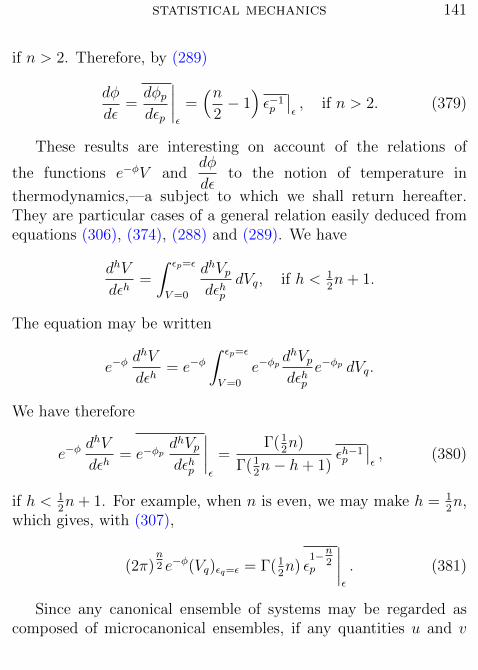
statistical mechanics 141
if n > 2. Therefore, by (289)
dφ
dε=dφpdεp
∣∣∣∣ε
=(n
2− 1)ε−1p
∣∣ε, if n > 2. (379)
These results are interesting on account of the relations of
the functions e−φV anddφ
dεto the notion of temperature in
thermodynamics,—a subject to which we shall return hereafter.They are particular cases of a general relation easily deduced fromequations (306), (374), (288) and (289). We have
dhV
dεh=
∫ εp=ε
V=0
dhVpdεhp
dVq, if h < 12n+ 1.
The equation may be written
e−φdhV
dεh= e−φ
∫ εp=ε
V=0
e−φpdhVpdεhp
e−φp dVq.
We have therefore
e−φdhV
dεh= e−φp
dhVpdεhp
∣∣∣∣ε
=Γ(1
2n)
Γ(12n− h+ 1)
εh−1p
∣∣ε, (380)
if h < 12n+ 1. For example, when n is even, we may make h = 1
2n,
which gives, with (307),
(2π)n2 e−φ(Vq)εq=ε = Γ(1
2n) ε
1−n2
p
∣∣∣∣ε
. (381)
Since any canonical ensemble of systems may be regarded ascomposed of microcanonical ensembles, if any quantities u and v

statistical mechanics 142
have the same average values in every microcanonical ensemble,they will have the same values in every canonical ensemble. Tobring equation (380) formally under this rule, we may observe thatthe first member being a function of ε is a constant value in amicrocanonical ensemble, and therefore identical with its averagevalue. We get thus the general equation
e−φdhV
dεh
∣∣∣∣Θ
= e−φpdhVpdεhp
∣∣∣∣Θ
=Γ(1
2n)
Γ(12n− h+ 1)
εh−1p
∣∣Θ
= Θ1−h,
(382)if h < 1
2n+ 1.∗ The equations
Θ = e−φV∣∣Θ
= e−φpVp∣∣Θ
=2
nεp |Θ , (383)
1
Θ=dφ
dε
∣∣∣∣Θ
=dφpdεp
∣∣∣∣Θ
=(n
2− 1)ε−1p
∣∣Θ, (384)
may be regarded as particular cases of the general equation. Thelast equation is subject to the condition that n > 2.
The last two equations give for a canonical ensemble, if n > 2,(1− 2
n
)εp |Θ ε−1
p
∣∣Θ
= 1. (385)
The corresponding equations for a microcanonical ensemble give, ifn > 2, (
1− 2
n
)εp |ε ε−1
p
∣∣ε
=dφ
d log V, (386)
which shows that dφ d log V approaches the value unity when n isvery great.
∗See equation (292).

statistical mechanics 143
If a system consists of two parts, having separate energies, wemay obtain equations similar in form to the preceding, which relateto the system as thus divided.∗ We shall distinguish quantitiesrelating to the parts by letters with suffixes, the same letters withoutsuffixes relating to the whole system. The extension-in-phase ofthe whole system within any given limits of the energies may berepresented by the double integral∫∫
dV1 dV2
taken within those limits, as appears at once from the definitionsof Chapter VIII. In an ensemble distributed with uniform densitywithin those limits, and zero density outside, the average value ofany function of ε1 and ε2 is given by the quotient∫∫
u dV1 dV2∫∫dV1 dV2
∗If this condition is rigorously fulfilled, the parts will have no influence oneach other, and the ensemble formed by distributing the whole microcanonicallyis too arbitrary a conception to have a real interest. The principal interest ofthe equations which we shall obtain will be in cases in which the condition isapproximately fulfilled. But for the purposes of a theoretical discussion, it isof course convenient to make such a condition absolute. Compare Chapter IV,pp. 39 ff., where a similar condition is considered in connection with canonicalensembles.

statistical mechanics 144
which may also be written∗∫∫u eφ1 dε dV2∫∫eφ1 dε dV2
.
If we make the limits of integration ε and ε+ dε, we get the averagevalue of u in an ensemble in which the whole system is microcanon-ically distributed in phase, viz.,
u |ε = e−φ∫ ε2=ε
V2=0
u eφ1 dV2, (387)
where φ1 and V2 are connected by the equation
ε1 + ε2 = constant = ε, (388)
and u, if given as function of ε1, or of ε1 and ε2, becomes in virtueof the same equation a function of ε2 alone.†
Thus
e−φ1V1
∣∣ε
= e−φ∫ ε2=ε
V2=0
V1 dV2, (389)
e−φV = e−φ1V1
∣∣ε
= e−φ2V2
∣∣ε. (390)
∗Where the analytical transformations are identical in form with those onthe preceding pages, it does not appear necessary to give all the steps with thesame detail.
†In the applications of the equation (387), we cannot obtain all the resultscorresponding to those which we have obtained from equation (374), becauseφp is a known function of εp, while φ1 must be treated as an arbitrary functionof ε1, or nearly so.

statistical mechanics 145
This requires a similar relation for canonical averages
Θ = e−φV∣∣Θ
= e−φ1V1
∣∣Θ
= e−φ2V2
∣∣Θ. (391)
Againdφ1
dε1
∣∣∣∣ε
= e−φ∫ ε2=ε
V2=0
dφ1
dε1eφ1 dV2. (392)
But if n1 > 2, eφ1 vanishes for V1 = 0,∗ and
d
dεeφ =
d
dε
∫ ε2=ε
V2=0
eφ1 dV2 =
∫ ε2=ε
V2=0
dφ1
dε1eφ1 dV2. (393)
Hence, if n1 > 2, and n2 > 2,
dφ
dε=dφ1
dε1
∣∣∣∣ε
=dφ2
dε2
∣∣∣∣ε
, (394)
and1
Θ=dφ
dε
∣∣∣∣Θ
=dφ1
dε1
∣∣∣∣Θ
=dφ2
dε2
∣∣∣∣Θ
. (395)
We have compared certain functions of the energy of the wholesystem with average values of similar functions of the kinetic energyof the whole system, and with average values of similar functions ofthe whole energy of a part of the system. We may also compare thesame functions with average values of the kinetic energy of a partof the system.
We shall express the total, kinetic, and potential energies ofthe whole system by ε, εp, and εq, and the kinetic energies of theparts by ε1p and ε2p. These kinetic energies are necessarily separate:we need not make any supposition concerning potential energies.
∗See Chapter VIII, equations (306) and (316).
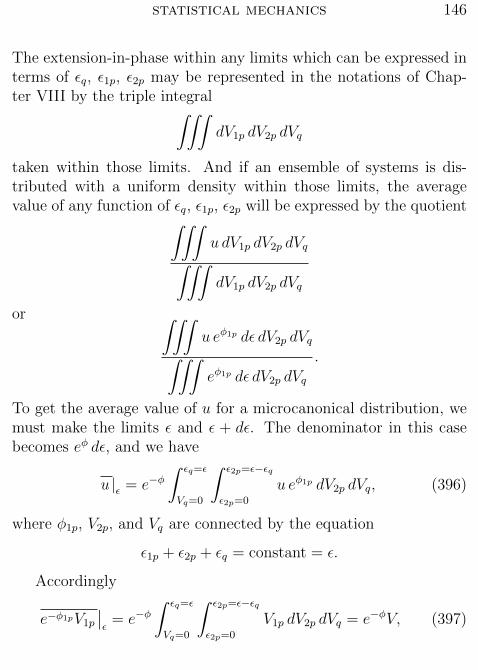
statistical mechanics 146
The extension-in-phase within any limits which can be expressed interms of εq, ε1p, ε2p may be represented in the notations of Chap-ter VIII by the triple integral∫∫∫
dV1p dV2p dVq
taken within those limits. And if an ensemble of systems is dis-tributed with a uniform density within those limits, the averagevalue of any function of εq, ε1p, ε2p will be expressed by the quotient∫∫∫
u dV1p dV2p dVq∫∫∫dV1p dV2p dVq
or ∫∫∫u eφ1p dε dV2p dVq∫∫∫eφ1p dε dV2p dVq
.
To get the average value of u for a microcanonical distribution, wemust make the limits ε and ε + dε. The denominator in this casebecomes eφ dε, and we have
u |ε = e−φ∫ εq=ε
Vq=0
∫ ε2p=ε−εq
ε2p=0
u eφ1p dV2p dVq, (396)
where φ1p, V2p, and Vq are connected by the equation
ε1p + ε2p + εq = constant = ε.
Accordingly
e−φ1pV1p
∣∣ε
= e−φ∫ εq=ε
Vq=0
∫ ε2p=ε−εq
ε2p=0
V1p dV2p dVq = e−φV, (397)

statistical mechanics 147
and we may write
e−φV = e−φ1pV1p
∣∣ε
= e−φ2pV2p
∣∣ε
=2
n1
ε1p |ε =2
n2
ε2p |ε , (398)
and
Θ = e−φV∣∣Θ
= e−φ1pV1p
∣∣Θ
= e−φ2pV2p
∣∣Θ
=2
n1
ε1p |Θ =2
n2
ε2p |Θ .(399)
Again, if n1 > 2,
dφ1p
dε1p
∣∣∣∣ε
= e−φ∫ εq=ε
Vq=0
∫ ε2p=ε−εq
ε2p=0
dφ1p
dε1peφ1p dV2p dVq
= e−φ∫ εq=ε
Vq=0
deφp
dεpdVq = e−φ
deφ
dε=dφ
dε. (400)
Hence, if n1 > 2, and n2 > 2,
dφ
dε=dφ1p
dε1p
∣∣∣∣ε
=dφ2p
dε2p
∣∣∣∣ε
= (12n1 − 1)ε−1
1p
∣∣ε
= (12n2 − 1)ε−1
2p
∣∣ε, (401)
1
Θ=dφ
dε
∣∣∣∣Θ
=dφ1p
dε1p
∣∣∣∣Θ
=dφ2p
dε2p
∣∣∣∣Θ
= (12n1 − 1)ε−1
1p
∣∣Θ
= (12n2 − 1)ε−1
2p
∣∣Θ.
(402)
We cannot apply the methods employed in the preceding pagesto the microcanonical averages of the (generalized) forces A1, A2,etc., exerted by a system on external bodies, since these quantitiesare not functions of the energies, either kinetic or potential, of thewhole or any part of the system. We may however use the methoddescribed on page 136.

statistical mechanics 148
Let us imagine an ensemble of systems distributed in phase ac-cording to the index of probability
c− (ε− ε′)2
ω2,
where ε′ is any constant which is a possible value of the energy,except only the least value which is consistent with the values ofthe external coordinates, and c and ω are other constants. We havetherefore ∫
all· · ·phases
∫ec−
(ε−ε′)2
ω2 dp1 . . . dqn = 1, (403)
or
e−c =
∫all· · ·
phases
∫e−
(ε−ε′)2
ω2 dp1 . . . dqn, (404)
or again
e−c =
∫ ε=∞
V=0
e−(ε−ε′)2
ω2 +φ dε. (405)
From (404) we have
de−c
da1
=
∫all· · ·
phases
∫2ε− ε′
ω2A1 e
−(ε−ε′)2
ω2 dp1 . . . dqn
=
∫ ε=∞
V=0
2ε− ε′
ω2A1 |ε e
−(ε−ε′)2
ω2 +φ dε, (406)
where A1 |ε denotes the average value of A1 in those systems of theensemble which have any same energy ε. (This is the same thing asthe average value of A1 in a microcanonical ensemble of energy ε.)The validity of the transformation is evident, if we consider sepa-rately the part of each integral which lies between two infinitesimally

statistical mechanics 149
differing limits of energy. Integrating by parts, we get
de−c
da1
= −[A1 |ε e
−(ε−ε′)2
ω2 +φ
]ε=∞V=0
+
∫ ε=∞
V=0
(dA1 |εdε
+ A1 |εdφ
dε
)e−
(ε−ε′)2
ω2 +φ dε. (407)
Differentiating (405), we get
de−c
da1
=
∫ ε=∞
V=0
dφ
da1
e−(ε−ε′)2
ω2 +φ dε−(e−
(ε−ε′)2
ω2 +φ dεαda1
)V=0
, (408)
where εα denotes the least value of ε consistent with the externalcoordinates. The last term in this equation represents the part ofde−c/da1 which is due to the variation of the lower limit of the in-tegral. It is evident that the expression in the brackets will vanishat the upper limit. At the lower limit, at which εp = 0, and εq hasthe least value consistent with the external coordinates, the averagesign on A1 |ε is superfluous, as there is but one value of A1 which isrepresented by −dεα/da1. Exceptions may indeed occur for partic-ular values of the external coordinates, at which dεα/da1 receive afinite increment, and the formula becomes illusory. Such particularvalues we may for the moment leave out of account. The last termof (408) is therefore equal to the first term of the second memberof (407). (We may observe that both vanish when n > 2 on accountof the factor eφ.)
We have therefore from these equations∫ ε=∞
V=0
(dA1 |εdε
+ A1 |εdφ
dε
)e−
(ε−ε′)2
ω2 +φ dε=
∫ ε=∞
V=0
dφ
da1
e−(ε−ε′)2
ω2 +φ dε,
or ∫ ε=∞
V=0
(dA1 |εdε
+ A1 |εdφ
dε− dφ
da1
)ec−
(ε−ε′)2
ω2 +φ dε = 0. (409)

statistical mechanics 150
That is: the average value in the ensemble of the quantity repre-sented by the principal parenthesis is zero. This must be true forany value of ω. If we diminish ω, the average value of the parenthe-sis at the limit when ω vanishes becomes identical with the valuefor ε = ε′. But this may be any value of the energy, except the leastpossible. We have therefore
dA1 |εdε
+ A1 |εdφ
dε− dφ
da1
= 0, (410)
unless it be for the least value of the energy consistent withthe external coordinates, or for particular values of the externalcoordinates. But the value of any term of this equation as de-termined for particular values of the energy and of the externalcoordinates is not distinguishable from its value as determined forvalues of the energy and external coordinates indefinitely near thoseparticular values. The equation therefore holds without limitation.Multiplying by eφ, we get
eφdA1 |εdε
+ A1 |ε eφ dφ
dε= eφ
dφ
da1
=deφ
da1
=d2V
da1 dε. (411)
The integral of this equation is
A1 |ε eφ =
dV
da1
+ F1, (412)
where F1 is a function of the external coordinates. We have anequation of this form for each of the external coordinates. Thisgives, with (266), for the complete value of the differential of V
dV = eφ dε+ (eφA1 |ε − F1) da1 + (eφA2 |ε − F2) da2 + etc., (413)

statistical mechanics 151
or
dV = eφ(dε+A1 |ε da1+A2 |ε da2+etc.)−F1 da1−F2 da2−etc. (414)
To determine the values of the functions F1, F2, etc., let us supposea1, a2, etc. to vary arbitrarily, while ε varies so as always to have theleast value consistent with the values of the external coordinates.This will make V = 0, and dV = 0. If n < 2, we shall have alsoeφ = 0, which will give
F1 = 0, F2 = 0, etc. (415)
The result is the same for any value of n. For in the variationsconsidered the kinetic energy will be constantly zero, and the po-tential energy will have the least value consistent with the externalcoordinates. The condition of the least possible potential energymay limit the ensemble at each instant to a single configuration, orit may not do so; but in any case the values of A1, A2, etc. will bethe same at each instant for all the systems of the ensemble,∗ andthe equation
dε+ A1 da1 + A2 da2 + etc. = 0
will hold for the variations considered. Hence the functions F1, F2,etc. vanish in any case, and we have the equation
dV = eφ dε+ eφA1 |ε da1 + eφA2 |ε da2 + etc., (416)
or
d log V =dε+ A1 |ε da1 + A2 |ε da2 + etc.
e−φV, (417)
∗This statement, as mentioned before, may have exceptions for particularvalues of the external coordinates. This will not invalidate the reasoning, whichhas to do with varying values of the external coordinates.

statistical mechanics 152
or again
dε = e−φV d log V − A1 |ε da1 − A2 |ε da2 − etc. (418)
It will be observed that the two last equations have the form of thefundamental differential equations of thermodynamics, e−φV corre-sponding to temperature and log V to entropy. We have alreadyobserved properties of e−φV suggestive of an analogy with temper-ature.∗ The significance of these facts will be discussed in anotherchapter.
The two last equations might be written more simply
dV =dε+ A1 |ε da1 + A2 |ε da2 + etc.
e−φ,
dε = e−φ dV − A1 |ε da1 − A2 |ε da2 − etc.,
and still have the form analogous to the thermodynamic equations,but e−φ has nothing like the analogies with temperature which wehave observed in e−φV .
∗See Chapter IX, page 131; also this chapter, page 140.

XI.
MAXIMUM AND MINIMUM PROPERTIES OF VARIOUSDISTRIBUTIONS IN PHASE.
In the following theorems we suppose, as always, that the systemsforming an ensemble are identical in nature and in the values of theexternal coordinates, which are here regarded as constants.
Theorem I. If an ensemble of systems is so distributed in phasethat the index of probability is a function of the energy, the averagevalue of the index is less than for any other distribution in whichthe distribution in energy is unaltered.
Let us write η for the index which is a function of the energy, andη + ∆η for any other which gives the same distribution in energy.It is to be proved that∫
all· · ·phases
∫(η + ∆η)eη+∆η dp1 . . . dqn >
∫all· · ·
phases
∫ηeη dp1 . . . dqn,
(419)where η is a function of the energy, and ∆η a function of the phase,which are subject to the conditions that∫
all· · ·phases
∫eη+∆η dp1 . . . dqn =
∫all· · ·
phases
∫eη dp1 . . . dqn = 1, (420)
and that for any value of the energy (ε′)∫ ε=ε′+dε′
ε=ε′· · ·∫eη+∆η dp1 . . . dqn =
∫ ε=ε′+dε′
ε=ε′· · ·∫eη dp1 . . . dqn. (421)
Equation (420) expresses the general relations which η and η+ ∆ηmust satisfy in order to be indices of any distributions, and
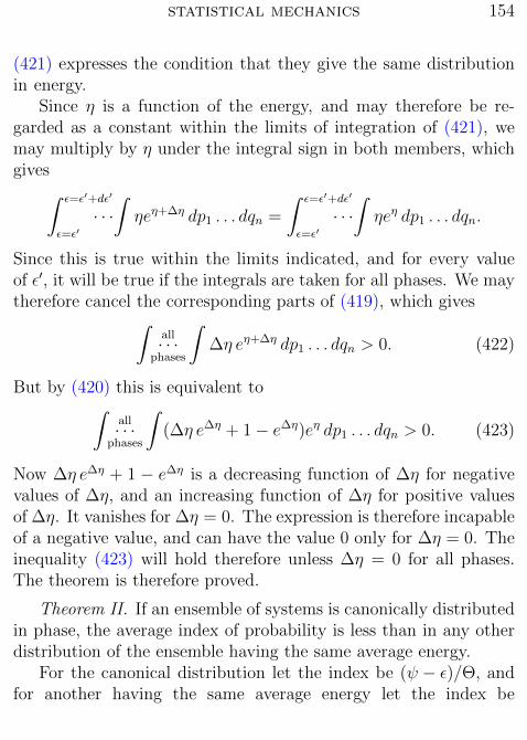
statistical mechanics 154
(421) expresses the condition that they give the same distributionin energy.
Since η is a function of the energy, and may therefore be re-garded as a constant within the limits of integration of (421), wemay multiply by η under the integral sign in both members, whichgives∫ ε=ε′+dε′
ε=ε′· · ·∫ηeη+∆η dp1 . . . dqn =
∫ ε=ε′+dε′
ε=ε′· · ·∫ηeη dp1 . . . dqn.
Since this is true within the limits indicated, and for every valueof ε′, it will be true if the integrals are taken for all phases. We maytherefore cancel the corresponding parts of (419), which gives∫
all· · ·phases
∫∆η eη+∆η dp1 . . . dqn > 0. (422)
But by (420) this is equivalent to∫all· · ·
phases
∫(∆η e∆η + 1− e∆η)eη dp1 . . . dqn > 0. (423)
Now ∆η e∆η + 1 − e∆η is a decreasing function of ∆η for negativevalues of ∆η, and an increasing function of ∆η for positive valuesof ∆η. It vanishes for ∆η = 0. The expression is therefore incapableof a negative value, and can have the value 0 only for ∆η = 0. Theinequality (423) will hold therefore unless ∆η = 0 for all phases.The theorem is therefore proved.
Theorem II. If an ensemble of systems is canonically distributedin phase, the average index of probability is less than in any otherdistribution of the ensemble having the same average energy.
For the canonical distribution let the index be (ψ − ε)/Θ, andfor another having the same average energy let the index be

statistical mechanics 155
(ψ − ε)/Θ + ∆η, where ∆η is an arbitrary function of the phasesubject only to the limitation involved in the notion of the index,that∫
all· · ·phases
∫eψ−εΘ
+∆η dp1 . . . dqn =
∫all· · ·
phases
∫eψ−εΘ dp1 . . . dqn = 1,
(424)and to that relating to the constant average energy, that∫
all· · ·phases
∫ε e
ψ−εΘ
+∆η dp1 . . . dqn =
∫all· · ·
phases
∫ε e
ψ−εΘ dp1 . . . dqn.
(425)It is to be proved that∫
all· · ·phases
∫ (ψ
Θ− ε
Θ+ ∆η
)eψ−εΘ
+∆η dp1 . . . dqn
>
∫all· · ·
phases
∫ (ψ
Θ− ε
Θ
)eψ−εΘ dp1 . . . dqn. (426)
Now in virtue of the first condition (424) we may cancel the constantterm ψ/Θ in the parentheses in (426), and in virtue of the secondcondition (425) we may cancel the term ε/Θ. The proposition to beproved is thus reduced to∫
all· · ·phases
∫∆η e
ψ−εΘ
+∆η dp1 . . . dqn > 0,
which may be written, in virtue of the condition (424),∫all· · ·
phases
∫(∆η e∆η + 1− e∆η)e
ψ−εΘ dp1 . . . dqn > 0. (427)
In this form its truth is evident for the same reasons which appliedto (423).

statistical mechanics 156
Theorem III. If Θ is any positive constant, the average valuein an ensemble of the expression η + ε/Θ (η denoting as usual theindex of probability and ε the energy) is less when the ensemble isdistributed canonically with modulus Θ, than for any other distri-bution whatever.
In accordance with our usual notation let us write (ψ− ε)/Θ forthe index of the canonical distribution. In any other distributionlet the index be (ψ − ε)/Θ + ∆η.
In the canonical ensemble η + ε/Θ has the constant value ψ/Θ;in the other ensemble it has the value ψ/Θ + ∆η. The propositionto be proved may therefore be written
ψ
Θ<
∫all· · ·
phases
∫ (ψ
Θ+ ∆η
)eψ−εΘ
+∆η dp1 . . . dqn, (428)
where∫all· · ·
phases
∫eψ−εΘ
+∆η dp1 . . . dqn =
∫all· · ·
phases
∫eψ−εΘ dp1 . . . dqn = 1.
(429)In virtue of this condition, since ψ/Θ is constant, the propositionto be proved reduces to
0 <
∫all· · ·
phases
∫∆η e
ψ−εΘ
+∆η dp1 . . . dqn, (430)
where the demonstration may be concluded as in the last theorem.If we should substitute for the energy in the preceding theorems
any other function of the phase, the theorems, mutatis mutandis,would still hold. On account of the unique importance of the energyas a function of the phase, the theorems as given are especiallyworthy of notice. When the case is such that other functions of thephase have important properties relating to statistical equilibrium,

statistical mechanics 157
as described in Chapter IV,∗ the three following theorems, which aregeneralizations of the preceding, may be useful. It will be sufficientto give them without demonstration, as the principles involved arein no respect different.
Theorem IV. If an ensemble of systems is so distributed in phasethat the index of probability is any function of F1, F2, etc., (theseletters denoting functions of the phase,) the average value of theindex is less than for any other distribution in phase in which thedistribution with respect to the functions F1, F2, etc. is unchanged.
Theorem V. If an ensemble of systems is so distributed in phasethat the index of probability is a linear function of F1, F2, etc.,(these letters denoting functions of the phase,) the average valueof the index is less than for any other distribution in which thefunctions F1, F2, etc. have the same average values.
Theorem VI. The average value in an ensemble of systems ofη+F (where η denotes as usual the index of probability and F anyfunction of the phase) is less when the ensemble is so distributedthat η + F is constant than for any other distribution whatever.
Theorem VII. If a system which in its different phases consti-tutes an ensemble consists of two parts, and we consider the averageindex of probability for the whole system, and also the average in-dices for each of the parts taken separately, the sum of the averageindices for the parts will be either less than the average index for thewhole system, or equal to it, but cannot be greater. The limitingcase of equality occurs when the distribution in phase of each partis independent of that of the other, and only in this case.
Let the coordinates and momenta of the whole system beq1, . . . qn, p1, . . . pn, of which q1, . . . qm, p1, . . . pm relate to one
∗See pages 41–46.

statistical mechanics 158
part of the system, and qm+1, . . . qn, pm+1, . . . pn to the other. Ifthe index of probability for the whole system is denoted by η, theprobability that the phase of an unspecified system lies within anygiven limits is expressed by the integral∫
· · ·∫eη dp1 . . . dqn (431)
taken for those limits. If we set∫· · ·∫eη dpm+1 . . . dpn dqm+1 . . . dqn = eη1 , (432)
where the integrations cover all phases of the second system, and∫· · ·∫eη dp1 . . . dpm dq1 . . . dqm = eη2 , (433)
where the integrations cover all phases of the first system, the inte-gral (431) will reduce to the form∫
· · ·∫eη1 dp1 . . . dpm dq1 . . . dqm, (434)
when the limits can be expressed in terms of the coordinates andmomenta of the first part of the system. The same integral willreduce to ∫
· · ·∫eη2 dpm+1 . . . dpn dqm+1 . . . dqn, (435)
when the limits can be expressed in terms of the coordinates andmomenta of the second part of the system. It is evident that η1 andη2 are the indices of probability for the two parts of the systemtaken separately.

statistical mechanics 159
The main proposition to be proved may be written∫· · ·∫η1e
η1 dp1 . . . dqm +
∫· · ·∫η2e
η2 dpm+1 . . . dqn
≤∫· · ·∫ηeη dp1 . . . dqn, (436)
where the first integral is to be taken over all phases of the firstpart of the system, the second integral over all phases of the secondpart of the system, and the last integral over all phases of the wholesystem. Now we have∫
· · ·∫eη dp1 . . . dqn = 1, (437)∫
· · ·∫eη1 dp1 . . . dqm = 1, (438)
and ∫· · ·∫eη2 dpm+1 . . . dqn = 1, (439)
where the limits cover in each case all the phases to which thevariables relate. The two last equations, which are in themselvesevident, may be derived by partial integration from the first.
It appears from the definitions of η1 and η2 that (436) may alsobe written∫· · ·∫η1e
η dp1 . . . dqn +
∫· · ·∫η2e
η dp1 . . . dqn
≤∫· · ·∫ηeη dp1 . . . dqn, (440)

statistical mechanics 160
or ∫· · ·∫
(η − η1 − η2)eη dp1 . . . dqn ≥ 0,
where the integrations cover all phases. Adding the equation∫· · ·∫eη1+η2 dp1 . . . dqn = 1, (441)
which we get by multiplying (438) and (439), and subtracting (437),we have for the proposition to be proved∫
all· · ·phases
∫ [(η − η1 − η2)eη + eη1+η2 − eη
]dp1 . . . dqn ≥ 0. (442)
Letu = η − η1 − η2. (443)
The main proposition to be proved may be written∫all· · ·
phases
∫(u eu + 1− eu)eη1+η2 dp1 . . . dqn ≥ 0. (444)
This is evidently true since the quantity in the parenthesis is inca-pable of a negative value.∗ Moreover the sign = can hold only whenthe quantity in the parenthesis vanishes for all phases, i.e., whenu = 0 for all phases. This makes η = η1 + η2 for all phases, whichis the analytical condition which expresses that the distributions inphase of the two parts of the system are independent.
Theorem VIII. If two or more ensembles of systems which areidentical in nature, but may be distributed differently in phase, areunited to form a single ensemble, so that the probability-coefficient
∗See Theorem I, where this is proved of a similar expression.

statistical mechanics 161
of the resulting ensemble is a linear function of the probability-coefficients of the original ensembles, the average index of proba-bility of the resulting ensemble cannot be greater than the samelinear function of the average indices of the original ensembles. Itcan be equal to it only when the original ensembles are similarlydistributed in phase.
Let P1, P2, etc. be the probability-coefficients of the original en-sembles, and P that of the ensemble formed by combining them;and let N1, N2, etc. be the numbers of systems in the original en-sembles. It is evident that we shall have
P = c1P1 + c2P2 + etc. =∑
(c1P1), (445)
where
c1 =N1∑N1
, c2 =N2∑N1
, etc. (446)
The main proposition to be proved is that∫all· · ·
phases
∫P logP dp1 . . . dqn ≤
∑[c1
∫all· · ·
phases
∫P1 logP1 dp1 . . . dqn
](447)
or ∫all· · ·
phases
∫ [∑(c1P1 logP1)− P logP
]dp1 . . . dqn ≥ 0. (448)
If we set
Q1 = P1 logP1 − P1 logP − P1 + P
Q1 will be positive, except when it vanishes for P1 = P . To provethis, we may regard P1 and P as any positive quantities. Then(
dQ1
dP1
)P
= logP1 − logP,

statistical mechanics 162
(d2Q1
dP 21
)P
=1
P1
.
Since Q1 and dQ1/dP1 vanish for P1 = P , and the seconddifferential coefficient is always positive, Q1 must be positive exceptwhen P1 = P . Therefore, if Q2, etc. have similar definitions,∑
(c1Q1) ≥ 0. (449)
But since ∑(c1P1) = P
and ∑c1 = 1,∑
(c1Q1) =∑
(c1P1 logP1)− P logP. (450)
This proves (448), and shows that the sign = will hold only when
P1 = P, P2 = P, etc.
for all phases, i.e., only when the distribution in phase of the originalensembles are all identical.
Theorem IX. A uniform distribution of a given number of sys-tems within given limits of phase gives a less average index of prob-ability of phase than any other distribution.
Let η be the constant index of the uniform distribution, andη + ∆η the index of some other distribution. Since the number ofsystems within the given limits is the same in the two distributionswe have∫
· · ·∫eη+∆η dp1 . . . dqn =
∫· · ·∫eη dp1 . . . dqn, (451)

statistical mechanics 163
where the integrations, like those which follow, are to be takenwithin the given limits. The proposition to be proved may be writ-ten∫· · ·∫
(η + ∆η)eη+∆η dp1 . . . dqn >
∫· · ·∫ηeη dp1 . . . dqn, (452)
or, since η is constant,∫· · ·∫
(η + ∆η)e∆η dp1 . . . dqn >
∫· · ·∫η dp1 . . . dqn. (453)
In (451) also we may cancel the constant factor eη, and multiply bythe constant factor (η + 1). This gives∫
· · ·∫
(η + 1)e∆η dp1 . . . dqn =
∫· · ·∫
(η + 1) dp1 . . . dqn.
The subtraction of this equation will not alter the inequality to beproved, which may therefore be written∫
· · ·∫
(∆η − 1)e∆η dp1 . . . dqn >
∫· · ·∫−dp1 . . . dqn
or ∫· · ·∫
(∆ηe∆η − e∆η + 1) dp1 . . . dqn > 0. (454)
Since the parenthesis in this expression represents a positive value,except when it vanishes for ∆η = 0, the integral will be positive un-less ∆η vanishes everywhere within the limits, which would makethe difference of the two distributions vanish. The theorem is there-fore proved.

XII.
ON THE MOTION OF SYSTEMS AND ENSEMBLES OFSYSTEMS THROUGH LONG PERIODS OF TIME.
An important question which suggests itself in regard to any caseof dynamical motion is whether the system considered will returnin the course of time to its initial phase, or, if it will not returnexactly to that phase, whether it will do so to any required degreeof approximation in the course of a sufficiently long time. To beable to give even a partial answer to such questions, we must knowsomething in regard to the dynamical nature of the system. In thefollowing theorem, the only assumption in this respect is such as wehave found necessary for the existence of the canonical distribution.
If we imagine an ensemble of identical systems to be distributedwith a uniform density throughout any finite extension-in-phase,the number of the systems which leave the extension-in-phase andwill not return to it in the course of time is less than any assignablefraction of the whole number; provided, that the total extension-in-phase for the systems considered between two limiting values of theenergy is finite, these limiting values being less and greater respec-tively than any of the energies of the first-mentioned extension-in-phase.
To prove this, we observe that at the moment which we call ini-tial the systems occupy the given extension-in-phase. It is evidentthat some systems must leave the extension immediately, unless allremain in it forever. Those systems which leave the extension atthe first instant, we shall call the front of the ensemble. It willbe convenient to speak of this front as generating the extension-in-phase through which it passes in the course of time, as in geometrya surface is said to generate the volume through which it passes. In

statistical mechanics 165
equal times the front generates equal extensions in phase. This is animmediate consequence of the principle of conservation of extension-in-phase, unless indeed we prefer to consider it as a slight variationin the expression of that principle. For in two equal short intervalsof time let the extensions generated be A and B. (We make theintervals short simply to avoid the complications in the enunciationor interpretation of the principle which would arise when the sameextension-in-phase is generated more than once in the interval con-sidered.) Now if we imagine that at a given instant systems aredistributed throughout the extension A, it is evident that the samesystems will after a certain time occupy the extension B, whichis therefore equal to A in virtue of the principle cited. The frontof the ensemble, therefore, goes on generating equal extensions inequal times. But these extensions are included in a finite extension,viz., that bounded by certain limiting values of the energy. Sooneror later, therefore, the front must generate phases which it has be-fore generated. Such second generation of the same phases mustcommence with the initial phases. Therefore a portion at least ofthe front must return to the original extension-in-phase. The sameis of course true of the portion of the ensemble which follows thatportion of the front through the same phases at a later time.
It remains to consider how large the portion of the ensemble is,which will return to the original extension-in-phase. There can beno portion of the given extension-in-phase, the systems of whichleave the extension and do not return. For we can prove for anyportion of the extension as for the whole, that at least a portion ofthe systems leaving it will return.
We may divide the given extension-in-phase into parts as follows.There may be parts such that the systems within them will neverpass out of them. These parts may indeed constitute the whole of

statistical mechanics 166
the given extension. But if the given extension is very small, theseparts will in general be non-*existent. There may be parts suchthat systems within them will all pass out of the given extensionand all return within it. The whole of the given extension-in-phaseis made up of parts of these two kinds. This does not exclude thepossibility of phases on the boundaries of such parts, such thatsystems starting with those phases would leave the extension andnever return. But in the supposed distribution of an ensemble ofsystems with a uniform density-in-phase, such systems would notconstitute any assignable fraction of the whole number.
These distinctions may be illustrated by a very simple example.If we consider the motion of a rigid body of which one point isfixed, and which is subject to no forces, we find three cases. (1) Themotion is periodic. (2) The system will never return to its originalphase, but will return infinitely near to it. (3) The system will neverreturn either exactly or approximately to its original phase. But ifwe consider any extension-in-phase, however small, a system leavingthat extension will return to it except in the case called by Poinsot‘singular,’ viz., when the motion is a rotation about an axis lying inone of two planes having a fixed position relative to the rigid body.But all such phases do not constitute any true extension-in-phasein the sense in which we have defined and used the term.∗
∗An ensemble of systems distributed in phase is a less simple and elementaryconception than a single system. But by the consideration of suitable ensemblesinstead of single systems, we may get rid of the inconvenience of having to con-sider exceptions formed by particular cases of the integral equations of motion,these cases simply disappearing when the ensemble is substituted for the singlesystem as a subject of study. This is especially true when the ensemble is dis-tributed, as in the case called canonical, throughout an extension-in-phase. Ina less degree it is true of the microcanonical ensemble, which does not occupyany extension-in-phase, (in the sense in which we have used the term,) although

statistical mechanics 167
In the same way it may be proved that the systems in a canonicalensemble which at a given instant are contained within any finiteextension-in-phase will in general return to that extension-in-phase,if they leave it, the exceptions, i.e., the number which pass out ofthe extension-in-phase and do not return to it, being less than anyassignable fraction of the whole number. In other words, the prob-ability that a system taken at random from the part of a canonicalensemble which is contained within any given extension-in-phase,will pass out of that extension and not return to it, is zero.
A similar theorem may be enunciated with respect to a micro-canonical ensemble. Let us consider the fractional part of such anensemble which lies within any given limits of phase. This fractionwe shall denote by F . It is evidently constant in time since the en-semble is in statistical equilibrium. The systems within the limitswill not in general remain the same, but some will pass out in eachunit of time while an equal number come in. Some may pass outnever to return within the limits. But the number which in any timehowever long pass out of the limits never to return will not bear anyfinite ratio to the number within the limits at a given instant. For,if it were otherwise, let f denote the fraction representing such ratiofor the time T . Then, in the time T , the number which pass outnever to return will bear the ratio fF to the whole number in theensemble, and in a time exceeding T/(fF ) the number which passout of the limits never to return would exceed the total number ofsystems in the ensemble. The proposition is therefore proved.
This proof will apply to the cases before considered, and may beregarded as more simple than that which was given. It may also be
it is convenient to regard it as a limiting case with respect to ensembles whichdo, as we thus gain for the subject some part of the analytical simplicity whichbelongs to the theory of ensembles which occupy true extensions-in-phase.

statistical mechanics 168
applied to any true case of statistical equilibrium. By a true case ofstatistical equilibrium is meant such as may be described by givingthe general value of the probability that an unspecified system ofthe ensemble is contained within any given limits of phase.∗
∗An ensemble in which the systems are material points constrained to movein vertical circles, with just enough energy to carry them to the highest points,cannot afford a true example of statistical equilibrium. For any other value ofthe energy than the critical value mentioned, we might in various ways describean ensemble in statistical equilibrium, while the same language applied to thecritical value of the energy would fail to do so. Thus, if we should say that theensemble is so distributed that the probability that a system is in any givenpart of the circle is proportioned to the time which a single system spends inthat part, motion in either direction being equally probable, we should perfectlydefine a distribution in statistical equilibrium for any value of the energy exceptthe critical value mentioned above, but for this value of the energy all theprobabilities in question would vanish unless the highest point is included inthe part of the circle considered, in which case the probability is unity, or formsone of its limits, in which case the probability is indeterminate. Compare thefoot-note on page 139.
A still more simple example is afforded by the uniform motion of a materialpoint in a straight line. Here the impossibility of statistical equilibrium is notlimited to any particular energy, and the canonical distribution as well as themicrocanonical is impossible.
These examples are mentioned here in order to show the necessity of cautionin the application of the above principle, with respect to the question whetherwe have to do with a true case of statistical equilibrium.
Another point in respect to which caution must be exercised is that the partof an ensemble of which the theorem of the return of systems is asserted shouldbe entirely defined by limits within which it is contained, and not by any suchcondition as that a certain function of phase shall have a given value. This isnecessary in order that the part of the ensemble which is considered should beany assignable fraction of the whole. Thus, if we have a canonical ensembleconsisting of material points in vertical circles, the theorem of the return ofsystems may be applied to a part of the ensemble defined as contained in agiven part of the circle. But it may not be applied in all cases to a part of the

statistical mechanics 169
Let us next consider whether an ensemble of isolated systemshas any tendency in the course of time toward a state of statisticalequilibrium.
There are certain functions of phase which are constant in time.The distribution of the ensemble with respect to the values of thesefunctions is necessarily invariable, that is, the number of systemswithin any limits which can be specified in terms of these functionscannot vary in the course of time. The distribution in phase whichwithout violating this condition gives the least value of the averageindex of probability of phase (η) is unique, and is that in which theindex of probability (η) is a function of the functions mentioned.∗
It is therefore a permanent distribution,† and the only permanentdistribution consistent with the invariability of the distribution withrespect to the functions of phase which are constant in time.
It would seem, therefore, that we might find a sort of measureof the deviation of an ensemble from statistical equilibrium in theexcess of the average index above the minimum which is consistentwith the condition of the invariability of the distribution with re-spect to the constant functions of phase. But we have seen that theindex of probability is constant in time for each system of the en-semble. The average index is therefore constant, and we find by thismethod no approach toward statistical equilibrium in the course oftime.
Yet we must here exercise great caution. One function mayapproach indefinitely near to another function, while some quan-
ensemble defined as contained in a given part of the circle and having a givenenergy. It would, in fact, express the exact opposite of the truth when the givenenergy is the critical value mentioned above.
∗See Chapter XI, Theorem IV.†See Chapter IV, sub init.

statistical mechanics 170
tity determined by the first does not approach the correspondingquantity determined by the second. A line joining two points mayapproach indefinitely near to the straight line joining them, whileits length remains constant. We may find a closer analogy with thecase under consideration in the effect of stirring an incompressibleliquid.∗ In space of 2n dimensions the case might be made analyt-ically identical with that of an ensemble of systems of n degrees offreedom, but the analogy is perfect in ordinary space. Let us sup-pose the liquid to contain a certain amount of coloring matter whichdoes not affect its hydrodynamic properties. Now the state in whichthe density of the coloring matter is uniform, i.e., the state of per-fect mixture, which is a sort of state of equilibrium in this respectthat the distribution of the coloring matter in space is not affectedby the internal motions of the liquid, is characterized by a minimumvalue of the average square of the density of the coloring matter.Let us suppose, however, that the coloring matter is distributedwith a variable density. If we give the liquid any motion whatever,subject only to the hydrodynamic law of incompressibility,—it maybe a steady flux, or it may vary with the time,—the density of thecoloring matter at any same point of the liquid will be unchanged,and the average square of this density will therefore be unchanged.Yet no fact is more familiar to us than that stirring tends to bringa liquid to a state of uniform mixture, or uniform densities of itscomponents, which is characterized by minimum values of the av-erage squares of these densities. It is quite true that in the physicalexperiment the result is hastened by the process of diffusion, butthe result is evidently not dependent on that process.
∗By liquid is here meant the continuous body of theoretical hydrodynamics,and not anything of the molecular structure and molecular motions of realliquids.

statistical mechanics 171
The contradiction is to be traced to the notion of the densityof the coloring matter, and the process by which this quantity isevaluated. This quantity is the limiting ratio of the quantity ofthe coloring matter in an element of space to the volume of thatelement. Now if we should take for our elements of volume, afterany amount of stirring, the spaces occupied by the same portions ofthe liquid which originally occupied any given system of elements ofvolume, the densities of the coloring matter, thus estimated, wouldbe identical with the original densities as determined by the givensystem of elements of volume. Moreover, if at the end of any finiteamount of stirring we should take our elements of volume in any or-dinary form but sufficiently small, the average square of the densityof the coloring matter, as determined by such element of volume,would approximate to any required degree to its value before thestirring. But if we take any element of space of fixed position anddimensions, we may continue the stirring so long that the densitiesof the colored liquid estimated for these fixed elements will approacha uniform limit, viz., that of perfect mixture.
The case is evidently one of those in which the limit of a limithas different values, according to the order in which we apply theprocesses of taking a limit. If treating the elements of volume asconstant, we continue the stirring indefinitely, we get a uniformdensity, a result not affected by making the elements as small aswe choose; but if treating the amount of stirring as finite, we di-minish indefinitely the elements of volume, we get exactly the samedistribution in density as before the stirring, a result which is not af-fected by continuing the stirring as long as we choose. The questionis largely one of language and definition. One may perhaps be al-lowed to say that a finite amount of stirring will not affect the meansquare of the density of the coloring matter, but an infinite amount

statistical mechanics 172
of stirring may be regarded as producing a condition in which themean square of the density has its minimum value, and the densityis uniform. We may certainly say that a sensibly uniform density ofthe colored component may be produced by stirring. Whether thetime required for this result would be long or short depends uponthe nature of the motion given to the liquid, and the fineness of ourmethod of evaluating the density.
All this may appear more distinctly if we consider a special caseof liquid motion. Let us imagine a cylindrical mass of liquid ofwhich one sector of 90 is black and the rest white. Let it havea motion of rotation about the axis of the cylinder in which theangular velocity is a function of the distance from the axis. In thecourse of time the black and the white parts would become drawnout into thin ribbons, which would be wound spirally about the axis.The thickness of these ribbons would diminish without limit, andthe liquid would therefore tend toward a state of perfect mixtureof the black and white portions. That is, in any given elementof space, the proportion of the black and white would approach1 : 3 as a limit. Yet after any finite time, the total volume would bedivided into two parts, one of which would consist of the white liquidexclusively, and the other of the black exclusively. If the coloringmatter, instead of being distributed initially with a uniform densitythroughout a section of the cylinder, were distributed with a densityrepresented by any arbitrary function of the cylindrical coordinatesr, θ and z, the effect of the same motion continued indefinitely wouldbe an approach to a condition in which the density is a function ofr and z alone. In this limiting condition, the average square ofthe density would be less than in the original condition, when thedensity was supposed to vary with θ, although after any finite timethe average square of the density would be the same as at first.

statistical mechanics 173
If we limit our attention to the motion in a single plane per-pendicular to the axis of the cylinder, we have something which isalmost identical with a diagrammatic representation of the changesin distribution in phase of an ensemble of systems of one degree offreedom, in which the motion is periodic, the period varying withthe energy, as in the case of a pendulum swinging in a circulararc. If the coordinates and momenta of the systems are representedby rectangular coordinates in the diagram, the points in the di-agram representing the changing phases of moving systems, willmove about the origin in closed curves of constant energy. The mo-tion will be such that areas bounded by points representing movingsystems will be preserved. The only difference between the motionof the liquid and the motion in the diagram is that in one case thepaths are circular, and in the other they differ more or less fromthat form.
When the energy is proportional to p2+q2 the curves of constantenergy are circles, and the period is independent of the energy.There is then no tendency toward a state of statistical equilibrium.The diagram turns about the origin without change of form. Thiscorresponds to the case of liquid motion, when the liquid revolveswith a uniform angular velocity like a rigid solid.
The analogy between the motion of an ensemble of systems inan extension-in-phase and a steady current in an incompressible liq-uid, and the diagrammatic representation of the case of one degreeof freedom, which appeals to our geometrical intuitions, may besufficient to show how the conservation of density-in-phase, whichinvolves the conservation of the average value of the index of proba-bility of phase, is consistent with an approach to a limiting conditionin which that average value is less. We might perhaps fairly inferfrom such considerations as have been adduced that an approach

statistical mechanics 174
to a limiting condition of statistical equilibrium is the general rule,when the initial condition is not of that character. But the sub-ject is of such importance that it seems desirable to give it fartherconsideration.
Let us suppose that the total extension-in-phase for the kind ofsystem considered to be divided into equal elements (DV ) whichare very small but not infinitely small. Let us imagine an ensembleof systems distributed in this extension in a manner representedby the index of probability η, which is an arbitrary function of thephase subject only to the restriction expressed by equation (46) ofChapter I. We shall suppose the elements DV to be so small thatη may in general be regarded as sensibly constant within any oneof them at the initial moment. Let the path of a system be definedas the series of phases through which it passes.
At the initial moment (t′) a certain system is in an element ofextension DV ′. Subsequently, at the time t′′, the same system isin the element DV ′′. Other systems which were at first in DV ′
will at the time t′′ be in DV ′′, but not all, probably. The systemswhich were at first in DV ′ will at the time t′′ occupy an extension-in-phase exactly as large as at first. But it will probably be distributedamong a very great number of the elements (DV ) into which we havedivided the total extension-in-phase. If it is not so, we can generallytake a later time at which it will be so. There will be exceptions tothis for particular laws of motion, but we will confine ourselves towhat may fairly be called the general case. Only a very small partof the systems initially in DV ′ will be found in DV ′′ at the time t′′,and those which are found in DV ′′ at that time were at the initialmoment distributed among a very large number of elements DV .
What is important for our purpose is the value of η, the indexof probability of phase in the element DV ′′ at the time t′′. In the

statistical mechanics 175
part of DV ′′ occupied by systems which at the time t′ were in DV ′
the value of η will be the same as its value in DV ′ at the time t′,which we shall call η′. In the parts of DV ′′ occupied by systemswhich at t′ were in elements very near to DV ′ we may suppose thevalue of η to vary little from η′. We cannot assume this in regardto parts of DV ′′ occupied by systems which at t′ were in elementsremote from DV ′. We want, therefore, some idea of the nature ofthe extension-in-phase occupied at t′ by the systems which at t′′ willoccupy DV ′′. Analytically, the problem is identical with finding theextension occupied at t′′ by the systems which at t′ occupied DV ′.Now the systems in DV ′′ which lie on the same path as the systemfirst considered, evidently arrived at DV ′′ at nearly the same time,and must have left DV ′ at nearly the same time, and therefore at t′
were in or near DV ′. We may therefore take η′ as the value for thesesystems. The same essentially is true of systems in DV ′′ which lie onpaths very close to the path already considered. But with respectto paths passing through DV ′ and DV ′′, but not so close to thefirst path, we cannot assume that the time required to pass fromDV ′ to DV ′′ is nearly the same as for the first path. The differenceof the times required may be small in comparison with t′′ − t′, butas this interval can be as large as we choose, the difference of thetimes required in the different paths has no limit to its possiblevalue. Now if the case were one of statistical equilibrium, the valueof η would be constant in any path, and if all the paths whichpass through DV ′′ also pass through or near DV ′, the value of ηthroughout DV ′′ will vary little from η′. But when the case is notone of statistical equilibrium, we cannot draw any such conclusion.The only conclusion which we can draw with respect to the phaseat t′ of the systems which at t′′ are in DV ′′ is that they are nearlyon the same path.
statistical mechanics 176
Now if we should make a new estimate of indices of probability ofphase at the time t′′, using for this purpose the elements DV ,—thatis, if we should divide the number of systems in DV ′′, for example,by the total number of systems, and also by the extension-in-phaseof the element, and take the logarithm of the quotient, we wouldget a number which would be less than the average value of η forthe systems within DV ′′ based on the distribution in phase at thetime t′.∗ Hence the average value of η for the whole ensemble ofsystems based on the distribution at t′′ will be less than the averagevalue based on the distribution at t′.
We must not forget that there are exceptions to this general rule.These exceptions are in cases in which the laws of motion are suchthat systems having small differences of phase will continue alwaysto have small differences of phase.
It is to be observed that if the average index of probability inan ensemble may be said in some sense to have a less value at onetime than at another, it is not necessarily priority in time whichdetermines the greater average index. If a distribution, which is notone of statistical equilibrium, should be given for a time t′, and thedistribution at an earlier time t′′ should be defined as that givenby the corresponding phases, if we increase the interval leaving t′
fixed and taking t′′ at an earlier and earlier date, the distributionat t′′ will in general approach a limiting distribution which is instatistical equilibrium. The determining difference in such cases isthat between a definite distribution at a definite time and the limitof a varying distribution when the moment considered is carriedeither forward or backward indefinitely.†
∗See Chapter XI, Theorem IX.†One may compare the kinematical truism that when two points are moving
with uniform velocities, (with the single exception of the case where the relative

statistical mechanics 177
But while the distinction of prior and subsequent events may beimmaterial with respect to mathematical fictions, it is quite other-wise with respect to the events of the real world. It should not beforgotten, when our ensembles are chosen to illustrate the proba-bilities of events in the real world, that while the probabilities ofsubsequent events may often be determined from the probabilitiesof prior events, it is rarely the case that probabilities of prior eventscan be determined from those of subsequent events, for we are rarelyjustified in excluding the consideration of the antecedent probabilityof the prior events.
It is worthy of notice that to take a system at random froman ensemble at a date chosen at random from several given dates,t′, t′′, etc., is practically the same thing as to take a system atrandom from the ensemble composed of all the systems of the givenensemble in their phases at the time t′, together with the samesystems in their phases at the time t′′, etc. By Theorem VIII ofChapter XI this will give an ensemble in which the average indexof probability will be less than in the given ensemble, except in thecase when the distribution in the given ensemble is the same atthe times t′, t′′, etc. Consequently, any indefiniteness in the timein which we take a system at random from an ensemble has thepractical effect of diminishing the average index of the ensemblefrom which the system may be supposed to be drawn, except whenthe given ensemble is in statistical equilibrium.
motion is zero,) their mutual distance at any definite time is less than for t =∞,or t = −∞.

XIII.
EFFECT OF VARIOUS PROCESSES ON AN ENSEMBLE OFSYSTEMS.
In the last chapter and in Chapter I we have considered the changeswhich take place in the course of time in an ensemble of isolatedsystems. Let us now proceed to consider the changes which will takeplace in an ensemble of systems under external influences. These ex-ternal influences will be of two kinds, the variation of the coordinateswhich we have called external, and the action of other ensembles ofsystems. The essential difference of the two kinds of influence con-sists in this, that the bodies to which the external coordinates relateare not distributed in phase, while in the case of interaction of thesystems of two ensembles, we have to regard the fact that both aredistributed in phase. To find the effect produced on the ensem-ble with which we are principally concerned, we have therefore toconsider single values of what we have called external coordinates,but an infinity of values of the internal coordinates of any otherensemble with which there is interaction.
Or,—to regard the subject from another point of view,—the ac-tion between an unspecified system of an ensemble and the bodiesrepresented by the external coordinates, is the action between a sys-tem imperfectly determined with respect to phase and one which isperfectly determined; while the interaction between two unspecifiedsystems belonging to different ensembles is the action between twosystems both of which are imperfectly determined with respect tophase.∗
∗In the development of the subject, we shall find that this distinction corre-sponds to the distinction in thermodynamics between mechanical and thermalaction.

statistical mechanics 179
We shall suppose the ensembles which we consider to be dis-tributed in phase in the manner described in Chapter I, andrepresented by the notations of that chapter, especially by theindex of probability of phase (η). There are therefore 2n inde-pendent variations in the phases which constitute the ensemblesconsidered. This excludes ensembles like the microcanonical, inwhich, as energy is constant, there are only 2n − 1 independentvariations of phase. This seems necessary for the purposes of ageneral discussion. For although we may imagine a microcanon-ical ensemble to have a permanent existence when isolated fromexternal influences, the effect of such influences would generallybe to destroy the uniformity of energy in the ensemble. Moreover,since the microcanonical ensemble may be regarded as a limitingcase of such ensembles as are described in Chapter I, (and thatin more than one way, as shown in Chapter X,) the exclusion israther formal than real, since any properties which belong to themicrocanonical ensemble could easily be derived from those of theensembles of Chapter I, which in a certain sense may be regardedas representing the general case.
Let us first consider the effect of variation of the externalcoordinates. We have already had occasion to regard these quan-tities as variable in the differentiation of certain equations relatingto ensembles distributed according to certain laws called canonicalor microcanonical. That variation of the external coordinates was,however, only carrying the attention of the mind from an ensemblewith certain values of the external coordinates, and distributedin phase according to some general law depending upon thosevalues, to another ensemble with different values of the externalcoordinates, and with the distribution changed to conform to thesenew values.

statistical mechanics 180
What we have now to consider is the effect which would actuallyresult in the course of time in an ensemble of systems in whichthe external coordinates should be varied in any arbitrary manner.Let us suppose, in the first place, that these coordinates are variedabruptly at a given instant, being constant both before and afterthat instant. By the definition of the external coordinates it appearsthat this variation does not affect the phase of any system of theensemble at the time when it takes place. Therefore it does notaffect the index of probability of phase (η) of any system, or theaverage value of the index (η) at that time. And if these quantitiesare constant in time before the variation of the external coordinates,and after that variation, their constancy in time is not interruptedby that variation. In fact, in the demonstration of the conservationof probability of phase in Chapter I, the variation of the externalcoordinates was not excluded.
But a variation of the external coordinates will in general disturba previously existing state of statistical equilibrium. For, althoughit does not affect (at the first instant) the distribution-in-phase, itdoes affect the condition necessary for equilibrium. This condition,as we have seen in Chapter IV, is that the index of probabilityof phase shall be a function of phase which is constant in timefor moving systems. Now a change in the external coordinates, bychanging the forces which act on the systems, will change the natureof the functions of phase which are constant in time. Therefore, thedistribution in phase which was one of statistical equilibrium for theold values of the external coordinates, will not be such for the newvalues.
Now we have seen, in the last chapter, that when the distribu-tion-in-phase is not one of statistical equilibrium, an ensemble ofsystems may, and in general will, after a longer or shorter time,

statistical mechanics 181
come to a state which may be regarded, if very small differences ofphase are neglected, as one of statistical equilibrium, and in whichconsequently the average value of the index (η) is less than at first.It is evident, therefore, that a variation of the external coordinates,by disturbing a state of statistical equilibrium, may indirectly causea diminution, (in a certain sense at least,) of the value of η.
But if the change in the external coordinates is very small, thechange in the distribution necessary for equilibrium will in generalbe correspondingly small. Hence, the original distribution in phase,since it differs little from one which would be in statistical equi-librium with the new values of the external coordinates, may besupposed to have a value of η which differs by a small quantity ofthe second order from the minimum value which characterizes thestate of statistical equilibrium. And the diminution in the averageindex resulting in the course of time from the very small change inthe external coordinates, cannot exceed this small quantity of thesecond order.
Hence also, if the change in the external coordinates of an en-semble initially in statistical equilibrium consists in successive verysmall changes separated by very long intervals of time in which thedisturbance of statistical equilibrium becomes sensibly effaced, thefinal diminution in the average index of probability will in generalbe negligible, although the total change in the external coordinatesis large. The result will be the same if the change in the externalcoordinates takes place continuously but sufficiently slowly.
Even in cases in which there is no tendency toward the restora-tion of statistical equilibrium in the lapse of time, a variation ofexternal coordinates which would cause, if it took place in a shorttime, a great disturbance of a previous state of equilibrium, may, ifsufficiently distributed in time, produce no sensible disturbance of

statistical mechanics 182
the statistical equilibrium.Thus, in the case of three degrees of freedom, let the systems be
heavy points suspended by elastic massless cords, and let the en-semble be distributed in phase with a density proportioned to somefunction of the energy, and therefore in statistical equilibrium. Fora change in the external coordinates, we may take a horizontal mo-tion of the point of suspension. If this is moved a given distance, theresulting disturbance of the statistical equilibrium may evidently bediminished indefinitely by diminishing the velocity of the point ofsuspension. This will be true if the law of elasticity of the stringis such that the period of vibration is independent of the energy,in which case there is no tendency in the course of time toward astate of statistical equilibrium, as well as in the more general case,in which there is a tendency toward statistical equilibrium.
That something of this kind will be true in general, the followingconsiderations will tend to show.
We define a path as the series of phases through which a systempasses in the course of time when the external coordinates havefixed values. When the external coordinates are varied, paths arechanged. The path of a phase is the path to which that phasebelongs. With reference to any ensemble of systems we shall denoteby D |p the average value of the density-in-phase in a path. Thisimplies that we have a measure for comparing different portionsof the path. We shall suppose the time required to traverse anyportion of a path to be its measure for the purpose of determiningthis average.
With this understanding, let us suppose that a certain ensembleis in statistical equilibrium. In every element of extension-in-phase,therefore, the density-in-phase D is equal to its path-average D |p.Let a sudden small change be made in the external coordinates.

statistical mechanics 183
The statistical equilibrium will be disturbed and we shall no longerhave D = D |p everywhere. This is not because D is changed, but
because D |p is changed, the paths being changed. It is evident that
if D > D |p in a part of a path, we shall have D < D |p in otherparts of the same path.
Now, if we should imagine a further change in the externalcoordinates of the same kind, we should expect it to produce aneffect of the same kind. But the manner in which the second ef-fect will be superposed on the first will be different, according asit occurs immediately after the first change or after an interval oftime. If it occurs immediately after the first change, then in anyelement of phase in which the first change produced a positive valueof D −D |p the second change will add a positive value to the first
positive value, and where D−D |p was negative, the second changewill add a negative value to the first negative value.
But if we wait a sufficient time before making the second changein the external coordinates, so that systems have passed from ele-ments of phase in which D−D |p was originally positive to elementsin which it was originally negative, and vice versa, (the systemscarrying with them the values of D − D |p,) the positive values of
D−D |p caused by the second change will be in part superposed onnegative values due to the first change, and vice versa.
The disturbance of statistical equilibrium, therefore, producedby a given change in the values of the external coordinates may bevery much diminished by dividing the change into two parts sep-arated by a sufficient interval of time, and a sufficient interval oftime for this purpose is one in which the phases of the individualsystems are entirely unlike the first, so that any individual systemis differently affected by the change, although the whole ensem-ble is affected in nearly the same way. Since there is no limit to

statistical mechanics 184
the diminution of the disturbance of equilibrium by division of thechange in the external coordinates, we may suppose as a generalrule that by diminishing the velocity of the changes in the externalcoordinates, a given change may be made to produce a very smalldisturbance of statistical equilibrium.
If we write η′ for the value of the average index of probabilitybefore the variation of the external coordinates, and η′′ for the valueafter this variation, we shall have in any case
η′′ ≤ η′
as the simple result of the variation of the external coordinates.This may be compared with the thermodynamic theorem that theentropy of a body cannot be diminished by mechanical (as distin-guished from thermal) action.∗
If we have (approximate) statistical equilibrium between thetimes t′ and t′′ (corresponding to η′ and η′′), we shall have approx-imately
η′ = η′′,
which may be compared with the thermodynamic theorem that theentropy of a body is not (sensibly) affected by mechanical action,during which the body is at each instant (sensibly) in a state ofthermodynamic equilibrium.
Approximate statistical equilibrium may usually be attained bya sufficiently slow variation of the external coordinates, just as ap-proximate thermodynamic equilibrium may usually be attained bysufficient slowness in the mechanical operations to which the bodyis subject.
∗The correspondences to which the reader’s attention is called are between−η and entropy, and between Θ and temperature.

statistical mechanics 185
We now pass to the consideration of the effect on an ensem-ble of systems which is produced by the action of other ensembleswith which it is brought into dynamical connection. In a previouschapter∗ we have imagined a dynamical connection arbitrarily cre-ated between the systems of two ensembles. We shall now regardthe action between the systems of the two ensembles as a result ofthe variation of the external coordinates, which causes such varia-tions of the internal coordinates as to bring the systems of the twoensembles within the range of each other’s action.
Initially, we suppose that we have two separate ensembles of sys-tems, E1 and E2. The numbers of degrees of freedom of the systemsin the two ensembles will be denoted by n1 and n2 respectively, andthe probability-coefficients by eη1 and eη2 . Now we may regard anysystem of the first ensemble combined with any system of the sec-ond as forming a single system of n1 + n2 degrees of freedom. Letus consider the ensemble (E12) obtained by thus combining eachsystem of the first ensemble with each of the second.
At the initial moment, which may be specified by a single accent,the probability-coefficient of any phase of the combined systems isevidently the product of the probability-coefficients of the phases ofwhich it is made up. This may be expressed by the equation,
eη′12 = eη
′1 eη
′2 , (455)
orη′12 = η′1 + η′2, (456)
which givesη′12 = η′1 + η′2, (457)
∗See Chapter IV, page 41.

statistical mechanics 186
The forces tending to vary the internal coordinates of the com-bined systems, together with those exerted by either system uponthe bodies represented by the coordinates called external, may bederived from a single force-function, which, taken negatively, weshall call the potential energy of the combined systems and denoteby ε12. But we suppose that initially none of the systems of the twoensembles E1 and E2 come within range of each other’s action, sothat the potential energy of the combined system falls into two partsrelating separately to the systems which are combined. The sameis obviously true of the kinetic energy of the combined compoundsystem, and therefore of its total energy. This may be expressed bythe equation
ε′12 = ε′1 + ε′2, (458)
which givesε′12 = ε′1 + ε′2. (459)
Let us now suppose that in the course of time, owing to themotion of the bodies represented by the coordinates called external,the forces acting on the systems and consequently their positionsare so altered, that the systems of the ensembles E1 and E2 arebrought within range of each other’s action, and after such mutualinfluence has lasted for a time, by a further change in the externalcoordinates, perhaps a return to their original values, the systemsof the two original ensembles are brought again out of range of eachother’s action. Finally, then, at a time specified by double accents,we shall have as at first
ε′′12 = ε′′1 + ε′′2. (460)

statistical mechanics 187
But for the indices of probability we must write∗
η′′1 + η′′2 ≤ η′′12. (461)
The considerations adduced in the last chapter show that it issafe to write
η′′12 ≤ η′12. (462)
We have thereforeη′′1 + η′′2 ≤ η′1 + η′2, (463)
which may be compared with the thermodynamic theorem that thethermal contact of two bodies may increase but cannot diminish thesum of their entropies.
Let us especially consider the case in which the two originalensembles were both canonically distributed in phase with the re-spective moduli Θ1 and Θ2. We have then, by Theorem III of Chap-ter XI,
η′1 +ε′1Θ1
≤ η′′1 +ε′′1Θ1
, (464)
η′2 +ε′2Θ2
≤ η′′2 +ε′′2Θ2
. (465)
Whence with (463) we have
ε′1Θ1
+ε′2Θ2
≤ ε′′1Θ1
+ε′′2Θ2
(466)
orε′′1 − ε′1
Θ1
+ε′′2 − ε′2
Θ2
≥ 0. (467)
∗See Chapter XI, Theorem VII.

statistical mechanics 188
If we write W for the average work done by the combined systemson the external bodies, we have by the principle of the conservationof energy
W = ε′12 − ε′′12 = ε′1 − ε′′1 + ε′2 − ε′′2. (468)
Now if W is negligible, we have
ε′′1 − ε′1 = −(ε′′2 − ε′2), (469)
and (467) shows that the ensemble which has the greater modulusmust lose energy. This result may be compared to the thermody-namic principle, that when two bodies of different temperatures arebrought together, that which has the higher temperature will loseenergy.
Let us next suppose that the ensemble E2 is originally canoni-cally distributed with the modulus Θ2, but leave the distribution ofthe other arbitrary. We have, to determine the result of a similarprocess,
η′′1 + η′′2 ≤ η′1 + η′2,
η′2 +ε′2Θ2
≤ η′′2 +ε′′2Θ2
.
Hence
η′′1 +ε′2Θ2
≤ η′1 +ε′′2Θ2
, (470)
which may be written
η′1 − η′′1 ≥ε′2 − ε′′2
Θ2
. (471)
This may be compared with the thermodynamic principle that whena body (which need not be in thermal equilibrium) is brought into

statistical mechanics 189
thermal contact with another of a given temperature, the increaseof entropy of the first cannot be less (algebraically) than the lossof heat by the second divided by its temperature. Where W isnegligible, we may write
η′′1 +ε′′1Θ2
≤ η′1 +ε′1Θ2
. (472)
Now, by Theorem III of Chapter XI, the quantity
η1 +ε1Θ2
(473)
has a minimum value when the ensemble to which η1 and ε1 relateis distributed canonically with the modulus Θ2. If the ensemblehad originally this distribution, the sign < in (472) would be im-possible. In fact, in this case, it would be easy to show that thepreceding formulae on which (472) is founded would all have thesign =. But when the two ensembles are not both originally dis-tributed canonically with the same modulus, the formulae indicatethat the quantity (473) may be diminished by bringing the ensem-ble to which ε1 and η1 relate into connection with another whichis canonically distributed with modulus Θ2, and therefore, that byrepeated operations of this kind the ensemble of which the originaldistribution was entirely arbitrary might be brought approximatelyinto a state of canonical distribution with the modulus Θ2. Wemay compare this with the thermodynamic principle that a bodyof which the original thermal state may be entirely arbitrary, maybe brought approximately into a state of thermal equilibrium withany given temperature by repeated connections with other bodiesof that temperature.
Let us now suppose that we have a certain number of ensembles,E0, E1, E2, etc., distributed canonically with the respective moduli

statistical mechanics 190
Θ0, Θ1, Θ2, etc. By variation of the external coordinates of the en-semble E0, let it be brought into connection with E1, and then letthe connection be broken. Let it then be brought into connectionwith E2, and then let that connection be broken. Let this processbe continued with respect to the remaining ensembles. We do notmake the assumption, as in some cases before, that the work con-nected with the variation of the external coordinates is a negligiblequantity. On the contrary, we wish especially to consider the casein which it is large. In the final state of the ensemble E0, let ussuppose that the external coordinates have been brought back totheir original values, and that the average energy (ε0) is the sameas at first.
In our usual notations, using one and two accents to distinguishoriginal and final values, we get by repeated applications of theprinciple expressed in (463)
η′0 + η′1 + η′2 + etc. ≥ η′′0 + η′′1 + η′′2 + etc. (474)
But by Theorem III of Chapter XI,
η′′0 +ε′′0Θ0
≥ η′0 +ε′0Θ0
, (475)
η′′1 +ε′′1Θ1
≥ η′1 +ε′1Θ1
, (476)
η′′2 +ε′′2Θ2
≥ η′2 +ε′2Θ2
. (477)
Hence
ε′′0Θ0
+ε′′1Θ1
+ε′′2Θ2
+ etc. ≥ ε′0Θ0
+ε′1Θ1
+ε′2Θ2
+ etc., (478)

statistical mechanics 191
or, since
ε′0 = ε′′0,
0 ≥ ε′1 − ε′′1Θ1
+ε′2 − ε′′2
Θ2
+ etc. (479)
If we write W for the average work done on the bodies representedby the external coordinates, we have
ε′1 − ε′′1 + ε′2 − ε′′2 + etc. = W. (480)
If E0, E1, and E2 are the only ensembles, we have
W ≤ Θ1 −Θ2
Θ1
(ε′1 − ε′′1). (481)
It will be observed that the relations expressed in the last three for-mulae between W , ε′1−ε′′1, ε′2−ε′′2, etc., and Θ1, Θ2, etc. are preciselythose which hold in a Carnot’s cycle for the work obtained, the en-ergy lost by the several bodies which serve as heaters or coolers,and their initial temperatures.
It will not escape the reader’s notice, that while from one pointof view the operations which are here described are quite beyondour powers of actual performance, on account of the impossibilityof handling the immense number of systems which are involved, yetfrom another point of view the operations described are the mostsimple and accurate means of representing what actually takes placein our simplest experiments in thermodynamics. The states of thebodies which we handle are certainly not known to us exactly. Whatwe know about a body can generally be described most accuratelyand most simply by saying that it is one taken at random from agreat number (ensemble) of bodies which are completely described.

statistical mechanics 192
If we bring it into connection with another body concerning whichwe have a similar limited knowledge, the state of the two bodies isproperly described as that of a pair of bodies taken from a greatnumber (ensemble) of pairs which are formed by combining eachbody of the first ensemble with each of the second.
Again, when we bring one body into thermal contact with an-other, for example, in a Carnot’s cycle, when we bring a mass offluid into thermal contact with some other body from which we wishit to receive heat, we may do it by moving the vessel containing thefluid. This motion is mathematically expressed by the variation ofthe coordinates which determine the position of the vessel. We al-low ourselves for the purposes of a theoretical discussion to supposethat the walls of this vessel are incapable of absorbing heat fromthe fluid. Yet while we exclude the kind of action which we callthermal between the fluid and the containing vessel, we allow thekind which we call work in the narrower sense, which takes placewhen the volume of the fluid is changed by the motion of a piston.This agrees with what we have supposed in regard to the externalcoordinates, which we may vary in any arbitrary manner, and arein this entirely unlike the coordinates of the second ensemble withwhich we bring the first into connection.
When heat passes in any thermodynamic experiment betweenthe fluid principally considered and some other body, it is actu-ally absorbed and given out by the walls of the vessel, which willretain a varying quantity. This is, however, a disturbing circum-stance, which we suppose in some way made negligible, and actu-ally neglect in a theoretical discussion. In our case, we supposethe walls incapable of absorbing energy, except through the motionof the external coordinates, but that they allow the systems whichthey contain to act directly on one another. Properties of this kind

statistical mechanics 193
are mathematically expressed by supposing that in the vicinity ofa certain surface, the position of which is determined by certain(external) coordinates, particles belonging to the system in ques-tion experience a repulsion from the surface increasing so rapidlywith nearness to the surface that an infinite expenditure of energywould be required to carry them through it. It is evident that twosystems might be separated by a surface or surfaces exerting theproper forces, and yet approach each other closely enough to exertmechanical action on each other.

XIV.
DISCUSSION OF THERMODYNAMIC ANALOGIES.
If we wish to find in rational mechanics an a priori foundation forthe principles of thermodynamics, we must seek mechanical defini-tions of temperature and entropy. The quantities thus defined mustsatisfy (under conditions and with limitations which again must bespecified in the language of mechanics) the differential equation
dε = T dη − A1 da1 − A2 da2 − etc., (482)
where ε, T , and η denote the energy, temperature, and entropy ofthe system considered, and A1 da1, etc., the mechanical work (inthe narrower sense in which the term is used in thermodynamics,i.e., with exclusion of thermal action) done upon external bodies.
This implies that we are able to distinguish in mechanical termsthe thermal action of one system on another from that which wecall mechanical in the narrower sense, if not indeed in every case inwhich the two may be combined, at least so as to specify cases ofthermal action and cases of mechanical action.
Such a differential equation moreover implies a finite equationbetween ε, η, and a1, a2, etc., which may be regarded as funda-mental in regard to those properties of the system which we callthermodynamic, or which may be called so from analogy. Thisfundamental thermodynamic equation is determined by the fun-damental mechanical equation which expresses the energy of thesystem as function of its momenta and coordinates with those ex-ternal coordinates (a1, a2, etc.) which appear in the differential ex-pression of the work done on external bodies. We have to show themathematical operations by which the fundamental thermodynamicequation, which in general is an equation of few variables, is derived

statistical mechanics 195
from the fundamental mechanical equation, which in the case of thebodies of nature is one of an enormous number of variables.
We have also to enunciate in mechanical terms, and to prove,what we call the tendency of heat to pass from a system of highertemperature to one of lower, and to show that this tendency vanisheswith respect to systems of the same temperature.
At least, we have to show by a priori reasoning that for suchsystems as the material bodies which nature presents to us, theserelations hold with such approximation that they are sensibly truefor human faculties of observation. This indeed is all that is re-ally necessary to establish the science of thermodynamics on ana priori basis. Yet we will naturally desire to find the exact ex-pression of those principles of which the laws of thermodynamicsare the approximate expression. A very little study of the statisti-cal properties of conservative systems of a finite number of degreesof freedom is sufficient to make it appear, more or less distinctly,that the general laws of thermodynamics are the limit toward whichthe exact laws of such systems approximate, when their number ofdegrees of freedom is indefinitely increased. And the problem offinding the exact relations, as distinguished from the approximate,for systems of a great number of degrees of freedom, is practicallythe same as that of finding the relations which hold for any numberof degrees of freedom, as distinguished from those which have beenestablished on an empirical basis for systems of a great number ofdegrees of freedom.
The enunciation and proof of these exact laws, for systems ofany finite number of degrees of freedom, has been a principal objectof the preceding discussion. But it should be distinctly stated that,if the results obtained when the numbers of degrees of freedom areenormous coincide sensibly with the general laws of thermodynam-

statistical mechanics 196
ics, however interesting and significant this coincidence may be, weare still far from having explained the phenomena of nature withrespect to these laws. For, as compared with the case of nature,the systems which we have considered are of an ideal simplicity.Although our only assumption is that we are considering conserva-tive systems of a finite number of degrees of freedom, it would seemthat this is assuming far too much, so far as the bodies of natureare concerned. The phenomena of radiant heat, which certainlyshould not be neglected in any complete system of thermodynam-ics, and the electrical phenomena associated with the combinationof atoms, seem to show that the hypothesis of systems of a finitenumber of degrees of freedom is inadequate for the explanation ofthe properties of bodies.
Nor do the results of such assumptions in every detail appearto agree with experience. We should expect, for example, that adiatomic gas, so far as it could be treated independently of thephenomena of radiation, or of any sort of electrical manifestations,would have six degrees of freedom for each molecule. But the be-havior of such a gas seems to indicate not more than five.
But although these difficulties, long recognized by physicists,∗
seem to prevent, in the present state of science, any satisfactoryexplanation of the phenomena of thermodynamics as presented tous in nature, the ideal case of systems of a finite number of degreesof freedom remains as a subject which is certainly not devoid of atheoretical interest, and which may serve to point the way to thesolution of the far more difficult problems presented to us by nature.And if the study of the statistical properties of such systems givesus an exact expression of laws which in the limiting case take theform of the received laws of thermodynamics, its interest is so much
∗See Boltzmann, Sitzb. der Wiener Akad., Bd. LXIII, S. 418, (1871).
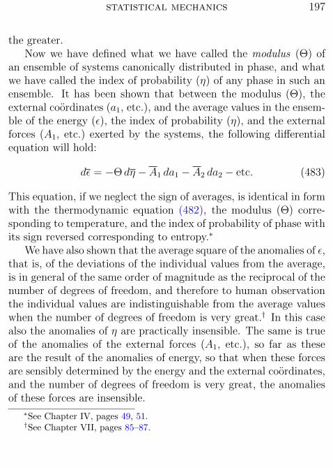
statistical mechanics 197
the greater.Now we have defined what we have called the modulus (Θ) of
an ensemble of systems canonically distributed in phase, and whatwe have called the index of probability (η) of any phase in such anensemble. It has been shown that between the modulus (Θ), theexternal coordinates (a1, etc.), and the average values in the ensem-ble of the energy (ε), the index of probability (η), and the externalforces (A1, etc.) exerted by the systems, the following differentialequation will hold:
dε = −Θ dη − A1 da1 − A2 da2 − etc. (483)
This equation, if we neglect the sign of averages, is identical in formwith the thermodynamic equation (482), the modulus (Θ) corre-sponding to temperature, and the index of probability of phase withits sign reversed corresponding to entropy.∗
We have also shown that the average square of the anomalies of ε,that is, of the deviations of the individual values from the average,is in general of the same order of magnitude as the reciprocal of thenumber of degrees of freedom, and therefore to human observationthe individual values are indistinguishable from the average valueswhen the number of degrees of freedom is very great.† In this casealso the anomalies of η are practically insensible. The same is trueof the anomalies of the external forces (A1, etc.), so far as theseare the result of the anomalies of energy, so that when these forcesare sensibly determined by the energy and the external coordinates,and the number of degrees of freedom is very great, the anomaliesof these forces are insensible.
∗See Chapter IV, pages 49, 51.†See Chapter VII, pages 85–87.

statistical mechanics 198
The mathematical operations by which the finite equation be-tween ε, η, and a1, etc., is deduced from that which gives theenergy (ε) of a system in terms of the momenta (p1, . . . pn) andcoordinates both internal (q1, . . . qn) and external (a1, etc.), areindicated by the equation
e−ψΘ =
∫all· · ·
phases
∫e−
εΘ dq1 . . . dqn dp1 . . . dpn, (484)
whereψ = Θη + ε.
We have also shown that when systems of different ensemblesare brought into conditions analogous to thermal contact, the aver-age result is a passage of energy from the ensemble of the greatermodulus to that of the less,∗ or in case of equal moduli, that we havea condition of statistical equilibrium in regard to the distributionof energy.†
Propositions have also been demonstrated analogous to those inthermodynamics relating to a Carnot’s cycle,‡ or to the tendency ofentropy to increase,§ especially when bodies of different temperatureare brought into contact.¶
We have thus precisely defined quantities, and rigorously demon-strated propositions, which hold for any number of degrees of free-dom, and which, when the number of degrees of freedom (n) isenormously great, would appear to human faculties as the quanti-ties and propositions of empirical thermodynamics.
∗See Chapter XIII, page 187.†See Chapter IV, pages 39–41.‡See Chapter XIII, pages 189, 191.§See Chapter XII, pages 168–177.¶See Chapter XIII, page 186.

statistical mechanics 199
It is evident, however, that there may be more than one quantitydefined for finite values of n, which approach the same limit, whenn is increased indefinitely, and more than one proposition relating tofinite values of n, which approach the same limiting form for n =∞.There may be therefore, and there are, other quantities which maybe thought to have some claim to be regarded as temperature andentropy with respect to systems of a finite number of degrees offreedom.
The definitions and propositions which we have been consideringrelate essentially to what we have called a canonical ensemble ofsystems. This may appear a less natural and simple conceptionthan what we have called a microcanonical ensemble of systems, inwhich all have the same energy, and which in many cases representssimply the time-ensemble, or ensemble of phases through which asingle system passes in the course of time.
It may therefore seem desirable to find definitions and proposi-tions relating to these microcanonical ensembles, which shall corre-spond to what in thermodynamics are based on experience. Nowthe differential equation
dε = e−φV d log V − A1 |ε da1 − A2 |ε da2 − etc., (485)
which has been demonstrated in Chapter X, and which relates toa microcanonical ensemble, A1 |ε denoting the average value of A1
in such an ensemble, corresponds precisely to the thermodynamicequation, except for the sign of average applied to the externalforces. But as these forces are not entirely determined by the energywith the external coordinates, the use of average values is entirelygermane to the subject, and affords the readiest means of gettingperfectly determined quantities. These averages, which are takenfor a microcanonical ensemble, may seem from some points of view

statistical mechanics 200
a more simple and natural conception than those which relate toa canonical ensemble. Moreover, the energy, and the quantity cor-responding to entropy, are free from the sign of average in thisequation.
The quantity in the equation which corresponds to entropyis log V , the quantity V being defined as the extension-in-phasewithin which the energy is less than a certain limiting value (ε).This is certainly a more simple conception than the average value ina canonical ensemble of the index of probability of phase. Log V hasthe property that when it is constant
dε = −A1 |ε da1 − A2 |ε da2 + etc., (486)
which closely corresponds to the thermodynamic property of en-tropy, that when it is constant
dε = −A1 da1 − A2 da2 + etc. (487)
The quantity in the equation which corresponds to temperature ise−φV , or dε/d log V . In a canonical ensemble, the average value ofthis quantity is equal to the modulus, as has been shown by differentmethods in Chapters IX and X.
In Chapter X it has also been shown that if the systems ofa microcanonical ensemble consist of parts with separate energies,the average value of e−φV or any part is equal to its average valuefor any other part, and to the uniform value of the same expressionfor the whole ensemble. This corresponds to the theorem in thetheory of heat that in case of thermal equilibrium the temperaturesof the parts of a body are equal to one another and to that of thewhole body. Since the energies of the parts of a body cannot besupposed to remain absolutely constant, even where this is the casewith respect to the whole body, it is evident that if we regard the

statistical mechanics 201
temperature as a function of the energy, the taking of average orof probable values, or some other statistical process, must be usedwith reference to the parts, in order to get a perfectly definite valuecorresponding to the notion of temperature.
It is worthy of notice in this connection that the average valueof the kinetic energy, either in a microcanonical ensemble, or in acanonical, divided by one half the number of degrees of freedom, isequal to e−φV , or to its average value, and that this is true not onlyof the whole system which is distributed either microcanonicallyor canonically, but also of any part, although the correspondingtheorem relating to temperature hardly belongs to empirical ther-modynamics, since neither the (inner) kinetic energy of a body, norits number of degrees of freedom is immediately cognizable to ourfaculties, and we meet the gravest difficulties when we endeavor toapply the theorem to the theory of gases, except in the simplestcase, that of the gases known as monatomic.
But the correspondence between e−φV or dε/d log V and tem-perature is imperfect. If two isolated systems have such energiesthat
dε1d log V1
=dε2
d log V2
,
and the two systems are regarded as combined to form a third sys-tem with energy
ε12 = ε1 + ε2,
we shall not have in general
dε12
d log V12
=dε1
d log V1
=dε2
d log V2
,
as analogy with temperature would require. In fact, we have seen

statistical mechanics 202
thatdε12
d log V12
=dε1
d log V1
∣∣∣∣ε12
=dε2
d log V2
∣∣∣∣ε12
,
where the second and third members of the equation denote averagevalues in an ensemble in which the compound system is microcanon-ically distributed in phase. Let us suppose the two original systemsto be identical in nature. Then
ε1 = ε2 = ε1 |ε12= ε2 |ε12
.
The equation in question would require that
dε1d log V1
=dε1
d log V1
∣∣∣∣ε12
,
i.e., that we get the same result, whether we take the value ofdε1/d log V1 determined for the average value of ε1 in the ensemble,or take the average value of dε1/d log V1. This will be the casewhere dε1/d log V1 is a linear function of ε1. Evidently this doesnot constitute the most general case. Therefore the equation inquestion cannot be true in general. It is true, however, in somevery important particular cases, as when the energy is a quadraticfunction of the p’s and q’s, or of the p’s alone.∗ When the equationholds, the case is analogous to that of bodies in thermodynamicsfor which the specific heat for constant volume is constant.
Another quantity which is closely related to temperature isdφ/dε. It has been shown in Chapter IX that in a canonical en-semble, if n > 2, the average value of dφ/dε is 1/Θ, and that the
∗This last case is important on account of its relation to the theory of gases,although it must in strictness be regarded as a limit of possible cases, ratherthan as a case which is itself possible.

statistical mechanics 203
most common value of the energy in the ensemble is that for whichdφ/dε = 1/Θ. The first of these properties may be compared withthat of dε/d log V , which has been seen to have the average value Θin a canonical ensemble, without restriction in regard to the numberof degrees of freedom.
With respect to microcanonical ensembles also, dφ/dε has aproperty similar to what has been mentioned with respect todε/d log V . That is, if a system microcanonically distributed inphase consists of two parts with separate energies, and each withmore than two degrees of freedom, the average values in the ensem-ble of dφ/dε for the two parts are equal to one another and to thevalue of same expression for the whole. In our usual notations
dφ1
dε1
∣∣∣∣ε12
=dφ2
dε2
∣∣∣∣ε12
=dφ12
dε12
if n1 > 2, and n2 > 2.This analogy with temperature has the same incompleteness
which was noticed with respect to dε/d log V , viz., if two systemshave such energies (ε1 and ε2) that
dφ1
dε1=dφ2
dε2,
and they are combined to form a third system with energy
ε12 = ε1 + ε2,
we shall not have in general
dφ12
dε12
=dφ1
dε1=dφ2
dε2.

statistical mechanics 204
Thus, if the energy is a quadratic function of the p’s and q’s, wehave∗
dφ1
dε1=n1 − 1
ε1,
dφ2
dε2=n2 − 1
ε2,
dφ12
dε12
=n12 − 1
ε12
=n1 + n2 − 1
ε1 + ε2,
where n1, n2, n12, are the numbers of degrees of freedom of theseparate and combined systems. But
dφ1
dε1=dφ2
dε2=n1 + n2 − 2
ε1 + ε2.
If the energy is a quadratic function of the p’s alone, the case wouldbe the same except that we should have 1
2n1, 1
2n2, 1
2n12, instead of
n1, n2, n12. In these particular cases, the analogy between dε/d log Vand temperature would be complete, as has already been remarked.We should have
dε1d log V1
=ε1n1
,dε2
d log V2
=ε2n2
,
dε12
d log V12
=ε12
n12
=dε1
d log V1
=dε2
d log V2
,
when the energy is a quadratic function of the p’s and q’s, andsimilar equations with 1
2n1, 1
2n2, 1
2n12, instead of n1, n2, n12, when
the energy is a quadratic function of the p’s alone.More characteristic of dφ/dε are its properties relating to most
probable values of energy. If a system having two parts with sep-arate energies and each with more than two degrees of freedom is
∗See foot-note on page 109. We have here made the least value of the energyconsistent with the values of the external coordinates zero instead of εα, as isevidently allowable when the external coordinates are supposed invariable.

statistical mechanics 205
microcanonically distributed in phase, the most probable divisionof energy between the parts, in a system taken at random from theensemble, satisfies the equation
dφ1
dε1=dφ2
dε2, (488)
which corresponds to the thermodynamic theorem that the distri-bution of energy between the parts of a system, in case of thermalequilibrium, is such that the temperatures of the parts are equal.
To prove the theorem, we observe that the fractional part of thewhole number of systems which have the energy of one part (ε1)between the limits ε′1 and ε′′1 is expressed by
e−φ12
∫ ε′′1
ε′1
eφ1+φ2 dε1,
where the variables are connected by the equation
ε1 + ε2 = constant = e12.
The greatest value of this expression, for a constant infinitesimalvalue of the difference ε′′1 − ε′1, determines a value of ε1, which wemay call its most probable value. This depends on the greatestpossible value of φ1 + φ2. Now if n1 > 2, and n2 > 2, we shallhave φ1 = −∞ for the least possible value of ε1, and φ2 = −∞for the least possible value of ε2. Between these limits φ1 and φ2
will be finite and continuous. Hence φ1 + φ2 will have a maximumsatisfying the equation (488).
But if n1 ≤ 2, or n2 ≤ 2, dφ1/dε1 or dφ2/2ε2 may be negative, orzero, for all values of ε1 or ε2, and can hardly be regarded as havingproperties analogous to temperature.

statistical mechanics 206
It is also worthy of notice that if a system which is microcanon-ically distributed in phase has three parts with separate energies,and each with more than two degrees of freedom, the most probabledivision of energy between these parts satisfies the equation
dφ1
dε1=dφ2
dε2=dφ3
dε3.
That is, this equation gives the most probable set of values of ε1, ε2,and ε3. But it does not give the most probable value of ε1, or of ε2, orof ε3. Thus, if the energies are quadratic functions of the p’s and q’s,the most probable division of energy is given by the equation
n1 − 1
ε1=n2 − 1
ε2=n3 − 1
ε3.
But the most probable value of ε1 is given by
n1 − 1
ε1=n2 + n3 − 1
ε2 + ε3,
while the preceding equations give
n1 − 1
ε1=n2 + n3 − 2
ε2 + ε3.
These distinctions vanish for very great values of n1, n2, n3. Forsmall values of these numbers, they are important. Such facts seemto indicate that the consideration of the most probable division ofenergy among the parts of a system does not afford a convenientfoundation for the study of thermodynamic analogies in the case ofsystems of a small number of degrees of freedom. The fact that acertain division of energy is the most probable has really no especialphysical importance, except when the ensemble of possible divisions

statistical mechanics 207
are grouped so closely together that the most probable division mayfairly represent the whole. This is in general the case, to a very closeapproximation, when n is enormously great; it entirely fails whenn is small.
If we regard dφ/dε as corresponding to the reciprocal of temper-ature, or, in other words, dε/dφ as corresponding to temperature,φ will correspond to entropy. It has been defined as log(dV/dε). Inthe considerations on which its definition is founded, it is thereforevery similar to log V . We have seen that dφ/d log V approaches thevalue unity when n is very great.∗
To form a differential equation on the model of the thermody-namic equation (482), in which dε/dφ shall take the place of tem-perature, and φ of entropy, we may write
dε =
(dε
dφ
)α
dφ+
(dε
da1
)φ,α
da1 +
(dε
da2
)φ,α
da2 + etc., (489)
or
dφ =dφ
dεdε+
dφ
da1
da1 +dφ
da2
da2 + etc. (490)
With respect to the differential coefficients in the last equation,which corresponds exactly to (482) solved with respect to dη, wehave seen that their average values in a canonical ensemble areequal to 1/Θ, and the averages of A1/Θ, A2/Θ, etc.† We have alsoseen that dε/dφ (or dφ/dε) has relations to the most probable valuesof energy in parts of a microcanonical ensemble. That (dε/da1)φ,α,etc., have properties somewhat analogous, may be shown as follows.
In a physical experiment, we measure a force by balancing itagainst another. If we should ask what force applied to increase or
∗See Chapter X, pages 141, 142.†See Chapter IX, equations (321), (327).

statistical mechanics 208
diminish a1 would balance the action of the systems, it would beone which varies with the different systems. But we may ask whatsingle force will make a given value of a1 the most probable, and weshall find that under certain conditions (dε/da1)φ,α represents thatforce.
To make the problem definite, let us consider a system con-sisting of the original system together with another having thecoordinates a1, a2, etc., and forces A′1, A′2, etc., tending to in-crease those coordinates. These are in addition to the forces A1,A2, etc., exerted by the original system, and are derived from aforce-function (−ε′q) by the equations
A′1 = −dε′qda1
, A′2 = −dε′qda2
, etc.
For the energy of the whole system we may write
E = ε+ ε′q + 12m1a
21 + 1
2m2a
22 + etc.,
and for the extension-in-phase of the whole system within any limits∫· · ·∫dp1 . . . dqn da1m1 da1 da2m2 da2 . . . ,
or ∫· · ·∫eφ dε da1m1 da1 da2m2 da2 . . . ,
or again ∫· · ·∫eφ dE da1m1 da1 da2m2 da2 . . . ,
since dε = dE, when a1, a1, a2, a2, etc., are constant. If the limitsare expressed by E and E + dE, a1 and a1 + da1, a1 and a1 + da1,etc., the integral reduces to
eφ dE da1m1 da1 da2m2 da2 . . . .

statistical mechanics 209
The values of a1, a1, a2, a2, etc., which make this expression amaximum for constant values of the energy of the whole systemand of the differentials dE, da1, da1, etc., are what may be calledthe most probable values of a1, a1, etc., in an ensemble in which thewhole system is distributed microcanonically.
To determine these values we have
deφ = 0,
whend(ε+ ε′q + 1
2m1a
21 + 1
2m2a
22 + etc.) = 0.
That is,dφ = 0,
when(dε
dφ
)α
dφ+
(dε
da1
)φ,α
da1 − A′1 da1 + etc. +m1a1 da1 + etc. = 0.
This requiresa1 = 0, a2 = 0, etc.
and (dε
da1
)φ,α
= A′1,
(dε
da2
)φ,α
= A′2, etc.
This shows that for any given values of E, a1, a2, etc.
(dε
da1
)φ,α
,(dε
da2
)φ,α
, etc., represent the forces (in the generalized sense) which
the external bodies would have to exert to make these values of a1,a2, etc., the most probable under the conditions specified. When the

statistical mechanics 210
differences of the external forces which are exerted by the differentsystems are negligible, −(dε/da1)φ,α etc., represent these forces.
It is certainly in the quantities relating to a canonical ensemble,ε, Θ, η, A1, etc., a1, etc., that we find the most complete correspon-dence with the quantities of the thermodynamic equation (482).Yet the conception itself of the canonical ensemble may seem tosome artificial, and hardly germane to a natural exposition of the
subject; and the quantities ε,dε
d log V, log V , A1 |ε, etc., a1, etc.,
or ε,dε
dφ, φ,
(dε
da1
)φ,α
, etc., a1, etc., which are closely related to
ensembles of constant energy, and to average and most probablevalues in such ensembles, and most of which are defined withoutreference to any ensemble, may appear the most natural analoguesof the thermodynamic quantities.
In regard to the naturalness of seeking analogies with the ther-modynamic behavior of bodies in canonical or microcanonical en-sembles of systems, much will depend upon how we approach thesubject, especially upon the question whether we regard energy ortemperature as an independent variable.
It is very natural to take energy for an independent variablerather than temperature, because ordinary mechanics furnishes uswith a perfectly defined conception of energy, whereas the idea ofsomething relating to a mechanical system and corresponding totemperature is a notion but vaguely defined. Now if the state ofa system is given by its energy and the external coordinates, itis incompletely defined, although its partial definition is perfectlyclear as far as it goes. The ensemble of phases microcanonicallydistributed, with the given values of the energy and the externalcoordinates, will represent the imperfectly defined system better

statistical mechanics 211
than any other ensemble or single phase. When we approach thesubject from this side, our theorems will naturally relate to averagevalues, or most probable values, in such ensembles.
In this case, the choice between the variables of (485) or of (489)will be determined partly by the relative importance which is at-tached to average and probable values. It would seem that in gen-eral average values are the most important, and that they lendthemselves better to analytical transformations. This considerationwould give the preference to the system of variables in which log Vis the analogue of entropy. Moreover, if we make φ the analogue ofentropy, we are embarrassed by the necessity of making numerousexceptions for systems of one or two degrees of freedom.
On the other hand, the definition of φ may be regarded as a lit-tle more simple than that of log V , and if our choice is determinedby the simplicity of the definitions of the analogues of entropy andtemperature, it would seem that the φ system should have the pref-erence. In our definition of these quantities, V was defined first,and eφ derived from V by differentiation. This gives the relationof the quantities in the most simple analytical form. Yet so far asthe notions are concerned, it is perhaps more natural to regard vas derived from eφ by integration. At all events, eφ may be definedindependently of V , and its definition may be regarded as moresimple as not requiring the determination of the zero from whichV is measured, which sometimes involves questions of a delicate na-ture. In fact, the quantity eφ may exist, when the definition of Vbecomes illusory for practical purposes, as the integral by which itis determined becomes infinite.
The case is entirely different, when we regard the temperatureas an independent variable, and we have to consider a system whichis described as having a certain temperature and certain values for

statistical mechanics 212
the external coordinates. Here also the state of the system is notcompletely defined, and will be better represented by an ensembleof phases than by any single phase. What is the nature of such anensemble as will best represent the imperfectly defined state?
When we wish to give a body a certain temperature, we place itin a bath of the proper temperature, and when we regard what wecall thermal equilibrium as established, we say that the body hasthe same temperature as the bath. Perhaps we place a second bodyof standard character, which we call a thermometer, in the bath,and say that the first body, the bath, and the thermometer, haveall the same temperature.
But the body under such circumstances, as well as the bath, andthe thermometer, even if they were entirely isolated from externalinfluences (which it is convenient to suppose in a theoretical discus-sion), would be continually changing in phase, and in energy as wellas in other respects, although our means of observation are not fineenough to perceive these variations.
The series of phases through which the whole system runs in thecourse of time may not be entirely determined by the energy, butmay depend on the initial phase in other respects. In such cases theensemble obtained by the microcanonical distribution of the wholesystem, which includes all possible time-ensembles combined in theproportion which seems least arbitrary, will represent better thanany one time-ensemble the effect of the bath. Indeed a single time-ensemble, when it is not also a microcanonical ensemble, is tooill-defined a notion to serve the purposes of a general discussion.We will therefore direct our attention, when we suppose the bodyplaced in a bath, to the microcanonical ensemble of phases thusobtained.
If we now suppose the quantity of the substance forming the

statistical mechanics 213
bath to be increased, the anomalies of the separate energies of thebody and of the thermometer in the microcanonical ensemble willbe increased, but not without limit. The anomalies of the energy ofthe bath, considered in comparison with its whole energy, diminishindefinitely as the quantity of the bath is increased, and becomein a sense negligible, when the quantity of the bath is sufficientlyincreased. The ensemble of phases of the body, and of the ther-mometer, approach a standard form as the quantity of the bath isindefinitely increased. This limiting form is easily shown to be whatwe have described as the canonical distribution.
Let us write ε for the energy of the whole system consisting ofthe body first mentioned, the bath, and the thermometer (if any),and let us first suppose this system to be distributed canonicallywith the modulus Θ. We have by (205)
(ε− ε)2 = Θ2 dε
dΘ,
and since
εp =n
2Θ,
dε
dΘ=n
2
dε
dεp.
If we write ∆ε for the anomaly of mean square, we have
(∆ε)2 = (ε− ε)2.
If we set
∆Θ =dΘ
dεdε,
∆Θ will represent approximately the increase of Θ which wouldproduce an increase in the average value of the energy equal to its

statistical mechanics 214
anomaly of mean square. Now these equations give
(∆Θ)2 =2Θ2
n
dεpdε,
which shows that we may diminish ∆Θ indefinitely by increasingthe quantity of the bath.
Now our canonical ensemble consists of an infinity of micro-canonical ensembles, which differ only in consequence of the differ-ent values of the energy which is constant in each. If we considerseparately the phases of the first body which occur in the canonicalensemble of the whole system, these phases will form a canonicalensemble of the same modulus. This canonical ensemble of phasesof the first body will consist of parts which belong to the differentmicrocanonical ensembles into which the canonical ensemble of thewhole system is divided.
Let us now imagine that the modulus of the principal canonicalensemble is increased by 2 ∆Θ, and its average energy by 2 ∆ε.The modulus of the canonical ensemble of the phases of the firstbody considered separately will be increased by 2 ∆Θ. We mayregard the infinity of microcanonical ensembles into which we havedivided the principal canonical ensemble as each having its energyincreased by 2 ∆ε. Let us see how the ensembles of phases of thefirst body contained in these microcanonical ensembles are affected.We may assume that they will all be affected in about the sameway, as all the differences which come into account may be treatedas small. Therefore, the canonical ensemble formed by taking themtogether will also be affected in the same way. But we know howthis is affected. It is by the increase of its modulus by 2 ∆Θ, aquantity which vanishes when the quantity of the bath is indefinitelyincreased.

statistical mechanics 215
In the case of an infinite bath, therefore, the increase of the en-ergy of one of the microcanonical ensembles by 2 ∆ε, produces avanishing effect on the distribution in energy of the phases of thefirst body which it contains. But 2 ∆ε is more than the averagedifference of energy between the microcanonical ensembles. Thedistribution in energy of these phases is therefore the same in thedifferent microcanonical ensembles, and must therefore be canoni-cal, like that of the ensemble which they form when taken together.∗
As a general theorem, the conclusion may be expressed in thewords:—If a system of a great number of degrees of freedom ismicrocanonically distributed in phase, any very small part of it maybe regarded as canonically distributed.†
It would seem, therefore, that a canonical ensemble of phases iswhat best represents, with the precision necessary for exact mathe-matical reasoning, the notion of a body with a given temperature, ifwe conceive of the temperature as the state produced by such pro-cesses as we actually use in physics to produce a given temperature.Since the anomalies of the body increase with the quantity of thebath, we can only get rid of all that is arbitrary in the ensemble ofphases which is to represent the notion of a body of a given temper-
∗In order to appreciate the above reasoning, it should be understood thatthe differences of energy which occur in the canonical ensemble of phases of thefirst body are not here regarded as vanishing quantities. To fix one’s ideas, onemay imagine that he has the fineness of perception to make these differencesseem large. The difference between the part of these phases which belong toone microcanonical ensemble of the whole system and the part which belongs toanother would still be imperceptible, when the quantity of the bath is sufficientlyincreased.
†It is assumed—and without this assumption the theorem would have nodistinct meaning—that the part of the ensemble considered may be regardedas having separate energy.

statistical mechanics 216
ature by making the bath infinite, which brings us to the canonicaldistribution.
A comparison of temperature and entropy with their analoguesin statistical mechanics would be incomplete without a considera-tion of their differences with respect to units and zeros, and thenumbers used for their numerical specification. If we apply the no-tions of statistical mechanics to such bodies as we usually considerin thermodynamics, for which the kinetic energy is of the same or-der of magnitude as the unit of energy, but the number of degrees offreedom is enormous, the values of Θ, dε/d log V , and dε/dφ will beof the same order of magnitude as 1/n, and the variable part of η,log V , and φ will be of the same order of magnitude as n.∗ If thesequantities, therefore, represent in any sense the notions of tempera-ture and entropy, they will nevertheless not be measured in units ofthe usual order of magnitude,—a fact which must be borne in mindin determining what magnitudes may be regarded as insensible tohuman observation.
Now nothing prevents our supposing energy and time in our sta-tistical formulae to be measured in such units as may be convenientfor physical purposes. But when these units have been chosen, thenumerical values of Θ, dε/d log V , dε/dφ, η, log V , φ, are entirelydetermined,† and in order to compare them with temperature andentropy, the numerical values of which depend upon an arbitraryunit, we must multiply all values of Θ, dε/d log V , dε/dφ by a con-stant (K), and divide all values of η, log V , and φ by the same
∗See equations (124), (288), (289), and (314); also page 125.†The unit of time only affects the last three quantities, and these only by
an additive constant, which disappears (with the additive constant of entropy),when differences of entropy are compared with their statistical analogues. Seepage 20.

statistical mechanics 217
constant. This constant is the same for all bodies, and dependsonly on the units of temperature and energy which we employ. Forordinary units it is of the same order of magnitude as the numbersof atoms in ordinary bodies.
We are not able to determine the numerical value of K, as itdepends on the number of molecules in the bodies with which weexperiment. To fix our ideas, however, we may seek an expressionfor this value, based upon very probable assumptions, which willshow how we would naturally proceed to its evaluation, if our powersof observation were fine enough to take cognizance of individualmolecules.
If the unit of mass of a monatomic gas contains ν atoms, and itmay be treated as a system of 3ν degrees of freedom, which seemsto be the case, we have for canonical distribution
εp = 32νΘ,
dεpdΘ
= 32ν. (491)
If we write T for temperature, and cv for the specific heat of the gasfor constant volume (or rather the limit toward which this specificheat tends, as rarefaction is indefinitely increased), we have
dεpdT
= cv,
since we may regard the energy as entirely kinetic. We may set theεp of this equation equal to the εp of the preceding, where indeedthe individual values of which the average is taken would appear tohuman observation as identical. This gives
dΘ
dT=
2cv3ν
,

statistical mechanics 218
whence1
K=
2cv3ν
. (493)
a value recognized by physicists as a constant independent of thekind of monatomic gas considered.
We may also express the value of K in a somewhat differentform, which corresponds to the indirect method by which physicistsare accustomed to determine the quantity cv. The kinetic energydue to the motions of the centers of mass of the molecules of a massof gas sufficiently expanded is easily shown to be equal to
32pv,
where p and v denote the pressure and volume. The average valueof the same energy in a canonical ensemble of such a mass of gas is
32Θν,
where ν denotes the number of molecules in the gas. Equating thesevalues, we have
pv = Θν, (494)
whence1
K=
Θ
T=pv
νT. (495)
Now the laws of Boyle, Charles, and Avogadro may be expressedby the equation
pv = AνT, (496)
where A is a constant depending only on the units in which energyand temperature are measured. 1/K, therefore, might be called theconstant of the law of Boyle, Charles, and Avogadro as expressedwith reference to the true number of molecules in a gaseous body.

statistical mechanics 219
Since such numbers are unknown to us, it is more convenient toexpress the law with reference to relative values. If we denote by Mthe so-called molecular weight of a gas, that is, a number taken froma table of numbers proportional to the weights of various moleculesand atoms, but having one of the values, perhaps the atomic weightof hydrogen, arbitrarily made unity, the law of Boyle, Charles, andAvogadro may be written in the more practical form
pv = A′Tm
M, (497)
where A′ is a constant and m the weight of gas considered. It isevident that 1/K is equal to the product of the constant of the lawin this form and the (true) weight of an atom of hydrogen, or suchother atom or molecule as may be given the value unity in the tableof molecular weights.
In the following chapter we shall consider the necessary modi-fications in the theory of equilibrium, when the quantity of mattercontained in a system is to be regarded as variable, or, if the systemcontains more than one kind of matter, when the quantities of theseveral kinds of matter in the system are to be regarded as indepen-dently variable. This will give us yet another set of variables in thestatistical equation, corresponding to those of the amplified form ofthe thermodynamic equation.

XV.
SYSTEMS COMPOSED OF MOLECULES.
The nature of material bodies is such, that especial interest attachesto the dynamics of systems composed of a great number of entirelysimilar particles, or, it may be, of a great number of particles ofseveral kinds, all of each kind being entirely similar to each other.We shall therefore proceed to consider systems composed of suchparticles, whether in great numbers or otherwise, and especially toconsider the statistical equilibrium of ensembles of such systems.One of the variations to be considered in regard to such systems isa variation in the numbers of the particles of the various kinds whichit contains, and the question of statistical equilibrium between twoensembles of such systems relates in part to the tendencies of thevarious kinds of particles to pass from the one to the other.
First of all, we must define precisely what is meant by statis-tical equilibrium of such an ensemble of systems. The essence ofstatistical equilibrium is the permanence of the number of systemswhich fall within any given limits with respect to phase. We havetherefore to define how the term “phase” is to be understood insuch cases. If two phases differ only in that certain entirely simi-lar particles have changed places with one another, are they to beregarded as identical or different phases? If the particles are re-garded as indistinguishable, it seems in accordance with the spiritof the statistical method to regard the phases as identical. In fact,it might be urged that in such an ensemble of systems as we areconsidering no identity is possible between the particles of differentsystems except that of qualities, and if ν particles of one systemare described as entirely similar to one another and to ν of anothersystem, nothing remains on which to base the identification of any

statistical mechanics 221
particular particle of the first system with any particular particleof the second. And this would be true, if the ensemble of systemshad a simultaneous objective existence. But it hardly applies tothe creations of the imagination. In the cases which we have beenconsidering, and in those which we shall consider, it is not onlypossible to conceive of the motion of an ensemble of similar systemssimply as possible cases of the motion of a single system, but it isactually in large measure for the sake of representing more clearlythe possible cases of the motion of a single system that we use theconception of an ensemble of systems. The perfect similarity ofseveral particles of a system will not in the least interfere with theidentification of a particular particle in one case with a particularparticle in another. The question is one to be decided in accordancewith the requirements of practical convenience in the discussion ofthe problems with which we are engaged.
Our present purpose will often require us to use the terms phase,density-in-phase, statistical equilibrium, and other connected termson the supposition that phases are not altered by the exchange ofplaces between similar particles. Some of the most important ques-tions with which we are concerned have reference to phases thusdefined. We shall call them phases determined by generic defini-tions, or briefly, generic phases. But we shall also be obliged todiscuss phases defined by the narrower definition (so that exchangeof position between similar particles is regarded as changing thephase), which will be called phases determined by specific defini-tions, or briefly, specific phases. For the analytical description of aspecific phase is more simple than that of a generic phase. And itis a more simple matter to make a multiple integral extend over allpossible specific phases than to make one extend without repetitionover all possible generic phases.

statistical mechanics 222
It is evident that if ν1, ν2, . . . νh, are the numbers of the dif-ferent kinds of molecules in any system, the number of specificphases embraced in one generic phase is represented by the con-tinued product ν1! ν2! · · · νh! and the coefficient of probability of ageneric phase is the sum of the probability-coefficients of the specificphases which it represents. When these are equal among themselves,the probability-coefficient of the generic phase is equal to that ofthe specific phase multiplied by ν1! ν2! · · · νh!. It is also evident thatstatistical equilibrium may subsist with respect to generic phaseswithout statistical equilibrium with respect to specific phases, butnot vice versa.
Similar questions arise where one particle is capable of severalequivalent positions. Does the change from one of these positionsto another change the phase? It would be most natural and logi-cal to make it affect the specific phase, but not the generic. Thenumber of specific phases contained in a generic phase would thenbe ν1!κν1
1 · · · νh!κνhh , where κ1, . . .κh denote the numbers of equiva-
lent positions belonging to the several kinds of particles. The casein which a κ is infinite would then require especial attention. Itdoes not appear that the resulting complications in the formulaewould be compensated by any real advantage. The reason of thisis that in problems of real interest equivalent positions of a particlewill always be equally probable. In this respect, equivalent posi-tions of the same particle are entirely unlike the ν! different ways inwhich ν particles may be distributed in ν different positions. Let ittherefore be understood that in spite of the physical equivalence ofdifferent positions of the same particle they are to be considered asconstituting a difference of generic phase as well as of specific. Thenumber of specific phases contained in a generic phase is thereforealways given by the product ν1! ν2! · · · νh!.

statistical mechanics 223
Instead of considering, as in the preceding chapters, ensembles ofsystems differing only in phase, we shall now suppose that the sys-tems constituting an ensemble are composed of particles of variouskinds, and that they differ not only in phase but also in the num-bers of these particles which they contain. The external coordinatesof all the systems in the ensemble are supposed, as heretofore, tohave the same value, and when they vary, to vary together. Fordistinction, we may call such an ensemble a grand ensemble, andone in which the systems differ only in phase a petit ensemble. Agrand ensemble is therefore composed of a multitude of petit en-sembles. The ensembles which we have hitherto discussed are petitensembles.
Let ν1, . . . νh, etc., denote the numbers of the different kindsof particles in a system, ε its energy, and q1, . . . qn, p1, . . . pn itscoordinates and momenta. If the particles are of the nature of ma-terial points, the number of coordinates (n) of the system will beequal to 3ν1 + · · ·+ 3νh. But if the particles are less simple in theirnature, if they are to be treated as rigid solids, the orientation ofwhich must be regarded, or if they consist each of several atoms,so as to have more than three degrees of freedom, the number ofcoordinates of the system will be equal to the sum of ν1, ν2, etc.,multiplied each by the number of degrees of freedom of the kind ofparticle to which it relates.
Let us consider an ensemble in which the number of systemshaving ν1, . . . νh particles of the several kinds, and having valuesof their coordinates and momenta lying between the limits q1 andq1 + dq1, p1 and p1 + dp1, etc., is represented by the expression
NeΩ+µ1ν1+···+µhνh−ε
Θ
ν1! · · · νh!dp1 . . . dqn, (498)

statistical mechanics 224
where N , Ω, µ1, . . .µh are constants, N denoting the total numberof systems in the ensemble. The expression
NeΩ+µ1ν1+···+µhνh−ε
Θ
ν1! · · · νh!(499)
evidently represents the density-in-phase of the ensemble within thelimits described, that is, for a phase specifically defined. The ex-pression
eΩ+µ1ν1+···+µhνh−ε
Θ
ν1! · · · νh!dp1 . . . dqn, (500)
is therefore the probability-coefficient for a phase specifically de-fined. This has evidently the same value for all the ν1! · · · νh! phasesobtained by interchanging the phases of particles of the same kind.The probability-coefficient for a generic phase will be ν1! · · · νh!times as great, viz.,
eΩ+µ1ν1+···+µhνh−ε
Θ . (501)
We shall say that such an ensemble as has been described iscanonically distributed, and shall call the constant Θ its modulus.It is evidently what we have called a grand ensemble. The petitensembles of which it is composed are canonically distributed, ac-cording to the definitions of Chapter IV, since the expression
eΩ+µ1ν1+···+µhνh
Θ
ν1! · · · νh!(502)
is constant for each petit ensemble. The grand ensemble, therefore,is in statistical equilibrium with respect to specific phases.
If an ensemble, whether grand or petit, is identical so far asgeneric phases are concerned with one canonically distributed, we

statistical mechanics 225
shall say that its distribution is canonical with respect to genericphases. Such an ensemble is evidently in statistical equilibrium withrespect to generic phases, although it may not be so with respectto specific phases.
If we write H for the index of probability of a generic phase ina grand ensemble, we have for the case of canonical distribution
H =Ω + µ1ν1 + · · ·+ µhνh − ε
Θ. (503)
It will be observed that the H is a linear function of ε and ν1, . . . νh;also that whenever the index of probability of generic phases in agrand ensemble is a linear function of ε, ν1, . . . νh, the ensemble iscanonically distributed with respect to generic phases.
The constant Ω we may regard as determined by the equation
N =∑ν1
· · ·∑νh
∫all· · ·
phases
∫Ne
Ω+µ1ν1+···+µhνh−εΘ
ν1! · · · νh!dp1 . . . dqn, (504)
or
e−ΩΘ =
∑ν1
· · ·∑νh
eµ1ν1+···+µhνh
Θ
ν1! · · · νh!
∫all· · ·
phases
∫e−
εΘ dp1 . . . dqn, (505)
where the multiple sum indicated by∑
ν1· · ·∑
νhincludes all terms
obtained by giving to each of the symbols ν1, . . . νh all integralvalues from zero upward, and the multiple integral (which is to beevaluated separately for each term of the multiple sum) is to beextended over all the (specific) phases of the system having thespecified numbers of particles of the various kinds. The multiple
integral in the last equation is what we have represented by e−ψΘ .

statistical mechanics 226
See equation(92). We may therefore write
e−ΩΘ =
∑ν1
· · ·∑νh
eµ1ν1+···+µhνh−ψ
Θ
ν1! · · · νh!. (506)
It should be observed that the summation includes a term inwhich all the symbols ν1, . . . νh have the value zero. We must there-fore recognize in a certain sense a system consisting of no particles,which, although a barren subject of study in itself, cannot well beexcluded as a particular case of a system of a variable number ofparticles. In this case ε is constant, and there are no integrationsto be performed. We have therefore∗
e−ψΘ = e−
εΘ , i.e., ψ = ε.
The value of εp is of course zero in this case. But the value of εqcontains an arbitrary constant, which is generally determined byconsiderations of convenience, so that εq and ε do not necessarilyvanish with ν1, . . . νh.
Unless −Ω has a finite value, our formulae become illusory. Wehave already, in considering petit ensembles canonically distributed,found it necessary to exclude cases in which −ψ has not a finitevalue.† The same exclusion would here make −ψ finite for anyfinite values of ν1, . . . νh. This does not necessarily make a multipleseries of the form (506) finite. We may observe, however, that if forall values of ν1, . . . νh
−ψ ≤ c0 + c1ν1 + · · ·+ chνh, (507)
∗This conclusion may appear a little strained. The original definition of ψmay not be regarded as fairly applying to systems of no degrees of freedom. Wemay therefore prefer to regard these equations as defining ψ in this case.
†See Chapter IV, page 39.

statistical mechanics 227
where c0, c1, . . . ch are constants or functions of Θ,
e−ΩΘ ≤
∑ν1
· · ·∑νh
ec0+(µ1+c1)ν1+···+(µh+ch)νh
Θ
ν1! · · · νh!,
i.e.
e−ΩΘ ≤ e
c0Θ
∑ν1
eµ1+c1
Θν1
ν1!· · ·∑νh
eµh+ch
Θνh
νh!,
i.e.
e−ΩΘ ≤ e
c0Θ ee
µ1+c1Θ
ν1 · · · eeµh+ch
Θνh,
i.e.
−Ω
Θ≤ c0
Θ+ e
µ1+c1Θ
ν1 + · · ·+ eµh+ch
Θνh . (508)
The value of −Ω will therefore be finite, when the condition (507) issatisfied. If therefore we assume that −Ω is finite, we do not appearto exclude any cases which are analogous to those of nature.∗
The interest of the ensemble which has been described lies inthe fact that it may be in statistical equilibrium, both in respectto exchange of energy and exchange of particles, with other grandensembles canonically distributed and having the same values of Θ
∗If the external coordinates determine a certain volume within which thesystem is confined, the contrary of (507) would imply that we could obtain aninfinite amount of work by crowding an infinite quantity of matter into a finitevolume.

statistical mechanics 228
and of the coefficients µ1, µ2, etc., when the circumstances are suchthat exchange of energy and of particles are possible, and whenequilibrium would not subsist, were it not for equal values of theseconstants in the two ensembles.
With respect to the exchange of energy, the case is exactly thesame as that of the petit ensembles considered in Chapter IV, andneeds no especial discussion. The question of exchange of particlesis to a certain extent analogous, and may be treated in a somewhatsimilar manner. Let us suppose that we have two grand ensem-bles canonically distributed with respect to specific phases, with thesame value of the modulus and of the coefficients µ1, . . .µh, and letus consider the ensemble of all the systems obtained by combiningeach system of the first ensemble with each of the second.
The probability-coefficient of a generic phase in the first ensem-ble may be expressed by
eΩ′+µ1ν′1+···+µhν′h−ε
′
Θ . (509)
The probability-coefficient of a specific phase will then be expressedby
eΩ′+µ1ν′1+···+µhν′h−ε
′
Θ
ν ′1! · · · ν ′h!, (510)
since each generic phase comprises ν1! · · · νh! specific phases. Inthe second ensemble the probability-coefficients of the generic andspecific phases will be
eΩ′′+µ1ν′′1 +···+µhν′′h−ε
′′
Θ , (511)
and
eΩ′′+µ1ν′′1 +···+µhν′′h−ε
′′
Θ
ν ′′1 ! · · · ν ′′h!. (512)

statistical mechanics 229
The probability-coefficient of a generic phase in the third ensem-ble, which consists of systems obtained by regarding each systemof the first ensemble combined with each of the second as form-ing a system, will be the product of the probability-coefficients ofthe generic phases of the systems combined, and will therefore berepresented by the formula
eΩ′′′+µ1ν′′′1 +···+µhν′′′h −ε
′′′
Θ (513)
where Ω′′′ = Ω′ + Ω′′, ε′′′ = ε′ + ε′′, ν ′′′1 = ν ′1 + ν ′′1 , etc. It willbe observed that ν ′′′1 , etc., represent the numbers of particles ofthe various kinds in the third ensemble, and ε′′′ its energy; alsothat Ω′′′ is a constant. The third ensemble is therefore canonicallydistributed with respect to generic phases.
If all the systems in the same generic phase in the third ensemblewere equably distributed among the ν ′′′1 ! · · · ν ′′′h ! specific phases whichare comprised in the generic phase, the probability-coefficient of aspecific phase would be
eΩ′′′+µ1ν′′′1 +···+µhν′′′h −ε
′′′
Θ
ν ′′′1 ! · · · ν ′′′h !. (514)
In fact, however, the probability-coefficient of any specific phasewhich occurs in the third ensemble is
eΩ′′′+µ1ν′′′1 +···+µhν′′′h −ε
′′′
Θ
ν ′1! · · · ν ′h! ν ′′1 ! · · · ν ′′h!, (515)
which we get by multiplying the probability-coefficients of specificphases in the first and second ensembles. The difference between the

statistical mechanics 230
formulae (514) and (515) is due to the fact that the generic phasesto which (513) relates include not only the specific phases occurringin the third ensemble and having the probability-coefficient (515),but also all the specifier phases obtained from these by interchangeof similar particles between two combined systems. Of these theprobability-coefficient is evidently zero, as they do not occur in theensemble.
Now this third ensemble is in statistical equilibrium, with respectboth to specific and generic phases, since the ensembles from whichit is formed are so. This statistical equilibrium is not dependenton the equality of the modulus and the coefficients µ1, . . .µh in thefirst and second ensembles. It depends only on the fact that the twooriginal ensembles were separately in statistical equilibrium, andthat there is no interaction between them, the combining of the twoensembles to form a third being purely nominal, and involving nophysical connection. This independence of the systems, determinedphysically by forces which prevent particles from passing from onesystem to the other, or coming within range of each other’s action,is represented mathematically by infinite values of the energy forparticles in a space dividing the systems. Such a space may becalled a diaphragm.
If we now suppose that, when we combine the systems of thetwo original ensembles, the forces are so modified that the energyis no longer infinite for particles in all the space forming the di-aphragm, but is diminished in a part of this space, so that it ispossible for particles to pass from one system to the other, this willinvolve a change in the function ε′′′ which represents the energy ofthe combined systems, and the equation ε′′′ = ε′ + ε′′ will no longerhold. Now if the coefficient of probability in the third ensemble wererepresented by (513) with this new function ε′′′, we should have sta-

statistical mechanics 231
tistical equilibrium, with respect to generic phases, although not tospecific. But this need involve only a trifling change in the distri-bution of the third ensemble,∗ a change represented by the additionof comparatively few systems in which the transference of particlesis taking place to the immense number obtained by combining thetwo original ensembles. The difference between the ensemble whichwould be in statistical equilibrium, and that obtained by combiningthe two original ensembles may be diminished without limit, whileit is still possible for particles to pass from one system to another.In this sense we may say that the ensemble formed by combining thetwo given ensembles may still be regarded as in a state of (approx-imate) statistical equilibrium with respect to generic phases, whenit has been made possible for particles to pass between the sys-tems combined, and when statistical equilibrium for specific phaseshas therefore entirely ceased to exist, and when the equilibriumfor generic phases would also have entirely ceased to exist, if thegiven ensembles had not been canonically distributed, with respectto generic phases, with the same values of Θ and µ1, . . .µh.
It is evident also that considerations of this kind will apply sepa-rately to the several kinds of particles. We may diminish the energyin the space forming the diaphragm for one kind of particle and notfor another. This is the mathematical expression for a “semiper-meable” diaphragm. The condition necessary for statistical equilib-rium where the diaphragm is permeable only to particles to whichthe suffix ( )1 relates will be fulfilled when µ1 and Θ have the same
∗It will be observed that, so far as the distribution is concerned, very largeand infinite values of ε (for certain phases) amount to nearly the same thing,—one representing the total and the other the nearly total exclusion of the phasesin question. An infinite change, therefore, in the value of ε (for certain phases)may represent a vanishing change in the distribution.

statistical mechanics 232
values in the two ensembles, although the other coefficients µ2, etc.,may be different.
This important property of grand ensembles with canonical dis-tribution will supply the motive for a more particular examinationof the nature of such ensembles, and especially of the comparativenumbers of systems in the several petit ensembles which make up agrand ensemble, and of the average values in the grand ensemble ofsome of the most important quantities, and of the average squaresof the deviations from these average values.
The probability that a system taken at random from a grandensemble canonically distributed will have exactly ν1, . . . νh particlesof the various kinds is expressed by the multiple integral∫
all· · ·phases
∫e
Ω+µ1ν1+···+µhνh−εΘ
ν1! · · · νh!dp1 . . . dqn, (516)
or
eΩ+µ1ν1+···+µhνh−ψ
Θ
ν1! · · · νh!(517)
This may be called the probability of the petit ensemble (ν1, . . . νh).The sum of all such probabilities is evidently unity. That is,
∑ν1
· · ·∑νh
eΩ+µ1ν1+···+µhνh−ψ
Θ
ν1! · · · νh!= 1, (518)
which agrees with (506).The average value in the grand ensemble of any quantity u, is
given by the formula
u =∑ν1
· · ·∑νh
∫all· · ·
phases
∫u e
Ω+µ1ν1+···+µhνh−εΘ
ν1! · · · νh!dp1 . . . dqn. (519)

statistical mechanics 233
If u is a function of ν1, . . . νh alone, i.e., if it has the same value inall systems of any same petit ensemble, the formula reduces to
u =∑ν1
· · ·∑νh
u eΩ+µ1ν1+···+µhνh−ψ
Θ
ν1! · · · νh!. (520)
Again, if we write u |grand and u |petit to distinguish averages in thegrand and petit ensembles, we shall have
u |grand =∑ν1
· · ·∑νh
u |petit
eΩ+µ1ν1+···+µhνh−ψ
Θ
ν1! · · · νh!. (521)
In this chapter, in which we are treating of grand ensembles,u will always denote the average for a grand ensemble. In thepreceding chapters, u has always denoted the average for a petitensemble.
Equation (505), which we repeat in a slightly different form, viz.,
e−ΩΘ =
∑ν1
· · ·∑νh
∫all· · ·
phases
∫eµ1ν1+···+µhνh−ε
Θ
ν1! · · · νh!dp1 . . . dqn, (522)
shows that Ω is a function of Θ and µ1, . . .µh; also of the externalcoordinates a1, a2, etc., which are involved implicitly in ε. If wedifferentiate the equation regarding all these quantities as variable,

statistical mechanics 234
we have
e−ΩΘ
(−dΩ
Θ+
Ω
Θ2dΘ
)= −dΘ
Θ
∑ν1
· · ·∑νh
∫all· · ·
phases
∫(µ1ν1 + · · ·+ µhνh − ε) e
µ1ν1+···+µhνh−εΘ
ν1! · · · νh!dp1 . . . dqn
+dµ1
Θ
∑ν1
· · ·∑νh
∫all· · ·
phases
∫ν1 e
µ1ν1+···+µhνh−εΘ
ν1! · · · νh!dp1 . . . dqn
+ etc.
− da1
Θ
∑ν1
· · ·∑νh
∫all· · ·
phases
∫dε
da1
eµ1ν1+···+µhνh−ε
Θ
ν1! · · · νh!dp1 . . . dqn
− etc. (523)
If we multiply this equation by eΩΘ , and set as usual A1, A2, etc.,
for −dε/da1, −dε/da2, etc., we get in virtue of the law expressed byequation (519),
−dΩ
Θ+
Ω
Θ2= −dΘ
Θ2(µ1ν1 + · · ·µhνh − ε)
+dµ1
Θν1 +
dµ2
Θν2 + etc.
+da1
ΘA1 +
da2
ΘA2 + etc.; (524)

statistical mechanics 235
that is,
dΩ =Ω + µ1ν1 + · · ·+ µhνh − ε
ΘdΘ−
∑ν1 dµ1 −
∑A1 da1.
(525)Since equation (503) gives
Ω + µ1ν1 + · · ·+ µhνh − εΘ
= H, (526)
the preceding equation may be written
dΩ = H dΘ−∑
ν1 dµ1 −∑
A1 da1. (527)
Again, equation (526) gives
dΩ +∑
µ1 dν1 +∑
ν1 dµ1 − dε = Θ dH + H dΘ. (528)
Eliminating dΩ from these equations, we get
dε = −Θ dH +∑
µ1 dν1 −∑
A1 da1. (529)
If we set
Ψ = ε+ ΘH, (530)
dΨ = dε+ Θ dH + H dΘ, (531)
we havedΨ = H dΘ +
∑µ1 dν1 −
∑A1 da1. (532)
The corresponding thermodynamic equations are
dε = T dη +∑
µ1 dm1 −∑
A1 da1, (533)
ψ = ε− Tη, (534)
dψ = −η dT +∑
µ1 dm1 −∑
A1 da1. (535)

statistical mechanics 236
These are derived from the thermodynamic equations (114) and(117) by the addition of the terms necessary to take account ofvariation in the quantities (m1, m2, etc.) of the several substancesof which a body is composed. The correspondence of the equationsis most perfect when the component substances are measured insuch units that m1, m2, etc., are proportional to the numbers of thedifferent kinds of molecules or atoms. The quantities µ1, µ2, etc.,in these thermodynamic equations may be defined as differentialcoefficients by either of the equations in which they occur.∗
If we compare the statistical equations (529) and (532) with(114) and (112), which are given in Chapter IV, and discussed inChapter XIV, as analogues of thermodynamic equations, we findconsiderable difference. Beside the terms corresponding to the ad-ditional terms in the thermodynamic equations of this chapter, andbeside the fact that the averages are taken in a grand ensemble inone case and in a petit in the other, the analogues of entropy, Hand η, are quite different in definition and value. We shall return tothis point after we have determined the order of magnitude of theusual anomalies of ν1, . . . νh.
If we differentiate equation (518) with respect to µ1, and multi-ply by Θ, we get
∑ν1
· · ·∑νh
(dΩ
dµ1
+ ν1
)e
Ω+µ1ν1+···+µhνh−ψΘ
ν1! · · · νh!= 0, (536)
whence dΩ/dµ1 = −ν1, which agrees with (527). Differentiatingagain with respect to µ1 and to µ2, and setting
dΩ
dµ1
= −ν1,dΩ
dµ2
= −ν2,
∗Compare Transactions Connecticut Academy, Vol. III, pages 136 ff.

statistical mechanics 237
we get
∑ν1
· · ·∑νh
(d2Ω
dµ21
+(ν1 − ν1)2
Θ
)e
Ω+µ1ν1+···+µhνh−ψΘ
ν1! · · · νh!= 0, (537)
∑ν1
· · ·∑νh
(d2Ω
dµ1 dµ2
+(ν1 − ν1)(ν2 − ν2)
Θ
)e
Ω+µ1ν1+···+µhνh−ψΘ
ν1! · · · νh!= 0.
(538)
The first members of these equations represent the average valuesof the quantities in the principal parentheses. We have therefore
(ν1 − ν1)2 = ν21 − ν2
1 = −Θd2Ω
dµ21
= Θdν1
dµ1
, (539)
(ν1 − ν1)(ν2 − ν2) = ν1ν2 − ν1ν2 = −Θd2Ω
dµ1 dµ2
= Θdν1
dµ2
= Θdν2
dµ1
.
(540)
From equation (539) we may get an idea of the order of magni-tude of the divergences of ν1 from its average value in the ensemble,when that average value is great. The equation may be written
(ν1 − ν1)2
ν21
=Θ
ν21
dν1
dµ1
, (541)
The second member of this equation will in general be small whenν1 is great. Large values are not necessarily excluded, but they mustbe confined within very small limits with respect to µ. For if
(ν1 − ν1)2
ν21
>1
ν121
, (542)

statistical mechanics 238
for all values of µ1 between the limits µ′1 and µ′′1, we shall havebetween the same limits
Θ
ν321
dν1 > dµ1, (543)
and therefore
12Θ
(1
ν′ 12
1
− 1
ν′′ 1
21
)> µ′′1 − µ′1. (544)
The difference µ′′1−µ′1 is therefore numerically a very small quantity.To form an idea of the importance of such a difference, we shouldobserve that in formula (498) µ1 is multiplied by ν1 and the productsubtracted from the energy. A very small difference in the valueof µ1 may therefore be important. But since νΘ is always lessthan the kinetic energy of the system, our formula shows that µ′′1 −µ′1, even when multiplied by ν ′1 or ν ′′1, may still be regarded as aninsensible quantity.
We can now perceive the leading characteristics with respect toproperties sensible to human faculties of such an ensemble as we areconsidering (a grand ensemble canonically distributed), when theaverage numbers of particles of the various kinds are of the sameorder of magnitude as the number of molecules in the bodies whichare the subject of physical experiment. Although the ensemble con-tains systems having the widest possible variations in respect to thenumbers of the particles which they contain, these variations arepractically contained within such narrow limits as to be insensible,except for particular values of the constants of the ensemble. Thisexception corresponds precisely to the case of nature, when certainthermodynamic quantities corresponding to Θ, µ1, µ2, etc., whichin general determine the separate densities of various components

statistical mechanics 239
of a body, have certain values which make these densities indeter-minate, in other words, when the conditions are such as determinecoexistent phases of matter. Except in the case of these particularvalues, the grand ensemble would not differ to human faculties ofperception from a petit ensemble, viz., any one of the petit ensem-bles which it contains in which ν1, ν2, etc., do not sensibly differfrom their average values.
Let us now compare the quantities H and η, the average valuesof which (in a grand and a petit ensemble respectively) we have seento correspond to entropy. Since
H =Ω + µ1ν1 + · · ·+ µhνh − ε
Θ,
and
η =ψ − ε
Θ,
H− η =Ω + µ1ν1 + · · ·+ µhνh − ψ
Θ. (545)
A part of this difference is due to the fact that H relates to genericphases and η to specific. If we write ηgen for the index of probabilityfor generic phases in a petit ensemble, we have
ηgen = η + log ν1! · · · νh!, (546)
H− η = H− ηgen + log ν1! · · · νh!, (547)
H− ηgen =Ω + µ1ν1 + · · ·+ µhνh − ψ
Θ− log ν1! · · · νh!. (548)
This is the logarithm of the probability of the petit ensemble
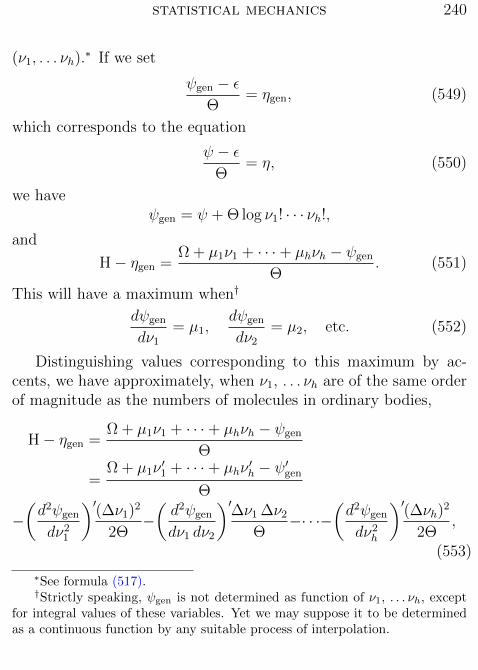
statistical mechanics 240
(ν1, . . . νh).∗ If we set
ψgen − εΘ
= ηgen, (549)
which corresponds to the equation
ψ − εΘ
= η, (550)
we haveψgen = ψ + Θ log ν1! · · · νh!,
and
H− ηgen =Ω + µ1ν1 + · · ·+ µhνh − ψgen
Θ. (551)
This will have a maximum when†
dψgen
dν1
= µ1,dψgen
dν2
= µ2, etc. (552)
Distinguishing values corresponding to this maximum by ac-cents, we have approximately, when ν1, . . . νh are of the same orderof magnitude as the numbers of molecules in ordinary bodies,
H− ηgen =Ω + µ1ν1 + · · ·+ µhνh − ψgen
Θ
=Ω + µ1ν
′1 + · · ·+ µhν
′h − ψ′gen
Θ
−(d2ψgen
dν21
)′(∆ν1)2
2Θ−(d2ψgen
dν1 dν2
)′∆ν1 ∆ν2
Θ−· · ·−
(d2ψgen
dν2h
)′(∆νh)
2
2Θ,
(553)
∗See formula (517).†Strictly speaking, ψgen is not determined as function of ν1, . . . νh, except
for integral values of these variables. Yet we may suppose it to be determinedas a continuous function by any suitable process of interpolation.

statistical mechanics 241
eH−ηgen = eCe−(d2ψgen
dν21
)′(∆ν1)2
2Θ−(d2ψgen
dν1 dν2
)′∆ν1 ∆ν2
Θ−···−
(d2ψgen
dν2h
)′(∆νh)2
2Θ ,(554)
where
C =Ω + µ1ν
′1 + · · ·+ µhν
′h − ψ′gen
Θ, (555)
and∆ν1 = ν1 − ν ′1, ∆ν2 = ν2 − ν ′2, etc. (556)
This is the probability of the system (ν1, . . . νh). The probabilitythat the values of ν1, . . . νh lie within given limits is given by themultiple integral
∫· · ·∫eCe
−(d2ψgen
dν21
)′(∆ν1)2
2Θ −(d2ψgen
dν1 dν2
)′∆ν1 ∆ν2
Θ ···−(d2ψgen
dν2h
)′(∆νh)2
2Θdν1 . . . dνh.
(557)
This shows that the distribution of the grand ensemble withrespect to the values of ν1, . . . νh follows the “law of errors” whenν ′1, . . . ν ′h are very great. The value of this integral for the limits ±∞should be unity. This gives
eC(2πΘ)
h2
D12
= 1, (558)
or
C = 12
logD − h
2log(2πΘ), (559)

statistical mechanics 242
where
D =
∣∣∣∣∣∣∣∣∣∣∣∣∣∣
(d2ψgen
dν21
)′ (d2ψgen
dν1 dν2
)′· · ·
(d2ψgen
dν1 dνh
)′(d2ψgen
dν2 dν1
)′ (d2ψgen
dν22
)′· · ·
(d2ψgen
dν2 dνh
)′· · · · · · · · · · · ·(
d2ψgen
dνh dν1
)′ (d2ψgen
dνh dν2
)′· · ·
(d2ψgen
dν2h
)′
∣∣∣∣∣∣∣∣∣∣∣∣∣∣; (560)
that is,
D =
∣∣∣∣∣∣∣∣∣∣∣∣∣∣
(dµ1
dν1
)′ (dµ1
dν2
)′· · ·
(dµ1
dνh
)′(dµ2
dν1
)′ (dµ2
dν2
)′· · ·
(dµ2
dνh
)′· · · · · · · · · · · ·(dµhdν1
)′ (dµhdν2
)′· · ·
(dµhdνh
)′
∣∣∣∣∣∣∣∣∣∣∣∣∣∣. (561)
Now, by (553), we have for the first approximation
H− ηgen = C − 12
logD − h
2log(2πΘ), (562)
and if we divide by the constant K,∗ to reduce these quantities tothe usual unit of entropy,
H− ηgen
K=
logD − h log(2πΘ)
2K. (563)
This is evidently a negligible quantity, since K is of the same orderof magnitude as the number of molecules in ordinary bodies. It is
∗See pages 216–219.

statistical mechanics 243
to be observed that ηgen is here the average in the grand ensem-
ble, whereas the quantity which we wish to compare with H is theaverage in a petit ensemble. But as we have seen that in the caseconsidered the grand ensemble would appear to human observationas a petit ensemble, this distinction may be neglected.
The differences therefore, in the case considered, between thequantities which may be represented by the notations∗
Hgen |grand , ηgen |grand , ηgen |petit
are not sensible to human faculties. The difference
ηgen |petit − ηspec |petit = ν1! · · · νh!,
and is therefore constant, so long as the numbers ν1, . . . νh are con-stant. For constant values of these numbers, therefore, it is immate-rial whether we use the average of ηgen or of η for entropy, since thisonly affects the arbitrary constant of integration which is added toentropy. But when the numbers ν1, . . . νh are varied, it is no longerpossible to use the index for specific phases. For the principle thatthe entropy of any body has an arbitrary additive constant is sub-ject to limitation, when different quantities of the same substanceare concerned. In this case, the constant being determined for onequantity of a substance, is thereby determined for all quantities ofthe same substance.
To fix our ideas, let us suppose that we have two identical fluidmasses in contiguous chambers. The entropy of the whole is equalto the sum of the entropies of the parts, and double that of one
∗In this paragraph, for greater distinctness, Hgen |grand and ηspec |petit have
been written for the quantities which elsewhere are denoted by H and η.

statistical mechanics 244
part. Suppose a valve is now opened, making a communication be-tween the chambers. We do not regard this as making any changein the entropy, although the masses of gas or liquid diffuse into oneanother, and although the same process of diffusion would increasethe entropy, if the masses of fluid were different. It is evident, there-fore, that it is equilibrium with respect to generic phases, and notwith respect to specific, with which we have to do in the evaluationof entropy, and therefore, that we must use the average of H orof ηgen, and not that of η, as the equivalent of entropy, except inthe thermodynamics of bodies in which the number of molecules ofthe various kinds is constant.

End of the Project Gutenberg EBook of Elementary Principles of Statistical
Mechanics, by Josiah Willard Gibbs
*** END OF THIS PROJECT GUTENBERG EBOOK ELEMENTARY PRINCIPLES STATISTICAL MECHANICS ***
***** This file should be named 50992-t.tex or 50992-t.zip *****
This and all associated files of various formats will be found in:
http://www.gutenberg.org/5/0/9/9/50992/
Produced by Andrew D. Hwang
Updated editions will replace the previous one--the old editions will
be renamed.
Creating the works from print editions not protected by U.S. copyright
law means that no one owns a United States copyright in these works,
so the Foundation (and you!) can copy and distribute it in the United
States without permission and without paying copyright
royalties. Special rules, set forth in the General Terms of Use part
of this license, apply to copying and distributing Project
Gutenberg-tm electronic works to protect the PROJECT GUTENBERG-tm
concept and trademark. Project Gutenberg is a registered trademark,
and may not be used if you charge for the eBooks, unless you receive
specific permission. If you do not charge anything for copies of this
eBook, complying with the rules is very easy. You may use this eBook
for nearly any purpose such as creation of derivative works, reports,
performances and research. They may be modified and printed and given
away--you may do practically ANYTHING in the United States with eBooks
not protected by U.S. copyright law. Redistribution is subject to the
trademark license, especially commercial redistribution.
START: FULL LICENSE
THE FULL PROJECT GUTENBERG LICENSE
PLEASE READ THIS BEFORE YOU DISTRIBUTE OR USE THIS WORK
To protect the Project Gutenberg-tm mission of promoting the free
distribution of electronic works, by using or distributing this work
(or any other work associated in any way with the phrase "Project
Gutenberg"), you agree to comply with all the terms of the Full
Project Gutenberg-tm License available with this file or online at
www.gutenberg.org/license.
Section 1. General Terms of Use and Redistributing Project
Gutenberg-tm electronic works

license. II
1.A. By reading or using any part of this Project Gutenberg-tm
electronic work, you indicate that you have read, understand, agree to
and accept all the terms of this license and intellectual property
(trademark/copyright) agreement. If you do not agree to abide by all
the terms of this agreement, you must cease using and return or
destroy all copies of Project Gutenberg-tm electronic works in your
possession. If you paid a fee for obtaining a copy of or access to a
Project Gutenberg-tm electronic work and you do not agree to be bound
by the terms of this agreement, you may obtain a refund from the
person or entity to whom you paid the fee as set forth in paragraph
1.E.8.
1.B. "Project Gutenberg" is a registered trademark. It may only be
used on or associated in any way with an electronic work by people who
agree to be bound by the terms of this agreement. There are a few
things that you can do with most Project Gutenberg-tm electronic works
even without complying with the full terms of this agreement. See
paragraph 1.C below. There are a lot of things you can do with Project
Gutenberg-tm electronic works if you follow the terms of this
agreement and help preserve free future access to Project Gutenberg-tm
electronic works. See paragraph 1.E below.
1.C. The Project Gutenberg Literary Archive Foundation ("the
Foundation" or PGLAF), owns a compilation copyright in the collection
of Project Gutenberg-tm electronic works. Nearly all the individual
works in the collection are in the public domain in the United
States. If an individual work is unprotected by copyright law in the
United States and you are located in the United States, we do not
claim a right to prevent you from copying, distributing, performing,
displaying or creating derivative works based on the work as long as
all references to Project Gutenberg are removed. Of course, we hope
that you will support the Project Gutenberg-tm mission of promoting
free access to electronic works by freely sharing Project Gutenberg-tm
works in compliance with the terms of this agreement for keeping the
Project Gutenberg-tm name associated with the work. You can easily
comply with the terms of this agreement by keeping this work in the
same format with its attached full Project Gutenberg-tm License when
you share it without charge with others.
1.D. The copyright laws of the place where you are located also govern
what you can do with this work. Copyright laws in most countries are
in a constant state of change. If you are outside the United States,
check the laws of your country in addition to the terms of this

license. III
agreement before downloading, copying, displaying, performing,
distributing or creating derivative works based on this work or any
other Project Gutenberg-tm work. The Foundation makes no
representations concerning the copyright status of any work in any
country outside the United States.
1.E. Unless you have removed all references to Project Gutenberg:
1.E.1. The following sentence, with active links to, or other
immediate access to, the full Project Gutenberg-tm License must appear
prominently whenever any copy of a Project Gutenberg-tm work (any work
on which the phrase "Project Gutenberg" appears, or with which the
phrase "Project Gutenberg" is associated) is accessed, displayed,
performed, viewed, copied or distributed:
This eBook is for the use of anyone anywhere in the United States and
most other parts of the world at no cost and with almost no
restrictions whatsoever. You may copy it, give it away or re-use it
under the terms of the Project Gutenberg License included with this
eBook or online at www.gutenberg.org. If you are not located in the
United States, you’ll have to check the laws of the country where you
are located before using this ebook.
1.E.2. If an individual Project Gutenberg-tm electronic work is
derived from texts not protected by U.S. copyright law (does not
contain a notice indicating that it is posted with permission of the
copyright holder), the work can be copied and distributed to anyone in
the United States without paying any fees or charges. If you are
redistributing or providing access to a work with the phrase "Project
Gutenberg" associated with or appearing on the work, you must comply
either with the requirements of paragraphs 1.E.1 through 1.E.7 or
obtain permission for the use of the work and the Project Gutenberg-tm
trademark as set forth in paragraphs 1.E.8 or 1.E.9.
1.E.3. If an individual Project Gutenberg-tm electronic work is posted
with the permission of the copyright holder, your use and distribution
must comply with both paragraphs 1.E.1 through 1.E.7 and any
additional terms imposed by the copyright holder. Additional terms
will be linked to the Project Gutenberg-tm License for all works
posted with the permission of the copyright holder found at the
beginning of this work.
1.E.4. Do not unlink or detach or remove the full Project Gutenberg-tm
License terms from this work, or any files containing a part of this

license. IV
work or any other work associated with Project Gutenberg-tm.
1.E.5. Do not copy, display, perform, distribute or redistribute this
electronic work, or any part of this electronic work, without
prominently displaying the sentence set forth in paragraph 1.E.1 with
active links or immediate access to the full terms of the Project
Gutenberg-tm License.
1.E.6. You may convert to and distribute this work in any binary,
compressed, marked up, nonproprietary or proprietary form, including
any word processing or hypertext form. However, if you provide access
to or distribute copies of a Project Gutenberg-tm work in a format
other than "Plain Vanilla ASCII" or other format used in the official
version posted on the official Project Gutenberg-tm web site
(www.gutenberg.org), you must, at no additional cost, fee or expense
to the user, provide a copy, a means of exporting a copy, or a means
of obtaining a copy upon request, of the work in its original "Plain
Vanilla ASCII" or other form. Any alternate format must include the
full Project Gutenberg-tm License as specified in paragraph 1.E.1.
1.E.7. Do not charge a fee for access to, viewing, displaying,
performing, copying or distributing any Project Gutenberg-tm works
unless you comply with paragraph 1.E.8 or 1.E.9.
1.E.8. You may charge a reasonable fee for copies of or providing
access to or distributing Project Gutenberg-tm electronic works
provided that
* You pay a royalty fee of 20% of the gross profits you derive from
the use of Project Gutenberg-tm works calculated using the method
you already use to calculate your applicable taxes. The fee is owed
to the owner of the Project Gutenberg-tm trademark, but he has
agreed to donate royalties under this paragraph to the Project
Gutenberg Literary Archive Foundation. Royalty payments must be paid
within 60 days following each date on which you prepare (or are
legally required to prepare) your periodic tax returns. Royalty
payments should be clearly marked as such and sent to the Project
Gutenberg Literary Archive Foundation at the address specified in
Section 4, "Information about donations to the Project Gutenberg
Literary Archive Foundation."
* You provide a full refund of any money paid by a user who notifies
you in writing (or by e-mail) within 30 days of receipt that s/he
does not agree to the terms of the full Project Gutenberg-tm

license. V
License. You must require such a user to return or destroy all
copies of the works possessed in a physical medium and discontinue
all use of and all access to other copies of Project Gutenberg-tm
works.
* You provide, in accordance with paragraph 1.F.3, a full refund of
any money paid for a work or a replacement copy, if a defect in the
electronic work is discovered and reported to you within 90 days of
receipt of the work.
* You comply with all other terms of this agreement for free
distribution of Project Gutenberg-tm works.
1.E.9. If you wish to charge a fee or distribute a Project
Gutenberg-tm electronic work or group of works on different terms than
are set forth in this agreement, you must obtain permission in writing
from both the Project Gutenberg Literary Archive Foundation and The
Project Gutenberg Trademark LLC, the owner of the Project Gutenberg-tm
trademark. Contact the Foundation as set forth in Section 3 below.
1.F.
1.F.1. Project Gutenberg volunteers and employees expend considerable
effort to identify, do copyright research on, transcribe and proofread
works not protected by U.S. copyright law in creating the Project
Gutenberg-tm collection. Despite these efforts, Project Gutenberg-tm
electronic works, and the medium on which they may be stored, may
contain "Defects," such as, but not limited to, incomplete, inaccurate
or corrupt data, transcription errors, a copyright or other
intellectual property infringement, a defective or damaged disk or
other medium, a computer virus, or computer codes that damage or
cannot be read by your equipment.
1.F.2. LIMITED WARRANTY, DISCLAIMER OF DAMAGES - Except for the "Right
of Replacement or Refund" described in paragraph 1.F.3, the Project
Gutenberg Literary Archive Foundation, the owner of the Project
Gutenberg-tm trademark, and any other party distributing a Project
Gutenberg-tm electronic work under this agreement, disclaim all
liability to you for damages, costs and expenses, including legal
fees. YOU AGREE THAT YOU HAVE NO REMEDIES FOR NEGLIGENCE, STRICT
LIABILITY, BREACH OF WARRANTY OR BREACH OF CONTRACT EXCEPT THOSE
PROVIDED IN PARAGRAPH 1.F.3. YOU AGREE THAT THE FOUNDATION, THE
TRADEMARK OWNER, AND ANY DISTRIBUTOR UNDER THIS AGREEMENT WILL NOT BE
LIABLE TO YOU FOR ACTUAL, DIRECT, INDIRECT, CONSEQUENTIAL, PUNITIVE OR

license. VI
INCIDENTAL DAMAGES EVEN IF YOU GIVE NOTICE OF THE POSSIBILITY OF SUCH
DAMAGE.
1.F.3. LIMITED RIGHT OF REPLACEMENT OR REFUND - If you discover a
defect in this electronic work within 90 days of receiving it, you can
receive a refund of the money (if any) you paid for it by sending a
written explanation to the person you received the work from. If you
received the work on a physical medium, you must return the medium
with your written explanation. The person or entity that provided you
with the defective work may elect to provide a replacement copy in
lieu of a refund. If you received the work electronically, the person
or entity providing it to you may choose to give you a second
opportunity to receive the work electronically in lieu of a refund. If
the second copy is also defective, you may demand a refund in writing
without further opportunities to fix the problem.
1.F.4. Except for the limited right of replacement or refund set forth
in paragraph 1.F.3, this work is provided to you ’AS-IS’, WITH NO
OTHER WARRANTIES OF ANY KIND, EXPRESS OR IMPLIED, INCLUDING BUT NOT
LIMITED TO WARRANTIES OF MERCHANTABILITY OR FITNESS FOR ANY PURPOSE.
1.F.5. Some states do not allow disclaimers of certain implied
warranties or the exclusion or limitation of certain types of
damages. If any disclaimer or limitation set forth in this agreement
violates the law of the state applicable to this agreement, the
agreement shall be interpreted to make the maximum disclaimer or
limitation permitted by the applicable state law. The invalidity or
unenforceability of any provision of this agreement shall not void the
remaining provisions.
1.F.6. INDEMNITY - You agree to indemnify and hold the Foundation, the
trademark owner, any agent or employee of the Foundation, anyone
providing copies of Project Gutenberg-tm electronic works in
accordance with this agreement, and any volunteers associated with the
production, promotion and distribution of Project Gutenberg-tm
electronic works, harmless from all liability, costs and expenses,
including legal fees, that arise directly or indirectly from any of
the following which you do or cause to occur: (a) distribution of this
or any Project Gutenberg-tm work, (b) alteration, modification, or
additions or deletions to any Project Gutenberg-tm work, and (c) any
Defect you cause.
Section 2. Information about the Mission of Project Gutenberg-tm

license. VII
Project Gutenberg-tm is synonymous with the free distribution of
electronic works in formats readable by the widest variety of
computers including obsolete, old, middle-aged and new computers. It
exists because of the efforts of hundreds of volunteers and donations
from people in all walks of life.
Volunteers and financial support to provide volunteers with the
assistance they need are critical to reaching Project Gutenberg-tm’s
goals and ensuring that the Project Gutenberg-tm collection will
remain freely available for generations to come. In 2001, the Project
Gutenberg Literary Archive Foundation was created to provide a secure
and permanent future for Project Gutenberg-tm and future
generations. To learn more about the Project Gutenberg Literary
Archive Foundation and how your efforts and donations can help, see
Sections 3 and 4 and the Foundation information page at
www.gutenberg.org
Section 3. Information about the Project Gutenberg Literary Archive Foundation
The Project Gutenberg Literary Archive Foundation is a non profit
501(c)(3) educational corporation organized under the laws of the
state of Mississippi and granted tax exempt status by the Internal
Revenue Service. The Foundation’s EIN or federal tax identification
number is 64-6221541. Contributions to the Project Gutenberg Literary
Archive Foundation are tax deductible to the full extent permitted by
U.S. federal laws and your state’s laws.
The Foundation’s principal office is in Fairbanks, Alaska, with the
mailing address: PO Box 750175, Fairbanks, AK 99775, but its
volunteers and employees are scattered throughout numerous
locations. Its business office is located at 809 North 1500 West, Salt
Lake City, UT 84116, (801) 596-1887. Email contact links and up to
date contact information can be found at the Foundation’s web site and
official page at www.gutenberg.org/contact
For additional contact information:
Dr. Gregory B. Newby
Chief Executive and Director
Section 4. Information about Donations to the Project Gutenberg

license. VIII
Literary Archive Foundation
Project Gutenberg-tm depends upon and cannot survive without wide
spread public support and donations to carry out its mission of
increasing the number of public domain and licensed works that can be
freely distributed in machine readable form accessible by the widest
array of equipment including outdated equipment. Many small donations
($1 to $5,000) are particularly important to maintaining tax exempt
status with the IRS.
The Foundation is committed to complying with the laws regulating
charities and charitable donations in all 50 states of the United
States. Compliance requirements are not uniform and it takes a
considerable effort, much paperwork and many fees to meet and keep up
with these requirements. We do not solicit donations in locations
where we have not received written confirmation of compliance. To SEND
DONATIONS or determine the status of compliance for any particular
state visit www.gutenberg.org/donate
While we cannot and do not solicit contributions from states where we
have not met the solicitation requirements, we know of no prohibition
against accepting unsolicited donations from donors in such states who
approach us with offers to donate.
International donations are gratefully accepted, but we cannot make
any statements concerning tax treatment of donations received from
outside the United States. U.S. laws alone swamp our small staff.
Please check the Project Gutenberg Web pages for current donation
methods and addresses. Donations are accepted in a number of other
ways including checks, online payments and credit card donations. To
donate, please visit: www.gutenberg.org/donate
Section 5. General Information About Project Gutenberg-tm electronic works.
Professor Michael S. Hart was the originator of the Project
Gutenberg-tm concept of a library of electronic works that could be
freely shared with anyone. For forty years, he produced and
distributed Project Gutenberg-tm eBooks with only a loose network of
volunteer support.
Project Gutenberg-tm eBooks are often created from several printed
editions, all of which are confirmed as not protected by copyright in
the U.S. unless a copyright notice is included. Thus, we do not

license. IX
necessarily keep eBooks in compliance with any particular paper
edition.
Most people start at our Web site which has the main PG search
facility: www.gutenberg.org
This Web site includes information about Project Gutenberg-tm,
including how to make donations to the Project Gutenberg Literary
Archive Foundation, how to help produce our new eBooks, and how to
subscribe to our email newsletter to hear about new eBooks.