THE PROCESSES WITH DEPENDENT INCREMENTS AS MATHEMATICAL MODELS OF

THE INTEREST RATE PROCESSES

Gennady A. Medvedev Belarussian State University, Faculty of Applied Mathematics,

4 F. Skorina avenue, Minsk 220050, Belarus Tel- (375) 17 2265879. Fax: (375) 17 2265548

E-mail- medvedev@fpm.bsu.unibel by

Abstract

Processes of the interest rates and other financial indexes in continuous time are usually

modeled in the literature by stochastic processes with independent increments. Such processes are described by the stochastic differential equations and are the Markov processes As it follows from the theory the stationary stochastic process is the Markov process (in the wide sense) if and only if the normalized correlation fimction is exponential In other words the stochastic processes with independent increments generate the data series with the exponential correlation fLnctions At the same time the correlation functions of real data series have often non-exponential correlation Kmctions. For example such functions are typical for the US Treasury Security Yield Rate, Internal Rate of Yield on UK 2 5 % Consols, UK Dividend Yield Rate for Shares and other financial data series Therefore in order that to fit a mathematical model to some real financial data it should be used a stochastic processes with dependent increments Such processes have more flexible structure that allows obtain the necessary properties In present paper it is proposed a way for the construction of the process with dependent increments For that it is supposed that the stochastic process of the interest rate (or other financial index) has a derivative of the some order and this derivative is the process with independent increments. In other words the stochastic process of the interest rate is described by the stochastic differential equation of some order more than first It results in the more relevant mathematical models. If the coefficients of stochastic differential equations are constant then the solutions in the explicit form are derived On practice the derivatives of the interest rate processes are non-observed therefore the practical forms of solutions can not include the values of derivatives Therefore it is discussed a problem of exclusion of these values from solutions. It is shown that these solutions exist and they are determined on discrete set of time instants. The case when the first derivative of process of interest rate has independent increments is described in details. The offered approach is illustrated by the analysis of actual time series of the yield rates of the US Treasury Securities.

Keywords. financial data series, mathematical model of interest rate, stochastic processes, stochastic differential equations, correlation functions, time series.

483

Introduction

Usually the stochastic models that describe a dynamics of interest rates in continuous time are based on the stochastic differential equations of first order (Shimko,l992) These equations generate the processes with independent increments that are Markov processes. In a case when such processes are stationary and their observations are produced at discrete instants, these equations result in an autoregressive models of the first order. In turn such Markov processes have only positive correlation, and according to the known Doob theorem (Doob, 1953) their correlation function is exponential. At the same time the analysis of real interest rate time series shows that their correlation functions take not only positive values, but also and negative, and they are like not an exponential curve, and rather damping cosinusoid. The author have checked this on the following financial time series:

l UK Dividend Yield Rate for Shares, December 1918 - June 1995 (919 monthly values),

l Internal Rate of Yield on LJK 2.5 % Consols, June 1900 - June 1995 (1146 monthly values);

l US Treasury Security Yield Rate: short-term debt instruments - three- monthly (13 weeks), semi-annual and annual bills, intermediate term debt instruments - 2 -, 3 -, 5 -, 7 -, I O-year notes, long-term debt instruments - 20- and 30-year bonds; January 199 1 - January 1996 (I 250 business days);

The more detailed information about these computations is contained in Medvedev (1998). The examples of such correlation Kmctions are represented on Figure 1, Such behaviour of correlation fimctions shows that mathematical models that lead to Markov processes are not always adequate to real financial time series. This problem was already considered in the literature (Ait-Sahalia, 1997, Medvedev, 1997) In this connection it is of interest to construct such mathematical models, which adequately would reflect properties of real financial time series.

In the present paper it is offered for description of financial processes to use other model of the stochastic differential equations, were the derivative of the financial process of some order has independent increments but not itself process. It allows to use the stochastic differential equations of any order that result in difference equations for financial time series with dependent increments. Such time series have a more wide spectrum of correlation functions and can be more exact mathematical models of real financial time series.

The paper is organized as follows In Section 1 the idea of composition of the stochastic differential equations of arbitrary order is described and their solutions in the integral form are given. Section 2 is devoted to the stochastic differential equations with constant coefficients. In Section 3 the difference version of these equations is obtained which is similar on the form on an autoregressive model, but is not equivalent to them. In Section 4 a case of second order stochastic differential equations is considered in

484

details and the problem of a parameter estimation of models is discussed. In Section 5 the time series for the US Treasury three-month’s Bills (January 2 1991 - January 5 1996) are analyzed as a numerical example.

CORRELATION FUNCTIONS FOR YIELD DEVIATIONS FROM TREND FOR US TREASURY SECURITIES (JAN 1991 -JAN 1996)

-3.MO - - - - - -3-YR /

LAG (DAYS)

Figure 1 Correlation functions for yield deviations from trend for US Treasyry securities (Jan 1991 - Jan 1996)

1. Stochastic differential equations of the arbitrary order

The analysis of real financial serieses shows that stochastic models of dynamics of the interest rate processes in the form of the stochastic differential equations

for process with independent increments not always are relevant. Indeed solutions of such equations are the Markov processes. By the Doob theorem the stationary stochastic process is the Markov process (in the wide sense) if and only if its normalized correlation function is exponential. However the real financial data frequently are not such processes. We have verified that the correlation tinctions of real financial series are not exponential functions, that should take place for Markov processes By the way whence it follows that the Markov processes have only positive correlation At the same time the correlation fLmctions of real financial data can take negative values too and frequently are similar by the form to a dampin g cosinusoid. The stochastic

485

processes with such properties can be obtained as a solution of the stochastic differential equations with higher order than first order.

The equation (1) determines stochastic process which is continuous. However this process is nowhere differentiable with probability one Let us consider the linear stochastic differential equation of the order n with continuous deterministic coefficients that determines stochastic processy(t), t 2 s, which is continuous and has derivatives up to of the order (n - 1), inclusively, but has no derivative of the order n. Let us write this equation in stochastic differentials as

up-‘)(t) ~ a,-, (t)y(“-ytpt - - a(, (t)y(t)dt = o(/)dW(t), f 2 s (2)

So that continuous derivatives y@)(t) for 0 5 k 5 (?I - 2) have stochastic differentials J$“‘(,) =Jp’) (I)& and the derivative of the order (n ~ 1) has a stochastic differential

dy y’“-‘)(t) = a,-, (t)y’“-“(fp/ i +~“(f)y(t~f+o(t)dW(f), 12s. (3)

Note that for 0 (t) E 0 the equation (2) becomes the homogeneous ordinary differential equation for deterministic function that have 11 derivatives.

$+. +q(,,$+a,(t)y 10 (4)

The general solution of the equation (4) can be presented as

y(t) = ~u,(t;.s)p(.s) ) t 2 s ) (5) x-=0

in terms of the initial conditions y(s) = J/(“‘(S) , y(‘)(.~) , , ~1” -‘l(s) and the particular solutions Uk(t,s) that correspond to a specific set of the initial conditions: yCk’(.s) = 1, y”‘(s) = 0 for all j # k Let us assume now that { y@‘(.~) , 0 < k < n} are random variables. Then the function, defined by (5) will have continuous in mean square derivatives y(@(t) up to the order (n - 1), inclusively. In this case this mnction is too a unique solution of the homogeneous stochastic equation (2) with the initial conditions { y’“‘(s) , 0 I k < 77)

The solution of the stochastic differential equation (2) with the zero initial conditions is set by the formula (Rozanov (1989))

(6)

486

where for any fixed .s the function Ii(/,s) of variable I, f 2 s, is a solution of the homogeneous differential equation (4) wrth the initial conditions

U(s,.s) = 0 ) U”‘(S,s) = 0 ) , U’” -2)(s,s) = 0 , lF’)(s,s) = 1

Thus, if to take a solution y(t) , f 2 s, of equation (2) with the zero initial conditions ( J@‘(S) = 0 , 0 i k < n} and to add to it a solution (5) of homogeneous equation (2) then the sum obtained will give a solution of the equation (2) with the initial conditions ( $“(s) , 0 < k < I/}

To analyze a solution obtained and to derive its in an explicit form, it is more convenient to write a described structure of solution of the equation (2) as follows. Let us introduce the designations’

(7)

Then the equation (2) can be written in the equivalent form as a system of n differential equations of the first order that is written in differentials, that is

dy2 = y.,dt (8)

dy, = a&)y,dt + N, (t)y,dt + + on-, (t)yndt + c@dW(t)

The solution of this system of equations is convenient to present in the matrix form. For it we shall write the system (8) as

L dY, dY2

dY,,

0'

0

4).

w (9)

Introducing the vectors Y and cr and matrix A, it is convenient to rewrite this system more simply

(-IY=A Yrlr +adW(t). (10)

487

Y=

Yl

Y2

I

, A=

I’,,

The solution of this system in our case it is convenient to write in the integral form, which with taking account of the initial conditions

lyk(.S) = J’ (k - ‘j(s) , 1 I k I n) (12)

at time s has a form

Y(t) = U(f,S)Y(S) + j u(t, 7)o “‘W(‘> (13)

Here U(t,.s) is a fimdamental matrix of solutions of a homogeneous system of the differential equations (Y’ designates a derivative of a vector Y(I) with respect on variable I)

Y’ = A Y(I) (14)

It means that matrix lJ(t,.s) satisfies to the equation

dU (/ ) s ) 21

= A(t)U(l,s) (15)

with the initial condition U(s,s) = I , I - unit matrix of an appropriate size

2. Equations with constant coefficients

The basic problem under deriving a solution (13) in a concrete task is the determination of a matrix U(/,.s) Let us consider the most simple case, when the coefficients in the equation (2) are constant, i.e a,(t) = n, for all i In practice frequently roots of a characteristic polynomial of the equation (2)

1” T U,.‘P + + q/Z + a,) = 0 (16)

( or, that is the same, the eigenvalues of a matrix A) are distinct. In this case, matrix U(t,s) is found rather simply. At first, if the coefficients of the equation (2) are constant, then U(t,s) = U(t ~ s), i e. the matrix depends not on absolute values of the variables but

488

on their difference, so it is function of one variable. Secondly, the matrix U(/,s) is explicitly expressed through roots of an equation (16) AI, AZ , , 1, and also takes a form

where

Thus if the coefficients of the equation (2) are constant (that ensures a stationarity to process y(r)) and the roots of a characteristic equation (16) are distinct the expression ( 13) together with (17) and (18) gives a solution of system (11) in a form a vector Y. It should be noted that first component of vector Y is the solution of the equation (2) considered, i e. process required.

3. Difference version of the stochastic differential equations

However expression (13) cannot be accepted as a model of real stochastic process, as only first component of a vector Y is observed and other components of this vector are nonobserved and in this sense the expression (13) is not realizable. To receive a realizable model of process that corresponds to the stochastic differential equation (2) it is necessary to be rid of these components of a vector Y. For it we shall construct a difference model, with which process satisfies Let us assume, that the process -v(l) is observed only at times accepting discrete values f E (kh , k = 0, 1, 2, }. Let us write out with the help of expression (13) explicit expressions of values of process (first component of a vector Y at times (m+k)h, m - 1, 2, . . . n, according to an initial instant kh)

y,+i = Y,((m+ k)h) = (k+mjtl

=rl,,(mh)Y,(kh)+~(/,,(n2h)Y,(k~)+ ~U,n((k+m)h-r)dW(r) (19) J=2 kh

m = 1,2, ., ,n.

The second summand in this expression is a combination of components that are derivatives. Namely these components are necessary excluded in order to receive a realizable model of process considered For it the leading n - 1 expressions (19) (for

489

m = 1, 2, . ..) n - 1) it is possible to consider as a system of equations with respect to Y,(M) , j = 2, , n, that should be excluded Finding them from this system and substituting in expression (19) for m = r/ we shall receive a difference equation which can be considered as a model of process that is described by the stochastic differential equation (2). Such model determines values of process for sequential discrete instants in time intervals of duration h. This let us present it in the form (mathematical details are in Appendix)

(20)

where according to Appendix factors (I, are calculated by the formulae:

11-l

n,= I,,- CV,+,U,,(lh), (21) /=I

and {Z,(k),j- 1, ., n} are the mutually independent normally distributed random variables with zero expectation and variances determined by the following expressions

I’ur[Z,(k)] = 02j U,,((t? ~ ,j)h +.s)- ~F;,,+,U,,((m -,/)I +.s) i I

2

ds, ,j < n (23) II II,=,

And for any I, 0 i I < tt ,

(24)

It follows from (20) that the solution of the stochastic equation (2) that is observed at discrete instants in equal intervals, is similar to the formula of an autoregressive moving

490

average of order (n,t7) (ARMA(n,fr)) The general form of ARMA (n, n) is the expression

where <k+r , , <A_ ,, are independent mutually random variables with zero expectation and unit variance. and the moving average factors are determined with the help of formulae (22) and (23) in the form b, = (Vur[Z,,,(k,~)])“’ However in our case there is no full equivalence between Z,,(k,n) and h,c k + n -,, as their correlation properties are different. In particular, for 0 < I 5 n 1, 0 < j I ~1 ~ I - 1

= (Ihr[Z, ,(k)] x L’ar[Z,, , , (k + I)])“’ ) (26)

that is differed from (25). The comparison (22) (23) (24) and (26) shows, that by a Cauchy-Schwartz

inequality

As the correlation properties of movin g average process essentially influence a variance of process y(t), the use of a usual model ARMA(n,n), that is defined (25) is problematic. It be should to use a relation (20) taking account of (21) - (24) when the difference version of the stochastic differential equation (2) is considered as a realizable mathematical model

4. A second order equation

In a case, when t7 = 2, we have the most simple case. Let equation (2) has a form

dy”‘(t) + 2ay’“(/) dt + by(t) dt = CT dW(t) (27)

The roots of a characteristic polynomial are found from the equation

A2+2d+ b=O, A2., =-a+ a JT (28)

The matrixes B and B. ’ (see (17) and (IS)) have the forms

491

I 1 B= i 1 4 4 ’

Fundamental matrix of solutions U(/(t) is equal to

(29)

(30)

The equations (19) take the forms

yk-I = U,1(h)y, + U,z(h) yi + CJp,: (h - +m’(? + kh) (31) 0

The system (Al) of Appendix is degenerated into the single equation to determine the derivative yi. from the second equation (31). Therefore in this case there is no necessity to use representation (A3). The expression (A2) is wrote out in the explicit form:

vi= &Yk-, - Il,,(h)JJ- ojU12(h-rpw(r+kh)). (32) 12 tr

The solution in the form (20) is given by expression

yk+z = [U, Oh) -

The stochastic component of expression (33) has a form

Z,(k)= r$ u @h) U,,(2h-r)--- u,* (4

U12(h-r) dW(z+kh), I

(34) 0

492

Z*(k) = ojU,*(h-7)m(7 +(k +1)/z) (35)

The random variables Z,(k) and Zz(k) are independent and have zero expectations, Their variances are computed by the formulae:

Cbr[Z,(k)]= 02j i

11,,(2h-;)-~11,2(h-r) ‘dz I

(36) 0 12

C-ar[Z,(k)] = cr2j[u,2(h- 7)12d7 (37)

The correlation properties of such random variables are determined by a relation (for other distinguishing values of parameters a covariance is equal to zero)

(‘ov[Z2(k,2), Z,(k+ 1,2)] =

(38)

It follows from (30) that the necessary elements of a fundamental matrix of solutions U(t) are equal to

(39)

(40)

Therefore u,, (2h) a,/1 I,h li,,o=e- +e

(41)

(42)

U,2(Zh-r)-+#U,2(h-~)= 12

493

Thus the relation (33) that specities a difference model of an stochastic process, i.e. is determined by the stochastic differential equation (27) has a form

where the coefficients LII and ~22 are determined by the formulae

and the random variables Z,(k) and Z$) have the following probability properties

y= Vur[Z,(k)] = &2(*1++,,2(- T)]2dl = 0

6 = Lirr[Zz(k)] = cT2j[fi,2(412~~ =

& = C’ov[Zz(k), Z,(k+ I)] =-~28(~l+~~jhjl:12(T)(,2(~I)dT = 0

2hh -e2.L,h (48)

Let us note that the process that is defined by equation (27) is causal if the eigenvalues A, and A2 are negative (or have negative real components, when they are complex conjugate). In order words if in the equation (27) u > 0. Using an technique of a research of time series (see e g., Brockwell & Davis, 1987) in this case it is possible to represent time series (44) as

494

(49)

where for a brevity it is designated

Ah e,=e , e2 =2Qh (50)

Then the relations (44) and (49) allow to receive the Yule-Walker equations for correlation function r(k) of time series (44):

r(0) ~ (e, + e&j I) + e,f+r(2) = y’ h‘ + (e, + e2) E (51)

r.(l)-(e) + e)r(O) + e,w(l) = E (52)

r(k+2)-(e,+e+(k+l)+ere~r(k)=O, k 2 0. (53)

The equation (53) is satisfied by the function

The substitution (54) in (5 I) and (52) leads to a system of equations concerning factors Cr and Cz, which are computed by the formulae

The formulae (50) (54) and (55) completely determine correlation function of process yk that is defined by a relation (44). Let us note that the variance of this process is equal to r(0) = c’r + C-2, that allows to find it as

Fmfy~] = (l+e,e,Xy+6)+2(e, +e,)8

(56)

Let us consider a behaviour of correlation hmction (54) in case of the real roots. Let us assume for a determinancy that ;tr < 11 For steady processes these roots are negative, therefore from (50) we have that el < e2 < 1 From the formulae (55) it is

495

seen that the factors c‘, and Cz should have different signs, and in our case such, that C r < 0 < (‘1. However the sum C, + C; is positive, that follows from (56) therefore ]c’rl c /Czl. Besides, from above follows that 1;1r/ > l/2*1. Thus in expression (54) negative term at time f = 0 are less than positive one and with increase t it trends to zero faster than the positive term From this follows that for real roots of an equation (28) the correlation function of steady process is always positive and with increase of argument this function monotonically decreased to zero.

Let us consider now a case of the complex roots The eigenvalues /2r and Rz are complex conjugate, i.e.

A=-a-10, A=-a+@, a > 0. (57)

In this case formulae (45) will be transformed to a form

The factors C’r and C2, that are determined by the formulas (55) are complex conjugate too. In this connection we use notation

Cl=u t iv , C2=14-iv. (59)

Using (57) in formulae (55) gives the following expressions for II and v

i 6)+ 2e-uh cos flh 2e-2ah ~0s 2flh + e-4ah ’

(60)

\J = emah CDS flh y + S)+ 1 + e-2ah ‘)eTnh sin jjh 1 - 2t,-2ah ~0s 2/jh + p-‘*”

The expression for correlation function will be transformed to a form

r(k) = C,e’llh” + C,eal?” = 2 eeuhR (u cos /?hk - v sin /lhk )

This expression can be presented in some other form

r(k) = 2Jmimah’ cos (phk + I,v), (61)

where I,V is determined from equality tgf,~ = V/U. Let us note that the variance of process yk that is determined by a relation (49) in terms (59) is equal to Vurbk] = 2~. At last it is often more convenient to use normalized correlation function

496

(62)

Thus if the real financial series has correlation function that take not only positive, but also negative values, and is similar to a damping cosinusoid then it is reasonable to accept a relation (49) as the mathematical model of such time series. In case of complex eigenvalues this relation is convenient to write out by using representations (58)

yk+2 = 2 e- %os/?h yk+, e-2& yn + Z,(k) + Zdk) (63)

Let us discuss now briefly problem of a parameters estimation of a model by real observations Let {I’,, k 1, 2, ., N} is available sample of values of considered financial time series. Let us transform it to sample of differences {Y,,, nrYk+r - a2Yn, k 1,2, , N 2) and also to make up of them a vector Y(n,, a,) with N - 2 components. How it follows from a model (44) the values yk+z - arYk+r - a2Yk are realizations of the normally distributed independent variables with zero expectations. Their variances and covariances are given by the formulae (46) - (48) so there is a sufficient information to make up a correlation matrix C of vector Y.

y+6 E 0 0

& y+6 & 0

. c(y,6,&)= 1 0 & y+6 0 I (64)

\o 0 0 . ..y+6 1

In these conditions for a parameter estimation of a model it is natural to use a method of a maximum likelihood Let us recall that the parameters of a model al, a2, y, 6, E are determined by the formulae (45) - (48) through 11, & and 0. Thus we obtain a task. to minimize on variables A,, 12 and D an expression

(N -- 2) In detZ(y, 6, 4 + Y’(at, a2) Z - ‘(y, 6, E) Y(a), a2), (65)

which depends on /I,, A2 and cr and is a part of logarithmic function of likelihood When the correlation function of real time series is monotonically decreasing nonnegative function, it is necessary to search ;Lr and 12 among real numbers. If the correlation function of real time series take not only positive, but also the negative values instead of the formulae (45) it is necessary to use the formulae (58) and appropriate to the formulae (46) - (48) expressions that define dependence 7: 8, E through a; ,8 and (r (these expressions here are not given because they are unwiedly), and to minimize (65) on variables CL, /I and cr The deriving of estimations is a separate theme and here is not considered. Let us specify only, that instead of a solution the rather complicated problem of minimization (65) in practice for the determination of

497

necessary parameters it is possible to use a simple empirical methods, one of which is described in the following section.

5. Numerical example of real time series

In the capacity of illustration of explained above we shah consider the real time series that shows a change in time the yield rates of the US Treasury three-month’s Bills for a period since January 199 1 till January 1996 (yield rate samples for 143 5 business days) A general view of time series and its trend are shown at the Figure 2.

YIELD RATES (%) for the US TREASURY J-MONTH’S BILLS, 2 JAN 1991- 5 JAN 1996

7 T- -~ -~-

y = 5.56039E.1 7x6 2,0836SE-1 3x5 + 2,67646E-10x4 - 1 ,3543&07x3 + 3,00904E-052 - 0.010685772. + 6.562787576

6:* I

5 I

41

2 I-+-+-t---I ) I : I ) rn--LttA I

0 250 500 750 loo0 1250

BUSINESS DAYS

Figure 2. A general view of the yield rate process of the US Treasury three-month’s Bills and its trend as a polynomial of the sixth order In the upper part of Figure the equation of a trend is given.

The general view of deviations the yield rates from a trend is shown on the Figure 3, which allows to assume, that the process of deviations can be considered as stationary process. On the Figure 4 the normalized correlation mnction of process (REAL) of the yield rate deviations from a trend is represented for time interval from 2.01.91 until1 14.06.93 (613 buisness days). As it is seen this correlation function cannot be approximated by an exponential curve, that implies impossibility to accept an autoregression of the first order and, hence, stochastic differential equation of a type (1) as a mathematical model of process. Let us consider a possibility to use for this purpose

498

DEVIATIONS PROCESS FROM TREND

0 250 500 750 1000 1250

BUSINESS DAYS

Figure 3 A general view of an stochastic process of deviations (%) from a trend for yield rate process of Figure 2.

the stochastic differential equation (27) that implies a difference model (44) (or (63)). For this purpose we will approximate a real normalized correlation function (NCF) by function (62) This function is set by three parameters: CL , p and ry. For their deter-mination it is possible to use three following experimental data. a value of argument 11 , appropriate to first zero NCF; a value of argument f2 , appropriate to second zero NCF; a pair of values of argument and NCF (&Cm), appropriate to the first minimum NCF. These three points on a curve NCF are easily identified. Using these data we can receive three relations for the definition of necessary parameters’

p(/,) = e-a’: cm WI + v ) = () , PI,+ y=n/2. (66) cos ly

P([*) = e --u’2 cos 0% +w> q , p&+ly=3~2. (67) cos ry

p(L) = e a’, cos (Ptm + Y ) (68) cos I/

499

1

0,s

076

0,4

0,2

0

-0,2

-0,4

LAG (DAYS)

-REAL - MODEL ...-.... Wl)

Figure 4 Normalized correlation functions for process of deviations the yield rates from a trend for three cases: real data (REAL), approximation by a model (39) (MODEL) and approximation by an autoregressive model of the first order AR( 1).

Using these relations it is easy to obtain

p--!L 2(t, 4 ’ (69)

(4 - 24 > v = 7r 2(/, 4,) ’ (70)

1 a =--In

i cm @L + Y >

ttn PkJCOS Iv I (71)

In our case tI = 49; I> = 156; t, = 97; C,,,= - 0,4166. Using the formulas (69) - (71) we shall receive cz = - 0,009O; p = 0,0294; v = 0,132 1 The normalized correlation function (62) for these parameters also is represented on the Figure 4 (MODEL). For a comparison on this Figure is represented too NCF for AR(l), which is obtained from real data, when they are approximated with the help of of method of least squares by an autoregressive model of the first order.

500

Conclusions

The statistical analysis of financial data and time series of the interest rates in particular shows that these data can often not be considered as realizations of Markov processes. Therefore description of these data as process with independent increments generated by the stochastic differential equations of the first order is not always satisfactory

In this paper it is proposed in such cases to describe these processes of the interest rates by stochastic equations of the higher order, so that the derivative of some order would be a process with independent increments The processes received have a more broad range of correlation properties and can more precisely describe actual data. A difference model similar to ARMA process but distinguished from it describes the sequence of observations of such process in discrete instants. For case of second order equations the analysis is conducted in the explicit form and the numerical example of the analysis of actual data of the yield rates of the US Treasury three-month’s Bills is given

References

Ait-Sahalia, Y., 1997, Do Interest Rates Really Follow Continuous-Time Markov Diffusions, Graduate School of Business. University of Chicago, Working paper

Brockwell, P J. , R A Davis, 1987, lime Serws: Theory LZH~ Methods, Springer- Verlag, New York

Doob, J L., 1953, Stochastic Processes, John Wiley and Sons, New York. Medvedev G.A , 1997. Whether the Time Series of the lnterest Rates by the Stochastic

Differential Equations are Generated? In Applied and Statistical Analysis of Tune Series, Brest State University, Brest, 64 - 74

Medvedev, G.A., 1998, On Fitting the Autoregressive Investment Models to Real Financial Data, Transaction of the 26th Internatwnal Congre.ss oj’iictuaries, Vol. 7, Birmingham, 187 - 2 12.

Rozanov, Yu A., 1989, Probability Theory, Stochastic Processes. and Mathematrcal Statrstics, Nauka, Moscow.

Shimko D C , 1992, Fi~trr~ce in Continwu.s Time, Kolb Publishing Company, Miami.

Appendix

Let us write the first II 1 equations (19) as

:

JJ,, (4 U,,(h) (Jln (h) (J,* w u,, Oh) LJ,, (2h)

X

U,,((+lI)h) ci13((+l)h) ‘:. ri,,((&h)

=

501

(k+n-l)h

jliln ((k + I? - I)h - +w(7)

kh

(Al)

From here follows, that the components of a vector Y which are necessary to exclude are determined as

%3(4 .-.

v&4

U,, ((n - I)h) II,, ((n ~ I)h)

Y,((k + owJ,, w, w j

y, Kk + 2)h) - u, I @P, (W 1 x

Y,((k+rr-I)+U,,((n+)Y,(kh)

4207) b(h)

lJ,,@) -0 4&h) X

502

It means that the values of derivatives of order from 1 up to (n ~ 1) of basic process at time kh are expressed through values of this process at instants kh, (k + l)h, ‘.-> (k + n - 1 )h and stochastic integrals on the appropriate jntervals of time (kh,(k+l )h), (M,(k+Z)h), , (kh,(k+r?-I)). Let us remark, that these intervals of an integration are put sequentially one into other, therefore components of a last vector in (AZ) are dependent random variables. Let’s introduce for a brevity a vector V

v= (Lf2 b5 V,) = (U,*(nh) I/&h) U&h)) x

U,,(h) W,,(h) -’ %bh) u,n (2h)

i (A31

“’ U,,((n - I)?) U& - 1)h) Ii,, ((7~ - lb)

Using (AZ) and (A3), it is possible to write out the last equation (19) for m = YI in the following form

Y ,,+/, 5 Y,((n+k)h) = U,,(nh)Y,(kh) +

i y, @ + Oh) - (‘I I w, (kh)

Y,(jk +2)h)-Ii,,(2h)Y,(kh) + (b; c; vn) x

I-

(k+l)h lu,,((~ + l)h - +wc’) kh

(h+2)h

j u,, ((k + n - 1)h - r)clW(r) kh

t

(A4)

The relation obtained is recurrent expression for the values of stochastic process, which follows the equation (2) at time (k+n)h through n previous values of this

503

process at instants kh, (k+l)h, . (k+n- 1)h and some random components in a form of stochastic integrals that depend on a realization of Wiener process on a time interval (kh,(k+n)h) Such relation can be already considered as a realizable mathematical model of process, as it does not contain derivatives. The stochastic component of this relation can be presented in the form, more convenient for the analysis, as follows

(k+l)h

jUln ((k + 2)h - #4’(r) th

[k+n-l)h

j-II,, ((k +,i 1)/r - r)&‘(s)

n k+/)h

= ox jrl,,((k +u)h - +V(~) -crgF +$,&,,((k +m)h - r@t’(r) = /=I (bT,-l)h ??I=1 !=i (t+,-l)h

n (i+/)h n-, (k+./ )h

= ox jb,,((k+i,)h-+‘W(r) -01 j- ~V,,,+,U,,((k+m)+) W(T) = i=’ (k+,-l)h i i=l(~+i-,),, “=,

+ c$ (ii” [U,n((k +rz)h-r)- ~L’,,,+,‘,n((k+m)h-r)jg,f+) (A5) I=‘&+/-l)h ,,,=,

Let us designate for ./ = I, 2, , )I

U,, ((n - j)h +s) - ~Vm+J& ((m - j)h + s) W((k + j)h -s) (A6) m= ,

( the sum in square brackets under an integral is equal to zero for j = n; a variable of integration s = (k + ,j)h - z). Then the stochastic component of a relation (A4) is represented as a sum

504

(k+n-l)h

Su,~((k+/‘-l)h-r)d~(z) kh

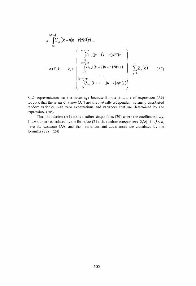
Such representation has the advantage because from a structure of expression (A6) follows, that the terms of a sum (A7) are the mutually independent normally distributed random variables with zero expectations and variances that are determined by the expressions (A6).

Thus the relation (A4) takes a rather simple form (20) where the coefficients a,, I I n? 2 77, are calculated by the formulae (21) the random components Z,(k), 1 5.j 5 n, have the structure (A6) and their variances and covariances are calculated by the formulae (22) - (24)

505

506