the probability that the number of points on the jacobian...
TRANSCRIPT
Proc. London Math. Soc. (3) 104 (2012) 1235–1270 C�2012 London Mathematical Societydoi:10.1112/plms/pdr063
The probability that the number of points on the Jacobianof a genus 2 curve is prime
Wouter Castryck, Amanda Folsom, Hendrik Hubrechts and Andrew V. Sutherland
Abstract
In 2000, Galbraith and McKee heuristically derived a formula that estimates the probability thata randomly chosen elliptic curve over a fixed finite prime field has a prime number of rationalpoints. We show how their heuristics can be generalized to Jacobians of curves of higher genus.We then elaborate this in genus g = 2 and study various related issues, such as the probabilityof cyclicity and the probability of primality of the number of points on the curve itself. Finally,we discuss the asymptotic behavior for g → ∞.
1. Introduction and overview
1.1. The Galbraith–McKee conjecture: elliptic curves
Galbraith and McKee [17] studied the probability that a randomly chosen elliptic curve overa finite prime field has a prime number of rational points. They conjectured the following. Fora prime number p > 3, let P1(p) be the probability that a uniformly randomly chosen integerin the Hasse interval [p + 1− 2
√p, p + 1 + 2
√p] is prime. Let P2(p) be the probability that
the elliptic curve defined by y2 = x3 + Ax + B, for a uniformly randomly chosen pair (A,B)in the set
HAB = {(A,B) ∈ F2p|4A3 + 27B2 �= 0},
has a prime number of rational points (including the point at infinity).
Conjecture 1 (Galbraith–McKee [17, Conjecture A]). Define
cp =23·∏�>2
(1− 1
(�− 1)2
)·
∏�|p−1,�>2
(1 +
1(� + 1)(�− 2)
),
where the products are over all primes � satisfying the stated conditions. Then
limp→∞(P2(p)/P1(p)− cp) = 0.
The constant cp lies between 0.44010 and 0.61514. In general, the conjecture predicts thatelliptic curves are about half as likely to have prime orders as one might expect.
The study of the probability of primality is partly motivated by elliptic curve cryptography.For an elliptic curve over a finite field to be suitable as the underlying group for Diffie–Hellmankey exchange, its number of rational points is preferably prime (although small cofactors areoften tolerated). In practice, a ‘good’ elliptic curve is often found by repeatedly counting thenumber of rational points on randomly chosen elliptic curves, for example using the SEA
Received 22 January 2011; published online 6 February 2012.
2010 Mathematics Subject Classification 11N05, 11G10, 11G20.
The research of the first and the third author was financially supported by F.W.O.-Vlaanderen. The secondauthor is grateful for the support of National Science Foundation grant DMS 1049553.

1236 W. CASTRYCK ET AL.
algorithm [31], until a prime number is hit. The above conjecture predicts that this processworks slightly worse than one would naıvely assume.
Galbraith and McKee provided both experimental support and heuristic evidence in favorof Conjecture 1. Their main argument uses the Hurwitz–Kronecker class number formula,which counts bivariate quadratic forms up to equivalence. A second argument estimates theprobability of primality by naıvely multiplying the expected probabilities of being coprime to2, 3, 5, 7, 11, . . . For elliptic curve orders, these expected probabilities were devised by Lenstra[25, Proposition 1.14]. When taking the quotient of the resulting estimates for P2(p) and P1(p),one exactly finds cp. A reasoning of this kind had already been made by Koblitz [23, p. 160] inthe dual setting where one fixes an elliptic curve over Q and reduces it modulo varying primes,a similar discussion on the case where one fixes a CM-curve of genus 2 over Q can be readin Weng’s thesis [35, Section 5.2]. Galbraith and McKee called their second heuristics ‘notvery honest’, however, due to subtleties reflected in Mertens’ theorem. We will discuss these inSection 3.
1.2. Genus 2 curves
Nonetheless, and this may be thought of as an underlying meta-conjecture, these secondheuristics work very well in practice, as is confirmed experimentally in Section 11. Moreover,they seem more flexible towards generalizing Conjecture 1 to Jacobians of curves of highergenus, which have also been proposed for use in cryptography. The required analoguesof Lenstra’s theorem are provided by a recursive formula due to Achter and Holden [3,Lemma 3.2], which we turn into a closed expression in Section 5.
In this article, we elaborate this for curves of genus 2, which is the most relevant case forcryptography. We derive the following conjecture. For a prime number p > 2, let P1(p) be theprobability that a uniformly randomly chosen integer in the Hasse–Weil interval
[(√
p− 1)4, (√
p + 1)4]
is prime. Let P2(p) be the probability that the Jacobian of the genus 2 curve defined byy2 = f(x), for a randomly chosen polynomial f(x) in the set
H6 = {f(x) ∈ Fp[x]|f(x) square-free of degree 6},has a prime number of rational points.
Conjecture 2 (see Section 6). Define
cp =3845·∏�>2
(1− �2 − �− 1
(�2 − 1)(�− 1)2
)·
∏�|p−1,�>2
(1 +
�4 − �3 − �− 2(�3 − 2�2 − � + 3)(�2 + 1)(� + 1)
),
where the products are over all primes � satisfying the stated conditions. Then
limp→∞(P2(p)/P1(p)− cp) = 0.
We implicitly assume that P1(p) �= 0 for all p, which is an open problem in its own (see[8, Section 2.2] for a related discussion). The constant cp lies between 0.63987 and 0.79890.Summarizing, in genus 2, prime order Jacobians are also slightly disfavored, but to a lesserextent than in genus 1.
1.3. Averaging over p
By averaging cp over all primes p, it becomes meaningful to measure the prime-disfavoringbehavior by a single constant. For elliptic curves, this gives the following lemma.
THE PROBABILITY THAT A GENUS 2 JACOBIAN HAS PRIME ORDER 1237
Lemma 1 (see Section 3). For each prime p > 3, let cp be as in Conjecture 1. Then
cp = limn→∞
1π(n)
∑3<p�n
cp =∏
�
(1− �2 − �− 1
(�2 − 1)(�− 1)2
)≈ 0.50517.
Here, π is the prime-counting function, and the product is over all primes �.
This confirms a constant obtained by Koblitz [23, p. 160] and subsequently verified by Balog,Cojocaru and David [5, Theorem 1]. In genus 2, the average reads as follows.
Lemma 2 (see Section 6). For each prime p > 2, let cp be as in Conjecture 2. Then
cp = limn→∞
1π(n)
∑2<p�n
cp =∏
�
(1− �6 − 2�5 + 3� + 1
(�2 − 1)2(�2 + 1)(�− 1)2
)≈ 0.69464,
where again the product is over all primes �.
1.4. Imposing a rational Weierstrass point
Instead of using H6, we can choose f(x) uniformly at random from the set
Hm5 = {f(x) ∈ Fp[x]|f(x) monic and square-free of degree 5}.
This situation matches better with common cryptographic practice. However, it alters thenotion of taking a random genus 2 curve, since here one imposes the existence of a rationalWeierstrass point. As before, for each prime p > 2, let P1(p) be the probability that a uniformlyrandomly chosen integer in the Hasse–Weil interval [(
√p− 1)4, (
√p + 1)4] is prime, but now
let P2(p) be the probability that a random genus 2 curve, in the above sense, has a Jacobianwith a prime number of rational points.
Conjecture 3 (see Section 7). Let cp be as in Conjecture 2. Then
limp→∞
(P2(p)/P1(p)− 9
19cp
)= 0.
The constant 919cp lies between 0.30309 and 0.37843, so prime orders become dramatically
less probable. This is entirely due to the fact that the probability of having rational 2-torsionincreases from 26
45 to 45 . In Section 7, we will illustrate why for odd �, the expected probability
of having rational �-torsion is most likely unaffected.Averaging 9
19cp over all primes p as in Section 1.3 gives approximately 0.32904 (that is, 919
times the constant of Lemma 2).
1.5. The number of points on the curve itself
We can also estimate the probability that the number of rational points on the curve itself,rather than its Jacobian, is prime. For each prime p > 2 and with f(x) chosen uniformly atrandom fromH6, let P2(p) be the probability that the non-singular complete model of y2 = f(x)has a prime number of rational points. Let P1(p) be the probability that an integer, chosenuniformly at random from the Hasse–Weil interval
[p + 1− 4√
p, p + 1 + 4√
p],
1238 W. CASTRYCK ET AL.
is prime. For � �= p prime, define
a�,p := #{(x, y) ∈ F×� × (F×
� \{−p}) | (x + y/x)(1 + p/y) = p + 1},β�,p := (�− 1)(�5 − �3 + 2)− a�,p −
{(�3 − 1) if p ≡ −1 mod �,0 otherwise.
Conjecture 4 (see Section 8). Define
cp =3845
∏�>2� �=p
� · β�,p
(�4 − 1)(�2 − 1)(�− 1),
where the product is over all primes satisfying the stated conditions. Then
limp→∞(P2(p)/P1(p)− cp) = 0.
The constant cp lies between 0.79605 and 0.86548, with an estimated average (in the senseof Section 1.3) of cp ≈ 0.83376 . When switching to Hm
5 instead of H6, the leading factor 3845
should be replaced by 1615 . The resulting constant cp lies between 1.00553 and 1.09323, with an
estimated average of cp ≈ 1.05317, so prime orders actually become slightly favoured.
1.6. The probability of cyclicity
Using similar heuristics, one can estimate for each prime p > 2 the probability P (p, 2) thatthe group of rational points on the Jacobian of the curve defined by y2 = f(x), with f(x)chosen uniformly at random from H6, is cyclic. This is done by considering for each prime �the corresponding probability for the �-torsion subgroup, and then taking the product.
For elliptic curves, one recovers a formula that was proven by Vladut. Let P (p, 1) be theprobability that the group of rational points on a randomly chosen elliptic curve over Fp (asin Section 1.1) is cyclic. Then we have the following theorem.
Theorem 1 (Vladut [34, Theorem 6.1]). For each prime p, define
cp =∏
�|p−1
(1− 1
�(�2 − 1)
),
where the product is over all primes satisfying the stated condition. Then
limp→∞(P (p, 1)− cp) = 0.
The constant cp is contained in [0.78816, 0.83334], with an average (in the sense of Section 1.3)of cp ≈ 0.81375. In genus 2, the same reasoning gives the following conjecture.
Conjecture 5 (see Section 9). For each prime p, define
cp =151180·
∏�>2,��p−1
(1− 1
�(�2 − 1)(�− 1)
)·
∏�>2,�|p−1
�8 − �6 − �5 − �4 + �2 + � + 1�2(�4 − 1)(�2 − 1)
,
where the products are over all primes � satisfying the stated conditions. Then
limp→∞(P (p, 2)− cp) = 0.

THE PROBABILITY THAT A GENUS 2 JACOBIAN HAS PRIME ORDER 1239
The constant cp is contained in the interval [0.79356, 0.81918], with an average value cp ≈0.80883. If we replaceH6 byHm
5 , then the leading factor should be replaced by 3760 , in which case
the constant cp is contained between 0.58335 and 0.60218, with an average value cp ≈ 0.59457.
1.7. Extension fields
Fix a prime number p. Consider the alternative setup of finite fields Fpk of growing extensiondegree k over Fp. For g ∈ {1, 2}, let P1(k, g) be the probability that a uniformly randomlychosen integer in the Hasse interval [(
√pk − 1)2g, (
√pk + 1)2g] is prime. Let P2(k, g) be the
probability that the Jacobian of the (hyper)elliptic curve defined by y2 + h(x)y = f(x), wherethe pair (h, f) is chosen from
Hg+1,2g+2 = {(f, h) ∈ Fpk [x]× Fpk [x]|deg h � g + 1,deg f = 2g + 2,
y2 + h(x)y = f(x) has geometric genus g}uniformly at random, has a prime number of Fpk -rational points.
Then we have the following.
Conjecture 6 (see Section 10). Let
ck = μp ·∏�>2
(1− 1
(�− 1)2
)·
∏�|pk−1,�>2
(1 +
1(� + 1)(�− 2)
),
where the products are over all primes � satisfying the stated conditions, and μp = 0 if p = 2versus μp = 2
3 if p > 2. Then
limk→∞
(P2(k, 1)/P1(k, 1)− ck) = 0.
If p > 2, the formula for ck closely matches the formula from cp from Conjecture 1, withpk − 1 in place of p− 1, and takes values between 0.44010 and 0.61514. For p = 2 we haveck = 0. In genus 2, the estimate reads as follows.
Conjecture 7 (see Section 10). Let
ck = μp ·∏�>2
(1− �2 − �− 1
(�2 − 1)(�− 1)2
)·
∏�|pk−1,�>2
(1 +
�4 − �3 − �− 2(�3 − 2�2 − � + 3)(�2 + 1)(� + 1)
),
where the products are over all primes � satisfying the stated conditions, and μp = 23 if p = 2
versus μp = 3845 if p > 2. Then
limk→∞
(P2(k, 2)/P1(k, 2)− ck) = 0.
Again for p > 2, the formula for ck matches the formula for cp in Conjecture 2 and takesvalues between 0.63987 and 0.79890. If p = 2, then ck lies between 0.50516 and 0.63071.
It is possible to average the above over k, where the result will depend on the multiplicativeorders of p modulo the various �. Also, one can adapt Conjectures 6 and 7, and in fact any ofthe conjectures stated above, to the mixed case of just considering finite fields Fq of growingcardinality.
1.8. Asymptotics for growing genus
Instead of elaborating similar, increasingly complicated formulas for higher genera g, weconclude with an analysis of the asymptotic behavior for g →∞. This may be of interestto people studying analogues of the Cohen–Lenstra heuristics [11, 24] in the case of function
1240 W. CASTRYCK ET AL.
fields, though we will not push this connection. Note that due to computational limitations,the conjectures below are no longer supported by experimental evidence and rely purely on theconjectured validity of our heuristic derivation.
For every prime number p > 2 and every integer g � 1, let P1(p, g) be the probability thata uniformly randomly chosen integer in the Hasse–Weil interval
[(√
p− 1)2g, (√
p + 1)2g]
is prime. Let P2(p, g) be the probability that the Jacobian of the genus g curve defined byy2 = f(x), for a randomly chosen polynomial f(x) in the set
H2g+2 = {f(x) ∈ Fp[x]| f(x) square-free of degree 2g + 2},has a prime number of rational points.
Then we have the following theorem.
Theorem 2 (see Section 6). limp,g→∞ P2(p, g) = 0.
Theorem 2 holds because the probability of having rational 2-torsion tends to 1 as g →∞.However, this is a hyperelliptic phenomenon. The limiting behavior becomes more interestingif instead one defines P2(p, g) as the probability that the Jacobian of a random genus g curveover Fp (for example, chosen from the set
Mg = {curves of genus g over Fp}/ ∼=Fp
uniformly at random, note that Mg is typically not well-understood) has a prime number ofrational points. In this case, we expect the following conjecture.
Conjecture 8 (see Section 6). Define
cp =1∏∞
j=2 ζ(j)·∏
�|p−1
∞∏j=1
�2j
�2j − 1,
where ζ is Riemann’s zeta function and the product is over all primes � satisfying the statedcondition. Then
limp,g→∞(P2(p, g)/P1(p, g)− cp) = 0.
Again, we implicitly assume that P1(p, g) is nowhere zero. The constant cp lies in the interval[∏∞j=1(2
2j/(22j − 1))∏∞j=2 ζ(j)
,1∏∞
j=1 ζ(2j + 1)
]⊂ [0.63287, 0.79353].
In other words, the prime-disfavoring effect persists as the genus grows. It even becomes slightlymore manifest than in genus 2. A more detailed analysis shows that the effect alternatelystrengthens and weakens as the genus becomes odd and even, respectively. As in Section 1.3,one can average cp over all primes p > 2, yielding a constant cp ≈ 0.68857.
Similarly, for every prime number p > 2 and every integer g � 1, let P (p, g) be the probabilitythat the rational points of the Jacobian of the (hyper)elliptic curve y2 = f(x), with f(x) pickedfrom H2g+2 uniformly at random, constitute a cyclic group.
Then we have the following theorem.
Theorem 3 (see Section 9). limp,g→∞ P (p, g) = 0.

THE PROBABILITY THAT A GENUS 2 JACOBIAN HAS PRIME ORDER 1241
Again, this is a hyperelliptic phenomenon due to 2-torsion issues. If instead we define P (p, g)to be the probability that a curve chosen fromMg uniformly at random has a cyclic Jacobian,then we expect the following conjecture.
Conjecture 9 (see Section 9). Define
cp =1∏∞
j=2 ζ(j)·∏
�|p−1
∞∏j=1
�2j
�2j − 1·∏
��p−1
(1 +
1�(�− 1)
),
where ζ is Riemann’s zeta function and the product is over all primes � satisfying the statedconditions. Then
limp,g→∞(P (p, g)− cp) = 0.
Now the constant cp lies in the interval[1∏∞
j=1 ζ(2j + 1),
∏∞j=1(2
2j/(22j − 1) ·∏�>2(1 + 1/�(�− 1))∏∞j=2 ζ(j)
]⊂ [0.79352, 0.82004],
with an average (in the sense of Section 1.3) of cp ≈ 0.80924.
2. Common notions of randomness
By a randomly chosen (hyper)elliptic curve of genus g � 1 over a finite field Fq of oddcharacteristic, we will usually mean the non-singular complete model of a curve y2 = f(x),where f is chosen from
H2g+2 = {f(x) ∈ Fq[x]|f(x) is square-free and deg f = 2g + 2}uniformly at random.
Alternatively, one could take the curve uniformly at random from
Mhypg = {(hyper)elliptic genus g curves over Fq}/ ∼=Fq
.
This randomness notion may be preferred from a theoretical point of view. It is fundamentallydifferent from our first, in the sense that the map
H2g+2 −→Mhypg : f �−→ [y2 = f(x)]
is not uniform. For small q, it does not even need to be surjective. Therefore, the probabilityof having a certain geometric property may change when moving from one notion to the other.However, as q gets bigger and bigger, the change becomes negligible. More precisely, for q →∞(g fixed), the proportion of elements of Mhyp
g having q(q2 − 1)(q − 1)/2 pre-images in H2g+2
tends to 1. This can be elaborated following [27, Section 1]. Note that, despite the availabilityof a complete classification of (hyper)elliptic curves up to Fq-isomorphism [27, Section 2], theset Mhyp
g is quite cumbersome to work with.Another setup, which is, for example, used in [2, Theorem 3.1], is to take f uniformly at
random from
Hm2g+2 = {f(x) ∈ Fq[x]| f(x) is monic, square-free and deg f = 2g + 2},
instead of H2g+2. Again, this is different from either of the above notions. For small q, theremay exist curves having a model in H2g+2 that do not have a model in Hm
2g+2. But again, asq →∞ (g fixed), the difference dissolves. Indeed, consider the set
S2g+2 = {(f, α, β) ∈ H2g+2 × Fq × F×q |f(α) = β2}.
1242 W. CASTRYCK ET AL.
Then we have a map
S2g+2 −→ Hm2g+2 : (f, α, β) �−→ β−2x2g+2f(1/x + α),
which respects the isomorphism class of the corresponding curve, and which is onto and q(q −1)-to-1. Therefore, taking f uniformly at random from Hm
2g+2 and using the f of a uniformlyrandomly chosen (f, α, β) ∈ S2g+2 give rise to equivalent randomness notions. On the otherhand, the map
S2g+2 −→ H2g+2 : (f, α, β) �−→ f
is asymptotically uniform, since every f ∈ H2g+2 will have q + O(√
q) pre-images by the Hasse–Weil bound. This proves the claim.
In Section 10, we will allow char Fq = 2 and use curves of the form y2 + h(x)y = f(x) with(f, h) chosen from
Hg+1,2g+2 = {(f, h) ∈ Fq[x]× Fq[x]|deg h � g + 1,deg f = 2g + 2,
y2 + h(x)y = f(x) has geometric genus g}uniformly at random. Again, it is easy to show that if 2 � q, the completing-the-square mapHg+1,2g+2 → H2g+2 is essentially uniform.
In this article, we will always consider statistical behavior for q →∞. In particular, thevalidity of all statements below involving randomly chosen curves in the sense of H2g+2
is preserved when switching to either of the above alternatives, and vice versa. Somestatements involve error terms, so in fact a more careful analysis is needed; we omit thedetails.
The picture does alter, however, when one takes f uniformly at random from
H2g+1 = {f ∈ Fq[x]|f(x) is square-free and deg f = 2g + 1}.While this setting is often preferred in practice, this influences the story as soon as g � 2, sinceit induces the existence of a rational Weierstrass point. We will study this effect in detail forg = 2 in Section 7. On the other hand, writing
Hm2g+1 = {f ∈ Fq[x]|f(x) is monic, square-free and deg f = 2g + 1},
the geometry-preserving map
H2g+1 −→ Hm2g+1 : f �−→ α2gf(x/α) (where α = lc(f))
is onto and (q − 1)-to-1. Therefore, H2g+1 and Hm2g+1 can be interchanged in any probability
statement below. If g = 1 and moreover 3 � q, then this also accounts for
HAB = {(A,B) ∈ F2q|4A3 + 27B2 �= 0},
since the completing-the-cube map H3 → HAB is uniform.Note that the sets H2g+2,Hm
2g+2,Hg+1,2g+2,H2g+1,Hm2g+1,Mhyp
g and HAB depend on q,while this is not included in the notation for the sake of readability. However, it will alwaysbe clear from the context which q is used (it will typically be the prime number p underconsideration).
3. Heuristic framework
For prime numbers p > 3 and � �= p, let P (p, �) be the probability that the elliptic curve EAB
defined by y2 = x3 + Ax + B, for a randomly chosen pair (A,B) in the set HAB , has � dividingits number of rational points (including the point at infinity).
THE PROBABILITY THAT A GENUS 2 JACOBIAN HAS PRIME ORDER 1243
Theorem 4 (Lenstra). There exist C1, C2 ∈ R>0, such that∣∣∣∣P (p, �)− �
�2 − 1
∣∣∣∣ � C1�/√
p if � | p− 1 and∣∣∣∣P (p, �)− 1�− 1
∣∣∣∣ � C2�/√
p if � � p− 1
for all pairs of distinct primes p, � with p > 3.
Proof. See [25, Proposition 1.14], to which we refer for explicit estimates of the Ci.
We can now describe and discuss in more detail Galbraith and McKee’s second heuristicargument supporting Conjecture 1. This is the type of reasoning behind all of our conjectures.Let �(p) be the largest prime for which �(p) � √p + 1. Let n be an integer chosen uniformly atrandom from the Hasse interval, and let η be #EAB(Fp). The aim was to estimate the ratioP2(p)/P1(p), where P1(p) and P2(p) are as in Section 1.1. It can be rewritten as
P (2 � η and 3 � η and 5 � η and . . . and �(p) � η)P (2 � n and 3 � n and 5 � n and . . . and �(p) � n)
.
A first heuristic step is to approximate the above by
P (2 � η)P (3 � η)P (5 � η) . . . P (�(p) � η)P (2 � n)P (3 � n)P (5 � n) . . . P (�(p) � n)
.
A second heuristic step is then to estimate P (� � η) by
1− 1�− 1
if � � p− 1, and 1− �
�2 − 1if � | p− 1
(following Theorem 4), and P (� � n) by
1− 1�.
One finds that
c′p =
∏��p−1(1− 1/(�− 1)) ·∏�|p−1(1− �/(�2 − 1))∏
(1− 1/�),
where the products are over all primes � � �(p) satisfying the stated conditions. Rearrangingthe expression shows that
limp→∞(cp − c′p) = 0,
where cp is the factor appearing in Conjecture 1.It is tempting to validate the heuristics using an independence argument based on the Chinese
Remainder Theorem (for n) and Howe’s generalization of Lenstra’s theorem (for η, see [19]).However, this is too naıve. By Mertens’ theorem and the Prime Number Theorem, we have∏
��√p+1
(1− 1
�
)≈ 2e−γ
log p≈ 2e−γP1(p).
Here, γ ≈ 0.57722 is the Euler–Mascheroni constant (2e−γ ≈ 1.12292). For the heuristics to bejustified, we should therefore have∏
��p−1,��√p+1
(1− 1
�− 1
)·
∏�|p−1,��√
p+1
(1− �
�2 − 1
)≈ 2e−γP2(p).

1244 W. CASTRYCK ET AL.
With this in mind, the heuristics becomes very subtle: why would both naıve estimates be“equally wrong”, in the words of Galbraith and McKee? We cannot give a satisfying answer, butnote the following. (i) The constant 2e−γ , which reflects the ignored dependency between beingdivisible by distinct primes, is accumulated in the tail of the product, with respect to whichη and n behave much alike. Stated alternatively, the ‘local ratios’ P (� � η)/P (� � n) convergequickly to 1. By considering cp as the limiting product of these local ratios, rather than theratio of two diverging products, one gets a more comfortable underpinning of the conjecturedheuristics. (ii) The heuristics are supported by Galbraith and McKee’s first argument in favorof Conjecture 1, which uses different methods (namely, the analytic Hurwitz–Kronecker classnumber formula). (iii) As far as computationally feasible, the conjectures that we obtainassuming this principle are confirmed by experiment in Section 11. (iv) The constant fromLemma 1 provably appeared in the dual setting of a fixed elliptic curve over Q reduced modulovarying primes p (see [5, Theorem 1]).
We complete this section with a proof of Lemma 1.
Proof of Lemma 1. First, let us give a heuristic derivation. Let � be a prime number. ByDirichlet’s theorem, the proportion of primes p satisfying � | p− 1 is 1/(�− 1). Averaging outLenstra’s result then gives
P (� | η) ≈ 1�− 1
�
�2 − 1+
�− 2�− 1
1�− 1
=�2 − 2
(�2 − 1)(�− 1).
SoP (� � η)P (� � n)
≈ 1− �2 − �− 1(�2 − 1)(�− 1)2
,
and applying the above heuristics yields the requested formula.To make the argument precise, pick any ε > 0. It is easy to see that there is a uniform bound
L such that |cLp − cp| < ε/3 for all p, where cL
p is defined as in Conjecture 1, but with theproduct restricted to primes � that do not exceed L, and such that, similarly,∣∣∣∣∣∣
∏��L
(1− �2 − �− 1
(�2 − 1)(�− 1)2
)−∏
�
(1− �2 − �− 1
(�2 − 1)(�− 1)2
)∣∣∣∣∣∣ < ε/3.
However, by the Dirichlet equidistribution of primes, and because we are taking finite productsnow, there is an N such that n � N implies∣∣∣∣∣∣
1π(n)− 2
∑3<p�n
cLp −
∏��L
(1− �2 − �− 1
(�2 − 1)(�− 1)2
)∣∣∣∣∣∣ < ε/3.
Combining the three bounds concludes the proof.
4. The random matrix model
4.1. The genus 1 case
Lenstra’s Theorem 4 can be understood from the following random matrix point of view. LetFq be a finite field. Let N be a positive integer coprime to q, and consider the set
GL(q)2 (Z/(N)) = {M ∈ GL2(Z/(N))|det M = q}.
This set is acted upon by GL2(Z/(N)), by conjugation. To any elliptic curve E/Fq, wecan unambiguously associate an orbit of this action by collecting the matrices of qth power
THE PROBABILITY THAT A GENUS 2 JACOBIAN HAS PRIME ORDER 1245
Frobenius, considered as an endomorphism of the Z/(N)-module E[N ] of N -torsion points,with respect to all possible bases. Denote this orbit by FE .
Take char Fq > 3. For any union of orbits C ⊂ GL(q)2 (Z/(N)), let P (FE ⊂ C) denote the
probability that the orbit associated to the elliptic curve y2 = x3 + Ax + B, where (A,B) ∈ Fq
is chosen from HAB uniformly at random, is contained in C.
Principle 1. There exist C1 ∈ R>0 and c ∈ Z>0, such that∣∣∣∣∣P (FE ⊂ C)− #C#GL
(q)2 (Z/(N))
∣∣∣∣∣ � C1Nc/√
q
for all choices of q, N and C as above.
We use the word ‘Principle’, because, to our knowledge, no complete proof of this statementhas been published in the literature. Nevertheless, it is commonly accepted and extensivelyconfirmed by experiment. It is generally believed to follow from the work of Katz and Sarnak[20, Theorem 9.7.13]. A strategy of proof was communicated to us by Katz, and essentiallymatches with the approach of Achter [2, Theorem 3.1], who proved Principle 1 under certainmild restrictions on q and N (using c = 3). However, a more classically flavored proof ofPrinciple 1 can be obtained by applying Chebotarev’s density theorem [13, Proposition 6.4.8]to the function field extension Fq(j) ⊂ Fq(ζN )(j) ⊂ Fq(ζN )(X(N)), where ζN is a primitiveNth root of unity, and the latter extension corresponds to the modular cover X(N)→ X(1),which is known to be defined over Fq(ζN ). This approach has recently been elaborated in apreprint of Castryck and Hubrechts [9].
Principle 1 indeed allows one to rediscover the asymptotics of Theorem 4, by counting thematrices M ∈ GL(p)
2 (F�) satisfying p + 1− Tr(M) = 0. We leave this as an exercise.
4.2. The general case
Let Fq and N be as before, and let Fq be an algebraic closure of Fq. Let C/Fq be a completenon-singular curve of genus g � 1 and denote by A = Jac(C) its Jacobian. Then qth powerFrobenius defines an endomorphism of the 2g-dimensional Z/(N)-module A[N ] of N -torsionpoints on A. Instead of considering all bases, we can make a more canonical choice by restrictingto symplectic bases. We briefly review how this works.
We employ the following notation and terminology. For any n ∈ N, In denotes the n× nidentity matrix, and Ω denotes the 2g × 2g matrix(
0 Ig
−Ig 0
).
The group
Sp2g(Z/(N)) = {M ∈ GL2g(Z/(N))|tMΩM = Ω}is called the group of symplectic 2g × 2g matrices, and
GSp2g(Z/(N)) = {M ∈ GL2g(Z/(N))|∃ d ∈ Z/(N) such that tMΩM = dΩ},is referred to as the group of symplectic similitudes. It is naturally partitioned into the sets
GSp(d)2g (Z/(N)) = {M ∈ GL2g(Z/(N))|tMΩM = dΩ},

1246 W. CASTRYCK ET AL.
with d ranging over (Z/(N))×. An element of GSp(d)2g (Z/(N)) is called d-symplectic. Note
that 1-symplectic and symplectic are synonymous. A classical trick using the Pfaffian showsthat the determinant of a symplectic matrix is 1. Hence the determinant of a d-symplecticmatrix is dg.
Symplectic matrices pop up in the study of skew-symmetric, non-degenerate bilinear pairingson, in our case, 2g-dimensional (Z/(N))-modules. Such pairings are often called symplecticforms. For any choice of basis, one can consider the standard symplectic form 〈·, ·〉, defined bythe rule
〈v, w〉 = tvΩw.
Given any symplectic form, one can always choose a basis with respect to which it becomes thestandard symplectic form: such a basis is called a symplectic basis or a Darboux basis. If oneswitches between two symplectic bases corresponding to the same symplectic form, the matrixof base change is symplectic, and conversely.
Now for each primitive Nth root of unity ζN ∈ Fq, the Weil pairing
eN : A[N ]×A[N ] −→ 〈ζN 〉,when composed with the (non-canonical) map
〈ζN 〉 −→ Z/(N) : ζiN �−→ i,
is a skew-symmetric and non-degenerate bilinear pairing on A[N ]. A corresponding symplecticbasis P1, . . . , Pg, Q1, . . . , Qg is characterized by the properties
eN (Pi, Qj) = ζδij
N , eN (Pi, Pj) = eN (Qi, Qj) = 1
for all i, j ∈ {1, . . . , g}, where δij is the Kronecker symbol. Because of the Gal(Fq, Fq)-invarianceof the Weil pairing, one has that
eN (P σ, Qσ) = eN (P,Q)q,
where P and Q are arbitrary points of A[N ] and σ is qth power Frobenius. Then bilinearityimplies that the matrix F of σ with respect to P1, . . . , Pg, Q1, . . . , Qg satisfies
tFΩF = qΩ,
that is, F is q-symplectic.As mentioned above, a different choice of symplectic basis yields a matrix obtained from
F by Sp2g(Z/(N))-conjugation. Next, if ζN is replaced by another Nth root of unity ζjN ,
j ∈ (Z/(N))×, then P1, . . . , Pg, [j]Q1, . . . , [j]Qg is a symplectic basis, and the matrix ofFrobenius is djFd−1
j , where
dj =(
Ig 00 jIg
).
Since Sp2g(Z/(N)) and the matrices dj generate GSp2g(Z/(N)), we conclude that we canunambiguously associate to C an orbit of GSp(q)
2g (Z/(N)) under GSp2g(Z/(N))-conjugation.We are now ready to formulate the hyperelliptic curve analogue of Principle 1. Let char
Fq > 2 and g � 1. For any union of GSp2g(Z/(N))-orbits C ⊂ GSp(q)2g (Z/(N)), let P (Ff ⊂ C)
denote the probability that the orbit associated to the complete non-singular model of the(hyper)elliptic curve y2 = f(x), where f(x) ∈ Fq[x] is chosen from H2g+2 uniformly at random,is contained in C.
THE PROBABILITY THAT A GENUS 2 JACOBIAN HAS PRIME ORDER 1247
Principle 2. There exist C1 ∈ R>0 and c ∈ Z>0, such that∣∣∣∣∣P (Ff ⊂ C)− #C#GSp(q)
2g (Z/(N))
∣∣∣∣∣ � C1Nc/√
q
for all choices of q, N and C as above, provided that N is odd as soon as g > 2.
The condition N odd is due to the fact that we restrict to hyperelliptic curves, which assoon as g > 2 behave non-randomly with respect to 2-torsion (see Section 6). If instead weconsidered Jacobians of arbitrary curves (for example, in the sense of Section 1.8), we expectthat this condition could be dropped.
Again we use the word ‘Principle’, because no complete proof of this statement has appearedin the literature to date. But again, this presumably follows from the work of Katz and Sarnak[20, Theorem 9.7.13], as elaborated by Achter [2, Theorem 3.1] under mild restrictions on q andN . In his case, the exponent reads c = 2g2 + g. Achter’s result is sufficiently general for manyof our needs below. In particular, it is sufficient for generalizing Theorem 4 to (hyper)ellipticcurves of arbitrary genus g � 1, which is done in Section 6. Also note that Achter uses Hm
2g+2
rather than H2g+2.
5. Counting matrices with eigenvalue 1
For use in Sections 6 and 9, we study the following general question: given a prime powerq, a prime � � q, an integer g � 0 and d ∈ {0, . . . , 2g}, what is the proportion P(q, �, g, d) ofmatrices in GSp(q)
2g (F�) for which the eigenspace for eigenvalue 1 is d-dimensional? Lemma 3transfers this question to the classical groups Sp2g(F�) and GLg(F�). Let PSp(�, g, d) be theproportion of matrices in Sp2g(F�) having a d-dimensional eigenspace for eigenvalue 1, and letPGL(�, g, d) be the corresponding proportion for the general linear group GLg(F�), where ofcourse PGL(�, g, d) = 0 as soon as d > g. We include g = 0 because of the recursive nature of thearguments below. In this, we assume that GSp(q)
0 (F�) = Sp0(F�) = GL0(F�) contains a uniquematrix and that its 1-eigenspace is 0-dimensional. In particular, P(q, �, 0, 0) = PSp(�, 0, 0) =PGL(�, 0, 0) is understood to be 1.
Lemma 3. If q ≡ 1 mod �, then P(q, �, g, d) = PSp(�, g, d). If q �≡ 1 mod �, thenP(q, �, g, d) = PGL(�, g, d).
Proof. The first statement is a tautology. So, assume that q �≡ 1 mod �. We follow ideas ofAchter and Holden [3, Lemma 3.1], which in turn build upon work of Chavdarov [10].
First, for r = 0, . . . , g, let S(q, �, r, d) be the subset of GSp(q)2r (F�) consisting of those matrices
having characteristic polynomial (x− 1)r(x− q)r and whose 1-eigenspace has dimensiond. Similarly, let SGL(�, r, d) be the subset of GLr(F�) consisting of the matrices havingcharacteristic polynomial (x− 1)r and whose 1-eigenspace has dimension d.
We will prove that
#S(q, �, r, d) =#Sp2r(F�)#GLr(F�)
·#SGL(�, r, d). (1)
By Jordan–Chevalley decomposition, every element B ∈ S(q, �, r, d) can be uniquely writtenas the commuting product of a semisimple matrix Bs and a unipotent matrix Bu. Necessarily,Bs ∈ GSp(q)
2r (F�) has as characteristic polynomial (x− 1)r(x− q)r and Bu ∈ Sp2r(F�) hasas characteristic polynomial (x− 1)2r. By [10, Lemma 3.4], two such matrices Bs mustbe conjugated by an element of Sp2r(F�). It follows that for fixed Bs, the number of
1248 W. CASTRYCK ET AL.
corresponding instances of B in S(q, �, r, d) is always the same. Since one instance of Bs isdiag(1, 1, . . . , 1, q, q, . . . , q), whose centralizer in Sp2r(F�) equals
{(M 00 t(M−1)
)∣∣∣∣M ∈ GLr(F�)}
,
the number of possibilities for Bs is (#Sp2r(F�))/(#GLr(F�)), and for each Bs there areSGL(�, r, d) appropriate choices for Bu. The claim follows.
Now, let T (q, �, g, d) be the set of matrices of GSp(q)2g (F�) having a d-dimensional 1-eigenspace,
thus #T (q, �, g, d) = P(q, �, g, d) ·#Sp2g(F�). We will count the elements M ∈ T (q, �, g, d)separately for each value of r, the order of vanishing at 1 of the characteristic polynomial fM ofM . To M, one can associate a decomposition of the standard symplectic space F2g
� , 〈·, ·〉 of theform U2r ⊕ V2(g−r), where U2r and V2(g−r) are M -invariant symplectic subspaces of dimensions2r and 2(g − r), respectively, satisfying fM |U2r
= (x− 1)r(x− q)r and fM |V2(g−r)(1) �= 0. Then
#T (q, �, g, d) =g∑
r=0
#Sp2g(F�)#Sp2r(F�) ·#Sp2(g−r)(F�)
·#S(q, �, r, d) ·#T (q, �, g − r, 0),
where the first factor corresponds to the number of ways of decomposing F2g� , 〈·, ·〉, the second
factor counts the number of possible actions of M on U2r and the third factor counts thenumber of actions of M on V2(g−r). We conclude that
P(q, �, g, d) =g∑
r=0
#S(q, �, r, d)#Sp2r(F�)
·P(q, �, g − r, 0). (2)
Along with
g∑d=0
P(q, �, g, d) = 1, (3)
one sees that, given the values #S(q, �, r, d), the recursive equation (2) determines allP(q, �, g, d) by induction on g: first one determines P(q, �, g, 1), . . . ,P(q, �, g, g), during whichone should use that #S(q, �, 0, d) = 0 as soon as d > 0, and then one uses (3) to obtainP(q, �, g, 0).
The statement then follows by noting that one similarly has
PGL(�, g, d) =g∑
r=0
#SGL(�, r, d)#GLr(F�)
·PGL(�, g − r, 0),
along with the same initial conditions. Thus by (1), the probabilities P(q, �, g, d) andPGL(�, g, d) are solutions to the same recursive equation. By uniqueness, they must coincide.
Now for the classical groups Sp2g(F�) and GLg(F�), these proportions have been computedbefore. Parts of the following result have been (re)discovered by several people (see, for example,[1, 11]), but the first to obtain closed formulas for both PSp(�, g, d) and PGL(�, g, d) seem to beRudvalis and Shinoda, in an unpublished work of 1988 [30] that was reported upon by Fulman[14, 15] and, more recently, Lengler [24] and Malle [26].
THE PROBABILITY THAT A GENUS 2 JACOBIAN HAS PRIME ORDER 1249
Theorem 5. One has
PGL(�, g, d) =1
#GLd(F�)·
g−d∑j=0
(−1)j�(j2−j)/2
�dj ·#GLj(F�),
limg→∞PGL(�, g, d) =
�−d2∏dj=1(1− �−j)2
·∞∏
j=1
(1− �−j),
PSp(�, g, d) =1
#Sp2k(F�)·
g−k∑j=0
(−1)j�j2+j
�2jk ·#Sp2j(F�)if d = 2k is even,
PSp(�, g, d) =1
�2k+1 ·#Sp2k(F�)
g−k−1∑j=0
(−1)j�j2+j
�2j(k+1) ·#Sp2j(F�)if d = 2k + 1 is odd,
limg→∞PSp(�, g, d) =
�−d(d+1)/2∏dj=1(1− �−j)
·∞∏
j=1
(1 + �−j)−1.
Proof. Proofs can be found in [14, Theorem 6] (for everything on the general linear group),and in [15, Corollary 1] (for the closed formulas for PSp(�, g, d)) and [26, Proposition 3.1] (forthe limit of the latter). The proofs of Fulman [14, 15] use the cycle index method, for which, inthe symplectic case, the author assumes that � is odd. However, in the meantime, the requiredtheory on cycle indices has been extended to arbitrary characteristic [16]. The original proofof Rudvalis and Shinoda [30] uses integer partitions and works in full generality.
Along with the well-known identities
#GLg(F�) = �(g2−g)/2
g∏j=1
(�j − 1) and #Sp2g(F�) = �g2g∏
j=1
(�2j − 1) (4)
(see, for example, [22, Formula (2.9) and Theorem 3.2]), Lemma 3 and Theorem 5 yield explicitformulas for each P(q, �, g, d).
Since the work of Rudvalis and Shinoda cannot be easily accessed, for the sake of self-containedness, we include an independent computation of P(q, �, g, d) for the case where d = 0.For the purposes of this article, this is the most prominent case, as we will see in Section 6. Atthe end of this section, we will study the convergence behavior for g →∞ in more detail.
It is convenient to consider instead Q(q, �, g) = 1−P(q, �, g, 0), the proportion of matricesof GSp(q)
2g (F�) for which 1 does appear as an eigenvalue. We prove the following theorem.
Theorem 6. With notation as above, for g � 0, we have
Q(q, �, g) =
⎧⎪⎪⎪⎪⎨⎪⎪⎪⎪⎩−
g∑r=1
�rr∏
j=1
(1− �2j)−1 if � | q − 1,
−g∑
r=1
r∏j=1
(1− �j)−1 if � � q − 1.
(5)
Proof. Our starting point is the following recursion formula due to Achter and Holden[3, Lemma 3.2], the proof of which was our source of inspiration for Lemma 3: one has
Q(q, �, g) =g∑
r=1
S(q, �, r)#Sp2r(F�)
(1−Q(q, �, g − r)),
1250 W. CASTRYCK ET AL.
where
S(q, �, r) =
{�2r2
if � | q − 1,�r2−r #Sp2r(F�)
#GLr(F�)if � � q − 1
and Q(q, �, 0) = 0. Clearly, this determines Q(q, �, g) uniquely for all g. Using (4), this can berewritten as
Q(q, �, g) =
⎧⎪⎪⎪⎪⎨⎪⎪⎪⎪⎩
g∑r=1
�r2(1−Q(q, �, g − r))
r∏j=1
(�2j − 1)−1 if � | q − 1,
g∑r=1
�(r2−r)/2(1−Q(q, �, g − r))
r∏j=1
(�j − 1)−1 if � � q − 1.(6)
We will prove by induction on g that (5) indeed solves the recursion. We only consider thecase � � q − 1 (the necessary adaptations for the case � | q − 1 are straightforward). DefinePr :=
∏rj=1(1− �j)−1 for r � 0. After rearranging terms and using the induction hypothesis
for g − 1, one finds with some trivial computations that it suffices to prove
−Pg = �g(g−1)/2 · (−1)g · Pg +g−1∑r=1
�r(r−1)/2 · (−1)r · Pr · Pg−r. (7)
We are left with showing that with
Sk :=k∑
r=0
Tr where Tr := (−1)r · �r(r−1)/2 · Pr · Pg−r,
we have Sg = 0. This, however, follows from the observation that
Sk = (−1)k · �k(k+1)/2 · Pk · Pg−k · (1− �g)−1 · (1− �g−k),
which can be shown easily using induction on k. Indeed, then Sg = 0, because its last factor iszero.
Next, we study the limiting behavior of Q(q, �, g) as g →∞. Define
E(q, �, g) :=
⎧⎪⎪⎪⎪⎨⎪⎪⎪⎪⎩
1−∞∏
j=1
(1 +
1�j
)−1
−Q(q, �, g) if � | q − 1,
1−∞∏
j=1
(1− 1
�j
)−Q(q, �, g) if � � q − 1.
Then we have the following theorem.
Theorem 7. With notation as above, we have
limg→∞Q(q, �, g) =
⎧⎪⎪⎪⎪⎨⎪⎪⎪⎪⎩
1−∞∏
j=1
(1 +
1�j
)−1
if � | q − 1,
1−∞∏
j=1
(1− 1
�j
)if � � q − 1.
Moreover, this convergence is alternating, that is,
limg→∞ E(q, �, g) = 0 and (−1)gE(q, �, g) > 0
for each g � 0.

THE PROBABILITY THAT A GENUS 2 JACOBIAN HAS PRIME ORDER 1251
Proof. We make use of the well-known“q-series” identity∑n�0
zn(n−1)/2xn
(z; z)n=
∞∏k=0
(1 + xzk) (8)
(see, for example [18, II.2]). Here (a; z)n :=∏n−1
j=0 (1− azj) is the Pochhammer symbol.Although we refer to identities from the theory of “q-series”, we use the variable z here instead,in order to distinguish with the prime power q used previously. It is not hard to show that (5)is equivalent to
Q(q, �, g) =
⎧⎪⎪⎪⎪⎨⎪⎪⎪⎪⎩−
g∑r=1
zr2(−1)r
(z2; z2)rif � | q − 1,
−g∑
r=1
zr(r+1)/2(−1)r
(z; z)rif � � q − 1,
where z = �−1.If � � q − 1, it immediately follows that
limg→∞Q(z, �, g) = −
∞∑r=1
zr(r+1)/2(−1)r
(z; z)r= 1−
∞∏n=1
(1− zn) = 1−∞∏
n=1
(1− 1
�n
), (9)
where we used (8) with x = −z. To show the convergence is alternating, we have by definitionof E(q, �, g) and Theorem 6, that
E(q, �, g) = −∞∑
r=g+1
r∏j=1
(1− �j)−1, (10)
which tends to 0 as g →∞. We observe that consecutive summands in (10) add to
− (−1)r∏rj=1(�j − 1)
− (−1)r+1∏r+1j=1(�j − 1)
=(−1)r+1(�r+1 − 2)∏r+1
j=1(�j − 1). (11)
Now r � 1 and � is prime so that (11) is positive if and only if (−1)r+1 > 0, which holds if andonly if r is odd. The sum in (10) begins with an odd index if and only if g is even or g = 0,which shows that (−1)gE(q, �, g) > 0.
If � | q − 1, then we conclude similarly that
limg→∞Q(q, �, g) = −
∞∑r=1
zr2(−1)r
(z2; z2)r= 1−
∞∏n=1
(1− z2n−1)
= 1−∞∏
n=1
(1 + zn)−1 = 1−∞∏
n=1
(1 +
1�n
)−1
,
by replacing z by z2, and setting x = −z. To show the convergence is alternating, we have bydefinition of E(q, �, g) and Theorem 6 that
E(q, �, g) = −∞∑
r=g+1
�rr∏
j=1
(1− �2j)−1, (12)
which tends to 0 as g →∞. We observe that consecutive summands in (12) add to
− (−�)r∏rj=1(�2j − 1)
− (−�)r+1∏r+1j=1(�2j − 1)
=(−�)r+1(�2r+2 − 1− �)∏r+1
j=1(�2j − 1). (13)
Again because r � 1 and � is prime, we find that (13) is positive if and only if (−1)r+1 > 0, soby the argument given in the previous case when � � q − 1, we have that (−1)gE(q, �, g) > 0 inthis case as well.
1252 W. CASTRYCK ET AL.
6. A generalization of Lenstra’s theorem
With Principle 2 in mind, generalizing Lenstra’s Theorem 4 boils down to counting matricesM ∈ GSp(q)
2g (F�) having 1 as an eigenvalue. Indeed, the Jacobian of a curve C/Fq will have arational �-torsion point if and only if Frobenius acting on Jac(C)[�] has a fixed point, that is,an eigenvector with eigenvalue 1.
More formally, for every positive integer g � 1, and for each pair of distinct primes p > 2and �, let P (p, �, g) be the probability that the Jacobian of the (hyper)elliptic curve y2 = f(x),with f(x) ∈ Fp[x] uniformly randomly chosen from H2g+2, has rational �-torsion. Assume that� is odd. Then according to Principle 2, there exist C1 ∈ R>0 and c ∈ Z>0, independent ofp and � (but depending on g), such that
|P (p, �, g)−Q(p, �, g)| � C1�c/√
p,
where Q(p, �, g) is defined in Section 5. This can be considered a proven statement: Achter’sproof [2, Theorem 3.1] covers the case where Fq is a large prime field. Therefore, we concludethe following.
Theorem 8. There exist C1 ∈ R>0 and c ∈ Z>0, such that∣∣∣∣∣∣P (p, �, g) +g∑
r=1
�rr∏
j=1
(1− �2j)−1
∣∣∣∣∣∣ � C1�c/√
p if � | p− 1
and ∣∣∣∣∣∣P (p, �, g) +g∑
r=1
r∏j=1
(1− �j)−1
∣∣∣∣∣∣ � C1�c/√
p if � � p− 1
for all pairs of distinct primes p, � > 2.
Theorem 8 is invalid for � = 2: as soon as g > 2, hyperelliptic curves behave unlike generalcurves with respect to 2-torsion. But we can estimate P (p, 2, g) using the following slightlysimplified result of Cornelissen [12, Theorem 1.4].
Theorem 9 (Cornelissen). Let f(x) ∈ H2g+2. Then the Jacobian of the hyperelliptic curvedefined by y2 = f(x) does not have Fp-rational 2-torsion if and only if
(i) (g odd) f(x) factors as a product of two irreducible polynomials of odd degree;(ii) (g even) f(x) factors as a product of two irreducible polynomials of odd degree, or f(x)
is irreducible itself.
Using that a polynomial of degree d � 1 over Fp is irreducible with probability approximately1/d, we obtain the following estimates.
Corollary 1. If g is odd, then
P (p, 2, g) −→ 1−(g−1)/2∑
j=0
12j + 1
· 12g + 2− (2j + 1)
as p −→∞,
THE PROBABILITY THAT A GENUS 2 JACOBIAN HAS PRIME ORDER 1253
whereas if g is even, we have
P (p, 2, g) −→ 1− 2g
(2g + 2)2−
g/2∑j=0
12j + 1
· 12g + 2− (2j + 1)
as p −→∞.
In particular, we have
limg,p→∞P (p, 2, g) = 1,
hence Theorem 2 holds.
Note again that for g ∈ {1, 2}, where the random matrix heuristics are assumed to apply(and in fact provably do for � = 2 (see Corollary 2 for g = 2, exercise for g = 1)), we obtainP (p, 2, 1) = 2
3 and P (p, 2, 2) ≈ 26/45, which is the same as if we would have evaluated thesecond formula of Theorem 6 in � = 2.
We are now ready to derive Conjectures 2 and 8 and to prove Lemma 2.
Derivation of Conjecture 2. Let Fp be a large prime field and let � be a prime differentfrom its characteristic p. From Theorem 6, we see that the probability that the Jacobian ofy2 = f(x), with f(x) chosen from H6 uniformly at random, has a rational point of order � isapproximately
�(�4 − �− 1)(�4 − 1)(�2 − 1)
if � | p− 1 and�2 − 2
(�2 − 1)(�− 1)if � � p− 1.
Note that because g = 2, these limiting probabilities are also valid for � = 2. Applying theheuristics from Section 3 then yields the requested formula for cp. One new point of concernis that �(p), which should now be the largest prime for which �(p) � (
√p + 1)2, exceeds p.
Therefore, we should take into account the contribution of � = p. But since we take p→∞, itsuffices that the probability of not having p-torsion tends to 1. This follows from Principle 3(Section 10).
Proof of Lemma 2. This is entirely analogous to the proof of Lemma 1.
Derivation of Conjecture 8. Applying our heuristics, using the probabilities given inTheorem 7, we obtain
cp =∏
��p−1
∏∞j=1(1− 1/�j)
1− 1/�·∏
�|p−1
∏∞j=1(1 + 1/�j)−1
1− 1/�.
Note that we also use these probabilities for � = 2, since we expect the random matrix statementfrom Pinciple 2 to apply in arbitrary level N (in the current, more general framework of selectingcurves from Mg uniformly at random). Rearranging factors gives
cp =∏
�
∞∏j=2
(1− 1
�j
)·∏
�|p−1
∞∏j=1
(1− 1
�2j
)−1
,
from which the requested formula follows.
We remark that the average setups (Lemmas 1 and 2) can be thought of as taking matricesat random from GSp2g(F�), rather than GSp(p)
2g (F�).It is interesting to note, using Theorem 7, that as the genus g grows, the average value cp
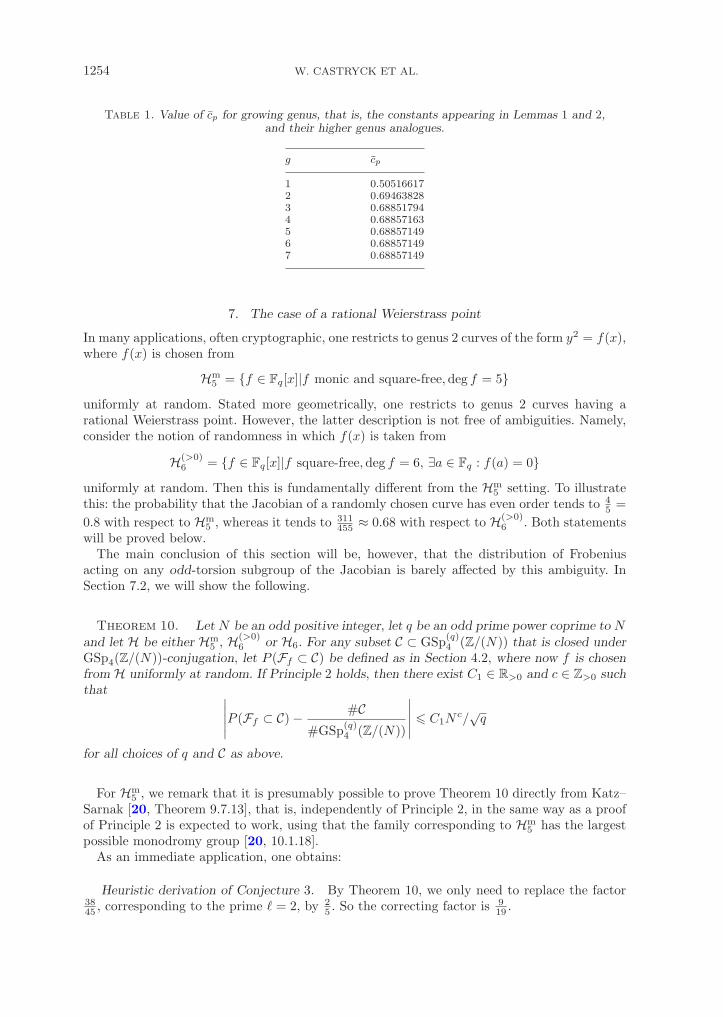
oscillates, but converges rapidly to its limiting value. This is illustrated numerically in Table 1.Of all genera, elliptic curves disfavor prime orders to the biggest extent, and the Jacobians ofgenus 2 curves disfavor prime orders to the least extent.
1254 W. CASTRYCK ET AL.
Table 1. Value of cp for growing genus, that is, the constants appearing in Lemmas 1 and 2,and their higher genus analogues.
g cp
1 0.505166172 0.694638283 0.688517944 0.688571635 0.688571496 0.688571497 0.68857149
7. The case of a rational Weierstrass point
In many applications, often cryptographic, one restricts to genus 2 curves of the form y2 = f(x),where f(x) is chosen from
Hm5 = {f ∈ Fq[x]|f monic and square-free,deg f = 5}
uniformly at random. Stated more geometrically, one restricts to genus 2 curves having arational Weierstrass point. However, the latter description is not free of ambiguities. Namely,consider the notion of randomness in which f(x) is taken from
H(>0)6 = {f ∈ Fq[x]|f square-free,deg f = 6, ∃a ∈ Fq : f(a) = 0}
uniformly at random. Then this is fundamentally different from the Hm5 setting. To illustrate
this: the probability that the Jacobian of a randomly chosen curve has even order tends to 45 =
0.8 with respect to Hm5 , whereas it tends to 311
455 ≈ 0.68 with respect to H(>0)6 . Both statements
will be proved below.The main conclusion of this section will be, however, that the distribution of Frobenius
acting on any odd-torsion subgroup of the Jacobian is barely affected by this ambiguity. InSection 7.2, we will show the following.
Theorem 10. Let N be an odd positive integer, let q be an odd prime power coprime to Nand let H be either Hm
5 , H(>0)6 or H6. For any subset C ⊂ GSp(q)
4 (Z/(N)) that is closed underGSp4(Z/(N))-conjugation, let P (Ff ⊂ C) be defined as in Section 4.2, where now f is chosenfrom H uniformly at random. If Principle 2 holds, then there exist C1 ∈ R>0 and c ∈ Z>0 suchthat ∣∣∣∣∣P (Ff ⊂ C)− #C
#GSp(q)4 (Z/(N))
∣∣∣∣∣ � C1Nc/√
q
for all choices of q and C as above.
For Hm5 , we remark that it is presumably possible to prove Theorem 10 directly from Katz–
Sarnak [20, Theorem 9.7.13], that is, independently of Principle 2, in the same way as a proofof Principle 2 is expected to work, using that the family corresponding to Hm
5 has the largestpossible monodromy group [20, 10.1.18].
As an immediate application, one obtains:
Heuristic derivation of Conjecture 3. By Theorem 10, we only need to replace the factor3845 , corresponding to the prime � = 2, by 2
5 . So the correcting factor is 919 .

THE PROBABILITY THAT A GENUS 2 JACOBIAN HAS PRIME ORDER 1255
7.1. Rational 2-torsion in genus 2
Some material in this section has appeared in the literature before, see, for example, [6,Section 2].
Lemma 4. Every non-trivial 2-torsion point on the Jacobian of a genus 2 curve over Fq
(thought of as a divisor class) contains a unique pair of divisors {Pi − Pj , Pj − Pi}, where Pi
and Pj are distinct Weierstrass points.
Proof. It is obvious that Pi − Pj and Pj − Pi are linearly equivalent and that they mapto a 2-torsion point on the Jacobian. By Riemann–Roch, this point is non-trivial and twodifferent pairs give rise to distinct 2-torsion points. Since there are 15 non-trivial 2-torsionpoints on the Jacobian of a genus 2 curve, and since there are 15 pairs in a set of 6 elements,the correspondence must be one to one.
We immediately obtain (compare with Theorem 9) the following.
Lemma 5. The Jacobian of a genus 2 curve over Fq defined by an equation of the formy2 = f(x) with f ∈ Hm
5 (resp. f ∈ H6) has a non-trivial rational 2-torsion point if and only iff is reducible (resp. f has a factor of degree 2).
Proof. By Lemma 4, there exists a non-trivial rational 2-torsion point if and only if thereare Weierstrass points P1 and P2 such that {P1, P2} is closed under qth power Frobenius.
This allows us to estimate the probability that the Jacobian has even order.
Lemma 6. Let fm5 ∈ Hm
5 , f(>0)6 ∈ H(>0)
6 and f6 ∈ H6 be chosen uniformly at random. Let
Cm5 , C
(>0)6 and C6 denote the corresponding genus 2 curves. Then as q →∞
(i) P (#Jac(Cm5 )(Fq) is even)→ 4
5 ;(ii) P (#Jac(C6)(Fq) is even)→ 26
45 ;(iii) P (#Jac(C(>0)
6 )(Fq) is even)→ 311455 .
Proof. We leave this as an exercise, or refer to Table 2.
We will now describe the symplectic structure of the 2-torsion subgroup in more detail. Fixa genus 2 curve C/Fq and let P1, . . . , P6 be its Weierstrass points. Following Lemma 4, everynon-trivial element of Jac(C)[2] can be identified with a unique pair of distinct points {Pi, Pj},and the group structure can be described by the rules⎧⎨
⎩{Pi, Pj}+ {Pi, Pj} = 0{Pi, Pj}+ {Pi, Pk} = {Pj , Pk} if j �= k{Pi, Pj}+ {Pk, P�} = {remaining two points} if {i, j} ∩ {k, �} = ∅.
The Weil pairing can be seen to satisfy
e2({Pi, Pj}, {Pk, P�}) = (−1)#{i,j,k,�}
for all i, j, k, � ∈ {1, . . . , 6}.We use this to prove the following.

1256 W. CASTRYCK ET AL.
Table 2. Factorization patterns of f(x) ∈ H6,Hm5 and the corresponding
Frobenius conjugacy classes.
H6 Hm5 Conjugacy classes of Sp4(F2)
Pattern Probability Pattern Probability Representant Size Order Fq-rank Trace
6 ≈1
6
(1 1 0 10 1 0 11 1 1 10 0 1 1
)120 6 0 0
5,1 ≈1
55 ≈1
5
(0 1 1 00 0 1 00 1 0 11 1 0 1
)144 5 0 1
4,2 ≈1
8
(0 1 0 01 0 0 00 0 0 11 0 1 0
)90 4 1 0
4,1,1 ≈1
84,1 ≈1
4
(1 0 1 11 0 0 10 1 0 11 1 1 1
)90 4 1 0
3,3 ≈ 1
18
(1 0 1 10 1 1 00 1 0 01 1 0 0
)40 3 0 0
3,2,1 ≈1
63,2 ≈1
6
(1 1 0 00 1 1 10 1 0 11 1 1 1
)120 6 1 1
3,1,1,1 ≈ 1
183,1,1 ≈1
6
(1 0 0 00 0 0 10 0 1 00 1 0 1
)40 3 2 1
2,2,2 ≈ 1
48
(0 0 0 11 0 1 00 1 0 11 0 0 0
)15 2 2 0
2,2,1,1 ≈ 1
162,2,1 ≈1
8
(0 0 1 00 1 0 01 0 0 00 1 0 1
)45 2 2 0
2,1,1,1,1 ≈ 1
482,1,1,1 ≈ 1
12
(0 1 1 00 1 0 01 1 0 01 1 1 1
)15 2 3 0
1,1,1,1,1,1 ≈ 1
7201,1,1,1,1 ≈ 1
120
(1 0 0 00 1 0 00 0 1 00 0 0 1
)1 1 4 0
For instance, the pattern 3, 1, 1, 1 means that f(x) ∈ H6 factors into three linear polynomials and oneirreducible cubic polynomial. The probability of this event is approximately 1
3· 1
3!11
= 118
. Thecorresponding conjugacy class of Frobenius is generated by the depicted matrix and contains 40 elements.Every such element has order 3 and trace 1, and its eigenspace for eigenvalue 1 is two-dimensional(that is, dim Jac(C)[2](Fq) = 2).
Theorem 11. Let q be an odd prime power. There exist W0, . . . ,W6 ⊂ Sp4(F2) such thatfor any curve C/Fq of genus 2, any symplectic basis of Jac(C)[2], and any r ∈ {0, . . . , 6}, thematrix F of qth power Frobenius with respect to this basis satisfies
F ∈ Wr if and only if C has r rational Weierstrass points.
The cardinalities of the Wr are 265, 264, 135, 40, 15, 0 and 1, respectively.
Proof. There exist six subsets U ⊂ Jac(C)[2] that are maximal with respect to the conditionthat u1, u2 ∈ U and u1 �= u2 implies e2(u1, u2) = −1, namely
Ui = {{Pi, Pj}|j ∈ {1, 2, . . . , 6} \ {i}} for i = 1, . . . , 6.
Since N = 2, the choice of a primitive Nth root of unity is canonical, hence the Weil pairingdefines unambiguously a symplectic pairing on Jac(C)[2]. After having fixed a symplectic basis,every symplectic matrix induces a permutation of {U1, . . . , U6}. In fact, this induces a groupisomorphism Sp4(F2)→ Sym(6). Indeed, it is easy to see that the above induces an injectivegroup homomorphism, and surjectivity follows from #Sp4(F2) = #Sym(6) = 720. Then thesets Wr are the pre-images under this isomorphism of the set of permutations having exactly
THE PROBABILITY THAT A GENUS 2 JACOBIAN HAS PRIME ORDER 1257
r fixed points. While the isomorphism depends on the choice of symplectic basis, the sets Wr
do not, because they are invariant under conjugation.
Pushing the argument a little further, one actually sees that the conjugacy class of Frobenius,which under the above group isomorphism corresponds to a conjugacy class of Sym(6), iscompletely determined by the factorization pattern of f(x), and conversely. Note that thereare 11 conjugacy classes in Sym(6) ∼= Sp4(F2) and that there are 11 ways to partition thenumber 6. Since the probability of having a certain factorization pattern is easily estimatedusing the well-known fact that a polynomial of degree d is irreducible with probability about1/d, this unveils the complete stochastic picture of Jac(C)[2], as shown in Table 2.
Corollary 2. Principle 2 holds for g = N = 2.
Proof. This can be read off from Table 2. The only additional concern is the bound on theerror term, but this is easily verified.
7.2. Equidistribution in odd level
In this section, we will prove Theorem 10. Consider f ∈ H(>0)6 , so that y2 = f(x) defines a
genus 2 curve having a rational Weierstrass point (a, 0). Then the birational change of variables
x←− 1x
+ a and y ←− y
x3,
transforms this into y2 = f ′(x) with f ′ ∈ H5. This leads us to defining a relation
ρ ⊂ H(>0)6 ×H5
associating to f ∈ H(>0)6 all polynomials of H5, that can be obtained through the above
procedure. However, this correspondence is not uniform, because of the number of choicesthat can be made for a, that is, the number of rational roots of f . This is the reason why thenotions of randomness with respect to H5 (or Hm
5 ) and H(>0)6 are fundamentally different, as
reflected in Lemma 6.We are led to introducing the following notation. For r ∈ {0, . . . , 6}, define
H(r)6 = {f ∈ Fq[x]|f square-free,deg f = 6, f has precisely r rational zeroes}
so that
H6 =6⊔
r=0
H(r)6 and H(>0)
6 =6⊔
r=1
H(r)6 . (14)
Similarly, for r ∈ {0, . . . , 5} we introduce
H(r)5 = {f ∈ Fq[x]|f square-free of degree 5, f has precisely r rational zeroes},
so that
H5 =5⊔
r=0
H(r)5 .
Note that H(5)6 and H(4)
5 are empty. We implicitly omit these sets to avoid probabilities of thetype 0
0 . Similarly, we assume that q > 6 so that none of the other sets is empty.Now because of (14), to prove Theorem 10 for H(>0)
6 , it suffices to do so for each H(r)6
(r = 1, . . . , 6). Similarly, by the discussion in Section 2, we can use H5 instead of Hm5 , and it
1258 W. CASTRYCK ET AL.
is sufficient to prove Theorem 10 for H(r)5 (r = 0, . . . , 5) in this case. Finally, by Lemma 7, the
cases H(r)5 can in turn be reduced to the cases H(r)
6 .
Lemma 7. Let S0 = {f ∈ H5|f(0) �= 0}. For each r = 1, . . . , 6, the restriction of ρ to
H(r)6 × (H(r−1)
5 ∩ S0)
is uniform.
Proof. This is immediate.
We are now ready to prove Theorem 10.
Proof of Theorem 10. By the above discussion, it suffices to estimate the conditionalprobabilities
P (Ff ⊂ C|f ∈ H(r)6 ) =
P (Ff ⊂ C and f ∈ H(r)6 )
P (f ∈ H(r)6 )
for r = 1, . . . , 6. By Theorem 11, f ∈ H(r)6 is equivalent to saying that the conjugacy class
of Frobenius, acting on the 2-torsion points of the Jacobian of y2 = f(x), is contained in Wr.Denote this conjugacy class by Ff,2. Similarly, let Ff,2N denote the conjugacy class of Frobeniusacting on the 2N -torsion points.
Since N is odd, we have a canonical isomorphism
GSp(q)4 (Z/(2N)) ∼= GSp(q)
4 (F2)⊕GSp(q)4 (Z/(N)),
allowing us to consider Wr ⊕ C as a subset of GSp(q)4 (Z/(2N)). Because it is the union of a
number of orbits under GSp4(Z/(2N))-conjugation, there exist C1 ∈ R>0 and c ∈ Z>0, suchthat ∣∣∣∣∣P (Ff,2N ⊂ Wr ⊕ C)− #(Wr ⊕ C)
#GSp(q)4 (Z/(2N))
∣∣∣∣∣ � C1Nc/√
q (15)
for all choices of q, N and C. In particular, for N = 1, this gives∣∣∣∣∣P (f ∈ H(r)6 )− #Wr
#GSp(q)4 (F2)
∣∣∣∣∣ � C1/√
q. (16)
Since
P (Ff,2N ⊂ Wr ⊕ C) = P (Ff ⊂ C and Ff,2 ⊂ Wr) = P (Ff ⊂ C and f ∈ H(r)6 )
and#(Wr ⊕ C)
#GSp(q)4 (Z/(2N))
=#Wr
#GSp(q)4 (F2)
· #C#GSp(q)
4 (Z/(N)),
inequality (15) can be rewritten as∣∣∣∣∣P (Ff ⊂ C|f ∈ H(r)6 )− #Wr/#GSp(q)
4 (F2)
P (f ∈ H(r)6 )
· #C#GSp(q)
4 (Z/(N))
∣∣∣∣∣ � C1Nc/√
q
P (f ∈ H(r)6 )
.
It follows from (16) that there is a C2 ∈ R+ such that∣∣∣∣∣P (Ff ⊂ C|f ∈ H(r)6 )− #C
#GSp(q)4 (Z/(N))
∣∣∣∣∣ � C2Nc/√
q
for all choices of q, N and C. This completes the proof.
THE PROBABILITY THAT A GENUS 2 JACOBIAN HAS PRIME ORDER 1259
8. The number of points on the curve itself
Up to now we have focused entirely on the number of rational points on the Jacobian of acurve. However, the random matrix framework allows us to consider the number of rationalpoints on the curve itself as well.
For any pair of distinct primes p > 2 and �, and any t ∈ F�, we define the following constants:
a�,t,p := #{(x, y) ∈ F×� × (F×
� \{−p})|(x + y/x)(1 + p/y) = t},
A�,t,p := �4((�− 1)(�− 2) + a�,t,p) +
{�6 − �4 if t = 0,0 otherwise,
B� := �4(�2 − 1)2,
C�,t := �5(�− 1)(�3 − �− 1) +
{�7 − �6 if t = 0,0 otherwise.
Note that, in general, it is impossible to find a closed formula for a�,t,p since it typically describesthe number of points on an elliptic curve over F� (though it is clear that a�,t,p lies close to �).Let P (p, �, t) be the probability that the number of rational points on the non-singular completemodel of the curve C : y2 = f(x), with f(x) chosen uniformly at random from H6, is congruentto p + 1− t modulo �.
Theorem 12. There exist C1 ∈ R>0 and c ∈ Z>0, such that∣∣∣∣∣P (p, �, t)− A�,t,p + B� + C�,t
�4 · (�4 − 1) · (�2 − 1)
∣∣∣∣∣ � C1�c/√
p
for all p, �, t as above.
Proof. Because the trace of a matrix is invariant under conjugation, it suffices by Principle 2(proved for � odd by Achter [2, Theorem 3.1], and for � = 2 in Corollary 2) to count the numberof matrices M in GSp(p)
4 (F�) with trace t, and show that it equals A�,t,p + B� + C�,t. Our maintool is the following Bruhat decomposition of Sp4(F�), proved by Kim [22]. Consider the group
P ={(
A AB0 tA−1
)∣∣∣∣ A,B ∈ F2×2� , A invertible, B symmetric
}, (17)
then we have the disjoint union
Sp4(F�) = P � Pσ1P � Pσ2P ,
where
σ1 =
⎛⎜⎜⎝
0 0 1 00 1 0 0−1 0 0 00 0 0 1
⎞⎟⎟⎠ and σ2 = Ω =
(0 I2−I2 0
).
For r ∈ {1, 2}, consider the subgroup
Ar = {M ∈ P |σrMσ−1r ∈ P}.
Then one can find unique representatives for the elements of PσrP by rewriting
PσrP = Pσr(Ar\P ),
where Ar\P should be seen as a set of representatives of the right cosets of Ar in P . Thisimplies that
|PσrP | = |P | · |Ar\P |.
1260 W. CASTRYCK ET AL.
One can prove (see [22]) that |A1\P | = �2 + � and |A2\P | = �3. Taking σ0 = I4, the Bruhatdecomposition of Sp4(F�) implies the following partition of GSp(p)
4 (F�):
GSp(p)4 (F�) =
2⊔r=0
dpPσrP.
We will do a component-wise count of the number of matrices having trace t. First we observethat
|{M ∈ dpPσrP |Tr(M) = t}| = |Ar\P | · |{M ∈ dpPσr|Tr(M) = t}|for r = 1, 2. Indeed, every element of dpPσrP has a unique representation of the form
dpMσrN
with M ∈ P and N ∈ Ar\P (where Ar\P is thought of as a set of representatives of the rightcosets of Ar). Using this representation, the map
dpPσrP −→ dpPσr : dpMσrN �−→ dp(d−1p NdpM)σr
is surjective and |Ar\P |-to-1. Since dpMσrN and dp(d−1p NdpM)σr are conjugated, the
observation follows.A matrix M ∈ dpP can be written as
(A AB0 p·tA−1
)with A ∈ GL2(F�) and B ∈ F2×2
�
symmetric.First, we consider Mσ1, whose trace equals −(AB)1,1 + A2,2 + (p · tA−1)2,2, where the index
notation refers to the corresponding entries. Fix A and let B vary. Then because (AB)1,1 =A1,1B1,1 + A1,2B2,1 and not both A1,1 and A1,2 can be zero, we find that each trace occursequally often. We conclude that traces are uniformly distributed in dpPσ1. Next, for Mσ2 wefind that Tr(Mσ2) = −Tr(AB), which is uniformly distributed for all A not of the form
(0 a−a 0
),
and which is zero if A does have this form. Using the above formulas for |Ar\P | and using|GL2(F�)| = �(�2 − 1)(�− 1), we find that the number of matrices in dpPσ1 � dpPσ2 havingtrace t equals B� + C�,t.
Finally, we consider M ∈ dpP when Tr(M) = Tr(A) + Tr(pA−1). We write A =(
a bc d
)and let
δ = ad− bc be its determinant. Clearly Tr(M) = Tr(A) · (1 + p/δ). There are �(�2 − 1) matricesA with determinant −p, in which case this trace equals 0. So suppose that δ �= −p. When a = 0it is easy to see that we have uniform distribution, so we also suppose that a �= 0. We can replaced by (δ + bc)/a and again, if b �= 0 we will find uniformity. Finally the case b = 0 gives as trace
(a + δ/a)(1 + p/δ),
so that an easy calculation shows that the number of matrices in dpP with trace tequals A�,t,p.
Table 3 gives the respective probabilities for various small �. Note that the probabilities ofC and Jac(C) having an even number of rational points are the same, despite the fact thatthese events do not coincide. Also note from Table 3 that trace 0 is favored. This is a generalphenomenon that can be seen as follows. It is not hard to verify that if 2t(t2 − 16p) ≡ 0 mod �,the curve (x + y/x)(1 + p/y) = t in the definition of a�,t,p is reducible or has genus 0, in whichcase a�,t,p can be explicitly computed. It is equal to zero if � = 2. For t ≡ 0 mod � and � > 2we can compute the following estimate for P (p, �, t):
�9 − �6 − �5 − �4
�4(�4 − 1)(�2 − 1)=
�3 − �− 1(�2 − 1)2
if p is a square modulo � and
�9 − �6 − �5 + �4
�4(�4 − 1)(�2 − 1)=
�3 + �− 1�4 − 1
THE PROBABILITY THAT A GENUS 2 JACOBIAN HAS PRIME ORDER 1261
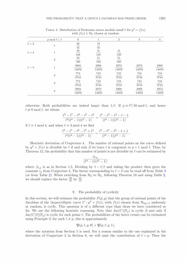
Table 3. Distribution of Frobenius traces modulo small � for y2 = f(x),with f(x) ∈ H6 chosen at random.
p mod � \ t 0 1 2 3 4
� = 21
26
45
19
45
� = 3 146
128
41
128
41
128
258
160
51
160
51
160
� = 5 13094
14976
2969
14976
2972
14976
2972
14976
2969
14976
2774
3744
743
3744
742
3744
742
3744
743
3744
3774
3744
742
3744
743
3744
743
3744
742
3744
43094
14976
2972
14976
2969
14976
2969
14976
2972
14976
otherwise. Both probabilities are indeed larger than 1/�. If p ≡ t2/16 mod �, and hencet �≡ 0 mod �, we obtain
�9 − �7 − �6 − �5 − �4
�4(�4 − 1)(�2 − 1)=
�5 − �3 − �2 − �− 1(�4 − 1)(�2 − 1)
if � ≡ 1 mod 4, and when � ≡ 3 mod 4 we find
�9 − �7 − �6 − �5 + �4
�4(�4 − 1)(�2 − 1)=
�5 − �3 − �2 − � + 1(�4 − 1)(�2 − 1)
.
Heuristic derivation of Conjecture 4. The number of rational points on the curve definedby y2 = f(x) is divisible by � if and only if its trace t is congruent to p + 1 mod �. Thus, byTheorem 12, the probability that this number of points is not divisible by � can be estimated by
β�,p
(�4 − 1)(�2 − 1),
where β�,p is as in Section 1.5. Dividing by 1− 1/� and taking the product then gives theconstant cp from Conjecture 4. The factor corresponding to � = 2 can be read off from Table 3(or from Table 2). When switching from H6 to H5, following Theorem 10 and using Table 2,we should replace the factor 38
45 by 1615 .
9. The probability of cyclicity
In this section, we will estimate the probability P (p, g) that the group of rational points of theJacobian of the (hyper)elliptic curve C : y2 = f(x), with f(x) chosen from H2g+2 uniformlyat random, is cyclic. This question is of a different type than those we have considered sofar. We use the following heuristic reasoning. Note that Jac(C)(Fp) is cyclic if and only ifJac(C)[�](Fp) is cyclic for each prime �. The probabilities of the latter events can be estimatedusing Principle 2: for each � �= p, this is approximately
P(p, �, g, 0) + P(p, �, g, 1),
where the notation from Section 5 is used. For a reason similar to the one explained in thederivation of Conjecture 2 in Section 6, we will omit the contribution of � = p. Then the
1262 W. CASTRYCK ET AL.
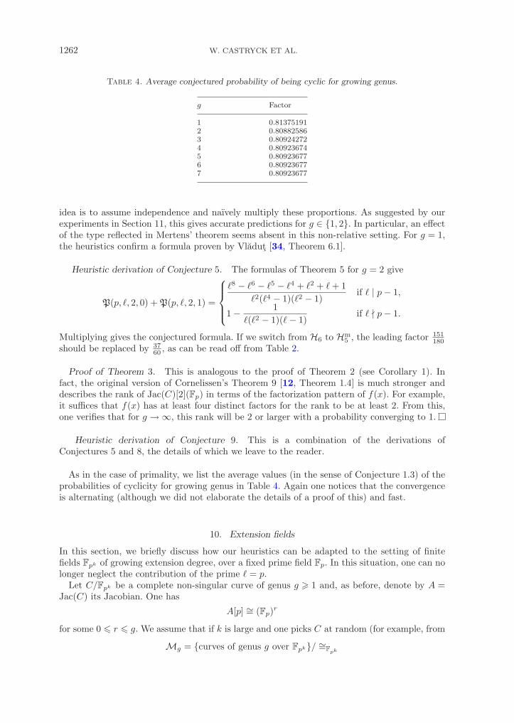
Table 4. Average conjectured probability of being cyclic for growing genus.
g Factor
1 0.813751912 0.808825863 0.809242724 0.809236745 0.809236776 0.809236777 0.80923677
idea is to assume independence and naıvely multiply these proportions. As suggested by ourexperiments in Section 11, this gives accurate predictions for g ∈ {1, 2}. In particular, an effectof the type reflected in Mertens’ theorem seems absent in this non-relative setting. For g = 1,the heuristics confirm a formula proven by Vladut [34, Theorem 6.1].
Heuristic derivation of Conjecture 5. The formulas of Theorem 5 for g = 2 give
P(p, �, 2, 0) + P(p, �, 2, 1) =
⎧⎪⎪⎨⎪⎪⎩
�8 − �6 − �5 − �4 + �2 + � + 1�2(�4 − 1)(�2 − 1)
if � | p− 1,
1− 1�(�2 − 1)(�− 1)
if � � p− 1.
Multiplying gives the conjectured formula. If we switch from H6 to Hm5 , the leading factor 151
180should be replaced by 37
60 , as can be read off from Table 2.
Proof of Theorem 3. This is analogous to the proof of Theorem 2 (see Corollary 1). Infact, the original version of Cornelissen’s Theorem 9 [12, Theorem 1.4] is much stronger anddescribes the rank of Jac(C)[2](Fp) in terms of the factorization pattern of f(x). For example,it suffices that f(x) has at least four distinct factors for the rank to be at least 2. From this,one verifies that for g →∞, this rank will be 2 or larger with a probability converging to 1.
Heuristic derivation of Conjecture 9. This is a combination of the derivations ofConjectures 5 and 8, the details of which we leave to the reader.
As in the case of primality, we list the average values (in the sense of Conjecture 1.3) of theprobabilities of cyclicity for growing genus in Table 4. Again one notices that the convergenceis alternating (although we did not elaborate the details of a proof of this) and fast.
10. Extension fields
In this section, we briefly discuss how our heuristics can be adapted to the setting of finitefields Fpk of growing extension degree, over a fixed prime field Fp. In this situation, one can nolonger neglect the contribution of the prime � = p.
Let C/Fpk be a complete non-singular curve of genus g � 1 and, as before, denote by A =Jac(C) its Jacobian. One has
A[p] ∼= (Fp)r
for some 0 � r � g. We assume that if k is large and one picks C at random (for example, from
Mg = {curves of genus g over Fpk}/ ∼=Fpk
THE PROBABILITY THAT A GENUS 2 JACOBIAN HAS PRIME ORDER 1263
uniformly at random), one has r = g with probability ≈ 1. This is reasonable, because themoduli space Ag of abelian varieties of dimension g is stratified by rank, the stratumcorresponding to r = g having the biggest dimension [28, Theorem 4.1]. We do not claima proof of this assumption however, although for hyperelliptic curves this is a known fact[4, 29]. If r = g, then the matrix of the pkth power Frobenius acting on A[p] with respect toany Fp-basis is an element of GLg(Fp). Thus, in that case, we can unambiguously associate toC a conjugacy class of matrices of pkth power Frobenius, denoted by FC . The expectation isthat for every union of conjugacy classes C ⊂ GLg(Fp), the probability that FC ⊂ C becomesproportional to #C (as k →∞).
Returning to hyperelliptic curves, let P (Ff,h ⊂ C) be the probability that the conjugacy classof Frobenius associated to the hyperelliptic curve y2 + h(x)y = f(x), where (f, h) is chosen fromHg+1,2g+2 uniformly at random, is contained in C. As explained in Section 2, for p > 2, onecan assume h(x) = 0 and f(x) chosen from H2g+2 if desired.
Principle 3. Let g ∈ {1, 2}. There exist C1 ∈ R>0 and c ∈ Z>0 such that∣∣∣∣P (Ff,h ⊂ C)− #C#GLg(Fp)
∣∣∣∣ � C1pc/√
pk
for all choices of p, k and C as above.
The assumption g ∈ {1, 2} is a ‘safety’ measure, because we do not feel comfortable withthe behavior of the hyperelliptic locus inside Ag as soon as g > 2. In fact, even for g = 2some prudence is needed with respect to Principle 3: the literature seems to contain much lessevidence in its favor than in the cases of Principles 1 and 2.
In contrast, for g = 1, Principle 3 can be proved by applying the Hasse–Weil bound to theIgusa curve Ig(p), whose Fpk -rational points essentially parameterize pairs (E,P ), where E/Fpk
is an elliptic curve and P ∈ E[p](Fpk). A more elementary but longer proof is given below. Weinclude it because we believe some intermediate statements are interesting in their own right(in fact, we develop a version of [32, Theorem V.4.1], which is on the Legendre family, forWeierstrass equations). First note that Principle 3 is trivial for p = 2 and for p = 3; in thelatter case because quadratic twisting provides a bijection between the set of elliptic curveshaving trace 1 mod 3 and the set of elliptic curves with trace 2 mod 3.
Theorem 13. Let p � 5 be a prime number, let k � 1 be an integer and let t ∈ {1, . . . ,p− 1}. Let St be the set of couples in
S = HA,B = {(A,B) ∈ (Fpk)2|4A3 + 27B2 �= 0}for which the trace T of the pkth power Frobenius of the elliptic curve given by y2 = x3 +Ax + B satisfies T ≡ t mod p. Then #S = p2k − pk and∣∣∣∣#St − #S
p− 1
∣∣∣∣ � 3p3k/2+1.
Proof. We leave it as an exercise to show that #S = p2k − pk.For each (A,B) ∈ S, one has that T mod p equals the norm (with respect to Fpk/Fp) of the
coefficient cA,B of xp−1 in
(x3 + Ax + B)(p−1)/2
(see the proof of [32, Theorem V.4.1(a)]). Lemma 8 shows that for every γ ∈ F×pk , the
polynomial cA,B − γ is absolutely irreducible when A and B are considered to be variables.

1264 W. CASTRYCK ET AL.
Now write S′t for the set of couples (A,B) ∈ (Fpk)2 in which cA,B evaluates to an element
γ ∈ Fpk \ {0} with norm t (regardless of the condition 4A3 + 27B2 �= 0). There are
pk − 1p− 1
such γ elements. For each of these, the polynomial cA,B − γ defines a plane affine curve, by theclaimed irreducibility. Its degree is bounded by d = 3(p− 1)/2, hence its (geometric) genus isat most (d− 1)(d− 2)/2, and the number of points at infinity is at most d. Therefore, the setS′
γ ⊂ S′t of couples satisfying cA,B = γ is subject to
|#S′γ − (pk + 1)| � (d− 1)(d− 2)
√pk + d � 9
4pk/2+2
by the Hasse–Weil bound. Note that cA,B = γ defines an affine, possibly singular curve, so somecaution is needed when applying the Hasse–Weil bound (see [13, Theorem 5.4.1] for details).
Summing up, and using (pk − 1)/(p− 1) � 54pk−1 (since p � 5),∣∣∣∣#S′
t −p2k − 1p− 1
∣∣∣∣ � 4516
p3k/2+1.
Because #(S′t \ St) � pk and 5pk−1 � pk � 1
11p(3/2)k+1, we obtain∣∣∣∣#St − p2k − pk
p− 1
∣∣∣∣ �∣∣∣∣#St − p2k − 1
p− 1
∣∣∣∣+ pk − 1p− 1
�(
4516
+111
+54· 155
)p(3k/2)+1,
which completes the proof.
Lemma 8. Let p � 5 be a prime number and let cA,B ∈ Fp[A,B] be the coefficient of xp−1
in
(x3 + Ax + B)(p−1)/2 ∈ Fp[A,B][x].
Then cA,B is homogeneous of (2, 3)-weighted degree (p− 1)/2, non-zero and absolutely square-free. As a consequence, for any γ ∈ F×
p , the polynomial
cA,B − γ ∈ Fp[A,B]
is irreducible.
Proof. One verifies that
cA,B =�(p−1)/4�∑
i=(p−1)/6
(p− 1
2i
)(i
3i− p− 12
)A3i−(p−1)/2B(p−1)/2−2i, (18)
from which it immediately follows that cA,B is non-zero and homogeneous of degree (p− 1)/2if we equip A and B with weights 2 and 3, respectively. It is easy to verify that A and B appearas a factor at most once.
Let c′A,B be obtained from cA,B by deleting the factors A and B when possible. Define εA
and εB to be 1 if a factor A and B was deleted, respectively, and 0 otherwise. Then c′A,B isstill homogeneous, of degree (p− 1)/2− 2εA − 3εB . After dividing by a suitable power of Aand considering the resulting polynomial in the single variable B2/A3, one verifies that c′A,B
splits (over Fp) asc(B2 − a1A
3)(B2 − a2A3) . . . (B2 − arA
3), (19)
with r = 16 ((p− 1)/2− 2εA − 3εB) and all c, ai �= 0. Each of these factors corresponds to a
ji �= 0, 1728 for which the elliptic curve over Fp with j-invariant ji is supersingular, and

THE PROBABILITY THAT A GENUS 2 JACOBIAN HAS PRIME ORDER 1265
conversely, all supersingular j-invariants different from 0 and 1728 must be represented thisway. Now the number of supersingular j-invariants different from 0 and 1728 is precisely givenby r (see the proof of [32, Theorem V.4.1(c)]). Therefore, all factors in (19) must be different,and in particular cA,B must be square-free.
Now let γ ∈ F×p and suppose we had a non-trivial factorization
cA,B − γ = (F1 + X1)(F2 + X2),
where F1 and F2 are the components of highest (weighted) degree of the respective factors.Then it follows that F1F2 = cA,B , so F1 and F2 cannot have a common factor. It also followsthat
X1F2 + X2F1 + X1X2 + γ = 0. (20)
Let X ′1 and X ′
2 be the components of highest degree of X1 and X2, respectively. Supposedeg X1F2 > deg X2F1. Then X ′
1F2 is zero, because it cannot be cancelled in (20). But then X ′1 =
X1 = 0 and we run into a contradiction. By symmetry, we conclude that deg X1F2 = deg X2F1.But then X ′
1F2 + X ′2F1 = 0. So all factors of F1 must divide X ′
1F2, which is impossible unlessX ′
1 = 0, and we again run into a contradiction.
Table 5. �-torsion frequencies and cp values for C(Fp) using random elliptic curvesC : y2 = f(x) with f ∈ Hm
3 .
p � = 2 � = 3 � = 5 � = 7 cp
1012 + 39 Observed 0.6654 0.3749 0.2507 0.1664 0.5492Predicted 0.6667 0.3750 0.2500 0.1667 0.5564
1012 + 61 Observed 0.6662 0.5003 0.2083 0.1664 0.4686Predicted 0.6667 0.5000 0.2083 0.1667 0.4646
1012 + 63 Observed 0.6672 0.3756 0.2503 0.1460 0.5600Predicted 0.6667 0.3750 0.2500 0.1458 0.5642
1012 + 91 Observed 0.6660 0.4989 0.2089 0.1454 0.4818Predicted 0.6667 0.5000 0.2083 0.1458 0.4794
[1012, 1012 + 4 × 10⁶] Observed 0.6666 0.4374 0.2396 0.1631 0.5044Predicted 0.6667 0.4375 0.2396 0.1632 0.5052
Sample size is 106 (or 102 for p ranging over the interval [1012, 1012 + 4 × 10⁶]).
Table 6. �-torsion frequencies and cp values for Jac(C)(Fp) using random genus 2 curvesC : y2 = f(x) with f ∈ Hm
5 .
p � = 2 � = 3 � = 5 � = 7 cp
106 + 3 Observed 0.7991 0.3616 0.2395 0.1628 0.3426Predicted 0.8000 0.3609 0.2396 0.1632 0.3444
106 + 37 Observed 0.8000 0.4376 0.2393 0.1626 0.3056Predicted 0.8000 0.4375 0.2396 0.1632 0.3037
106 + 81 Observed 0.8001 0.3619 0.2066 0.1632 0.3571Predicted 0.8000 0.3609 0.2067 0.1632 0.3593
106 + 121 Observed 0.8003 0.4376 0.2059 0.1637 0.3197Predicted 0.8000 0.4375 0.2067 0.1632 0.3189
[106, 2 × 10⁶] Observed 0.8000 0.3992 0.2314 0.1604 0.3285Predicted 0.8000 0.3992 0.2314 0.1602 0.3290
Sample size is 106 (or 102 for p ranging over the interval [106, 2 × 10⁶]).

1266 W. CASTRYCK ET AL.
We conclude this section with a derivation of Conjectures 6 and 7. To apply our heuristics,we need to generalize the material from Section 6. In analogy with the notation employedthere, for any prime power q, any prime number � and any integer g � 1, let P (q, �, g) be theprobability that the Jacobian of the hyperelliptic curve y2 + h(x)y = f(x), with (f, h) chosenfrom Hg+1,2g+2 uniformly at random, has an Fq-rational �-torsion point. Let Q(q, �, g) be theproportion of matrices of GSp(q)
2g (F�) having 1 as an eigenvalue if � � q, and the proportion ofmatrices of GLg(F�) if � | q. Then according to Principles 2 and 3, if g ∈ {1, 2}, we have thatP (q, �, g)→ Q(q, �, g) as q →∞. Recall from Theorem 6 that one has
Q(q, �, g) =
⎧⎪⎪⎪⎪⎨⎪⎪⎪⎪⎩−
g∑r=1
�rr∏
j=1
(1− �2j)−1 if � | q − 1,
−g∑
r=1
r∏j=1
(1− �j)−1 if � � q − 1(21)
Table 7. cp values for the number of points on random genus 2 curves y2 = f(x) with f ∈ Hm5 .
109 + 7 109 + 9 109 + 21 109 + 33
Observed 1.0162 1.0738 1.0892 1.0945Predicted 1.0194 1.0790 1.0865 1.0898
Sample size is 106. The deviations are larger here due to the shorter intervals (of width approximately8 × 109/2 versus 8 × 10⁶ and 4 × 10⁶ in Tables 5 and 6).
Table 8. Trace distributions modulo � for random genus 2 curves y2 = f(x) with f ∈ Hm5 .
p � t ≡ 0 t ≡ 1 t ≡ 2 t ≡ 3 t ≡ 4
106 + 3 2 Observed 0.4658 0.5342Predicted 0.4667 0.5333
3 Observed 0.3598 0.3205 0.3197Predicted 0.3594 0.3203 0.3203
5 Observed 0.2072 0.1988 0.1978 0.1981 0.1981Predicted 0.2067 0.1982 0.1985 0.1985 0.1982
106 + 37 2 Observed 0.4653 0.5346Predicted 0.4667 0.5333
3 Observed 0.3628 0.3185 0.3186Predicted 0.3625 0.3188 0.3188
5 Observed 0.2070 0.1982 0.1981 0.1983 0.1984Predicted 0.2067 0.1985 0.1982 0.1982 0.1985
106 + 39 2 Observed 0.4667 0.5332Predicted 0.4667 0.5333
3 Observed 0.3593 0.3206 0.3202Predicted 0.3594 0.3203 0.3203
5 Observed 0.2068 0.1978 0.1983 0.1989 0.1982Predicted 0.2066 0.1985 0.1983 0.1983 0.1985
[106, 2 × 10⁶] 2 Observed 0.4669 0.5331Predicted 0.4667 0.5333
3 Observed 0.3609 0.3194 0.3197Predicted 0.3625 0.3203 0.3203
5 Observed 0.2068 0.1982 0.1984 0.1981 0.1985Predicted 0.2067 0.1984 0.1984 0.1985 0.1984
Sample size is 106 (or 102 for p ranging over the interval [106, 2 × 10⁶]).
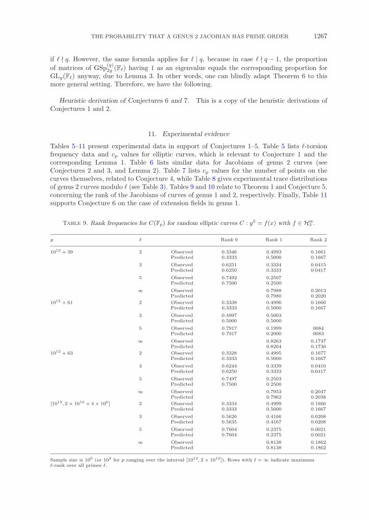
THE PROBABILITY THAT A GENUS 2 JACOBIAN HAS PRIME ORDER 1267
if � � q. However, the same formula applies for � | q, because in case � � q − 1, the proportionof matrices of GSp(q)
2g (F�) having 1 as an eigenvalue equals the corresponding proportion forGLg(F�) anyway, due to Lemma 3. In other words, one can blindly adapt Theorem 6 to thismore general setting. Therefore, we have the following.
Heuristic derivation of Conjectures 6 and 7. This is a copy of the heuristic derivations ofConjectures 1 and 2.
11. Experimental evidence
Tables 5–11 present experimental data in support of Conjectures 1–5. Table 5 lists �-torsionfrequency data and cp values for elliptic curves, which is relevant to Conjecture 1 and thecorresponding Lemma 1. Table 6 lists similar data for Jacobians of genus 2 curves (seeConjectures 2 and 3, and Lemma 2). Table 7 lists cp values for the number of points on thecurves themselves, related to Conjecture 4, while Table 8 gives experimental trace distributionsof genus 2 curves modulo � (see Table 3). Tables 9 and 10 relate to Theorem 1 and Conjecture 5,concerning the rank of the Jacobians of curves of genus 1 and 2, respectively. Finally, Table 11supports Conjecture 6 on the case of extension fields in genus 1.
Table 9. Rank frequencies for C(Fp) for random elliptic curves C : y2 = f(x) with f ∈ Hm3 .
p � Rank 0 Rank 1 Rank 2
1012 + 39 2 Observed 0.3346 0.4993 0.1661Predicted 0.3333 0.5000 0.1667
3 Observed 0.6251 0.3334 0.0415Predicted 0.6250 0.3333 0.0417
5 Observed 0.7492 0.2507Predicted 0.7500 0.2500
∞ Observed 0.7988 0.2013Predicted 0.7980 0.2020
1012 + 61 2 Observed 0.3338 0.4996 0.1666Predicted 0.3333 0.5000 0.1667
3 Observed 0.4997 0.5003Predicted 0.5000 0.5000
5 Observed 0.7917 0.1999 0084Predicted 0.7917 0.2000 0083
∞ Observed 0.8263 0.1737Predicted 0.8264 0.1736
1012 + 63 2 Observed 0.3328 0.4995 0.1677Predicted 0.3333 0.5000 0.1667
3 Observed 0.6244 0.3339 0.0416Predicted 0.6250 0.3333 0.0417
5 Observed 0.7497 0.2503Predicted 0.7500 0.2500
∞ Observed 0.7953 0.2047Predicted 0.7962 0.2038
[1012, 2 × 10¹² + 4 × 10⁶] 2 Observed 0.3334 0.4999 0.1666Predicted 0.3333 0.5000 0.1667
3 Observed 0.5626 0.4166 0.0208Predicted 0.5635 0.4167 0.0208
5 Observed 0.7604 0.2375 0.0021Predicted 0.7604 0.2375 0.0021
∞ Observed 0.8138 0.1862Predicted 0.8138 0.1862
Sample size is 106 (or 102 for p ranging over the interval [1012, 2 × 10¹²]). Rows with � = ∞ indicate maximum�-rank over all primes �.

1268 W. CASTRYCK ET AL.
The data in Tables 5–10 were obtained using the smalljac library [33], based on thealgorithms described in [21]. Table 11 was obtained using the intrinsic Magma [7] pointcounting function. We conducted our tests by sampling random curves C over finite fields Fp.We collected data both using fixed primes p, and for all primes in a given interval. For genus 1,
Table 10. Rank frequencies for Jac(C)(Fp) for random genus 2 curvesC : y2 = f(x) with f ∈ Hm
5 .
p � Rank 0 Rank 1 Rank 2 Rank 3 Rank 4
106 + 3 2 Observed 0.200113 0.416313 0.291528 0.083775 0.008271Predicted 0.200000 0.416667 0.291667 0.083333 0.008333
3 Observed 0.637964 0.320212 0.040254 0.001548 0.000022Predicted 0.639063 0.319444 0.039931 0.001543 0.000019
5 Observed 0.761095 0.236804 0.002101Predicted 0.760417 0.237500 0.002083
∞ Observed 0.589030 0.317489 0.085188 0.008293Predicted 0.589471 0.317443 0.084733 0.008352
106 + 81 2 Observed 0.200794 0.416446 0.290857 0.083593 0.008310Predicted 0.200000 0.416667 0.291667 0.083333 0.008333
3 Observed 0.637636 0.320698 0.040107 0.001533 0.000026Predicted 0.639063 0.319444 0.039931 0.001543 0.000019
5 Observed 0.793657 0.198090 0.008186 0.000067 0.000000Predicted 0.793336 0.198333 0.008264 0.000067 0.000000
∞ Observed 0.586416 0.320192 0.085056 0.008336Predicted 0.585781 0.321073 0.084794 0.008353
106 + 133 2 Observed 0.199300 0.416997 0.292156 0.083233 0.008314Predicted 0.200000 0.416667 0.291667 0.083333 0.008333
3 Observed 0.562514 0.416732 0.020754Predicted 0.562500 0.416667 0.020833
5 Observed 0.760019 0.237919 0.002062Predicted 0.760417 0.237500 0.002083
∞ Observed 0.600296 0.308148 0.083242 0.008314Predicted 0.600635 0.307690 0.083341 0.008333
[106, 2 × 10⁶] 2 Observed 0.200039 0.416528 0.291761 0.083320 0.008353Predicted 0.200000 0.416667 0.291667 0.083333 0.008333
3 Observed 0.600830 0.368047 0.030337 0.000777 0.000009Predicted 0.600781 0.368056 0.030382 0.000772 0.000010
5 Observed 0.768609 0.227739 0.003637 0.000016 0.000000Predicted 0.768647 0.227708 0.003629 0.000017 0.000000
∞ Observed 0.594471 0.313125 0.084043 0.008362Predicted 0.594567 0.313040 0.084050 0.008343
Sample size is 106 (or 102 p ranging over the interval [106, 2 × 10⁶]). Rows with � = ∞ indicate maximum �-rankover all primes �.
Table 11. �-torsion frequencies and ck values for C(Fpk) using random elliptic curvesC : y2 = f(x) with f ∈ Hm
3 .
pk � = 2 � = 3 � = 5 � = 7 � = 11 ck
326 Observed 0.6669 0.4999 0.2501 0.1666 0.1000 0.4387Predicted 0.6667 0.5000 0.2500 0.1667 0.1000 0.4401
518 Observed 0.6667 0.3748 0.2501 0.1458 0.1000 0.5659Predicted 0.6667 0.3750 0.2500 0.1458 0.1000 0.5662
715 Observed 0.6667 0.3751 0.2499 0.1667 0.1001 0.5541Predicted 0.6667 0.3750 0.2500 0.1667 0.1000 0.5523
1112 Observed 0.6665 0.3749 0.2083 0.1457 0.1002 0.6020Predicted 0.6667 0.3750 0.2083 0.1458 0.1000 0.6015
Sample size is 107.
THE PROBABILITY THAT A GENUS 2 JACOBIAN HAS PRIME ORDER 1269
we used p ≈ 1012 and for genus 2 we used p ≈ 106 (except for Table 7) so that in both cases#Jac(C)(Fp) ≈ 1012. Each test with a fixed prime used a sample size of approximately 106,while our interval tests used 102 curves for each of at least 104 primes. In order to maximizethe performance of the algorithms used to collect the data, we restricted our tests to curvesof the form y2 = f(x), where f is a monic polynomial of degree 2g + 1. Therefore, in genus 2,our experimental data should be compared with the Hm
5 analogues of the conjectures that dealwith H6 (which according to Theorem 10 only affects the contribution of � = 2, the necessaryadaptations to which can be made using Table 2).
Acknowledgements. We thank Steven Galbraith for proposing this research, and JeffAchter, Jason Fulman, Frans Oort, Bjorn Poonen, Alessandra Rigato, Igor Shparlinski, MarcoStreng and the anonymous referee for some helpful comments. The first author is grateful tothe Massachusetts Institute of Technology for its hospitality.
References
1. J. Achter, ‘The distribution of class groups of function fields’, J. Pure Appl. Algebra 204 (2006) 316–333.2. J. Achter, ‘Results of Cohen-Lenstra type for quadratic function fields’, Computational Arithmetic
Geometry, American Mathematical Society Contemporary Mathematics 463 (American MathematicalSociety, Providence, RI, 2008) 1–7.
3. J. Achter and J. Holden, ‘Notes on an analogue of the Fontaine–Mazur conjecture’, J. Theor. NombresBordeaux 15 (2003) 627–637.
4. J. Achter and R. Pries, ‘The p-rank strata of the moduli space of hyperelliptic curves’, Adv. Math. (5)227 (2011) 1846–1872.
5. A. Balog, A.-C. Cojocaru and C. David, ‘Average twin prime conjecture for elliptic curves’, Amer. J.Math. (5) 133 (2011) 1179–1229.
6. J. Bergstrom, C. Faber and G. van der Geer, ‘Siegel modular forms of genus 2 and level 2:cohomological computations and conjectures’, Int. Math. Res. Not. (2008) 20.
7. W. Bosma, J. Cannon and C. Playoust, ‘The Magma algebra system I: The user language’, J. SymbolicComput. 24 (1997) 235–265.
8. R. Broker, ‘Constructing elliptic curves of prescribed order’, Ph.D. thesis, Universiteit Leiden (2006).9. W. Castryck and H. Hubrechts, ‘The distribution of the number of points modulo an integer on elliptic
curves over finite fields’, Preprint, http://arxiv.org/abs/0902.4332.10. N. Chavdarov, ‘The generic irreducibility of the numerator of the zeta function in a family of curves with
large monodromy’, Duke Math. J. 87 (1997) 151–180.11. H. Cohen and H. W. Lenstra, Jr., ‘Heuristics on class groups of number fields’, Number theory,
Noordwijkerhout 1983 (Noordwijkerhout, 1983), Lecture Notes in Mathematics 1068 (Springer, Berlin,1984) 33–62.
12. G. Cornelissen, ‘Two-torsion in the Jacobian of hyperelliptic curves over finite fields’, Arch. Math. 77(2001) 241–246.
13. M. Fried and M. Jarden, Field arithmetic, Ergebnisse der Mathematik und ihrer Grenzgebiete, 3. Folge,Bd. 11 3rd edn (Springer, Berlin, 1986).
14. J. Fulman, ‘A probabilistic approach toward conjugacy classes in the finite general linear and unitarygroups’, J. Algebra 212 (1999) 557–590.
15. J. Fulman, ‘A probabilistic approach to conjugacy classes in the finite symplectic and orthogonal groups’,J. Algebra 234 (2000) 207–224.
16. J. Fulman and R. Guralnick, ‘Conjugacy class properties of the extension of GL(n, q) generated by theinverse transpose involution’, J. Algebra 275 (2004) 356–396.
17. S. Galbraith and J. McKee, ‘The probability that the number of points on an elliptic curve over a finitefield is prime’, J. London Math. Soc. 62 (2000) 671–684.
18. G. Gasper and M. Rahman, Basic hypergeometric series, (Cambridge University Press, Cambridge 1990).19. E. Howe, ‘On the group orders of elliptic curves over finite fields’, Compos. Math. 85 (1993) 229–247.20. N. Katz and P. Sarnak, Random matrices, Frobenius eigenvalues, and monodromy AMS Colloquium
Publications (American Mathematical Society, Providence, RI, 1999).21. K. Kedlaya and A. V. Sutherland, ‘Computing L-series of hyperelliptic curves’, Algorithmic Number
Theory 8th International Symposium (ANTS VIII), Lecture Notes in Computer Science 5011 (Springer,Berlin, 2008) 312–326.
22. D. S. Kim, ‘Gauss sums for symplectic groups over a finite field’, Monatsh. Math. 126 (1998) 55–71.23. N. Koblitz, ‘Primality of the number of points on an elliptic curve over a finite field’, Pacific J. Math.
131 (1988) 157–165.24. J. Lengler, ‘The Cohen-Lenstra heuristic: methodology and results’, J. Algebra 323 (2010) 2960–2976.

1270 THE PROBABILITY THAT A GENUS 2 JACOBIAN HAS PRIME ORDER
25. H. Lenstra, ‘Factoring integers with elliptic curves’, Ann. Math. 126 (1987) 649–673.26. G. Malle, ‘On the distribution of class groups of number fields’, Experiment. math. 19 (2010) 465–474.27. E. Nart, ‘Counting hyperelliptic curves’, Adv. Math. 221 (2009) 774–787.28. P. Norman and F. Oort, ‘Moduli of abelian varieties’, Ann. of Math. 112 (1980) 413–439.29. R. Pries and H. J. Zhu, ‘The p-rank stratification of Artin-Schreier curves’, Preprint, http://www.math.
colostate.edu/∼pries/Preprints/paper34fourier610.pdf.30. A. Rudvalis and K. Shinoda, ‘An enumeration in finite classical groups’, unpublished report, Department
of Mathematics, University of Massachusetts, Amherst, 1988.31. R. Schoof, ‘Counting points on elliptic curves over finite fields’, J. Theor. Nombres Bordeaux 7 (1995)
219–254.32. J. Silverman, The arithmetic of elliptic curves, Graduate Texts in Mathematics 106 (Springer, New York
1986).33. A. V. Sutherland, smalljac library, version 3.0, available at http://math.mit.edu/ drew (2008).34. S. G. Vladut, ‘Cyclicity statistics for elliptic curves over finite fields’, Finite Fields Appl. 5 (1999) 13–25.35. A. Weng, ‘Konstruktion kryptographisch geeigneter Kurven mit komplexer Multiplikation’, Ph.D. thesis,
Universitat Essen (2001), available at http://www.iem.uni-due.de/zahlentheorie/preprints/wengthesis.pdf
Wouter CastryckDepartement WiskundeKatholieke Universiteit LeuvenCelestijnenlaan 200B3001 Leuven (Heverlee)Belgium
wouter·castryck@gmail·com
Amanda FolsomDepartment of MathematicsYale UniversityPO Box 208283New Haven, CT 06520-8283USA
amanda·folsom@yale·edu
Hendrik HubrechtsDepartement WiskundeKatholieke Universiteit LeuvenCelestijnenlaan 200B3001 Leuven (Heverlee)BelgiumandDepartement de MathematiqueUniversite Libre de BruxellesBoulevard du Triomphe1050 BrusselsBelgium
hendrik·hubrechts@wis·kuleuven·be
Andrew V. SutherlandDepartment of MathematicsMassachusetts Institute of Technology77 Massachusetts AvenueCambridge, MA 02139-4307USA
drew@math·mit·edu