the probability distribution of sea surface wind speeds

The Probability Distribution of Sea Surface Wind Speeds. Part II:Dataset Intercomparison and Seasonal Variability

ADAM HUGH MONAHAN

School of Earth and Ocean Sciences, University of Victoria, Victoria, British Columbia, and Earth System Evolution Program,Canadian Institute for Advanced Research, Toronto, Ontario, Canada

(Manuscript received 2 December 2004, in final form 25 May 2005)

ABSTRACT

The statistical structure of sea surface wind speeds is considered, both in terms of the leading-ordermoments (mean, standard deviation, and skewness) and in terms of the parameters of a best-fit Weibulldistribution. An intercomparison is made of the statistical structure of sea surface wind speed data from fourdifferent datasets: SeaWinds scatterometer observations, a blend of Special Sensor Microwave Imager(SSM/I) satellite observations with ECMWF analyses, and two reanalysis products [NCEP–NCAR and40-yr ECMWF Re-Analysis (ERA-40)]. It is found that while the details of the statistical structure of seasurface wind speeds differs between the datasets, the leading-order features of the distributions are con-sistent. In particular, it is found in all datasets that the skewness of the wind speed is a concave upwardfunction of the ratio of the mean wind speed to its standard deviation, such that the skewness is positivewhere the ratio is relatively small (such as over the extratropical Northern Hemisphere), the skewness isclose to zero where the ratio is intermediate (such as the Southern Ocean), and the skewness is negativewhere the ratio is relatively large (such as the equatorward flank of the subtropical highs). This relationshipbetween moments is also found in buoy observations of sea surface winds. In addition, the seasonalevolution of the probability distribution of sea surface wind speeds is characterized. It is found that thestatistical structure on seasonal time scales shares the relationships between moments characteristic of theyear-round data. Furthermore, the seasonal data are shown to depart from Weibull behavior in the samefashion as the year-round data, indicating that non-Weibull structure in the year-round data does not arisedue to seasonal nonstationarity in the parameters of a strictly Weibull time series.

1. Introduction

Interactions between the ocean and atmosphere arestrongly influenced by the probability distribution ofsea surface wind speeds. Air–sea fluxes of momentum,energy, and material substances are generally found tohave a nonlinear dependence on sea surface wind speed(e.g., Jones and Toba 2001; Donelan et al. 2002), soaverage fluxes depend not only on the average windspeed, but also on higher-order moments of the distri-bution. In consequence, the accurate characterizationof the probability distribution of sea surface windspeeds is an important problem of meteorological,oceanographic, and climatic significance (e.g., Wrightand Thompson 1983; Thompson et al. 1983; Isemer and

Hasse 1991; Wanninkhof 1992; Wanninkhof andMcGillis 1999; Wanninkhof et al. 2002). It has beenknown for some time that the variability of sea surfacewind speeds can be characterized to a good approxima-tion by the two-parameter Weibull distribution (e.g.,Pavia and O’Brien 1986; Erickson and Taylor 1989;Bauer 1996), although it has been stressed that thisapproximation is not exact (e.g., Tuller and Brett 1984;Erickson and Taylor 1989; Bauer 1996). A limitation ofmost of these earlier studies was the lack of high-resolution (in both space and time) records of sea sur-face wind speeds of sufficient duration to accuratelycharacterize the distributions on a global scale. For ex-ample, the study of Pavia and O’Brien (1986) employedship data from a single year, with poor spatial resolu-tion outside of the extratropical Northern Hemisphere(NH). Conversely, the study of Isemer and Hasse(1991) made use of 30 yr of ship data but consideredonly the North Atlantic Ocean.

Over the last decade, unprecedentedly long time se-

Corresponding author address: Dr. Adam Hugh Monahan,School of Earth and Ocean Sciences, University of Victoria, P.O.Box 3055 STN CSC, Victoria, BC V8P 5C2, Canada.E-mail: [email protected]

15 FEBRUARY 2006 M O N A H A N 521

© 2006 American Meteorological Society

JCLI3641

ries of sea surface wind speeds with global coveragehave become available from two primary sources: re-analysis products and satellite-derived remotely sensedobservations. Reanalyses combine meteorological ob-servations with full atmospheric general circulationmodels (GCMs) to find model states that are optimallycompatible with the observations; the resulting datasetsare of long duration, with high resolution in both spaceand time (e.g., Kalnay et al. 1996; Simmons and Gibson2000). The reanalysis GCM, however, is only an ap-proximate representation of the real atmosphere. Con-sequently, reanalysis products have the drawback thatthey will be corrupted by model biases, especially inpoorly sampled regions where the reanalysis data re-flect the model more than the observations. On theother hand, remotely sensed sea surface wind speedshave the benefit of being more direct measurements ofsea surface winds and are generally found to agree rea-sonably well with in situ buoy and ship-based observa-tions (e.g., Meissner et al. 2001; Ebuchi et al. 2002;Bourassa et al. 2003), but they are generally of limitedduration (e.g., Kelly 2004). Buoy data represent real insitu observations, but their spatial coverage is limited,particularly in the open ocean. Because they are notcorrupted by GCM biases, satellite observations of seasurface winds are preferred for applications that do notrequire long time series (e.g., Chelton et al. 2004); otherapplications, such as global estimates of air–sea fluxes(Wanninkhof et al. 2002), require the long datasets thatare only available through reanalysis products. An in-tercomparison of the characterization of the probabilitydistribution of sea surface wind speeds in differentdatasets is therefore a useful exercise.

Part I of the present study (Monahan 2006, hereafterPart I) characterized the statistical structure of theprobability distribution of sea surface wind speeds, w,using 6 yr of daily vector wind data from the SeaWindsscatterometer mounted on the Quick Scatterometer(QuikSCAT) satellite. This characterization was interms of both the leading few moments (mean, stan-dard deviation, and skewness) as well as the parametersof the Weibull distribution. It was confirmed that theWeibull distribution is a good approximation to the dis-tribution of sea surface wind speeds. In particular, boththe SeaWinds observations and the Weibull distribu-tion share the feature that the skewness of w is a con-cave upward function of the ratio of the mean of w to itsstandard deviation, such that the skewness is positivewhen the ratio is small, the skewness is near to zerowhen the ratio is intermediate, and the skewness isnegative when the ratio is large. Using a simple stochas-tic model derived using a clear sequence of approxima-tions from the boundary layer momentum equations, it

was shown that this relationship between moments is aconsequence of the non-Gaussian structure of the seasurface vector winds resulting from the nonlinear de-pendence of surface drag on wind speed (Monahan2004a,b).

Despite being well-approximated by a Weibull distri-bution, the SeaWinds observations were found to dis-play distinct non-Weibull behavior. In particular, theslope of the relationship between mean(w)/std(w) andskew(w) was found to be steeper than the Weibullcurve for low values of the ratio, and shallower than theWeibull curve for larger values. In geographical terms,the skewness of the observed wind speeds tends to bemore negative in the Tropics, and more positive in theextratropics, than the equivalent Weibull variable. Itwas concluded, based on a Monte Carlo analysis, thatthe probability was vanishingly small of this non-Weibull structure arising because of sampling fluctua-tions of an underlying Weibull population. Spuriousnon-Weibull structure in observations of truly Weibullwinds could arise for two further reasons: 1) biases inthe data and 2) nonstationarities associated with theseasonal evolution of sea surface winds. As Part Iof this study considered only data from the singleSeaWinds dataset throughout the entire year, neither ofthese possibilities were assessed in detail.

The present study presents an intercomparison of thestatistical structure of sea surface wind speeds in re-motely sensed, reanalysis, and buoy wind datasets. Inparticular, this study considers the extent to which therelationships between the moments of sea surface windspeeds observed in the SeaWinds data characterizeother sea surface wind datasets. Furthermore, we willinvestigate the variability of the probability distributionof sea surface wind speeds over the course of the sea-sonal cycle. The evolution of the moments and Weibullparameters of sea surface winds over the seasonal cyclewill be documented, and the possibility that the non-Weibull structure observed in the SeaWinds sea surfacewind data arises because of seasonal nonstationaritieswill be addressed.

A brief review of the properties of the Weibull dis-tribution is presented in section 2, followed by an over-view of the datasets considered in this study in section3. An intercomparison of the statistical structure of thesea surface wind in the different datasets is presented insection 4, and a characterization of the seasonal evolu-tion of the probability distributions is given in 5. Adiscussion and conclusions follow in section 6.

2. Statistical preliminaries

We will present a brief overview of the essential fea-tures of the Weibull distribution, a more thorough re-

522 J O U R N A L O F C L I M A T E VOLUME 19

view of which is presented in Part I of this study. Arandom variable x characterized by a two-parameterWeibull distribution has the probability density func-tion (PDF)

p�x� �b

a �x

a�b�1

exp��x

a�b�. �1�

The parameters a and b denote, respectively, the scaleand shape parameters. The averages of powers of x aregiven simply by

mean�xk� � ak��1 �k

b�, �2�

where � is the gamma function. Expressions for themoments of x follow from Eq. (2). In particular, boththe mean and standard deviation of x [denoted, respec-tively, mean(x) and std(x)] depend on both the a and bparameters, although the dependence of mean(x) on bis weak. On the other hand, the skewness and kurtosisof x, respectively, the normalized third- and fourth-order moments,

skew�x� �mean��x � mean�x�3

std3�x��3�

�

��1 �3b� � 3��1 �

1b��1 �

2b� � 2�3�1 �

1b�

��1 �2b� � �2�1 �

1b��3�2 , �4�

kurt�x� �mean��x � mean�x�4

std4�x�� 3 �5�

�

��1 �4b� � 4��1 �

3b��1 �

1b� � 6��1 �

2b��2�1 �

1b� � 3�4�1 �

1b�

��1 �2b� � �2�1 �

1b��2 � 3, �6�

depend only on the parameter b.As is discussed in Part I, a number of different esti-

mators of the Weibull parameters exist. In practice, it isfound that differences in wind speed scale and shapeparameters obtained from these different estimatorsare negligible. Therefore, we will use the simplest ofthese estimators:

a �mean�x�

��1 � 1�b��7�

b � �mean�x�

std�x� �1.086

. �8�

Note that the Weibull shape parameter b is uniquelydetermined by the ratio of mean(x) to std(x).

3. Data

The following datasets are considered in this study.

1) Daily level 3.0 gridded SeaWinds scatterometer10-m zonal and meridional wind observations fromthe National Aeronautics and Space Administration(NASA) QuikSCAT satellite (Jet Propulsion Labo-

ratory 2001), available on a 1/4° � 1/4° grid from 19July 1999 to the present (15 March 2005 for thepresent study). These data are available for down-load from the NASA Jet Propulsion Laboratory(JPL) Distributed Active Archive Center (see http://podaac.jpl.nasa.gov). The SeaWinds data have beenextensively compared with buoy and ship measure-ments of surface winds (Ebuchi et al. 2002; Bourassaet al. 2003; Chelton and Freilich 2005); the root-mean-square errors of the remotely sensed windspeed and direction are both found to be dependenton wind speed, with average values of �1 m s�1 and�20° respectively. Because raindrops are effectivescatterers of microwaves in the wavelength band ob-served by SeaWinds, rainfall can lead to errors inestimates of sea surface winds. The SeaWinds level3.0 dataset flags those data points that are estimatedas likely to have been corrupted by rain (Jet Pro-pulsion Laboratory 2001); these data points havebeen excluded from the present analysis.

2) Six-hourly level 3.0 Special Sensor MicrowaveImager (SSM/I) 10-m zonal and meridional winddata, variationally blending raw SSM/I retrievalswith European Centre for Medium-Range Weather


Forecasts (ECMWF) analyses and in situ observa-tions, available on a 1° � 1° grid from 1 July 1987 to31 December 2001. The dataset and blending algo-rithm are described in Atlas et al. (1996) and Meiss-ner et al. (2001). These data are available from theNASA JPL Distributed Active Archive Center (seehttp://podaac.jpl.nasa.gov).

3) Six-hourly 40-yr ECMWF Re-Analysis (ERA-40)reanalysis 10-m zonal and meridional winds, avail-able on a 2.5° � 2.5° grid from 1 September 1957 to31 August 2002 (Simmons and Gibson 2000). Thesedata are available online (see http://data.ecmwf.int/data/d/era40/).

4) Six-hourly National Centers for Environmental Pre-cipitation–National Center for Atmospheric Re-search (NCEP–NCAR) reanalysis 10-m zonal andmeridional winds, available on a 1.875° � 1.9° Gaus-sian grid from 1 January 1948 to 31 December 2002(Kalnay et al. 1996). These data are available fromthe National Ocean and Atmospheric Administra-tion–Cooperative Institute for Research in Environ-mental Sciences (NOAA–CIRES) Climate Diag-nostics Center (see http://www.cdc.noaa.gov/).

5) Daily buoy observations obtained from the NationalData Buoy Center (NDBC; data available fromhttp://www.ndbc.noaa.gov) and from the TropicalAtmosphere–Ocean (TAO) and the Pilot ResearchMoored Array in the Tropical Atlantic (PIRATA)arrays (data available from the TAO Project Office,http://www.pmel.noaa.gov/tao/data_deliv/). The se-lected buoys (18 from NDBC, 66 from TAO, and 9from PIRATA) each have a minimum of 730 days ofobservations and are sufficiently far from land thatlocal coastal effects are minimal. For each buoy, seasurface temperature and surface atmosphere tem-perature were available, so the wind speed at the

anemometer height was converted to 10-m windspeed using the stability-dependent method de-scribed in Liu and Tang (1996). The locations ofthese buoys are illustrated in Fig. 1.

No preprocessing, such as filtering or removing the an-nual cycle, was carried out on any of these datasets.

4. Sea surface wind dataset intercomparison

The wind speed datasets considered in this study arenot mutually independent. The SSM/I dataset is a blendof satellite observations, ECMWF analysis fields, andsome buoy observations. The model physics used in thepreparation of these analysis fields will share essentialfeatures with the model physics used in the preparationof the reanalysis products. Furthermore, TAO buoy ob-servations were assimilated into the ERA-40 product,and raw SSM/I surface wind speed estimates were as-similated into both the ERA-40 and NCEP–NCAR re-analysis. However, as noted in Meissner et al. (2001),for the NCEP–NCAR dataset SSM/I surface windswere estimated using an algorithm in accordance withKrasnopolsky et al. (1995) rather than the Wentz(1997) algorithm used for the ERA-40 and blendedSSM/I datasets. ERA-40 also assimilates surface winddata from the European Space Agency Earth RemoteSensing (ERS)-1 and -2 scatterometers. Therefore,while these datasets are not independent, they are dis-tinct and an intercomparison is meaningful.

a. Moments

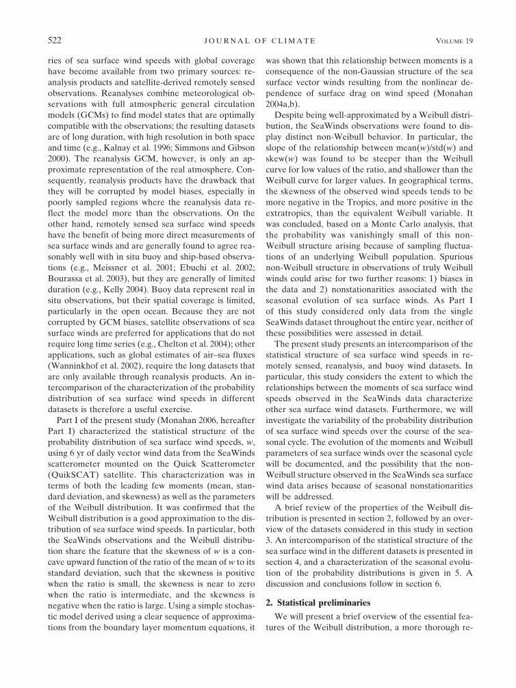
The mean, standard deviation, skewness, and kurto-sis fields of w from the SeaWinds, SSM/I, ERA-40, andNCEP–NCAR reanalysis datasets are displayed in Fig.2. The moment fields estimated from the four datasets

FIG. 1. Locations of buoys considered in this study (NDBC buoys: triangles; TAO buoys:filled circles; PIRATA buoys: asterisks).


share the same basic features. Maxima in mean(w) areevident over the Southern Ocean and in the NH mid-latitude storm tracks. Secondary maxima of the meanwind speed are observed along the equatorward flanksof the subtropical high pressure cells, and minima areevident in the equatorial doldrums and subtropicalhorse latitudes. The standard deviation of w is largest inthe midlatitude storm tracks and generally decreasesequatorward; variability is generally smallest beneaththe climatological subtropical anticyclones. A weak lo-cal maximum in std(w) lies along the intertropical con-vergence zone (ITCZ). The skewness of w is stronglypositive in the NH extratropics and along the equator-ward flank of the Southern Hemisphere (SH) westerlyjet; it is close to zero over the Southern Ocean, and it isnegative in those parts of the Tropics and subtropicscharacterized by strong and steady winds. The kurtosisof w is generally negative along the ITCZ and in theIndian Ocean, close to zero over the Southern Oceanand in much of the Tropics, and positive elsewhere.

While the moment fields estimated from the SeaWinds,SSM/I, ERA-40, and NCEP–NCAR datasets share thesame basic features in common, they differ in details.Figure 3 presents maps of the SSM/I, ERA-40, andNCEP–NCAR moment fields minus the SeaWinds mo-ment fields. It is evident that the SeaWinds mean(w)

field is generally larger than the mean(w) fields fromthe other datasets, although differences are small withmean(w) from SSM/I. Differences from the reanalysisdatasets are particularly large in the Tropics and overthe Southern Ocean. The SeaWinds std(w) field isslightly smaller than the SSM/I std(w) field in the Trop-ics and is slightly larger over the Southern Ocean. TheERA-40 std(w) is generally biased low relative to theSeaWinds std(w). Differences in std(w) between Sea-Winds and the NCEP–NCAR reanalysis are typicallysmall and spatially disorganized. The negative skew(w)in the Tropics is considerably weaker in the SSM/I andNCEP–NCAR datasets and slightly stronger in theERA-40 dataset than in the SeaWinds observations.The ERA-40 skew(w) field is also more negative overthe Southern Ocean than the skewness fields of theother datasets. Differences between kurt(w) fields esti-mated from the different datasets are larger than forthe other moment fields. In general, the SeaWindskurt(w) field is larger than the kurt(w) fields of theother datasets, although there are localized regions inwhich the sign of the difference is reversed.

Previous studies have noted that satellite observa-tions of mean sea surface wind speeds tend to be largerthan analysis or reanalysis estimates in both the Tropics(e.g., Meissner et al. 2001; Bentamy et al. 2003) and

FIG. 2. Mean, std dev, skewness, and kurtosis fields for the SeaWinds, SSM/I, ERA-40, and NCEP–NCAR sea surface wind speeddatasets. The solid line in the skewness plots is the zero contour.


Fig 2 live 4/C

over the Southern Ocean (e.g., Yuan 2004); these ear-lier results are consistent with the differences presentedin Fig. 3. Caires et al. (2004) noted that mean(w) in theTropics was higher in the ERA-40 data than in theNCEP–NCAR reanalysis data, again consistent withthe results presented in Fig. 3. Chelton and Freilich(2005) compared SeaWinds wind speed observationswith NCEP and ECMWF operational analysis fieldsand also found that in some years the ECMWF analysismean(w) is biased low relative to the SeaWindsmean(w) field, although it is also biased low relative tothe NCEP analyses.

As was noted by Chelton and Freilich (2005), someof the differences in mean(w) between the remotelysensed and reanalysis datasets may arise because satel-lite observations measure wind stress, which is thenconverted to 10-m equivalent neutral-stability windswithout accounting for stratification effects (Liu andTang 1996). Reanalysis models, on the other hand, at-tempt to simulate the actual winds at 10 m. Chelton andFreilich (2005) estimate that the difference between ac-tual 10-m winds and equivalent neutral-stability windscan account for �0.2 m s�1 of the difference betweenthe remotely sensed and simulated wind fields. Further-more, reanalysis models do not resolve small-scalestructures in sea surface temperature that modify thelocal boundary layer stability with a measurable localeffect on sea surface winds (e.g., Chelton et al. 2004).Chelton and Freilich (2005) also emphasize the fact thatremotely sensed observations of sea surface winds aresensitive to the vector velocity difference between the

ocean surface and the 10-m wind, rather than the 10-mwind itself, while reanalysis models neglect surface cur-rents and assume a rigid bottom boundary; reanalyzedwind fields will therefore be biased relative to remotelysensed winds in regions of swift surface currents (e.g.,Kelly et al. 2001, 2005). This effect may account forsome of the differences between the moment fields,particularly in the regions of relatively swift surface cur-rents around the equator and the Southern Ocean.

b. Weibull parameters

Fields of the Weibull scale and shape parameters, aand b, for each of the SeaWinds, SSM/I, ERA-40, andNCEP–NCAR surface wind speed datasets are pre-sented in Fig. 4. For each of the datasets considered, thefield of the Weibull shape parameter a has essentiallythe same structure as the field of mean(w). Further-more, all four datasets share the same overall distribu-tion of b: the Weibull shape parameter varies between2 and 3 in the NH midlatitudes, over the Indo-Pacificwarm pool, and on the equatorward flank of the SHsurface westerly jet; between 3 and 4 over the SouthernOcean; and above 4 on the equatorward flanks of thesubtropical highs, with values up to 6 over the subtropi-cal Atlantic and eastern Pacific. Maxima in b are gen-erally larger in the SeaWinds and ERA-40 surface winddata than in the SSM/I and NCEP–NCAR reanalysisdatasets.

As was discussed in Part I of this study, an essentialfeature shared by both the SeaWinds sea surfacewind observations and the Weibull distribution is

FIG. 3. Maps of the mean, std dev, skewness, and kurtosis fields of the SSM/I, ERA-40, and NCEP–NCAR datasets minus thecorresponding fields of the SeaWinds observations.


Fig 3 live 4/C

that skew(w) is a concave upward function of theratio mean(w)/std(w), such that the skewness is posi-tive where the ratio is small, near zero where theratio is intermediate, and negative where the ratio islarge. Kernel density estimates of the joint PDF of

mean(w)/std(w) with skew(w) for each of the SeaWinds,SSM/I, ERA-40, and NCEP–NCAR reanalysis datasetsare presented in Fig. 5, along with the theoretical curvefor a Weibull variable. A scatterplot of mean(w)/std(w)against skew(w) for the buoy data is presented in Fig. 6.

FIG. 4. Same as in Fig. 2, but for the Weibull a and b parameters.

FIG. 5. Kernel density estimates of the joint PDFs (contoured on logarithmic scales) of mean(w)/std(w) with skew(w) for SeaWinds,SSM/I, ERA-40, and NCEP–NCAR sea surface wind speeds. The thick black curve is the predicted relationship between moments fora Weibull variable.


Fig 4 live 4/C

Too few buoys were available for a meaningful estimateto be made of the joint PDF of mean(w)/std(w) withskew(w) from buoy data. Evidently, despite differencesin detail, all five datasets are in qualitative agreementregarding the relationship between the moments of seasurface wind speed. In particular, the theoreticalWeibull curve runs through the joint PDFs of the Sea-Winds, SSM/I, ERA-40, and NCEP–NCAR reanalysisdata, and through the scatter of the buoy data. It isdemonstrated in Part I that the relationships betweenthe fields of mean(w), std(w), and skew(w) can bequalitatively understood in terms of boundary layer dy-namics subject to fluctuating large-scale forcing andnonlinear surface drag.

There is also agreement among these five data-sets regarding deviations in the structure of windspeed PDFs from Weibull. In all datasets, the slope ofthe relationship between skew(w) and the ratiomean(w)/std(w) is steeper than that of the Weibullcurve for low values of the ratio, and it is shallower thanthat of the Weibull curve for larger values of the ratio.Using a Monte Carlo approach, it was demonstrated inPart I that the probability was vanishingly small of theapparent non-Weibull structure of the SeaWinds obser-vations arising due to sampling fluctuations of a trulyWeibull population. Similar calculations for the SSM/I,ERA-40, NCEP–NCAR reanalysis, and buoy datasets(not shown) indicate that the probability is also vanish-ingly small such that the non-Weibull structure in thesedatasets is attributable to sampling fluctuations of aWeibull variable.

To examine the geographical distribution of non-

Weibull structure in sea surface winds, maps of the ob-served skew(w) field minus the skew(w) field predictedfor a Weibull variable with the observed mean(w) andstd(w) [Eq. (4)] were computed for each of the SeaWinds,SSM/I, ERA-40, and NCEP–NCAR datasets (Fig. 7).In all four datasets, the estimated skew(w) is morenegative in the Tropics and more positive in the NHmidlatitudes than is the skewness field for the equiva-lent Weibull variable. In the reanalysis datasets, theskewness field over the Southern Ocean is more nega-tive than the skewness of the equivalent Weibull field;this is consistent with the negative biases in thesedatasets of skew(w) over the Southern Ocean evidentin Figs. 2 and 3.

FIG. 6. Scatterplot of mean(w)/std(w) vs skew(w) for NDBC(triangles), TAO (squares), and PIRATA (asterisks) buoy obser-vations. The solid curve is the predicted relationship betweenmoments for a Weibull variable.

FIG. 7. Maps of the observed SeaWinds, SSM/I, ERA-40, andNCEP–NCAR skew(w) fields minus the skew(w) fields of theequivalent Weibull variables.


Fig 7 live 4/C

In Part I of this study, it was noted that the Weibulldistribution provides a reasonable approximation to thePDF of SeaWinds sea surface wind speeds, althoughthere are large-scale differences between the observedmoment fields and those associated with best-fitWeibull distributions. The present analysis demon-strates that these differences are evident in all thedatasets under consideration and that the main featuresof the differences between observed and Weibull mo-ment fields are consistent between different datasets.

5. Seasonal variability

The analyses of the PDFs of sea surface wind speedpresented in the previous section and in Part I useddata from throughout the entire year, without regardfor seasonal variability. Considerable regional (if notglobal) seasonal evolution of the PDF of w is expected.Characterization of this seasonal variability is a basicelement of the full characterization of the PDF of seasurface wind speeds. Furthermore, it is possible that theapparent non-Weibull structure of the sea surface windspeeds discussed in the previous section is a conse-quence of this nonstationarity in the statistics of w: sea-sonal evolution in the a and b parameters of an instan-taneously Weibull variable could yield a year-round

PDF that is no longer Weibull. To assess the seasonalevolution of the probability distributions of sea surfacewinds, the SSM/I dataset is subdivided into four sea-sons: March–May (MAM); June–August (JJA); Sep-tember–November (SON), and December–February(DJF). The SSM/I dataset is used rather than the Sea-Winds observations because of its relatively long dura-tion; as was discussed in section 4, the PDFs of seasurface wind speed in the SeaWinds and SSM/I datasetsagree in their essential features. A description followsof the seasonal evolution of the statistical properties ofw, in terms of both moments and Weibull parameters.

a. Moments

The fields of mean(w), std(w), skew(w), and kurt(w)for each of the MAM, JJA, SON, and DJF seasons arepresented in Fig. 8. The seasonal cycle in mean(w) isgreatest in the midlatitudes, particularly in the North-ern Hemisphere, with the strongest mean wind speedsoccurring in the winter season (DJF in NH; JJA in SH).Annual variability in mean(w) is considerably smallerin the subtropics, with somewhat stronger mean windspeeds along the equatorward flank of the subtropicalhighs in the winter season than in the summer. An ex-ception in the subtropics is the equatorward flank of theIndian Ocean subtropical high, which displays a

FIG. 8. Same as in Fig. 2, but for each of the MAM, JJA, SON, and DJF seasons for the SSM/I data.


Fig 8 live 4/C

marked annual cycle in mean(w) associated with theAustralasian monsoon. A seasonal meridional migra-tion of the equatorial doldrums is also evident.

As was the case with mean(w), midlatitude values ofstd(w) are stronger in the winter season than in thesummer season, with a strong seasonal cycle evident inthe NH and a weaker cycle in the SH. Variability in thesubtropics is relatively weak in all seasons.

Throughout the seasonal cycle, skew(w) is positive inthe NH extratropics; in general, largest positive valuesoccur in JJA and smallest positive values occur in DJF.Conversely, skew(w) remains close to zero throughoutthe year over the Southern Ocean. The band of positiveskewness on the equatorward flank of the SH surfacewesterly jet varies in strength over the seasonal cycle inopposite phase to the cycle of mean(w) in the jet:skew(w) in this band is relatively high when the meanjet is weak, and skew(w) is relatively low when the jetis strong. In the subtropics, the region in which skew(w)is negative evolves seasonally. Generally, in the sum-mer (winter) hemisphere, this region is somewhat

larger (smaller) and the values of skew(w) are more(less) strongly negative. An exception to this tendencyis in the subtropical Indian Ocean, in which skew(w)becomes most strongly negative on the equatorwardflank of the subtropical high in the NH summer. Skew-ness of w is positive over the Indo-Pacific warm poolthroughout the year. In general, the most negative val-ues of kurt(w) in the extratropics of either hemisphereoccur in the winter season and the most positive valuesoccur in the summer season. In all seasons, the kurt(w)field is relatively noisy in comparison to the lower-order moment fields.

b. Weibull parameters

Fields of the Weibull size and shape parameters, aand b, for each of the MAM, JJA, SON, and DJF sea-sons are displayed in Fig. 9. The seasonal evolution of afollows that of mean(w), as would be expected.Throughout the seasonal cycle, values of b are between2 and 3 in the NH extratropics, over the Indo-Pacificwarm pool, and along the equatorward flank of the SH

FIG. 9. Same as in Fig. 4, but for each of the MAM, JJA, SON, and DJF seasons for theSSM/I data.


Fig 9 live 4/C

westerly jet. Over the Southern Ocean, b varies be-tween 3 and 4. In all seasons, the largest values of boccur in the subtropics, along the equatorward flanks ofthe subtropical highs where mean(w) is strong andstd(w) is relatively low; in these regions, b can exceed avalue of 5. In general, b is largest in the spring andsummer.

January and July maps of the Weibull b parameter inthe North Atlantic sector estimated from 30 yr worth ofship data were presented in Isemer and Hasse (1991).This earlier study indicated that b is close to 2 through-out the North Atlantic with the exception of a subtropi-cal band of high values (between 3 and 4) that migratedequatorward in the winter and poleward in the summer,in close agreement with the seasonal evolution of bdisplayed in Fig. 9. Conversely, the results of Pavia andO’Brien (1986, hereafter PO) differ significantly fromthe results of the present study. Pavia and O’Brien con-sidered a single year of ship observations, zonally av-eraged into four different ocean basins (Atlantic, In-dian, western Pacific, and eastern Pacific). As is dis-cussed in Part I, the data coverage in PO of the Tropicsand SH midlatitudes was sparse. The annual cycles ofthe Weibull-scale parameter a reported in PO arebroadly in agreement with the results presented in Fig.9. On the other hand, the estimates of b presented inPO are markedly different than those of the presentstudy. The values of b reported in PO are in generalconsiderably lower than those presented in Fig. 9; inparticular, the results of PO present no evidence overany of the four ocean basins of subtropical maxima in b.These maxima appear in all datasets considered in thisstudy and in all seasons, and their existence is consistentwith the regions of negatively skewed w described inthis study and in Bauer (1996). We conclude that thedifferences between the characterization of b in PO andthat of the present study, both in terms of geographicalstructure and seasonal evolution, arise because of thelimited data used in PO (leading to sampling errors)

and their use of zonal averaging (as structure in b is notzonally symmetric).

To assess whether the apparent non-Weibull struc-ture of w evident in Figs. 5–7 is a result of seasonalvariation in the Weibull parameters, the joint PDFs ofmean(w)/std(w) with skew(w) were calculated for eachof the MAM, JJA, SON, and DJF seasons (Fig. 10). Foreach season, the joint PDF is characterized by the re-lationship between moments characteristic of the fullyear (Fig. 5), such that the theoretical curve for aWeibull variable runs through the joint PDF. Evidently,the seasonal sea surface wind speeds are no lessWeibull than the full-year wind speeds. However, nei-ther are they more Weibull: as in the year-round data,for each season the slope of the relationship betweenthe ratio mean(w)/std(w) and skew(w) is steeper thanthe slope of the Weibull curve for small values of theratio and shallower for large values of the ratio. Thenon-Weibull structure characteristic of the full-yeardata is also evident in the seasonally stratified data.

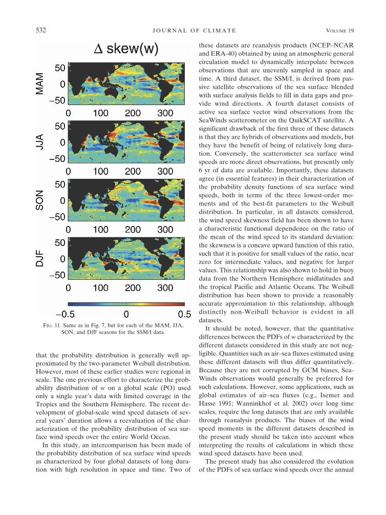
Maps of the SSM/I skew(w) field minus the equiva-lent Weibull skew(w) field obtained using the SSM/Imean(w) and std(w) fields, for each of the MAM, JJA,SON, and DJF seasons, are presented in Fig. 11. In allseasons, difference fields between the observed andWeibull fields are similar in pattern and magnitude todifference fields obtained using data from throughoutthe year (the second panel in Fig. 7). Evidently, thedeviation of the year-round PDF of w from Weibull isnot a consequence of seasonal nonstationarity: the seasurface wind speeds in each season also display consid-erable non-Weibull behavior.

6. Discussion and conclusions

A number of previous studies (e.g., PO; Isemer andHasse 1991; Bauer 1996; Pryor and Barthelmie 2002)have investigated the probability distribution of sea sur-face wind speeds, w, in which it has been demonstrated

FIG. 10. Same as in Fig. 5, but for each of the MAM, JJA, SON, and DJF seasons of the SSM/I data.


that the probability distribution is generally well ap-proximated by the two-parameter Weibull distribution.However, most of these earlier studies were regional inscale. The one previous effort to characterize the prob-ability distribution of w on a global scale (PO) usedonly a single year’s data with limited coverage in theTropics and the Southern Hemisphere. The recent de-velopment of global-scale wind speed datasets of sev-eral years’ duration allows a reevaluation of the char-acterization of the probability distribution of sea sur-face wind speeds over the entire World Ocean.

In this study, an intercomparison has been made ofthe probability distribution of sea surface wind speedsas characterized by four global datasets of long dura-tion with high resolution in space and time. Two of

these datasets are reanalysis products (NCEP–NCARand ERA-40) obtained by using an atmospheric generalcirculation model to dynamically interpolate betweenobservations that are unevenly sampled in space andtime. A third dataset, the SSM/I, is derived from pas-sive satellite observations of the sea surface blendedwith surface analysis fields to fill in data gaps and pro-vide wind directions. A fourth dataset consists ofactive sea surface vector wind observations from theSeaWinds scatterometer on the QuikSCAT satellite. Asignificant drawback of the first three of these datasetsis that they are hybrids of observations and models, butthey have the benefit of being of relatively long dura-tion. Conversely, the scatterometer sea surface windspeeds are more direct observations, but presently only6 yr of data are available. Importantly, these datasetsagree (in essential features) in their characterization ofthe probability density functions of sea surface windspeeds, both in terms of the three lowest-order mo-ments and of the best-fit parameters to the Weibulldistribution. In particular, in all datasets considered,the wind speed skewness field has been shown to havea characteristic functional dependence on the ratio ofthe mean of the wind speed to its standard deviation:the skewness is a concave upward function of this ratio,such that it is positive for small values of the ratio, nearzero for intermediate values, and negative for largervalues. This relationship was also shown to hold in buoydata from the Northern Hemisphere midlatitudes andthe tropical Pacific and Atlantic Oceans. The Weibulldistribution has been shown to provide a reasonablyaccurate approximation to this relationship, althoughdistinctly non-Weibull behavior is evident in alldatasets.

It should be noted, however, that the quantitativedifferences between the PDFs of w characterized by thedifferent datasets considered in this study are not neg-ligible. Quantities such as air–sea fluxes estimated usingthese different datasets will thus differ quantitatively.Because they are not corrupted by GCM biases, Sea-Winds observations would generally be preferred forsuch calculations. However, some applications, such asglobal estimates of air–sea fluxes (e.g., Isemer andHasse 1991; Wanninkhof et al. 2002) over long timescales, require the long datasets that are only availablethrough reanalysis products. The biases of the windspeed moments in the different datasets described inthe present study should be taken into account wheninterpreting the results of calculations in which thesewind speed datasets have been used.

The present study has also considered the evolutionof the PDFs of sea surface wind speeds over the annual

FIG. 11. Same as in Fig. 7, but for each of the MAM, JJA,SON, and DJF seasons for the SSM/I data.


Fig 11 live 4/C

cycle in the SSM/I dataset. It is found that the Weibullapproximation is equally good in each of the MAM,JJA, SON, and DJF calendar seasons, and that the de-viations from Weibull behavior evident in the full-yeardata are not simply a result of the seasonal nonstation-arity of the Weibull parameters. The present study ex-tends the result of previous studies characterizing theseasonal evolution of the sea surface wind speedWeibull parameters, which were geographically limited(e.g., Isemer and Hasse 1991) or used a dataset of toolimited a duration to yield statistically robust estimates(e.g., PO).

The present study has taken advantage of long-duration global datasets of sea surface winds with highresolution in space and time that have only recentlybecome available to produce a statistically robust char-acterization of the seasonal and geographical structureof the probability distribution of sea surface windspeeds. It is to be expected that refinements to thispicture will be made as the quality and duration of windspeed datasets improve. Given the leading-order simi-larity of the statistical properties of the four datasetsconsidered, however, it is not expected that the char-acterization of large-scale features in sea surface windspeed PDFS will change qualitatively. In particular, it isevident in all datasets and in all seasons that skew(w) isa concave upward function of the ratio mean(w)/std(w),positive where this ratio is small, close to zero wherethe ratio is intermediate, and negative where the ratio islarge. A mechanistic model presented in Part I of thisstudy is able to qualitatively characterize this relation-ship but is quantitatively inaccurate. A goal of futureresearch will be the construction of physically basedmodels that can quantitatively reproduce the robust re-lationships between statistical moments of the sea sur-face wind speeds that have been demonstrated in thisstudy.

Acknowledgments. The author acknowledges sup-port from the Natural Sciences and Engineering Re-search Council of Canada, from the Canadian Founda-tion for Climate and Atmospheric Sciences, and fromthe Canadian Institute for Advanced Research EarthSystem Evolution Program. The author would also liketo thank Philip Sura and two anonymous refereeswhose comments significantly improved this manu-script.

REFERENCES

Atlas, R., R. Hoffman, S. Bloom, J. Jusem, and J. Ardizzone,1996: A multiyear global surface wind velocity dataset usingSSM/I wind observations. Bull. Amer. Meteor. Soc., 77, 869–882.

Bauer, E., 1996: Characteristic frequency distributions of re-motely sensed in situ and modelled wind speeds. Int. J. Cli-matol., 16, 1087–1102.

Bentamy, A., K. B. Datsaros, A. M. Mestas-Nuñez, W. M. Dren-nan, E. B. Forde, and H. Roquet, 2003: Satellite estimates ofwind speed and latent heat flux over the global oceans. J.Climate, 16, 637–656.

Bourassa, M. A., D. M. Legler, J. J. O’Brien, and S. R. Smith,2003: SeaWinds validation with research vessels. J. Geophys.Res., 108, 3019, doi:10.1029/2001JC001028.

Caires, S., A. Sterl, J.-R. Bidlot, N. Graham, and V. Swail, 2004:Intercomparison of different wind–wave reanalyses. J. Cli-mate, 17, 1893–1912.

Chelton, D. B., and M. H. Freilich, 2005: Scatterometer-basedassessment of 10-m wind analyses from the operationalECMWF and NCEP numerical weather prediction models.Mon. Wea. Rev., 133, 409–429.

——, M. G. Schlax, M. H. Freilich, and R. F. Milliff, 2004: Satellitemeasurements reveal persistent small-scale features in oceanwinds. Science, 303, 978–983.

Donelan, M., W. Drennan, E. Saltzman, and R. Wanninkhof,Eds., 2002: Gas Transfer at Water Surfaces. Amer. Geophys.Union, 383 pp.

Ebuchi, N., H. C. Graber, and M. J. Caruso, 2002: Evaluation ofwind vectors observed by QuikSCAT/SeaWinds using oceanbuoy data. J. Atmos. Oceanic Technol., 19, 2049–2062.

Erickson, D. J., and J. A. Taylor, 1989: Non-Weibull behavior ob-served in a model-generated global surface wind field fre-quency distribution. J. Geophys. Res., 94, 12 693–12 698.

Isemer, H., and L. Hasse, 1991: The scientific Beaufort equivalentscale: Effects on wind statistics and climatological air–sea fluxestimates in the North Atlantic Ocean. J. Climate, 4, 819–836.

Jet Propulsion Laboratory, cited 2001: SeaWinds on QuikSCATLevel 3: Daily, gridded ocean wind vectors. Tech. Rep.JPL PO.DAAC Product 109, California Institute of Technol-ogy. [Available online at http://podaac.jpl.nasa.gov:2031/DATASET_DOCS/qscat_L3.html.]

Jones, I. S., and Y. Toba, Eds., 2001: Wind Stress over the Ocean.Cambridge University Press, 307 pp.

Kalnay, E., and Coauthors, 1996: The NCEP/NCAR 40-Year Re-analysis Project. Bull. Amer. Meteor. Soc., 77, 437–471.

Kelly, K. A., 2004: Wind data: A promise in peril. Science, 303,962–963.

——, S. Dickinson, M. J. McPhaden, and G. C. Johnson, 2001:Ocean currents evident in ocean wind data. Geophys. Res.Lett., 28, 2469–2472.

——, ——, and G. C. Johnson, 2005: Comparisons of scatterom-eter and TAO winds reveal time-varying surface currents forthe tropical Pacific Ocean. J. Atmos. Oceanic Technol., 22,735–745.

Krasnopolsky, V., L. Breaker, and W. Gemmill, 1995: A neuralnetwork as a nonlinear transfer function model for retrievingsurface wind speeds from the SSM/I. J. Geophys. Res., 100,11 033–11 045.

Liu, W. T., and W. Tang, 1996: Equivalent neutral wind. Tech.Rep., JPL Publication 96-17, Pasadena, CA, 8 pp.

Meissner, T., D. Smith, and F. Wentz, 2001: A 10 year intercom-parison between collocated Special Sensor Microwave Im-ager oceanic surface wind speed retrievals and global analy-ses. J. Geophys. Res., 106, 11 731–11 742.

Monahan, A. H., 2004a: Low-frequency variability of the statisti-cal moments of sea-surface winds. Geophys. Res. Lett., 31,L10302, doi:10.1029/2004GL019599.


——, 2004b: A simple model for the skewness of global sea sur-face winds. J. Atmos. Sci., 61, 2037–2049.

——, 2006: The probability distribution of sea surface windspeeds. Part I: Theory and SeaWinds observations. J. Cli-mate, 19, 497–520.

Pavia, E. G., and J. J. O’Brien, 1986: Weibull statistics of windspeed over the ocean. J. Climate Appl. Meteor., 25, 1324–1332.

Pryor, S., and R. Barthelmie, 2002: Statistical analysis of flowcharacteristics in the coastal zone. J. Wind Eng. Ind. Aero-dyn., 90, 201–221.

Simmons, A., and J. Gibson, 2000: The ERA-40 project plan.ERA-40 Project Rep. Series 1, ECMWF, Reading, UnitedKingdom, 63 pp.

Thompson, K., R. Marsden, and D. Wright, 1983: Estimation oflow-frequency wind stress fluctuations over the open ocean.J. Phys. Oceanogr., 13, 1003–1011.

Tuller, S. E., and A. C. Brett, 1984: The characteristics of wind

velocity that favor the fitting of a Weibull distribution in windspeed analysis. J. Climate Appl. Meteor., 23, 124–134.

Wanninkhof, R., 1992: Relationship between wind speed and gasexchange over the ocean. J. Geophys. Res., 97, 7373–7382.

——, and W. R. McGillis, 1999: A cubic relationship betweenair-sea CO2 exchange and wind speed. Geophys. Res. Lett.,26, 1889–1892.

——, S. C. Doney, T. Takahashi, and W. R. McGillis, 2002: Theeffect of using time-averaged winds on regional air-sea CO2

fluxes. Gas Transfer at Water Surfaces, M. A. Donelan et al.,Eds., Amer. Geophys. Union, 351–356.

Wentz, F., 1997: A well-calibrated ocean algorithm for SpecialSensor Microwave/Imager. J. Geophys. Res., 102, 8703–8718.

Wright, D. G., and K. R. Thompson, 1983: Time-averaged formsof the nonlinear stress law. J. Phys. Oceanogr., 13, 341–345.

Yuan, X., 2004: High-wind-speed evaluation in the Southern Ocean.J. Geophys. Res., 109, D13101, doi:10.1029/2003JD004179.


the probability distribution of sea surface wind speeds

Documents