the privacy/security tradeoff for multiple secure … · chapter 1. introduction 2 the problem of...
TRANSCRIPT

The Privacy/Security Tradeoff for Multiple Secure Sketch BiometricAuthentication Systems
by
Adina Rebecca Goldberg
A thesis submitted in conformity with the requirementsfor the degree of Master of Applied Science
Graduate Department of Electrical and Computer EngineeringUniversity of Toronto
c© Copyright 2015 by Adina Rebecca Goldberg

Abstract
The Privacy/Security Tradeoff for Multiple Secure Sketch Biometric Authentication Systems
Adina Rebecca Goldberg
Master of Applied Science
Graduate Department of Electrical and Computer Engineering
University of Toronto
2015
When designing multiple biometric authentication systems, there is tension between minimizing
privacy leakage and maximizing security. This work studies the tradeoff between the two measures for
jointly designed “secure sketch” systems. Secure sketch is a biometric system architecture where, as
with error-correcting codes, a system is characterized by a parity-check matrix over a finite field. Single
systems have been widely researched, but little is known about the privacy and security of joint designs,
when leakage of one system can compromise the security of the others. This work introduces worst-case
measures of privacy leakage and security for sets of systems and studies the tradeoff between them:
First by studying the algebraic structure of the problem, then through a continuous relaxation of the
problem (in a restricted case) and performing optimizations. An analytic expression for the tradeoff in
that restricted case is proposed which aligns with simulation results.
ii

Acknowledgements
First and foremost, I’d like to thank my research supervisor, Professor Stark Draper, for all of his support
and guidance, and always encouraging me to dig deeper. He helped me keep the big picture in mind while
continuing to put one foot in front of the other. For that, I’m very grateful. Second, I’d like to thank
my research group: Yanina Shkel, Xishuo Liu, and Yanpei Liu for helping me navigate through some
earlier versions of this work, and Mitchell Wasson, for helping me get through course development while
I was trying to tie together the loose ends of this research. Third, I’m grateful to my thesis committee
for taking the time to read this document.
I’d also like to thank the people at U of T who helped me get comfortable with topics I knew little
about at the beginning. In particular, I’m grateful to Professor Frank Kschischang for the early chat we
had about subspace structure and the L = 1 case. I’m also grateful to Steven Rayan for meeting with
me to chat about the Grassmann graph and the algebra side of things. I’d additionally like to thank
Professor Wei Yu for teaching an excellent course on convex optimization, which played a large role in
this work.
I’d like to acknowledge that this work was completed with the support of an NSERC CGS award
and an OGS award.
I’m lucky enough to have some close friends with a good grasp of the mathematical concepts behind
this thesis. A big thanks to Melkior Ornik for talking through some of the proofs with me and being
an excellent producer of counterexamples to my sometimes over-optimistic ideas. I’m very grateful to
Elliot Cheung for talking through proofs with me as well, for getting me pizza, and for helping me push
through the last bit of writing when I couldn’t stand to look at this document anymore.
Finally, I’d like to thank my family for encouraging me not to quit graduate school a few months in,
and for being supportive and fun (but occasionally a bit too distracting) whenever research got stressful.
iii

Contents
1 Introduction 1
1.1 Motivation and background . . . . . . . . . . . . . . . . . . . . . . . . . . . . . . . . . . . 1
1.1.1 Privacy and security of biometric authentication systems . . . . . . . . . . . . . . 1
1.1.2 Secure sketch systems . . . . . . . . . . . . . . . . . . . . . . . . . . . . . . . . . . 2
1.1.3 Related problems in other areas . . . . . . . . . . . . . . . . . . . . . . . . . . . . . 3
1.2 Definitions . . . . . . . . . . . . . . . . . . . . . . . . . . . . . . . . . . . . . . . . . . . . . 4
1.3 Problem statement . . . . . . . . . . . . . . . . . . . . . . . . . . . . . . . . . . . . . . . . 6
1.4 Organization . . . . . . . . . . . . . . . . . . . . . . . . . . . . . . . . . . . . . . . . . . . 6
2 The general case 7
2.1 Graphs . . . . . . . . . . . . . . . . . . . . . . . . . . . . . . . . . . . . . . . . . . . . . . . 7
2.1.1 Grassmann graph . . . . . . . . . . . . . . . . . . . . . . . . . . . . . . . . . . . . . 7
2.1.2 Subspace Hasse diagram . . . . . . . . . . . . . . . . . . . . . . . . . . . . . . . . . 8
2.2 Symmetry . . . . . . . . . . . . . . . . . . . . . . . . . . . . . . . . . . . . . . . . . . . . . 11
2.2.1 Size of design space . . . . . . . . . . . . . . . . . . . . . . . . . . . . . . . . . . . 11
2.2.2 Equivalence of designs . . . . . . . . . . . . . . . . . . . . . . . . . . . . . . . . . . 12
3 Optimization in the fixed-basis case 14
3.1 Fixed-basis designs . . . . . . . . . . . . . . . . . . . . . . . . . . . . . . . . . . . . . . . . 14
3.1.1 Effects of restriction to a fixed basis . . . . . . . . . . . . . . . . . . . . . . . . . . 14
3.1.2 Representation of fixed-basis designs . . . . . . . . . . . . . . . . . . . . . . . . . . 15
3.1.3 Tradeoff by optimization . . . . . . . . . . . . . . . . . . . . . . . . . . . . . . . . . 16
3.2 Relaxation . . . . . . . . . . . . . . . . . . . . . . . . . . . . . . . . . . . . . . . . . . . . . 17
3.3 Simplification . . . . . . . . . . . . . . . . . . . . . . . . . . . . . . . . . . . . . . . . . . . 21
3.3.1 Variable reduction . . . . . . . . . . . . . . . . . . . . . . . . . . . . . . . . . . . . 21
3.3.2 Constraint reduction . . . . . . . . . . . . . . . . . . . . . . . . . . . . . . . . . . . 23
3.4 The privacy-security tradeoff . . . . . . . . . . . . . . . . . . . . . . . . . . . . . . . . . . 27
3.4.1 A form for optimal solutions . . . . . . . . . . . . . . . . . . . . . . . . . . . . . . 28
3.4.2 Expressions for the tradeoff . . . . . . . . . . . . . . . . . . . . . . . . . . . . . . . 30
4 Conclusions 34
4.1 Summary of results . . . . . . . . . . . . . . . . . . . . . . . . . . . . . . . . . . . . . . . . 34
4.2 Directions for future work . . . . . . . . . . . . . . . . . . . . . . . . . . . . . . . . . . . . 34
iv

A Plots 35
Appendix 36
Bibliography 36
v

List of Figures
1.1 Block diagram of a keyless secure sketch system, modeled on [12]. . . . . . . . . . . . . . . 2
2.1 The subspace Hasse diagram, H2(3). . . . . . . . . . . . . . . . . . . . . . . . . . . . . . . 9
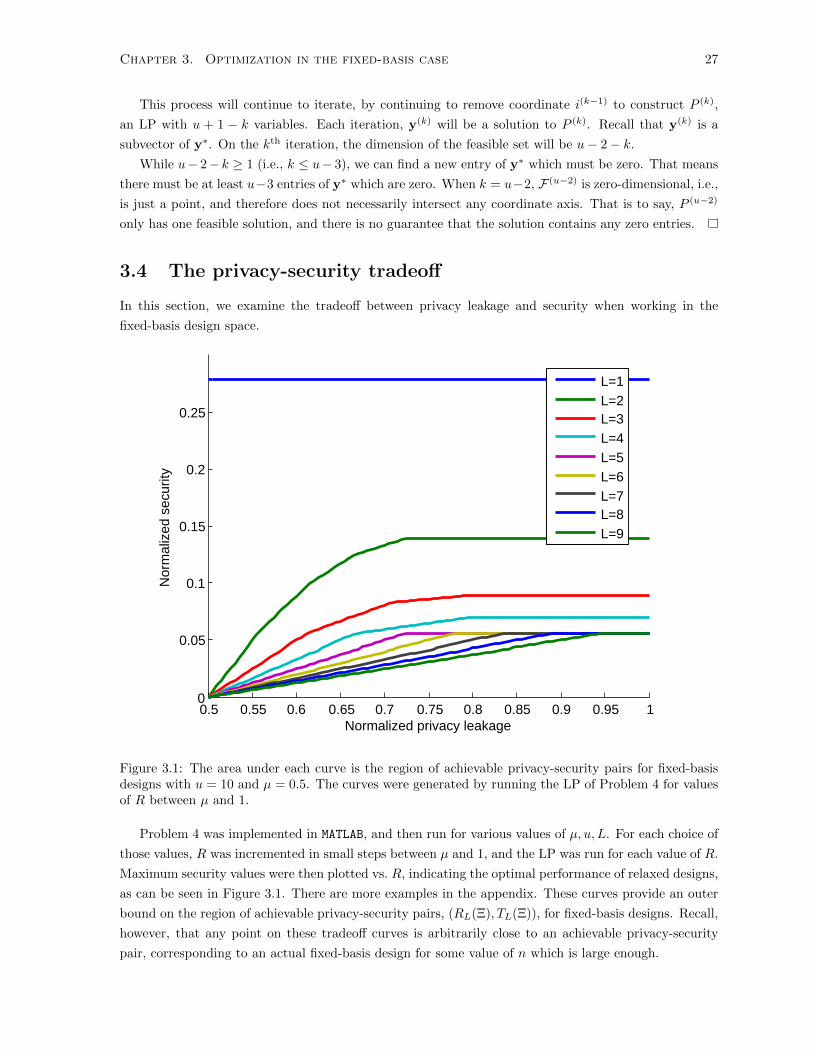
3.1 The area under each curve is the region of achievable privacy-security pairs for fixed-basis
designs with u = 10 and µ = 0.5. The curves were generated by running the LP of
Problem 4 for values of R between µ and 1. . . . . . . . . . . . . . . . . . . . . . . . . . 27
3.2 This is Figure 3.1, with the analytic predictions of Theorem 22 superimposed for u = 10,
µ = 0.5. Note that the predicted points align exactly with the optimization results. . . . . 33
A.1 Achievable privacy-security pairs for fixed-basis designs with u = 10 and µ = 0.25 from
optimization, with predictions from Theorem 22 superimposed. . . . . . . . . . . . . . . 35
A.2 Achievable privacy-security pairs for fixed-basis designs with u = 6 and µ = 0.5 from
optimization, with predictions from Theorem 22 superimposed. . . . . . . . . . . . . . . 35
A.3 Achievable privacy-security pairs for fixed-basis designs with u = 15 and µ = 0.8 from
optimization, with predictions from Theorem 22 superimposed. . . . . . . . . . . . . . . 36
A.4 Achievable privacy-security pairs for fixed-basis designs with u = 15 and µ = 0.1 from
optimization, with predictions from Theorem 22 superimposed. . . . . . . . . . . . . . . 36
vi

Chapter 1
Introduction
1.1 Motivation and background
Applications of biometrics is currently a large and popular area of research. Due to advances in the
past few decades in imaging technology, big data, and machine learning, the science fiction of the past
is quickly becoming the science of the future. The field of biometrics has experienced contributions
from a variety of disciplines, including computer science [1], biology [2], and information theory [3]. The
applications are diverse, ranging from healthcare [4] to robotics [5] to network security [6] and more.
In particular, the use of biometrics for authentication is becoming more widespread. Robust, accurate,
efficient, private, and secure methods and protocols are in high demand. Varying degrees of robustness,
accuracy, and efficiency are age-old requirements on virtually all algorithms and computer protocols.
Privacy and security, on the other hand, are requirements that are respectively unique to working with
sensitive data, and performing access control, both of which are aspects of biometric authentication.
1.1.1 Privacy and security of biometric authentication systems
This work deals with privacy and security of biometric authentication systems. Privacy and security
are closely related concepts, but the distinction between the two is crucial to this work. When we
refer to privacy, we mean keeping sensitive data a secret from the public. When we refer to security,
we mean barring unauthorized individuals from gaining access to a resource. It used to be the case
that privacy and security were mostly tangible, physical concerns. Privacy screens could keep people’s
lives hidden from prying eyes. Fences and locks could keep property and belongings secure. In the
modern world, information is becoming increasingly important, but is also becoming increasingly easy
to manipulate, duplicate and transfer. It is paramount for us to enhance our understanding of virtual
privacy and security. This is especially the case for biometric systems, where the use of biometric data
puts identities at risk and makes it possible to track people’s actions and preferences.
This work centers on designing multiple authentication systems for the same user. In the multi-
system case, it may be tempting to design each system to perform well independently, without taking
into account the fact that the infiltration of one system can actually ease the compromise of the others.
Since the systems use the same biometric data, they cannot be considered to function independently. To
get a realistic idea of privacy and security levels of jointly designed biometric authentication systems, it
is necessary to consider joint privacy measures and joint security measures.
1

Chapter 1. Introduction 2
The problem of balancing privacy and security in multiple biometric systems has already been ap-
proached from an information theoretic angle, by Lai et al. in [7, 8]. Their measures of privacy and
security are based on mutual information. Conversely, our work approaches the problem from a deter-
ministic angle, using measures of privacy and security that derive from the number of bits discovered by
an attacker in a worst-case scenario. Not many other authors have worked on joint privacy leakage and
security of multiple biometric authentication systems.
Privacy and security of single biometric systems, however, is explored by many authors. In [9],
Ratha et al. discuss the advantages and disadvantages (from a privacy and security standpoint) of using
biometrics for authentication, highlighting where biometric systems’ vulnerabilities lie, and emphasizing
the importance of privacy in the design of biometric systems. A recent book by Campisi [10] is a
compilation of a variety of research focusing on privacy and security of single biometric systems. In
particular, the chapter in that book by Ignatenko and Willems [11] has close ties with the work presented
here. In their chapter, Ignatenko and Willems find a region of achievable privacy-security pairs, but only
for a single system, and they assume a Gaussian biometric. In contrast, we look at multiple systems and
assume an i.i.d. Bernoulli( 12 ) feature vector. In [12], Wang et al. provide a framework for studying the
privacy-security tradeoff in a biometric system, and perform analysis for single systems. Towards the
end of their paper, they extend their framework to multiple systems, and pose the problem of finding a
similar tradeoff when multiple systems are involved. It was that open problem that led to this work.
1.1.2 Secure sketch systems
A ·Enrolment
+ minW :HW=s′⊕s
wt(W )
· Authentication
H
D
s
s′
wt(W )
Figure 1.1: Block diagram of a keyless secure sketch system, modeled on [12].
There are many ways to implement biometric authentication. We work with secure sketch authenti-
cation, following the definition of a keyless1 secure sketch system used in [12].
When a user enrols in a secure sketch system, the user’s biometric data is pre-processed into a q-ary
feature vector, A, of length n, which can be modelled as an independent and identically distributed
(i.i.d.) uniform random process on q symbols. The pre-processing is an important step, but is not
discussed in this work. It is only relevant here in that it produces uniformly distributed feature vectors,
which are necessary for the validity of the authentication procedure. For a discussion of feaure extraction
algorithms that approximately yield such statistics for fingerprint biometrics, see [13]. A is then mapped
1We assume each biometric system has the same single user for the purposes of this chapter, but the results can easilybe extended to multiple users by requiring users first to identify themselves with a secret key. A multi-user system with aunique key entered is essentially a single user system.

Chapter 1. Introduction 3
linearly by the matrix H in Fm×nq to a length-m q-ary vector, s = HA, that is referred to as the
syndrome2 (or template) of A. The system stores the vector s.
At the time of authentication, new biometric data is extracted and pre-processed, to produce a q-ary
vector D. D is also mapped to a syndrome, s′ = HD, and if D is close enough to A, then authentication
is successful. If the authenticator is the legitimate user, then D can be modelled as the output of a q-ary
symmetric channel3, where A is the input. Formally, the system performs the following minimization,
to estimate A⊕D:
wt(W ) = minW :HW=s′⊕s
wt(W ), (1.1)
where wt(W ) is the Hamming weight of W . Then, if wt(W ) is below some threshold, the authentication
succeeds. Otherwise, the user is turned away. Both enrolment and authentication are depicted in Figure
1.1.
It’s useful to note that authentication is analogous to syndrome decoding. A can be thought of as
the sent codeword. D can be thought of as the received word. The coset associated with the syndrome
s can be thought of as a shifted “code”. Decoding to another codeword shouldn’t happen, just as
authenticating an individual outside some ball surrounding A shouldn’t happen.
In this work, we discuss how to design sets of secure sketch systems by selecting H for each system.
We need to be able to measure the privacy and security of our designs. We’ve already said what privacy
and security mean in general, but now we will give a brief explanation of the privacy leakage and security
measures we use in our work. Formal definitions will follow in Section 1.2. Privacy leakage and security
are regarded here as measures of information, measured in bits. We will use the term security (of an
unleaked system with respect to a set of leaked systems) to refer to the amount of additional information
about a user’s feature vector that an intelligent attacker would need to learn or guess in order to gain
access to the system. We will use the term privacy leakage (of a set of leaked systems) to refer to the
amount of information about a user’s feature vector that would be known to an attacker in the case that
the attacker learned the templates stored in each system. Once we are able to measure privacy leakage
and security, we can then explore the tension between these measures when jointly designing multiple
secure sketch systems.
1.1.3 Related problems in other areas
Our problem framing has some interesting similarities to a few other areas of research. One thread of
work that is highly relevant to a special case of our problem is the work of Koetter and Kschischang in
[14], followed by the work of Khaleghi et al. on subspace codes in [15]. In the context of our problem,
these works provide a full analysis of converse and achievability bounds on designs when we only allow
one system to be compromised, i.e., L = 1. Each codeword in [15] would correspond to one system in
our setting. As we will see, for L = 1 privacy leakage is constant and security of one system with respect
to another is simply the injection distance between them.
Another of these areas is distributed storage, as explored in [16, 17]. The goal in distributed storage
is to store redundant information on a set of distributed servers in a way that strikes a balance between
two competing objectives. On the one hand, it is desirable to have high storage efficiency, as measured by
2The terminology comes from error-correcting codes.3A q-ary symmetric channel has input alphabet and output alphabet consisting of the same q symbols. A symbol goes
to itself with probability 1− p, and to any other symbol with probability pq−1
, for some p ∈ [0, 1].

Chapter 1. Introduction 4
the total number of bits stored. On the other hand, the system should be efficiently reparable in the face
of losing the data on some subset of the servers, in that the bandwidth required to replace or regenerate
the information on a lost server should be minimal. We have already seen that the subspace codes of
[14], used in a particular type of network coding, correspond to a special case of our design problem.
Hence, it’s natural that distributed storage, which relies on network coding as well, should be in some
way related to our problem. In our problem as well as in distributed storage, there are two competing
measures which loosely relate to the amount of redundant information stored. In each case, one measure
responds well to having a lot of redundancy (privacy leakage and bandwidth efficiency) and one responds
well to having little redundancy (security and storage efficiency). Additionally, in both problems, the
way the redundancy is structured is of crucial importance. However, one discrepancy between the two
problems is that we want to avoid reconstruction of the user’s biometric, whereas distributed storage
looks to facilitate source reconstruction. Another difference is that in the distributed storage setting,
server losses are modelled as random erasures, whereas in our setting, systems are strategically targeted
by an intelligent attacker.
A third related area is that of secret sharing, introduced by Shamir in [18]. In secure secret sharing,
the goal is to store a secret in a distributed way among a set of participants, such that it’s impossible for
a subset of fewer than t participants to obtain any information about the value of the secret. This idea
is loosely linked to the idea of privacy in our problem, in that the goal is to distribute biometric data
among the systems so that if an attacker breaks into a small number of them, he should have tremendous
difficulty reconstructing the user’s biometric. The requirements of the secret sharing problem are quite
different, however. Secure secret sharing requires zero information to be knowable by a set of fewer than
t participants, and relies on randomness to do this. In contrast, the information stored in our systems
is non-random, and even compromising a single system may provide partial information to an attacker.
1.2 Definitions
We now define terms and introduce notation that will be used in the remainder of this work.
Definition 1. A system refers to a full-rank m × n matrix, Hi, with entries in Fq, with system size
given by m, where m < n.
We will also use the word ‘system’ to refer to the associated nullspace of Hi, denoted Vi = null(Hi) =
{v ∈ Fnq | Hiv = 0}. The intended meaning will be clear from context. Note that dim(Vi) = n−m.
Definition 2. A matrix design, H = (H1, . . . ,Hu), is a tuple of u systems. Likewise, the corresponding
subspace design is V = (V1, . . . , Vu) where each Vi = null(Hi).
Given a set, S, of indices of leaked systems, we define privacy leakage and security as follows.
Definition 3. The privacy leakage of S, denoted r(S,H), is given by
r(S,H) = rank(vsi∈S(Hi)) (1.2)
where vsi∈S(Hi) is the matrix obtained by vertically concatenating all matrices Hi such that i ∈ S.
Privacy leakage measures the amount of information4 an attacker has about a user’s biometric from
knowing the syndromes si, i ∈ S.
4We are assuming here that A is a uniform i.i.d. random process. If we don’t have ideal source statistics, the general

Chapter 1. Introduction 5
By a slight abuse of notation, we will also allow privacy leakage to take the corresponding subspace
design V as its second argument, instead of H. In that case
r(S,V) = n− dim
(⋂i∈S
Vi
)(1.3)
is an equivalent expression for the privacy leakage of S.
Definition 4. The security of the jth system with respect to S, denoted tj(S,H), and given by
tj(S,H) = r(S ∪ {j},H)− r(S,H) (1.4)
is the amount of additional information an attacker would need in order to gain access to the jth system.
Again, by a slight abuse of notation, when working with the corresponding subspace design, V,
tj(S,V) = dim(⋂i∈S
Vi)− dim(Vj ∩⋂i∈S
Vi) (1.5)
is an equivalent expression for the security of the jth system with respect to S. This follows directly
from the definition of security and the expression for privacy leakage in terms of V.
We will now introduce worst-case privacy and security measures. For the purpose of measuring
worst-case privacy leakage and security, we assume a maximum number of leaked systems, L ∈ Z, where
1 ≤ L < u.
Definition 5. The worst-case privacy leakage of a design, H, is denoted RL(H) and given by
RL(H) = maxS⊆{1,...,u}|S|=L
r(S,H). (1.6)
Definition 6. The worst-case security of a design, H, is denoted TL(H) and given by
TL(H) = minS⊆{1,...,u}|S|=L
minj /∈S
tj(S,H). (1.7)
Sometimes, it’s useful to compare the performance of designs for different feature vector lengths, i.e.,
different values of n. Accordingly, we define normalized measures:
Definition 7. The normalized worst-case privacy leakage of a design, H, is denoted RL(H) and given
by RL(H) = 1nRL(H).
Definition 8. The normalized worst-case security of a design, H, is denoted TL(H) and given by
TL(H) = 1nTL(H).
Replacing H with V in the above four definitions yields the worst-case and normalized worst-case
measures in terms of the corresponding subspace design.
A design, H, has a corresponding privacy-security pair, given by (RL(H), TL(H)) and a corresponding
normalized privacy-security pair, given by (RL(H), TL(H)).
expression for r(S,H) is given by h(A) − h(A|{HiA = si|i ∈ S}), where h(·) is the binary entropy function (in the casethat q = 2). If the source sequence has dependence in it, privacy leakage would be less than that of an independent source,and security would also be less.

Chapter 1. Introduction 6
Definition 9. We call a pair (r, t) an achievable privacy-security pair for fixed values of n,m, u, and L if
there exists H such that (r, t) = (RL(H), TL(H)). Similarly, we call a pair (r, t) an achievable normalized
privacy-security pair if there exists H such that (r, t) = (RL(H), TL(H)).
One might expect that if an (r, t) pair is achievable, then all pairs with greater privacy leakage or
lower security would also be achievable. However, due to the dependent relationship between the privacy
and security measures, there are cases where this is not true.
1.3 Problem statement
The aim of this thesis is to reveal the nature of the relationship between worst-case privacy leakage
and worst-case security. Specifically, we want to understand the design space by characterizing its
structure. We want to know when distinct designs share the same privacy-security pair. We also want
to characterize the region of achievable privacy-security pairs.
1.4 Organization
In Chapter 2, we look at the general design space, where biometric systems are characterized by arbitrary
(n−m) dimensional subspaces of Fnq . In Section 2.1, we use graphs and the theory of vector spaces over
finite fields in order to better understand the structure of our design space. We then see in Section 2.2
that the general design space is fairly large. We identify some types of equivalence between designs that
demonstrate we are really dealing with a smaller space. However, we still lack efficient ways to search
or optimize over the general space.
For that reason, in Chapter 3 we restrict ourselves to a special case of the problem, where we design
systems from a fixed basis of Fnq . First, in Section 3.1, we introduce fixed-basis designs along with
a simpler representation for systems. We formalize the problem of finding a tradeoff between privacy
leakage and security, when working with fixed-basis designs. Then, in Section 3.2, we relax that problem
to turn it into a linear program (LP). The LP obtained has exponentially many variables and constraints
in the number of systems. In Section 3.3, we reduce the LP to an equivalent LP which has linearly many
variables and constraints in the number of systems. We also prove that at most three variables are non-
zero in an optimal solution to the LP. Finally, in Section 3.4, we look at the tradeoff between privacy
leakage and security obtained by implementing the LP from the previous section. We find that the
solutions to the LP follow a regular pattern, and we conjecture that this pattern is optimal. Assuming
the truth of the conjecture, we are able to analytically construct the privacy-security tradeoff for fixed-
basis designs. This construction matches the results of our earlier optimizations, lending support to the
conjecture.
To conclude, in Chapter 4 we summarize our results, offer some open problems and future directions
for this work, and acknowledge those who aided in the completion of this thesis.

Chapter 2
The general case
In this chapter, we look at the underlying structure of the design space, and find ways to use that
structure in order to find good designs. In this chapter, we refer to systems by their corresponding
nullspace.
2.1 Graphs
There are two graphs that are of particular interest to us in our journey to understand the relationship
between the worst case privacy leakage and the worst case security of designs.
2.1.1 Grassmann graph
Definition 10. The Grassmann graph, denoted Gq(n, k), is the graph with vertex set consisting of all
k-dimensional subspaces of Fnq , with an edge between nodes U and V if dim(U ∩ V ) = k − 1.
The distance between two nodes U and V in Gq(n, k) is known as the injection distance, and cor-
responds to the least number of basis vector swaps one would need in order to take a basis for U and
transform it into a basis for V .
Note 1. The injection distance is a metric. For proof, see [19].
Let k = n−m. Selecting a subspace design, V, is equivalent to choosing u nodes in Gq(n, k) (possibly
with repetition). We would like to express RL(V) and TL(V) in terms of distances on Gq(n, k), so that
we can reframe our entire problem as a problem about Gq(n, k).
In the case that L = 1, we can indeed do this. For L = 1, we have
R1(V) = maxi∈{1,...,u}
r({i},V)
= maxi∈{1,...,u}
n− dim(Vi)
= maxi∈{1,...,u}
n− k
= n− k = m.
(2.1)
7

Chapter 2. The general case 8
Note that privacy leakage is constant with respect to the choice of V. For security, we have
T1(V) = mini 6=j
i,j∈{1,...,u}
tj({i},V)
= mini 6=j
i,j∈{1,...,u}
r({i, j},V)− r({i},V)
= mini 6=j
i,j∈{1,...,u}
n− dim(Vi ∩ Vj)− n+ dim(Vi)
= mini 6=j
i,j∈{1,...,u}
k − dim(Vi ∩ Vj)
= mini 6=j
i,j∈{1,...,u}
d(Vi, Vj),
(2.2)
where d(·, ·) is the distance in Gq(n, k), and the last step is proven in [15].
That is to say, for L = 1, our problem is equivalent to selecting u nodes in Gq(n, k) to maximize the
minimum pairwise distance between nodes. This problem is shown in [20] to be NP-complete for general
graphs. In the case of the Grassmann graph, further analysis can be found in [15].
In the case that L > 1, our security measure depends on intersections of more than two subspaces.
Pairwise intersection (or sum) information is not enough. To compute T2(V), for example, we need to
know either dim(U ∩ V ∩W ) or dim(U + V + W ) for all {U, V,W} ⊆ V. This information cannot be
learned from Gq(n, k).
2.1.2 Subspace Hasse diagram
Definition 11. The subspace Hasse diagram, denoted Hq(n), is a directed graph with vertex set con-
sisting of all subspaces of Fnq , with an edge going from U to V if U ⊆ V and dim(V ) = dim(U) + 1.
Note 2. Hq(n) is a lattice with n + 1 levels, where the level of each node is the dimension of the
corresponding subspace (beginning from level 0). We refer to following an edge to a higher (lower) level
as “travelling up” (“travelling down”).
Lemma 1. Given nodes U, V of Hq(n), let P be a path from U to V . Let Nup(P ) and Ndown(P ) be the
number of edges travelled up and down in P . Then
dim(U) +Nup(P ) = dim(V ) +Ndown(P ).
Proof. Let N be the length of P . We prove this result by induction on N .
If N = 1, there are two cases.
Nup(P ) = 1, Ndown(P ) = 0: Then there is an edge between U and V , and U ⊆ V . Therefore, dim(U) +
1 = dim(V ).
Nup(P ) = 0, Ndown(P ) = 1: Then there is an edge between U and V , and U ⊇ V . Therefore, dim(U) =
dim(V ) + 1.
Now assume the result holds for all paths of length N . We show that it is true for P of length N + 1.
Let P1 be a path consisting of the first N edges of P . P1 is therefore a path from U to some node which

Chapter 2. The general case 9
Figure 2.1: The subspace Hasse diagram, H2(3).
we shall denote W . By assumption, we have that
dim(U) +Nup(P1) = dim(W ) +Ndown(P1).
Let P2 be the remainder of P from W to V . Note that P2 has only one edge. From the base case, we
have that
dim(W ) +Nup(P2) = dim(V ) +Ndown(P2).
Adding these two equations gives
dim(U) +Nup(P ) = dim(V ) +Ndown(P ),
since Nup(P1) +Nup(P2) = Nup(P ) and likewise for Ndown(·).
Recall that the sum of two subspaces, denoted U+V , is defined as the set {u+v|u ∈ U,v ∈ V }. Note
that U + V is a subspace. Further, note that an equivalent definition of U + V is the unique minimal
dimension subspace containing both U and V .
Recall as well that the intersection of two subspaces, denoted U ∩ V , is a subspace. An equivalent
definition of U ∩ V is the unique maximal dimension subspace contained in both U and V .
To find U +V in the subspace Hasse diagram, we need to look for a common ancestor of U and V on
the lowest possible level. This node is also known as the join of U and V . Similarly, to find U ∩ V , we
need to find a common descendant of U and V on the highest possible level. This node is also known as
the meet of U and V . Since the dimension of a subspace is equal to the level of its corresponding node
in Hq(n), we can use Hq(n) to find dimensions of sums and intersections of any number of subspaces.
With the ability to find sums and intersections of subspaces, we obtain the following results on
privacy leakage and security in Hq(n).
Theorem 2. Given a design, V = (V1, . . . , Vu) and r ∈ Z, m ≤ r ≤ n, the following are equivalent:
1. RL(V) ≤ r.
2. Every L nodes from V have a common descendant in Hq(n) at level n− r.

Chapter 2. The general case 10
Proof. (⇒) Let RL(V) ≤ r. Then we must have that r(S,V) ≤ r for each set, S, indexing L subspaces,
or equivalently
dim(⋂i∈S
Vi) ≥ n− r.
Therefore, the highest common descendant in Hq(n) of the nodes in S must be located at or above level
n− r. That node is at or has a descendant at level n− r, since in a finite lattice, all nodes must be on
some path from the minimal node to the maximal node. Thus, every L nodes from V have a common
descendant at level n− r.(⇐) Now let every L nodes from V have a common descendant at level n− r. For any set S indexing
L nodes, we know that dim(⋂i∈S Vi) is the level of the highest common descendant of the nodes in S.
However, the nodes in S must have a common descendant at level n− r. Therefore,
dim(⋂i∈S
Vi) ≥ n− r.
Since this holds for all S of cardinality L, we have that RL(V) ≤ r.
Theorem 3. Given a design, V = (V1, . . . , Vu), and t ∈ Z, 0 ≤ t ≤ m, the following are equivalent:
1. TL(V) ≥ t.
2. If the highest common descendant in Hq(n) of a set of L nodes from V is on level `, then those L
nodes have no common descendant with any other node in V above level `− t.
Proof. (⇒) Let TL(V) ≥ t. Then we must have that tj(S,V) ≥ t for each set, S, indexing L subspaces,
and each j /∈ S. Thus,
r(S ∪ {j},V)− r(S,V) ≥ t.
Let S be such that the highest common descendant of its nodes is on level `. Thus, the dimension of the
intersection of the nodes referenced by S is given by `. Accordingly, r(S,V) = n− `, so we have that
r(S ∪ {j},V)− n+ ` ≥ t.
By using the definition of r(·, ·), we get that
dim(Vj ∩⋂i∈S
Vi) ≤ `− t.
That is to say, any common descendant of the nodes indexed by S ∪ {j} must be at or below level `− tin Hq(n).
(⇐) Now consider each set S of L nodes such that their highest common descendant is on level `.
Assume that any such set of nodes has no common descendant with any other node in V above level
`− t. Therefore,
r(S,V) = n− `,
and
r(S ∪ {j},V) ≥ n− (`− t).

Chapter 2. The general case 11
Putting these two equations together, and using the definition of tj(·, ·), we have that
tj(S,V) ≥ n− (`− t)− (n− `) = t.
2.2 Symmetry
In this section, we look at the size of the design space, and identify some symmetry we can use to reduce
the size of the space we must search through to find good designs.
2.2.1 Size of design space
If we work with matrix designs, there are
Nh = (qn − 1)(qn − q)(qn − q2) . . . (qn − qm−1)
= q12m(m−1) [n]q!
[n−m]q!
different matrices we can choose for each Hi, where [n]q! =∏ni=1(qi − 1) is the q-factorial of n. This
expression is derived by counting how many choices we have for each row of Hi, given that the previous
rows have been chosen.
Some of the matrices accounted for with Nh have the same nullspace, and thus are interchangeable
from the perspective of subspace designs. If we work instead with subspace designs, there are
Ng =
[n
m
]q
=[n]q!
[m]q![n−m]q!
different subspaces1 we can choose for each Vi. Note that Ng < Nh.
There are (Ng)u possible subspace designs. If we don’t allow repetition of systems within a design,
there are still(Ng
u
)possible designs. As m and n grow, Ng grows much too quickly to allow a brute-force
search for good designs to be practical.
Example 1. Fix n = 2m. In that case,
Ng =
m∏i=1
qm+i − 1
qi − 1.
For large m, all except the first few factors in the above product are approximately equal to qm. Thus,
as m→∞, Ng grows like qm2
.
Note 3. In general, Ng grows like qm(n−m), as can be seen in Lemma 4 of [14].
It aids in a search for good designs to know that many subspace designs are equivalent in some
way. We look to reduce the size of the set to search by identifying and taking advantage of equivalence
between designs.
1Ng is known as a Gaussian binomial coefficient.

Chapter 2. The general case 12
2.2.2 Equivalence of designs
We now introduce three equivalence relations on designs.
Definition 12. Two subspace designs V and V ′ are performance equivalent, denoted V ≡P V ′, if
(RL(V), TL(V)) = (RL(V ′), TL(V ′)).
Note 4. Performance equivalence is clearly reflexive, symmetric, and transitive, and thus is an equivalence
relation on subspace designs.
Definition 13. Two subspace designs V and V ′ are transformationally equivalent, denoted V ≡T V ′, if
there exists an invertible linear map A on Fnq such that A(Vi) = V ′i for all i ∈ {1, . . . , u}.
Proposition 4. Transformational equivalence is an equivalence relation on designs.
Proof. Reflexivity: Take A = I, the identity map on Fnq . Then I(Vi) = Vi for all i ∈ {1, . . . , u}.Therefore, V ≡T V.
Symmetry: Let V ≡T V ′. Then A(Vi) = V ′i for all i ∈ {1, . . . , u}. Therefore, A−1(V ′i ) = A−1(A(Vi)) =
Vi. A−1 is an invertible linear map on Fnq , so V ′ ≡T V.
Transitivity: Let V ≡T V ′,V ′ ≡T V ′′. Then there exist invertible linear maps A,B such that V ′i =
A(Vi) for i ∈ {1, . . . , u} and V ′′i = B(V ′i ) for i ∈ {1, . . . , u}. Therefore, V ′′i = B(A(Vi)) for
i ∈ {1, . . . , u}. B ◦A is invertible and linear, so V ≡T V ′′.
Theorem 5. Transformational equivalence implies performance equivalence.
Proof. Let V ≡T V ′. Let A be the invertible linear map such that V ′i = A(Vi) for all i ∈ {1, . . . , u}. For
any S ⊆ {1, . . . , u},
r(S,V ′) = n− dim(⋂i∈S
V ′i )
= n− dim(⋂i∈S
A(Vi))
= n− dim(⋂i∈S{w|w = A(vi) for some vi ∈ Vi})
= n− dim({w|∀i ∈ S,∃vi ∈ Vi : w = A(vi)})
= n− dim({A(v)|v ∈ Vi ∀i ∈ S}) by injectivity of A
= n− dim({v|v ∈ Vi ∀i ∈ S}) by linearity and injectivity of A
= n− dim(⋂i∈S
Vi)
= r(S,V).
Therefore, by definition, RL(V ′) = RL(V), and TL(V ′) = TL(V).
Definition 14. Two subspace designs V and V ′ are graphically equivalent, denoted V ≡G V ′, if there is
a graph isomorphism γ on Hq(n) such that γ(Vi) = V ′i for all i ∈ {1, . . . , u}.
Chapter 2. The general case 13
Theorem 6. Two subspace designs are transformationally equivalent if and only if they are graphically
equivalent.
Proof. (⇒) Assume V ≡T V ′. Then we have a full-rank linear map A on Fnq such that A(Vi) = V ′i for
i ∈ {1, . . . , u}. Let γ be a map on the nodes of Hq(n), defined γ(U) = A(U) for any node U in Hq(n). In
order to have graphical equivalence, we need to show that γ is well-defined and is a graph isomorphism
on Hq(n).
If U is on level ` in Hq(n), then U is an ` dimensional subspace. Since A is full-rank, A(U) is also an
` dimensional subspace, and thus is a node on level ` in Hq(n). Thus, γ is well defined for all arguments
U .
Now we must check that γ is a graph isomorphism. Note that γ is a bijection because A is invertible.
Now we will see that γ preserves adjacency and non-adjacency.
Consider any edge (U1, U2) in Hq(n). By definition of Hq(n), we must have that U2 is a subspace of
U1, with dim(U1) = dim(U2) + 1. By linearity of A, we have that A(U2) is a subspace of A(U1). Since
A is full rank, A preserves the dimension of subspaces. Thus, (γ(U1), γ(U2)) must also be an edge in
Hq(n).
Now consider a pair of nodes U1, U2 in Hq(n) that are not adjacent. Construct an undirected path
from U1 to U2. That path has length p > 1. By extending the arguments above, the image of that path
under γ will also have length p. Thus, γ(U1) and γ(U2) are not adjacent in Hq(n).
Therefore, γ is a graph isomorphism on Hq(n), so V ≡G V ′.(⇐) Now assume V ≡G V ′. Then there is a graph isomorphism γ on Hq(n). In particular, γ
maps the level one nodes of Hq(n) to themselves. Let U = {u1, . . . ,un} be a basis for Fnq . Note
that the set U ′ = {u′i|u′i spans U ′i = γ(Ui), i ∈ {1, . . . , n}} is also linearly independent. This is because
dim(∑ni=1 Ui) = n, and dimensions of sums can be found in Hq(n) by finding the least common ancestor.
Adjacency and non-adjacency are preserved by graph isomorphisms, so dim(∑ni=1 γ(Ui)) is also equal
to n.
Define the linear map A on Fnq by defining it on each element of U as follows: A(ui) = u′i for
i ∈ {1, . . . , n}. By definition, A is linear and full rank. We can see that A(Vi) = V ′i for all i ∈ {1, . . . , u}since A and γ are both linear and agree on a linearly independent set so must do the same thing to
subspaces composed from that set. Thus, V ≡T V ′.
As a result of this theorem and Proposition 4, we see that graphical equivalence must also be an
equivalence relation.
Corollary 7. Graphical equivalence implies performance equivalence.
Proof. This result follows directly from Theorems 5 and 6.
Now, using these results, we could find a tradeoff on the general design space by optimizing security
and privacy leakage over equivalence classes of designs, instead of over all designs. This would give us a
much smaller number of privacy-security pairs to generate and plot if we were to do a brute force search
for good designs. It remains to be seen how to characterize the equivalence classes in order to use them
effectively to aid in the derivation of a tradeoff.

Chapter 3
Optimization in the fixed-basis case
3.1 Fixed-basis designs
Definition 15. Fix a basis β = (b1, . . . ,bn) of Fnq . A fixed-basis (matrix) design, H, is a design where
for all i ∈ {1, . . . , u}, each row of Hi is an element of β.
In this section we discuss the benefits and drawbacks of working with fixed-basis designs, and a more
efficient representation for fixed-basis designs. We then state the problem of finding the privacy-security
tradeoff for fixed-basis designs.
3.1.1 Effects of restriction to a fixed basis
Selecting and fixing a basis for the Hi rows allows us to guarantee application-specific desirable properties
for each system. The particular basis we select has no bearing on privacy leakage and security. Designing
from a fixed basis is desirable from an authentication perspective. For example, using a low-density basis
would allow for the use of LDPC decoding techniques in the authentication stage, because authentication
can be thought of as a shifted decoding procedure, as mentioned in Subsection 1.1.2.
Working with fixed-basis designs gives us a smaller design space, as well as a simpler subspace
structure. However, note that fixed-basis designs are a strict subset of all designs, and often cannot
achieve all the privacy-security pairs that are generally achievable, as demonstrated in Example 2.
Example 2. Let field size q = 2, feature vector length n = 4, syndrome length m = 2, number of
systems u = 3, and maximum number of leaked systems L = 1. Since L = 1, S consists of only one
system. This means that RL(H) = m = 2. Accordingly, for this example the only interesting design
problem is to maximize security.
Zero bit security: If we choose all matrices to be the same, then regardless of which system is com-
promised, all other systems match it exactly, so tj(S) = 0 for any S of L = 1 system and for any
j /∈ S. In that case we have TL(H) = 0.
One bit security: If we want to get TL(H) = 1, we need to ensure that tj(S) ≥ 1 for all choices of Sand j /∈ S. We can do this by making sure that each pair, Hi, Hj , contains at least three linearly
14
Chapter 3. Optimization in the fixed-basis case 15
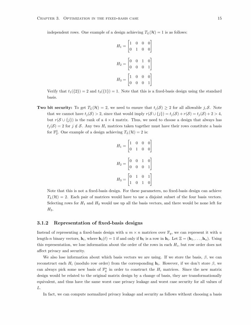
independent rows. One example of a design achieving TL(H) = 1 is as follows:
H1 =
[1 0 0 0
0 1 0 0
]
H2 =
[0 0 1 0
0 0 0 1
]
H3 =
[1 0 0 0
0 0 0 1
]Verify that t1({2}) = 2 and t3({1}) = 1. Note that this is a fixed-basis design using the standard
basis.
Two bit security: To get TL(H) = 2, we need to ensure that tj(S) ≥ 2 for all allowable j,S. Note
that we cannot have tj(S) > 2, since that would imply r(S ∪ {j}) = tj(S) + r(S) = tj(S) + 2 > 4,
but r(S ∪ {j}) is the rank of a 4 × 4 matrix. Thus, we need to choose a design that always has
tj(S) = 2 for j /∈ S. Any two Hi matrices taken together must have their rows constitute a basis
for F42. One example of a design achieving TL(H) = 2 is:
H1 =
[1 0 0 0
0 1 0 0
]
H2 =
[0 0 1 0
0 0 0 1
]
H3 =
[0 1 0 1
1 0 1 0
]Note that this is not a fixed-basis design. For these parameters, no fixed-basis design can achieve
TL(H) = 2. Each pair of matrices would have to use a disjoint subset of the four basis vectors.
Selecting rows for H1 and H2 would use up all the basis vectors, and there would be none left for
H3.
3.1.2 Representation of fixed-basis designs
Instead of representing a fixed-basis design with u m × n matrices over Fq, we can represent it with u
length-n binary vectors, hi, where hi(`) = 1 if and only if b` is a row in hi. Let Ξ = (h1, . . . ,hu). Using
this representation, we lose information about the order of the rows in each Hi, but row order does not
affect privacy and security.
We also lose information about which basis vectors we are using. If we store the basis, β, we can
reconstruct each Hi (modulo row order) from the corresponding hi. However, if we don’t store β, we
can always pick some new basis of Fnq in order to construct the Hi matrices. Since the new matrix
design would be related to the original matrix design by a change of basis, they are transformationally
equivalent, and thus have the same worst case privacy leakage and worst case security for all values of
L.
In fact, we can compute normalized privacy leakage and security as follows without choosing a basis

Chapter 3. Optimization in the fixed-basis case 16
at all.
RL(Ξ) =1
nmax
S⊆{1,...,u}|S|=L
wt
(∨i∈S
hi
)
TL(Ξ) =1
nmin
S⊆{1,...,u}|S|=L
minj /∈S
wt
(hj ∧
∨i∈S
hi
) (3.1)
Recall that wt(·) is the Hamming weight of a vector. We use the symbol∨
to represent the OR
operation and the symbol ∧ to represent the AND operation.
If Ξ is a representation of a fixed-basis design H, then the measures in (3.1) are equivalent to the
definitions of RL(H) and TL(H) given in Definitions 7 and 8. The proof is as follows:
r(S,H) = rank(vsi∈S(Hi))
= size of the largest linearly independent set of rows from all Hi, i ∈ S
= total number of vectors from the basis, β, that are rows in any system in S
= wt
(∨i∈S
hi
)tj(S,H) = r(S ∪ {j},H)− r(S,H)
= wt
(hj ∨
∨i∈S
hi
)− wt
(∨i∈S
hi
)
= wt(hj) + wt
(∨i∈S
hi
)− wt
(hj ∧
∨i∈S
hi
)− wt
(∨i∈S
hi
)
= wt(hj)− wt
(hj ∧
∨i∈S
hi
)
= wt
(hj ∧
∨i∈S
hi
)
3.1.3 Tradeoff by optimization
For fixed-basis designs, we can pose the problem of finding a tradeoff between privacy leakage and
security as an optimization problem over Ξ = (h1, . . . ,hu) as follows:
Problem 1 (Naive optimization). Pick h1, . . . ,hu ∈ {0, 1}n to solve
maximize TL(Ξ),
s.t. RL(Ξ) ≤ R,
wt(hi) = m, i ∈ {1, . . . , u}.
Fix n,m, u, L. Let t∗(R) be the maximum security achieved by Problem 1 for a particular value of
R. We define AFB = {(R, t∗(R))|R ∈ {mn ,m+1n , . . . , n−1n , 1}}.
Proposition 8. Let C be the convex hull of AFB ∪ {(n, 0)}. All achievable normalized privacy-security
pairs for fixed basis designs are contained in C ∩ 1nZ
2.

Chapter 3. Optimization in the fixed-basis case 17
Proof. Let (r, t) be an achievable normalized privacy-security pair for fixed-basis designs. Then there
exists a fixed-basis design Ξ such that (r, t) = (RL(Ξ), TL(Ξ)). By definition of RL(·) and TL(·),(r, t) ∈ 1
nZ2.
Note that r ≤ 1, since RL(·) is measured by taking the Hamming weight of a length n binary vector,
and dividing by n. Also, r ≥ mn , since for any j ∈ S,
wt(∨i∈S
hi) ≥ wt(hj) = m.
Note also that t ≥ 0, since wt(x ∨ y) − wt(x) ≥ 0 for any x,y ∈ Fn2 . Finally, by definition of t∗(·),we must have that t ≤ t∗(r).
3.2 Relaxation
It’s difficult to computationally solve Problem 1 in its current form. For this reason, we relax the
problem, turning it into a linear program (LP).
The relaxation can be thought of as allowing the his to live in the larger space [0, 1]n as opposed to
restricting them to having only binary entries. This is intuitively helpful, however formally we can’t just
add this specification to Problem 1. It would be unclear how to calculate privacy leakage and security
when systems can partially possess rows or basis vectors.
We begin, instead, by defining a relaxed design.
Definition 16. A relaxed design is a vector x = (x1, . . . , x2u) ∈ [0, 1]2u
such that 1Tx = 1.
A relaxed design can be thought of as a concatenation of u subvectors, or ‘blocks’. For k ∈ {0, . . . , u},the kth block has length
(uk
), and each entry in the kth block corresponds to a subset of {1, . . . , u} of
cardinality k. Within the kth block, order the subsets lexicographically. A subset’s corresponding entry
keeps track of the percentage of rows (or basis vectors) that are shared by exactly the systems in that
subset. Let the subset corresponding to x` be denoted P`.An alternative way to think of a relaxed design is as a probability mass function on the power set of
{1, . . . , u}.
Example 3. Let n = 4,m = 2, u = 3. Consider the following fixed-basis matrix design, using the
standard basis, (e1, . . . , en), where each ei has a 1 at the ith coordinate and zeroes elsewhere:
H1 = H2 =
[1 0 0 0
0 1 0 0
], H3 =
[1 0 0 0
0 0 1 0
].
The corresponding relaxed design is x = ( 14 , 0, 0,
14 ,
14 , 0, 0,
14 ). In order to understand why, let’s look first
at the 0th block. x1 = 14 since one out of four basis vectors (e4) isn’t used by any system. In the 1st
block, we have x2 = x3 = 0. This is because there are no basis vectors used only by the first system
or only by the second system. However, x4 = 14 , since there is exactly one vector (e3) which is used
only by the the third system. Similarly, in the 2nd block, x5 = 14 , as exactly one of four basis vectors
(e2) is shared by the first pair of systems, H1 and H2. x6 = x7 = 0 since there is no row vector shared
exclusively by H1 and H3 or by H2 and H3. Finally, in the 3rd block, x8 = 14 , since exactly one of four
basis vectors (e1) is shared by all three systems.

Chapter 3. Optimization in the fixed-basis case 18
We will see that it’s possible to compute privacy leakage and security from a relaxed design. This
should not be surprising, since privacy leakage and security depend solely on the amount of overlap
between systems, and not on the particular rows (or basis vectors) themselves. System overlap is exactly
what is represented by a relaxed design. Thus, we can write down an optimization problem to find the
privacy/security tradeoff, using relaxed designs. It turns out the objective and constraints are all linear
in x, so our problem can be written as a linear program.
Problem 2 (Relaxed LP).
maximize t,
s.t. Tx ≥ t · 1,
Px ≤ R · 1,
x ≥ 0,
1Tx = 1,
Bx = µ · 1.
Recall that we denote the subset corresponding to x` by P`. In Problem 2, B is a u × 2u binary
matrix, with the (i, `)th entry equal to 1 if the ith system belongs to the `th subset P`. Since everything
is normalized by n, for our system size constraint we use µ = mn . P is a
(uL
)×2u binary matrix, with each
row corresponding to some possible leaked subset S with cardinality L, and each column corresponding
to some P`. The (i, `)th entry of P is equal to 1 if the `th subset, P`, includes some system in S. T is a(uL
)· (u−L)× 2u binary matrix with each row corresponding to a unique pair (S, j) of a possible leaked
subset S with cardinality L and a system j /∈ S, and each column corresponding to P`. The (i, `)th
entry of T is equal to 1 if P` includes j but not any system in S.
Example 4. In the case that u = 4 and L = 2, we get the following matrices for B, P , and T :
B =
0 0 0 0 1 0 0 0 1 1 1 0 1 1 1 1
0 0 0 1 0 0 1 1 0 0 1 1 0 1 1 1
0 0 1 0 0 1 0 1 0 1 0 1 1 0 1 1
0 1 0 0 0 1 1 0 1 0 0 1 1 1 0 1
P =
0 1 1 0 0 1 1 1 1 1 0 1 1 1 1 1
0 1 0 1 0 1 1 1 1 0 1 1 1 1 1 1
0 0 1 1 0 1 1 1 0 1 1 1 1 1 1 1
0 1 0 0 1 1 1 0 1 1 1 1 1 1 1 1
0 0 1 0 1 1 0 1 1 1 1 1 1 1 1 1
0 0 0 1 1 0 1 1 1 1 1 1 1 1 1 1
Chapter 3. Optimization in the fixed-basis case 19
T =
0 0 0 0 1 0 0 0 0 0 1 0 0 0 0 0
0 0 0 1 0 0 0 0 0 0 1 0 0 0 0 0
0 0 0 0 1 0 0 0 0 1 0 0 0 0 0 0
0 0 1 0 0 0 0 0 0 1 0 0 0 0 0 0
0 0 0 0 1 0 0 0 1 0 0 0 0 0 0 0
0 1 0 0 0 0 0 0 1 0 0 0 0 0 0 0
0 0 0 1 0 0 0 1 0 0 0 0 0 0 0 0
0 0 1 0 0 0 0 1 0 0 0 0 0 0 0 0
0 0 0 1 0 0 1 0 0 0 0 0 0 0 0 0
0 1 0 0 0 0 1 0 0 0 0 0 0 0 0 0
0 0 1 0 0 1 0 0 0 0 0 0 0 0 0 0
0 1 0 0 0 1 0 0 0 0 0 0 0 0 0 0
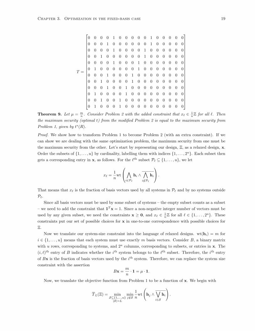
Theorem 9. Let µ = m
n . Consider Problem 2 with the added constraint that x` ∈ 1nZ for all `. Then
the maximum security (optimal t) from the modified Problem 2 is equal to the maximum security from
Problem 1, given by t∗(R).
Proof. We show how to transform Problem 1 to become Problem 2 (with an extra constraint). If we
can show we are dealing with the same optimization problem, the maximum security from one must be
the maximum security from the other. Let’s start by representing our design, Ξ, as a relaxed design, x.
Order the subsets of {1, . . . , u} by cardinality, labelling them with indices {1, . . . , 2u}. Each subset then
gets a corresponding entry in x, as follows. For the `th subset P` ⊆ {1, . . . , u}, we let
x` =1
nwt
∧i∈P`
hi ∧∧i/∈P`
hi
.
That means that x` is the fraction of basis vectors used by all systems in P` and by no systems outside
P`.Since all basis vectors must be used by some subset of systems – the empty subset counts as a subset
– we need to add the constraint that 1Tx = 1. Since a non-negative integer number of vectors must be
used by any given subset, we need the constraints x ≥ 0, and x` ∈ 1nZ for all ` ∈ {1, . . . , 2u}. These
constraints put our set of possible choices for x in one-to-one correspondence with possible choices for
Ξ.
Now we translate our system-size constraint into the language of relaxed designs. wt(hi) = m for
i ∈ {1, . . . , u} means that each system must use exactly m basis vectors. Consider B, a binary matrix
with u rows, corresponding to systems, and 2u columns, corresponding to subsets, or entries in x. The
(i, `)th entry of B indicates whether the ith system belongs to the `th subset. Therefore, the ith entry
of Bx is the fraction of basis vectors used by the ith system. Therefore, we can replace the system size
constraint with the assertion
Bx =m
n· 1 = µ · 1.
Now, we translate the objective function from Problem 1 to be a function of x. We begin with
TL(Ξ) = minS⊆{1,...,u}|S|=L
minj /∈S
1
nwt
(hj ∧
∨i∈S
hi
).

Chapter 3. Optimization in the fixed-basis case 20
Maximizing TL(Ξ) is equivalent to maximizing some variable t such that 1nwt
(hj ∧
∨i∈S hi
)≥ t for all
eligible pairs (S, j). Note that wt(hj ∧
∨i∈S hi
)is the number of basis vectors used by the jth system
but not by any system in S. Consider T , a binary matrix with(uL
)· (u−L) rows, corresponding to pairs
of cardinality-L subsets S and systems j not in those subsets, and 2u columns, corresponding to subsets
P`, or entries of x. The (i, `)th entry of T indicates whether P` includes j but not any system in S.
Therefore, the ith entry of Tx is equal to 1n tj(S). Thus, we get the constraint
Tx ≥ t · 1
Our objective is to maximize t.
Finally, we translate the privacy leakage constraint to be in terms of x. We begin with
RL(Ξ) = maxS⊆{1,...,u}|S|=L
1
nwt
(∨i∈S
hi
).
Note that wt(∨
i∈S hi)
is the number of vectors used by some system in S. Consider P , a binary matrix
with(uL
)rows, corresponding to leaked subsets S of cardinality L, and 2u columns, corresponding to
subsets P`, or entries in x. The (i, `)th entry of P indicates whether the `th subset, P`, includes some
system in S, i.e., whether S ∩ P` is nonempty. Thus, the ith entry of Px is equal to 1nr(S). Requiring
RL(Ξ) ≤ R is equivalent to requiring 1nr(S) ≤ R for all S ⊆ {1, . . . , u} of cardinality L. Therefore we
get the constraint
Px ≤ R · 1.
Note 5. Without the x` ∈ 1nZ restriction, Problem 2 provides an upper bound on Problem 1 for all n,
since Problem 2 searches for designs over a larger feasible set.
Lemma 10. Let x∗ be an optimal solution to Problem 2. Let F be the set of feasible solutions to Problem
2. We can find a vector x ∈ F with rational entries which is arbitrarily close in norm to x∗.
Proof. F is the intersection of an affine subspace and a number of half-spaces. The affine subspace is
characterized by linear equations with rational coefficients. Thus, it is spanned by rational vectors. Any
point p ∈ F can therefore be written as a linear combination of rational vectors with real coefficients.
Each of these real coefficients can be arbitrarily closely approximated by a rational number, creating a
new linear combination p in the affine subspace which can be made arbitrarily close to p. Therefore,
rational vectors are dense in the affine subspace. Take a ball around x∗ which is open with respect to
the subspace and intersect it with the open half-spaces of F . The resulting set is open, and therefore
contains rational vectors, since rational vectors are dense in the affine subspace.
Corollary 11. As n gets large, the maximum security from Problem 1 approaches the maximum security
from Problem 2.
Proof. Let x∗ be an optimal solution to Problem 2. Take x as given in Lemma 10. We know that for
some large enough n, x must be a feasible solution to Problem 2 with the added restriction that x` ∈ 1nZ.
Since the objective function of an LP is continuous in the LP’s variables, we have that the difference

Chapter 3. Optimization in the fixed-basis case 21
between the maximum security in the two LPs can be made arbitrarily small. Due to Theorem 9, we
have that the maximum security in Problem 1 is equal to the maximum security in Problem 2 with the
added constraint.
3.3 Simplification
In this section, we simplify Problem 2 so it’s no longer prohibitively computationally intensive to execute
as an LP.
3.3.1 Variable reduction
Recall that we divided a relaxed design into blocks of length(uk
).
Definition 17. A relaxed design is block-constant if within the kth block, all entries are equal. That is,
a block-constant x has the form
x = (y0, y1, . . . , y1, y2, . . . , y2, . . . , yu−1, . . . , yu−1, yu),
where yk is repeated(uk
)times.
Theorem 12. Problem 2 admits a block-constant solution.
Proof. Take any optimal solution, given by
x = (x1, x2, . . . , x2u),
achieving cost t∗. We will see that relabelling the u systems induces another solution, x, which is a
permutation of x. This solution is feasible, because the constraints on each system are the same. This
solution is also optimal, achieving cost t∗, due to the symmetry of the objective function. Due to the
convexity of LPs, any convex combination of x and x is also a feasible solution, and due to linearity of
the objective function, also achieves cost t∗.
With this construction in mind, we generate u! (not necessarily unique) solutions as follows. We first
generate all possible relabellings of the u systems. Each relabelling corresponds to some π ∈ Su, the
symmetric group of permutations of u objects.
Now we will see how a permutation π ∈ Su, used to relabel the systems, corresponds to a permutation
γ ∈ S2u , which reorders entries of x. Let the matrix B be a u × 2u binary matrix, with each length
u binary vector occupying one column in such a way that the columns are arranged from left to right
in order of ascending Hamming weight. The ith row corresponds to the ith system, and the jth column
corresponds to the jth subinterval of the unit interval, with length given by xj . Bij = 1 indicates that the
ith system occupies the jth portion of the unit interval. Relabelling the u systems therefore corresponds
to a reordering of the rows of B, producing a new matrix PπB (where Pπ is the permutation matrix
implementing π). Note that when the rows are reordered, this does not affect the weight of each column.
Also, note that each column in PπB is unique, because the columns of B are unique, and permutations
within the column vectors are bijections. Therefore, the columns of PπB are simply the columns of B
rearranged, still ordered by Hamming weight.

Chapter 3. Optimization in the fixed-basis case 22
The induced column permutation only acts within blocks of fixed column weight. Thus,
PπB = BPγ ,
where γ is the induced column permutation, and where Pγ has a block-diagonal form with the kth block
being a permutation matrix on(uk
)elements. We have defined a map φ : Su → S2u .
Additionally, this map is injective. Let π1, π2 ∈ Su such that φ(π1) = φ(π2) = γ. Then Pπ1B = Pπ2B.
Since permutation matrices are invertible, we have that B = P−1π1Pπ2B. However, the composition of
permutations is a permutation, and since the rows of B are distinct, it must be the identity, i.e. P−1π1Pπ2 =
I. Thus, Pπ1 = (P−1π1)−1 = Pπ2 , so π1 = π2. We have that φ is injective, and |φ(Su)| = |Su| = u!.
It is now easy to see that φ is a group antihomomorphism from Su to a subgroup of S2u , i.e.
that φ(π1 ◦ π2) = φ(π2) ◦ φ(π1) for all π1, π2 ∈ Su. Here, the ◦ operation represents composition of
permutations. This is because if φ(πi) = γi, i = 1, 2, then
Pπ1◦π2B = Pπ1Pπ2B = Pπ1BPγ2 = BPγ2Pγ1 = BPγ2◦γ1 .
Therefore, G = (φ(Su), ◦) is a subgroup of (S2u , ◦).
Now let J = {1, . . . , 2u}. Define a group action, ∗ : G× J → J , of G on J as follows. A permutation
γ ∈ G maps each index in J to some other index in J . Essentially, if we think of permutations as vectors,
γ ∗ j selects the jth element of γ. Fix `, j ∈ J , such that columns ` and j in B have the same Hamming
weight, k. Let γ ∈ G such that γ ∗ ` = j. Let
Stab(j) = {κ ∈ G : κ ∗ j = j}.
|Stab(j)| = (u − k)!k!, because there are u − k zeros and k ones to rearrange within the column while
still mapping j to itself. However, we know that the set of permutations in G mapping ` to j is exactly
the set γ ◦ Stab(j), thus by injectivity of γ, there are exactly (u− k)!k! permutations in G mapping ` to
j.
Thus, if we use all u! orderings of the systems (rows) to induce u! permutations of the columns, and
then average the permutations of x to obtain x, we get that for any j corresponding to a column with
weight k,
xj =1
u!
∑` with weight k
(u− k)!k!x` =1(uk
) ∑` with weight k
x`.
Thus, all entries within a block of fixed weight will take on the same value, obtained by averaging the
original entries of that block.
By the arguments made at the beginning of the proof, (i.e. due to convexity and linearity,) x
will be feasible and optimal, achieving cost t∗. Therefore, Problem 2 admits a block-constant optimal
solution.

Chapter 3. Optimization in the fixed-basis case 23
Now consider the following LP.
Problem 3 (LP: Reduced variables).
maximize t,
s.t. TAy ≥ t · 1,
PAy ≤ R · 1,
y ≥ 0,
1TAy = 1,
BAy = µ · 1.
In this LP, A is the 2u × (u+ 1) matrix describing the linear map that takes y ∈ Ru+1 to x, such that
xj = yk, where k is the cardinality of the subset corresponding to xj , i.e., | ∓j | = k.
Example 5. When u = 4, as in Example 4, we have that
AT =
1 0 0 0 0 0 0 0 0 0 0 0 0 0 0 0
0 1 1 1 1 0 0 0 0 0 0 0 0 0 0 0
0 0 0 0 0 1 1 1 1 1 1 0 0 0 0 0
0 0 0 0 0 0 0 0 0 0 0 1 1 1 1 0
0 0 0 0 0 0 0 0 0 0 0 0 0 0 0 1
Theorem 13. Problem 2 and Problem 3 are equivalent.
Proof. Because of Theorem 12, we can let x∗ be a block-constant solution to Problem 2. Let y∗k denote
the value shared by all entries in the kth block of x∗. Let y∗ = (y∗0 , . . . , y∗u)T . Note that we can write
x∗ = Ay∗, where A is as in Problem 3. Thus, we have that Ay∗ is an optimal solution to Problem 2.
Equivalently, y∗ is an optimal solution to Problem 3. The optimal security in Problem 2 is Tx∗ which
is equal to the optimal security in Problem 3, given by TAy∗.
3.3.2 Constraint reduction
Consider the following LP:
Problem 4 (LP: Reduced constraints).
maximize gTy,
s.t. cTy ≤ R,
y ≥ 0,
fTu y = 1,
[0 fTu−1]y = µ,
where g = [0 fTu−L−1 0T ]T , fn = ((n0
),(n1
),(n2
), . . . ,
(nn
))T , and c = (c0, . . . , cu)T , with
ci =
(ui
)−(u−Li
), i ≤ u− L,(
ui
), i > u− L.

Chapter 3. Optimization in the fixed-basis case 24
Lemma 14. Let i ∈ {0, . . . , u}. Let k− = max(1, i− (u− L)) and k+ = min(L, i). Then
k+∑k=k−
(L
k
)(u− Li− k
)=
(ui
)−(u−Li
), i ≤ u− L,(
ui
), i > u− L.
Proof. There are two cases. First, consider the case where i ≤ u− L. Note that k− = 1. If i < L, then
k+ = i, and
ci =
[i∑
k=0
(L
k
)(u− Li− k
)]−(L
0
)(u− Li
)=
(u
i
)−(u− Li
).
If i ≥ L, then k+ = L, and
ci =
L∑k=0
[(L
k
)(u− Li− k
)]−(L
0
)(u− Li
)=
(u
i
)−(u− Li
).
Now, consider the case where i > u− L. Note that k− = i− (u− L). If i < L, then k+ = i, and
ci =
[i∑
k=0
(L
k
)(u− Li− k
)]−
i−(u−L)−1∑k=0
(L
k
)(u− Li− k
)=
(u
i
)−
i∑j=u−L+1
(L
i− j
)(u− Lj
) =
(u
i
)− 0 =
(u
i
),
since(u−Lj
)is defined as 0 for j > u− L. Finally, if i ≥ L, then k+ = L, and
ci =
L∑k=i−(u−L)
(L
k
)(u− Li− k
)=
u−i∑j=0
(L
L− j
)(u− L
i− L+ j
)
=
u−i∑j=0
(L
j
)(u− L
(u− i)− j
)=
(u
u− i
)=
(u
i
).
Theorem 15. Problem 3 and Problem 4 are equivalent.
Proof. There are four parts to this proof. Each part corresponds to a different pair of constraints from
the two LPs.
1. Security
In Problem 3, the security constraint is TAy ≥ t · 1. We will see that each row of TA is equal
to gT . Take an arbitrary row of TA, and denote it (t0, . . . , tu). Recall that for some set S of L
systems and some j /∈ S, the corresponding row of T indicates which intervals are members of {j}but not of any system in S. For i ∈ {0, . . . , u}, ti is the inner product of our selected row of T
with the ith column of A. In the ith column of A, the entries with value 1 correspond exactly to
the intervals occupied by precisely i systems. Thus, ti is the number of intervals occupied by the
jth system, but not by any system in S, that are shared by exactly i systems. In other words, ti
counts how many intervals are shared by the jth system and i − 1 other systems, none of which
are in S.

Chapter 3. Optimization in the fixed-basis case 25
It is clear that t0 = 0. For 1 ≤ i ≤ u − L, ti =(u−L−1i−1
), which is the number of ways to choose
the i− 1 other systems from among the u− L− 1 systems which are not j and are not in S. For
i > u− L, there aren’t enough systems outside of S to choose from, so in that case ti = 0.
Thus, each row of TA is equal to gT , so the vector constraint TAy ≥ t ·1 is just (u−L)(uL
)copies
of the scalar constraint gTy ≥ t. The objective in Problem 3 is to maximize t as long as it is no
greater than gTy, which is equivalent to just maximizing gTy, since t appears nowhere else. Thus,
the t is dropped in Problem 4 for simplicity.
2. Privacy leakage
In Problem 3, the privacy leakage constraint is PAy ≤ R · 1. We will see that each row of PA is
equal to cT . Take an arbitrary row of PA, and denote it (p0, . . . , pu). Recall that for some set Sof L systems, the corresponding row of P indicates which intervals are members of systems in S.
For i ∈ {0, . . . , u}, pi is the inner product of our selected row of P with the ith column of A. In the
ith column of A, the entries with value 1 correspond exactly to the intervals occupied by precisely
i systems. Thus, pi is the number of intervals occupied by systems in (S), which are shared by
exactly i systems. In other words, pi counts how many intervals are shared by k systems from Sand i−k systems outside S, for any k for which that breakdown is possible. For a particular value
of k, there are(Lk
)ways to choose systems from S and
(u−Li−k)
ways to choose systems outside S.
Thus, pi =∑k
(Lk
)(u−Li−k), for admissible values of k.
The number of systems chosen from S must obviously be no greater than L, and must also be no
greater than i, because our aim is to choose i systems in total. Formally,
k ≤ min(i, L).
Similarly, the number of systems chosen from outside S must be no greater than u−L. Finally, we
must choose at least one system from S, due to the nature of P . Thus, we must choose no more
than i− 1 systems from outside S. Formally, i− k ≤ min(i− 1, u− L). Equivalently,
k ≥ max(1, i− (u− L)).
Therefore, by Lemma 14, pi = ci, and the vector constraint PAy ≤ R · 1 is just(uL
)copies of the
scalar constraint cTy ≤ R.
3. Interval lengths sum to one
In Problem 3, we have the equality constraint 1TAy = 1. Let 1TA be denoted (a0, . . . , au). For
i ∈ {0, . . . , u}, ai is the sum of the elements in the ith column of A, which contains a 1 for each
interval that is shared by exactly i systems. There are(ui
)ways to pick i systems, and since all
possible combinations exist, ai =(ui
). Thus, 1TA = fTu .
4. Fixed system size
In Problem 3, the system size constraint is BAy = µ · 1. We will see that each row of BA is equal
to [0 fTu−1]. Take an arbitrary row of BA, and denote it (b0, . . . , bu). Recall that each row of B
corresponds to a particular system, indicating which intervals are members of that system. For
i ∈ {0, . . . , u}, bi is the inner product of our selected row of B with the ith column of A. Thus, bi
is the number of intervals occupied by our system and exactly i− 1 other systems.

Chapter 3. Optimization in the fixed-basis case 26
It is clear that b0 = 0. For i > 0, bi =(u−1i−1), which is the number of ways to choose i − 1 other
systems to share an interval with from among the u− 1 other systems.
Thus, each row of BA is equal to [0 fTu−1], so the vector constraint BAy = µ · 1 is just u copies of
the scalar constraint [0 fTu−1]y = µ.
We began with a discrete optimization problem (Problem 1) and relaxed it to form an LP (Problem
2) which gives an outer bound on the region of achievable privacy-security pairs. For large n, that bound
is very tight. We then reduced the number of variables in Problem 2 to produce Problem 3. We did
this by forcing solutions to be block-constant, and proved that this does not decrease optimal security.
Finally, we found many of the constraints in Problem 3 to be redundant and removed them, leaving us
with Problem 4.
Proposition 16. Problem 4 is feasible for 1 ≤ L < u, µ ∈ [0, 1], and R ≥ µ.
Proof. Let R ≥ µ. Consider the solution y = (1 − µ, 0, 0, . . . , 0, µ). For the first inequality constraint,
we have cTy = 0 · (1 − µ) + 1 · µ = µ ≤ R which holds by assumption. The constraint y ≥ 0 clearly
holds. For the first equality constraint, we have fTu y = 1 · (1 − µ) + 1 · µ = 1. For the second equality
constraint, we have [0 fTu−1]y = 0 · (1− µ) + 1 · µ = µ. Therefore, y is a feasible solution, so Problem 4
is feasible.
Theorem 17. A solution to Problem 4, denoted y∗, has at most three nonzero entries.
Proof. If u < 3, the result is trivial. Thus, let u ≥ 3. Let y(0) = y∗ be a solution to Problem 4. Let
R∗ = cTy∗.
We know that y(0) also solves the following LP, denoted P (0):
maximize gTy,
s.t. cTy = R∗,
y ≥ 0,
fTu y = 1,
[0 fTu−1]y = µ,
The feasible set for P (0) is given by an affine subspace, F (0), intersecting the positive orthant,
y ≥ 0. Since there are 3 affine equality constraints, we know that the dimension of F (0) is at least
u + 1 − 3 = u − 2 ≥ 1. Since we have a linear objective, y(0) must be on the boundary of F (0), i.e., it
must have an entry equal to zero. Let i(0) be the index of that entry.
Remove the i(0)th coordinate from every vector in P (0) to generate P (1). Let y(1) be y(0) with the
i(0)th coordinate removed. P (1) is an optimization over real vectors of length u. Note that y(1) solves
P (1).
Let F (1) be the affine subspace from P (1). Again, we have an LP with 3 affine equality constraints,
so the dimension of F (1) is at least u− 3. If u− 3 ≥ 1, we can again find an entry of y(1) which is equal
to zero, because y(1) must be on the boundary of F (1). Let i(1) be the index of that entry.
Chapter 3. Optimization in the fixed-basis case 27
This process will continue to iterate, by continuing to remove coordinate i(k−1) to construct P (k),
an LP with u + 1 − k variables. Each iteration, y(k) will be a solution to P (k). Recall that y(k) is a
subvector of y∗. On the kth iteration, the dimension of the feasible set will be u− 2− k.
While u− 2− k ≥ 1 (i.e., k ≤ u− 3), we can find a new entry of y∗ which must be zero. That means
there must be at least u−3 entries of y∗ which are zero. When k = u−2, F (u−2) is zero-dimensional, i.e.,
is just a point, and therefore does not necessarily intersect any coordinate axis. That is to say, P (u−2)
only has one feasible solution, and there is no guarantee that the solution contains any zero entries.
3.4 The privacy-security tradeoff
In this section, we examine the tradeoff between privacy leakage and security when working in the
fixed-basis design space.
0.5 0.55 0.6 0.65 0.7 0.75 0.8 0.85 0.9 0.95 10
0.05
0.1
0.15
0.2
0.25
Normalized privacy leakage
Nor
mal
ized
sec
urity
L=1L=2L=3L=4L=5L=6L=7L=8L=9
Figure 3.1: The area under each curve is the region of achievable privacy-security pairs for fixed-basisdesigns with u = 10 and µ = 0.5. The curves were generated by running the LP of Problem 4 for valuesof R between µ and 1.
Problem 4 was implemented in MATLAB, and then run for various values of µ, u, L. For each choice of
those values, R was incremented in small steps between µ and 1, and the LP was run for each value of R.
Maximum security values were then plotted vs. R, indicating the optimal performance of relaxed designs,
as can be seen in Figure 3.1. There are more examples in the appendix. These curves provide an outer
bound on the region of achievable privacy-security pairs, (RL(Ξ), TL(Ξ)), for fixed-basis designs. Recall,
however, that any point on these tradeoff curves is arbitrarily close to an achievable privacy-security
pair, corresponding to an actual fixed-basis design for some value of n which is large enough.

Chapter 3. Optimization in the fixed-basis case 28
Note that the normalized privacy leakage axis begins at µ. This is because at least one system is
leaked in all cases, and the normalized privacy leakage associated with one system is equal to µ = mn .
This also explains why for any choices of µ and u, the L = 1 curve is constant.
It should also be noted that beyond some value of R, there is no longer any increase in security.
This happens when an upper bound on privacy leakage becomes a looser constraint than trying to fit
u k-dimensional subspaces into an n dimensional space while overlapping as little as possible. At that
point, the privacy-security tradeoff curves flatten out.
At first, as L increases, the maximum achievable security (at R = 1) decreases, i.e., the curves flatten
out at smaller and smaller security values. Then, beyond some value of L, the curves all approach the
same level. This is because when privacy leakage is no longer a constraint, our goal is to spread the
systems as far apart as possible. The final level has to do with how many disjoint subsets of size L can
be selected from u sets. As L approaches u, this number stops decreasing and just hits 1.
Finally, note that as the number of leaked systems is increased, the achievable privacy-security pairs
occupy a decreasing sequence of regions, each contained in the one before it.
3.4.1 A form for optimal solutions
When looking at the vectors y∗ solving Problem 4, an interesting pattern in the solutions is apparent.
This section focuses on describing this pattern.
Let K0 = bµuc. Let K1 = d uL − 1e. Let K = min{K0,K1}. For k ∈ {0, . . . ,K}, let
αk = (1− µ)
(u−Lk
)(u−1k
) . (3.2)
Conjecture 18. Let k ∈ {0, . . . ,K − 1}. Let R ∈ [1−αk, 1−αk+1). Then Problem 4 admits a solution
y∗ = (y∗0 , . . . , y∗u)T with y∗i = 0 for all i /∈ {k, k + 1, u}. Alternatively, if R ≥ 1− αK , Problem 4 admits
a solution with y∗i = 0 for all i /∈ {K,K + 1, u}.
We now introduce an LP that is equivalent to Problem 4 if Conjecture 18 holds. Problem 5 is
obtained by taking Problem 4, and forcing the appropriate yi = 0 as indicated by the conjecture.
Problem 5 (LP: Three variables). If µ ≤ R < 1 − αK , let k ∈ {0, . . . ,K − 1} be such that R ∈[1− αk, 1− αk+1). Else, if R ≥ 1− αK , let k = K.
maximize gkyk + gk+1yk+1,
s.t. ckyk + ck+1yk+1 + yu ≤ R,
yk ≥ 0,
yk+1 ≥ 0,
yu ≥ 0,(u
k
)yk +
(u
k + 1
)yk+1 + yu = 1,(
u− 1
k − 1
)yk +
(u− 1
k
)yk+1 + yu = µ.

Chapter 3. Optimization in the fixed-basis case 29
Proposition 19. Problem 5 is solved by the optimal y∗k from Problem 6. In Problem 5,
y∗k+1 =k + 1
u− k − 1
(1− µ(u−1k
) − y∗k),
y∗u =1
u− k − 1
(y∗k
(u
k
)+ µu− k − 1
).
(3.3)
Proof. From the two equality constraints in Problem 5, we can solve analytically for yk+1 and yu in
terms of yk. The solutions are given in (3.3).
This means the positivity constraints from Problem 5 can be rewritten as
yk ≥ 0,
yk ≤1− µ(u−1k
) ,yk ≥
k + 1− µu(uk
) .
We now show that for k < K1, k + 1 ≤ u− L. We have that
k + 1 ≤ K1 =⌈ uL− 1⌉
=
⌈u− LL
⌉≤ u− L.
Thus, we have gk =(u−L−1k−1
), ck =
(uk
)−(u−Lk
)and for k < K1, gk+1 =
(u−L−1
k
)and ck+1 =(
uk+1
)−(u−Lk+1
).
For k < K1, the objective function becomes
(u− L− 1
k − 1
)yk +
(u−L−1
k
)(k + 1)
u− k − 1
(1− µ(u−1k
) − yk)
=
(u− L− 1
k
)(k
u− L− k− k + 1
u− k − 1
)yk +
(u−L−1
k
)(k + 1)(1− µ)(
u−1k
)(u− k − 1)
=
(u− L− 1
k
)(L(k + 1)− u
(u− L− k)(u− k − 1)
)yk +
(u−L−1
k
)(k + 1)(1− µ)(
u−1k
)(u− k − 1)
Maximizing this is equivalent to maximizing (L(k + 1) − u)yk. We leave off the constant term when
writing Problem 6 for simplicity.
For k < K1, the privacy leakage constraint becomes
((u
k
)−(u− Lk
))yk +
((uk+1
)−(u−Lk+1
))(k + 1)
u− k − 1
(1− µ(u−1k
) − yk)+yk(uk
)+ µu− k − 1
u− k − 1≤ R
⇔[(u− k − 1)
((u
k
)−(u− Lk
))+ (k + 1)
((u− Lk + 1
)−(
u
k + 1
))+
(u
k
)]yk
≤ R(u− k − 1)−(1− µ)
((uk+1
)−(u−Lk+1
))(k + 1)(
u−1k
) − µu+ k + 1

Chapter 3. Optimization in the fixed-basis case 30
⇔−(u− Lk
)(L− 1)yk
≤ −(1−R)(u− k − 1) +(1− µ)(u−1k
) [u(u− 1
k
)− (k + 1)
(u
k + 1
)+ (k + 1)
(u− Lk + 1
)]⇔(u− Lk
)(L− 1)yk ≥ (1−R)(u− k − 1)−
(1− µ)(u−Lk
)(u− L− k)(
u−1k
) .
When L > 1, the above is equivalent to
yk ≥(1−R)(u− 1− k)
(L− 1)(u−Lk
) − (1− µ)(u− L− k)
(L− 1)(u−1k
) .
When L = 1, the privacy leakage constraint just becomes (1 − R)(u − k − 1) ≤ (1 − µ)(u − k − 1), or
equivalently, R ≥ µ.
In Problem 5, in the case that k = K1, there are two possibilities for how the objective function and
privacy leakage constraint will look. Either K1 + 1 ≤ u− L, so the above analysis for k < K also holds
for k = K1.
Else, if K1 + 1 > u−L, then gk+1 = 0, so we just want to maximize any positive constant multiplied
by yk. This means we want to send yk to its upper bound, so the privacy leakage constraint, lower-
bounding yk, is irrelevant. We have (K1 + 1)L − u ≥ 0, so the objective in Problem 6 indeed has a
positive coefficient.
Putting all of this together gives us Problem 6, with a shifted objective function.
Problem 6 (LP: One variable). If L ≥ 2, we have the following LP, with R ∈ [1 − αk, 1 − αk+1), or
R ≥ 1− αK and k = K. If L = 1, replace the last constraint with R ≥ µ.
maximize ((k + 1)L− u)yk,
s.t. yk ≤1− µ(u−1k
) ,yk ≥ 0,
yk ≥k + 1− µu(
uk
) ,
yk ≥(1−R)(u− 1− k)
(L− 1)(u−Lk
) − (1− µ)(u− L− k)
(L− 1)(u−1k
) .
3.4.2 Expressions for the tradeoff
Now that we have an LP in one variable, we no longer need to solve it computationally.
Before we solve it analytically, we need to prove a preliminary result. Let
R0 = 1− αK0
1− µ
((1− µL) +
K0(L− 1)
u
).
Lemma 20. R0 ≥ 1− αK .
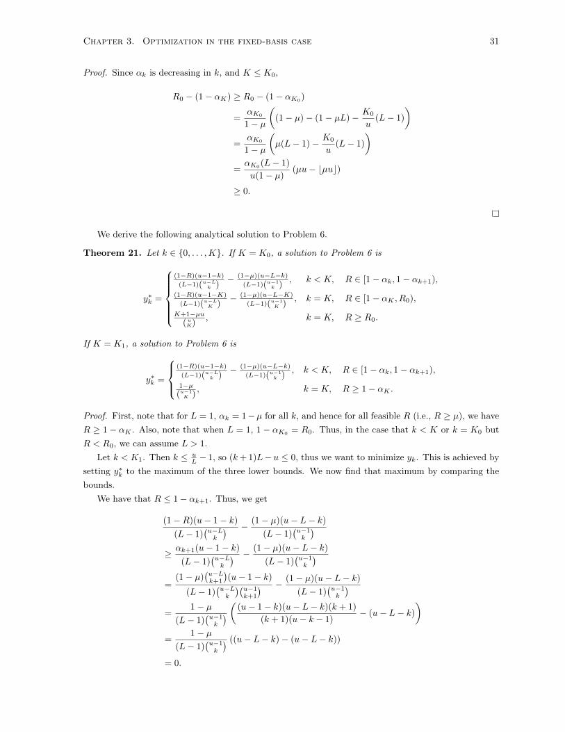
Chapter 3. Optimization in the fixed-basis case 31
Proof. Since αk is decreasing in k, and K ≤ K0,
R0 − (1− αK) ≥ R0 − (1− αK0)
=αK0
1− µ
((1− µ)− (1− µL)− K0
u(L− 1)
)=
αK0
1− µ
(µ(L− 1)− K0
u(L− 1)
)=αK0(L− 1)
u(1− µ)(µu− bµuc)
≥ 0.
We derive the following analytical solution to Problem 6.
Theorem 21. Let k ∈ {0, . . . ,K}. If K = K0, a solution to Problem 6 is
y∗k =
(1−R)(u−1−k)(L−1)(u−L
k )− (1−µ)(u−L−k)
(L−1)(u−1k )
, k < K, R ∈ [1− αk, 1− αk+1),
(1−R)(u−1−K)
(L−1)(u−LK )
− (1−µ)(u−L−K)
(L−1)(u−1K )
, k = K, R ∈ [1− αK , R0),
K+1−µu(uK)
, k = K, R ≥ R0.
If K = K1, a solution to Problem 6 is
y∗k =
(1−R)(u−1−k)(L−1)(u−L
k )− (1−µ)(u−L−k)
(L−1)(u−1k )
, k < K, R ∈ [1− αk, 1− αk+1),
1−µ(u−1
K ), k = K, R ≥ 1− αK .
Proof. First, note that for L = 1, αk = 1−µ for all k, and hence for all feasible R (i.e., R ≥ µ), we have
R ≥ 1− αK . Also, note that when L = 1, 1− αK0 = R0. Thus, in the case that k < K or k = K0 but
R < R0, we can assume L > 1.
Let k < K1. Then k ≤ uL − 1, so (k+ 1)L− u ≤ 0, thus we want to minimize yk. This is achieved by
setting y∗k to the maximum of the three lower bounds. We now find that maximum by comparing the
bounds.
We have that R ≤ 1− αk+1. Thus, we get
(1−R)(u− 1− k)
(L− 1)(u−Lk
) − (1− µ)(u− L− k)
(L− 1)(u−1k
)≥ αk+1(u− 1− k)
(L− 1)(u−Lk
) − (1− µ)(u− L− k)
(L− 1)(u−1k
)=
(1− µ)(u−Lk+1
)(u− 1− k)
(L− 1)(u−Lk
)(u−1k+1
) − (1− µ)(u− L− k)
(L− 1)(u−1k
)=
1− µ(L− 1)
(u−1k
) ( (u− 1− k)(u− L− k)(k + 1)
(k + 1)(u− k − 1)− (u− L− k)
)=
1− µ(L− 1)
(u−1k
) ((u− L− k)− (u− L− k))
= 0.

Chapter 3. Optimization in the fixed-basis case 32
We have just seen that 0 is not the maximum lower bound. Now we need to compare the other two
lower bounds on yk. We do this by comparing the following expression to 0:
(1−R)(u− 1− k)
(L− 1)(u−Lk
) − (1− µ)(u− L− k)
(L− 1)(u−1k
) − k + 1− µu(uk
) . (3.4)
To simplify the comparison, we note that L− 1 = (u− 1− k)− (u− L− k), and multiply (3.4) by the
positive quantity (L− 1)(u− k)(u−Lk
)(uk
), to get
(1−R)(u− 1− k)(u− k)
(u
k
)− (1− µ)(u− L− k)u
(u− Lk
)− [(1− µ)u− (u− 1− k)]
(u− Lk
)(u− k)[(u− 1− k)− (u− L− k)]
(3.5)
We then further simplify the expression from (3.5) to obtain:
(1−R)(u− 1− k)(u− k)
(u
k
)− (1− µ)uL(u− 1− k)
(u− Lk
)+ (L− 1)
(u− Lk
)(u− k)(u− k − 1).
(3.6)
Note that for k < K, R < 1− αK . Hence, by Lemma 20, R < R0.
Thus, (3.6) is greater than
(1−R0)(u− 1− k)(u− k)
(u
k
)− (1− µ)uL(u− 1− k)
(u− Lk
)+ (L− 1)
(u− Lk
)(u− k)(u− k − 1)
=αK0
1− µ
((1− µL) +
K0(L− 1)
u
)(u− 1− k)(u− k)
(u
k
)− (1− µ)uL(u− 1− k)
(u− Lk
)+ (L− 1)
(u− Lk
)(u− k)(u− k − 1)
=
(u− Lk
)(u− 1− k) (u(1− µL) +K0(L− 1)− uL(1− µ) + (L− 1)(u− k))
=
(u− Lk
)(u− 1− k)(K0 − k)(L− 1)
(3.7)
Since k < K ≤ K0, (3.7) is positive. Therefore, (3.4) is greater than 0, so we have that for k < K,
y∗k = (1−R)(u−1−k)(L−1)(u−L
k )− (1−µ)(u−L−k)
(L−1)(u−1k )
.
Now let’s examine the case that k = K = K0. We want to minimize yk, since k < K1. Again, we
need to find the maximum of the three lower bounds. If R < R0, we still have that (3.4) is greater than
0, by the above arguments. Also, we have that
K0 + 1− µu(uK0
) =1− (µu− bµuc)(
uK0
) ≥ 0.
Thus, the maximal lower bound is the same one as when k < K, so the expression for y∗k is also the
same.
However, if R ≥ R0, we have that the expression in (3.6) is less than or equal to the expressions in

Chapter 3. Optimization in the fixed-basis case 33
(3.7). Further, since k = K0, the last line of (3.7) is just 0. Thus, in that case, the maximum of the
three lower bounds (and hence y∗k) isK0 + 1− µu(
uK0
) .
Finally, in the case that k = K1, then (k + 1)L − u ≥ 0, so we want to maximize yk. In that case,
there is only one upper bound, so y∗k = 1−µ(u−1
K1).
Theorem 22. Let k ∈ {0, . . . ,K}. Let R ≥ µ. The maximal security level (for relaxed designs)
achievable in Problem 5 is given by:
t∗ =
αk(u−L−k)−(1−R)(u−L−kL)(u−L)(L−1) , k < K, R ∈ [1− αk, 1− αk+1),
αK0(u−L−K0)−(1−R)(u−L−K0L)
(u−L)(L−1) , k = K0, R ∈ [1− αK0, R0),
αK0(µu(u−L−K0)+K0L(1−(µu−K0)))
(1−µ)u(u−L) , k = K0, R ≥ R0,K1αK1
u−L , k = K1, R ≥ 1− αK1.
Proof. This result follows from combining the results in Proposition 19 and Theorem 21, and then
plugging y∗k, y∗k+1, and y∗u into the objective function from Problem 5.
For each k ∈ {0, . . . ,K}, for R = 1−αk and for R = R0, we have plotted the analytical security levels
predicted in Theorem 22, for various values of µ, u, L, and superimposed them on the optimization results
of Problem 4. The results can be seen in Figure 3.2, as well as in the appendix. The perfect coincidence
of the analytical expressions and the optimization plots indicate the likely truth of Conjecture 18.
0.5 0.55 0.6 0.65 0.7 0.75 0.8 0.85 0.9 0.95 10
0.05
0.1
0.15
0.2
0.25
Normalized privacy leakage
Nor
mal
ized
sec
urity
L=1L=2L=3L=4L=5L=6L=7L=8L=9
Figure 3.2: This is Figure 3.1, with the analytic predictions of Theorem 22 superimposed for u = 10,µ = 0.5. Note that the predicted points align exactly with the optimization results.

Chapter 4
Conclusions
4.1 Summary of results
First, the problem of designing multiple secure-sketch biometric authentication systems with low worst-
case privacy leakage and high worst-case security was introduced. This was shown to be equivalent to
a problem of subgraph selection on the subspace Hasse diagram. Equivalence classes of designs were
introduced. Transformational equivalence and graphical equivalence were found to be the same, and
both were found to imply performance equivalence.
Fixed-basis designs were then introduced, along with a simpler representation for designs. A linear
program was constructed which can generate the privacy-security tradeoff for fixed-basis designs. The
linear program was reduced to one with many fewer variables and constraints.
It was proven that at most three of the variables in the optimal solution are non-zero. A conjecture
was made regarding which variables these are. Assuming the truth of the conjecture, an analytical
expression for the tradeoff was discovered which matched the optimization results.
4.2 Directions for future work
The most obvious direction for further work is to prove Conjecture 18. Doing that would verify our
analytical expression for the privacy-security tradeoff in the fixed-basis case.
Another interesting direction is to determine how to use the optimization results to construct real
fixed-basis designs with good performance. It seems like a simple task at first, just rounding the entries
of y∗ to be multiples of 1n and then working backwards from that relaxed design to get a fixed-basis
design. The difficulty is that once rounding is performed, the resultant vector may no longer be in the
subspace of Ru+1 defined by the equality constraints in Problem 4. Thus, there needs to be a way to find
a relaxed design close to the optimal y∗ that has entries in 1nZ, such that the design itself is contained
in the requisite u− 1 dimensional subspace.
Just as it was possible to relax the fixed-basis design problem to find the privacy-security tradeoff
for fixed-basis designs, it may also be possible to relax the general design problem in some way to obtain
the general tradeoff. There is still much work to be done in the general case.
34

Appendix A
Plots
0.3 0.4 0.5 0.6 0.7 0.8 0.9 10
0.02
0.04
0.06
0.08
0.1
0.12
0.14
0.16
0.18
0.2
Normalized privacy leakage
Nor
mal
ized
sec
urity
L=1L=2L=3L=4L=5L=6L=7L=8L=9
Figure A.1: Achievable privacy-security pairs for fixed-basis designs with u = 10 and µ = 0.25 fromoptimization, with predictions from Theorem 22 superimposed.
0.5 0.55 0.6 0.65 0.7 0.75 0.8 0.85 0.9 0.95 10
0.05
0.1
0.15
0.2
0.25
0.3
Normalized privacy leakage
Nor
mal
ized
sec
urity
L=1L=2L=3L=4L=5
Figure A.2: Achievable privacy-security pairs for fixed-basis designs with u = 6 and µ = 0.5 fromoptimization, with predictions from Theorem 22 superimposed.
35

Appendix A. Plots 36
0.8 0.82 0.84 0.86 0.88 0.9 0.92 0.94 0.96 0.98 10
0.01
0.02
0.03
0.04
0.05
0.06
Normalized privacy leakage
Nor
mal
ized
sec
urity
L=1L=2L=3L=4L=5L=6L=7L=8L=9L=10L=11L=12L=13L=14
Figure A.3: Achievable privacy-security pairs for fixed-basis designs with u = 15 and µ = 0.8 fromoptimization, with predictions from Theorem 22 superimposed.
0.1 0.2 0.3 0.4 0.5 0.6 0.7 0.8 0.9 10
0.01
0.02
0.03
0.04
0.05
0.06
0.07
0.08
0.09
0.1
Normalized privacy leakage
Nor
mal
ized
sec
urity
L=1L=2L=3L=4L=5L=6L=7L=8L=9L=10L=11L=12L=13L=14
Figure A.4: Achievable privacy-security pairs for fixed-basis designs with u = 15 and µ = 0.1 fromoptimization, with predictions from Theorem 22 superimposed.

Bibliography
[1] A. K. Jain, P. Flynn, and A. A. Ross, Handbook of Biometrics. Springer, 2008.
[2] F. L. Bookstein, “The morphometric synthesis: A brief intellectual history,” in Frontiers in Math-
ematical Biology (S. A. Levin, ed.), vol. 100 of Lecture Notes in Biomathematics, Springer, 1994.
[3] A. J. H. Vinck, “Applications of coding and information theory in biometrics,” in 19th Europ. Signal
Proc. Conf., pp. 2254–2258, 2011.
[4] H. Silva, A. Lourenco, F. Canento, A. Fred, and N. Raposo, “ECG biometrics: Principles and
applications,” in Proc. Inter. Conf. on Bio-inspired Sys. and Signal Proc., pp. 215–220, 2013.
[5] L. Aryananda, “Recognizing and remembering individuals: online and unsupervised face recognition
for humanoid robot,” in IEEE/RSJ Inter. Conf. on Intelligent Robots and Sys., vol. 2, pp. 1202–
1207, 2002.
[6] P. Reid, Biometrics and Network Security. Prentice Hall, 2003.
[7] L. Lai, S.-W. Ho, and H. V. Poor, “Privacy-security trade-offs in biometric security systems — Part
I: Single use case,” IEEE Trans. Inf. Forensics Security, vol. 6, no. 1, pp. 122–139, 2011.
[8] L. Lai, S.-W. Ho, and H. V. Poor, “Privacy-security trade-offs in biometric security systems — Part
II: Multiple use case,” IEEE Trans. Inf. Forensics Security, vol. 6, no. 1, pp. 140–151, 2011.
[9] N. K. Ratha, J. H. Connell, and R. M. Bolle, “Enhancing security and privacy in biometrics-based
authentication systems,” IBM Syst. J., vol. 40, no. 3, pp. 614–634, 2001.
[10] P. Campisi, Security and Privacy in Biometrics. Springer, 2013.
[11] T. Ignatenko and F. M. J. Willems, “Privacy leakage in binary biometric systems: From Gaussian
to binary data,” in Security and Privacy in Biometrics (P. Campisi, ed.), pp. 105–122, Springer,
2013.
[12] Y. Wang, S. Rane, S. C. Draper, and P. Ishwar, “A theoretical analysis of authentication, privacy
and reusability across secure biometric systems,” IEEE Trans. Inf. Forensics Security, vol. 7, no. 6,
pp. 1825–1840, 2012.
[13] Y. Sutcu, S. Rane, J. S. Yedidia, S. C. Draper, and A. Vetro, “Feature extraction for a Slepian-Wolf
biometric system using LDPC codes,” in IEEE Inter. Sympos. Inf. Theory, pp. 2297–2301, 2008.
[14] R. Koetter and F. R. Kschischang, “Coding for errors and erasures in random network coding,”
IEEE Trans. Inf. Theory, vol. 54, no. 8, pp. 3579–3591, 2008.
37

Bibliography 38
[15] A. Khaleghi, D. Silva, and F. R. Kschischang, “Subspace codes,” in Cryptography and Coding,
pp. 1–21, Springer Berlin Heidelberg, 2009.
[16] A. G. Dimakis, P. B. Godfrey, Y. Wu, M. J. Wainwright, and K. Ramchandran, “Network coding
for distributed storage systems,” IEEE Trans. Inf. Theory, vol. 56, no. 9, pp. 4539–4551, 2010.
[17] P. Sobe and K. Peter, “Comparison of redundancy schemes for distributed storage systems,” in 5th
IEEE Inter. Sympos. Network Computing and Applications, pp. 196–203, 2006.
[18] A. Shamir, “How to share a secret,” Commun. ACM, vol. 22, no. 11, pp. 612–613, 1979.
[19] D. Silva and F. R. Kschischang, “On metrics for error correction in network coding,” IEEE Trans.
Inf. Theory, vol. 55, no. 12, pp. 5479–5490, 2009.
[20] E. Erkut, “The discrete p-dispersion problem,” Europ. Journal of Operational Research, vol. 46,
no. 1, pp. 48–60, 1990.