THE PRICING OF SERVICES

Irene C L Ng

University of Exeter

Discussion Papers in Management

Paper number 04/01

ISSN 1472-2939

Abstract

This paper aims to provide a deeper conceptual understanding of demand behavior and the pricing

of services. It argues why all services are sold in advance and shows how the specificities of

services result in two types of risks faced by buyers that buy in advance, that of unavailability of

service and a low valuation of the service at the time of consumption. Furthermore, advanced

buyers run the risk of not being able to consume at the time of consumption and this relinquished

capacity may be re-sold by service firms. The paper develops a theoretical model that shows that

advance prices are always lower than spot prices. Also, providing a refund to advanced buyers may

improve revenue. A counter intuitive result demonstrates that the firm’s strategy may be pareto

optimal in that a guarantee against capacity unavailability as well as a refund guarantee against

valuation risk may be offered to advance buyers at a lower advance price than if a refund offer is

not provided. Finally, the study also shows that the firm can earn higher revenue when the risks are

asymmetric. Profits are higher when the market faces high valuation risks than when the market

faces unavailability risk.

Key words: Services, Advanced Selling, Yield Management, Revenue, Refund and Pricing

School of Business & Economics, Streatham Court, Rennes Drive, Exeter EX4 4PU, UK

Phone: +44 (0)1392 263200, Fax: +44(0)1392 263242, Email: I.C.L.Ng@exeter.ac.uk

2

z constraints such as hotels, airlines, and restaurants. It begins with a critique of conventional pricing

approaches, leading into a conceptual development of pricing in services and argues for four stylized

facts. These stylized facts show how the specificities of services result in two types of risks faced by

service buyers; that of unavailability of service and a low valuation of the service at the time of

consumption. The risk of unavailability of service will drive buyers to buy in advance (to ensure

availability) while the risk of valuation will drive buyers to buy at the time of consumption (to be sure

that they want to consume it at that time (i.e. value the service)). For example, tourists buying flight

tickets may buy in advance so that they are assured of a seat while business customers may prefer to

buy at the time of consumption when they are more assured of the date they are required to travel.

The stylized facts also introduce the probability of advanced buyers not being able to consume the

service at consumption time and how the relinquished capacity can be re-sold. Against this backdrop, a

theoretical model of pricing for services is developed.

In the theoretical model, the results show that advanced prices are always lower than spot

(consumption time) prices because of higher potential revenue contributed by advanced purchase as a

result of the probability of non-consumption. This paper also shows that providing a refund to

advanced buyers may result in higher profit. This is because the firm is able to obtain higher revenue

from higher prices and increased advanced demand from the refund offer. In addition, the study

uncovered that when advanced demand is highly price sensitive, the firm’s strategy may be pareto

optimal in that a capacity guarantee and refund offer is offered to advance buyers at a lower advance

price than if a refund offer is not provided. This is because the expanded demand from the refund

offer is high enough to provide higher revenue (both actual and potential) to the firm even when

advanced prices are lower. Finally, the study also showed that the firm could earn higher revenue when

the risks are asymmetric. In other words, if the market consists of buyers that face high valuation risks

(i.e. are concerned that they would not value the service at the time of consumption), profit is higher

than when the market consists of buyers that face unavailability risk (i.e. concerned about unavailability

of capacity). This is because when the market faces a high valuation risk, spot prices become higher,

thereby contributing to higher potential revenue earned from re-sold capacity of non-consuming

advanced buyers.

The rest of the paper is organized as follows. In §1, a background of the study is presented with a

critique of conventional pricing approaches. This is followed by §2, the development of a conceptual

model of pricing services, putting forward four stylized facts. Following on in §3, a theoretical model

formulation is presented. The model is then extended to incorporate a refund offer in §4. In §5,

3

asymmetric demand functions are considered. Discussion of the results follows in §6, together with

managerial implications. The paper then concludes with some remarks and directions for future

research.

BACKGROUND OF STUDY

One of the most popular, and yet acknowledged as the most ineffective way to price a product, be it

a good or a service, is the use of ‘cost-plus’ pricing. Essentially, this type of pricing sets a price for

the product that is sufficient to recover the full costs i.e. variable and fixed costs, and adds a

sufficient margin above that cost to provide the firm with some profit. Perpetuated by companies

who are accounting or operations centered, this approach seems to be financially sound and logical.

However, such an approach poses problems, especially in high fixed cost services. For services like

transportation, airlines or 3rd Generation (3G) telecommunication services, how should one begin to

price such that the fixed costs can be sufficiently covered? In transportation and airlines, fixed costs

can include the cost of assets such as a cargo ship, or an airplane, whilst for 3G, the fixed cost can

be the cost of acquiring the 3G license. Aside from the obviously high costs of these assets, the

service may reap the benefit of the asset over the next 20, 50 years or an uncertain number of years.

The cost-based price set for each unit of the service is therefore an amount that is a contribution

towards the overall fixed (and sunk) costs. This contribution is not only difficult to determine, it is

also inconsistent across firms. Hence, when marginal costs are zero, the ‘cost’ computed in the cost-

based approach is an amount contributing towards fixed costs and the price is a percentage above

that amount, given the volume to be sold. Such a pricing approach may lead to uncertain outcomes

when firms begin to compete on price. If a service is less differentiated from its competitor and a

price competition results, how low can a service firm price vis-à-vis the other, when each firm

apportions its costs differently, and may change it at a whim? This can explain the downward

spiraling prices experienced by the airline industry in the 1980s, after de-regulation (see Levine 1987

for an analysis of airline competition). More recently, this problem has again surfaced when

aggressive pricing by European low cost airlines has resulted in losses for some, prompting the Chief

Executive of Easyjet to comment that pricing by budget and full service airlines is “unprofitable and

unrealistic”. 1

1 “Low Fares Cut into Easyjet Sales”, International Herald Tribune, 6 May 2004

4

Furthermore, firms who adopt this approach show a lack of understanding of how pricing theory

functions. The simplest criticism (e.g. Nagle 2000) is that costs per unit cannot be determined

without knowing the volume to be produced and the volume to produce is dependent on demand

that is in turn determined by the price. By setting a ‘cost-plus’ price, the ‘cost’ is at best an

approximation.

Yet, one may still be tempted to argue in its favor by pointing out that since the future is uncertain,

the circularity for pricing can never be squared unless some forecast is made of the uncertain

demand. Hence, it is not far fetched if the firm is to forecast the demand characteristics, based on

historical data, and price its product based on the ‘cost’ of producing that forecasted volume.

A whole stream of research on demand forecasting and yield/revenue management in high fixed

cost services such as airlines and hotels have emerged following this point. In the majority of these

studies, the yield management problem is structured as one in which firms maximize payoffs/yield,

given some forecasted demand profile (e.g. Badinelli and Olsen 1990; Belobaba 1989; Bodily and

Weatherford 1995; Hersh and Ladany 1978; Pfeifer 1989; Toh 1979). Over time, increasingly

complex demand profiles, which require increasingly sophisticated mathematical algorithms to

obtain solutions, have been introduced and investigated (e.g. Alstrup et al. 1986; Hersh and Ladany

1978). Most of these studies deal with how much capacity should be allotted for a given set of

prices.

The problem with this approach is three-fold. First, to use an exogenous demand profile where the

profile is divorced from both the capacity allocation and pricing decision of the firm is not only

unrealistic, it is also wrong. When a firm changes the capacity allocated to a particular price level, the

firm should optimally revise that price. In turn, demand would be expected to adjust. If price levels

and demand profile are exogenous, any optimal solution would be a false optimal.

Second, without a theoretical structure to explain why demand quantities are the way they are or why

they follow a particular pattern across time, there is no assurance that the past is able to predict the

future. Pricing needs to be rooted on primitive consumer behavior. Why consumers behave the way

they do is just as important as to how they are behaving. Accordingly, despite tremendous

computing power available today, pricing based on forecasted demand face the same old problem in

conventional probability theory, where according to Bernstein (1996), “the raw material of the

model is the data of the past”.

Third, demand profiles are subject to a great many factors, not least the actions and strategies of the

competitor. To assume that demand based on historical data can still hold for the future may be

5

assuming too much. Consequently, since revenue management fundamentally brings in the pricing

behavior of firms, concepts of consumer behavior (demand behavior) should be incorporated. Thus,

revenue management is not merely an operational or optimization issue.

Given that accounting and the operations management disciplines may not provide a satisfying

approach to pricing in services, do the economists have a better handle on this then? As evidenced by

the Bank of England’s quarterly report 2, it is clearly not the case:

“…some of the new service industries may have special economic properties that do not fit well with the

assumptions of conventional economic models. For example, telephony and computer software

production have high initial costs but very low marginal costs. As a result, pricing strategies may be

more complex, and component services are sometimes embedded in customized packages that can

obscure the price actually paid or the services actually bought.”

What this means is that when marginal costs are negligible, as in the case of high fixed cost services

such as telecommunication, hotels, or airlines, the cost function is a straight line i.e. it does not

matter how much the demand is, the cost is always negligible since all the costs to produce the

service has been sunk.

Furthermore, since the service perishes immediately upon production, the optimal pricing strategy

for the firm is to sell at the point on the demand curve where marginal revenue is zero, that is, if the

maximum capacity of the service has not been reached. Inasmuch as conventional price theory

goes, that is the advice.

Clearly, the disciplines of accounting, decision sciences and economics take a very different view of

costs in services. Whilst the economists contend that sunk costs are committed and should not

feature in pricing decisions, accountants and decision scientists insist that pricing decisions have to

take into account the return of fixed costs. The point is, both are right. To borrow terminology from

economics, ex ante, pricing decisions should not take into account sunk costs. However, ex-post,

prices obtained may be used to calculate the returns to investment. The confusion arises when ex-

post analyses influences ex-ante pricing decisions.

Yet, despite ex-ante decision on pricing that do not consider sunk costs, this paper argues that

service pricing research have over-simplified the service firm’s pricing decision. The complex pricing

programs available in various service industries today clearly illustrates that more needs to be

explored.

2 “Inflation and Growth in a Service Economy”, Bank of England Quarterly Bulletin: November 1998

6

DEVELOPMENT OF A CONCEPTUAL FRAMEWORK FOR PRICING IN SERVICES

Academic service literature informs us that services are unique in that they are perishable, intangible,

inseparable between production and consumption, and heterogeneous in delivery, all at once.

Furthermore, other distinctively service traits (although not necessarily unique) include high fixed to

variable costs ratio and largely temporal in nature. What is ambiguous about the literature is how such

specificities affect pricing. Mere descriptions of service characteristics are therefore not useful, unless

translated into some meaningful insights that assist firms in the pricing decision.

Let us take, as an example of a service, pricing a room in a 300-room hotel on New Year’s Eve. The

room could be sold 6 months or probably even a year in advance. The mere fact that it can be sold in

advance shows that there must be something about the service that causes willingness in a customer to

buy before the day of consumption, factors that will be discussed later. For now, let us think about the

value the customer attaches to the room in advance, and that the firm wishes to capture that value in

the asking price of the room. This value would not only differ across different customers but even for

just one customer, it would differ according to when he wishes to purchase it. If it is too far in

advance, he might not even be willing to buy.

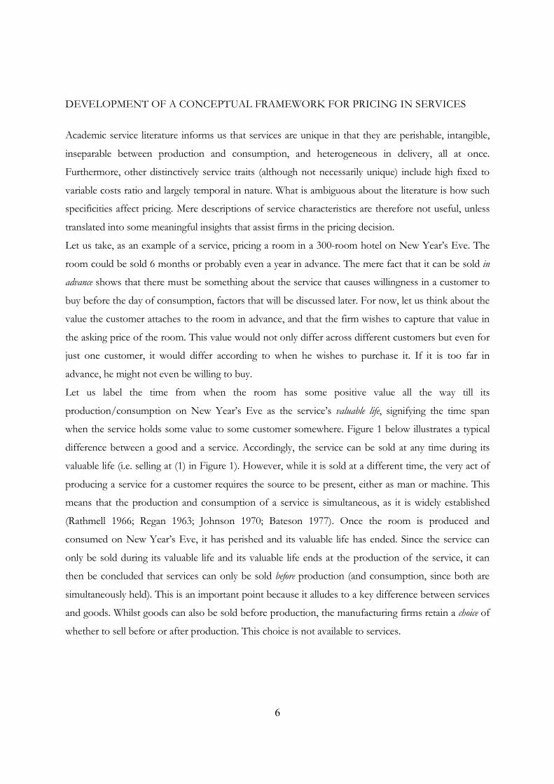
Let us label the time from when the room has some positive value all the way till its

production/consumption on New Year’s Eve as the service’s valuable life, signifying the time span

when the service holds some value to some customer somewhere. Figure 1 below illustrates a typical

difference between a good and a service. Accordingly, the service can be sold at any time during its

valuable life (i.e. selling at (1) in Figure 1). However, while it is sold at a different time, the very act of

producing a service for a customer requires the source to be present, either as man or machine. This

means that the production and consumption of a service is simultaneous, as it is widely established

(Rathmell 1966; Regan 1963; Johnson 1970; Bateson 1977). Once the room is produced and

consumed on New Year’s Eve, it has perished and its valuable life has ended. Since the service can

only be sold during its valuable life and its valuable life ends at the production of the service, it can

then be concluded that services can only be sold before production (and consumption, since both are

simultaneously held). This is an important point because it alludes to a key difference between services

and goods. Whilst goods can also be sold before production, the manufacturing firms retain a choice of

whether to sell before or after production. This choice is not available to services.

7

Figure 1: Buyer-Seller Exchange for a Typical Good and a Service

Sell

Buy

Production

Consumption

Seller

Consumers

Line of Perishability Inventory

Inventory

Delivery

Take Delivery

(1)

0t

Buyer-Seller Exchange for a Typical Good

Production and Delivery

Sell

Buy

Take Delivery and Consumption

Seller

Consumers

Line of Perishability

Sell

Buy

(2) (3)

0t At

Valuation Risk

Unavailability Risk

Service Valuable Life

APPq 000 δβα +−= 0PPq AAA δβα +−=

Buyer-Seller Exchange for a Service

8

Some may argue that certain services are actually produced in advance e.g. the production of a movie.

Undeniably, many services require its materials and equipment to be produced in advance such as a

hotel building, aircraft or even telecommunication towers. Yet, the value of a service is only unlocked

at the point when it is performed and consumed by the customer; the same value held by the customer

that can be converted into revenue to the firm through the price the customer is willing to pay. In the

case of the movie, the customer values the performance of the service by the firm (through the

provision of the movie, comfortable seating, quiet surroundings etc.), which is simultaneously

consumed by him or her. Without the customer’s consumption, which can only arise if the firm

produces the service, the value of the service cannot be converted into revenue, despite the production

of its equipment.

It ought to be clearer now that the issue of pricing in service is therefore the issue of advanced pricing,

even though the time in advance may be mere minutes e.g. the purchase of a movie ticket just before

the movie (cf. Edgett and Parkinson 1993) (i.e. at (3) in Figure 1).

Stylized Fact 1: The perishability and inseparability of services results in all sale of services to be advanced sales and

pricing of services to be advanced pricing

As Figure 1 shows, the inventory of a good is with the seller after production and before delivery and

with the buyer after taking delivery until consumption. Since services are intangible, there is no

question of inventory in the exchange. Rather, if the service customer buys in advance, he faces several

risks, which this study will elaborate below.

Since production and consumption is simultaneous, the consumer is unable to buy in advance to store

and consume at some later date. The consumer can only buy in advance and consume later. Similarly,

the firm can only sell in advance and produce later. This is an important point. Conventional economic

wisdom informs us that we buy only when the utility we attach to consuming the product outweighs

the price we are supposed to pay for it. However, normative economics and marketing literature often

implicitly assume that buyers receive utility at the time of purchase. Since there is now a separation of

time between purchase and consumption, it implies that the consumer’s utility is truly obtained not at

the time of purchase, but at the point of consumption (cf. Shugan & Xie 2000). Why is this significant?

When there is a separation of purchase and consumption, there is a probability that a buyer who has

purchased may not be able to consume, or as academics would term it – the utility becomes state

dependent (cf. Karni 1983; Fishburn 1974; Cook & Graham 1977). Put simply, a buyer who buys a

9

movie ticket an hour before the movie might find that he is unable to watch the movie when the time

comes because he has fallen ill. How is this different from goods? After all, when a consumer buys a

good, the consumption of his good is also dependent on his state at that time. The difference between

a good and a service in this regard is that for goods, the consumer chooses the time (and the state) that

is most suitable for consumption, after he has purchased the good e.g. taking a can of coke out of a

fridge to drink on a hot day. This is possible because the good is not immediately perishable upon

production. The service consumer may not have such a luxury since he needs to buy the service first

and then consume later, when the state is uncertain. The application of state dependent utility theory

into service research was first proposed by Shugan and Xie (2000), when they investigated spot and

advance pricing decisions and the optimality of advanced selling.

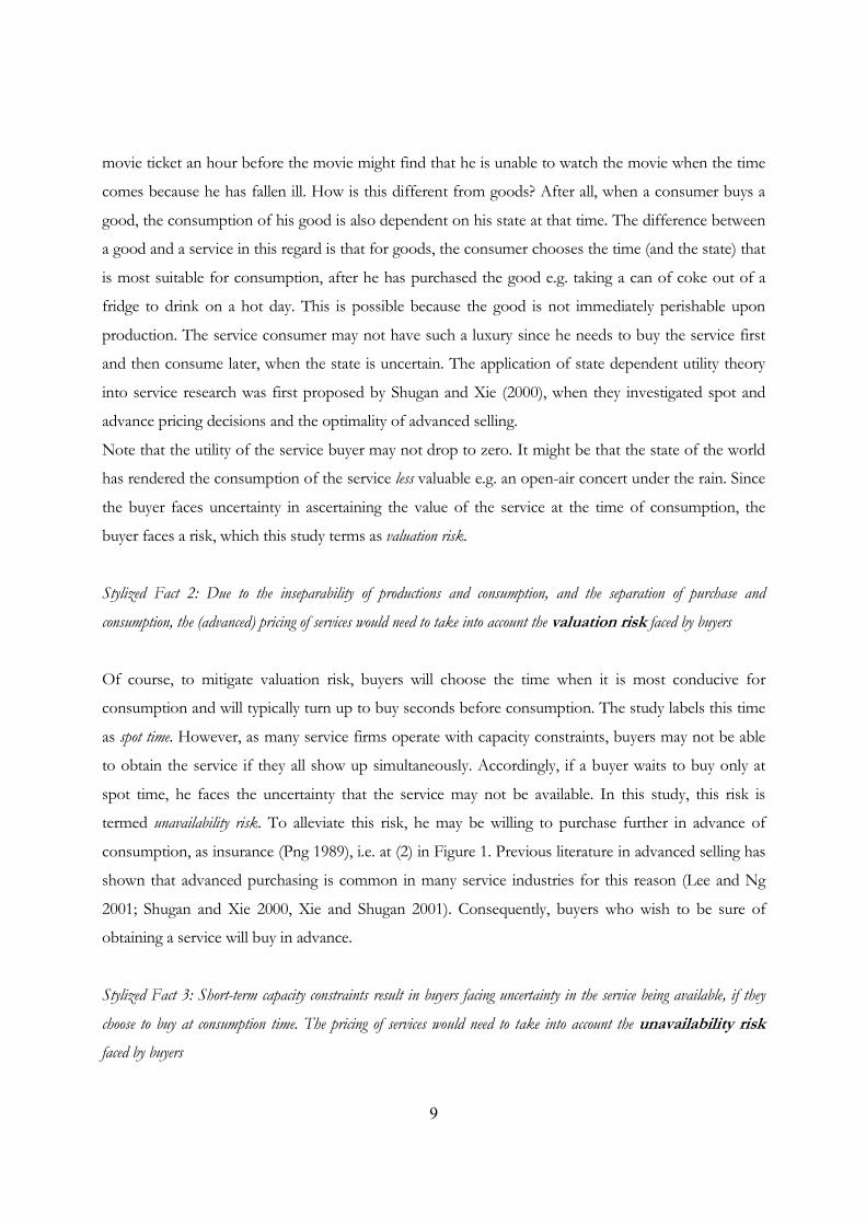
Note that the utility of the service buyer may not drop to zero. It might be that the state of the world

has rendered the consumption of the service less valuable e.g. an open-air concert under the rain. Since

the buyer faces uncertainty in ascertaining the value of the service at the time of consumption, the

buyer faces a risk, which this study terms as valuation risk.

Stylized Fact 2: Due to the inseparability of productions and consumption, and the separation of purchase and

consumption, the (advanced) pricing of services would need to take into account the valuation risk faced by buyers

Of course, to mitigate valuation risk, buyers will choose the time when it is most conducive for

consumption and will typically turn up to buy seconds before consumption. The study labels this time

as spot time. However, as many service firms operate with capacity constraints, buyers may not be able

to obtain the service if they all show up simultaneously. Accordingly, if a buyer waits to buy only at

spot time, he faces the uncertainty that the service may not be available. In this study, this risk is

termed unavailability risk. To alleviate this risk, he may be willing to purchase further in advance of

consumption, as insurance (Png 1989), i.e. at (2) in Figure 1. Previous literature in advanced selling has

shown that advanced purchasing is common in many service industries for this reason (Lee and Ng

2001; Shugan and Xie 2000, Xie and Shugan 2001). Consequently, buyers who wish to be sure of

obtaining a service will buy in advance.

Stylized Fact 3: Short-term capacity constraints result in buyers facing uncertainty in the service being available, if they

choose to buy at consumption time. The pricing of services would need to take into account the unavailability risk

faced by buyers

10

Technically, both the purchase further in advance and the purchase at spot are deemed as advanced

purchases as stylized fact 1 has explained. However, for purpose of clarity, the study terms purchases

close to consumption as spot purchases and purchases further in advance as advanced purchases,

consistent with the terminology used by extant literature on this phenomenon. In reality, as elaborated

by Lee and Ng (2001), the point where advanced purchase ends and spot purchase begins is industry

specific and is also dependent on ‘rate fences’ erected by the seller. Rate fences are constraints or

conditions imposed by service firms to ensure minimal cannibalization of purchase. Consequently, the

service industry is host to a wide range of advanced prices called “forward prices, pre-paid vouchers,

super saver prices, advance ticket prices, early discounted fares, early bird specials, early booking fares,

and advance purchase commitments” (Xie and Shugan 2001).

Clearly, there is a trade off between the buyer’s unavailability risk and valuation risk. Hence, there

exists a market for selling the service far in advance for buyers who like to ensure that the service is

available, regardless of whether the seller is willing to sell to this market. Similarly, there also exists a

market for selling at (close to) consumption time for buyers who like to ensure that they are able to

consume.

As illustrated in Figure 1, the trade-off between unavailability risk (which drives consumers’ willingness

to buy further in advance) and valuation risk (which drives consumers’ willingness to buy closer to

consumption) means that the distribution of demand across the valuable life of the service becomes

important in the firm’s pricing decision. In this respect, the firm faces uncertainty in demand

distribution across time – if they sell too much too early at too low a price, they may lose the

opportunity to earn higher revenue from transient or last- minute customers but if they sell too little in

advance, they may be saddled with unused capacity. To many revenue management consultants,

accurate demand forecasting, coupled with dynamic optimization algorithms across time is key to

better pricing decisions and higher profitability for service firms.

However, the pricing problem does not end there. The firm’s decision on price also has an effect on

the buyers. For simplicity, it is assumed that there exists only two times in the service’s valuable life to

sell – advanced time, denoting selling the service far in advance and spot time, denoting the selling of

the service at a time closer to consumption. If the advanced price is low, the discount from spot price

might outweigh the valuation risk faced by spot buyers. Similarly, if the spot price is low, advanced

buyers might wait till spot to buy. Consequently, there is some degree of cross-time dependence

11

between advanced and spot demand. Once this principle is extrapolated across multiple selling times in

a service’s valuable life, the full extent of the firm’s complex pricing decision can be appreciated.

Finally, a crucial difference between pricing for services and goods is embedded in another effect of

inseparability. Even if a buyer is to buy in advance, advanced selling requires the buyer to still present

himself (or at least, the item that requires the service) at spot time. In other words, since services are

inseparable in consumption and production, each advanced buyer has to ‘show-up’ to consume.

Especially when the purchase is conditional upon a particular time of consumption, there will be a

fraction of advanced buyers that may not be able to consume the service during that specified time.

This is commonly acknowledged in various revenue management literature, where attempts have been

made to structure various reservation policies to minimize the impact of the cancellation and ‘no-

show’ concept of advanced selling. (e.g. Alstrup et al. 1986; and Belobaba 1989; Hersh and Ladany

1978; Lieberman and Yechiali 1978; Rothstein 1971 1974 1985; Thompson 1961; Toh 1985). What has

not been discussed is that the existence of a non-zero probability of non-consumption by advanced

buyers provides a service firm with a unique opportunity not presented to goods firm i.e. the ability to

sell the capacity that was already sold in advance – again at spot. This re-selling capability may then

translate into additional profit for the firm either in the additional spot sales or overselling beyond the

firm’s capacity in advance. If this sounds distinctively implausible, let this study illustrate this point

through two examples. First, tow truck services operate with limited capacity but sell (albeit at a very

low price) through the Automobile Association (AA) an enormously large number of its services in

advance. Since the fraction of the market that actually requires a tow truck service may be low, the firm

obviously oversells its capacity in advance as well as re-sells them at spot (at a high price for those who

did not buy in advance). Second, IT support services are usually oversold to buyers in advance since

the fraction of non-consumption may be high.

The implications on the pricing decision are enormous. Depending on the demand distribution across

time, the level of non-consumption and capacity, firms might be prepared to manipulate advanced and

spot prices to optimize profits.

Stylized Fact 4: Separation of purchase and consumption due to the inseparability of services result in a non-zero

probability of advanced buyers not consuming, thus freeing up of capacity to be re-sold at spot. Pricing decisions have to

take into account the non-consumption effect.

12

In the following section,, the paper will examine this advanced sale phenomenon, given the above

propositions, through the development of a theoretical model. Few literature have investigated this

phenomenon. Desiraju and Shugan (1999) evaluated strategic pricing in advanced selling and found

that yield management pricing systems such as discounting, overbooking and limiting early sales work

best when price insensitive customers buy later than price sensitive customers. Shugan and Xie (2000)

showed that due to the state dependency of service utility, buyers are uncertain in advance and become

certain at spot while sellers remain uncertain of buyer states at spot because of information asymmetry.

They suggest that advance selling overcomes the informational disadvantage of sellers and is therefore

a strategy to increase profit. Xie and Shugan (2001) studied when advanced selling improves profits

and how advanced prices should be set. They have also investigated the optimality of advanced selling,

investigating selling in a variety of situations, buyer risk aversion, second period arrivals, limited

capacity, yield management and other advanced selling issues.

Png (1989) showed that costless reservations in advance is a profitable pricing strategy as it induces

truth revelation on the type of valuation that consumer has for the service (which is private

information). If the consumer has a high valuation i.e. ability to consume, he will exercise the

reservation and pay a higher price. If not, the consumer will not exercise. In another paper, Png (1991)

compared the strategies of charging a lower price for advanced sale and attaching a price premium at

the date of consumption versus charging advanced buyers a premium and promising a refund to

advanced buyers should consumption prices be lower than what was purchased.

However, despite various literature modeling the phenomenon, there has been no attempt to uncover

the theoretical foundations that drive the primitive consumer behavior of advanced selling i.e. the

notion of why advanced and spot demand exists, or how demand dynamics function within this

domain. Although the above literature model sellers’ pricing strategies on advanced selling, the

fundamental aspect of pricing lies in demand behavior. This demand behavior, particularly in the

advanced selling context, should not be exogenous and needs to be understood in at least two

dimensions. First, as modeled by Xie-Shugan, Shugan-Xie and Png, it is important to understand the

ways buyers react to changes in prices by their choice of buy, not-buy or switch to buy at a different

time. Second, it is also important to know how many will decide on each of the choices. In the latter,

the heterogeneity of buyers is a necessary factor and has yet to be studied. Lee and Ng (2001), however

did study the heterogeneity of buyers through the use of demand functions. However, the model

assumed that all advanced buyers were able to consume at the time of consumption, and that only

13

such buyers were captured within the demand functions. Furthermore, the model assumed that

demand at spot is independent of advanced price. This study does not make these assumptions.

Therefore in studying this phenomenon, three primary differences are highlighted between this study

and those above. First, this investigation does not model the individual consumer as one (or more) set

of homogeneous consumers. Instead, it models the consumers as heterogeneous, through the use of

demand functions. By modeling the consumers’ price sensitivity, both the decision of buyers to buy or

not to buy as well as the quantities of each choice at a given price are captured. Second, the

investigation also models the substitutability between advanced and spot demands, capturing the

buyers switching decisions, as well as the quantities that switch for a change in price. Finally, the model

explicitly captures the probability of advanced buyers who are not able to consume at the time of

consumption and how this impacts pricing is analyzed. Through this model, it is hoped that there will

be greater applicability in the characterization of the phenomenon.

Similar to this phenomenon is the concept of option pricing. Options are generally defined

as a binding contract between two parties in which one party has the non obligated right to buy or

sell some underlying asset. They are commonly a form of insurance against fluctuations in prices of

commodities or some common stock. However, option prices deals only with a price option, and if

the option is exercised, there is no uncertainty on being able to obtain the asset. In advanced selling,

an option to buy is often accompanied by a capacity guarantee although there is no guarantee of

high valuation at the time of consumption while in spot selling, the purchase has no guarantee that

the service is available i.e. no contract.

All proofs of propositions are found in the appendix.

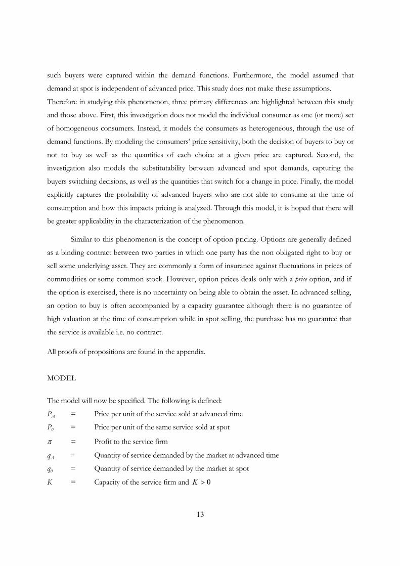
MODEL

The model will now be specified. The following is defined:

PA = Price per unit of the service sold at advanced time

P0 = Price per unit of the same service sold at spot

π = Profit to the service firm

qA = Quantity of service demanded by the market at advanced time

q0 = Quantity of service demanded by the market at spot

K = Capacity of the service firm and 0>K

14

At = Advanced time

0t = Spot time

A service sold in advance and at the time of consumption is not unlike two firms selling products

differentiated only by the time of sale. The difference is that since there is only one service firm, the

maximized profit is derived from demand at both times. Consequently, we can adapt product

differentiation models derived from economics literature. Following Dixit (1979) and Singh and Vives

(1984), we assume the following demand structure for selling the service at At and 0t :

APPq δβα +−= 00

0PPq AA δβα +−=

where 0>β , 0>δ and δβ >

Forms of this demand curve have been used in marketing modeling literature e.g. McGuire and Staelin

(1983), who modeled the decision of two manufacturers and their choice to intermediate when the

demand faced by both are represented by linear demand functions similar to that modeled above and

Ingene and Parry (1995) who modeled two competing retailers also facing similar demand functions,

and how a manufacturer would coordinate the channels.

Capacity and State effect

The parameter δ depicts the effect of increasing AP on 0q and increasing 0P on Aq . The

assumption δβ > means that the effect of increasing 0P ( AP ) on 0q ( Aq ) is larger than the effect of

the same increase in AP ( 0P ) i.e. own time-price effect dominates the cross time price effect. This is a

reasonable assumption because the price of a service is more sensitive to a change in the quantity at its

own time than to a change in the quantity across time, in other words, to borrow the terminology used

in models of this nature, own-time effect dominates cross-time effect. This could be, due to several

reasons, for example, the fact that the services are differentiated by time, the time difference may

create other uncertainties to the buyers and thereby result in a lower cross time effect.

Note that the parameter δ , in the context of advanced selling of services, can be deemed to capture

the valuation and unavailability risks faced by buyers. This means that a change in spot price would

have an impact on advanced demand and the degree of impact is dependent on the magnitude of δ . It

is assumed, for convenience, that the demand functions are symmetric across time. This assumption

will be relaxed later. Thus, if the unavailability and valuation risks are low, δ may increase, implying

that there is increased substitutability between buying in advance and at spot.

15

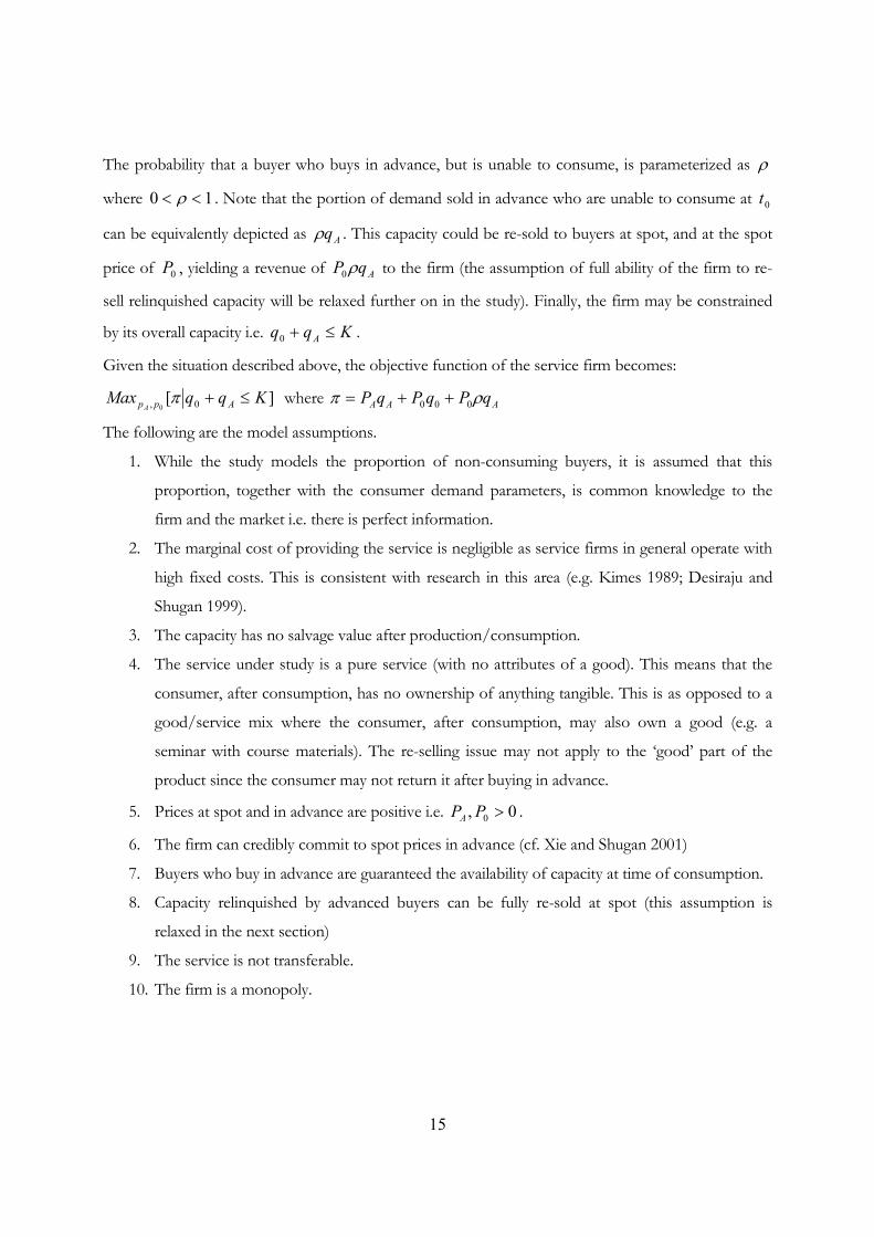
The probability that a buyer who buys in advance, but is unable to consume, is parameterized as ρ

where 10 << ρ . Note that the portion of demand sold in advance who are unable to consume at 0t

can be equivalently depicted as Aqρ . This capacity could be re-sold to buyers at spot, and at the spot

price of 0P , yielding a revenue of AqP ρ0 to the firm (the assumption of full ability of the firm to re-

sell relinquished capacity will be relaxed further on in the study). Finally, the firm may be constrained

by its overall capacity i.e. Kqq A ≤+0 .

Given the situation described above, the objective function of the service firm becomes:

][ 0, 0KqqMax AppA

≤+π where AAA qPqPqP ρπ 000 ++=

The following are the model assumptions.

1. While the study models the proportion of non-consuming buyers, it is assumed that this

proportion, together with the consumer demand parameters, is common knowledge to the

firm and the market i.e. there is perfect information.

2. The marginal cost of providing the service is negligible as service firms in general operate with

high fixed costs. This is consistent with research in this area (e.g. Kimes 1989; Desiraju and

Shugan 1999).

3. The capacity has no salvage value after production/consumption.

4. The service under study is a pure service (with no attributes of a good). This means that the

consumer, after consumption, has no ownership of anything tangible. This is as opposed to a

good/service mix where the consumer, after consumption, may also own a good (e.g. a

seminar with course materials). The re-selling issue may not apply to the ‘good’ part of the

product since the consumer may not return it after buying in advance.

5. Prices at spot and in advance are positive i.e. 0, 0 >PPA.

6. The firm can credibly commit to spot prices in advance (cf. Xie and Shugan 2001)

7. Buyers who buy in advance are guaranteed the availability of capacity at time of consumption.

8. Capacity relinquished by advanced buyers can be fully re-sold at spot (this assumption is

relaxed in the next section)

9. The service is not transferable.

10. The firm is a monopoly.

16

Furthermore, the model assumes a high congruence between what the seller sells and what the buyers

believe they are buying. For example, a movie, a flight, a hotel room, tow truck service, annual auditing

can all be considered (almost) homogeneous units of services because what the buyer expects to

consume is similar to what the seller expects to produce. Whilst it is acknowledged that services are

heterogeneous, the heterogeneity is usually at the point of consumption and it is assumed that the

degree of service heterogeneity expected by prospective buyers do not sufficiently influence the value

they place on the service in advance of consumption. Hence, the heterogeneity in demand lies only in

buyers’ valuation of the service and not because of perceived differences in the service offering.

A few noteworthy comments on the firm’s objective function are necessary at this juncture. First, it is

assumed the firm maximizes its profit in one stage, despite the profit being derived across two times

i.e. advanced and spot. This is because of the assumption of perfect information. Since all parameters

of demand at both times are common knowledge to the firm, the firm would be strategic in

maximizing and manipulating its prices for both times. Certainly if information is not perfect, the

model could be modeled in a variety of ways e.g. in two stages strategic pricing through backward

induction, or with myopic pricing where the firm maximizes profit in advance and then at spot (cf.

Jagpal 1998). The purpose here is to understand the phenomenon in its idealized form, without setting

specific conditions.

The Xie-Shugan model depicts the phenomenon as a two-period process where homogeneous

consumers arriving in period 1 can decide to buy or wait after the firm announces their spot and

advance prices. Consumers may also arrive in period 2. In reality, buyers are not merely heterogeneous

in their valuation of the service (i.e. own time price sensitivity). They are also heterogeneous in

their willingness to switch between spot and advanced time (cross time sensitivity).

In Png’s model, the advance buyer, should he chooses to buy, knows how much he values the

service only at the time of consumption. The probability of the buyer turning out to be a low or

high valuation customer is depicted as λ (in Xie-Shugan, it is q). This model incorporates this

feature with ρ . If the buyer is able to consume, he is deemed to be a high valuation buyer. If he is

unable to consume, he is deemed to have a low valuation. However, a key difference is that Png

assumes a low valuation customer obtains a low valuation regardless of his ability to consume i.e.

if he consumes, he receives a low valuation and if he does not, he will enjoy a low valuation net of

any price paid for the alternative. (Png 1989, p 250) Although it may not make a difference to the

customer who obtains a low valuation regardless, his willingness to consume the service has a

17

direct effect on the firm. If he does not consume, the capacity can be relinquished and re-sold. This

ability to re-sell obviously impacts on the price of the service, both in advance and at spot. In all of

Png, Xie-Shugan and Shugan-Xie’s models, this ability had not been considered and the study has

incorporated it here.

ANALYSES

When capacity is higher than optimal demand (interior solution), the constraint is non-binding and

the study provides the following lemma as a benchmark:

Lemma 1: When 0=ρ and the capacity constraint is non-binding, )(2

*

0

*

δβα−

== PPA which

we denote as )0(*P , and 2

*

0

* α== qqA which we denote as )0(*q and

)(2

2*

δβα

π−

=

which we denote as )0(*π .

If the fraction of non-consumption capacity is zero 0=ρ , i.e. all advance buyers are able to

consume, prices and quantities sold at 0t and At will be the same, due to the symmetric demand

functions. This is illustrated in Figure 2 below.

Figure 2: Characterization of the Non-consumption effect

*

AP

1

**

0 , APP *

0P

ρ

)(2 δβα−

0

**

0 , Aqq *

Aq

2

α

18

As the study has argued previously, ρ will always take on a positive value. Consequently, prices

and quantities at 0t and At start diverging, as the following proposition show:

Proposition 1: When 0>ρ , the firm derives a higher profit by lowering advanced price

and increasing spot price such that

[ ]( ))2()(21)0(** δβρδβ −+−⋅−= SPPA

[ ]( )ρβδβ +−⋅+= )(21)0(**

0 SPP

and obtains a higher advanced demand but lower spot demand such that

[ ]( )ρβδβ ++⋅+= )(21)0(** SqqA

[ ]( ))2()(21)0(**

0 δβρδβ +++⋅−= Sqq

where

)])(4 2222 ρβδββρ

−−=S and 0, *

0

* >PPA if and only if 24

2

ρδβ

−⋅> .

As every unit of advanced demand provides an opportunity to the firm to re-sell, the firm chooses

to lower *

AP to obtain a higher advanced demand. Due to cross time sensitivity, a lower *

AP

decreases spot demand. However, instead of compensating by lowering *

0P to obtain higher spot

demand, the firm chooses to increase *

0P instead since resold capacity can be sold at a premium

and the marginal revenue from re-selling capacity at a premium (through higher *

0P ) is higher than

marginal revenue derived from increasing spot demand through a lower *

0P . A graphical

representation of the above can be seen above in Figure 2. Notice that the solutions are conditional

19

on)4(

2

2ρδβ

−⋅> . This means that the ability of a firm to obtain positive revenue from selling

in advance is dependant on the degree of own-time price sensitivity vis-à-vis the cross time price

sensitivity. Notice that S exists only when 0>ρ . Thus, while the terms proceeding S determine

the level of increase or decrease in prices and quantities, we can intuitively label S as the non-

consumption effect attributable to the advanced purchase of services.

To highlight the impact on profit, the difference in expected profits (after some manipulation) can

be written as

Lemma 2:

)5()4()3()2()1()0(** −+++=−ππ where

)5(

)4(

)3(

)2(

)1(

[ ][ ][ ][ ][ ]ρδρβρβδβ

βρδββρδβρβρδβρβρδβρ

ρ

2222222**

2**

**

**

**

44)(4)0()0(2

)(2)(2)0()0(

)(2)0()0(

)(2)0()0(

)0()0(

−++−⋅

+−++⋅

++⋅

+−⋅

SqP

SqP

SqP

SqP

qP

The first term is the added profit due to double selling the fraction of non-consuming capacity,

)0(qρ . The second shows that the capacity that is double-sold is sold with a price premium of

[ ]βρδβ +−⋅ )(2S . The third term shows that the advanced demand also increases, amplified by

the combination of both own-time and cross-time sensitivities i.e. [ ]βρδβ ++⋅ )(2S . This

amplification is because advanced demand is made higher through both a higher spot price and a

lower advanced price. The fourth term shows that the increase in advanced demand also enjoys the

same price premium. Finally, the fifth term captures the loss in revenue as a result of a lower

advanced price and a lower spot demand.

Lemma 1 is consistent with Xie-Shugan’s model where it was shown that when marginal

cost is low and capacity constraint is non-binding, advance and spot prices are the same.

However, unlike Xie-Shugan, the findings show that advanced prices may be lower even when

marginal costs are zero as the presence of ρ creates the divergence in advance and spot prices.

Clearly, the potential revenue from one unit of advanced sale is higher than that from spot sale.

Therefore, advanced price decreases to generate a higher advanced demand. The cross time

effect of this is an even higher spot price.

20

As ρ increases, the firm has a greater incentive to price AP lower to stimulate advanced demand.

This amplifies the decrease in spot demand, pushing 0P even higher.

Proposition 2: The greater the probability of non-consumption, the higher (lower) the

quantity sold in advance (at spot) and the lower (higher) the advance (spot) price

i.e. 0*

<∂

∂

ρAP

, 0*

0 >∂

∂

ρP

and >∂

∂

ρ

*

Aq, 0

*

0 <∂∂ρq

.

In Png’s model, a strategy of selling firm advanced order does not maximize profit

because the advanced buyer is unwilling to pay a higher price due to unavailability and valuation

risk. Yet, a firm advanced order usually guarantees availability and as Xie-Shugan model

showed, firm advance orders can be optimal. In addition, Png’s model does not take into

account the fact that a buyer who buys in advance has a non-zero probability of not consuming

and that non-consumption frees up the capacity to be re-sold. By modeling in non-consumption,

the study shows that the potential revenue from advanced sales increases and it may be optimal

for the firm to sell in advance.

Png’s model also showed that the seller’s revenue from spot sales is zero because buyers

would prefer the non-contingent alternative in advance rather than wait till spot where the seller

would extract all the consumer’s surplus (i.e. high price). Where the market is heterogeneous in

the form of a demand function, the optimal price at spot assumes not all surpluses are extracted

from everyone. Consequently, there is also heterogeneity in the degree to which customers may

be willing to wait till spot or buy in advance. This implies that both spot and advanced demand

would exist, with some degree of substitutability between buying at these two times, as modeled

here. Accordingly, there is an optimal price at both times, as set out above in proposition 1.

MODEL EXTENSION: OFFERING A REFUND WHEN THE ABILITY TO RE-SELL AT

SPOT IS PROBABILISTIC

Providing refunds for buyer’s inability to consume is widely practiced in the airline industry.

Casual enquiries by the author with airlines sales offices indicated that many airline tickets are sold

with some refund value. Some tickets even provide a full refund to the customer. Generally, a full

21

refund means that the ticket purchased can be returned to the airline for a complete reimbursement

of the price at any time – even after the proposed date of travel. This means that if the buyer cannot

make a flight for any reason, the airline is fully prepared to return the price of the air ticket to the

customer without any penalty fee, no questions asked. Furthermore, many airlines allow a refund

on non-utilized sectors, e.g. if the consumer has purchased a return ticket but only utilized one leg

of the ticket.

There is a fundamental difference between a full refund of this nature and those given out by

retail shops for goods purchased by service firms after the consumption of the service. In the

latter, the refund is given (or promised) if the firm fails the consumer i.e. the compensation is

provided to the buyer due to firm’s failure to deliver the benefits, according to the buyer’s

perception. In the former, and also the focal point of this study, refunds are promised for buyer

failure i.e. when the buyer fails to consume the service, through no fault of the firm. The use of

the term ‘buyer failure’ is chosen for ease of explanation and is entirely from the perspective of

the firm. From the firm’s perspective, their guarantee of capacity when selling in advance is

usually in return for the buyer’s guarantee to consume. If the buyer doesn’t, he is deemed to

have ‘failed’. Certainly from the buyers’ perspective, they could argue that they have a right to

demand for a refund since they have not yet consumed the service. What this study aims to

investigate, by extending the current model, is whether there is any benefit to the firm, revenue-

wise, if the firm had to provide that refund.

Png’s (1989) model attempted to shed some light on this phenomenon. While he found that firms’

advance orders are not optimal, his study showed the profit maximizing strategy is to insure the

risk averse customer by compensating him when his valuation low and charging him high when his

valuation is high. Thus the optimal result was a costless reservation at advanced time for all

advanced buyers and a higher price for the high valuation customer at spot with the low valuation

buyer not exercising the reservation. In this way, the advanced buyer is fully insured against

capacity unavailability and partially insured against his valuation at spot time. However, this

strategy requires the advanced buyer to face the risk of unavailable capacity at the time of

consumption. In other words, Png’s advanced buyer does not actually buy the service; he merely

buys the option of purchasing the service at the time of consumption, at a stipulated price i.e. a

price option. This is in contrast to the buyer failure refund of the type illustrated above where it is

22

clear that the buyer buys with a firm advance order (where capacity is guaranteed) with a refund in

the event of a low valuation.

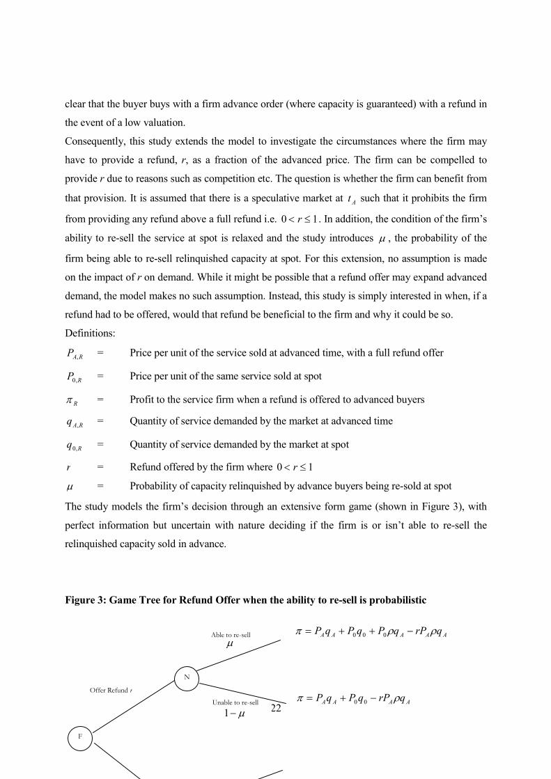
Consequently, this study extends the model to investigate the circumstances where the firm may

have to provide a refund, r, as a fraction of the advanced price. The firm can be compelled to

provide r due to reasons such as competition etc. The question is whether the firm can benefit from

that provision. It is assumed that there is a speculative market at At such that it prohibits the firm

from providing any refund above a full refund i.e. 10 ≤< r . In addition, the condition of the firm’s

ability to re-sell the service at spot is relaxed and the study introduces µ , the probability of the

firm being able to re-sell relinquished capacity at spot. For this extension, no assumption is made

on the impact of r on demand. While it might be possible that a refund offer may expand advanced

demand, the model makes no such assumption. Instead, this study is simply interested in when, if a

refund had to be offered, would that refund be beneficial to the firm and why it could be so.

Definitions:

RAP , = Price per unit of the service sold at advanced time, with a full refund offer

RP ,0 = Price per unit of the same service sold at spot

Rπ = Profit to the service firm when a refund is offered to advanced buyers

RAq , = Quantity of service demanded by the market at advanced time

Rq ,0 = Quantity of service demanded by the market at spot

r = Refund offered by the firm where 10 ≤< r

µ = Probability of capacity relinquished by advance buyers being re-sold at spot

The study models the firm’s decision through an extensive form game (shown in Figure 3), with

perfect information but uncertain with nature deciding if the firm is or isn’t able to re-sell the

relinquished capacity sold in advance.

Figure 3: Game Tree for Refund Offer when the ability to re-sell is probabilistic

Offer Refund r

Unable to re-sell

µ−1

AAAAA qrPqPqPqP ρρπ −++= 000 Able to re-sell

µ

F

N

AAAA qrPqPqP ρπ −+= 00

23

ANALYSES

First, consider the impact of µ , if the firm does not have to offer a refund i.e. 0=r . From

proposition 2, an increase in probability of non-consumption ρ decreases advanced prices and

increases overall spot prices. However, for a given ρ , if µ is low, the impact of ρ is lessened

even if ρ is high. The proposition below follows:

Proposition 3: A decrease in the firm’s ability to resell increases advanced prices and

reduce spot prices.

Clearly, the presence ofµ reverses the effect of ρ . The above proposition is consistent with

propositions 1 and 2. When the firm has a low probability of re-selling at spot market, advanced

prices increase because the inability to sell reduces the firm’s incentive to price lower and stimulate

the advanced market. Thus, prices in advance increase and spot prices decrease to the extent that if

0→µ , )0(, **

,0

*

, PPP RRA → .

When is a refund offer more profitable? This should be when:

]}[{]}[{ norefundrefund EMaxEMax ππ >

The proposition below illustrates the benefit of offering a refund:

Proposition 4: A positive refund could be more profitable to the firm if and only if the

cross-time price sensitivity is low i.e. when φβδ ⋅< where

24

2

2222

24

))1()42(4()2)(1(2

µρρµρµρµµρρρµµρ

φ+−

−−−−−−++=

and 10 << φ for all permitted values of 10 << ρ and 10 << µ

and firm prices at ( ))]2)()(2[1)0(**

, µδρδβµρδβ −++−−= rSPP RRA ,

( )]2)()(2[1)0(**

,0 ρβδβµρδβ rrSPP RR −++−+= and obtains

( ))]()(2[1)0(**

, rSqq RRA δβµρδβ −+++= ,

( ))]22()()(2[1)0(**

,0 δµβρδβµρδβ −−−++−= rrSqq RR

where ]2)2()44([

)(222222 βδµρρδρµρβ

δβµρrrr

rSR +−−−−

−=

Note that SSR → when }1,0{ →→ µr .

Xie-Shugan showed that firm advanced orders with a refund offer may be optimal as the firm is

able to obtain a higher price in advance to compensate for the cost of refund, as well as derive

greater profits from cost savings in not having to serve these customers. The above proposition

shows that the firm could derive higher revenue from either (or both) higher prices and higher

advanced demand when a refund is offered.

If the cross-time sensitivity is low i.e. φβδ ⋅< , the refund offer actually increases profit to the

firm. This is because when the cross time impact of a price change is low (i.e. less customer

switching), a change in price at (advanced) spot time would have less an impact on (spot) advanced

demand. Low cross time sensitivity implies state sensitive people are more concerned about a

conducive state and won’t switch to advanced time even if the price is low. Similarly, capacity

sensitive people are more concerned about obtaining the service, and will not switch to spot time

even if the spot price is low. Consequently, a refund offer effectively reduces the price paid for the

advanced buyer who may not consume without any impact on the buyer who will consume. When

cross time sensitivity is low, this reduction in price does not cause as many spot buyers to switch,

hence the firm obtains higher profit from higher revenue in advance without losing much spot

revenue.

25

Proposition 5: When βµρρ

ρµρµρδ ⋅

−−−−+

≤)1(2

)1(2)1(, the firm should offer the boundary

solution of a full refund (i.e. 1* =r ).

Since the firm is constrained by speculators, it cannot increase refund beyond giving a full refund.

Thus, the above proposition spells out the level of cross time sensitivity when the refund offered is

a boundary solution of a full refund. As noted in proposition 3, the ability to re-sell capacity

relinquished by advanced buyer contributes to the level of advanced price. Consequently, under the

condition of full ability to re-sell, the study finds the following counter intuitive proposition:

Proposition 6: When 1=µ , ρδ

β > and the refund offered increases profit (under the

condition in proposition 4) and

)]2(2[

4)34()1(4)2(222

2232233

ρρβδρδρβδρρδβρδρρβ

−−+−++−+++

<r , **

, ARA PP < .

In contrast to Png and Xie-Shugan models, the above proposition shows that advanced price may

be lower with a refund offer. This is because the firm derives higher revenue from two sources.

First, the revenue from increase demand may outweigh the revenue from increased price. Second,

with an expanded advanced demand, the potential revenue from non-consumption also increases.

Consequently, when price sensitivity is high relative to cross-time sensitivity i.e. ρδ

β > , the result

can be pareto optimal where it is possible for the firm to provide the advanced buyer with

insurance against capacity unavailability (through a positive advanced purchase price) and

insurance against valuation risk (through a refund offer), at a price that may be lower than if a

refund is not offered.

Asymmetric Cross time Sensitivity

As noted earlier, the parameter δ , in the context of advanced selling of services can be deemed to

capture the trade off between valuation and unavailability risks. Clearly, they do not need to be the

same i.e.

26

APPq 000 δβα +−=

0PPq AAA δβα +−=

where 0>β and 0,δδβ A>

To investigate the implications of asymmetry, this study takes two extreme examples i.e. 0→Aδ

and 00 →δ . For simplicity, it is assumed no refund is provided and capacity relinquished by

advanced buyers would be fully sellable i.e. 1=µ , r = 0.

When 0→Aδ

In this case, advanced demand is not affected by spot prices. However, spot demand may be

affected by prices in advance and at spot. This type of behavior can be typical of a market segment

where capacity availability is extremely important. Such services may include those where the time

of consumption is tied to the value of the service e.g. an important flight, a hotel room on New

Year’s eve, an anniversary dinner etc. In these cases, the advanced market cannot be persuaded to

wait to buy at spot. If the price in advance is too high, they will seek alternatives at advanced time

(and therefore drop out of the market) instead of switching to spot. This is termed as a market that

faces high unavailability risk.

When 00 →δ

In this case, spot demand is not affected by advance prices. However, advanced demand may be

affected by prices in advance and at spot. This type of behavior can be typical of a market segment

where a conducive state for consumption (i.e. high valuation) is extremely important. Such services

may include emergency services e.g. tow truck, or computer/equipment support services where the

precise time when the service is required is often not known. In these cases, the spot market cannot

be persuaded to buy in advance (high valuation risk). If the price at spot is too high, they will seek

alternatives at spot time (and therefore drop out of the market for the service). This is termed as a

market that faces high valuation risk.

In practice, a service can face a market with both high valuation and unavailability risk. For

example, a flight from London to New York will be a service with high availability risk for a

passenger that needs to get on a particular flight e.g. to attend his son’s graduation. He will

therefore purchase in advance. If the price is too high, he will choose an alternative (perhaps

27

another airline) but he will not consider waiting till spot, as he needs to be in New York at that

particular date. In contrast, a business executive who does not know when he may be called to go

on a business trip to New York will not be swayed to buy in advance, as he is unsure if he should

be traveling on that date.

Proposition 7: A market that faces high unavailability (valuation) risk pays higher prices

in advance (at spot) than a market that faces high valuation (unavailability) risk if

ρδ

β > .

Whilst the above proposition is not surprising, it is found that the firm’s profit from asymmetric

states is not the same. Since high unavailability risk can increase advanced price, it also serves to

reduce advanced demand as a result of the increase in price. This reduces the potential revenue

from non-consumption.

Proposition 8: If the magnitude of 0δ and

Aδ are the same, profits are higher when

00 →δ than when 0→Aδ .

When 00 →δ , the market faces high valuation risk. Since spot demand is not easily persuaded to

buy in advance, the firm will set spot prices higher. This, in turn, provides higher potential revenue

from advanced demand (through non-consumption). However, when 0→Aδ , unavailability risk

is high and this pushes up advanced prices, reducing advanced demand and thereby reducing

potential revenue from non-consumption. Consequently, profits are lower than when 00 →δ .

DISCUSSION

This study aims to offer a more applicable model of advanced selling as a phenomenon. Stylized

fact 1 justified why all services are sold in advance and that the pricing of services is in fact

advanced pricing. In stylized facts 2 and 3, the study proceeded to explain how advanced demand

may be distributed between a time further in advance until consumption due to the specificities of

services, particularly through the heterogeneous levels of unavailability and valuation risks faced

by the service consumer. In stylized fact 4, it illustrated one particular idiosyncratic factor of

advanced selling in services is illustrated i.e. the fact that advanced buyers may not be able to

28

consume and thereby releasing the capacity to be re-sold by the firm at the time of consumption.

Having conceptualized the factors that influence pricing in services, the study then proceeded to

model the phenomenon through a theoretical model incorporating consumer price sensitivity,

degree of cross time substitutability as well as the ability of the service firm to re-sell relinquished

capacity at spot time to derive the optimal pricing and quantities.

The model presented found, in proposition 1 that advanced prices are lower than spot prices even

without binding capacity constraints or marginal costs because the potential revenue from one unit

of advanced sale is higher than that from spot sale. Proposition 2 showed that as the probability of

non-consumption increased, advanced price decreased and spot prices increased further. This result

may be applied to emergency or support services where buyers can buy in advance with very low

probability of consumption. As noted earlier, an example of this would be breakdown services

where buyers buy in advance but their consumption date is uncertain. What may be seen as

insurance will in fact be a form of advanced purchase at a very low price, Without advanced

purchase, the spot price of breakdown services will be high, as many who own older vehicles will

attest. Another example of advanced purchase at a low price with a low probability of consumption

is the purchase of support services e.g. equipment or IT support. Such services are often sold to

individuals or firms on an annual subscription basis. Again, without a support contract, the spot

prices of such services are usually much higher.

The higher potential revenue from advanced demand diminishes, however, as the ability of the

firm to sell relinquished capacity reduces, as shown in proposition 3. Services that required

capacity scheduling or planning at the time of consumption such as removal or exhibition services

may fall into this category, where spot and advanced prices may be the same. Yet, this proposition

may accentuate the realization that such firms can explore creative pricing strategies or use

technological advancements to improve overall profit through the ability to manipulate the

parameters set out in this model.

For buyers that buy in advance but are unable to consume (i.e. buyer failure), it was found in

proposition 4 that offering a refund is optimal when cross time sensitivity is low relative to own-

time price sensitivity. This is because when cross time sensitivity is low, the firm benefits either

from increase price and/or increased advanced demand. Proposition 5 showed that a full refund

may also be optimal under conditions of very high own-time price sensitivity relative to cross time

sensitivity. However, proposition 5 is a boundary solution. Consequently, if the firm is able to

29

increase cross time sensitivity, profit may be increased with an interior solution for r. A counter

intuitive result was discovered in proposition 6, where a refund offer to advanced buyers may be

optimal with a lower advanced price than if refund was not offered. This occurred when the refund

offer is able to expand demand to such a degree that for the firm could lower its advanced price.

Asymmetric conditions where unavailability and valuation risks are not equal were then

investigated. Not surprisingly, the investigation found in proposition 7 that advanced prices were

higher when unavailability risks were high and spot prices were higher when valuation risks were

high. What was surprising at first was proposition 8 where the study showed that the two

asymmetric conditions did not yield the same profit i.e. profit was higher when the market faced

high valuation risk than when the market faced high unavailability risk. This was justified on the

realization that high valuation risks resulted in higher spot prices which in turn increased potential

revenue from the non-consumption of advanced buyers. Proposition 7 and 8 showed that the

perception of high valuation and high unavailability risks may be profitable for the firm. However,

if the risks are too high, buyers may not buy. In practice, such risks may be manipulated by the

firm through its pricing policies, for example, by providing some degree of flexibility in the time of

consumption. Where the business executive facing high valuation risk in not being certain about

which date he is to fly, a flexible flight time (e.g. open tickets) might persuade him to buy in

advance or lower his valuation risk, thus increasing his willingness to pay. Similarly, if the

graduate’s father is given a ticket that allows him to choose a range of flight times thereby reducing

his unavailability risk, he might be swayed to buy at the last minute or lower his perception of risk,

which will in turn increase his willingness to pay. A summary of the results of the model can be

seen in Table 1 below.

30

Table 1: Summary of Results

Impact of

increasing

non-

consumption

, ρ

Impact of

decreasing

ability to

re-sell, µ

Impact of

increasing

refund, r

Asymmetry

High unavailability risk

= 0→Aδ and High

valuation risk = 00 →δ

When

24

2

ρδβ

−⋅> When

ρδ

β >

and 1=µ

When ρδ

β >

Advanced

Price

Decrease Increase Decrease Higher when 0→Aδ than

when 00 →δ

Spot

Price

Increase Decrease Increase Lower when 0→Aδ than

when 00 →δ

Advanced

Demand

Increase Decrease Increase Lower when 0→Aδ than

when 00 →δ

Spot

Demand

Decrease Increase Decrease Higher when 0→Aδ than

when 00 →δ

Profit Increase Decrease Increase when

φβδ ⋅< (see

proposition 4)

Higher when 00 →δ than

when 0→Aδ

This model also resolved the issue of risk aversion in buyers through the use of a demand function.

Since buyers in advance are heterogeneous in their valuation of the service, their probabilities of

non-consumption are also heterogeneous. As advanced buyers also discount this uncertainty in

31

their valuation, this ‘discount’ alludes to the buyers’ degree of risk aversion. The demand function,

and its parameters, subsumes such complexities. The result was a parsimonious model that offered

a theoretical framework on how service pricing could be approached.

Revenue Management

The objective of revenue management studies is to maximize yield by managing the sale of service

capacity over time, through pricing, capacity allocation, and timing of sale (Badinelli and Olsen

1990; Desiraju and Shugan 1999). One of the limitations of current revenue management (RM)

literature is that many RM models maximize payoffs/yield, given some forecasted demand profile

that is largely exogenous, and does not explicitly capture the price/capacity relationship (e.g.

Badinelli and Olsen 1990; Belobaba 1989; Bodily and Weatherford 1995; Hersh and Ladany 1978;

Pfeifer 1989; Toh 1979). A widely used approach in this stream of literature is that of

mathematical programming. Kimes (1989), however, commented “although the linear

programming solution can be found, the assumption of deterministic demand makes the solution to

the problem unrealistic”. The model developed here is based on demand functions across time,

hence capturing fundamental concepts of consumer behavior (cf. Chase 1999; Lieberman 1993;

Relihan III 1989).

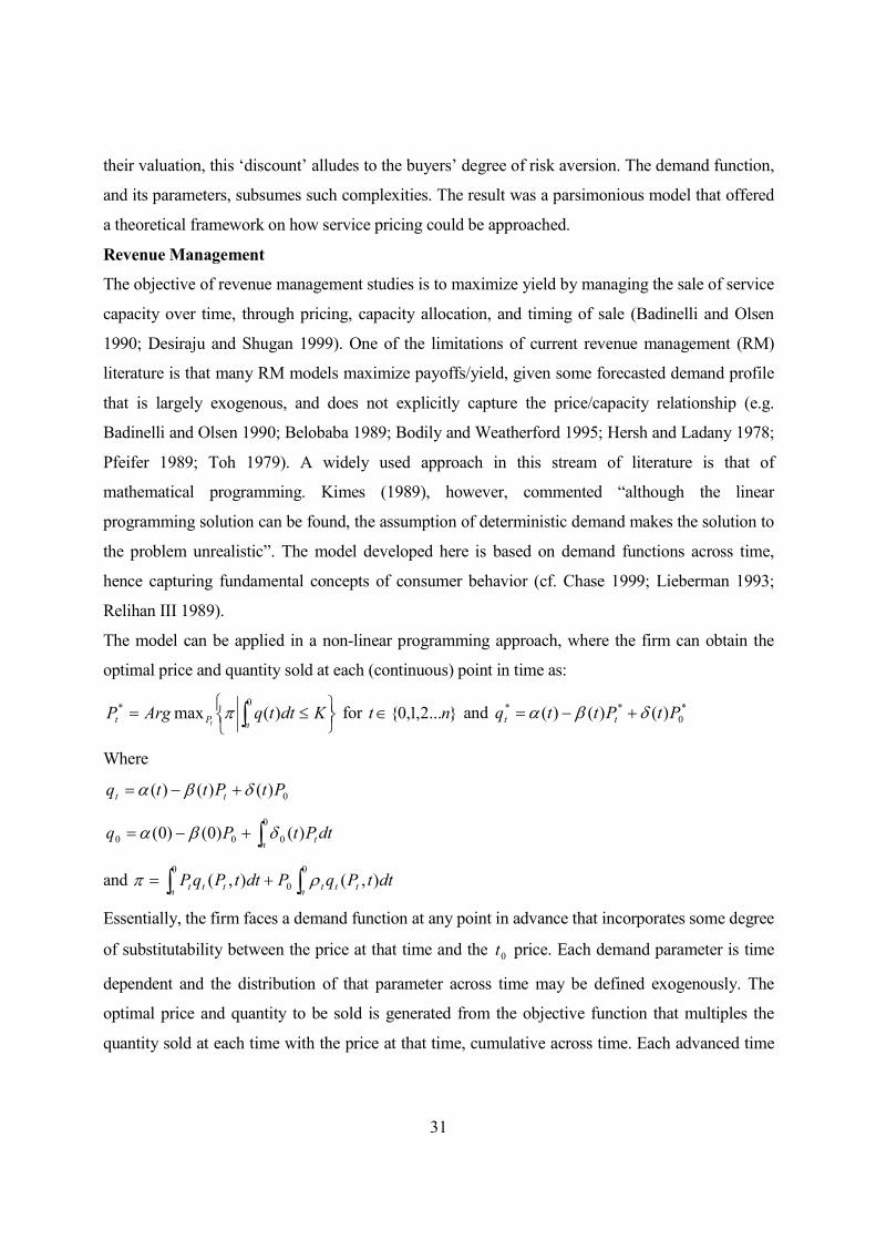
The model can be applied in a non-linear programming approach, where the firm can obtain the

optimal price and quantity sold at each (continuous) point in time as:

≤= ∫

0* )(max

nPt KdttqArgP

tπ for }...2,1,0{ nt ∈ and *

0

** )()()( PtPttq tt δβα +−=

Where

0)()()( PtPttq tt δβα +−=

∫+−=0

000 )()0()0(n

t dtPtPq δβα

and ∫∫ +=0

0

0

),(),(n

tttn

ttt dttPqPdttPqP ρπ

Essentially, the firm faces a demand function at any point in advance that incorporates some degree

of substitutability between the price at that time and the 0t price. Each demand parameter is time

dependent and the distribution of that parameter across time may be defined exogenously. The

optimal price and quantity to be sold is generated from the objective function that multiples the

quantity sold at each time with the price at that time, cumulative across time. Each advanced time

32

will also yield a fraction that may not be consumed at 0t and that is accounted for in the objective

function. Hence, the price and quantity relationship is captured explicitly as is the substitutability

between times of purchase. Price discrimination, by a simple extension, can simply be incorporated

into the model as the standard “affine” pricing schedule where the firm realizes a price premium at

any point in time equivalent to the social surplus at the optimum at any time t. Similarly, multi-leg

flights, 3 nights hotel stays etc. can be modeled in as a bundled product and its demand function

ascertained accordingly. By using the demand function, a vast quantity of economic literature can

be applied into the advanced selling context to produce richer insights into the strategy of advanced

selling.

In the past, where pricing is often static, the above specification might have been difficult to

implement. However, the advent of the connected economy, where data can be obtained quickly,

technological innovations have made complicated algorithms possible to implement. Thus, a

dynamic pricing model such as the one suggested above is not impossible. Furthermore, business

to business (B2B) and business to consumer (B2C) marketplaces create new ways to exchange

goods and services, and the firm has to innovate for higher revenues. What is left, is the question of

how many prices should the firm introduce to the market before it becomes confused (see Desiraju

and Shugan 1999). The purpose of this paper is not merely an additional model of revenue

management or to capture optimal pricing strategies. What it seeks to show, by abstracting the

phenomenon into this theoretical framework, is that the parameters modeled here provides the firm

with various strategic levers to influence demand and plan an effective pricing strategy. As noted

earlier, degree of flexibility may affect the perception of risk. Depending on the type of service

industry, further research and managerial creativity may find other levers that will manipulate the

demand faced by the firm and provide the firm with unique opportunities for higher revenue.

It is fairly common knowledge that many low cost airlines price according to the amount of

capacity available, increasing prices as the plane fills up, and according to demand forecast.

Consequently, revenue management is capacity and forecast centered rather than value centered.

Previous studies (e.g. Ng, Wirtz and Lee, 1999) have shown that such practices often result in

conflict between revenue managers and the sales and marketing department. This is not surprising,

as this paper has shown. When revenue management takes demand as exogenous and sales and

marketing strives to improve value to increase price/demand, conflicts will naturally occur. The

study shows that reconciliation between the two can be obtained by way of a more satisfying

33

approach towards revenue management, as a practice. The contention here is that the firm’s focus

should not merely be on revenue management as it should be on revenue improvement. Thus, only

when demand behavior is incorporated into the equation, providing a more complete picture, the

firm would be able to understand where and how its revenue is being obtained. As the model has

demonstrated, the offer of refund can increase profit for the firm. However, firms may

misunderstand that refund is merely a form of providing ‘quality’ service and as such, might be

tempted to drop the offer (as some low cost airlines do). In doing so, they miss the opportunity to

derive higher profits either through expanded advanced demand or higher advanced price.

CONCLUSION

For several decades, developed economies have been service economies. The expansion of the

service sector is partially attributed to an increase in the intangible component (often known as the

service component) of the production of agricultural and industrial goods. Conversely, the past

decade has also shown that certain service activities are embracing some degree of

industrialization. The resultant convergence has prompted some scholars to propose that the

service economy is moving into “an economy based on service relationship as a mode of

coordination between economic agents” (Gallouj 2002). As such an economy expands, faster than

even academic analyses can hope to catch up with, fundamental questions gets left behind, to the

extent that they may become less fashionable to conduct research on, although the issues may be

no less important. Such fundamental questions include, though not limited to, some basic

differences between goods and services. As goods and services become increasingly similar in

nature (Gallouj 2002), it is more important that their differences are addressed. Only when the

difference between a good and a service is properly specified, can there be a greater understanding

of the broader context in which a combination of a good and a service function.

By abstracting the phenomenon of advanced pricing in services through a stylized model, the

study also aims to provide a platform for a more thorough understanding of pricing in services,

across various service industries. The issue of pricing for services warrants research attention as

service economies mature and become more competitive. However, the cross-disciplinary nature

of pricing deters many researchers from this area. Furthermore, the diversity of services results in

many pricing variables and parameters being labeled differently across service industries. As a

result of this contextualization within each industry, there is greater difficulty in collecting

34

empirical data on pricing. Consequently researchers in service pricing require both experience

and theoretical expertise in formulating a link between a conceptual understanding of service

pricing and complex reality. However, this challenge is worthwhile to undertake as less mature

service industries can benefit from the experiences of more mature ones if the pricing concepts

and strategies can be understood at a more abstract level. Further research can also explore the

costs of advanced selling, especially transaction costs, the impact of a binding capacity constraint

(cf. Xie and Shugan 2001) and the impact of competition on advanced selling strategies.

This paper has highlighted a phenomenon that has not yet been rigorously examined in the

academic context. Although the computational aspect of advanced selling (through revenue/yield

management research) has been amply researched in operations research, the study aimed to

provide a more applicable formulation that contributes both to operations research and pricing

research in marketing.

35

APPENDIX (PROOFS)

Lemma 1:

(1) 0PPq AA δβα +−=

(2) APPq δβα +−= 00

and AAA qPqPqP ρπ 000 ++=

}{0, πPPA

Max will lead to

(3) ββρδα

2

)2( 0PPA

−+=

(4) )(2

)2()1(0 δρβ

βρδρα−

−++= AP

P

Solving for (1) and (2) results in

(5) 222

*

0)(4

))2(2(

βρδβρβδα

−−++

=P

(6) 222

2*

)(4

))2(2(

βρδβρρβδα

−−−−+

=AP

Substituting back to the demand functions will lead to

(7) 222

222*

0)(4

)1(2)2([

βρδβρβδρδρρβα

−−+−−−−

=q

(8) 222

*

)(4

)2)2()((

βρδβδρβδβα

−−−++

=Aq

Thus when 0=ρ , the above yields

)(2)0(**

0

*

δβα−

=== PPPA,

2)0(**

0

* α=== qqqA and

)(2)0(

2*

δβα

π−

=

Proposition 1:

From the above proof of lemma 1

)]2()(2)[0()0(

)(2)(4

)]2()(2[)0(

***

222

**

δβρδβ

δβα

βρδβδβρδββρ

−+−⋅=−⇒

−⋅

−−−+−

=−

PSPP

PP

A

A

36

(9) ))]2()(2(1)[0(** δβρδβ −+−−=⇒ SPPA

])(2)[0()0(

)(2)(4

])(2[)0(

***

0

222

**

0

βρδβ

δβα

βρδββρδββρ

+−⋅=−⇒

−⋅

−−+−

=−

PSPP

PP

(10) )])(2(1)[0(**

0 βρδβ +−+=⇒ SPP

)]2()(2)[0()0(

2)(4

)]2()(2[)0(

**

0

*

222

*

0

*

δβρδβ

αβρδβ

δβρδββρ

+++⋅=−⇒

⋅−−

+++=−

qSqq

qq

(11) ))]2()(2(1)[0(**

0 δβρδβ +++−=⇒ Sqq

])(2)[0()0(

2)(4

])(2[)0(

***

222

**

βρδβ

αβρδββρδββρ

++⋅=−⇒

⋅−−++

=−

qSqq

qq

A

A

(12) )])(2(1)[0(** βρδβ +++=⇒ SqqA

Where 222 )(4 βρδβ

βρ−−

=S and 0>S if and only if )4(

2

2ρδβ

−⋅> and 1

)4(

2

2>

− ρ

QED

Lemma 2:

From lemma 1 above, the optimal profit of the firm would be:

**

0

*

0

*

0

***

AAA qPqPqP ρπ ++=

Replace the results of proposition 1 above (i.e. (9) – (12)) obtain the lemma after re-arranging

(QED)

37

Proposition 2:

2222

232

))(4(

)]4(44

βρδβρββδ

ρ −−++−

=∂∂S

and 0>∂∂ρS

if 24

2

ρδβ

+⋅> which is true since δβ > and

14

2

2<

+ ρ

Hence, from (9) to (12),

0)2)(0()2()0())(0(2 ****

<−−−∂∂

−−∂∂

−=∂∂

δβδβρρ

δβρρ

SPPS

PSPA ,

0)0()0())(0(2 ****

0 >+∂∂

+−∂∂

=∂∂

βρβρ

δβρρ

SPPS

PSP

,

0)2)(0()2()0())(0(2 ****

0 <+−+∂∂

−+∂∂

−=∂∂

δβδβρρ

δβρρ

SqqS

qSq

0)0()0())(0(2 ****

>+∂∂

++∂∂

=∂∂

βρβρ

δβρρ

SqqS

qSqA

Proposition 3:

When 0>r and 0>µ

(13) RRAA PPq ,0, δβα +−=

(14) RAR PPq ,,00 δβα +−=

and

RARRARARRRARA

RARARRRARARARARARRRRARA

qPqrPqPqPE

qrPqPqPqrPqPqPqPE

,,0,,,0,0,,

,,,0,0,,,,,,0,0,0,,

][

])[1(][][

ρµρπ

ρµρρµπ

+−+=⇒

−+−+−++=

]}[{,0, , πEMaxRRA PP will lead to

(15) )1(2

))2(()1( ,0

, ρβµβρρδρα

r

PrrP

R

RA −

−−+−=

(16) )(2

))2(()1( ,

,0 µδρβµβρρδµρα

−

−−++= RA

R

PrP

Solving for (15) and (16) results in

38

(17) 2222

*

,0)())((4)(4

)]2()2()[1(

ρβµδρδβδβδβρδµρβρα−−−+−−

−++−=

rr

rrP R

(18) 2222

2*

,)())((4)(4

))]1(2())2(2([

ρβµδρδβδβδβµρρδρµµρβα

−−−+−−−−+++−

=rr

rrP RA

Substituting back to the demand functions will lead to

(19) 2222

*

,0)())((4)(4

))]3(2()))(2(2()[(

ρβµδρδβδβδβµρρρδµµρµρβδβα

−−−+−−+−−−−−+−+

=rr

rrrrq R

(20) 2222

*

,)())((4)(4

)]2()22()[(

ρβµδρδβδβδβρδµρρβδβα

−−−+−−−−+−+

=rr

rrq RA

From the above, I find that

)(22)2()44(

)])2(()(2)[()0(

222222

*

,

*

δβα

βδµρρδρµρβδδβµρδβδβµρ

−⋅

+−−−−+−+−−

=−rrr

rrPP RA

(21) )]])2(()(2[1)[0(**

, δδβµρδβ rSPP RRA +−+−⋅−=⇒

)(22)2()44(

)]2()(2)[()0(

222222

**

,0 δβα

βδµρρδρµρβδβρρµβδβδβµρ

−⋅

+−−−−−−+−−

=−rrr

rrPP R

(22) )]]2()(2[1)[0(**

,0 δβρρµβδβ −−+−⋅+=⇒ rSPP RR

22)2()44(

])(2)[()0(

222222

**

,

αβδµρρδρµρβδρρµβδβδβµρ

⋅+−−−−−++−

=−rrr

rrqq RA

(23) ]])(2[1)[0(**

, δρρµβδβ rSqq RRA −++⋅+=⇒

)(22)2()44(

)]2()2()(2)[()0(

222222

*

,0

*

δβα

βδµρρδρµρβδβρδβρµδβδβµρ

−⋅

+−−−−+−+++−

=−rrr

rrqq R

(24) )]2()2()(2[1)[0(**

,0 δβρδβρµδβ +−+++⋅−=⇒ rSqq RR

(21) above reduces to

−−

−+−−=

22222

**

,)(4

)]2()(2[1)0(

ρµβδβδβµρδββµρ

PP RA when 0=r

This is similar in form to *

AP in proposition 1 except that the term ρ is now µρ . Consequently,

let µρ=k . Therefore

−−

−+−−=

2222

**

,)(4

)]2()(2[1)0(

k

kkPP RA βδβ

δβδββ. Since 0

*

, <∂

∂

k

P RA (from

proposition 2) and 0>=∂∂

ρµk

, 0

*

, <∂

∂

µRAP

. Similarly, 0*

0 >∂∂µP

, 0*

0 <∂∂µq

, and 0*

>∂∂µ

Aq.

39

Proposition 4

The expected profit if a refund is offered would be

(25) RARRARARRRARArefund qPqrPqPqPE ,,0,,,0,0,,][ ρµρπ +−+=

In contrast, if a refund is not offered, the profit would be

(26) AAAnorefund qPqPqPE ρµπ 000][ ++=

where

(13) RRARA PPq ,0,, δβα +−=

(14) RARR PPq ,,0,0 δβα +−=

(13a) 0PPq AA δβα +−=

(14a) APPq δβα +−= 00

Following the optimization process for (25) in proposition 3 above, we find that

(17a)

2222

*

0)(4

])(2[

ρβµδββµρδβα

−−++

=P

(18a) 2222

2*

)(4

)]()(2[

ρβµδβρµµρδβα

−−+−+

=AP

Substituting back to the demand functions (13a) and (13b) will lead to

(19a)

2222

2*

0)(4

))]()(2)[(

ρβµδβρµµρδβδβα

−−−−−+

=q

(20a) 2222

*

)())((4)(4

)]2()22()[(

ρβµδρδβδβδβρδµρρβδβα

−−−+−−−−+−+

=rr

rrqA

Substituting (17), (18), (19) and (20) into (25) and (17a), (18a), (19a) and (20a) into (26)

yields

(27) 222222

2*

2)2()44(

)2)(1)((][

βδµρρδρµρβµρρρδβα

πrrr

rrE refund +−−−−

+−−+=⇒

(28) 22222

2*

)(4

)2)((][

ρµβδβµρδβα

π−−

++=⇒ norefundE

40

][][ **

norefundrefund EE ππ > if and only if

22222

2

222222

2

)(4

)2)((

2)2()44(

)2)(1)((

ρµβδβµρδβα

βδµρρδρµρβµρρρδβα

−−++

>+−−−−

+−−+rrr

rr which after rearranging

becomes

(29) )2()(4

)2(23)(4232222

33222222

µρρδρµβδβρµρβδµρρµβρµβδβ

++−−++−−−

>r

Check that 0>r which is true if and only if µρ

δβ+

⋅>2

2 (true)

However, due to speculators, 1≤r which means that the value of r (29) is constrained. So

)2()(4

)2(23)(41

232222

33222222

µρρδρµβδβρµρβδµρρµβρµβδβ

++−−++−−−

>≥ r . Therefore,

1)2()(4

)2(23)(4232222

33222222

≤++−−

++−−−µρρδρµβδβρ

µρβδµρρµβρµβδβ leading to

βφδ < where 2

2222

24

))1()42(4()2)(1(2

µρρµρµρµµρρρµµρ

φ+−

−−−−−−++= and 1<φ for

all permitted values of 10 << ρ and 10 << µ QED.

Proof for optimal prices and quantities are found in proposition 3 i.e. (21) – (24)

Proposition 5

Consider the expected profit to the firm when a refund is offered i.e.

222222

2**

2)2()44(

)2)(1)((][][

βδµρρδρµρβµρρρδβα

ππrrr

rrEE refund +−−−−

+−−+==

2222222

22*

]2)2()44([

))]2(2())1(2()][2()22()][([][

βδµρρδρµρβρµµρβµρρδρδµρρβδβραπ

rrr

rrrr

r

E

+−−−−+++−+−+−−−+−+

=∂

∂

The denominator is positive and so is the first term in the numerator. Therefore

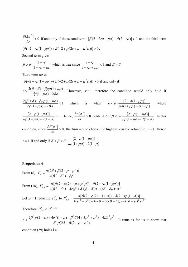
41

0][ *

>∂

∂r

E π if and only if the second term, 0)]2()22([ >−−+− ρδµρρβ rr and the third term

0))]2(2())1(2([ 2 >+++−+−+− ρµµρβµρρδ rr .

Second term gives

µρρρ

δβ+−

−⋅>

r

r

2

2 which is true since 1

2

2<

+−−

µρρρ

r

r and δβ >

Third term gives

0))]2(2())1(2([ 2 >+++−+−+− ρµµρβµρρδ rr if and only if

βρµρδρµρβµρδβ

2)1(

)1()(2

+−+−+

>r . However, 1≤r therefore the condition would only hold if

12)1(

)1()(2<

+−+−+βρµρδρµρβµρδβ

which is when )1(2)1(

)]1(2[

ρµρµρµρρ

δβ−−+

−−⋅< where

1)1(2)1(

)]1(2[>

−−+−−

ρµρµρµρρ

. Hence, 0][ *

>∂

∂r

E π holds if

)1(2)1(

)]1(2[

ρµρµρµρρ

δβδ−−+

−−⋅<< . In this

condition, since 0][ *

>∂

∂r

E π, the firm would choose the highest possible refund i.e. 1=r . Hence

1=r if and only if )1(2)1(

)]1(2[

ρµρµρµρρ

δβδ−−+

−−⋅<<

Proposition 6

From (6), 222

2*

)(4

))2(2(

βρδβρρβδα

−−−−+

=AP

From (18), 2222

2*

,)())((4)(4

))]1(2())2(2([

ρβµδρδβδβδβµρρδρµµρβα

−−−+−−−−+++−

=rr

rrP RA

Let 1=µ reducing *

,RAP to 2222

*

,)())((4)(4

))]1(2())12(2([

ρβδρδβδβδβρρδρρβα

−−−+−−−−+++−

=rr

rrP RA .

Therefore **

, ARA PP < iff

)2(2[

4)34()1(4)2(222

2232233

ρρβδρδρβδρρδβρδρρβ

−−+−++−+++

<r . It remains for us to show that

condition (29) holds i.e.

42

)2()(4

)2(23)(4

)2(2[

4)34()1(4)2(2232222

33222222

22

2232233

µρρδρµβδβρµρβδµρρµβρµβδβ

ρρβδρδρβδρρδβρδρρβ

++−−

++−−−>

−−+

−++−+++

which leads to

0]2)2(][)2([)2(

]4)4(][)2(][)][1(2[2222

222

>+−−−+−

−−−+−−+δρρβδρβρρδ

δρβδρρβδβρρδβ

which is true iff

ρδβ

+⋅>

2

1 which is true since 1

2

1<

+ ρ and δβ >

ρρ

δβ+

⋅>2

which is true since 12

<+ ρρ

and δβ >

24

2

ρδβ

−⋅> which is true under proposition 2

ρδ

β > (binding)

Proposition 7

(30) 0PPq AAA δβα +−=

(31) APPq 000 δβα +−=

and AAA qPqPqP ρπ 000 ++=

}{0, πPPA

Max will lead to

(32) β

βµρδδα2

)( 00 PP A

A

−++=

(33) )(2

)()1( 0

0

A

AA PP

µρδββµρδδµρα

−

−+++=

Solving for (32) and (33) results in

(34) )22(2)4(

))2((

0

22

0

222

0*

0

AAA

APδβµρδβµρδδδρµβ

µρβδδα−+−−−−

+++=

(35) )22(2)4(

))2()(1()1((

0

22

0

222

0*

AAA

AAP

δβµρδβµρδδδρµβδµρβµρµρδα

−+−−−−

++−++=

43

Substituting back to the demand functions will lead to

(36) )22(2)4(

)]())2(([

0

22

0

222

0

2

0*

AAA

AA

Aqδβµρδβµρδδδρµβ

δβµρβδδδµρββα

−+−−−−

+−−−++=

(37) and )22(2)4(

])1()2([

0

22

0

222

0

2

*

AAA

A

δβµρδβµρδδδρµβ

δδµρµρβαπ

−+−−−−

++++=

When 0→Aδ

0

2

0

222

0*

2)4(

])1()2)(1([

βµρδδρµβδµρµρµρβα

+−−

+++−=AP

0

2

0

222

0*

02)4(

])2([

βµρδδρµβδµρβα+−−++

=P

0

2

0

222

2

00

2*

2)4(

])1()2([

βµρδδρµβδµρβδµρβα

+−−

−−−+=Aq

0

2

0

222

2

0

22

0

222*

02)4(

])1()2([

βµρδδρµβµρδρµµρβδρµµρβα

+−−+−++−−

=q

When 00 →δ

A

APδµρβ

µρα−−

−=

)2(

)1(*

A

Pδµρβ

α−−

=)2(

*

0

A

Aqδµρβ

αβ−−

=)2(

*

A

Aqδµρβδµρβα

−−−−

=)2(

])1([*

0

The proof needs to show that 0

*

0

*

0 ==>

δδ AA PPA

Which is Aδµρβ

µραβµρδδρµβ

δµρµρµρβα−−

−>

+−−

+++−

)2(

)1(

2)4(

])1()2)(1([

0

2

0

222

0

44

Let 1=µ and assume that δδδ == 0A which would then lead to

])2(][)2(][)2([

)(2

0

*

0

*

0 δρβδρβδρβδδβραρ

δδ −++−−−−

=−== AA PP

A

and 00

*

0

*

0

>−== δδ AA PP

A

iff

ρδβ

+⋅>2

1 which is true since δβ >

ρδβ

−⋅>2

1 which is true since δβ >

and ρδ

β >

Similarly,

])2(][)2(][)2([

4

0

*

00

*

00 δρβδρβδρβ

αβρδδδ −++−−−

=−== A

PP

00

*

00

*

00

>−== A

PPδδ

which is true iff ρδ

β >

Proposition 8

From (38), assuming 1=µ

2

00

22

0

2

0

*

2)4(

)]1()2([

δρβδρβρδρβα

πδ −+−

+++=

=A

Aδρβα

πδ −−

== )2(

2

0

*

0

Assume that δδδ == 0A

and ])2(][)2(][)2([

])2([2

0

*

0

*

0 δρβδρβδρβδρβρδα

ππδδ −++−−−

++=−

== A

0> from proof of

proposition 7 above

45

REFERENCES

Alstrup, Jens et al. (1986), “Booking Policy for Flights with Two Types of Passengers,” European Journal of Operations Research, 27, 274-288. Badinelli, Ralph D. and Michael D. Olsen (1990), “Hotel Yield Management Using Optimal Decision Rules,” Journal of International Academy of Hospitality Research, November 26), 1, (accessed July 4, 2004), [available at http://scholar.lib.vt.edu/ejournals/JIAHR/issue1.html]. Bateson, John (1977), “Do We Need Service Marketing,” in Marketing Services: New Insights, Pierre Eiglier et al., eds. Cambridge: Marketing Science Institute. Belobaba, Peter P. (1989), “Application of a Probabilistic Decision Model to Airline Seat Inventory Control,” Operations Research, 37 (2), 183-197. Berstein, Peter L. (1996), Against the Gods: A Remarkable Story of Risk. New York: John Wiley and Sons. Bodily, Samuel E. and Lawrence R. Weatherford (1995), “Perishable-asset Revenue Management: Generic and Multiple-price Yield Management with Diversion,” Omega, International Journal of Management Science, 23 (2), 173-185. Chase Jr., Charles W. (1999), “Revenue Management: A Review,” Journal of Business Forecasting Methods and Systems, 18 (2), 2 and 28. Cook, Phillip J. and Daniel A. Graham (1977), “The Demand for Insurance and Protection: The Case of Irreplaceable Commodities,” Quarterly Journal of Economics, 91 (February), 143-154. Desiraju, Ramarao and Steven M. Shugan (1999), “Strategic Service Pricing and Yield Management,” Journal of Marketing, 63 (January), 44-56. Dixit, Avinash (1979), “A Model of Duopoly Suggesting a Theory of Entry Barriers,” Bell Journal of Economics, Vol. 10, No. 1, pp20-32 Edgett, Scott and Stephen Parkinson (1993), “Marketing for Service Industries - A Review,” The Service Industries Journal, 13(3), 19. Fishburn, Peter C. (1974), “On the Foundations of Decision Making under Uncertainty,” in Essays on Economic Behavior under Uncertainty, M.Balch, D. McFadden, S. Wu, eds. North Holland Publishing Co. Gallouj, Faiz (2002), Innovation in the Service Economy: The New Wealth of Nations, Edward Elgar Publishing. Hersh, Marvin and Shaul P. Ladany (1978), “Optimal Seat Allocation for Flights with One Intermediate Stop,” Computers and Operations Research, 5, 31-37. Ingene, Charles A. and Mark E. Parry (1995), “Channel Coordination When Retailers Compete,” Marketing Science, 14 (4), 360-377. Jagpal, Sharan (1998), Marketing Strategy and Uncertainty, USA: Oxford University Press. Johnson, E. (1970), “The Selling of Services” in Handbook of Modern Marketing, Victor P Buell. New York: McGraw-Hill. Karni, Edi (1983), “Risk Aversion for State-Dependent Utility Functions: Measurement and Applications,” International Economic Review, 24 (3) (October), 637-647. Kimes, Sheryl E. (1989), “Yield Management: A Tool for Capacity-Constrained Service Firms,” Journal of Operations Management, 8 (4) (October), 348-363. Lee, Khai Sheang and Irene C.L. Ng (2001), “Advanced Sale of Service Capacities: A Theoretical Analysis of The Impact of Price Sensitivity on Pricing and Capacity Allocations,” Journal of Business Research, 54 (3), 219-225.

46

Levine, Michael E. (1987), “Airline Competition in Deregulated Markets: Theory, Firm Strategy and Public Policy,” Yale Journal on Regulation, 4, 393-494. Lieberman, Warren H. (1993), “Debunking the Myths of Yield Management,” Cornell Hotel and Restaurant Administration Quarterly, (February), 34-41. Lieberman, Varda and Uri Yechiali (1978), “On the Hotel Overbooking Problem: An Inventory Problem with Stochastic Cancellations,” Management Science, 24, 1117-1126. McGuire, Timothy W. and Staelin, Richard (1983), “An Industry Equilibrium Analysis of Downstream Vertical Integration,” Marketing Science, 2 (2) (Spring), 161-191. Nagle, Thomas T, Reed K. Holden, Reed Holden (2002), The Strategy and Tactics of Pricing: A Guide to Profitable Decision Making, 3rd Edition, Prentice Hall. Pfeifer, Philip E. (1989), “The Airline Discount Fare Allocation Problem,” Decision Sciences, 20, 149-157. Png, Ivan P.L. (1989), “Reservations: Customer Insurance in the Marketing of Capacity,” Marketing Science, 8 (3) (Summer), 248-264. ---- 1991,“Most-Favored-Customer Protection versus Price Discrimination over Time,” Journal of Political Economy, 99(5), 1010-1028. Rathmell, John (1966), “What is Meant by Services?”, Journal of Marketing, 30(4), 32-36. Regan, W(1963), “The Service Revolution,” Journal of Marketing, 27(3), 57-62. Relihan III, Walter J. (1989), “The Yield Management Approach to Hotel-Room Pricing,” Cornell Hotel and Restaurant Administration Quarterly, (May), 40-45. Rothstein, Marvin (1971), “An Airline Overbooking Model,” Transportation Science, 5, 180-192. ---- 1974, “Hotel Overbooking as a Markovian Sequential Decision Process,” Decision Sciences, 5,389-

394. ---- 1985, “Operations Research and the Airline Overbooking Problem,” Operations Research, 33 (2),

237-248. Shugan, Steven M. and Xie, Jinhong (2000), “Advance pricing of services and other implications of separating purchase and consumption,” Journal of Service Research, 2 (3), 227-239. Nirvikar Singh & Xavier Vives, (1984), "Price and Quantity Competition in a DifferentiatedDuopoly," RAND Journal of Economics, 15 (4), pp. 546-554. Thompson, H.R. (1961), “Statistical Problems in Airline Reservation Control,” Operational Research Quarterly, 12, 167-185. Toh, Rex (1979), “Airline Revenue Yield Protection: Joint Reservation Control Over Full and Discount Fare Sales,” Transportation Journal, (Winter), 74-80. ---- 1985, “An Inventory Depletion Overbooking Model For the Hotel Industry,” Journal of Travel

Research, (Spring), 24-30. Xie, Jinhong and Shugan, Steven M. (2001), “Electronic Tickets, Smart Cards and Online Prepayments: When and How to Advance Sell,” Marketing Science, 20(3) Summer, 219-243.