The Price Elasticity of the Demand for Residential Land

Joseph Gyourkoa and Richard Voithb

First Draft: March 31, 1998Revised: February 9, 2000

aReal Estate and Finance Departments, The Wharton School, University of PennsylvaniabResearch Department, Federal Reserve Bank of Philadelphia

The authors gratefully acknowledge funding for this research from the Lincoln Institute of Land Policyand the Research Sponsors Program of the Zell/Lurie Real Estate Center at The Wharton School,University of Pennsylvania. This paper does not necessarily reflect the views of the Federal ReserveBank of Philadelphia or of the Federal Reserve System.

Abstract

The price elasticity of demand for residential land is estimated using a suburban Philadelphia

data base that includes appropriate instruments to deal with the simultaneity issues raised by Bartik

(1987) and Epple (1987) when estimating demand functions for bundled goods. We find that the price

elasticity is fairly high, -1.6 in our preferred specification, and that OLS estimates of the price elasticity

(based on estimates of inverse demand schedules) are biased upward substantially as predicted by

Bartik (1987) and Epple (1987). Because the demand for residential land is so elastic, it has important

implications for a host of urban issues and the emerging ‘smart growth’ debate. In particular, ‘smart

growth’ policies–most of which would raise the price of residential land–could lead to much increased

residential densities. The high elasticity also implies that other policies, such as the federal tax treatment

of housing which lower the relative price of land primarily for higher income households, could increase

the incentives for residential sorting.

-1-

I. Introduction

A host of metropolitan issues ranging from central city decline to suburban traffic congestion

and the perception of disappearing green space are hotly debated in academia and the press. These

issues tend to be covered under the rubric of ‘smart growth’ initiatives which are being taken up by

politicians ranging from local zoning boards to Vice President Al Gore. The emerging ‘smart growth’

debate is intimately related to society’s adoption of less dense land usage patterns. At least to date, the

discussion does not appear to recognize that the impact of any policy designed to alter land use patterns

is dependent, at least in part, upon the nature of the demand for land.

Analysis of the demand for land has a long tradition and received increased scrutiny in urban

economics when the now standard Mills-Muth-Alonso city model was developed in the 1960s. Muth

(1964, 1969, 1971) in particular, provided a simplified framework in which to evaluate the demand for

residential land. In contrast to Alonso (1964), who viewed residential land as a good over which

consumers held preferences, Muth argued that the demand for residential land was derived solely from

its role as a factor of production in housing. Muth’s empirical estimates of the derived demand for

residential land in his 1971 article helped establish a concensus that the price elasticity of demand for

land was in the -0.8 to -1.0 range. Subsequent advances in applied econometric theory by Bartik

(1987) and Epple (1987) imply that these estimates are biased downward. The primary contribution of

this paper is to provide an unbiased estimate of the price elasticity. Our findings confirm Bartik’s and

Epple’s insights and bring new evidence to bear on the nature of the demand for residential land.

Because residential land is typically bundled with housing, its price is seldom directly observed.

Although residential land prices can be estimated using standard hedonic techniques, the bundled aspect

-2-

of residential land introduces additional econometric issues that make estimating its price elasticity of

demand a very difficult task. Bartik (1987) and Epple (1987) showed that the nonlinearity of the

underlying hedonic price function relating house value to a trait bundle effectively allows consumers to

choose both quantities and marginal prices of all traits--including lot size. Under these circumstances,

ordinary least squares (OLS) estimation of an inverse (regular) demand schedule is likely to result in an

upwardly (downwardly) biased price elasticity. Moreover, identification of the underlying demand

function places onerous requirements on the data that seldom are satisfied. First, repeated observations

on the market of interest are needed. Second, the distribution of preferences must not change across

the repeated observations of the market. Third, the data must include instruments that shift the

household’s budget constraint but which are uncorrelated with unobserved tastes that could be

influencing the consumed trait set. If these conditions are satisfied, consistent estimates of the

parameters of the demand function can be obtained using the two-stage least squares (2SLS),

instrumental variable (IV) procedure described by Bartik (1987) and Epple (1987).

Fortunately, we are able to address these issues with a unique data set on house transactions

from Montgomery County, PA. This data base includes virtually all single family housing transactions

spanning a nearly 30-year period from 1970-1997 in the most populous suburban county in the

Philadelphia metropolitan area. All observations have been geocoded so that street addresses are

known in addition to a wealth of structural trait data.

Our identification strategy treats each year as a single observation on the market and makes the

assumption that the distribution of preferences does not change across years–at least in ways that we

cannot control for. The results confirm Bartik’s (1987) and Epple’s (1987) conclusion that OLS

-3-

estimates of price elasticities arising from inverse demand schedules are biased upward. In our

preferred specification, the OLS-based price elasticity of about -2.5 is about 50 percent higher than the

-1.6 figure resulting from the 2SLS estimation.

Our finding that the price elasticity of demand for residential land is relatively high is important

for two reasons. First, it has powerful implications for how various public policies can affect urban

form. Simply put, if the price elasticity is high, policies that affect land price can materially affect

residential density and in some cases residential sorting by income. Second, in contrast to Muth’s

(1964, 1969, 1971) view that the demand for residential land can be described solely as a derived

demand based on its role as a factor of production in housing, our findings suggest there is an

independent demand for land as was postulated by Alonso (1964).

The remainder of the paper is organized as follows. The next section outlines the econometric

issues first raised by Bartik (1987) and Epple (1987) involved in estimating the price elasticity of

demand for a single trait such as residential lot size. Section III then describes the Montgomery

County, PA, data base in more detail. This is followed with Section IV’s presentation of the

specifications estimated and a discussion of key results. Section V outlines the implications of our

findings for how policy that changes land prices might impact urban form and for the nature of the

demand for residential land. A brief summary concludes the paper.

II. Econometric Issues

Using hedonic techniques to estimate market prices of individual traits in bundled goods is

standard fare in empirical studies of housing markets, but estimates of the underlying demand functions

-4-

for these traits are rare. Determining the price elasticity of demand for a single trait such as residential

lot size is fraught with more than the typical identification problems involved in any situation in which

demand (or supply) must be estimated. Bartik (1987) and Epple (1987) pointed out the unique

identification problems in their critique of Rosen’s (1974) suggested methodology for estimating the

supply and demand schedules for bundled traits.

Rosen (1974) analyzed the issue as a standard identification problem and suggested the

following two-step procedure for estimating the supply and demand functions for traits of bundled

goods. First, compute individual equilibrium trait prices based on estimates of a hedonic price function

such as that for housing shown in equation (1):

(1) Vi = f(Zik; $k ) + ,i,

where: Vi is the observed value of house i;

Zik is a vector of housing traits;

$k is vector of parameters;

,i is the random error term.

The market price of a trait in the bundle such as residential land, l, is given by pil = MVi/MZil. Note that

if the hedonic price function is nonlinear, the price of residential land will vary across houses.

The second step is to estimate an inverse demand or marginal bid function using the trait price

as the dependent variable:

(2) pil = MVi/MZil = h( Zil, Ei, Di; (1, (2, (3) + µi,

where: Zil, is the amount of residential land;

-5-

Ei is non-housing expenditure;

Di is a vector demand shifters;

(j are coefficient vectors; and

µi is an error term.

A companion marginal offer function would be estimated along with (2) and would contain individual

supplier traits (Si). Rosen (1974) suggested that two-stage least squares (2SLS) be employed, with the

supplier traits being appropriate instruments for the endogenous Z and E vectors in the marginal bid

function.

Bartik (1987) and Epple (1987) pointed out that the most difficult issue in estimating individual

trait demand parameters does not lie in traditional supply-demand interaction, as no individual

consumer’s behavior can affect suppliers because a single consumer cannot influence the hedonic price

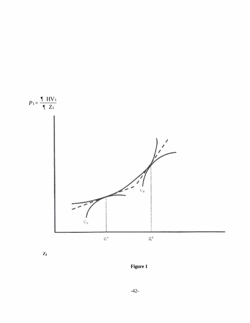
function itself. Rather, the crux of the problem lies in the nonlinearity of the hedonic price function

which implies that consumers simultaneously choose both quantity and marginal price of the housing

trait. Epple (1987) illustrated this with a graph similar to that in Figure 1 which has the hedonic price of

the trait on the vertical axis and the quantity of the trait on the horizontal axis. Even though the

distribution of supply is exogenously given in this example, the nonlinearity of the hedonic price function

means that the price changes with any quantity chosen as indicated by the two tangencies in the figure.

Hence, a choice of price necessarily implies a choice of quantity (and vice versa). In this situation,

OLS estimates of the parameters of the inverse demand function given in equation (2) imply a greater

1The problem essentially is one of omitted variables. Unobserved individual tastes that arepositively correlated with both price and quantity are omitted from the estimation, causing the estimatedresponses of marginal bids to the quantity consumed to be biased upward (toward zero in this case). Stated differently, a household with a strong preference for a given trait in the Z vector will choosemore of it and be willing to pay a higher price for it (cet. par.). Note that if equation (2) were linear,the price elasticity would be 0 = (1/(1)pl /Zl, and since (1 is biased upward toward zero, it implies anestimated elasticity greater than the true price elasticity.

-6-

price elasticity than the true price elasticity.1 Conversely, OLS estimates of a regular demand function

in would yield parameters that imply a result less than the true price elasticity.

The solution to this problem is an instrumental variables estimation, but of a different type than

that employed for the standard supply-demand identification problem. Appropriate instruments are

those that exogenously shift the household budget constraint yet are uncorrelated with unobserved

tastes. The reason is that a shift in the budget constraint will be correlated with the observed Z (and E)

vectors, yet uncorrelated with tastes. Thus, it deals with the underlying omitted variables problem

because it allows estimation of the response to changes in quantity holding constant the unobserved

tastes. Bartik and Epple recommend two classes of factors that can shift the budget constraint

exogenously as candidate instruments. One is income or wealth. The other is the set of variables that

shift the hedonic price function, assuming that average tastes do not change across those shifts. This

assumption is very important because of what it requires of the data. In particular, it suggests that

multiple observations on the market that satisfy two conditions are needed. First, the distribution of

tastes must be unchanged across observations on the market. And, second there must be forces that

shift individuals’ budget constraints across observations on the market.

We are fortunate to have a unique data base to deal with both requirements. Our data are from

2Because the 2000 census has not been taken, we do not have more recent data but we expectmore of the same in terms of the county’s demographics. Note that the assumption the distribution of

-7-

tax assessment files containing observations on transactions of single family detached homes in

Montgomery County, PA, over the period 1970-1997. We treat sales in each year as an observation

on the market for homes, with the maintained hypothesis being that the distribution of preferences in the

county does not change over time (or at least does not change in a way that we cannot control for in the

estimation).

Given the importance of the assumption, some discussion of it is useful. Across Montgomery

County there are small lots and big lots, and preferences certainly differ over this trait. However, the

key issue for us is that the county-wide distribution of preferences over time does not change

much–again, in ways we cannot control for. A look at key demographics that are known to influence

the rent-own decision and to affect the demand for housing suggests great stability over time in

Montgomery County. For example, even though the population in the county has risen by 55,000 from

623,799 in 1970 to 678,111 in 1990, the fraction of males has changed by only 0.1 percent. The

percentage of adults (i.e., those at least 18 years of age) has barely risen–from 66.3 percent in 1970 to

68.8 percent in 1990. The median age was 31 in 1970 and 33 in 1990. The county was and still is

overwhelmingly white, being 96.1 percent white in 1970 and 91.5 percent white in 1990. And, in 1990

Montgomery County’s mean and median income still was the highest among all suburban Philadelphia

counties. Thus, in many ways the demographic make-up of the county looks the same in 1990 as it did

in 1970, providing support for our assumption that the distribution of preferences is not changing much

over time.2

tastes is unchanged across observations on the market would be much more tenuous if we tookindividual suburbs as our markets. In that case, hedonic prices would be estimated for each locality,with the assumption being that the preference distribution is the same across localities. It strikes us thatthe distribution well could be different in a large lot suburb on the urban fringe versus a small lot, inner-ring suburb. Hence, our choice of sales throughout the county in a given year as an observation on themarket.

-8-

Given our assumption that an annual cross section of sales constitutes one observation on the

market, hedonic regressions of the type illustrated in equation (1) are estimated by year to determine

annual market prices of a square foot of lot size (pl). Were we not concerned with the price of

residential land and residential lot size being simultaneously determined, an inverse demand function (or

marginal bid) could be estimated via OLS with the price of land, pil, regressed on the quantity of land,

Zil , and other appropriate terms such as demand shifters (denoted D) and non-housing expenditures

(E). Because of the simultaneity problem, however, we must estimate the marginal bid function via

2SLS in which Zil and Ei are instrumented for by a set of variables that shift the household’s budget

constraint without being correlated with tastes. Thus, the specification we estimate via 2SLS is of the

form described by equation (3),

(3) pil,t = h( ^Zil,t, ^Eit, Dit; "1, "2, "3 ) + >il,t

where "j are coefficient vectors;

>it is the error term; and

^Zil,t, and ^Eit are instruments generated from equations (4) and (5) below.

(4) ^Zil,t = gz (Dit, Sit; .D, .S) + <it

(5) ^Eit = gE (Dit, Sit; 2D,2S) + Lit

where: Sit is a vector of variables that shift supply or both supply and demand;

3While our data begin in 1970, lagging in the regression analysis reported below results in theloss of the first two years of data. To maintain consistency with the regression analysis, we reportsummary statistics for the 1972-1997 period throughout the paper.

-9-

.k and 2k are parameters of the instrument equations; and

<it and Lit are the error terms and all other terms are defined as above.

The price elasticity of most interest to us can be computed from the "1 coefficient. Before getting to the

specifics of the estimation and the results, the next section more fully describes the data employed in

estimating equations (1) as well as instrument equations (4) and (5).

III. Data

The core data base was created from tax assessment files for Montgomery County, PA, the

most populous suburban county adjacent to the city of Philadelphia. The data begin in 1970 and end in

1997. Montgomery County extends from the Philadelphia border to the metropolitan fringe. All

observations are geocoded so that precise location within the county is known, allowing matching of

observations to census tracts and local jurisdictions. There are 53 such jurisdictions in our sample. The

tax assessment data cover all properties in the county and include information on a variety of housing

characteristics in addition to sales price. We focus our attention on the nearly 100,000 observations on

sales transactions of single family homes.

Housing Traits, Neighborhood Characteristics and House Prices

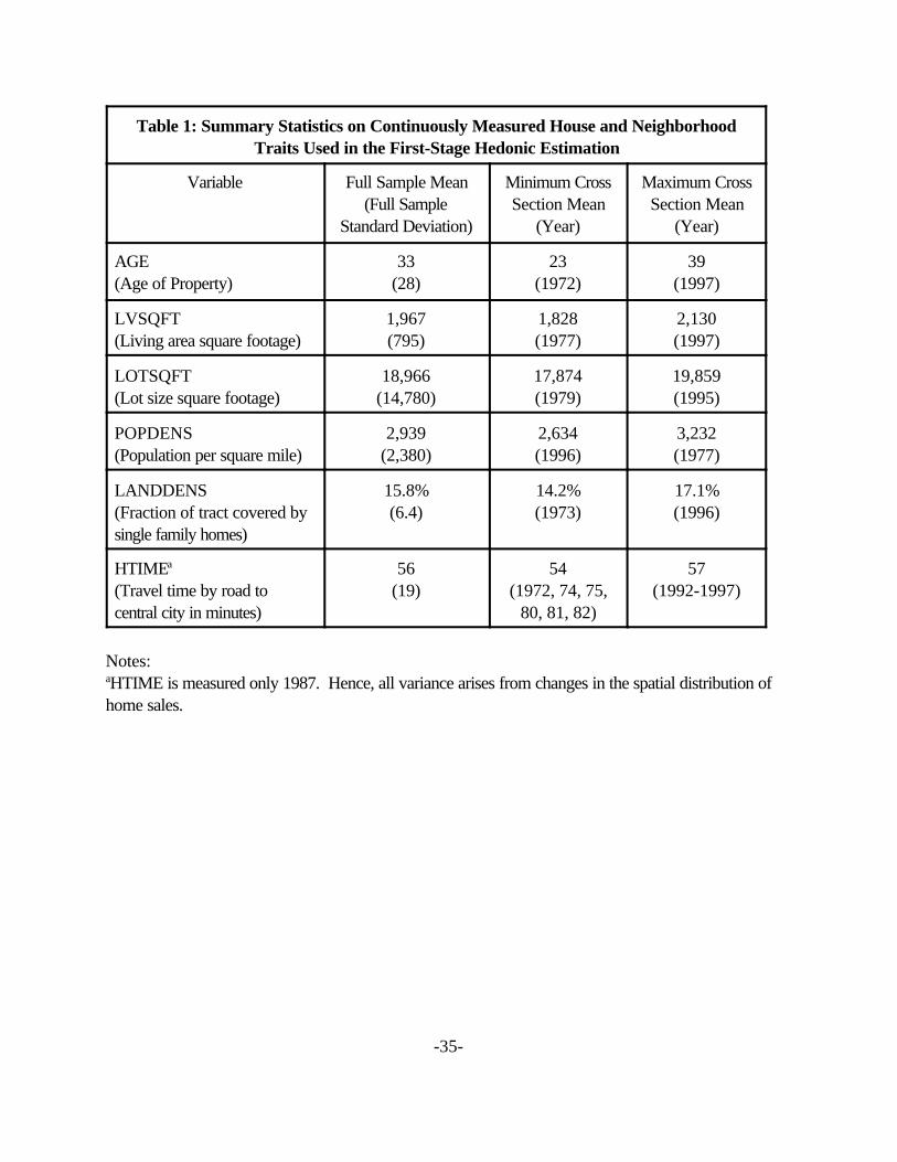
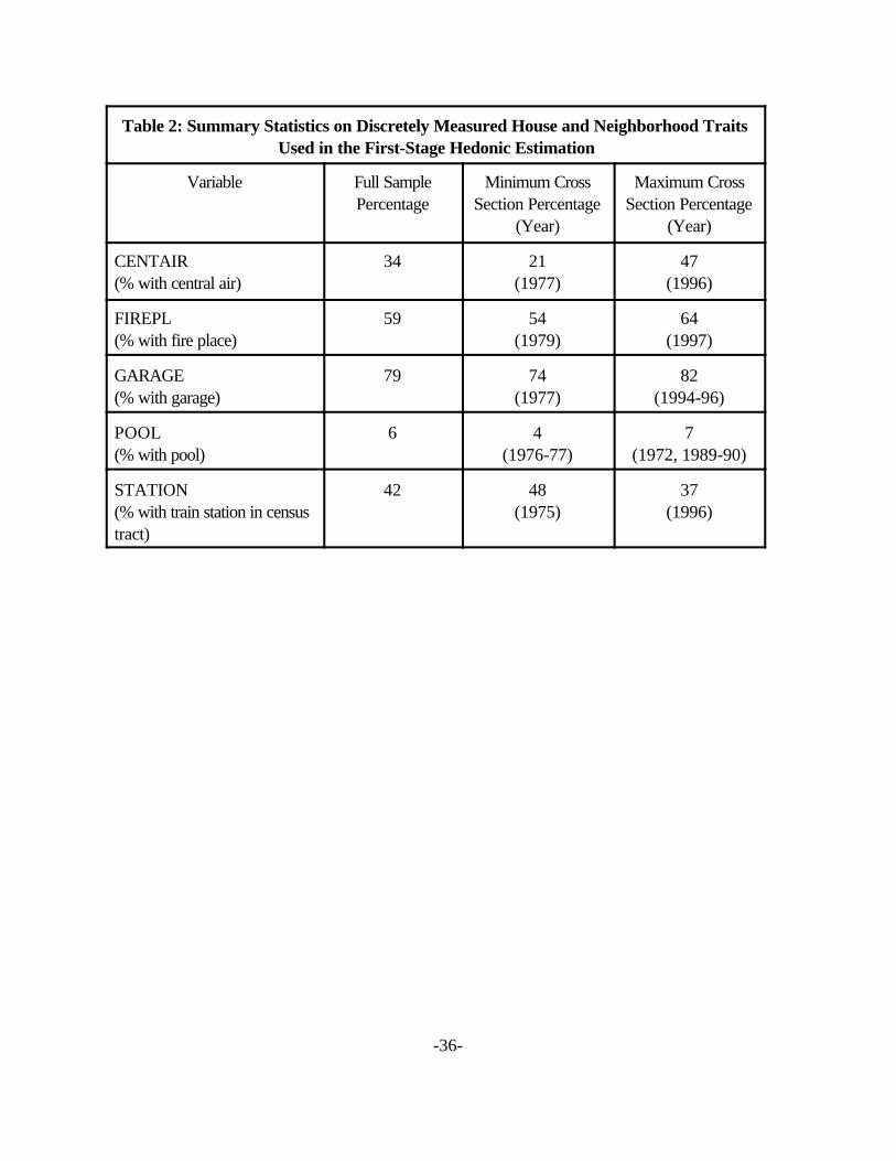
Tables 1 and 2 report summary statistics on structural traits and neighborhood characteristics

used in the hedonic equation. Full sample means over 1972-1997 are reported along with minimum

and maximum values across all cross sections.3

4Median values obviously are lower, with the median lot size in 1972 and 1997 being just under15,000 square feet. Hence, the median sale was on a house with about one-third of an acre of land.

-10-

The values of the housing traits themselves are quite stable over time. Even with building on the

suburban fringe, Montgomery County housing has not changed all that much over time, with average

housing quality being fairly high at the beginning of the sample. The maximum living area (LVSQFT) of

2,130ft2 in 1997 is only 16 percent higher than the minimum of 1,828ft2 in 1977. Lot size (LOTSQFT)

also has increased only slightly on average, with the maximum mean size of 19,859ft2 in 1995 versus a

minimum mean size of 17,874ft2 earlier in 1979.4 Central air conditioning (CENTAIR) is more

prevalent over time, increasing from being in only 21 percent of sold homes in 1977 to 47 percent in

1996. However, the biggest change is in the age of the stock (AGE). It is getting older. The mean age

was 21 in 1977, while in 1997 the mean age of a house that sold was 47. The vast majority of sales in

Montgomery County clearly are not new homes constructed on the urban fringe. In addition to the

housing traits listed above, we also have data on a number of other features of the properties, including

a dummy variables for the presence of a garage (GARAGE), a pool (POOL), or fireplace (FIREPL).

Neighborhood characteristics also are quite stable over time. The biggest change is in

population density of the census tract where sales are occurring (POPDENS), which has fallen nearly

20 percent from its peak in 1977. This undoubtedly reflects the expansion to the northern and western

parts of the county which are on the urban fringe. The fraction of a census tract covered by single

family housing (LANDDENS) is between 14 and 17 percent, depending upon the year. In addition to

density variables, we also have data that measure accessibility to center city Philadelphia. Commute

time to Philadelphia’s central business district (HTIME) is very stable because it is not measured

-11-

annually, but only at one point in time (1987). Changes in that variable’s mean arise because the spatial

distribution of sales varies across years. Commuter train access to Philadelphia’s CBD is measured by

a dummy variable for the presence of a train station in the neighborhood (STATION). In most years,

forty percent or more of homes in our sample are in communities with train stations connecting to the

central city of Philadelphia.

Mean and median sales prices by year are reported in Figure 2. This and all other monetary

values always are in 1990 dollars. The table depicts the large changes in real prices that have buffeted

the Philadelphia market in general and Montgomery County in particular. For example, there was an

80% real increase in mean price from the 1982 recession to the peak in 1988-89. Since then mean

home prices have trended down over 15%. Median prices move by almost as much. Both mean and

median figures are well above national averages for existing homes as reported by the National

Association of Realtors, reflecting the above average quality of the county’s housing stock.

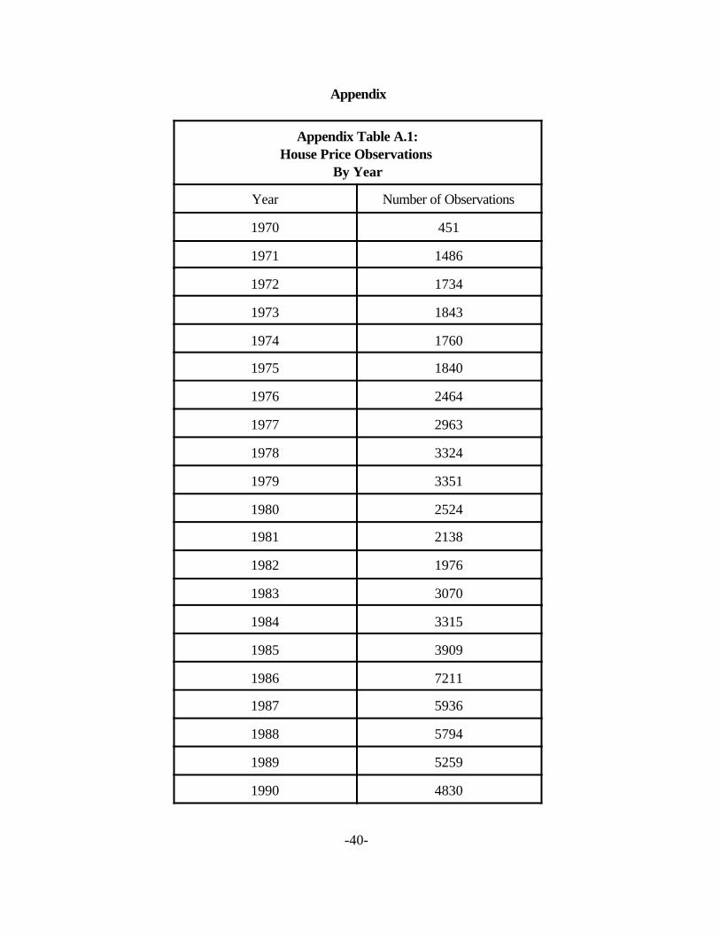
Finally, the number of observations each year are reported in the Appendix. Observations

generally increase over time, although there is a clear cyclical pattern to the number of sales. The

fewest number of observations in any year is 1,532 in 1972 versus a maximum number of 7,063 in

1986.

Supply and Demand Shifters: Instruments for Lot Size and Non-Housing Expenditure

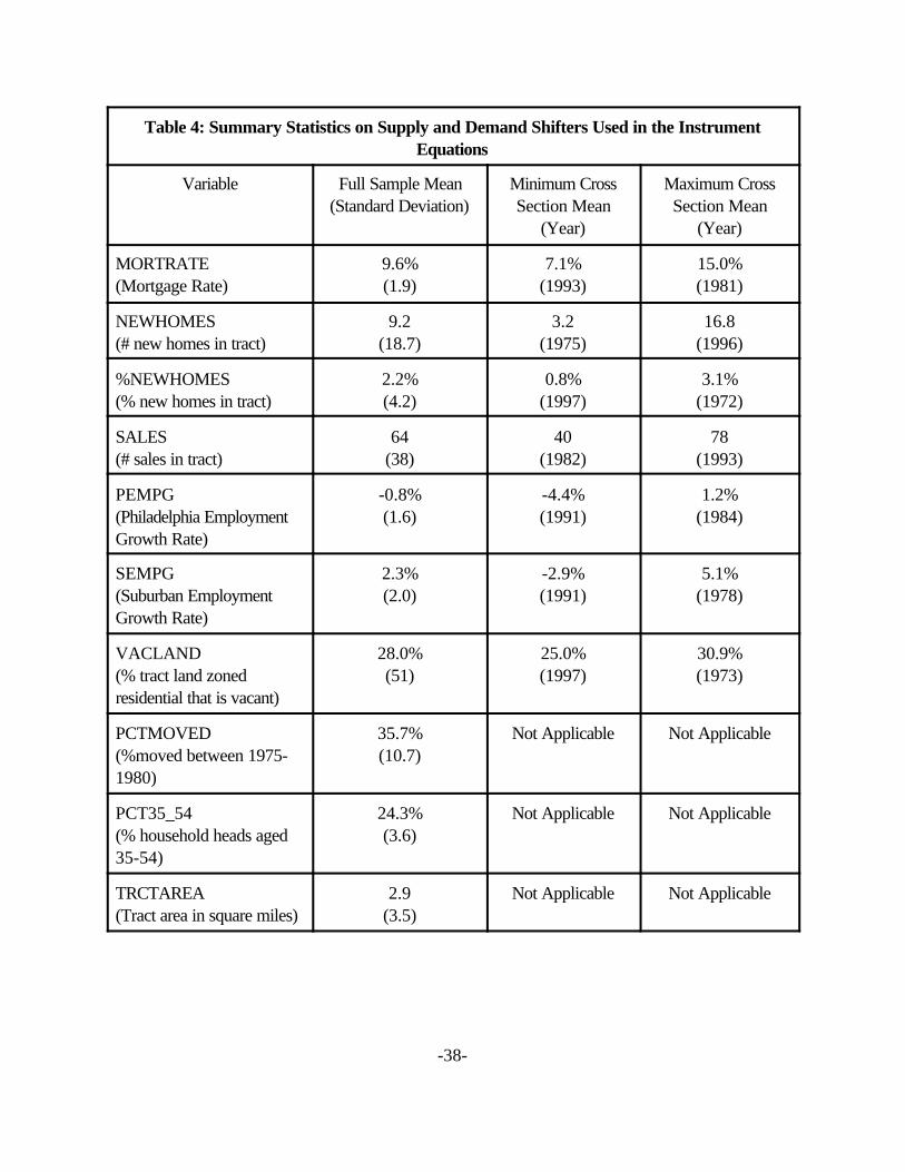
Table 3 reports the full list of variables used as instruments for lotsize (Zl) and non-housing

expenditures (E) in the 2SLS demand estimation. Summary statistics on the variables are reported in

Table 4. Recall that candidate instruments are those which shift the household’s budget constraint

without being correlated with tastes. It is noteworthy that the restriction instruments not be correlated

-12-

with tastes effectively rules out a strategy of using lagged values of regressors as instruments. It also

prevents use of previous sale prices, which is unfortunate because there are many repeat sales

observations in our data. The previous sales price is likely to incorporate information about the tastes

of the current occupant.

Fortunately, we are able to amass a considerable number of demand and supply shifters that

reasonably could be thought to shift the budget constraint exogenously. Those variables likely to work

through supply are listed in the top panel of Table 3. Supply shifters include a variety of new

construction, tract size, and vacant land measures that capture actual and potential changes in housing

activity across individual census tracts. These variables reflect the number of new homes built in the

tract each year (NEWHOMES), how extensive is new construction as measured by the fraction of

homes in the tract that are new in any given year (%NEWHOMES), census tract size in square miles

(TRCTAREA), and the amount of vacant land available for residential development in each year

(VACLAND). Except for TRCTAREA which is measured only in 1980, each of these variables varies

over time.

Table 4 shows that the mean number of new homes per year in a tract over the full sample is

9.2. This variable is cyclical as indicated by the low of 3.2 in 1975 and the high of 16.8 in 1996. New

homes as a fraction of all homes in the tract averages 2.2 percent over the sample, with the annual

means varying from one to three percent. The mean tract size (TRCTAREA) is 2.9 square miles.

While there is no intertemporal variance in this variable, there is considerable variance across tracts as

the standard deviation is 3.5 square miles. The mean fraction of vacant land available for residential

development (VACLAND) does not vary much over time, averaging from 25 to 30 percent depending

5The suburban growth rate is based on employment growth in all four Pennsylvania suburbancounties of Philadelphia--Bucks, Chester, Delaware, and Montgomery.

-13-

upon the year. As with tract size, there is much more cross sectional variance.

The instruments likely to work only through the demand side, listed in the middle panel of Table

3, are employment growth in the city of Philadelphia (PEMPG) and employment growth in the suburbs

of Philadelphia (SEMPG). Employment growth is likely to increase housing demand in communities in

close proximity to the location of the employment growth. Over the full sample period, the city’s

employment growth averaged just under -1% per year, with the suburban growth exceeding 2% per

year on average.5 Table 4 shows that there is substantial variance in these data over time. We use two

annual lags of these variables and interact them with locality dummies for the 53 municipalities in our

sample. Interaction terms are included because the demand-side impact of city and suburban growth

can shift the budget constraint differently in different parts of the metropolitan area. Using these data,

Voith (1999) has shown that the housing market impacts of city employment growth differs markedly

for that of suburban employment growth, and that the impacts of both city and suburban growth vary

across location withing the county.

A final set of instruments includes demographic and financial variables whose impact on the

budget constraint could work through both supply and demand. The thirty year mortgage interest rate

(MORTRATE), for example, is likely to reflect both shifts in supplier and demander costs and hence

shifts the budget constraint. The average loan rate for the sample period is 9.6 percent, although this

varies widely over time as our series spans the high inflation late 1970s and early 1980s as well as the

low inflation 1990s. The mortgage rate also is interacted with municipality dummies to capture

6These two variables are highly correlated with the analogous figures from the 1990 census. The mean fraction of households that moved between 1985 and 1990 is 37 percent, or two pointshigher than found a decade earlier. The fraction of household heads between the ages of 35 and 54also is marginally higher in 1990.

-14-

differences in how the budget constraint shifts across location.

Demographic variables include a mobility measure, PCTMOVED, which reflects the fraction of

households that moved between 1975 and 1980 and PCT35_54 which measures the fraction of

household heads between the ages of 35 and 54. This age range spans the prime home owning years

of the life cycle. These variables are computed from the STF3 files of the 1980 census and have no

intertemporal variance. Mobility is relatively high as indicated by the fact that over 35 percent of

households in our tracts had a different residence in 1980 versus 1975. Nearly a quarter of household

heads in these tracts are between 35 and 54 years of age.6 In addition to the mobility measures, we

also have total sales in the tract each year (HOMESALE), which captures changes in the actual level of

transactions over time. Sales of homes in a tract also are cyclical. For example, it bottoms out at 40

homes per tract during the 1982 recession before increasing to 78 in 1993.

Non-Housing Expenditures

While our data are very strong in terms of housing, location controls, and potential supply and

demand shifters, the Montgomery County tax assessment files do not contain detailed information on

household income. The only income data in the files is mean income at the tract level for 1980.

Consequently, we use data from the American Housing Surveys (AHS) in conjunction with this figure

to impute income at the household level. Using the observations on houses in the Philadelphia suburbs

7We use every available annual survey plus all special metropolitan surveys of the Philadelphiametropolitan area (done approximately every 4-6 years) in this effort.

-15-

that can be identified from the AHS7, we begin by defining household income (y) in deviation from mean

form as shown in equation (6),

(6) yi = ln Yi - ln Y,

where Yi is the income for household i and Y is the sample mean across all years. Income in deviation

from mean form then is regressed on a set of housing traits (xi=Xi-X, also in deviation from mean form)

common to both the Montgomery County and AHS data sets and a set of time dummies as shown in

equation (7),

(7) yi = xi*1 + TimeDummies*2 + >i,

where > is an error term.

The coefficient vectors *1 and *2 are then used to impute household incomes in the

Montgomery County data base. This is done in a way that incorporates the mean tract income

information that is available. For the purposes of exposition, denote that tract mean value (which does

not vary over time) as Yc. An increment to that value is imputed, introducing time series and cross

section variance from the AHS. This increment, denoted yi,m, is imputed via the following equation,

(8) yi,m = xi,m*1 + TimeDummies *2,

where xi,m represents a housing trait vector in deviation from mean form analogous to that in equation

8The 7% rate is arbitrary in the sense it is not estimated, but it is within the range reported in theliterature. We have experimented with small changes about this number. No result reported below isaffected in any meaningful way by this.

-16-

(7), with *1 and *2 being the coefficient vectors estimated in equation (7) .

Imputed household income for the Montgomery County observations then is ^Yi = Yc + yi,m.

Finally, non-housing expenditures (denoted E, which is what is required by theory for the demand

estimation) is computed using a capitalization rate c to convert house values into service flows as in

equation (9),

(9) Ei = Yi - cV,

where V is house value (the sales price in the Montgomery County data) and the cap rate is assumed to

be 7%.8 The end result is a mean non-housing expenditure value of E=$38,885 with a standard

deviation about that mean of $17,321.

IV. Specifications and Results

Hedonic Price Functions

The first task in determining the price elasticity of the demand for residential lot size is to

estimate the hedonic price of an added square foot of lot size via a specification as in equation (1).

Because we want to estimate the price of a square foot of a generic lot, our hedonic specification

contains housing traits and neighborhood characteristics, including controls for density and location

within the metropolitan area. The structural trait and neighborhood characteristics used include those

listed above in Tables 1 and 2. Three of the housing traits were entered in quadratic form: age (AGE,

9A full grid search was conducted because experimentation showed that results were sensitiveto starting values. We approximated the likelihood and mapped out the surface for all possiblecombinations of the transformation parameters 8 and (say) 2 for the right-hand side variables. Thelikelihood proved to be very flat throughout the full range of 2 values. Hence, we do not transform theindependent variables. The likelihood proved much more sensitive to the value of 8. The resultsreported below are from an estimation that uses as a starting point for the Box-Cox estimation the 8value from our grid search that maximized the likelihood.

-17-

AGE2), living area (LIVAREA, LIVAREA2), and lotsize (LOTSIZE, LOTSIZE2).

The specification of the hedonic employs a Box-Cox transformation of the dependent variable

(real house price) as illustrated in equation (10).

(10) (Vi8 -1)/8 = Zi$ + ei,

where 8 is the transformation parameter. This model is estimated on each annual cross section,

although the time subscript is dropped for convenience sake.

We arrived at this specification after a full grid search of possible Box-Cox parameter values

showed that the likelihood function was not sensitive to transformation of the right-hand side variables.9

The transformation parameter is always significantly greater than zero and averages 0.316, with the vast

majority of estimated values falling between 0.25 and 0.40. Thus, the Box-Cox parameters indicate

that the data tend to favor something much closer to the semi-log functional form traditional in many

housing studies over a linear functional form. That said, the data confidently reject the null that 8=0 in

each cross section.

The equilibrium price of a square foot of lot can be calculated from (10) as

(11) pil = MVi/MNil = $l V^

i(1-8),

with the partial derivative evaluated using coefficients estimated in equation (10) and each observation’s

10The actual computation was slightly more complicated because the house value, lot size andlot size squared were scaled to facilitate the estimation.

11We experimented with a series of alternative specifications of equation (10). For example,allowing lot size to enter in cubic form has little impact on the results. If we do not perform a Box-Coxtransformation of house price and estimate a traditional semi-log functional form, land prices are slightlyhigher on average. There also are more negative lot prices from that estimation. However, this has littleimpact on the 2SLS results and the price elasticity of demand estimates discussed in the next section.

-18-

predicted value, V^ i from the same equation.10 The plot in Figure 3 shows that the price of a square foot

of land varies considerably over time, but is without a discernable long term trend. The wide variance is

not unexpected as land effectively is the residual claimant on house value. Casual observation of the

time series shows that land prices fall substantially at the beginning of recessions and depressed housing

markets and rise markedly just after the economic upturn begins. Land prices peaked in Montgomery

County in the late 1980s, reaching $1.51/ft2 in 1988. Since then prices have trended down roughly 30

percent in real terms, although the last year of data shows a marked upturn in price that the popular

press suggests has continued into 1998 and 1999. As a percentage of house value, the prices in Figure

3 hover around 15 percent of mean house value in most years. In 1972, the $1.03 price per square

foot implies land constitutes 17 percent of mean house value that year assuming the mean lot size of

19,856ft2 for that year. The low is reached in 1992 when the $0.89 per square foot price implies land

is only 10 percent of the mean house value that year.11

Estimating the Price Elasticity of Demand Via 2SLS

Using the estimate of pl derived from equation (10)’s hedonic specification, an inverse demand

function of the type illustrated above in equation (3) is estimated The results presented below are from

a specification in which lot price (pl), lot size (Zl,), and non-housing expenditures (E) are all in log form.

12It is important to note that because some estimated lot price values (the pl, i values) arenegative, we added a constant equal to the most negative value observed in the data set (2.45 in thiscase) to each price. This preserves the relative ranking of prices across observations while allowing usto use all observations in the estimation. We also estimated a version in which all negative pl, i valuesare dropped and experimented with other functional forms, including a simple linear demand in whichno terms are logged. As is discussed below, the findings are robust to those changes.

-19-

Both the dependent variable and the independent variables are in log form, with the exception of the

dichotomous variables and the growth rates of city and suburban employment. However, other

functional forms were tried and we comment briefly on them below.

Formally, we estimate equation (12) below by 2SLS with Z and E being instrumented for with

the supply and demand shifters described in Section III. The model estimated not only includes the

instrumented (log) lot size and non-housing expenditure variables, but demand shifters themselves. In

equation (12), these variables are represented by the D vector.

(12) lnpl, i, = "1, ln ^Zl, i + "DS Di + "y ln ^Ei + Di.

All terms are as defined above, with D being the error term.12

In our specification of the equations for Zl and E, the instrument set listed in Table 3 is

expanded in two ways. First, the municipality dummies used in the employment growth and mortgage

rate interactions are included themselves. Second, we include a vector of dichotomous year dummies

to capture general supply or demand shifts that occur over time. The interaction terms and municipality

dummies expand the number of instruments, but this is not a problem for our estimation given the very

large sample size. There are 98,837 observations used in the estimation. Because the first and second

lags of the employment growth variables are used, observations from 1970 and 1971 are dropped.

-20-

Our instrument set explains about 40 percent of the variance in (log) lot size and non-housing

expenditures (adjusted R2 for the lot size equation is 0.41, while that for the non-housing expenditures

equation is 0.40). Given that our identification comes through the four supply shifters list in the top

panel of Table 3, as only they are excluded from the demand equation, it is noteworthy that they are

highly statistically significant individually and collectively in the two instrument equations. We can reject

the null that they are jointly insignificant at better than the 1 percent level. Full regression results for the

two instrument equations are available upon request.

The demand shifters included in the D vector in equation (12) include all variables from the

middle and bottom panels of Table 3. That is, all pure demand shifters and those that could work

through either supply or demand are included in the final specification of the inverse demand schedule.

Table 5 reports regression summary statistics for the inverse demand equation, along with information

on the coefficients on the two instrumented variables. The 2SLS results are in the top panel, with the

OLS results included for comparison purposes in the bottom panel. The adjusted-R2 from the 2SLS

estimation is 0.41, with a mean square error of 0.098 and a dependent mean of 1.23 (recall that lot

price is in log form). Full regression results for the 240 other regressors (most of which are interactions

with the municipality dummies) are available upon request. As the results presented indicate,

coefficients tend to be estimated fairly precisely, but that is not unexpected when one has almost 99,000

degrees of freedom.

The signs of the coefficients on the Z and E variables are the expected ones. The demand

schedule does slope down as indicated by the negative relation between lot size on lot price. And, lot

size held constant, more non-housing expenditures are associated with ownership of more expensive

13That this is the case follows mathematically from inverting the inverse demand (presuming thatis possible, which it is here).

-21-

land. However, neither coefficient can immediately be transformed into an elasticity. This is obvious

for E, as the income elasticity must arise from the estimation of a regular, not inverse, demand schedule.

The price elasticity of demand also is not the inverse of the coefficient on Z, but it can be transformed

into an elasticity estimate. Because the dependent variable has been transformed with the addition of a

constant (2.45 in this case), it is easy to show that the price elasticity must be computed as

0p=[(pl/(pl+c))*(1/"1,)], where pl is the mean lot price per square foot, c is the constant value that was

added to each price observation, and "1 is the coefficient on Zl from Table 5. The price elasticity

resulting from the 2SLS estimation of the inverse bid function for residential lot size is -1.64.

It is especially noteworthy that this estimate is only 66 percent of the -2.48 elasticity resulting

from a simple OLS estimate of the inverse demand. Thus, it appears that OLS estimates of the price

elasticity of this particular trait are substantially biased upward for the reasons outlined in Bartik (1987)

and Epple (1987). It is also worth emphasizing that the OLS estimate of a ‘regular’ demand curve that

has lot size on the left hand side and lot price per square foot on the right is downward biased.13 The

price elasticity arising from a OLS estimation of a regular demand function with the identical functional

form is -0.81, only one-half that found in the 2SLS model of the inverse demand function.

These general findings are robust to various specification and sample changes. For example, if

we drop all negative lot price observations (i.e., if we do not add a constant so that all values are

positive before the logging of price), the price elasticity from the 2SLS estimation is only marginally

different at -1.78. The OLS-based price elasticity is -2.59 so that the upward bias still is a hefty 69

14Tweaking the underlying hedonic specification does not change the tenor of the results either. For example, if lot size is entered in cubic, rather than quadratic, form in equation (9) and then equation(10) is estimated with the new implied lot prices, the 2SLS price elasticity is -1.56, barely different fromthe -1.64 figure from our preferred model. The upward bias associated with OLS estimation holdseven if we do not use a Box-Cox transformation and estimate a simple semi-log hedonic. Given thatthe data clearly reject logging house price in the hedonic, we do not believe these estimates are relevantfor gauging the true value of the price elasticity of demand. We note them only to emphasize that OLSprice elasticity estimates are higher than the 2SLS estimates no matter what functional form one uses inthe hedonic model.

15In the only other study that explicitly tries to deal with the issues raised by Bartik (1987) andEpple (1987), Cheshire & Sheppard (1998) report price elasticities of demand for land ranging from -0.6 to -1.6 for a variety of British cities they studied. Besides being at the high end of their range, animportant difference between our findings and theirs is that Cheshire & Sheppard (1998) report nodifference between OLS and 2SLS results. We believe that the reason they do not find OLS-basedelasticities upwardly biased lies in their strategy for choosing instruments. The adopted a policy ofemploying lagged values of regressors as instruments. As discussed above, we rejected that approachbecause lagged regressors are unlikely to shift the budget constraint independent of preferences. Thus,we do not think their instrumental variables estimation effectively deals with the underlying specification

-22-

percent. The implied elasticity from estimating a regular, as opposed to an inverse, demand is -0.70,

also not very different from the findings reported for our preferred specification.

Estimating a purely linear 2SLS version of (12) so that no dependent or independent variable is

logged does result in a higher price elasticity of -2.30. However, it still is less than the -2.56 value

obtaining from an OLS estimation and greatly exceeds the -0.59 value associated with OLS estimation

of a ‘regular’ demand schedule.14

In sum, our results suggest that the price elasticity of demand for land is fairly high, ranging from

-1.64 to -2.3, with our preferred specification yielding results at the bottom end of that range. That

said, OLS-based results are even higher, varying in a narrow band from -2.48 to -2.59. And, price

elasticities arising from estimation of regular, not inverse, demand functions are biased

downward–severely. Our findings there never exceeded -0.81.15

bias issue.

16One reason is the no capitalization assumption. If the program benefits were fully capitalizedinto land prices, no behavioral effects on residential land usage would result. This may be closer to thetruth in fully built-out cities and inner-ring suburbs where residential land may be in very inelastic supply,but certainly is not the case on the urban fringe. This suggests that, while a metropolitan-wide averageeffect may not have a clear meaning, the impact on density could be very large in communities in whichland is in elastic supply. A second reason is that the program benefits need not all fall on land. However, our priors are that of all the traits the comprise the good called housing, physical structureattributes such as bathrooms, bedrooms, and roofs are much more likely to be in elastic supply than island. To the extent this is not the case, the 15 percent change in price overstates the influence of the

-23-

V. Implications for Urban Form and the Nature of the Demand for Land

An elastic demand for residential land has potentially important policy implications because

policies that have or will influence the price of land could result in material changes in the quantity of

land demanded, and in some instances, the extent to which high and low income households choose

separate communities. That our estimate is higher than previously reported also may suggest that there

is an independent demand for land beyond the derived demand suggested by Muth (1964, 1971).

Both issues are considered more fully in this section.

The Price Elasticity of Demand for Land and Urban Form

If the price elasticity of demand for residential land is in the -1.6 range, policies that change the

price of land materially can have very large impacts on urban density and on spatial sorting along

income lines. To see this more clearly, first consider the federal tax treatment of housing which Poterba

(1991) estimates provides benefits averaging 15 percent of user costs on an annual basis. If these

benefits are not capitalized into the price of land (i.e., residential land is elastically supplied), our price

elasticity estimate of -1.6 indicates that the tax treatment of housing could reduce residential density by

up to 24 percent (i.e., 24=15*1.6). While this overstates the likely impact for obvious reasons16, the

policy. Yet another reason is that our example abstracts from income effects. If the public subsidywere eliminated, government revenue would be higher so that taxes could be cut (other public outlaysheld constant, of course). Household incomes would be somewhat higher. Since the income elasticityof demand for land is positive, the net impact on density would be lower than our back-of-the-envelopecalculation suggests.

-24-

perhaps obvious point we are trying to make—combining policies that have big effects on land prices

with a big price elasticity can lead to big impacts on behavior—appears to have been largely

overlooked in an urban literature dominated by a successful model that (not improperly by any means)

focused attention on the trade-off between income and transportation/commuting costs.

The importance of a price elastic demand for residential land for spatial sorting along income

lines that could result from a policy such as subsidizing home ownership through the tax code also can

be highlighted within the traditional city model. Consider a standard spatial model with housing

consumption given by q, land rent by r, non-housing consumption by c, commuting costs per mile by t,

household income by y, distance from the urban core measured by x, and preferences given by v(c, q).

Now, let the federal tax treatment of housing be modeled such that high income households (i.e.,

itemizers) receive a subsidy while low income households (i.e., non-itemizers) receive no subsidy.

Thus, if J is the high income household’s share of housing costs, with the government paying 1-J, the

budget constraint is given by c + Jrq = y - tx for the household residing at location x. Substituting for

non-housing consumption, the equal utility level U required across space in equilibrium requires that

Max{q}v(y-tx-Jrq, q) = U. The familiar bid-rent function of the high income household is determined by

differentiating this expression, such that Mr/Mx=-(t/Jq).

This bid-rent function tells us by how much rent must vary across locations (x’s) for rich

17We are indebted to Jan Brueckner for pointing this out to us and for suggesting the exampleoutlined immediately below.

-25-

households to be indifferent across sites. For the rich to sort into the suburbs and the poor into the

central city, the bid-rent curve of the rich must be flatter than that of the poor. Stated differently, the

slope of Mr/Mx must be smaller (in absolute value) than the corresponding slope for the low income

group, with the appropriate comparison being made where their bid-rent curves intersect.

How sorting is affected by an increase in the tax subsidy (i.e., a decrease in J) depends

critically upon the price elasticity of the demand for land. Specifically, if the price elasticity is greater

than one (in absolute value), the policy increases spatial sorting along income lines.17 The most realistic

case to consider is one in which q adjusts in response to a decline in r. To analyze this situation, it is

helpful to derive the J-induced change in the bid-rent function slope assuming that the height of the bid-

rent curve stays constant. This can be done by differentiating the denominator (Jq) of the Mr/Mx

expression with r held fixed. It turns out that M(Jq)/MJ* r constant #0 if the price elasticity of the demand

for land is greater than one. Thus, if the housing tax subsidy is increased for high income households

(i.e., J decreases) and the demand for residential land is price elastic, the denominator of Mr/Mx

increases, thereby flattening the bid-rent function for the rich. This strengthens tendencies towards

income sorting.

Thus, both the extent of urban sprawl and the degree of suburbanization of the rich well may

have been more influenced by public policies that have lowered land prices than is presently realized.

We emphasize that this is not to say that population decentralization and spatial sorting along income

lines would not have occurred in the absence of policies impacting land prices. Quite the contrary in

18This will also serve to emphasize that ‘containing’ sprawl is not free. Prices will have to beraised to achieve any increase in density. Indeed, one of the benefits of ‘sprawling’ is that land costsare lower to home owners.

-26-

fact, as we agree that the trade-off between land consumption and commuting costs emphasized in the

traditional Mills-Muth-Alonso city model is an essential motivating force of the expansion of

metropolitan areas and of spatial sorting along income lines. That said, our price elasticity results

indicate that additional work is urgently needed to determine more precisely how public policies

affecting the price of land may have influenced the nature of urban form in the United States

independent of income growth and improvements in transportation technology. This is needed not just

to improve our understanding of the forces that may have helped drive the low density suburban lifestyle

that has come to dominate America’s metropolitan areas, but also to better comprehend the impacts of

smart growth policies for the future. Our findings indicate that anti-sprawl policies which increase the

cost of using land can have meaningful impacts on the quantity of land demanded. Hence, a first point

of departure should be to gauge the likely price effects of any such policies.18

The Price Elasticity of the Demand for Land: Implications for the Nature of Demand

Given the potential policy import of our price elasticity estimate and the fact that it is higher than

most previous estimates in the literature, a careful comparison with previous research clearly is in order.

Some background on how the demand for residential land is treated in the urban literature is very useful

before delving into specific comparisons of estimates.

There are two distinct perspectives in the literature. One, epitomized by Alonso (1964), treats

land very generally as an argument of the household’s utility function. The demand for land is no

19See Muth (1964) for a brief and clear derivation. His book (1969) deals with many of theunderlying issues in greater detail.

-27-

different from the demand for any other good and it must obey only those restrictions applicable to any

demand function. The other perspective, pioneered by Muth (1964, 1969, 1971), treats residential

land and the physical buildings on it as inputs into the production of housing. From this viewpoint, the

demand for land is derived solely from the demand for housing and the supply of built structures. More

specifically, the parameters of the demand for land can be shown to depend upon the following: (a) the

elasticity of housing demand; (b) the elasticity of supply of structures; (c) the relative importance of

land; and (d) the elasticity of substitution of land for capital in the production of housing.19

This distinction between Alonso’s and Muth’s treatment of land is important for two reasons,

one related to the analysis of urban issues in general and the other to our paper’s elasticity estimate

specifically. A key attraction of Muth’s approach is that a variety of interesting urban issues ranging

from the impact of improvements in the road infrastructure on aggregate urban land value (see Muth

(1964), pp. 230-231) to estimation of the real resource cost of building public housing on slum versus

non-slum land (see Muth (1971), pp. 252-253) are amenable to analysis based on knowledge of the

price elasticity of demand for residential land and at least some of the variables enumerated in the

previous paragraph. Alonso’s more general treatment does not constrain the parameters of the demand

for land nearly so nicely, and thus yields much weaker empirical predictions with respect to these and

other policies.

At least partially because much urban policy analysis is made simpler if there is no independent

demand for land beyond that associated with its role as a factor of production in the technology of

20Labor and non-land capital are assumed to be perfectly mobile in this case. If this assumptionis abandoned, the expression for the price elasticity of demand becomes slightly more complex, with theelasticity of supply of housing entering the equation explicitly. The price elasticity of land still is afunction of the elasticity of substitution, the price elasticity of housing, and the factor shares; however,the relation is non-linear. See equation 16 in Muth (1964) for the details.

21These also tend to be the most recent estimates, although that for the price elasticity ofhousing demand has a longer pedigree. See Thorsnes (1997) on the elasticity of substitution. Reid(1962) first concluded that the price elasticity of housing demand was about -1. A variety of otherwork reports slightly less elastic findings. However, Rosen (1979) reports a price elasticity of -1, usingtime series variation that we consider most appropriate for dealing with the issue.

-28-

producing a commodity called housing, there has been more work trying to pin down the key

parameters identified by Muth. With respect to our paper, it is noteworthy that the results of Muth and

those who followed in his path suggest the price elasticity of demand for residential land is in the -0.8 to

-1.0 range. Hence, is it with this work that a careful comparison of approaches and results needs to be

made.

At its simplest, Muth (1964, eq. 18) shows that the price elasticity of demand for land (0l) can

be expressed as

(13) 0l = -knlF + kl0h,20

where knl is the share of non-land factors in the production of housing, kl is land’s share in the

production of housing, F is the elasticity of substitution between land and the non-land factor in the

production of housing, and 0h is the price elasticity of demand for housing. Typical estimates for F and

0h reported in the literature are 1 and -1, respectively.21 While one can quibble with these particular

estimates, they indicate the price elasticity of demand for residential land cannot be more than -1 itself,

assuming of course that the demand for land can be viewed entirely as derived from the demand for

housing and the supply of physical structures.

-29-

Our interpretation of this branch of the literature is that estimates of the elasticity of substitution

in production probably are biased down, so that Muth’s derived demand perspective could lead to

slightly higher estimates of the price elasticity of demand for land. McDonald’s (1981) review of the

elasticity of substitution literature came to the same conclusion based on a combination of classic

errors-in-variables and endogeneity problems. Thorsnes (1997) most recently tries to deal with these

issues and reports estimates of F as high at 1.08 (but statistically indistinguishable from 1).

It is worth noting that larger elasticities of substitution result from instrumental variables (IV)

specifications. Most estimates of F essentially derive from a specification akin to the following

(14) Non-Land Housing Expenditure/Land = " + $*Land Price + ...,

Typically, the dependent variable in (14) is computed as {(property value/land area) - price of land}.

The fact that the price of land is used to compute the dependent variable can lead to obvious problems.

Instrumenting for the price of a unit of land generally leads to larger estimates for $ (and thereby, F,

which is function of $).

Even with improvements in data reducing measurement error and providing better instruments,

we suspect that the elasticity of substitution in production is higher than that reported by Thorsnes

(1997). The primary reason is that the potential impact of zoning has not been (and perhaps cannot be)

fully controlled for. On the production side, zoning must constrain the extent to which developers can

substitute land for capital (and vice versa) in housing. Within a given platt of homes, developers may

have limited substitution possibilities for regulatory reasons. However, in a technological sense, the

scope for substitution almost certainly is much larger.

We do not know precisely how large any remaining bias is, but equation (13) can be used to

22The underlying process giving rise to Muth’s data still is one of consumers choosing land aspart of a bundled good. Hence, price and quantity are being chosen simultaneously. Becauseunobserved individual tastes are likely to be correlated with both price and quantity of residential land,the economic issues raised by Bartik (1987) and Epple (1987) apply.

-30-

gauge how much higher F would have to be to generate a price elasticity of land demand of -1.6.

Using a land share of 15 percent which is what we find for our suburban Philadelphia data (i.e., knl =

.85 and kl = .15) and a price elasticity of housing demand of -1, the elasticity of substitution must be

1.7 for the implied price elasticity of demand for residential land to equal -1.6. If the true F equals 1.35

(midway between Thornses’ (1997) recent estimate and 1.7), the implied demand price elasticity for

residential land is -1.3.

While some might find it conceivable that correcting remaining biases would lead to a 70

percent increase in the estimated elasticity of substitution, good reason exists to believe there is a

demand for land independent of its use as a factor in the production of housing. In fact, Muth (1971,

Table 3) reports results from an OLS estimation of an ordinary demand function for land (i.e., quantity

of land regressed on price of land) supporting just such a conclusion.

Muth’s estimated price elasticity is virtually identical to that implied by his theoretical framework

in which the demand for land is derived solely from its use as a factor in the production of housing.

Given that Muth (1971) wrote well before Bartik (1987) and Epple (1987) informed us about the

biases inherent in OLS estimation of demands for bundled traits, it was reasonable for him to interpret

this as evidence that his approach captured all that was essential about the demand for residential land.

We now know that the price elasticity of such a trait is biased down when estimating a ‘regular’

demand schedule (i.e., Q on P).22 Recall from Table 5 that we found the OLS-based elasticity from a

-31-

‘regular’ demand estimation was only 50 percent of that resulting from a 2SLS-based estimate of an

inverse demand estimation.

Beyond these results, we think there are compelling economic reasons to believe that some land

usage is purely for consumption and is not needed to produce a physical structure of a given quality.

That is, we find it easy to imagine that some people like to garden and that gardens will be bigger the

lower the price of land—independent of the technology of producing housing. If land prices increase

(or cross sectionally, are higher in some areas), people will substitute toward other goods. We also

think the price elasticity associated with such ‘consumption demand’ might be fairly high. A garden is

not likely to be as critical as a roof or a kitchen. A house is not a really a house (as least as defined in

America) without a roof or kitchen. Thus, if the price of a roof rises, it is impossible to do without a

roof. This is not the case for gardens (or other consumption uses of land). If your garden is (say) 5

percent of total land area, your house is still pretty much the same house if you substitute away from the

garden towards big screen televisions or a better car.

While identifying this particular effect is well beyond the scope of this paper, we conclude that

there is good reason to believe that the price elasticity of demand should be higher than that implied by

a perspective that views the demand for land solely as derived from its use in the production of housing.

More specifically, we see no reason to rule our relatively high price elasticity estimate as out of order,

or in any sense not to be credible. That said, our finding is based on an application of new and

complex technology involving the analysis of bundled traits. It also is based on data from one suburban

county. Given the potential importance our findings have for the emerging Smart Growth debate, it is

23Witte, et. al. (1979) is the only other study of which we are aware that estimates the priceelasticity of land as a disaggregated attribute. They report a very low elasticity estimate of -0.32. However, that work uses data on rental buildings (including assessed values for prices) and does notemploy the same econometric approach because it was written before Bartik (1987) and Epple (1987). Thus, it does not provide an especially appropriate comparison.

-32-

critical that other estimates be made with other data.23

VI. Conclusions

This paper presented new evidence on the price elasticity of residential land. A data base

spanning 28 years of single family, detached home sales in Montgomery County, PA, is used to provide

the needed repeated observations on a single market that Bartik (1987) and Epple (1987) show are

required to deal with the special endogeneity problems that arise when consumers effectively choose

both the price and quantity of a given trait. Our results show that the price elasticity of demand for land

is fairly high, with our preferred estimate being -1.6. Our analysis also shows that OLS estimates are

substantially upward biased, as anticipated by Bartik (1987) and Epple (1987). That the demand for

residential land is fairly elastic has potentially important implications for a variety of urban issues and

policy discussions. Absent full capitalization, housing-related tax expenditures which are estimated to

lower user costs by 15 percent may have led to substantially lower densities in our urban areas. And,

smart growth policies being debated in the current political arena well may lead to higher residential

densities over time given how price elastic the demand for residential land appears to be.

-33-

References

Alonso, William. Location and Land Use. Cambridge, MA: Harvard University Press, 1964.

Bartik, Timothy J., “The Estimation of Demand Parameters in Hedonic Price Models”, Journal ofPolitical Economy, Vol. 95, no. 1 (February 1987): 81-88.

Cheshire, Paul and Stephen Sheppard, “Estimating the Demand for Housing, Land, and NeighborhoodCharacteristics”, Oxford Bulletin of Economics and Statistics, Vol. 60, no. 3 (1988): 357-382.

Epple, Dennis, “Hedonic Prices and Implicit Markets: Estimating Demand and Supply Functions forDifferentiated Products”, Journal of Political Economy, Vol. 95, no. 1 (February 1987): 59-80.

McDonald, John, “Capital-Land Substitution in Urban Housing: A Survey of Empirical Estimates”,Journal of Urban Economics, Vol. 9 (1981): 190-211.

Muth, Richard F., “The Derived Demand for a Factor of Production and the Industry Supply Curve”,Oxford Economic Papers, 1964, July: 221-234.

_____________. Cities and Housing. Chicago: University of Chicago Press, 1969.

_____________, “The Derived Demand for Residential Land”, Urban Studies, 1971: 243-254.

Poterba, James, “House Price Dynamics: The Role of Tax Policy and Demography,” BrookingsPapers on Economic Activity, 1991, 2, pp. 143-203.

Reid, Margaret. Housing and Income. Chicago: University of Chicago Press, 1962.

Rosen, Harvey, “Housing Decisions and the U.S. Income Tax”, Journal of Public Economics, 1979,11, pp. 1-23.

Thorsnes, Paul, “Consistent Estimates of the Elasticity of Substitution Between Land and Non-LandInputs in the Production of Housing”, Journal of Urban Economics, Vol. 42 (1997): 98-108.

Voith, Richard, “Changing Capitalization of CBD-Oriented Transportation Systems: Evidence fromPhiladelphia, 1970-1988", Journal of Urban Economics, Vol. 33 (1993): 361-376.

------------------, “The Suburban Housing Market: Effects of City and Suburban EmploymentGrowth”, Real Estate Economics, 1999.

-34-

Witte, A., Sumka, H. and H. Erekson, “An Estimate of a Structural Hedonic Price Model of theHousing Market: An Application of Rosen’s Theory of Implicit Markets”, Econometrica, Vol. 47(1979): 1151-74.

-35-

Table 1: Summary Statistics on Continuously Measured House and NeighborhoodTraits Used in the First-Stage Hedonic Estimation

Variable Full Sample Mean(Full Sample

Standard Deviation)

Minimum CrossSection Mean

(Year)

Maximum CrossSection Mean

(Year)

AGE(Age of Property)

33(28)

23(1972)

39(1997)

LVSQFT(Living area square footage)

1,967(795)

1,828(1977)

2,130(1997)

LOTSQFT(Lot size square footage)

18,966(14,780)

17,874(1979)

19,859(1995)

POPDENS(Population per square mile)

2,939(2,380)

2,634(1996)

3,232(1977)

LANDDENS(Fraction of tract covered bysingle family homes)

15.8%(6.4)

14.2%(1973)

17.1%(1996)

HTIMEa

(Travel time by road tocentral city in minutes)

56(19)

54(1972, 74, 75,

80, 81, 82)

57(1992-1997)

Notes:aHTIME is measured only 1987. Hence, all variance arises from changes in the spatial distribution ofhome sales.

-36-

Table 2: Summary Statistics on Discretely Measured House and Neighborhood TraitsUsed in the First-Stage Hedonic Estimation

Variable Full SamplePercentage

Minimum CrossSection Percentage

(Year)

Maximum CrossSection Percentage

(Year)

CENTAIR(% with central air)

34 21(1977)

47(1996)

FIREPL(% with fire place)

59 54(1979)

64(1997)

GARAGE(% with garage)

79 74(1977)

82(1994-96)

POOL(% with pool)

6 4(1976-77)

7(1972, 1989-90)

STATION(% with train station in censustract)

42 48(1975)

37(1996)

-37-

Table 3: Variable Set Used to Instrument for Lot Size (Z) and Non-Housing Expenditures (E)

Supply Shifters

NEWHOMES–# of new homes built in the tract each year

%NEWHOMES–fraction of homes in a tract each year that are new

TRCTAREA--census tract size in square miles

VACLAND–vacant land in the tract available for residential development

Demand Shifters

SEMPG-1--suburban employment growth lagged one year

SEMPG-2--suburban employment growth lagged two years

PEMPG-1--Philadelphia employment growth lagged one year

PEMPG-2--Philadelphia employment growth lagged two years

SEMPG-1*Municipality Dummies–suburban employment growth rate lagged one year interacted with municipality dummies

SEMPG-2*Municipality Dummies–suburban employment growth rate lagged two years interacted with municipality dummies

PEMPG-1*Municipality Dummies–Philadelphia employment growth rate lagged one year interacted with municipality dummies

PEMPG-2*Municipality Dummies–Philadelphia employment growth rate lagged two years interacted with municipality dummies

Supply and Demand Shifters

PCTMOVED–fraction of households that moved between 1975 and 1980

PCT35_54–fraction of household heads between the ages of 35 and 54

MORTRATE–annual mortgage rate

MORTRATE*Municipality Dummies–annual mortgage interest rate interacted with municipality dummies

HOMESALE–total # of sales in the tract each year

YEARS–dichotomous year dummies

-38-

Table 4: Summary Statistics on Supply and Demand Shifters Used in the InstrumentEquations

Variable Full Sample Mean(Standard Deviation)

Minimum CrossSection Mean

(Year)

Maximum CrossSection Mean

(Year)

MORTRATE(Mortgage Rate)

9.6%(1.9)

7.1%(1993)

15.0%(1981)

NEWHOMES(# new homes in tract)

9.2(18.7)

3.2(1975)

16.8(1996)

%NEWHOMES(% new homes in tract)

2.2%(4.2)

0.8%(1997)

3.1%(1972)

SALES(# sales in tract)

64(38)

40(1982)

78(1993)

PEMPG(Philadelphia EmploymentGrowth Rate)

-0.8%(1.6)

-4.4%(1991)

1.2%(1984)

SEMPG(Suburban EmploymentGrowth Rate)

2.3%(2.0)

-2.9%(1991)

5.1%(1978)

VACLAND(% tract land zonedresidential that is vacant)

28.0%(51)

25.0%(1997)

30.9%(1973)

PCTMOVED(%moved between 1975-1980)

35.7%(10.7)

Not Applicable Not Applicable

PCT35_54(% household heads aged35-54)

24.3%(3.6)

Not Applicable Not Applicable

TRCTAREA(Tract area in square miles)

2.9(3.5)

Not Applicable Not Applicable

-39-

Table 5: Inverse Demand Schedule, 2SLS Instrumental Variables Estimation

Dependent Variable: Ln Lot Price per Square Foot (Ln pl)

Independent Variable Coefficient Standard Error

Intercept 1.585 0.090

Ln Z-log lot size -0.178 0.002

Ln E-log non-housingexpenditures

0.118 0.010

.Demand Shifters

.Available Upon Request Available Upon Request

Adjusted R2 0.41

Root Mean Square Error 0.098

Dependent Mean 1.23

Inverse Demand Schedule, OLS Estimation

Independent Variable Coefficient Standard Error

Intercept 1.493 0.012

Ln Z-log lot size -0.118 0.001

LN E-log non-housingexpenditures

0.078 0.001

Demand Shifters Available Upon Request Available Upon Request

Adjusted R2 0.56

Root MSE 0.092

Dependent Mean 1.23

-40-

Appendix

Appendix Table A.1:House Price Observations

By Year

Year Number of Observations

1970 451

1971 1486

1972 1734

1973 1843

1974 1760

1975 1840

1976 2464

1977 2963

1978 3324

1979 3351

1980 2524

1981 2138

1982 1976

1983 3070

1984 3315

1985 3909

1986 7211

1987 5936

1988 5794

1989 5259

1990 4830

-41-

1991 4864

1992 5461

Appendix Table A.1 (cont’d.)

1993 5498

1994 5779

1995 5265

1996 5939

1997 2102

-42-

P1 =∂∂ HV Z

1

1

Figure 1

-43-

Figure 2: House Sale Prices Montgomery County, PA

0

50,000

100,000

150,000

200,000

250,000

300,000

350,000

400,000

72 73 74 75 76 77 78 79 80 81 82 83 84 85 86 87 88 89 90 91 92 93 94 95 96 97

Year

Pri

ces

($19

90)

Mean Median

-44-

Figure 3: Implied Lot Prices per Square Foot

0.00

0.20

0.40

0.60

0.80

1.00

1.20

1.40

1.60

72 73 74 75 76 77 78 79 80 81 82 83 84 85 86 87 88 89 90 91 92 93 94 95 96 97

Year

Pri

ce p

er S

quar

e Fo

ot ($

1990

)