1

Department of Economics

NEKH01, Bachelor Thesis, Spring 2016

The Predictive Power of Candlestick

Patterns

An Empirical Test of Technical Indicators on the Swedish Stock Market

Using GARCH-M and Bootstrapping

Author: Advisor:

Max Jönsson Dag Rydorff

Sammanfattning

Titel: The Predictive Power of Candlestick Patterns

Seminarium: 31/05 2016

Författare: Max Jönsson

Handledare: Dag Rydorff

Kurs: NEKH01 - Nationalekonomi Examensarbete - Kandidatnivå

Författare: Max Jönsson

Nyckelord: Candlesticks, Teknisk analys, Bootstrap, ARCH, GARCH-M, OMXS30

Syfte: Studiens syfte är att undersöka prognosförmåga och lönsamhet av en

handelsstrategi som förlitar sig på tekniska indikatorer baserade på candlestick

mönster. Avsikten är att testa den kortsiktiga lönsamheten av de handelssignaler

som generars av handelsstrategin för potentiella daytraders eller andra kortsiktiga

spekulanter

Metod: För att testa lönsamhet och prognosförmåga används tre statistiska tester, en med

inriktning uteslutande på prognosförmåga och två med fokus på lönsamhet. Datan

som används består av öppnings-, hög-, låg- och stängningskurser för 29 aktier

som ingår i den svenska NASDAQ OMXS30-index. Den testade perioden löper

från 19/10 2007 till 30/12 2015.

Resultat Resultaten presenterar en övergripande skeptisk syn på lönsamhet och

prognosförnåga för candlestick mönster. Studien visar att prognosförmågan och

lönsamheten är låg för både enskilda aktier och alla aktier tillsammans.

Slutsats: Studien finner föga värde i candlestick mönster som handelsindikatorer över korta

innehavsperioder. Resultaten ger ytterligare stöd för teorin om svag effektivitet

samt för random walk modellen på den svenska aktiemarknaden.

Abstract

Title: The Predictive Power of Candlestick Patterns

Seminar date: 31 June 2016

Course: NEKH01 - Bachelor Thesis

Author: Max Jönsson

Advisor: Dag Rydorff

Keywords: Candlestick patterns, technical analysis, bootstrap, ARCH, GARCH-M,

efficient market hypothesis, random walk model, OMXS30

Research Objective: The study’s objective is to examine the predictive power and the

profitability of technical analysis indicators based on candlesticks patterns.

The intent is to test the short term profitability of the indicators for

potential day traders or other short term investors.

Methodology: To test the profitability and predictive power, three statistical tests are

applied, one focusing exclusively on predictive power and two focusing

on profitability. The data used is comprised of the open, high, low and

closing prices of 29 stocks included in the Swedish NASDAQ OMXS30

index. The period tested starts 19 October 2007 and ends 30 December

2015.

Empirical Results: The results presents an overall negative view of the profitably and

predictive power of candlestick charting analysis. The predictive power

and profitability is shown to be poor for both individual stocks and all

stock combined.

Conclusions: The study finds little value in candlestick patterns as buy/short indicators

over short holding periods. The results lend additional support that the

theory that the Swedish stock market is weakly efficient and that the

random walk model is in effect.

Acknowledgements

While I am credited as the author of this paper, I have by no means been its sole contributor. I

wish to express my thanks to family and friends who have assisted me throughout this project.

Without your help the paper would be riddled with spelling errors and nonsensical sentences. I

also want to extend sincerest thanks to my advisor, Dag Rydoff, PhD student at the Department

of Economics Lund, for his expert guidance and invaluable advice.

Table of Contents

1. Introduction ............................................................................................................................................... 1

1.1 Background ......................................................................................................................................... 1

1.2 Research Objectives ............................................................................................................................ 2

1.3 Research Problem ............................................................................................................................... 2

1.4 Previous Studies .................................................................................................................................. 3

1.5 Limitations and Assumptions.............................................................................................................. 4

1.6 Research Contribution ........................................................................................................................ 4

1.7 Outline................................................................................................................................................. 5

2. Theory ....................................................................................................................................................... 7

2.1 The Efficient Market Hypothesis ........................................................................................................ 7

2.1.1 The Weak Version EMH.............................................................................................................. 8

2.1.2 The Semi Strong Version EMH ................................................................................................... 8

2.1.3 The Strong Version EMH ............................................................................................................ 8

2.1.4 Empirical Evidence ...................................................................................................................... 8

2.2 The Random Walk Model ................................................................................................................... 9

2.3 Behavioral Finance ............................................................................................................................. 9

2.4 Technical Analysis ............................................................................................................................ 10

2.5 Candlestick Charting and Pattern Analysis ....................................................................................... 10

2.6 Candlestick Patterns .......................................................................................................................... 12

2.7 The Simple Moving Average ............................................................................................................ 15

2.8 Stationarity ........................................................................................................................................ 15

2.8.1 The Unit Root Test ..................................................................................................................... 17

2.9 Non-Linear Models ........................................................................................................................... 17

2.9.1 Autoregressive Volatility Models .............................................................................................. 18

2.9.2 Autoregressive Conditionally Heteroscedastic (ARCH) Models ............................................... 18

2.9.3 Generalized ARCH (GARCH) Models ...................................................................................... 18

2.9.4 The GARCH-In-Mean Model .................................................................................................... 19

2.10 Bootstrapping .................................................................................................................................. 20

3. Methodology ........................................................................................................................................... 21

3.1 Candlestick Patterns and their Definitions ........................................................................................ 21

3.2 Definition of Trend with Moving Averages...................................................................................... 21

3.2.1 A Break in the Trend .................................................................................................................. 23

3.2.2 A Statistical Test for Predictive Power ...................................................................................... 23

3.3 Profit Calculation and its Statistical Test .......................................................................................... 25

3.4 Bootstrapping .................................................................................................................................... 26

3.5 Reliability and Validity ..................................................................................................................... 29

4. Data ......................................................................................................................................................... 30

4.1 Data Overview and Collection .......................................................................................................... 30

4.2 Data Selection ................................................................................................................................... 30

4.3 Price Trends ...................................................................................................................................... 31

4.4 Data Processing ................................................................................................................................. 32

4.5 Taxes ................................................................................................................................................. 33

4.6 Courtage ............................................................................................................................................ 33

5. Empirical Results .................................................................................................................................... 34

5.1 Reversal Results ................................................................................................................................ 34

5.2 Holding Period Return Results, All Stocks Grouped ........................................................................ 37

5.3 Bootstrapped Results, Individual Stocks .......................................................................................... 39

6. Analysis .................................................................................................................................................. 41

6.1 Summary Statistics ............................................................................................................................ 41

6.2 Predictive Power ............................................................................................................................... 41

6.3 Profitability Across all Stocks........................................................................................................... 42

6.4 Profitability Individual Stocks – Bootstrapping ................................................................................ 43

7. Conclusion .............................................................................................................................................. 45

7.1 Criticism ............................................................................................................................................ 46

7.2 Suggestions for Future Studies ......................................................................................................... 47

8. Appendix ................................................................................................................................................. 48

8.1 Appendix Tables ............................................................................................................................... 48

8.2 Candlestick Constraints .................................................................................................................... 50

8.3 Excel Definitions .............................................................................................................................. 51

9. References ............................................................................................................................................... 53

1

1. Introduction

1.1 Background

The goal of an investor is generally to attain the maximum return on investment. When it comes

to investing in stocks there are two generally accepted approaches, the fundamental analysis

approach which focuses on all publicly available information and the technical analysis approach

which studies historical price information. Which of these two are most effective, depends

largely on what the market looks like in terms of efficiency (Elton et al. 2009).

For decades the issue of market efficiency has been discussed in academia, the debate has been

fueled by a series of successive studies lending either support for or against the theory (Sewell

2011). The efficient market hypothesis was first coined by Roberts (1967) and then later

comprehensibly studied and presented by Fama (1970).

The theory of efficient markets states that if prices reflect all the available information

and everyone has access to the same information, then studying past prices as a means to get

ahead of other investors is futile (Fama 1970). In an inefficient market however, it is possible for

market actors to predict future prices by studying historical price movements of stocks or other

financial assets. By generating trading signals based on these predictions, an investor can attain

excess returns in an inefficient market, this process is known as technical analysis (Raymond

2012).

Japanese candlestick pattern analysis is one of the more popular and certainly one of the easier to

use technical analysis methods available today. It is also the oldest, having been utilized as early

as the 1700s by traders in the Japanese rice futures market (Nison 1991). The methodology is

however, still fairly new to the west, only being popularized during the 1990s (Marshall et al.

2006)

Candlestick pattern analysis uses the open, high, low and closing prices (OHLC) for any

given day or succession of days, to assess the psychology of the market and predict how market

actors will react in the future (Nison 1991). Candlestick analysis then generates buy, sell and

short signals based on these predictions, which in theory allows the investor to attain excess

2

returns. The focus on the open, high, low, and closing prices separates candlestick patterns from

most other technical analysis tools which focus primarily on the closing price.

This study tests the profitability of technical analysis indicators which are based on candlestick

charting. Moreover, the trend reversal ability of these technical analysis indicators is tested. The

study uses a total of 8 candlestick patterns as buy and short signals, when a signal is identified, a

short or long position is entered into and then held for a period of days. The focus lies on the

short term since according to Morris (1995), candlestick patterns only retain informational value

for 7 to 10 days.

1.2 Research Objectives

The main objective of the study is to statistically examine the predictive power and profitability

of candlestick charting analysis. In essence to determine if candlestick patterns can be used to

attain significant returns or predict future price trends. Thereby the objective is to contribute to

the existing research on technical analysis by testing if the Swedish stock market over the period

from 2007 to 2015 is weakly efficient or not.

1.3 Research Problem

The Swedish stock market continues to grow, the stock value of held by Swedish investors 2015

was 724 billion SEK (SCB 2016), which is a significant increase compared to the 363 billion

SEK of 2005 (SCB 2006). The daily turnover has similarly increased from 14.5 billion SEK in

2005 (NASDAQ 2006) to 19.2 billion SEK in 2016 (NASDAQ A 2016). The number of

transaction has also increased from 24.9 million in 2007 to 64.7 million in 2015 (NASDAQ B,

2016). The increase in trade and value is largely attributable to the digitalization of the market

that has occurred since the early 2000s (Myreteg 2008). With the increase in trade and market

participants, the interest for trading information and strategies can also be expected to have

increased. Consequently, there are today many individuals trying to cash in, selling their strategy

as the one “guaranteed” to make any investor rich. By performing a scientific study of one

strategy, the hope is to give potential investors further insight into what works and what does not

in terms of technical analysis.

3

1.4 Previous Studies

Following the introduction and popularization of candlestick charting analysis by Steve Nison in

1991 a plethora of studies have been conducted and presented both lending support for and

against the method’s predictive power and value to investors.

Caginalp and Laurent (1998) were one of the first to provide strong evidence of

candlestick patterns having predictive power by using statistical tests. They also quantified and

standardized candlestick testing to some extent, creating a template for later studies to follow. In

their study, they test eight three-day candlestick reversal patterns using z-tests on daily price data

from S&P500 stocks during the period from 1992 to 1996. All eight patterns are determined to

have good predictive power, and furthermore all eight patterns have statistically significant

profitability in the short term.

Marshall, Young and Rose (2006) were the first to use a bootstrapping methodology to

test candlestick pattern profitability. In their study, they use price data from 35 stocks in the Dow

Jones Industrial Average (DJIA) over the period from 1992 to 2001. They fit the daily return

data to a model, calculate the models residuals and then bootstrap them to create 500 new price

series for each stock. Comparing the average returns generated using 14 candlestick patterns and

14 single line indicators on the original price data series with the average returns attained from

the randomly generated price data series, they find that candlesticks patterns have no predictive

power or financial value to investors.

Goo, Chen and Chang (2007) tests the profitability of 26 candlestick patterns on 25

component stocks of the Top 50 Tracker Fund and the Taiwan Mid-Cap 100 Tracker Fund

during the period from 1997 to 2006. They find support for candlestick based strategies as

valuable tools for investors. Furthermore they find that bearish candlestick patterns work best on

3 to 4 holding day periods while bullish patterns work best on 9 to 10 day holding periods.

Marshall, Young and Chang (2008) use the same bootstrap method as Marshall et al.

(2006) to test the predictive power as well as profitability of candlestick patterns for a 10 day

holding period. The tests are carried out using price data from the 100 largest stocks in the Tokyo

Stock Exchange over the period from 1975 to 2002. They conclude that candlestick patterns have

no predictive power nor any profitability on the Japanese stock market.

4

Horton (2009) studies the profitability of eight candlestick patterns on 349 stocks in the

S&P500 index, comparing their returns with those of a buy and hold strategy. He concludes that

the candlestick patterns Stars, Crows, and Dojis have no profitability as price predictors.

As is often the case with technical analysis, despite numerous studies and tests there is

still no conclusive evidence one way or another as to the predictive power of candlestick patterns

or their financial value to investors.

1.5 Limitations and Assumptions

The study limited to the period from 19 October 2007 to 31 December 2015, this is due to the

fact that opening price data for OMXS30 stocks is not recorded before 19 October 2007. To use

the data before 2007 the opening prices will have to be simulated, which is something that is

likely to significantly decrease the reliability and validity of the study. The study is further

constrained to only eight out of many candlestick patterns available, this is done to reduce data

mining and as a result of limited computing power.

Candlesticks pattern analysis is often recommended to be used in consort with other indicators

and tools to be most effective (Nison 1991). This paper however, only focuses on the candlestick

patterns themselves, the reasoning behind this choice is that if the patterns are supposed to have

any predictive power they should at least indicate so on their own. Simply adding another

indicator could be construed as a sign of data mining and reduce the validity. The downside to

this approach is that only focusing on one technical indicator can result in a non-statistically

significant result when the addition of a complimentary indicator could make the result

significant.

1.6 Research Contribution

This paper can serve as a tool for financial institutions or traders to assist in investment

decisions. It also adds additional proof for the Efficient Market Hypothesis, which might

dissuade some technical investors. The increased interest in investing and the increased

digitalization of trading (McGowan 2011) that has occurred over the last 10 years, is likely to

have drastically changed the state of market efficiency since the time earlier studies on technical

analysis were performed. If this is the case, examining more recent data using methods similar to

those used in earlier studies can yield different results.

5

Many new market participants may be overawed by the seeming endless technical

indicators and strategies available, it can be an arduous task determining which ones have value

and which do not. The study makes this task marginally easier by providing proof against the

viability of candlesticks pattern analysis. The results show that the eight candlestick patterns

cannot be used effectively as trend reversal indicators on the Swedish stock market. Moreover it

shows that using the candlestick patterns as buy/short signals for short holding periods is not

profitable.

1.7 Outline

Chapter 1 – Introduction

This chapter gives a short overview of what is being tested and how, while also explaining why

the research is important. The results are also given but not examined in any greater detail.

Chapter 2 – Theory

The Theory chapter starts off by providing an explanation of what the efficient market

hypothesis and random walk models are. Then it moves on to summarize what candlestick

charting is and how it can be used to generate buy/sell/short signals for short term traders. The

chapter is concluded by a basic explanation of what it means for data to be stationary and what

autoregressive models are and why they are used on financial data.

Chapter 3 – Methodology

This chapter begins by providing a summary of the constraints used to define the tested

candlestick patterns. After this follows a more detailed and practical explanation of the trend

definition in use, the statistical tests for predictive power, profit calculation and a detailed

explanation of bootstrap methodology. The chapter concludes by discussing validity and

reliability.

Chapter 4 – Data

The Data chapter elaborates upon the data used as well as its collection. It details what

processing software is utilized and which problems are encountered in processing the data.

Furthermore it provides a detailed look into the overall trend of the price data over the period for

6

both an index created from the 29 tested stocks and the individual stocks themselves. The last

part of the data chapter briefly motivates the choices not to include courtage and taxes in the

results.

Chapter 5 - Empirical Results

The Empirical Results section presents the predictive power results of all eight tested patterns as

well as the average holding period return and p-values generated by buying and shorting stocks

based on the appearance of the eight candlestick patterns. The section presents the results gained

from both the original price data tests as well the results from the bootstrapped data.

Chapter 6 – Analysis

This chapter presents the financial and statistical implications and conclusions reached from

studying the empirical results. It elaborates on what the results mean and how they relate to the

efficient market hypothesis and random walk models.

Chapter 7 – Conclusion

This chapter shortly summarizes what the study set out to do and what is accomplished. It

presents criticisms for the methodology and recommendations for future studies. It also explains

the broader implications of the results discussed in the analysis.

7

2. Theory

2.1 The Efficient Market Hypothesis

The efficient market hypothesis (EMH) states that in an efficient market stock prices reflect all

available current information in a rational manner. When markets are efficient, investors cannot

achieve above average returns without taking on more risk. This is due to the fact that all

investors have access to the same information which means that the playing field will be level

and any price change is due to new information entering the market and changing expectations

(Fama 1970). Therefore no single actor can consistently achieve excess returns and any such

returns earned are simply temporary results of random chance. The EMH will only be

completely accurate if there are no transaction costs and no cost of information acquisition. Since

these assumptions are not realistic, the assumption that the market is efficient until the marginal

cost attaining additional information is equal to the marginal benefit of trading with it is adopted

(Elton et al. 2009).

The EMH is partly based on the logic that any historical pattern which when used yields above

average returns will once it is discovered be exploited by traders until the point at which the

anomaly is “farmed out” leaving the market more efficient than before. The process then

continues with new patterns constantly being discovered and consequently eliminated (Elton et

al. 2009).

Despite the prevalence of the EMH there are investors that have systematically beaten the market

over prolonged periods of time, for example Peter Lynch (Hebner 2013) and Warren Buffett

(Loomis 2012). These investors can be considered proof against the EMH, or their success could

simply be the result of them being the only “survivors” out of a massive amount of investors. In

theory, if a large number of investors all choose assets randomly there will always be a few who

can achieve excess returns over a long period of time, appearing skilled while they are in fact

only lucky (Elton et al. 2009).

The EMH as presented by Fama (1970) is segmented into three different degrees or levels

of efficiency, the weakly efficient EMH, the semi-strong EMH and the strongly efficient EMH.

8

2.1.1 The Weak Version EMH

The weak version of the EMH states that future price movements cannot be predicted using

historical price information, since all prior historical information already incorporated into the

current price. Under the weak version EMH it is therefore not profitable to engage in technical

analysis. Test for weakly efficient markets involve testing various indicators or regularly

occurring anomalies for profitability on historical data. (Elton et al. 2009).

2.1.2 The Semi Strong Version EMH

Semi strong efficiency means that all publically available information is incorporated into the

current price of any asset and since any future information is random, future prices cannot be

predicted. The conclusion being that no excess returns can be achieved using publically available

information or fundamental analysis. Semi strong tests usually involve testing the speed at which

new information is incorporated into prices. (Elton et al. 2009).

2.1.3 The Strong Version EMH

The Strong Efficiency version of the EMH states that all information, including insider

information, is reflected in the current asset prices. Thus no excess returns can be achieved

regardless of what information is available to the investor. Since insider trading is outlawed this

form of efficiency is not realistic. Strong efficiency tests usually examine if insiders can achieve

excess returns consistently. There is little evidence supporting the strong efficiency version of

the EMH (Elton et al. 2009).

2.1.4 Empirical Evidence

The empirical support for the EMH is anything but conclusive. Jegadeesh and Titman (1993)

find that buying stocks that have performed well in the past and selling those that have done

poorly generates significant excess returns over for three to twelve month periods. The test is

carried out on stocks in New York Stock Exchange (NYSE) and American Stock Exchange

(AMEX) during the period from 1965 to 1989. Haugen (1995) also presents evidence against the

EMH, by showing that strong short-term overreactions which may lead to long-term reversals

exist.

Frennberg and Hansson (1993) tests the random walk hypothesis on monthly Swedish

stock data for the period from 1919 to 1990 using a variance ratio and auto regression tests. They

9

present evidence of positive autocorrelation in the returns for periods of one to twelve months

and negative autocorrelation for periods of two years and longer, indicating the existence of

mean reversion and therefore proof against the EMH.

Tóth and Kertész (2006) studying the 190 most frequently traded stocks on the NYSE

found evidence of increasing market efficiency in the period from 1993 to 2003. Continuing a

trend of increasing evidence supporting the EMH in recent years (Sewell 2011)

In conclusion, the efficient market hypothesis vs behavioral and technical analysis debate

is alive and thriving with neither point of view having the final say.

2.2 The Random Walk Model

The idea that stock returns follow a random walk is based on the EMH, the theory being that if

all new information is quickly incorporated into the price of an assets and the flow of

information is random, then returns will move randomly. The more efficient the market, the

more random the return fluctuations. Although closely related, the EMH and the random walk

model are not the same thing. A random walk implies that the stock returns move independently

of each other, meaning that the correlation between todays and yesterday’s return should be zero

or close to zero. A random walk does however, not necessarily mean that the market is efficient

and populated of rational investors. In essence if the EMH is true, then the random walk theory

also holds, but the reverse is not necessarily the case (Brealey et al. 2003).

If the market does in fact follow a random walk any attempt to predict future price

movements on past information is doomed to failure since any future price movement is

completely unpredictable (Elton et al. 2009).

2.3 Behavioral Finance

Behavioral Finance is the study of investor psychology to explain stock market pricing

anomalies and inefficiencies. The theory mainly builds on the idea that investors make irrational

decisions based on emotions or that investors make erroneous analysis of prices and then proceed

to make incorrect investment decisions. Behavioral Finance states that these market anomalies

fall into certain historical price patterns that can be identified and exploited to attain excess

returns (Montier 2007).

10

Montier (2007) states that market actors overestimate their own ability to predict future price

movements and thus over or underreact when new unanticipated information becomes available.

He further stresses that price movements are largely explained by the fact that humans are short-

term oriented and emotional. Furthermore investors like everyone else are prone to a herd

mentality which enforces and spreads bad decisions, eventually resulting in mispricing on the

stock market (Montier 2007).

As with the efficient market hypothesis there is no comprehensive behavior model or explanation

for mispricing and there is evidence both supporting and discrediting behavioral theories (Brav et

al. 2009). The most that can be said with certainty about the theory of behavioral finance is that

the market is not efficient and excess returns can be attained by finding and exploiting

inefficiencies caused by behavioral biases (Montier 2007).

2.4 Technical Analysis

Technical analysis is the collective name for a wide variety trading rules and techniques which

are used to forecast future prices using only historical prices. Technical analysts base their

trading decisions on the theory that future prices depend on shifts in supply and demand which

can be detected in past charting patterns (Brock et al. 1992). There exists a wide assortment of

methodologies and techniques for performing technical analysis, some are based on behavioral

finance like candlestick charting analysis while others are based on more mathematical

phenomena like Fibonacci numbers (Fisher 2003). The core assumption of technical analysis is

much like the assumptions for behavioral finance that the market is not efficient and future price

movements can be predicted (Elton et al. 2009).

2.5 Candlestick Charting and Pattern Analysis

Candlestick charting is in essence a more descriptive and visually easier way to grasp financial

data. Its popularity no doubt results from the fact that even if an investor does not use

candlesticks as a technical analysis tool, the charting method can still be used to attain a more

comprehensive picture of price movements than most other charting methods can. The reason for

this is that candlestick charting uses the open, high, low and close prices (OHLC) to represent a

trading day instead of only using the closing price (Nison 1991).

11

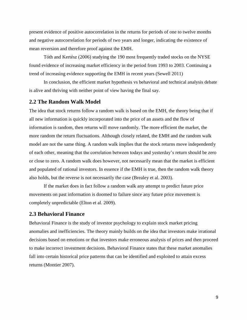
The difference between the opening and closing price is called the candlestick body, it is black if

the closing price is below the opening price and white if the reverse is true (see Figure 1). If the

opening and closing price are identical a Doji is formed meaning the candlestick does not have a

body. The candlesticks can also have upper and/or lower shadows (see Figure 1) which show the

high and low prices achieved respectively during the trading day (Morris 2006).

An extension of candlestick charting is as a technical analysis tool, wherein formations of certain

candlesticks are used to predict future price movement. There are many different distinctive

candlesticks or combination of candlesticks that offer various levels of predictive power. All the

patterns are based on the psychology of the market and a pattern usually consist of one to three

candlesticks but seldom more than five. Some patterns stand on their own, while others need

confirmation to be reliable. Confirmation is often given in the form of a higher opening- or

closing price compared to the previous day in which the candlestick pattern was identified

(Morris 2006).

The candlestick patterns can be sorted into two categories, continuation or reversal patterns.

Continuation patterns indicate that the current trend will continue, while reversal patterns

indicate that the current trend will reverse. Reversal patterns are either bullish or bearish, with

the bearish patterns typically being inverses of the bullish patterns or vice versa (Morris 2006).

Figure 1: Candlestick Construction: Depicts the different parts that make up a candlestick on any given

trading day. Source: Goo, Chen and Chang (2007)

12

2.6 Candlestick Patterns

The Hammer and the Hanging Man: Both are single candlestick trend reversals patterns which

occur in a downwards- and upwards trend respectively. According to Nison (1991) the patterns

have small real bodies with long lower shadows at least 2 times the body’s size and a non-

existent or very small upper shadow (see Figure 2). Morris (2006) explains that the color of the

candlestick becomes more bullish if it is white in a downwards trend and

more bearish if it is black in an upwards trend, but both colors are considered

valid, he goes on to say that the upper shadow should be no more than 10

percent of the high-low range. Nison (1991) recommends waiting for

confirmation of the pattern before committing to any action.

Figure 2: The Hammer or Hanging

Man, depending on trend, both black

and white bodies are valid for each pattern.

The psychology of the Hammer: The market opens in a bearish trend and actors start selling,

however the momentum shifts, the bears begin to lose control resulting in a rally with the price

closing around the opening price. Market participants will observe that the bearish trend has

abated and will therefore be hesitant to enter into a bearish position, bullish actors will be

encouraged to enter long positions, thus prompting a future trend reversal (Morris 2006).

The psychology of the Hanging Man: The market opens in an upwards trend and the price falls

dramatically during the day, the price then rallies to close around the opening price. Market

participants observe that the bullish trend may have begun to slacken off and are therefore

hesitant to maintain their long position the next day, prompting a future trend reversal (Morris

2006).

The Engulfing pattern: Is a major two-day reversal pattern comprised of two real bodies of

opposite color. The second candle’s body completely engulfs the previous day’s candle’s body

(see Figure 3 and 4). The shadows are not part of the pattern. For the pattern to be a viable

indicator the market needs to be in a clear upwards or downwards trend depending on if it is a

bullish or bearish pattern (Nison 1991).

13

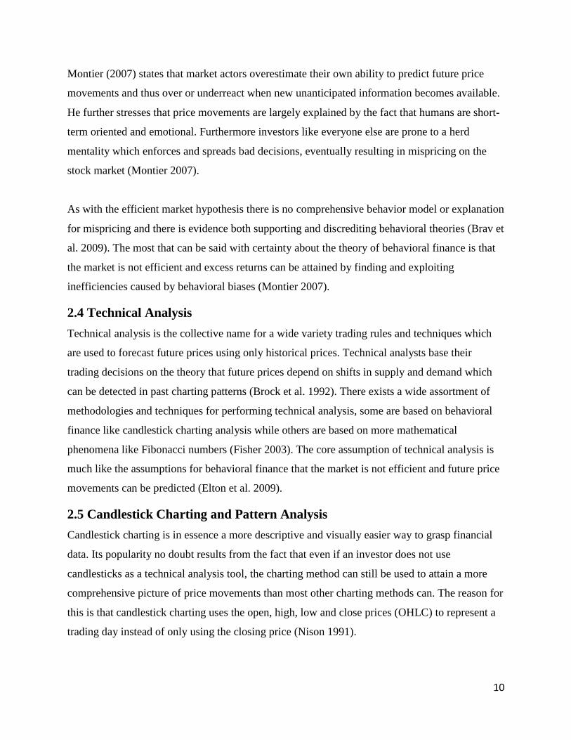
The psychology of the Bullish Engulfing pattern: The Market is in a

downwards trend when a white body open below the previous day’s closing

price and rallies to completely engulf the preceding days black body (see

Figure 3), the change is drastic and the downtrend appears to have stopped

with the bulls gaining control of the market (Nison 1991).

Figure 3: The Bullish

Engulfing Pattern.

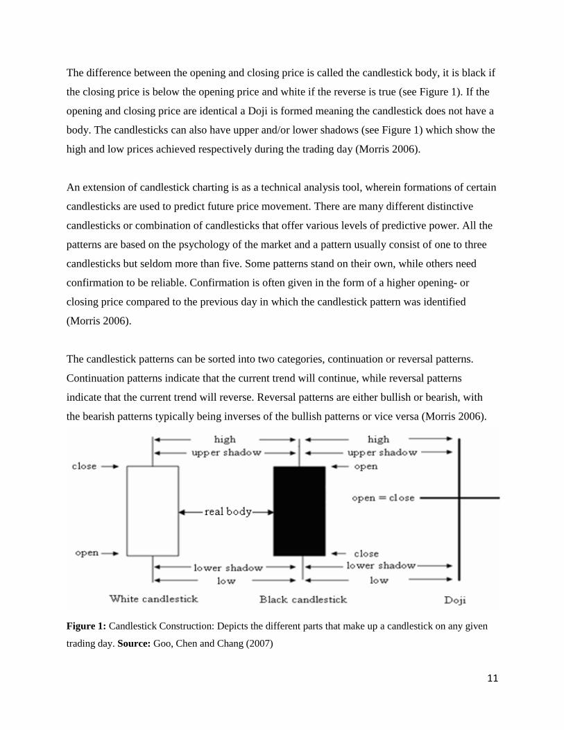
The psychology of the Bearish Engulfing pattern: In an upward trend a

small white body is followed by an open at a new high on the second day,

the new high cannot be maintained and a sell-off calumniates in a close

lower than the previous day’s body (see Figure 4). The momentum of the

upward trend has abated, the bulls are discouraged from staying long and a

major trend reversal towards a downtrend is possible (Nison 1991).

Figure 4: The Bearish

Engulfing Pattern.

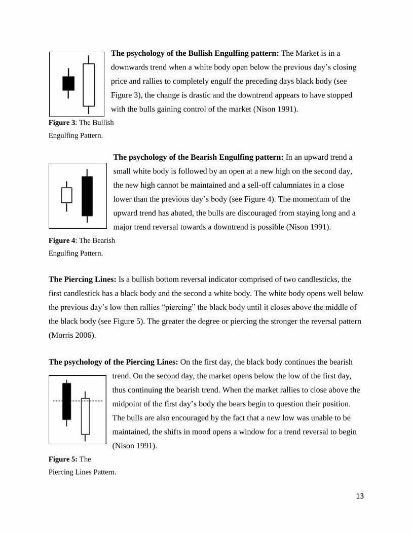
The Piercing Lines: Is a bullish bottom reversal indicator comprised of two candlesticks, the

first candlestick has a black body and the second a white body. The white body opens well below

the previous day’s low then rallies “piercing” the black body until it closes above the middle of

the black body (see Figure 5). The greater the degree or piercing the stronger the reversal pattern

(Morris 2006).

The psychology of the Piercing Lines: On the first day, the black body continues the bearish

trend. On the second day, the market opens below the low of the first day,

thus continuing the bearish trend. When the market rallies to close above the

midpoint of the first day’s body the bears begin to question their position.

The bulls are also encouraged by the fact that a new low was unable to be

maintained, the shifts in mood opens a window for a trend reversal to begin

(Nison 1991).

Figure 5: The

Piercing Lines Pattern.

14

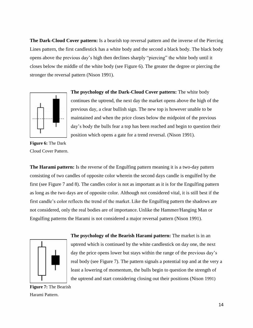
The Dark-Cloud Cover pattern: Is a bearish top reversal pattern and the inverse of the Piercing

Lines pattern, the first candlestick has a white body and the second a black body. The black body

opens above the previous day’s high then declines sharply “piercing” the white body until it

closes below the middle of the white body (see Figure 6). The greater the degree or piercing the

stronger the reversal pattern (Nison 1991).

The psychology of the Dark-Cloud Cover pattern: The white body

continues the uptrend, the next day the market opens above the high of the

previous day, a clear bullish sign. The new top is however unable to be

maintained and when the price closes below the midpoint of the previous

day’s body the bulls fear a top has been reached and begin to question their

position which opens a gate for a trend reversal. (Nison 1991).

Figure 6: The Dark

Cloud Cover Pattern.

The Harami pattern: Is the reverse of the Engulfing pattern meaning it is a two-day pattern

consisting of two candles of opposite color wherein the second days candle is engulfed by the

first (see Figure 7 and 8). The candles color is not as important as it is for the Engulfing pattern

as long as the two days are of opposite color. Although not considered vital, it is still best if the

first candle’s color reflects the trend of the market. Like the Engulfing pattern the shadows are

not considered, only the real bodies are of importance. Unlike the Hammer/Hanging Man or

Engulfing patterns the Harami is not considered a major reversal pattern (Nison 1991).

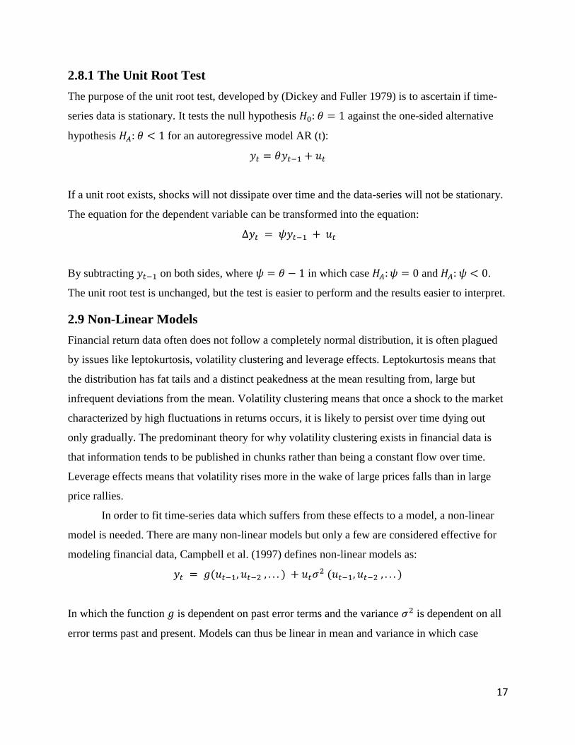
The psychology of the Bearish Harami pattern: The market is in an

uptrend which is continued by the white candlestick on day one, the next

day the price opens lower but stays within the range of the previous day’s

real body (see Figure 7). The pattern signals a potential top and at the very a

least a lowering of momentum, the bulls begin to question the strength of

the uptrend and start considering closing out their positions (Nison 1991)

Figure 7: The Bearish

Harami Pattern.

15

The psychology of the Bullish Harami pattern: In a downtrend a long black day occurs

confirming the trend, on the following day the price opens higher than the close of the previous

day (see figure 8). The higher open creates doubt among the investors who are short, they cover

their positions resulting in a price rally. The rally is however stifled by

speculative short position traders who have yet to enter the market, they see

the increase in price as an opportunity to cash in on the inevitable

continuation of the downtrend. Confirmation on the third day results in the

short positions quickly being covered leading to a further rally, a trend

reversal has begun (Nison 1991).

Figure 8: The Bullish

Harami Pattern.

2.7 The Simple Moving Average

The Simple moving average (MA) is a trend smoothing tool which calculates the mean of the

prices for an asset over a set period of days. The MA eliminates temporary and extreme

fluctuations in price and simplifies the identification of a trend. The more days and therefore

prices that are included in the MA the less emphasis is placed on each individual price. Hence,

more days results in a smoother trend and less risk for single extreme price shifts to influence the

trend. Including more days in the MA results in fewer incorrect trend reversal signals, the cost

however, is a slower recognition of actual trend reversals (Investopedia 2016).

2.8 Stationarity1

A stationary data series is defined as having a constant mean, variance and autocorrelation for

any given lag. In a stationary process a shock dies out over time, diminishing with every

observation from its occurrence, in essence, a shock at time t will have a smaller effect on (t+1)

and even smaller (t+2) etc. For non-stationary data this is not the case, rather than dying out, the

effect of a shock can continue forever. There are two types of non-stationary models, the trend-

1 Note that the entire text involving stationarity and non-linear model uses Chris Brooks, Introductory

Econometrics for Finance 2014 as a source unless otherwise stated – This notation is meant to avoid

excessive referencing to the same source throughout this section of the paper.

16

stationary process model, which is stationary around a linear trend and the random walk model,

of which we are only interested in the latter.

The efficient market hypothesis and the rational expectation hypothesis states that asset

prices should follow a random walk with drift, such a model is given by the equation:

𝑦𝑡 = 𝜇 + 𝑦𝑡−1 + 𝑢𝑡

Where 𝑦𝑡 denotes the dependent variable, 𝜇 denotes the mean, 𝑦𝑡−1 is the dependent variable

lagged once, and 𝑢𝑡 is the error term.

The random walk model can in turn be modified by adding the 𝜃 term:

𝑦𝑡 = 𝜇 + 𝜃𝑦𝑡−1 + 𝑢𝑡

In which case the model falls into three categories depending on the value the 𝜃 term.

The first category is given by:

|𝜃| < 1 ⇒ 𝜃𝑡 → 0 𝑎𝑠 𝑡 → ∞

In which case the model is stationary since the shocks will gradually dissipate over time.

The second category is given by:

𝜃 = 1 ⇒ 𝜃𝑡= 1 ∀ 𝑡

In which case:

𝑦𝑡 = 𝑦0 + ∑ 𝑢𝑡

∞

𝑡=0

𝑎𝑠 𝑡 → ∞

Where the current value of the dependent variable 𝑦𝑡 is simply an infinite sum of the past shocks

and whatever starting point 𝑦0 exists. When 𝜃 = 1 a process is said to have a unit root, and is

non-stationary since the shocks never die out.

The third category in which 𝜃 > 1 describes a process in which any shocks builds upon

another and neither will ever die out. This category will not be considered further since it has few

real world applications.

17

2.8.1 The Unit Root Test

The purpose of the unit root test, developed by (Dickey and Fuller 1979) is to ascertain if time-

series data is stationary. It tests the null hypothesis 𝐻0: 𝜃 = 1 against the one-sided alternative

hypothesis 𝐻𝐴: 𝜃 < 1 for an autoregressive model AR (t):

𝑦𝑡 = 𝜃𝑦𝑡−1 + 𝑢𝑡

If a unit root exists, shocks will not dissipate over time and the data-series will not be stationary.

The equation for the dependent variable can be transformed into the equation:

∆𝑦𝑡 = 𝜓𝑦𝑡−1 + 𝑢𝑡

By subtracting 𝑦𝑡−1 on both sides, where 𝜓 = 𝜃 − 1 in which case 𝐻𝐴: 𝜓 = 0 and 𝐻𝐴: 𝜓 < 0.

The unit root test is unchanged, but the test is easier to perform and the results easier to interpret.

2.9 Non-Linear Models

Financial return data often does not follow a completely normal distribution, it is often plagued

by issues like leptokurtosis, volatility clustering and leverage effects. Leptokurtosis means that

the distribution has fat tails and a distinct peakedness at the mean resulting from, large but

infrequent deviations from the mean. Volatility clustering means that once a shock to the market

characterized by high fluctuations in returns occurs, it is likely to persist over time dying out

only gradually. The predominant theory for why volatility clustering exists in financial data is

that information tends to be published in chunks rather than being a constant flow over time.

Leverage effects means that volatility rises more in the wake of large prices falls than in large

price rallies.

In order to fit time-series data which suffers from these effects to a model, a non-linear

model is needed. There are many non-linear models but only a few are considered effective for

modeling financial data, Campbell et al. (1997) defines non-linear models as:

𝑦𝑡 = 𝑔(𝑢𝑡−1, 𝑢𝑡−2 , . . . ) + 𝑢𝑡𝜎2 (𝑢𝑡−1, 𝑢𝑡−2 , . . . )

In which the function 𝑔 is dependent on past error terms and the variance 𝜎2 is dependent on all

error terms past and present. Models can thus be linear in mean and variance in which case

18

ARIMA models are appropriate or linear in mean and non-linear in variance in which case

GARCH models are needed.

2.9.1 Autoregressive Volatility Models

Auto regressive (AR) volatility models are a simple means of estimating the non-constant

volatility of time series data, it uses proxies to obtain the daily volatility. One of the standard

proxies used is the squared daily returns, in which case the squared return of day t becomes the

volatility estimate for day t.

2.9.2 Autoregressive Conditionally Heteroscedastic (ARCH) Models

The ARCH model is a non-linear model, it is useful due to the fact that it accounts for financial

data often producing errors that are heteroscedastic and a variance that clusters. In order to model

data with these issues the ARCH model uses a conditional variance denoted 𝜎𝑡2, which depends

on the previous value of the error term squared 𝑢𝑡−12 :

𝜎𝑡2 = 𝛼0 + 𝛼1𝑢𝑡−1

2

The model is an ARCH (1) model due the fact that the conditional variance only depends on one

lagged squared error. The conditional mean which describes how the dependent variable 𝑦𝑡

varies over time and 𝑢𝑡 which is a normally distributed error term is modeled with a simple

regression equation:

𝑦𝑡 = 𝛽0 + ∑ 𝛽𝑖𝑥𝑖

𝑖

𝑖=1

+ 𝑢𝑡

𝑢𝑡~𝑁(0, 𝜎2)

2.9.3 Generalized ARCH (GARCH) Models

The GARCH model is an extension of the ARCH model, it has the same possible equations for

the conditional mean as the ARCH. The models differs in that the GARCH allows the

conditional variance to be dependent not only upon past squared errors but also on its own

previous lags, which means that its conditional variance is given by:

𝜎𝑡2 = 𝛼0 + 𝛼1𝑢𝑡−1

2 + 𝛽𝜎𝑡−12

19

𝜎𝑡2 = 𝑇ℎ𝑒 𝐶𝑜𝑛𝑑𝑖𝑡𝑖𝑜𝑛𝑎𝑙 𝑉𝑎𝑟𝑖𝑎𝑛𝑐𝑒

𝑢𝑡−12 = 𝑇ℎ𝑒 𝑠𝑞𝑢𝑎𝑟𝑒𝑑 𝐸𝑟𝑟𝑜𝑟 𝑇𝑒𝑟𝑚 𝑙𝑎𝑔𝑔𝑒𝑑 𝑜𝑛𝑐𝑒

𝜎𝑡−12 = 𝑇ℎ𝑒 𝐶𝑜𝑛𝑑𝑡𝑖𝑛𝑎𝑙 𝑉𝑎𝑟𝑖𝑎𝑛𝑐𝑒 𝑙𝑎𝑔𝑔𝑒𝑑 𝑜𝑛𝑐𝑒

The model is known as the GARCH (1.1) model, so called, since it has one lag of squared errors

terms and one lag of conditional variance. The reason the GARCH is used instead of the ARCH

model is that it is more efficient and avoids overfitting. This is due to it using only three

parameters to account for an infinite number of squared errors to influence the current

conditional variance, while the ARCH model would have to include every past squared error

term in the equation.

2.9.4 The GARCH-In-Mean Model

Investors are generally assumed to demand higher returns when faced with greater risk, one

problem with the GARCH (1.1) model in this respect is that it does not allow for any interaction

between the conditional mean and the conditional variance. To remedy this issue, Engle, Lilien

and Robins (1987) developed the GARCH-In-Mean model, in which the conditional variance

directly affects the conditional mean. The model allows the conditional mean to vary over time

as the degree of risk varies. The model is given by:

𝑦𝑡 = 𝛼 + 𝛾𝜎𝑡2 + 𝛽1𝑢𝑡−1 + 𝑢𝑡

𝜎𝑡2 = 𝛼0 + 𝛼1𝑢𝑡−1

2 + 𝛽2𝜎𝑡−12

𝑢𝑡~𝑁(0, 𝜎2)

𝑦𝑡 = 𝑇ℎ𝑒 𝐶𝑜𝑛𝑑𝑖𝑡𝑖𝑜𝑛𝑎𝑙 𝑀𝑒𝑎𝑛

𝜎𝑡2 = 𝑇ℎ𝑒 𝐶𝑜𝑛𝑑𝑖𝑡𝑖𝑜𝑛𝑎𝑙 𝑉𝑎𝑟𝑖𝑎𝑛𝑐𝑒

𝜎𝑡−12 = 𝑇ℎ𝑒 𝐶𝑜𝑛𝑑𝑖𝑛𝑡𝑖𝑜𝑛𝑎𝑙 𝑉𝑎𝑟𝑖𝑎𝑛𝑐𝑒 𝑙𝑎𝑔𝑔𝑒𝑑 𝑜𝑛𝑐𝑒

𝑢𝑡−1 = 𝑇ℎ𝑒 𝑒𝑟𝑟𝑜𝑟 𝑡𝑒𝑟𝑚 𝑙𝑎𝑔𝑔𝑒𝑑 𝑜𝑛𝑐𝑒

𝑢𝑡 = 𝑇ℎ𝑒 𝐸𝑟𝑟𝑜𝑟 𝑡𝑒𝑟𝑚

The 𝛾 term can be interpreted as a risk premium, if it is positive and statistically significant, then

the returns are dependent on the conditional variance (risk). The error term 𝑢𝑡 is conditionally

normally distributed and serially uncorrelated. And the conditional variance is a linear function

20

of the square of the last period’s error term and the last period’s variance. The model can

therefore properly account for volatility clustering (Brock et al. 1992).

2.10 Bootstrapping

Bootstrapping is a process of creating new random data based on existing data, while keeping the

properties of the original data. Suppose a sample of data exists for which 𝑦𝑡 = 𝑦1, 𝑦2, … , 𝑦𝑡 and

the goal is to estimate a parameter 𝛿, an estimate can be obtained by studying a series of

bootstrapped data. This is done by taking n samples of size T with replacement from the original

𝑦𝑡-series to create new data and then estimating the parameter 𝛿 for each new series of

bootstrapped data. A series of estimated 𝛿 values are thus obtained and they can be used to

estimate the true value of 𝛿. This procedure in essence involves sampling from the sample,

treating the sample as the population from which it is originally drawn.

Bootstrapping in finance is often applied to detect if data-snooping is present in tests for

technical trading rules. Data mining denotes the process of either creating new trading rules

based on existing data and then testing those same rules for significance on a certain data or

applying a multitude of technical rules on price data and choosing any trading rules that by

chance work on the particular set of data.

The bootstrapping methodology when applied to finance can involves bootstrapping the returns

from time-series price-data, this creates data with on average the same distributional properties

as the original, but eliminates any linear or non-linear autocorrelation.

In order to emulate the same price drift, variance and autocorrelation characteristics in the

bootstrapped data that the original possess a different method than the one given above is called

for. This method is in essence comprised of bootstrapping the residuals rather than the returns.

The procedure involves first modeling the returns using an autoregressive model such as

an AR (p), ARCH or GARCH model, whichever fits the data best. Then obtaining its residuals

and bootstrapping them with replacement onto the models equation of estimated parameters

obtained by the autoregressive model. On average this procedure produces a return series that

has the same autoregressive properties as the original series, meaning it can contain auto

regression in the residuals and variance.

21

3. Methodology

3.1 Candlestick Patterns and their Definitions

Candlestick pattern analysis is not an established theory nor one that is rigorously defined. There

are guidelines and recommendations for each pattern in prominent literature by authors like

Nison (1991) and Morris (2006), it is however largely up to each analyst to decide which

constraints to apply to the definitions of each pattern. There are many options, one is to wait for

confirmation of a candlestick pattern before it’s deemed a real pattern. Confirmation for the

study is defined as the closing price being higher on the day following the candlestick being

identified, than the closing price of the last day of the candlestick pattern. Other options include

only recognizing pattern as real when the volume is sufficiently high or when the price

movement during the day is sufficiently large (Nison 1991). Since there exists such an ambiguity

in regards to what a candlestick pattern is supposed to look like, a full outline of the study’s

constraints for all candlestick patterns tested are provided in Appendix 8.2. Furthermore their

excel formulae are presented in Appendix 8.3. The eight candlesticks patterns tested are listed in

Table 1.

Table 1: Candlestick Pattern

Displays the names of the eight candlestick patterns tested in the

study

Bullish Patterns Bullish Patterns

The Hammer The Hanging Man

The Bullish Engulfing The Bearish Engulfing

The Piercing Lines Dark Cloud Cover

The Bullish Harami The Bearish Harami

3.2 Definition of Trend with Moving Averages

All eight candlestick patterns are trend reversal patterns and as such they will only be valid if

they occur in an actual upwards or downwards trend depending on if they are top (bearish) or

bottom (bullish) reversal patterns (Nison 1991). This essentially means that a top reversal pattern

22

in a downward trend is an irrelevant indicator and will be ignored. The reliance of a previous

trend prompts the need for a rigorous definition of trend, this is done by applying a moving

average methodology.

Lu et al. (2011) use a five-day moving average and find that significant returns can be

attained using candlesticks. Marshall et al. (2006) and Marshall et al. (2008) both use a ten-day

exponential moving average and find no significant returns. Caginalp and Laurent (1998) and Lu

(2012) utilize a three-day moving average, and both find significant returns. In order to define

trend for this study, we use a five-day moving average in line with the methodology employed

by Lu and Shiu (2009) as well as Lu et al. (2011). The choice is motivated by it the middle

ground between the ten-day moving average that Marshall et al. (2006) employs and the three-

day moving average employed by Caginalp and Laurent (1998).

The five-day moving average 𝑀𝐴𝑡5 on any given day 𝑡 = 1,2,3 … 𝑛 is given by:

𝑀𝐴𝑡5 =

1

5[𝑝𝑡−4

𝑐 + 𝑝𝑡−3𝑐 + 𝑝𝑡−2

𝑐 + 𝑝𝑡−1𝑐 + 𝑝𝑡

𝑐] (1)

Where 𝑝𝑡𝑐 denotes the closing price on day 𝑡 = 1,2,3 … 𝑛

To identify upward and downward trends the methodology developed by Caginalp and Laurent

(1998) is employed with the slight variation of a five-day MA instead of three-day MA.

An upward trend is identified when the five-day MA is strictly increasing consecutively

for at least five of the past six days. More rigorously stated: At least four of the following five

inequalities have to hold for an upwards trend to be identified:

𝑀𝐴𝑡−55 < 𝑀𝐴𝑡−4

5 … < 𝑀𝐴𝑡−15 < 𝑀𝐴𝑡

5 (2)

And a downwards trend is similarly defined, the difference being that the MA has to be strictly

decreasing instead rather than increasing. Thus, at least four of the following five inequalities

have to hold for a downwards trend to be identified:

𝑀𝐴𝑡−55 > 𝑀𝐴𝑡−4

5 … > 𝑀𝐴𝑡−15 > 𝑀𝐴𝑡

5 (3)

The definition of trend encompassing 6 days is motivated by the focus of the study being on

short term. The allowance for one inequality deviation is motivated by it resulting in a more

flexible definition of trend.

23

3.2.1 A Break in the Trend

In order to define a trend reversal, the methodology outlined by Caginalp and Laurent (1998) is

adopted. The definition of a successful trend reversal according to their methodology is

illustrated by the following scenario which depicts the process of a successful reversal following

a Hammer pattern:

On day (𝑡) a stock is in a downwards trend as defined by Equation (3) and the next day

(𝑡 + 1) a Hammer pattern is identified, the pattern is confirmed the next day (𝑡 + 2) by the

closing price 𝑝𝑡+2𝑐 being higher than on the previous day 𝑝𝑡+1

𝑐 . The trend is successfully reversed

when the following day’s closing price 𝑝𝑡+3𝑐 is lower than the three-day average of the next 3

consecutive days closing prices according to equation 4:

𝑝𝑡+3𝑐 <

1

3[𝑝𝑡+4

𝑐 + 𝑝𝑡+5𝑐 + 𝑝𝑡+6

𝑐 ] (4)

For a bearish pattern, a successful trend reversal is defined by the closing price on day (𝑡 + 3)

being higher than the average of the 3 following days:

𝑝𝑡+3𝑐 >

1

3[𝑝𝑡+4

𝑐 + 𝑝𝑡+5𝑐 + 𝑝𝑡+6

𝑐 ] (5)

A failure of a bullish pattern is confirmed by the closing price 𝑝𝑡+3𝑐 being higher than the average

of the following three days (see Equation 5).

A failure of a bearish pattern is given by the closing price 𝑝𝑡+3𝑐 being lower than the average of

the following three days (see Equation 4).

Although rare, it is also possible for a pattern to result in continuation, which means that the

trend is simply stalled following the identification of a candlestick pattern. The trend being

stalled is not counted as a failure nor as a success. A continuation is defined as:

𝑝𝑡+3𝑐 =

1

3[𝑝𝑡+4

𝑐 + 𝑝𝑡+5𝑐 + 𝑝𝑡+6

𝑐 ] (6)

3.2.2 A Statistical Test for Predictive Power

In order to test if a candlestick is a statistically significant trend reverser we need to examine if

the occurrence of a candlestick pattern in a downtrend (uptrend) increases the probability of

prices moving higher (lower). This is done using the Caginalp and Laurent (1998) methodology,

24

assuming a binominal distribution approximated to the normal distribution. The statistical tests

are performed using a 5% alpha level for significance, applied to a one-sided t-test.

The first step is to ascertain the overall probability of a trend reversal occurring, here

denoted 𝑝0. This is done by first counting the number of times a downward trend reversal occurs

regardless if a candlestick is present or not, this count is denoted 𝑛𝐷. More specifically 𝑛𝐷 is

given by the number of times a downtrend on any given day (t) is followed on day (𝑡 + 3) by a

successful upward signal as defined by equation 4.

The next step is to calculate the total number of days that are in a downtrend as defined

Equation 3, denoted(𝑛𝐴). The overall probability of a downwards trend being reversed 𝑝0, is

then given by the equation:

𝑝0 = 𝑛𝐷/𝑛𝐴

The probability 𝑝0, can according to the central limit theorem be assumed to be the population

mean if the sample satisfies the constraint 𝑛𝐴𝑝0(1 − 𝑝0) > 5 (Körner and Walgren 2006).

The next step is to repeat the process used to count (𝑛𝐷), but in this case only count the number

of times a candlestick reversal pattern is present prior to the trend reversal, this number is

denoted (𝑛𝐶). Next, the number of times the pattern occurs in a downwards trend is counted,

regardless if it is followed by a successful reversal signal as defined by equation 4 or not, the

number is denoted (𝑛𝐸).

It is now possible to calculate the probability of trend reversal success 𝑝𝐶 for the

candlestick pattern:

𝑝𝐶 = 𝑛𝐶/𝑛𝐸

Körner and Walgren (2006) state that the standard deviation of the mean is then given by the

square root of the variance for a binomially distributed variable according to the equation:

𝜎 = √𝑛𝐶𝑝0(1 − 𝑝0)

Once the probabilities and standard deviations are calculated, the next step is to set up the null

and alternate hypothesis:

𝐻0: 𝑝1 − 𝑝0 = 0

25

𝐻1: 𝑝1 − 𝑝0 ≠ 0

The t-statistic is calculated by comparing the difference between the expected value 𝑛𝐶𝑝0 (the

expected number of times a candlestick would be followed by a successful reversal signal) and

sample value 𝑛𝐶𝑝1 (the actual number of times the candlestick is followed by a successful

signal), measured in the number of standard deviations from the null hypothesis by:

𝑡 =𝑛(𝑝 − 𝑝0)

𝜎

To calculate the t-statistic for the bearish patterns, the process is adapted by changing the

downtrends to uptrends and reversals up to reversals down.

3.3 Profit Calculation and its Statistical Test

The study is concerned with fixed holding periods from one to ten days, profits are calculated

with the following assumptions: Positions are entered into the opening price of the day following

the candlestick patterns appearance or following the confirmation of a candlestick pattern and the

positions are exited at the closing price of the last day of the holding period. The profits or

holding period returns for long and short positions are calculated with the following equations:

𝑅𝑙𝑜𝑛𝑔 =𝑝𝑡+𝑛

𝑐 − 𝑝𝑡+4𝑜

𝑝𝑡+4𝑜

𝑅𝑠ℎ𝑜𝑟𝑡 = −𝑝𝑡+𝑛

𝑐 − 𝑝𝑡+4𝑜

𝑝𝑡+4𝑜

Where 𝑝𝑡+4𝑜 is the opening price of the day following the appearance candlestick pattern and

𝑝𝑡+𝑛𝑐 is the closing price n day later. As an example of a four day holding period: If at the end of

day (t) the five-day moving average closing price has been increasing consecutively over the past

five days, then an uptrend is in effect. The following day (t+1), a Hanging Man pattern is

observed and confirmed on day two (t+2), a short position is then entered into at the opening

price on day (t+3) and closed out at the closing price three days later day (t+6).

26

Following the calculation of the mean rate of return of each candlestick during each of the

holding periods, the average rates of return are t-tested for significance, with the null and

alternate hypothesis:

𝐻0: 𝜇𝑖𝑗 = 0

𝐻1: 𝜇𝑖𝑗 > 0

Where 𝜇𝑖𝑗 represents the mean rate of return for each holding period 𝑖 = 1,2,3 … 10 and

candlestick pattern 𝑗 = 1,2,3 … 8. To test the null hypothesis a simple one sided t-test is used

which is defined by:

𝑡 =�̅�𝑖𝑗 − �̅�0

√𝑆𝑖𝑗 𝑛𝑗⁄

Where �̅�𝑖𝑗 is the sample average holding period return for each holding period 𝑗 = 1,2,3 … 10

and candlestick pattern 𝑖 = 1,2,3 … 8, 𝑛𝑗 corresponds to the number of trades, 𝑆𝑖𝑗 is variance of

the sample, �̅�0 denotes the tested hypothetical mean, and (𝑆𝑖𝑗/𝑛𝑗) is the standard error of the

mean.

3.4 Bootstrapping

Due to financial data often having fatter tails (leptokurtosis) than a normal distribution,

autocorrelation, and conditional heteroscedasticity, a simple t-test is not always applicable

(Brooks 2014). To account for this, a bootstrapping approach which accounts for these problems

is used to generate data by drawing from a sample with replacement.

The first step involves creating daily returns from the individual stock’s closing prices in order to

make the data stationary. Once the returns are obtained a unit root test is applied to make sure the

data is stationary. The unit root null and alternative hypothesis are:

𝐻0: 𝑟 ℎ𝑎𝑠 𝑎 𝑢𝑛𝑖𝑡 𝑟𝑜𝑜𝑡

𝐻1: 𝑟 ℎ𝑎𝑠 𝑎 𝑑𝑜𝑒𝑠 𝑛𝑜𝑡 ℎ𝑎𝑣𝑒 𝑎 𝑢𝑛𝑖𝑡 𝑟𝑜𝑜𝑡

Once the null hypothesis is rejected and the data is considered stationary the next step is to

choose which null-model to fit the data to. Based on the precedence set by Marshall et al. (2006)

and (2008), the closing price data is fitted using the GARCH (1.1), Exponential GARCH

27

(EGARCH), GARCH In-Mean (GARCH-M), and the AR (1) models. The results are very

similar for all models and therefore a single model is chosen. The GARCH-M model is chosen,

this is motivated by it being the most realistic model for financial data, since it allows for the

conditional mean to be influenced by the conditional variance. Another reason for using the

GARCH-M is the fact that it is the model Marshall et al. (2006) and (2008) uses. The GARCH-

M is given by equations 7 through 9, for a more detailed explanation of the model see 2.7.6.

𝑦𝑡 = 𝛼 + 𝛾𝜎𝑡2 + 𝛽1𝑢𝑡−1 + 𝑢𝑡 (7)

𝜎𝑡2 = 𝛼0 + 𝛼1𝑢𝑡−1

2 + 𝛽2𝜎𝑡−12 (8)

𝑢𝑡~𝑁(0, 𝜎2) (9)

Once the parameters for equations 7 and 8 are estimated, the residuals are generated and then

redrawn with replacement to form a new residual series. New variance and return series are then

generated using the estimated parameters for equations 7 and 8 by drawing on the randomly

generated residual series. This procedure creates a return series with the same volatility, drift and

unconditional distribution as the original stock. The constructed returns will however, be

independently and identically distributed (Brock et.al 1992). After constructing the new return

series, the new closing prices need to be calculated:

The closing price for the constructed data series on day 1, denoted 𝑃1𝐵𝑐 , is attained from

the equation:

𝑃1𝐵𝑐 = (1 + 𝑟1) ∗ 𝑃0

𝑐

Where 𝑟1 denotes the constructed return for day 1, and 𝑃0𝑐 is the original closing price for day 0.

The closing price on day 2 for the constructed price series 𝑃2𝐵𝑐 is attained from the

equation:

𝑃2𝐵𝑐 = (1 + 𝑟2) ∗ 𝑃1𝐵

𝑐

Where 𝑟2 is the constructed return for day 2, the process is then repeated to attain each closing

price on day 𝑡 = 3,4,5 … 𝑛 for the entire test period. The entire procedure is repeated 500 times,

each time with a new bootstrapped residual series, resulting in new closing price series, all of

which have the same closing price as the original stock on day 0 and then diverge. The randomly

28

generated closing price-series have on average, the same price drift and conditional variance as

the original stock.

The next step is to attain the opening prices for the new bootstrapped data series. These

are generated, by first calculating the percentage differences between the open and closing prices

for all trading days on the original stock with the equation:

𝐷𝑡 = ln [𝑃𝑡

𝑜

𝑃𝑡𝑐]

Where 𝐷𝑡 denotes the percentage difference, 𝑃𝑡𝑜 the opening price of the original data, and 𝑃𝑡

𝑐 the

closing price of the original data for day 𝑡 = 1,2, . . 𝑛.

The differences are then bootstrapped to attain a new random open price percentage

difference series. These are used to construct the new opening prices series with the following

equation:

𝑃𝑡𝐵𝑂 = 𝑒𝐷𝑡 ∗ 𝑃𝑡𝐵

𝑐

Where 𝑒𝐷𝑡 is the exponiated difference 𝐷𝑡, 𝑃𝑡𝐵𝐶 is the constructed closing price and 𝑃𝑡𝐵

𝑂 is the

constructed opening price, all for any day 𝑡 = 0,1,2 … 𝑛. The method is repeated with slight

variations for the high and low percentage differences to attain the new random high and low

price series.

Once the new OHLC time-series data is constructed, the same candlestick trading and

trend rules which are applied on the original data are applied to the new price series. The average

returns for each candlestick pattern and holding period are then compared to that of the original

stock to see which is larger. This process is repeated for each of the 500 randomly generated

OHLC price-data series. If the random price-series generates lower holding period returns than

the original less than five percent of the time, a candlestick pattern’s average holding return is

determined to be statistically significant. The test is therefore a one sided test with a 5% alpha

level (Marshall et al. 2006)

The choice to bootstrap each stock’s data-series 500 times is motivated by it being

enough to give a good approximation of the return distribution of the original data (Brock et.al

1992).

29

3.5 Reliability and Validity

Reliability is a measure of the trustworthiness and objectivity in the research, it measures to

which degree the same study can be performed with the same method to attain the same results.

Validity states to which degree the study measures that which is it meant to examine, factors

which affect validity include the instruments quality and the research design (Körner &

Wahlgren 2012).

Despite including only stocks that are currently in the OMXS30 index which suffers from

survivor bias, the study is not considered to suffer from the same. This is due to the fact that only

the very short term is examined which places very little reliance on long term trends.

Furthermore the returns from the technical trading strategy are not compared to buy and hold

returns but rather to returns generated from bootstrapped price-series-data which do not suffer

from any bias since they are randomly generated. Therefore survivor bias is not considered to

have any effect on the reliability of validity of the study.

The only factor negatively affecting the reliability is the human error factor, which is

considered to be small but present. The human error factor arises from the fact that mistakes can

occur during the process of manually entering data into Excel and Eviews.

In conclusion, since most research methodology is based on previous peer reviewed

research papers and the results answer the main questions asked, the reliability and validity are

considered to be very high.

30

4. Data

4.1 Data Overview and Collection

The study uses secondary data exclusively, focusing on 29 of the 30 individual stocks

comprising the OMXS30 index. The only stocks included in the index are the 30 most traded

stocks on the Swedish stock market. The tests are performed on the time-series price data of the

29 stocks, which is recorded during the approximate 8 year period from 19 October 2007 to 31

December 2015. The data is attained through NASDAQ OMX Nordic database in the OHLC

format. Since the data is collected from NASDAQ’s official website it is considered of high

quality. Furthermore, the data is already adjusted for dividends, splits and emissions.

4.2 Data Selection

The stocks comprising the OMXS30 are thought to be a good approximation of the Swedish

stock market since they are the most traded stocks and thus not subject to isolated inefficiencies

that might occur in low traded stocks. Furthermore, according to Morris (1995) technical

analysis is more applicable to frequently traded stocks, making the index stocks a good choice.

Although the OMXS30 is adjusted every six months in order to properly reflect the changes in

the Swedish stock market, only the stocks included in the index 20 April 2016 are used. The Alfa

Laval AB stock is excluded from the study due to the fact that open and high price data is not

recorded for the entire eight year period. Consequently only 29 of the most traded stocks in the

Swedish stock market are included in the study.

The time period is chosen for several reasons, the main one being that opening price data

is not recorded for any stock prior to 19 October 2007. The period examined encompasses a

crash, from 2007 to 2009, and a recession, from 2008 to 2015 (see figure 9). Since the period

encompasses an entire bust-recession cycle it is considered to give a good overall picture of the

Swedish economy and therefore the stock market. The picture is however not complete, given

that no “boom” is contained within the data period.

31

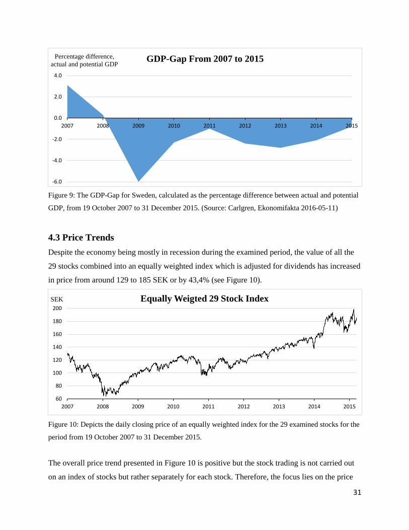
Figure 9: The GDP-Gap for Sweden, calculated as the percentage difference between actual and potential

GDP, from 19 October 2007 to 31 December 2015. (Source: Carlgren, Ekonomifakta 2016-05-11)

4.3 Price Trends

Despite the economy being mostly in recession during the examined period, the value of all the

29 stocks combined into an equally weighted index which is adjusted for dividends has increased

in price from around 129 to 185 SEK or by 43,4% (see Figure 10).

Figure 10: Depicts the daily closing price of an equally weighted index for the 29 examined stocks for the

period from 19 October 2007 to 31 December 2015.

The overall price trend presented in Figure 10 is positive but the stock trading is not carried out

on an index of stocks but rather separately for each stock. Therefore, the focus lies on the price

-6.0

-4.0

-2.0

0.0

2.0

4.0

2007 2008 2009 2010 2011 2012 2013 2014 2015

Percentage difference,

actual and potential GDPGDP-Gap From 2007 to 2015

60

80

100

120

140

160

180

200

2007 2008 2009 2010 2011 2012 2013 2014 2015

SEK Equally Weigted 29 Stock Index

32

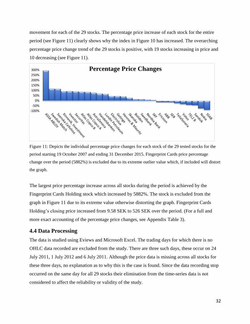
movement for each of the 29 stocks. The percentage price increase of each stock for the entire

period (see Figure 11) clearly shows why the index in Figure 10 has increased. The overarching

percentage price change trend of the 29 stocks is positive, with 19 stocks increasing in price and

10 decreasing (see Figure 11).

Figure 11: Depicts the individual percentage price changes for each stock of the 29 tested stocks for the

period starting 19 October 2007 and ending 31 December 2015. Fingerprint Cards price percentage

change over the period (5882%) is excluded due to its extreme outlier value which, if included will distort

the graph.

The largest price percentage increase across all stocks during the period is achieved by the

Fingerprint Cards Holding stock which increased by 5882%. The stock is excluded from the

graph in Figure 11 due to its extreme value otherwise distorting the graph. Fingerprint Cards

Holding’s closing price increased from 9.58 SEK to 526 SEK over the period. (For a full and

more exact accounting of the percentage price changes, see Appendix Table 3).

4.4 Data Processing

The data is studied using Eviews and Microsoft Excel. The trading days for which there is no

OHLC data recorded are excluded from the study. There are three such days, these occur on 24

July 2011, 1 July 2012 and 6 July 2011. Although the price data is missing across all stocks for

these three days, no explanation as to why this is the case is found. Since the data recording stop

occurred on the same day for all 29 stocks their elimination from the time-series data is not

considered to affect the reliability or validity of the study.

-100%

-50%

0%

50%

100%

150%

200%

250%

300% Percentage Price Changes

33

4.5 Taxes

Taxes are not be considered in this study, this is motivated by that including taxes distracts from

the main focus which is to test if a trading strategy is profitable. Furthermore taxes are not the

same across the world and therefore additional assumptions will have to be made to properly

account for them.

4.6 Courtage

The only relevant transaction costs when trading with stocks is the courtage costs. The current

courtage cost is very low corresponding to 0,085% of the transaction value, which is the

“medium” courtage class cost on the internet based trading hub Avanza (Avanza 2016). Bigger

customers such as firms or banks are however likely to have access to even lower courtage costs.

If courtage is assumed to be 0,085% while another market actor is in fact faced with a lower

courtage, then this incorrect assumption could result in a false negative or type II error. This, of

course, means that the hypothesis of the trading strategy being unprofitable is not rejected

although it should be. With this in mind, courtage costs are not applied to the empirical result.

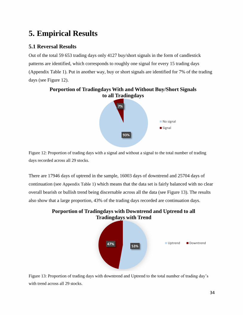
34

5. Empirical Results

5.1 Reversal Results

Out of the total 59 653 trading days only 4127 buy/short signals in the form of candlestick

patterns are identified, which corresponds to roughly one signal for every 15 trading days

(Appendix Table 1). Put in another way, buy or short signals are identified for 7% of the trading

days (see Figure 12).

Figure 12: Proportion of trading days with a signal and without a signal to the total number of trading

days recorded across all 29 stocks.

There are 17946 days of uptrend in the sample, 16003 days of downtrend and 25704 days of

continuation (see Appendix Table 1) which means that the data set is fairly balanced with no clear

overall bearish or bullish trend being discernable across all the data (see Figure 13). The results

also show that a large proportion, 43% of the trading days recorded are continuation days.

Figure 13: Proportion of trading days with downtrend and Uptrend to the total number of trading day’s

with trend across all 29 stocks.

93%

7%

Porportion of Tradingdays With and Without Buy/Short Signals

to all Tradingdays

No signal

Signal

53%47%

Porportion of Tradingdays with Downtrend and Uptrend to all

Tradingdays with Trend

Uptrend Downtrend

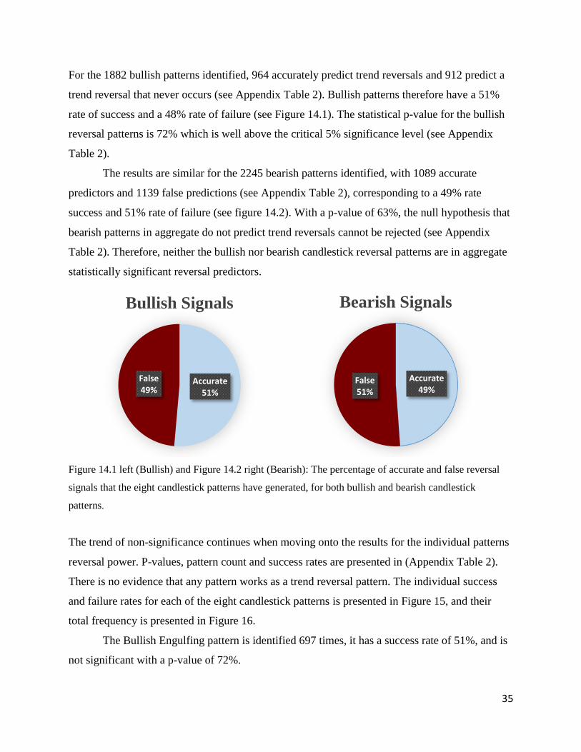
35

For the 1882 bullish patterns identified, 964 accurately predict trend reversals and 912 predict a

trend reversal that never occurs (see Appendix Table 2). Bullish patterns therefore have a 51%

rate of success and a 48% rate of failure (see Figure 14.1). The statistical p-value for the bullish

reversal patterns is 72% which is well above the critical 5% significance level (see Appendix

Table 2).

The results are similar for the 2245 bearish patterns identified, with 1089 accurate

predictors and 1139 false predictions (see Appendix Table 2), corresponding to a 49% rate

success and 51% rate of failure (see figure 14.2). With a p-value of 63%, the null hypothesis that

bearish patterns in aggregate do not predict trend reversals cannot be rejected (see Appendix

Table 2). Therefore, neither the bullish nor bearish candlestick reversal patterns are in aggregate

statistically significant reversal predictors.

Figure 14.1 left (Bullish) and Figure 14.2 right (Bearish): The percentage of accurate and false reversal

signals that the eight candlestick patterns have generated, for both bullish and bearish candlestick

patterns.

The trend of non-significance continues when moving onto the results for the individual patterns

reversal power. P-values, pattern count and success rates are presented in (Appendix Table 2).

There is no evidence that any pattern works as a trend reversal pattern. The individual success

and failure rates for each of the eight candlestick patterns is presented in Figure 15, and their

total frequency is presented in Figure 16.

The Bullish Engulfing pattern is identified 697 times, it has a success rate of 51%, and is

not significant with a p-value of 72%.

Accurate51%

False49%

Bullish Signals

Accurate49%

False51%

Bearish Signals

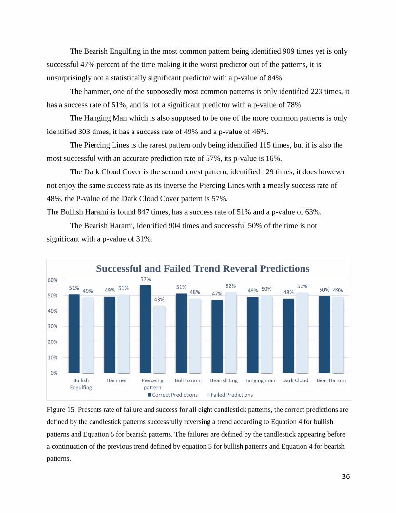
36

The Bearish Engulfing in the most common pattern being identified 909 times yet is only

successful 47% percent of the time making it the worst predictor out of the patterns, it is

unsurprisingly not a statistically significant predictor with a p-value of 84%.

The hammer, one of the supposedly most common patterns is only identified 223 times, it

has a success rate of 51%, and is not a significant predictor with a p-value of 78%.

The Hanging Man which is also supposed to be one of the more common patterns is only

identified 303 times, it has a success rate of 49% and a p-value of 46%.

The Piercing Lines is the rarest pattern only being identified 115 times, but it is also the

most successful with an accurate prediction rate of 57%, its p-value is 16%.

The Dark Cloud Cover is the second rarest pattern, identified 129 times, it does however

not enjoy the same success rate as its inverse the Piercing Lines with a measly success rate of

48%, the P-value of the Dark Cloud Cover pattern is 57%.

The Bullish Harami is found 847 times, has a success rate of 51% and a p-value of 63%.

The Bearish Harami, identified 904 times and successful 50% of the time is not

significant with a p-value of 31%.

Figure 15: Presents rate of failure and success for all eight candlestick patterns, the correct predictions are

defined by the candlestick patterns successfully reversing a trend according to Equation 4 for bullish

patterns and Equation 5 for bearish patterns. The failures are defined by the candlestick appearing before

a continuation of the previous trend defined by equation 5 for bullish patterns and Equation 4 for bearish

patterns.

51% 49%

57%

51%47%

49% 48% 50%49% 51%

43%48%

52%50% 52%

49%

0%

10%

20%

30%

40%

50%

60%

BullishEngulfing

Hammer Pierceingpattern

Bull harami Bearish Eng Hanging man Dark Cloud Bear Harami

Successful and Failed Trend Reveral Predictions

Correct Predictions Failed Predictions

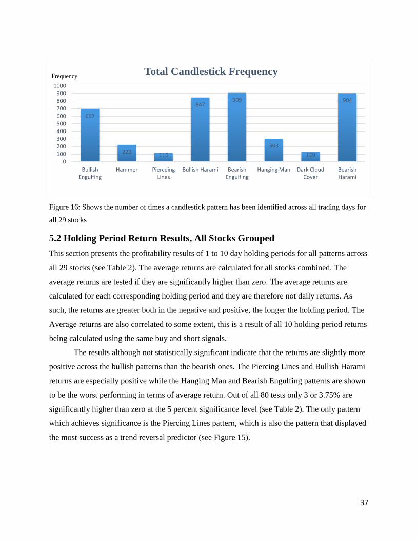
37

Figure 16: Shows the number of times a candlestick pattern has been identified across all trading days for

all 29 stocks

5.2 Holding Period Return Results, All Stocks Grouped

This section presents the profitability results of 1 to 10 day holding periods for all patterns across

all 29 stocks (see Table 2). The average returns are calculated for all stocks combined. The

average returns are tested if they are significantly higher than zero. The average returns are

calculated for each corresponding holding period and they are therefore not daily returns. As

such, the returns are greater both in the negative and positive, the longer the holding period. The

Average returns are also correlated to some extent, this is a result of all 10 holding period returns

being calculated using the same buy and short signals.

The results although not statistically significant indicate that the returns are slightly more

positive across the bullish patterns than the bearish ones. The Piercing Lines and Bullish Harami

returns are especially positive while the Hanging Man and Bearish Engulfing patterns are shown

to be the worst performing in terms of average return. Out of all 80 tests only 3 or 3.75% are

significantly higher than zero at the 5 percent significance level (see Table 2). The only pattern

which achieves significance is the Piercing Lines pattern, which is also the pattern that displayed

the most success as a trend reversal predictor (see Figure 15).

697

223115

847909

303

129

904

0100200300400500600700800900

1000

BullishEngulfing

Hammer PierceingLines

Bullish Harami BearishEngulfing

Hanging Man Dark CloudCover

BearishHarami

FrequencyTotal Candlestick Frequency

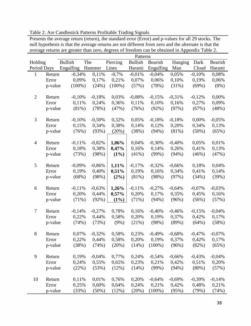
38

Table 2: Are Candlestick Patterns Profitable Trading Signals

Presents the average return (return), the standard error (Error) and p-values for all 29 stocks. The

null hypothesis is that the average returns are not different from zero and the alternate is that the

average returns are greater than zero, degrees of freedom can be obtained in Appendix Table 2.

Patterns

Holding

Period Days

Bullish

Engulfing

The

Hammer

Piercing

Lines

Bullish

Harami

Bearish

Engulfing

Hanging

Man

Dark

Cloud

Bearish

Harami

1 Return -0,34% 0,11% -0,7% -0,01% -0,04% 0,05% -0,10% 0,08%

Error 0,09% 0,17% 0,21% 0,07% 0,06% 0,10% 0,19% 0,06%

p-value (100%) (24%) (100%) (57%) (78%) (31%) (69%) (8%)

2 Return -0,10% -0,18% 0,03% -0,08% -0,15% -0,31% -0,12% 0,00%

Error 0,11% 0,24% 0,36% 0,11% 0,10% 0,16% 0,27% 0,09%

p-value (81%) (78%) (47%) (76%) (92%) (97%) (67%) (48%)

3 Return -0,10% -0,50% 0,32% 0,05% -0,18% -0,18% 0,00% -0,05%

Error 0,15% 0,34% 0,38% 0,14% 0,12% 0,20% 0,34% 0,13%

p-value (76%) (93%) (20%) (38%) (94%) (81%) (50%) (65%)

4 Return -0,11% -0,82% 1,06% 0,04% -0,30% -0,40% 0,05% 0,01%

Error 0,18% 0,38% 0,47% 0,16% 0,14% 0,26% 0,41% 0,13%

p-value (73%) (98%) (1%) (41%) (99%) (94%) (46%) (47%)

5 Return -0,09% -0,86% 1,11% -0,17% -0,32% -0,66% 0,18% 0,04%

Error 0,19% 0,40% 0,51% 0,19% 0,16% 0,34% 0,41% 0,14%

p-value (68%) (98%) (2%) (81%) (98%) (97%) (34%) (39%)

6 Return -0,11% -0,63% 1,26% -0,11% -0,27% -0,64% -0,07% -0,03%

Error 0,20% 0,44% 0,57% 0,20% 0,17% 0,35% 0,45% 0,16%

p-value (71%) (92%) (1%) (71%) (94%) (96%) (56%) (57%)

7 Return -0,14% -0,27% 0,78% 0,16% -0,40% -0,46% -0,15% -0,04%

Error 0,22% 0,44% 0,58% 0,20% 0,19% 0,37% 0,42% 0,17%

p-value (74%) (73%) (9%) (21%) (98%) (89%) (64%) (58%)

8 Return 0,07% -0,32% 0,58% 0,23% -0,49% -0,68% -0,47% -0,07%

Error 0,22% 0,44% 0,58% 0,20% 0,19% 0,37% 0,42% 0,17%

p-value (38%) (74%) (20%) (14%) (100%) (96%) (82%) (65%)

9 Return 0,19% -0,04% 0,77% 0,24% -0,54% -0,66% -0,43% -0,04%

Error 0,24% 0,55% 0,65% 0,23% 0,21% 0,42% 0,51% 0,20%

p-value (22%) (53%) (12%) (14%) (99%) (94%) (80%) (57%)

10 Return 0,11% 0,01% 0,76% 0,20% -0,64% -0,69% -0,39% -0,14%

Error 0,25% 0,60% 0,64% 0,24% 0,21% 0,42% 0,48% 0,21%

p-value (33%) (50%) (12%) (20%) (100%) (95%) (79%) (74%)

39

5.3 Bootstrapped Results, Individual Stocks

This section presents the p-value frequencies attained from comparing the average holding

period trading returns for the individual stocks with those attained from the bootstrapped price-

series-data. The 29 stocks generated average returns from 10 holding periods and 8 candlestick

patterns resulting in 2320 average returns to be compared and therefore 2320 p-values. In total

there are 50 statistically significant average holding period returns (see Table 3) which

corresponds to a 2% rate of significance. All the significant returns are constrained to the

Hammer, Hanging Man, Piercing Lines and Dark Cloud Cover patterns. There appears to be no

difference in significance in terms of how long the holding period is, the significant results are

spread randomly throughout the 1 to 10 day holding period range.

Table 3: Profitability of Candlesticks Pattern Analysis

Count of p-values for the bootstrapped holding period return tests for the 29 stocks. All stocks p-

values are summed for each holding period. Price series data is generated using the GARCH-M

model. The p-values for each holding period are counted as significant when the bootstrapped

holding period return is greater than that of original stock less than five percent of the time.

Candlestick Holding Period Days

1 2 3 4 5 6 7 8 9 10

Bullish Patterns

Engulfing 0 0 0 0 0 0 0 0 0 0

Hammer 3 3 0 1 1 1 1 2 2 3

Piercing

Lines 0 1 2 1 1 1 1 1 1 1

Harami 0 0 0 0 0 0 0 0 0 0

Bearish Patterns

Engulfing 0 0 0 0 0 0 0 0 0 0

Hanging 1 1 1 0 1 2 2 2 3 3

Dark

Cloud 1 2 1 2 1 0 0 0 0 0

Harami 0 0 0 0 0 0 0 0 0 0

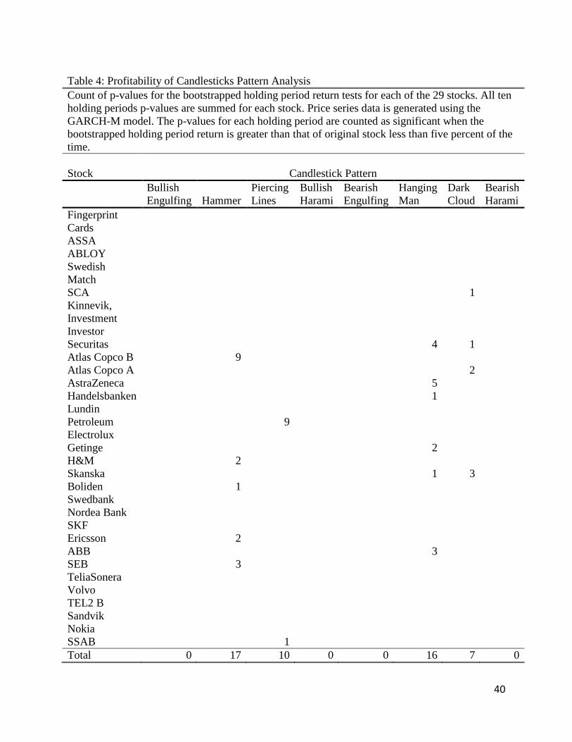
40

Table 4: Profitability of Candlesticks Pattern Analysis

Count of p-values for the bootstrapped holding period return tests for each of the 29 stocks. All ten

holding periods p-values are summed for each stock. Price series data is generated using the

GARCH-M model. The p-values for each holding period are counted as significant when the

bootstrapped holding period return is greater than that of original stock less than five percent of the

time.

Stock Candlestick Pattern

Bullish

Engulfing Hammer

Piercing

Lines

Bullish

Harami

Bearish

Engulfing

Hanging

Man

Dark

Cloud

Bearish

Harami

Fingerprint

Cards

ASSA

ABLOY

Swedish

Match

SCA

1

Kinnevik,

Investment

Investor

Securitas

4 1

Atlas Copco B

9

Atlas Copco A

2

AstraZeneca

5

Handelsbanken

1

Lundin

Petroleum

9

Electrolux

Getinge

2

H&M

2

Skanska

1 3

Boliden

1

Swedbank

Nordea Bank

SKF

Ericsson

2

ABB

3

SEB

3

TeliaSonera

Volvo

TEL2 B

Sandvik

Nokia

SSAB

1

Total 0 17 10 0 0 16 7 0

41

6. Analysis

The objective of the study is to test the predictive power and profitability of eight candlestick

reversal patterns in the short term. To determine these, three statistical tests have been applied to

the empirical results, this chapter analyses the results from these three test.

6.1 Summary Statistics

As mentioned in the result section relatively few trading days with buy or short signals are

identified in relation to the total amount of trading days with roughly one signal being identified

for every 15 days. The relative rarity is likely caused by a number of factors, firstly, only eight

out of many candlestick patterns are studied. Secondly the rigorous definitions of candlestick

patterns utilized is likely to have severely reduced the number of signals. The definitions

incorporate most of the constraints recommended by prominent candlestick literature authors,

including requiring confirmation before a candlestick is verified. Thirdly, the use of a five-day

moving average can be a contributing factor in reducing the number of patterns identified, a

moving average with fewer days will result in a more variable trend which can possibly generate

more signals.

The data has an overall positive price drift trend, with an increase in the 29 stock price index of

43% over the time period. Despite the increase, the proportion of days with uptrend and

downtrend to all days with trend is only slightly skewed towards days with uptrend, with uptrend

days being 6 percentage points more common. An interesting extension of this result is that the

amount of bearish reversal patterns (2245) is larger than the amount of bullish reversal patterns

(1882). Although a bit counterintuitive, this result is logical, for the bearish reversal patterns can

only be found in an uptrend and the bullish patterns only found in a downtrend, and since there is

a slight skew towards uptrend days, a slight skew towards bearish patterns should be evident.

6.2 Predictive Power

Moving on to the predictive power of the candlestick patterns, which is tested using t-test for the

binominal distribution approximated to the normal distribution. The predictive power proves to

be poor across all patterns, with success rates ranging from 48% at the lowest to 58% at the

highest and an average of 51% for bullish patterns and 49% for bearish patterns. These are the

kind of results that are expected in a market where the random walk model holds, any predictive

42

pattern in a random walk would have a success rate of around 50% due to the returns fluctuating

around a mean of zero.

The p-values reflect the poor predictive power, ranging from 16% at the lowest for the

Piercing Lines to 84% at the highest for the Bullish Engulfing pattern, with all the patterns

predictive power being far from the 5% of statistical significance.

The bullish patterns prove to be marginally better predictors than their bearish

counterparts, with 3 out of 4 above the 50% mark in terms of success while the bearish patterns

success rate ranges from 48% to 50%. It is emphasized however, that no pattern except the

Piercing Lines shows any indications of having real predictive power. The marginally better

predictive power attained by the bullish patterns can be a result of random chance.

The results clearly show that predicating trend reversals using the eight candlestick

patterns tested is a futile endeavor. These results lend strong proof for the efficient market

hypothesis and random walk model.

6.3 Profitability Across all Stocks

The average rate of return for all eight candlestick pattern and ten holding periods is with very

few exceptions shown to be lower than is required given the standard error to be statistically

significantly higher than zero. The only pattern shown to be significant is the Piercing Lines

pattern which is statistically greater than zero for 3 out of 10 holding periods. This result has to

be considered cautiously however, considering that the test has a 5% type I error risk and 3 out

of 80 tests or 3.75% are shown be significant. Essentially the significant returns could be a result

of random chance, when a test is performed enough times there will be outliers which lie many

standard deviations from the mean simply due to random happenstance. Because of the fact that

the Piercing Lines pattern is so rare, only being identified 115 times it is especially vulnerable to

type I error. Although it cannot be said that this is the case with absolute certainty, the overall

results do point towards the significance being the result of random chance.

A trading strategy does not have to be statistically significant to be economically viable, the 5%

alpha is in truth, a rather arbitrary choice for significance. Putting statistical analysis aside, the

Piercing Lines pattern shows some promise as a profitable technical analysis trading indicator. It

has an average return of to 1.24% for a 5 day holding period, which when compounded to a

yearly rate of return corresponds to 246%. Although this yearly compounded average return does

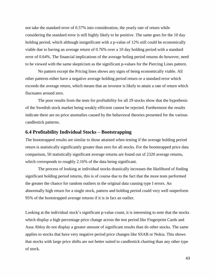
43

not take the standard error of 0.57% into consideration, the yearly rate of return while

considering the standard error is still highly likely to be positive. The same goes for the 10 day

holding period, which although insignificant with a p-value of 12% still could be economically

viable due to having an average return of 0.76% over a 10 day holding period with a standard

error of 0.64%. The financial implications of the average holing period returns do however, need

to be viewed with the same skepticism as the significant p-values for the Piercing Lines pattern.

No pattern except the Pricing lines shows any signs of being economically viable. All

other patterns either have a negative average holding period return or a standard error which

exceeds the average return, which means that an investor is likely to attain a rate of return which

fluctuates around zero.

The poor results from the tests for profitability for all 29 stocks show that the hypothesis

of the Swedish stock market being weakly efficient cannot be rejected. Furthermore the results

indicate there are no price anomalies caused by the behavioral theories presented for the various

candlestick patterns.

6.4 Profitability Individual Stocks – Bootstrapping

The bootstrapped results are similar to those attained when testing if the average holding period

return is statistically significantly greater than zero for all stocks. For the bootstrapped price data

comparison, 50 statistically significant average returns are found out of 2320 average returns,

which corresponds to roughly 2.16% of the data being significant.

The process of looking at individual stocks drastically increases the likelihood of finding

significant holding period returns, this is of course due to the fact that the more tests performed

the greater the chance for random outliers in the original data causing type I errors. An

abnormally high return for a single stock, pattern and holding period could very well outperform

95% of the bootstrapped average returns if it is in fact an outlier.

Looking at the individual stock’s significant p-value count, it is interesting to note that the stocks

which display a high percentage price change across the test period like Fingerprint Cards and

Assa Abloy do not display a greater amount of significant results than do other stocks. The same

applies to stocks that have very negative period price changes like SSAB or Nokia. This shows

that stocks with large price shifts are not better suited to candlestick charting than any other type

of stock.

44

The patterns which generated significant results for the bootstrapping series comparison are all

patterns which are identified the fewest times in the original data. These of course being the

Hammer, Hanging Man, Piecing Lines and Dark Cloud Cover patterns. This is expected,

considering that these patterns are the ones for which outlying data points are given the most

relative weight on the average returns. For the more frequent patterns, the average holding period

return for individual stocks is likely to be a closer approximation of a hypothetical mean, with

less weight given to outlying values.

For example, Lundin Petroleum stands for 9 out of the 10 significant p-values found for

the Piercing Lines pattern. When examining the data further, we find that the pattern is only

identified 4 times for that particular stock and is in this case a 100% successful predictor.

Considering these facts, it seems obvious the stock’s average holding period returns for the

Piercing Lines should outperform those attained with the randomly generated price data series

95% of the time. Furthermore, the holding period return correlation which arises from using the

same trading signals explains why the pattern is significant for 9 out of 10 holding periods.

This example clearly shows that it was a simple result of chance that generated such high

returns for the Piecing Lines pattern when tested on Lundin Petroleum price-data. This is the

weakness of studying individual stock holding period returns for candlestick patterns which are

very rare. Examining Table 4, it is clear that the clustering of significant p-values to certain

stocks and patterns, can be a result of random outliers like the one described for Lundin

Petroleum. The example also illustrates the data-mining properties inherent in using 1 to 10

holding period returns, for eight patterns and 29 stocks. With the calculation of so many p-

values, some are bound to have type I error.

With only 2.16% of the p-values being statistically significantly higher for the original

stocks, the bootstrapping results are more robust than the profitability test for all stocks

combined. As such, the results from bootstrapping lend proof for theory of the Swedish stock

market being weakly efficient.

45

7. Conclusion

The purpose of the study is two-fold, to test if candlestick patterns can predicts future price

movements and to ascertain if they can be used to gain excess returns over the short term. To this

end, three separate statistical test, one for predictive power and two for profitability are carried

out.

The results from the test determining the predicative power using the binomial

distribution t-tests are the least ambiguous. They show that the null hypothesis stating that

candlestick have no predicative power, cannot be rejected. In essence, none of the eight

candlestick patterns appear to have any predicative power when used on Swedish stock data.

The second test is designed to determine if a technical trading strategy based on

candlestick patterns when applied to all 29 stocks in aggregate, can produce holding period

returns which are significantly greater than zero. The results show that the candlestick patterns

have poor profitably when applied to the 29 OMXS stocks. Although some holding period

returns are statistically greater than zero, it is not certain that these are not a result of random

chance.

The third test, like the second is designed to determine if a technical trading strategy

based on the eight candlesticks patterns can produce significant holding period returns. Unlike

the second test however, the bootstrap test compares the holding period returns for each stock

individually. Like the two previous tests, the bootstrapping test indicate that candlestick analysis

holds no value in terms of profitability for investors on the Swedish stock market.

All three tests show that the application of a trading strategy based on candlestick

patterns on the 29 OMXS30 stocks demonstrates neither profitably nor predicative power. The

fact that all three tests show similar results lend proof to the theory of Swedish stock market

being weakly efficient as well as to the random walk model. This study therefore joins a group of

papers that have recently shown that candlesticks perform poorly on well developed markets

such as the S&P500 or the DJIA.

The results also show that bullish patterns are marginally more profitable and display slightly

higher predictive power than bearish patterns. Whether this is a result of the bullish patterns

being better predictors or random chance is difficult to say. The holding periods are shown to be

46

irrelevant in terms of which generate the higher daily returns. Large price-trends which occur

over long periods of time have a no apparent effect on the profitability of candlestick pattern

analysis. This is garnered from the fact that the stocks with the greatest percentage price changes

over the test period performed no better than any other stock did.

Since measuring the success and failure of any pattern is an integral part of the study, it is noted,

that the measuring tool for a pattern’s success or failure as defined by Equation 4 and 5 is shown

to be very powerful. This conclusion is based on the fact that the candlesticks which have a low

rates of success as predictors also have a low average holding period returns. This is illustrated

by the most successful trend reversal predictor, the Piercing Lines having the best and overall

positive profitability results, while the least successful predictor the Bullish Engulfing pattern

has a negative average return for all 10 holding periods.

Although the results fail to reject the hypothesis that the eight candlestick patterns hold no value

for investors, it cannot be stated definitively that candlestick’s as a group are useless to investors.

Different patterns may very well have additional value, the eight candlesticks tested could even

hold value to investors when combined with other technical indicators. Furthermore candlestick

patterns may retain more predictive power when combined with other definitions of trend such as

three-day moving average, exponential average or when trading volume is taken into account.

With the overall results in mind, the author cannot recommend the use of the eight tested

candlestick patterns as technical indicators for short term trading on the Swedish stock market.

Any such attempt is likely to result in negligible profitability or at worst, negative returns.

7.1 Criticism

Candlestick analysis is a broad category of technical analysis, the definitions and use of patterns

is not uniform for all investors. Therefore there are always aspects of candlestick analysis which

are not considered. The study is limited to only eight out of many possible candlestick patterns

and it is therefore difficult to draw any broad conclusions about the profitability of candlestick

pattern analysis in general.

47

The calculations are based on buying and selling at the exact opening and closing prices,

something that in reality is hard to do consistently. This assumption can affect the holding period

returns.

Since the study focuses exclusively on the most traded stocks, it excludes all illiquid equities that

are traded in the Swedish stock market. Although in theory, technical analysis should perform

worse while trading illiquid assets, their exclusion does affect the validity of the study to some

extent.

7.2 Suggestions for Future Studies

Considering the limitations of the study in terms of moving averages, testing different moving

averages and definitions of trend could be very interesting. Previous studies show that the three-

day moving average employed by Lu (2012) as well as Caginalp and Laurent (1998) is the most

successful at finding proof for candlestick pattern profitability. The three-day moving average

does however require more recent research since it has not been tested in developed equity

markets since Caginalp and Laurent (1998) studied the S&P500.

Another interesting aspect of technical analysis to examine is candlestick patterns in conjunction

with other technical indicators such as the RSI or Fibonacci Sequences. Although adding

indicators which are more vulnerable to data mining brings along certain risks such as data

mining, these can mostly be eliminated with the use of a bootstrapping methodology.

Furthermore, this area of candlestick charting has not been explored in any significant way and

could therefore very well find hidden market inefficiencies.

Over the course of this study, it has become clear that the three-day and four-day patterns are

purported to be better than two-day and single day patterns (Farley 2015). It would be interesting

to see if this assumption is true.

The only pattern examined in the study which shows any promise is the Piercing Lines

patterns. Since there is some ambiguity in the results regarding it’s effectiveness, further research

could be warranted.

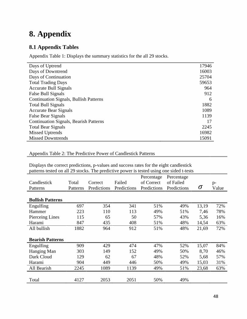
48

8. Appendix

8.1 Appendix Tables

Appendix Table 1: Displays the summary statistics for the all 29 stocks.

Days of Uptrend 17946

Days of Downtrend 16003

Days of Continuation 25704

Total Trading Days 59653

Accurate Bull Signals 964

False Bull Signals 912

Continuation Signals, Bullish Patterns 6

Total Bull Signals 1882

Accurate Bear Signals 1089

False Bear Signals 1139

Continuation Signals, Bearish Patterns 17

Total Bear Signals 2245

Missed Uptrends 16982

Missed Downtrends 15091

Appendix Table 2: The Predictive Power of Candlestick Patterns

Displays the correct predictions, p-values and success rates for the eight candlestick

patterns tested on all 29 stocks. The predictive power is tested using one sided t-tests

Candlestick

Patterns

Total

Patterns

Correct

Predictions

Failed

Predictions

Percentage

of Correct

Predictions

Percentage

of Failed

Predictions 𝜎 p-

Value

Bullish Patterns

Engulfing 697 354 341 51% 49% 13,19 72%

Hammer 223 110 113 49% 51% 7,46 78%

Pierceing Lines 115 65 50 57% 43% 5,36 16%

Harami 847 435 408 51% 48% 14,54 63%

All bullish 1882 964 912 51% 48% 21,69 72%

Bearish Patterns

Engulfing 909 429 474 47% 52% 15,07 84%

Hanging Man 303 149 152 49% 50% 8,70 46%

Dark Cloud 129 62 67 48% 52% 5,68 57%

Harami 904 449 446 50% 49% 15,03 31%

All Bearish 2245 1089 1139 49% 51% 23,68 63%

Total 4127 2053 2051 50% 49%

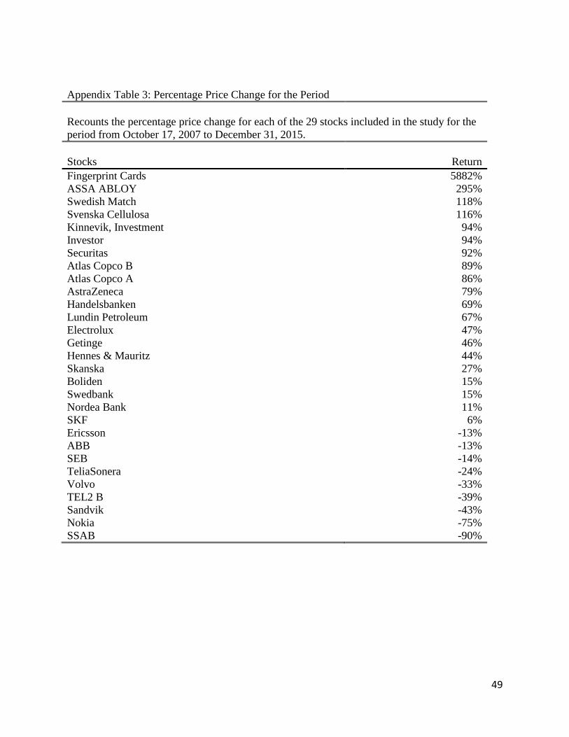
49

Appendix Table 3: Percentage Price Change for the Period

Recounts the percentage price change for each of the 29 stocks included in the study for the

period from October 17, 2007 to December 31, 2015.

Stocks Return

Fingerprint Cards 5882%

ASSA ABLOY 295%

Swedish Match 118%

Svenska Cellulosa 116%

Kinnevik, Investment 94%

Investor 94%

Securitas 92%

Atlas Copco B 89%

Atlas Copco A 86%

AstraZeneca 79%

Handelsbanken 69%

Lundin Petroleum 67%

Electrolux 47%

Getinge 46%

Hennes & Mauritz 44%

Skanska 27%

Boliden 15%

Swedbank 15%

Nordea Bank 11%

SKF 6%

Ericsson -13%

ABB -13%

SEB -14%

TeliaSonera -24%

Volvo -33%

TEL2 B -39%

Sandvik -43%

Nokia -75%

SSAB -90%

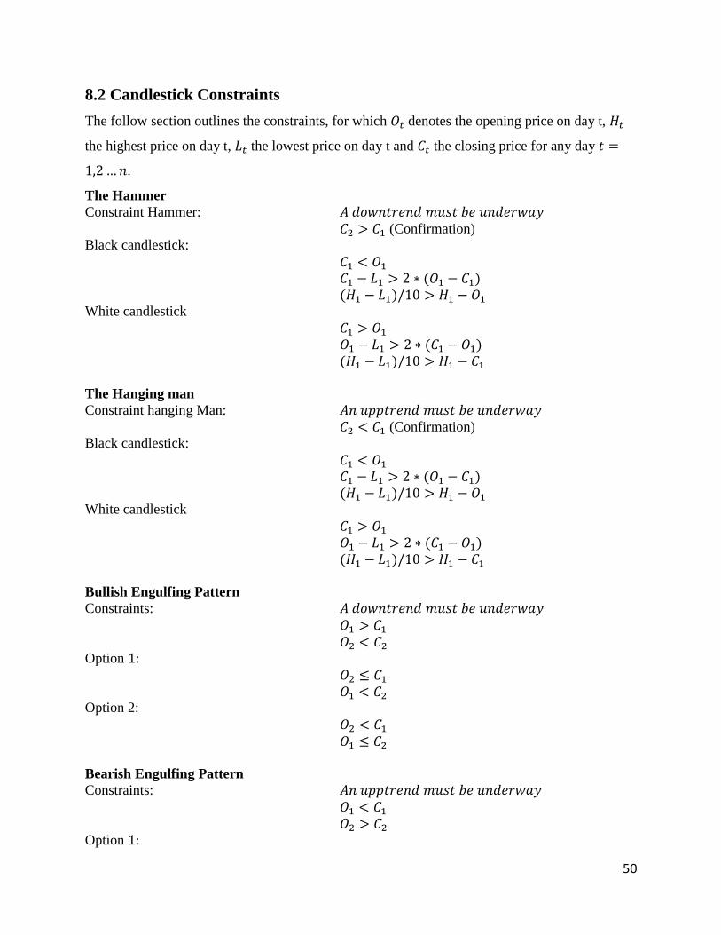
50

8.2 Candlestick Constraints

The follow section outlines the constraints, for which 𝑂𝑡 denotes the opening price on day t, 𝐻𝑡

the highest price on day t, 𝐿𝑡 the lowest price on day t and 𝐶𝑡 the closing price for any day 𝑡 =

1,2 … 𝑛.

The Hammer

Constraint Hammer: 𝐴 𝑑𝑜𝑤𝑛𝑡𝑟𝑒𝑛𝑑 𝑚𝑢𝑠𝑡 𝑏𝑒 𝑢𝑛𝑑𝑒𝑟𝑤𝑎𝑦

𝐶2 > 𝐶1 (Confirmation)

Black candlestick:

𝐶1 < 𝑂1

𝐶1 − 𝐿1 > 2 ∗ (𝑂1 − 𝐶1)

(𝐻1 − 𝐿1)/10 > 𝐻1 − 𝑂1

White candlestick

𝐶1 > 𝑂1

𝑂1 − 𝐿1 > 2 ∗ (𝐶1 − 𝑂1)

(𝐻1 − 𝐿1)/10 > 𝐻1 − 𝐶1

The Hanging man

Constraint hanging Man: 𝐴𝑛 𝑢𝑝𝑝𝑡𝑟𝑒𝑛𝑑 𝑚𝑢𝑠𝑡 𝑏𝑒 𝑢𝑛𝑑𝑒𝑟𝑤𝑎𝑦

𝐶2 < 𝐶1 (Confirmation)

Black candlestick:

𝐶1 < 𝑂1

𝐶1 − 𝐿1 > 2 ∗ (𝑂1 − 𝐶1)

(𝐻1 − 𝐿1)/10 > 𝐻1 − 𝑂1 White candlestick

𝐶1 > 𝑂1

𝑂1 − 𝐿1 > 2 ∗ (𝐶1 − 𝑂1)

(𝐻1 − 𝐿1)/10 > 𝐻1 − 𝐶1

Bullish Engulfing Pattern

Constraints: 𝐴 𝑑𝑜𝑤𝑛𝑡𝑟𝑒𝑛𝑑 𝑚𝑢𝑠𝑡 𝑏𝑒 𝑢𝑛𝑑𝑒𝑟𝑤𝑎𝑦

𝑂1 > 𝐶1

𝑂2 < 𝐶2

Option 1: 𝑂2 ≤ 𝐶1

𝑂1 < 𝐶2 Option 2:

𝑂2 < 𝐶1

𝑂1 ≤ 𝐶2

Bearish Engulfing Pattern

Constraints: 𝐴𝑛 𝑢𝑝𝑝𝑡𝑟𝑒𝑛𝑑 𝑚𝑢𝑠𝑡 𝑏𝑒 𝑢𝑛𝑑𝑒𝑟𝑤𝑎𝑦

𝑂1 < 𝐶1

𝑂2 > 𝐶2

Option 1:

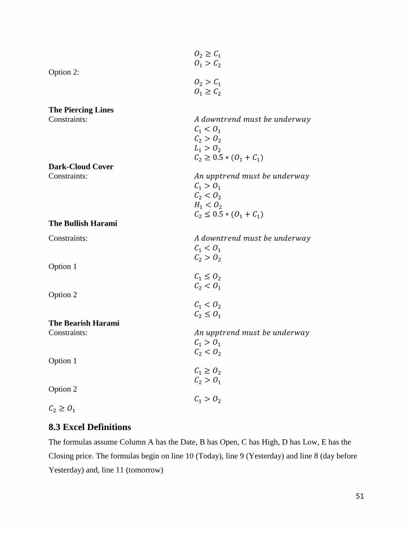
51

𝑂2 ≥ 𝐶1

𝑂1 > 𝐶2 Option 2:

𝑂2 > 𝐶1

𝑂1 ≥ 𝐶2

The Piercing Lines

Constraints: 𝐴 𝑑𝑜𝑤𝑛𝑡𝑟𝑒𝑛𝑑 𝑚𝑢𝑠𝑡 𝑏𝑒 𝑢𝑛𝑑𝑒𝑟𝑤𝑎𝑦

𝐶1 < 𝑂1

𝐶2 > 𝑂2

𝐿1 > 𝑂2

𝐶2 ≥ 0.5 ∗ (𝑂1 + 𝐶1)

Dark-Cloud Cover

Constraints: 𝐴𝑛 𝑢𝑝𝑝𝑡𝑟𝑒𝑛𝑑 𝑚𝑢𝑠𝑡 𝑏𝑒 𝑢𝑛𝑑𝑒𝑟𝑤𝑎𝑦

𝐶1 > 𝑂1

𝐶2 < 𝑂2

𝐻1 < 𝑂2

𝐶2 ≤ 0.5 ∗ (𝑂1 + 𝐶1)

The Bullish Harami

Constraints: 𝐴 𝑑𝑜𝑤𝑛𝑡𝑟𝑒𝑛𝑑 𝑚𝑢𝑠𝑡 𝑏𝑒 𝑢𝑛𝑑𝑒𝑟𝑤𝑎𝑦

𝐶1 < 𝑂1

𝐶2 > 𝑂2 Option 1

𝐶1 ≤ 𝑂2

𝐶2 < 𝑂1 Option 2

𝐶1 < 𝑂2

𝐶2 ≤ 𝑂1

The Bearish Harami

Constraints: 𝐴𝑛 𝑢𝑝𝑝𝑡𝑟𝑒𝑛𝑑 𝑚𝑢𝑠𝑡 𝑏𝑒 𝑢𝑛𝑑𝑒𝑟𝑤𝑎𝑦

𝐶1 > 𝑂1

𝐶2 < 𝑂2 Option 1

𝐶1 ≥ 𝑂2

𝐶2 > 𝑂1 Option 2

𝐶1 > 𝑂2

𝐶2 ≥ 𝑂1

8.3 Excel Definitions

The formulas assume Column A has the Date, B has Open, C has High, D has Low, E has the

Closing price. The formulas begin on line 10 (Today), line 9 (Yesterday) and line 8 (day before

Yesterday) and, line 11 (tomorrow)

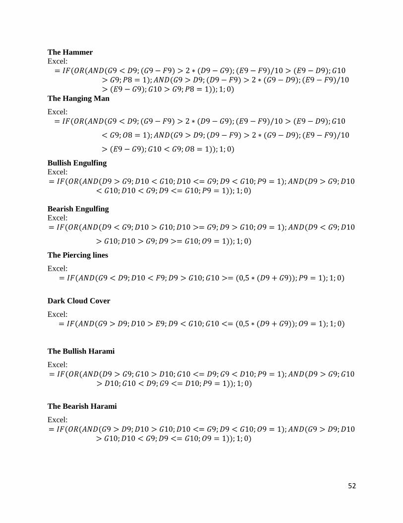
52

The Hammer

Excel:

= 𝐼𝐹(𝑂𝑅(𝐴𝑁𝐷(𝐺9 < 𝐷9; (𝐺9 − 𝐹9) > 2 ∗ (𝐷9 − 𝐺9); (𝐸9 − 𝐹9)/10 > (𝐸9 − 𝐷9); 𝐺10> 𝐺9; 𝑃8 = 1); 𝐴𝑁𝐷(𝐺9 > 𝐷9; (𝐷9 − 𝐹9) > 2 ∗ (𝐺9 − 𝐷9); (𝐸9 − 𝐹9)/10> (𝐸9 − 𝐺9); 𝐺10 > 𝐺9; 𝑃8 = 1)); 1; 0)

The Hanging Man

Excel:

= 𝐼𝐹(𝑂𝑅(𝐴𝑁𝐷(𝐺9 < 𝐷9; (𝐺9 − 𝐹9) > 2 ∗ (𝐷9 − 𝐺9); (𝐸9 − 𝐹9)/10 > (𝐸9 − 𝐷9); 𝐺10

< 𝐺9; 𝑂8 = 1); 𝐴𝑁𝐷(𝐺9 > 𝐷9; (𝐷9 − 𝐹9) > 2 ∗ (𝐺9 − 𝐷9); (𝐸9 − 𝐹9)/10

> (𝐸9 − 𝐺9); 𝐺10 < 𝐺9; 𝑂8 = 1)); 1; 0)

Bullish Engulfing

Excel:

= 𝐼𝐹(𝑂𝑅(𝐴𝑁𝐷(𝐷9 > 𝐺9; 𝐷10 < 𝐺10; 𝐷10 <= 𝐺9; 𝐷9 < 𝐺10; 𝑃9 = 1); 𝐴𝑁𝐷(𝐷9 > 𝐺9; 𝐷10< 𝐺10; 𝐷10 < 𝐺9; 𝐷9 <= 𝐺10; 𝑃9 = 1)); 1; 0)

Bearish Engulfing

Excel:

= 𝐼𝐹(𝑂𝑅(𝐴𝑁𝐷(𝐷9 < 𝐺9; 𝐷10 > 𝐺10; 𝐷10 >= 𝐺9; 𝐷9 > 𝐺10; 𝑂9 = 1); 𝐴𝑁𝐷(𝐷9 < 𝐺9; 𝐷10

> 𝐺10; 𝐷10 > 𝐺9; 𝐷9 >= 𝐺10; 𝑂9 = 1)); 1; 0)

The Piercing lines

Excel:

= 𝐼𝐹(𝐴𝑁𝐷(𝐺9 < 𝐷9; 𝐷10 < 𝐹9; 𝐷9 > 𝐺10; 𝐺10 >= (0,5 ∗ (𝐷9 + 𝐺9)); 𝑃9 = 1); 1; 0)

Dark Cloud Cover

Excel:

= 𝐼𝐹(𝐴𝑁𝐷(𝐺9 > 𝐷9; 𝐷10 > 𝐸9; 𝐷9 < 𝐺10; 𝐺10 <= (0,5 ∗ (𝐷9 + 𝐺9)); 𝑂9 = 1); 1; 0)

The Bullish Harami

Excel:

= 𝐼𝐹(𝑂𝑅(𝐴𝑁𝐷(𝐷9 > 𝐺9; 𝐺10 > 𝐷10; 𝐺10 <= 𝐷9; 𝐺9 < 𝐷10; 𝑃9 = 1); 𝐴𝑁𝐷(𝐷9 > 𝐺9; 𝐺10> 𝐷10; 𝐺10 < 𝐷9; 𝐺9 <= 𝐷10; 𝑃9 = 1)); 1; 0)

The Bearish Harami

Excel:

= 𝐼𝐹(𝑂𝑅(𝐴𝑁𝐷(𝐺9 > 𝐷9; 𝐷10 > 𝐺10; 𝐷10 <= 𝐺9; 𝐷9 < 𝐺10; 𝑂9 = 1); 𝐴𝑁𝐷(𝐺9 > 𝐷9; 𝐷10> 𝐺10; 𝐷10 < 𝐺9; 𝐷9 <= 𝐺10; 𝑂9 = 1)); 1; 0)

53

9. References

Avanza (2016): Prislista för handel i Sverige. Available at: https://www.avanza.se/vart-

utbud/prislista/oversikt/handel-sverige.html (06-05-2016)

Brav Alon, Heaton J. B. and Rosenberg Alexander (2009): The Rational-Behavioral Debate in

Financial Economics - Available at http://people.duke.edu/~alexrose/alonrempaper.pdf - (20-05-

2016)

Brealey Richard and Myers Stewart (2003): Principles of Corporate Companies, Finance

(Seventh Edition - McGraw-Hill Companies, Inc)

Brock William and Lakonishok Josef and LeBaron Blake (1992): Simple Technical

Trading Rules and the Stochastic Properties of Stock Returns (The Journal of Finance, Vol.

47, No. 5, pp. 1731-1764)

Brooks C. 2014: Introductory Econometrics for Finance (3rd Edition, Cambridge University

Press, New York).

Caginalp G. and Laurent H. (1998): The predictive power of price patterns (Applied

Mathematical Finance 5, pp 181–205)

Campbell John, W. Andrew & MacKinlay Craig (1997): The Econometrics of Financial Markets

(Princeton, NJ: Princeton University Press)

Carlgren Fredrik (2016): Högkonjunktur eller lågkonjunktur?: Available at:

http://www.ekonomifakta.se/Fakta/Ekonomi/Tillvaxt/hogkonjunktur-eller-lagkonjunktur/ (17-

05-2016)

Dickey David and Fuller Wayne (1979): Distribution of the Estimators for Autoregressive Time

Series With a Unit Root (Journal of the American Statistical Association Vol. 74, No. 366, pp.

427-431)

Elton, Edwin J. and Gruber, Martin J. and Brown, Stephen J. and Goetzmann, William N.

(2009): Modern Portfolio Theory and Investment Analysis (9th edition, John Wiley & Sons,

Inc.).

Engle Robert, Lilien David, and Robins Russell (1987): Estimating Time Varying Risk Premia in

the Term Structure: The Arch-M Model (Econometrica, Vol. 55, No. 2, 391-407)

Fama E. (1970): Efficient Capital Markets: A Review of Theory and Empirical Work (Journal of

Finance, Vol. 25 (2), pp. 383–417)

Farley Alan (2015): The 5 Most Powerful Candlestick Patterns (NUAN, GMCR) – Available at:

http://www.investopedia.com/articles/active-trading/092315/5-most-powerful-candlestick-

patterns.asp - (25-05-2016)

54

Fischer Robert and Fischer Jens (2003): Candlesticks, Fibonacci, and Chart Pattern Trading

Tools: A Synergistic Strategy to Enhance Profits and Reduce Risk (1st Edition, John Wiley &

Sons Ltd, West Sussex, England)

Frennberg Per and Hansson Björn (1993): Testing the random walk hypothesis on Swedish stock

prices: 1919-l 990 (Journal of Banking and Finance 17 175~191. North-Holland)

Goo, Chen and Chang (2007): The Application of Japanese Candlestick Trading Strategies in

Taiwan (Investment Management and Financial Innovations, Volume 4, Issue 4)

Haugen Robert A. (1995): The New Finance: The Case Against Efficient Markets (1st edition

Englewood Cliffs, N.J: Prentice Hall.)

Hebner Mark (2013): What About the Active Managers Who Have Beaten the Market? -

Available at:

https://www.ifa.com/articles/what_about_active_managers_have_beaten_market_still_need_alph

a_charts/ - (24-05-2016)

Horton, Marshall J. (2009): Stars, crows, and doji: The use of candlesticks in stock selection

(The Quarterly Review of Economics and Finance 49, pp 283–294)

Investopedia (2016): What is a 'Moving Average – MA. Available at:

http://www.investopedia.com/terms/m/movingaverage.asp (21-05-2016)

Jegadeesh N and Titman S. (1993): Returns to Buying Winners and Selling Losers: Implications

for Stock Market Efficiency (The Journal of Finance, Vol. 48, No. 1, pp. 65-91)

Körner S & Wahlgren L (2006): Statistisk Dataanalys (4th edition, Studentlitteratur AB)

Körner S & Wahlgren L (2012): Praktisk Statistik (4th edition, Studentlitteratur AB)

Loomis, Carol J. (2012): Buffett beats the S&P for the 39th year (Fortune Magazine) Available

at: http://fortune.com/2012/02/25/buffett-beats-the-sp-for-the-39th-year/ - (21-05-2016)

Lu Tsung-Hsun (2012): The profitability of candlestick charting in the Taiwan stock market

(Pacific-Basin Finance Journal 26, pp 65–78).

Lu Tsung-Hsun and Shiu, Young-Ming (2009): Tests for Two-Day Candlestick Patterns in the

Emerging Equity Market of Taiwan (Emerging Markets Finance & Trade, Vol. 48, Supplement

1, pp. 41–5)

Lu Tsung-Hsun and Shiu, Young-Ming (2011): Pinpoint and Synergistic Trading Strategies of

Candlesticks (International Journal of Economics and Finance Vol. 3, No. 1, pp 234-244).

55

Marshall, Young and Chang (2008): Are candlestick technical trading strategies profitable in the

Japanese equity market? (Review of Quantitative Finance and Accounting 31, pp 191-207).

Marshall, Young and Rose (2006): Candlestick technical trading strategies: Can they create

value for investors? (Journal of Banking & Finance 30, pp 2303–2323)

Mcgowan Michael (2011): The rise of computerized high frequency trading use and controversy

(Duke Law & Technological Review No. 016)

Montier, James (2007) - Behavioural Investing: A Practitioners Guide to Applying Behavioural

Finance (1st Edition, John Wiley & Sons Ltd, West Sussex, England)

Morris, Gregory L. (1995): Candlestick Charting Explained: Timeless Techniques for Trading

Stocks and Futures (1st Edition The McGraw-Hill Companies, Inc).

Morris, Gregory L. (2006): Candlestick Charting Explained: Timeless Techniques for Trading

Stocks and Futures (3rd Edition The McGraw-Hill Companies, Inc).

Myreteg, Gunilla (2008): Aktiehandel och Internet – Internets påverkan på aktiehandeln och

konsumentbeteende vid aktiehandel på Internet (Örebro universitet Institutionen för ekonomi,

statistik och informatik)

NASDAQ (2006): OMX’s exchanges monthly statistics January 2006 Available at:

http://www.nasdaqbaltic.com/files/riga/statist/2006/OMX_exchanges_statistics_2006_01.pdf -

(16-05-2016)

NASDAQ A (2016): Handelstatistik Februari 2016. Available at:

https://newsclient.omxgroup.com/cdsPublic/viewDisclosure.action?disclosureId=699441&lang=

sv - (11-05-2016)

NASDAQ B (2016): Yearly Nordic Statistics 2000-2015. Available at:

http://www.nasdaqomx.com/digitalAssets/102/102048_yearly_nordic_statistics_2000_2015.xls

(11-05-2016)

Nison Steve (1991): Japanese candlestick charting techniques: A Contemporary Guide to the

Ancient Investment Techniques of the Far East (1st edition, New York Institute of Finance)

Raymond, Yuen Wai Pong (2012): Fundamental Analysis vs Technical Analysis (SSRN

Electronic Journal) – Available at http://papers.ssrn.com/sol3/papers.cfm?abstract_id=2051485

(11-05-2016)

Roberts, Harry (1967): Statistical Versus Clinical Prediction of the Stock Market (Unpublished

manuscript, CRSP, University of Chicago)

SCB: Statistiska Centralbyrån (2006): Hushållen allt rikare. Available at:

http://www.scb.se/sv_/Hitta-statistik/Statistik-efter-

56

amne/Finansmarknad/Aktieagarstatistik/Aktieagarstatistik/6450/6457/Behallare-for-

Press/159583/ - (01-05-2016)

SCB: Statistiska Centralbyrån (2016): Aktieägarstatistik Aktieägande i bolag noterade på svensk

marknadsplats, december 2015. Available at:

http://www.scb.se/Statistik/FM/FM0201/2015H02/FM0201_2015H02_SM_FM20SM1601.pdf -

(01-05-2016)

Sewell, Martin (2011): History of the Efficient Market Hypothesis (UCL department of computer

science) – Available at: http://www.cs.ucl.ac.uk/fileadmin/UCL-

CS/images/Research_Student_Information/RN_11_04.pdf - (11-05-2016)

Tóth and Kertész (2006) Increasing market efficiency: Evolution of cross-correlations of stock

returns (Physica A 360 505–51)