The potential of AltiKa to address SWOT phenomenology (part 1)

SWOT  SDT  mee)ng,  Washington,  January  2014,  14  -­‐  16  

Denis Blumstein, Nathalie Steunou, Nicolas Picot Stéphane Calmant, Fernando Niño

Introduction

AltiKa can bring large scale view of the geophysical situation �  Topography �  Backscatter (not a lot of measurements available in Ka band) But not only. It could also be used to investigate �  Interaction of Ka radar waves with the terrain (surface/volume, absolute calibration) �  Backscatter variability at a few hundred meters scale �  Backscatter angular variation in the range 0, 0.5 degrees of incidence �  … �  With some work (waveforms inversion)

�  Some examples follows

SWOT SDT meeting, Washington, January 2014, 14 - 16 2

Computation of sigma0 in AltiKa products (GDR, SGDR) 1/2

Results of 4 retrackers available (ocean, ice1, ice2, seaice) Main hypothesis �  The surface is flat and horizontal at large scale �  The backscatter is uniform This is consistent with what has been done for Envisat products Other important points �  No correction for atmospheric attenuation applied to σ0 40 Hz �  σ0 ocean must be used with great caution over land �  σ0 ice1 and ice2 do not take into account antenna gain pattern

SWOT SDT meeting, Washington, January 2014, 14 - 16 3

Computation of sigma0 in AltiKa products (GDR, SGDR) 2/2

As is, this provides useful information. But users must be conscious of these hypothesis if they do not work for them. Some examples will be shown �  When the backscattered power comes mainly from a small part of the footprint

(narrow river, coast) �  When there are sharp backscatter contrasts across the scenery �  When there is a terrain slope or « random » variations of altitude

Traditionally, users/scientists for which the preceeding hypothesis do not work (e.g. for glaciology applications) provide their own geophysical corrections

è  Brenner [1983], Rapley [1986], Remy [1989], … è  in these cases, additional information must be used to be able to retrieve the « real »

backscatter of the terrain

SWOT SDT meeting, Washington, January 2014, 14 - 16 4

Waveforms inversion

AltiKa background �  Footprint computed on a flat surface is around 8 km (diameter, 3dB beam limited

footprint, the pulse limited footprint is slightly larger) �  Along track sampling distance is around 160 meters This creates some redundancy in the measurements that can be used to get information at a resolution largely better than the footprint size à waveforms inversion

Inspiration came mainly from 2 papers �  V.Enjolras and E.Rodriguez, Using Altimetry Waveform Data and Ancillary Information

From SRTM, Landsat, and MODIS to Retrieve River Characteristics, 2009 �  J.Tournadre, B.Chapron, N.Reul , High-Resolution Imaging of the Ocean Surface

Backscatter by Inversion of Altimeter Waveforms, 2011 The techniques we use today for the inversion are different And from many fruitful discussions with collegues at LEGOS, CNES and CLS.

SWOT SDT meeting, Washington, January 2014, 14 - 16 5

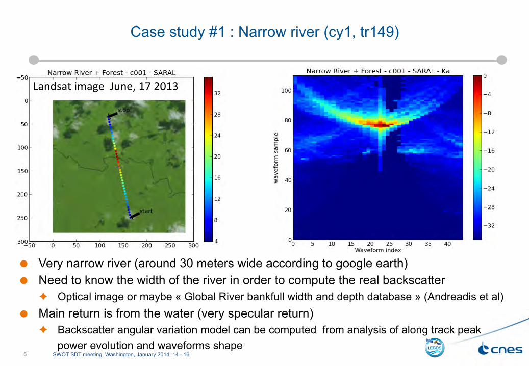
Case study #1 : Narrow river (cy1, tr149)

�  Very narrow river (around 30 meters wide according to google earth) �  Need to know the width of the river in order to compute the real backscatter

è  Optical image or maybe « Global River bankfull width and depth database » (Andreadis et al) �  Main return is from the water (very specular return)

è  Backscatter angular variation model can be computed from analysis of along track peak power evolution and waveforms shape

SWOT SDT meeting, Washington, January 2014, 14 - 16 6

Landsat  image    June,  17  2013  

Case study #2 : Contrast inversion (cy1, tr149)

SWOT SDT meeting, Washington, January 2014, 14 - 16 7

�  Backscatter greater on the island than on the river �  Peak of return power comes from a flat surface (water under the trees ?) �  σ0 = 44 dB (TBC), very specular return

è  backscatter angular variation model = a gaussian with FWHM = 0.05 deg)

Landsat  image    June,  17  2013  

Case study # 3 ─ Hydrology (Japura River) – comparison Ka/Ku

Tr  078   Tr  121  

From a series of 3 crossing points provided by Stéphane Calmant River width 1.8 km

11 SWOT SDT meeting, Washington, January 2014, 14 - 16

Case study #3 ─ Hydrology (Japura River)

Measurements (sigma0 ice1) �  contrast between river and land : inversion between cycle 4 and cycle 5 �  caused by the island ? (closer from satellite track in cycle 5)

SWOT SDT meeting, Washington, January 2014, 14 - 16 9

Landsat  image    December,  29  2013  

Case study #3 – Altitude difference AltiKa - SRTM

Differences versus SRTM � Small on the river � 15 à 20 meters on the forest

Track 78 Cycles 1 to 8 (March to

November)

10  km  

10

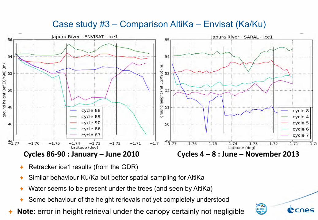
Case study #3 – Comparison AltiKa – Envisat (Ka/Ku)

Cycles  4  –  8  :  June  –  November  2013    Cycles  86-­‐90  :  January  –  June  2010  è  Retracker ice1 results (from the GDR) è  Similar behaviour Ku/Ka but better spatial sampling for AltiKa

è  Water seems to be present under the trees (and seen by AltiKa)

è  Some behaviour of the height rerievals not yet completely understood

è  Note: error in height retrieval under the canopy certainly not negligible

Conclusions and Perspectives

�  This is work in progress �  Waveforms inversion could not be performed on a global scale but for AirSWOT data

analysis or case studies this is possible and can be useful �  Analysis of AltiKa data could also bring our attention on some particular behaviour of

Ka Band phenomenology that must be addressed (for example to develop the SWOT Algorithms)

�  Analyse AltiKa data to get statistically significative distribution of specular returns in Ka over inland water

�  Identify simpler cases for studies of the impact of the incidence angle (0 to 0.5 deg) in case of water under the canopy

è  research : success not guaranted but interest makes worth the effort è  more uniform forests, other areas / kind of forests / wetlands / boreal regions

�  AirSWOT campaigns �  Some activities are planned by CNES project in 2014 regarding backscatter analysis

in Ka band

SWOT SDT meeting, Washington, January 2014, 14 - 16 12

Perspectives (2/2)

In the frame of AltiKa data exploitation �  Comparison of the different retracking methods and the resultant sigma0

estimations �  Comparison of the estimations over some dedicated areas between Ka and Ku �  Studies of high rate AltiKa data : some acquisitions over oceans in high data rate

mode will provide waveforms at the PRF rhythm in amplitude and phase. Analysis of the correlation will be done

Experimental and theoretical studies �  Measurements of backscatter in wind tunnel, with simultaneous measurement in

Ka and Ku band in different wind conditions �  In parallel : improvement of the backscattering models

SWOT SDT meeting, Washington, January 2014, 14 - 16 13

Backup slides

SWOT SDT meeting, Washington, January 2014, 14 - 16 14

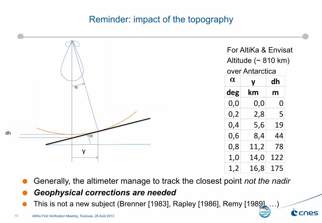
Reminder: impact of the topography

AltiKa First Verification Meeting, Toulouse, 28 Août 2013 15

For AltiKa & Envisat Altitude (~ 810 km) over Antarctica

�  Generally, the altimeter manage to track the closest point not the nadir �  Geophysical corrections are needed �  This is not a new subject (Brenner [1983], Rapley [1986], Remy [1989], …)

α y dhdeg km m0,0 0,0 00,2 2,8 50,4 5,6 190,6 8,4 440,8 11,2 781,0 14,0 1221,2 16,8 175

y  

Impact of terrain slope on the apparent sigma0

SARAL/AltiKa 1st Verification Meeting, Toulouse,, August 2013, 27th-29th 16

0°            0.1°        0.2°            0.3°            0.4°                        0.5°                                      0°            0.1°        0.2°            0.3°            0.4°                        0.5°    

�  Computed with a synthetic antenna diagram (gaussian)

Case study #4 : NorthWest Australia (cy6, tr034)

�  Confirmation that contrast land/sea is around 5 dB Input for the simulation

�  Ocean : σ0 = 11 dB, Land : σ0 = 6 dB (see slide 8 for simulation of the beach) è  But lot of variability of the land surface

SWOT SDT meeting, Washington, January 2014, 14 - 16 17

Case study #4 : NorthWest Australia (cy6, tr034)

Input for the simulation �  Ocean : sigma0 = 11 dB

�  Land : σ0 = 6 dB

SWOT SDT meeting, Washington, January 2014, 14 - 16 18

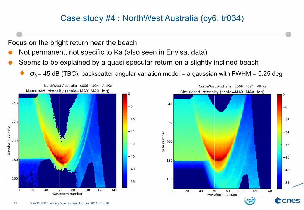
Case study #4 : NorthWest Australia (cy6, tr034)

Focus on the bright return near the beach �  Not permanent, not specific to Ka (also seen in Envisat data) �  Seems to be explained by a quasi specular return on a slightly inclined beach

è  σ0 = 45 dB (TBC), backscatter angular variation model = a gaussian with FWHM = 0.25 deg

SWOT SDT meeting, Washington, January 2014, 14 - 16 19

March-April 2013: measures along the

AltiKa tracks Courtesy  Alexei  Kouraev  

Rough, hummocky (1 cm thick), snow

Smooth, mostly clear ice

Smooth; congelated pancake ice

Snow-covered ice

Double-layered ice

Snow, small patches of clear ice

Snow, small patches of clear ice

Courtesy  Alexei  Kouraev  

466, cycle 1, 30 March 13

Open ice in coastal areas High backscatter when no snow Courtesy  Alexei  Kouraev  

466, cycle 2, 4 May 13

Dramatic decrease of backscatter Courtesy  Alexei  Kouraev  

466, cycle 3, 8 June 13

Open water - but strange high backscatter Courtesy  Alexei  Kouraev