The Potential Effect of Los Angeles Basin Pollution on Grand Canyon Air Quality

by Gregory S. Poulos

Department of Atmospheric Science Colorado State University

Fort Collins, Colorado

Roger A. Pielke, P.1.

The Potential Effect of Los Angeles Basin Pollution on Grand Canyon Air Quality

by Gregory S. Poulos

Department of Atmospheric Science Colorado State University

Fort Collins, Colorado

Roger A. Pielke, P.1.

THE POTENTIAL EFFECT OF LOS ANGELES BASIN POLLUTION ON GRAND

CANYON AIR QUALITY

Gregory S. Poulos

Department of Atmospheric Science

Colorado State University

Fort Collins, Colorado

Spring 1992

Atmospheric Science Paper No. 490

THE POTENTIAL EFFECT OF LOS ANGELES BASIN POLLUTION ON GRAND

CANYON AIR QUALITY

Gregory S. Poulos

Department of Atmospheric Science

Colorado State University

Fort Collins, Colorado

Spring 1992

Atmospheric Science Paper No. 490

The funding for this research was provided by the National Park Service through Interagency Agreement #0475-4-8003 with the National Oceanic and Atmo­spheric Administration through Agreement #CM0200 DOC-NOAA to the Co­operative Institute for Research in the Atmosphere (Project #5-31253).

The funding for this research was provided by the National Park Service through Interagency Agreement #0475-4-8003 with the National Oceanic and Atmo­spheric Administration through Agreement #CM0200 DOC-NOAA to the Co­operative Institute for Research in the Atmosphere (Project #5-31253).

ABSTRACT

THE POTENTIAL EFFECT OF LOS ANGELES BASIN POLLUTION ON GRAND

CANYON AIR QUALITY

This study presents a numerical investigation of air pollutant transport from the Los

Angeles Basin to Grand Canyon National Park (GCNP). The Colorado State University

Regional Atmospheric Modeling System (CSU-RAMS) is used to develop fields of different

atmospheric variables. These fields are applied in a Lagrangian Particle Dispersion Model

(LPDM) to simulate the advection of pollutant particles. It is found that, indeed, under

th,e somewhat idealistic, worst case, initial conditions presented, particles released from

the Los Angeles Basin will impact the Grand Canyon but only in small amounts. By

comparing a flat to complex terrain simulation, the importance of the terrain features

between Los Angeles and GCNP to the dispersion of Los Angeles Basin pollutants is

made obvious. Mountain barriers and undulating land reduce what could otherwise be a

very serious pollutant impact on GCNP. Based on these results the conclusion is made

that under the southwest flow conditions existing during the Winter Haze Intensive Tracer

EXperiment (WHITEX) period of February 10-13, 1987 Los Angeles Basin pollution did

not contribute significantly to visibility reduction in the Grand Canyon. This supports

the WHITEX conclusion that the Navajo Generating Station (NGS) was the primary

contributor during this period of poor haze conditions.

ii

Gregory S. Poulos Department of Atmospheric Science Colorado State University Fort Collins, Colorado 80523 Spring 1992

ABSTRACT

THE POTENTIAL EFFECT OF LOS ANGELES BASIN POLLUTION ON GRAND

CANYON AIR QUALITY

This study presents a numerical investigation of air pollutant transport from the Los

Angeles Basin to Grand Canyon National Park (GCNP). The Colorado State University

Regional Atmospheric Modeling System (CSU-RAMS) is used to develop fields of different

atmospheric variables. These fields are applied in a Lagrangian Particle Dispersion Model

(LPDM) to simulate the advection of pollutant particles. It is found that, indeed, under

th,e somewhat idealistic, worst case, initial conditions presented, particles released from

the Los Angeles Basin will impact the Grand Canyon but only in small amounts. By

comparing a flat to complex terrain simulation, the importance of the terrain features

between Los Angeles and GCNP to the dispersion of Los Angeles Basin pollutants is

made obvious. Mountain barriers and undulating land reduce what could otherwise be a

very serious pollutant impact on GCNP. Based on these results the conclusion is made

that under the southwest flow conditions existing during the Winter Haze Intensive Tracer

EXperiment (WHITEX) period of February 10-13, 1987 Los Angeles Basin pollution did

not contribute significantly to visibility reduction in the Grand Canyon. This supports

the WHITEX conclusion that the Navajo Generating Station (NGS) was the primary

contributor during this period of poor haze conditions.

ii

Gregory S. Poulos Department of Atmospheric Science Colorado State University Fort Collins, Colorado 80523 Spring 1992

ACKNOWLEDGEMENTS

Sincere gratitude is extended to Professor Roger A. Pielke for his thoughtful advising

from beginning to end. In discussions throughout the development of this study, colleagues

and many friends were also important including, Dr. Douglas A. Wesley, Mike Meyers,

Dr. Melville E. Nicholls, Xubin Zeng, Scot Randell, and Mike Moran. In particular, I

would single out Dr. Michael Weissbluth for his advice and role as a confidant. Finally,

no greater thanks and appreciation can be shown than that for my Father and Mother

whose inspiration, guidance, expectations, and love were by far the strongest motivation

for this study. Thank you Dad and Mom. I would also like to extend my thanks to Bryan

Critchfield, Tara Pielke,and Dallas McDonald for the preparation and typing of this thesis.

iii

TABLE OF CONTENTS

1 INTRODUCTION 1

2 BACKGROUND 8 2.1 The WHITEX Report . . . . . . . . . . . . . . . . . . . . . . . . . . . . . . .. 8 2.2 Long-range Transport ... . . . . . . . . . . . . . . . . . . . . . . . . . . . .. 9 2.2.1. Definition...................................... 10 2.2.2 Global........................................ 10 2.2.3 United States. . . . . . . . . . . . . . . . . . • . . . . . . . . . . . . . • . .. 11 2.2.4 Southwest United States. . . . . . . . . . . . . . . . . . . . . . . . . . . . .. 11 2.2.5 Meteorological Effects . . . . . . . . . . . . . . . . . . . . . . . . . . . . . .. 14 2.3 Southern California/Los Angeles Basin Pollution . . . . . . . . . . . . . . . . . 20 2.3.1 Pollutant Sources ................................. 21 2.3.2 Pollutant Flows in the Los Angeles Basin . . . . . . . . . . . . . . . . . . . . 22

3 RAMS MODEL DESCRIPTION 28 3.1 General Description ................................. 28 3.2 RAMS Formulation and Options . . . . . . . . . . . . . . . . . . . . . . . . . . 29 3.2.1 Variables . . . . . . . . . . . . . . . . . . . . . . . . . . . . . . . . . . . . . . 30 3.2.2 Gridding System . . . . . . . . . . . . . . . . . . . . . . . . . . . . . . . . . . 30 3.2.3 Atmospheric Moisture. . . . . . . . . . . . . . . . . . . . . . . . . . . . . . . 31 3.2.4 Radiation...................................... 31 3.2.5 Model Boundaries . . . . . . . . . . . . . . . . . . . . . . . . . . . . . . . .. 32 3.2.6 Model Initialization ................................ 32

35 4 SIMULATIONS AND RESULTS 4.1 RAMS Model Simulations Overview . . . . . . . . . . . . . . . . . . . . . . .. 35 4.2 Lagrangian Particle Dispersion Model Simulations Overview. . . . . . . . . . . 4.3 SW-1: Simulation Analysis ............................ . 4.3.1 Meteorological Results: SW-1 .......................... . 4.3.2 LPDM Results: SWP-1 ............................. . 4.4 SW-2: Simulation Analysis ............................ . 4.4.1 Meteorological Results . . . . . . . . . . . . . . . . . . . . . . . . . . . . . . . 4.4.2 LPDM Results: SWP-2 . . . . . . . . . . . . . . . . . . . . . . . . . . . . . .

37 39 39 56 68 68 93

4.5 SW-3: Simulation Analysis ............................. 104 4.5.1 Meteorological Results: SW-3 . . . . . . . . . . . . . . . . . . . . . . . . . . . 105 4.5.2 LPDM Results: SWP-3 . . . . . . . . . . . . . . . . . . . . . . . . . . . . . . 127

iv

5 SUMMARY AND CONCLUSIONS 135 5.1 Summary . . . . . . . . . . . . . . . . . . . . . . . . . . . . . . . . . . . . . . . 135 5.2 Conclusions...................................... 137

REFERENCES 140

v

LIST OF FIGURES

1.1 Soundings for Page, Arizona during the WHITEX poor haze period in the Grand Canyon, February 10-13, 1987 . . . . . . . . . . . . . . . . . . . . .. 4

1.2 Study region for Los Angeles pollut"ant flow to the Grand Canyon. . . . . . .. 5 1.3 A contoured view of topography of the study region as used in RAMS simulations. 6

2.1 Major point sources of sulfur oxides in the Los Angeles Basin. . . . . . . . . .. 21 2.2 Time-wise breakdown by source type of sulfur oxide emissions in the Los An-

geles Basin for 1972-1974 ........................... - . . 22 2.3 Estimates of air pollutant transport efficiency over the slopes of the San Gabriel,

San Bernardino, and San Jacinto Mountains and through Cajon and Ban-ning Passes. . . . . . . . . . . . . . . . . . . . . . . . . . . . . . . . . . . .. 26

3.1 An example of horizontally homogeneous initialization as actually used in the second 3-D, complex terrain simulation for this study. ............ 33

4.1 A plan view ofthe grid ding for SW-3. . . . . . . . . . . . . . . . . . . . . . . . 36 4.2 Vertical cross section of vector wind across Grid 1 of SW-1 at (a) 0800Z, hour

20; and (b) 1200Z, hour 24. . . . . . . . . . . . . . . . . . . . . . . . . . . . 40 4.2 (c) 1600Z, hour 28; and (d) 2000Z, hour 32. 41 4.2 (e) OOOOZ, hour 36; and (f) 0040Z, hour 40. . . . . . . . . . . . . . . . . . . . . 42 4.2 (g) 0800Z, hour 44. . . . . . . . . . . . . . . . . . . . . . . . . . . . . . . . . . . 43 4.3 Same as Figure 4.2 except for potential temperature, 8 at (a) 0800Z, hour 20;

and (b) 1200Z, hour 24. . . . . . . . . . . . . . . . 44 4.3 (c) 1600Z, hour 28; and (d) 2000Z, hour 32. . . . . . . ·45 4.3 (e) OOOOZ, hour 36; and (f) 0040Z, hour 40. . . . . . . 46 4.3 (g) 0800Z, hour 44. . . . . . . . . . . . . . . . . . . . . 47 4.4 Same as Figure 4.2 except the evolution of vertical velocity, w at (a) 0800Z,

hour 20; and (b) 1200Z, hour 24. . . . . 48 4.4 (c) 1600Z, hour 28; and (d) 2000Z, hour 32. .. ..... 49 4.4 (e) OOOOZ, hour 36; and (f) 0040Z, hour 40. .. ..... 50 4.4 (g) 0800Z, hour 44. . . . . . . . . . . . . . . .. ..... 51 4.5 The evolution of horizontal vector winds over the 24-hour period 20 hours - 44

hours into the simulation in 4 hour intervals at (a) 0800Z, hour 20; and (b) 1200Z, hour 24. . . . . . . . . . . . . . . 52

4.5 (c) 1600Z, hour 28; and (d) 2000Z, hour 32. . . . . . 53 4.5 (e) OOOOZ, hour 36; and (f) 0040Z, hour 40. . . . . . 54 4.5 (g) 0800Z, hour 44. . . . . . . . . . . . . . . . . . . . 55 4.6 Same as Figure 4.5 except for 1033.7 m above ground level at (a) 0800Z, hour

20; and (b) 1200Z, hour 24. . . . . . . . 57 4.6 (c) 1600Z, hour 28; and (d) 2000Z, hour 32 ..................... 58

vi

4.6 (e) OOOOZ, hour 36; and (f) 0040Z, hour 40. . . . . . . . . . . . . . . . . . . .. 59 4.6 (g) 0800Z, hour 44. . . . . . . . . . . . . . . . . . . . . . . . . . . . . . . . . . . 60 4.7 z - y particle position plots for SWP-la from 1 to 54 hours at (a) 1300Z, hour

1; and (b) 2100Z, hour 9. ............................ 62 4.7 (c) 0600Z, hour 18; and (d) 1500Z, hour 27 ..................... 63 4.7 (e) OOOOZ, hour 36; and (f) 0900Z, hour 45. . . . . . . . . . . . . . . . . . . .. 64 4.7 (g) 1800Z, hour 54. . . . . . . . . . . . . . . . . . . . . . . . . . . . . . . . . .. 65 4.8 Topography on Grid 2 for SW-2 ........................... 68 4.9 A vertical z - z cross section of potential temperature, 9, for SW-2 at 120

km. north of the domain center point transeeting the Grand Canyon at (a) 0800Z, hour 20; and (b) 1200Z, hour 24. . . . . . . . . . . . . . . . . . . .. 69

4.9 (c) 1600Z, hour 28; and (d) 2000Z, hour 32. . . . . . . . . . . . . . . . . . . .. 70 4.9 (e) OOOOZ, hour 36; and (f) 0040Z, hour 40. . . . • . . . . . . . . . • . . . . .• 71 4.9 (g) 0800Z, hour 44; and (h) 2000Z, hour 8. .................... 72 4.10 A vertical, z - z cross section of potential temperature, 9, for SW-2 at 120 km

south of the domain center point transeeting the Los Angeles Basin at (a) 0800Z, hour 20; and (b) 1200Z, hour 24. . . . . . . . . . . . . . . . . . . .. 73

4.10 (c) 1600Z, hour 28; and (d) 2000Z, hour 32 ..................... 74 4.10 (e) OOOOZ, hour 36; and (f) 0040Z, hour 40. . . . . . . . . . . . . . . . . . 75 4.10 (g) 0800Z, hour 44. . . . . . . . . . . . . . . . . . . . . . . . . . . . . . . . . .. 76 4.11 The location of the cross sections depicted in Figures 4.9 and 4.10. . . . . . .. 77 4.12 The evolution of horizontal wind vectors on Grid 2 for SW-2 at 73.2 m above

ground level at (a) 0800Z, hour 20; and (b) 1200Z, hour 24. . . . . . . . .. 79 4.12 (c) 1600Z, hour 28; and (d) 2000Z, hour 32. . . . . . . . . . . . . . . 80 4.12 (e) OOOOZ, hour 36; and (f) 0040Z, hour 40. . . . . . . . . . . • . . . . . . . .. 81 4.12 (g) 0800Z, hour 44. . . . . . . . . . . . . . . . . . . . . . . . . . . . . . . . . .. 82 4.13 Same as Figure 4.12 except for 1033.7 m above ground level at (a) 0800Z, hour

20; and (b) 1200Z, hour 24. . . . . . . . . . . . . . . . . . . • . . . . . . .. 84 4.13 (c) 1600Z, hour 28; and (d) 2000Z, hour 32 ..................... 85 4.13 (e) OOOOZ, hour 36; and (f) 0040Z, hour 40. . . . . . . . . . . . . . . . . . . .. 86 4.13 (g) 0800Z, hour 44. . . . . . . . . . . . . . . . . . . . . . . . . . . . . . . . . .. 87 4.14 The time evolution of vertical motion, w, for SW-2 at the Los Angeles Basin

transect at (a) 0800Z, hour 20; and (b) 1200Z, hour 24. . .......... 89 4.14 (c) 1600Z, hour 28; and (d) 2000Z, hour 32. . . . . . . . . . . . . . . . . . . . . 90 4.14 (e) OOOOZ, hour 36; and (f) 0040Z, hour 40. . . . . . . . . . . . . . . . . . . .. 91 4.14 (g) 0800Z, hour 44. . . . . . . . . . . . . . . . . . . . . . . . . . . . . . . . . .. 92 4.15 The time evolution of particle transport from the LA Basin for SWP-2e from

1 to 54 hours at (a) 1300Z, hour 1; and (b) 2100Z, hour 9 ........... 94 4.15 (c) 0600Z, hour 18; and (d) 1500Z, hour 27. . . . . . . . . . . . . . . . . . . .. 95 4.15 (e) OOOOZ, hour 36; and (f) 0900Z, hour 45. . . . . . . . . . . . . . . . . . . .. 96 4.15 (g) 1800Z, hour 54. . . . . . . . . . . . . . . . . . . . . . . . . . . . . . . . . .. 97 4.16 The terrain used on Grid 3 of SW-3 ......................... 104 4.17 The evolution of potential temperature from 20 to 44 hours of the simulation

in 4-hour increments on Grid 2 for SW-3 on the LA Basin transect at (a) 0800Z, hour 20; and (b) 1200Z, hour 24. . . . . . . . . . . . . . . . . . . . . 106

4.17 (c) 1600Z, hour 28; and (d) 2000Z, hour 32. . . . . . . . . . ........ 107 4.17 (e) OOOOZ, hour 36; and (f) 0040Z, hour 40 ..................... 108

vii

4.17 (g) 0800Z, hour 44. . . . . . . . . . . . . . . . . . . . . . . . . . . . . . . . . . . 109 4.18 The same as Figure 4.17 but for Grid 3 through the LA Basin at (a) 0800Z,

hour 20; and (b) 1200Z, hour 24. . . . . . . . . . . . . . . . . . . . . . . . . 110 4.18 (c) 1600Z, hour 28; and (d) 2000Z, hour 32 ..................... 111 4.18 (e) OOOOZ, hour 36; and (f) 0040Z, hour 40 ..................... 112 4.18 (g) 0800Z, hour 44. . . . . . . . . . . . . . . . . . . . . . . . . . . . . . . . . . . 113 4.19 Horizontal wind vectors on Grid 2 for SW-3 at 73.2 m at (a) 0800Z, hour 20;

and (b) 1200Z, hour 24. ... . . . . . . . . . . . . . . . . . . . . . . . . . . 114 4.19 (c) 1600Z, hour 28; and (d) 2000Z, hour 32 ..................... 115 4.19 (e) OOOOZ, hour 36; and (f) 0040Z, hour 40 ..................... 116 4.19 (g)" 0800Z, hour 44. . . . . . . . . . . . . . . . . . . . . . . . . . . . . . . . . . . 117 4.20 Vertical motion for SW-3 at +120 km. on Grid 2 for hours 20 to 44 into the

simulation in 4 hour increments at (a) 0800Z, hour 20; and (b) 1200Z, hour 24 .......................................... 119

4.20 (c) 1600Z, hour 28; and (d) 2000Z, hour 32 ..................... 120 4.20 (e) OOOOZ, hour 36; and (f) 0040Z, hour 40 ..................... 121 4.20 (g) 0800Z, hour 44. . . . . . . . . . . . . . . . . . . . . . . . . . . . . . . . . . . 122 4.21 Vertical motion for SW-3 at -120 km on Grid 3 for hours 20 to 44 in 4 hour

increments at (a) 0800Z, hour 20; and (b) 1200Z, hour 24. This passes through the LA Basin and Banning Pass. . .................. 123

4.21 (c) 1600Z, hour 28; and (d) 2000Z, hour 32 ..................... 124 4.21 (e) OOOOZ, hour 36; and (f) 0040Z, hour 40 ..................... 125 4.21 (g) 0800Z, hour 44. . . . . . . . . . . . . . . . . . . . . . . . . . . . . . . . . . . 126 4.22 The time evolution of particle positions for SWP-3e from 1 to 54 hours at (a)

1300Z, hour 1; and (b) 2100Z, hour 9. . . . . . . . . . . . . . . . . . . . . . 129 4.22 (c) 0600Z, hour 18; and (d) 1500Z, hour 27 ..................... 130 4.22 (e) OOOOZ, hour 36; and (f) 0900Z, hour 45 ..................... 131 4.22 (g) 1800Z, hour 54. . . . . . . . . . . . . . . . . . . . . . . . . . . . . . . . . . . 132

viii

LIST OF TABLES

2.1 Overview of air quality related aspects of five synoptic categories as applicable to the northern hemisphere (Pielke et al., 1984). ............... 17

2.2 Emission rates in the South Coast Air Basin compared to those of California. . 23

4.1 The sounding used to homogeneously initialize all of the RAMS simulations used in this study. ................................ 38

4.2 Estimates of Los Angeles Basin pollutant impact on Grand Canyon National Park haze conditions during February 10-13, 1987 with differencing levels of dilution. .................................... 103

5.1 A brief overview of the components and goals of the three meteorological sim-ulations used in this study. ........................... 136

ix

Chapter 1

INTRODUCTION

It is a well known fact that industrialization in the United States has contributed to

numerous environmental pollutant problems. Among the main effects of industrialization

are concentration changes in carbon monoxide (CO), ozone (03), carbon dioxide (C02),

sulfur dioxide (S02), and its cousin, sulfate (S04)' These changes, in turn, have created

public policy issues such as stratospheric ozone layer depletion, global warming, acid

precipitation production, and visibility reduction. Visibility reduction is one of these issues

which affects humans on a daily basis. Aesthetically pleasing views are compromised as

extinction and absorption by particles and gases increase. Accordingly, the desire to reduce

the amount of pollutants in the air grows as visibility continues to degrade. This desire

has been expressed in legislation enacted by Congress (United States Congress, 1990).

National Parks and large Wilderness Areas are specifically protected by congressional

action through this Federal legislation. Specifically, the law requires the prevention of

significant deterioration (PSD) in such areas. Grand Canyon National Park is designated

as one of these areas, called Class I regions. Indeed, the vistas at Grand Canyon National

Park (GCNP) are among the most picturesque and aesthetically valuable in the United

States National Park system. Given the slow reduction in visibility that has been occurring

in the Grand Canyon region since the mid-1950's (Trijonis and Yan, 1978) and the recent

dictate from Congress that visibility degradation be prevented (for instance, in Section

169A of the Clean Air Act Amendments of 1990 where the national air quality goal for

national parks is stated as, "the prevention of any future, and the remedying of any

existing, impairment of visibility" - United States Congress, 1990), it is only natural to

consider the sources of increased pollutant load to the Grand Canyon atmosphere. By

2

identifying source contributions a concerted effort can be applied to reduce those sources

and maintain satisfactory visibility levels.

In the late 1960's through mid-1970's the main man-made source of pollutants in

GCNP was identified as copper smelters in southern Arizona (Trijonis, 1979). In the

late 1970's and 1980's the focus of potential-sources shifted to a recently built coal-fired

power plant in northeast Arizona which became fully operational in 1976, the Navajo

Generating Station, and southern California. Numerous studies have identified southern

California including the Los Angeles Basin as a likely source of pollutants (Macias et al.,

1981; Hering et al., 1981; Blumenthal et al., 1981; Miller et al., 1990; Ashbaugh, 1983;

Yamada et al., 1989; Ashbaugh et al., 1984; Henmi and Bresch, 1985; and Malm et al.,

1990). Studies have also found that the Navajo Generating Station (NGS), located 20

km from the northern boundary of the Grand Canyon near Page, Arizona, can be a large

contributor to haze conditions (Malm et al., 1989; 1990). In one of these studies, as

reported in the WHITEX Report (Winter Haze Intensive Tracer EXperiment: Malm et

al., 1989, a tracer (CD4, heavy methane) was released into the Navajo Generating Station

emission plume eventually implicating it as a source. Conclusions could only be made

with respect to the meteorological conditions existing during the WHITEX study period.

Interestingly, despite their vast emission reductions since the 1960's, southern Arizona

copper smelters continue to be cited for source contributions in the Grand Canyon area

(Henmi and Bresch, 1985; Ashbaugh et al., 1984; and Nochumson, 1983).

Determining which of the three main identified sources: 1) the southern Califor­

nia/Los Angeles Basin; 2) the Navajo Generating Station; or 3) the southern Arizona

copper smelter region, is responsible for Grand Canyon visibility degradation is compli­

cated. It is most logical to expect, and current fieldwork suggests, that different meteo­

rological conditions would cause different sources to be a favored contributor at different

times. Source attribution is further complicated by smaller sources or lesser contributors

in northern California, southwest Colorado, and northern Mexico. Loading of pollutants

into the airstream prior to its passage over one of the three main sources can obscure a

particular source's contribution. Power plants in northern Mexico are potentially signifi­

cant because pollutant controls are virtually non-existent and are not required. Generally,

3

the contribution from these sources is considered less either due to distance from the

Grand Canyon, their smaller size, topographical barriers, or climatological meteorological

conditions as supported in the WHITEX report conclusions (Ma.1m et al., 1989).

In this study my goal is to prescribe a worst case condition representative of the

poor haze period February 10-13, 1987 in the Grand Canyon in which meteorological flow

through the Los Angeles Basin to the Grand Canyon during the winter season would

be expected. Given this intention the Colorado State University Regional Atmospheric

Modeling System (CSU-RAMS, hereafter referred to as RAMS) is used to simulate thermo­

dynamic atmospheric conditions observed during the WHITEX period with an initially

west-southwesterly (251 0) wind throughout the depth of the model atmosphere. These

simulated atmospheric conditions are used as input to a Lagrangian Particle Dispersion

Model (LPDM). The LPDM is set up with volumetric Los Angeles Basin pollutant fields.

The pollutants are advected by the LPDM according to the fields input from RAMS. The

WHITEX period had poor visibility periods in the Grand Canyon.

It is important to remember that the WHITEX study determined that the major

contributor to WHITEX period haze was the Navajo Generating Station. This conclusion

was based on concentration measurements at Grand Canyon sites of a unique tracer (CD4 )

released in the NGS plume. Because of the high economic cost of pollutant control on

coal-fired power plants, the WHITEX report conclusions were questioned (NAS, 1990).

One reason the conclusions were questioned was because atmospheric soundings indicated

strong, upper-level west-southwesterly flow (i.e. flow from the Los Angeles area toward

Grand Canyon National Park) during the WHITEX period (10-13 February 1987, see

Figure 1.1). Certainly, one would expect west-southwesterly flow aloft to transport air

parcels from the southwest U.S. into the Grand Canyon region, but because the results of

the unique tracer experiment WHITEX are so conclusive and the importance of low-level

easterlies was ignored, the EPA has already decided to force the NGS to apply appropriate

pollutant control technology (EPA, 1991a, b). These controls are intended to improve the

visibility in the Grand Canyon such that PSD (Prevention of Significant Deterioration)

requirements of the Clean Air Acts are not violated.

4

SOUNDING DATE: 02/10/87 TIME: 1656 SOUNDING DATE: 02/12/87 TIME: 1657 ALT WIND ALT WIND MSL SPD DIR TEMP RH PRES MSL SPD DIR TEMP RH PRES (M) M/S DEGR (e) peT (MB) (M) M/S DEGR (e) peT (MB) ----------------------------------- -----------------------------------1317 1.0 80.0 8.0 77.0 870 1317 3.0 45.0 10.5 77 .0 871 1513 1.8 61.0 5.8 90.0 849 1475 2.2 92.0 9.3 77.0 854 1666 0.9 58.0 4.7 90.0 834 1651 1.5 155.0 8.4 76.0 836 1830 0.5 8.0 3.7 92.0 817 1804 1.9 248.0 7.1 77 .0 821 1990 0.9 37.0 2.3 91.0 801 1967 5.4 294.0 6.5 74.0 805 2146 1.9 316.0 3.1 91.0 786 2124 5.1 283.0 5.6 74.0 790 2299 3.6 318.0 4.1 80.0 771 2272 6.9 278.0 4.7 74.0 775 2441 3.3 311.0 3.1 80.0 758 2417 7.5 278.0 3.6 73.0 762 2584 3.7 266.0 2.1 83.0 744 2557 9.9 280.0 2.4 69.0 749 2729 6.7 247.0 1.4 78.0 731 2698 8.2 277 .0 1.4 69.0 736 2872 8.7 243.0 0.9 70.0 718 2837 11.9 278.0 0.4 65.0 723 3016 9.7 244.0 0.1 68.0 706 2971 10.5 269.0 -0.7 60.0 711 3171 11.1 245.0 -1.7 69.0 692 3112 10.2 277 .0 -1.8 62.0 698 3323 11.4 246.0 -2.5 71.0 679 3181 10.1 272.0 -2.6 63.0 692 3485 12.3 246.0 -3.9 75.0 665 3647 12.5 246.0 -5.6 84.0 652

SOUNDING DATE: 02/11/87 TIME: 1657 SOUNDING DATE: 02/13/87 TIME: 1704 ALT WIND ALT WIND MSL SPD DIR TEMP RH PRES MSL SPD DIR TEMP RH PRES (M) M/S DEGR (e) peT (MB) (M) M/S DEGR (e) peT (MB) ----------------------------------- -----------------------------------1317 1.0 220.0 8.1 87.0 872 1317 0.0 0.0 9.3 75.0 864 1469 0.2 122.0 6.7 86.0 856 1466 1.9 69.0 7.1 86.0 848 1631 2.7 57.0 5.4 87.0 839 1613 1.8 58.0 6.4 89.0 833 1781 2.2 111.0 4.3 92.0 824 1756 1.8 341.0 7.4 75.0 819 1932 2.1 94.0 3.1 91.0 809 1915 1.4 275.0 6.6 73.0 803 2089 2.3 53.0 3.1 91.0 793 2106 6.2 220.0 6.0 72 .0 785 2252 2.9 334.0 3.0 91.0 777 2269 6.4 209.0 4.8 78.0 769 2419 0.8 350.0 2.7 91.0 762 2434 6.4 215.0 3.4 82.0 754 2569 0.9 114.0 2.4 85.0 748 2602 6.3 224.0 1.9 88.0 738 2733 0.4 283.0 1.3 84.0 733 2778 8.9 238.0 0.6 91.0 722 2880 0.6 44.0 0.1 91.0 719 2962 10.4 243.0 -0.9 90.0 706 3027 0.4 220.0 -1.4 90.0 706 3132 12.1 247.0 -2.3 90.0 691 3179 1.6 161.0 -2.7 90.0 693 3307 15.3 254.0 -3.6 90.0 676 3341 3.3 184.0 -4.0 89.0 679 3394 16.1 254.0 -4.2 89.0 669 3497 3.3 192.0 -5.2 89.0 665 3645 4.1 205.0 -6.3 89.0 653 3785 3.6 226.0 -7.0 88.0 641 3933 3.4 210.0 -8.0 88.0 629 4092 5.6 217.0 -9.2 88.0 616 4256 5.2 230.0 -10.4 87.0 603 4333 4.6 226.0 -10.9 87.0 597

Figure 1.1: Soundings for Page, Arizona during the poor haze period of February 10-13, 198~ at N 1700Z each day. Note that flow aloft is from the southwest on average.

5

My intention is to help determine the significance of Los Angeles Basin pollution

to haze problems in the Grand Canyon for a specific case. The domain for my study is

depicted in Figures 1.2 and 1.3. Figure 1.2 depicts the study region from Los Angeles to

FigUre 1.2: Study region for Los Angeles pollutant flow to the Grand Canyon. X's indicate large potential pollutant contributors to Grand Canyon visibility problems. Xl - the Los Angeles Basin, X2 - the Navajo Generating Station, and Xs - the copper smelter region of southern Arizona (an average location for many sites). Adapted from Blumenthal et. aJ., 1981.

the Grand Canyon and surrounding areas. The three major pollutant source regions are

encompassed within the study area: 1) the Los Angeles/southern California Basin; 2) the

southern Arizona Copper smelters; and 3) the Navajo Generating Station. These regions

are marked in a general sense by X's. Figure 1.3 depicts the RAMS model representation

of the study region with topography (in 200 m contours) interpolated from a 10-minute

gridded topography data set. Other details of modeling will be given in upcoming chapters.

For comparison, a total of three modeling runs are completed. The first encompasses

the study region as depicted in Figure 1.3 and uses flat terrain. RAMS simulates 54 hours

I I

/ ·_·t·····_·_···

i

6

Figure 1.3: A contoured (200 m intervals) view of topography of the study region as used in RAMS simulations. The contouring is based on terrain heights at 72 km spaced grid points over the domain and is smoothed considerably.

7

of real-time atmospheric conditions with complex terrain. The second run has realistic

terrain being otherwise the same as the first run. From the second model run insight

will be gained into the importance of the actual terrain which exists between Los Angeles

and the Grand Canyon to dispersion. RAMS model run three will also be very similar to

run one, except that a finer grid nest is added around the Los Angeles Basin to better

resolve mesoscale atmospheric flows and their importance to pollutant transport out of

the Los Angeles Basin. A comparison between model runs two and three will be useful in

determining the sensitivity of pollutant concentrations to better resolved mesoscale flows.

Chapter 2

BACKGROUND

2.1 The WHITEX Report

The Winter Haze Intensive Tracer EXperiment (WHITEX) was commissioned by

SCENES participants to "address persistent questions about the nature and sources of

winter haze conditions." By using various models, the extent to which Navajo Generating

Station emissions could be linked to visibility impairment at the Grand Canyon, Canyon­

lands National Park, and Glen Canyon National Recreation Area was to be accessed.

The four receptor modeling methods of attribution (described in Malm et al., 1990) are

Tracer Mass Balance Regression, Chemical Mass Balance, Differential Mass Balance, and

Deterministic Model Calculations.

The data for these different methods was gathered at various Four Corners ~rea

locations, including the Grand Canyon, during haze conditions in February, 1987. A

unique tracer, heavy methane (CD4), was released from within the NGS smokestack to

attribute the power plant to a specific portion of Grand Canyon contaminants. CD4 was

released during an extremely poor air quality event, February 10-13, 1987. Using the

above-mentioned techniques the Navajo Generating Station was strongly implicated as

the major contributor during this episode. Four major reasons were cited by Malm et

al. (1990) that cause the NGS to be a likely contributor, 1) the magnitude of emissions,

2) its proximity to the Grand Canyon, 3) the NGS and Grand Canyon lie in the same

air basin and, 4) downslope drainage Hows in this basin, if deep enough, would transfer

NGS emissions directly into the Canyon. Specific estimates of NGS contribution to haze

conditions at Hopi Point were generated by the various methods, ranging from 50% to

75%.

9

In response to the WHITEX conclusions, the Salt River Project (SRP), part owner·

of NGS, commissioned studies of the methodology used in the WHITEX report. These

studies questioned a number of WHITEX assumptions, including the assumption that low­

level drainage flows were responsible for bringing NGS tracer/emissions into the Grand

Canyon. They cited the existence of southwesterly flow aloft as a potential transport

mechanism for Los Angeles Basin pollutants. Once transported to the Grand Canyon

region, pollutants of southwest origin could be mixed into the Grand Canyon atmosphere

in high amounts, they hypothesized.

The natural response to these allegations is that low-level drainage winds cannot

be ignored since anthropogenic sources, such as the NGS plume, are released in low­

levels. Also, while Los Angeles has been implicated as a source to Grand Canyon haze

in numerous summer studies, as will be shown in upcoming sections, very few winter

studies exist with similar conclusions. So the question of wintertime Los Angeles Basin

contribution to Grand Canyon haze conditions, particularly during the February 10-13,

1987 period, needs to be answered .. This study endeavors to determine the extent of Los

Angeles Basin pollution contribution to the Grand Canyon haze February 10-13, 1987

period.

This is done by the initialization of atmospheric conditions in the RAMS model with

southwesterly flow toward the Grand Canyon. This condition, in the presence of flat

terrain and no diurnal variations in the boundary layer structure, would be expected to

result in the maximum impact of Los Angeles on GCNP. The actual conditions that existed

during the February 10-13 period, however, had diurnal variations, mesoscale circulations,

and synoptic flow spatial gradients which would enhance the dispersion of pollutants from

Los Angeles prior to their arrival at the Canyon area. This study investigates the influence

of the first two of these effects for February 10-13, 1987 WHITEX period.

2.2 Long-range Transport

Perhaps the most complete manner in which to describe previous work regarding the

transport of pollutants from the Los Angeles Basin to Grand Canyon National Park is to

10

establish the concept of long-range transport. The straight line distance from Los Angeles

to some of the most well-known views in the Grand Canyon in 600 km. Is there evidence

that pollutants can be transported this far and still maintain significant concentrations?

How strongly do meteorological conditions influence concentrations arriving at a distant

location? The concept of pollutants traveling large distances in not a new one. In fact,

the diffusivity offar-reaching plumes was noted by Richardson in 1922. Richardson (1922)

states, "The smoke trails from cities have been observed by aviators to be hundreds of

miles long. IT aviators would also take note of the horizontal breadth of the trail at various

distances from the source, and of the speed of the mean wind, it might be possible to

extract a measure of the horizontal diifusivity." Despite these modestly early beginnings,

the significance of the contributions oflong-range sources has only been technically feasible

to estimate in recent years. Given that pollutant transport occurs on all scales, global to

micro-, ~ow is long-range transport defined?

2.2.1 Definition

Answering this question requires posing another. What is long? In the literature,

long-range transport is generally considered from meSO-Q to synoptic-scale, roughly 300

to 10,000 km. Under 300 km is medium-range and above 10,000 km is hemispheric or

global transport. These boundaries are far from concrete however. Sisterson and Shannon

(1979) investigate regional-scale transport from 100 km to several hundred kilometers.

Meso- or medium-scale transport has been cited as the distance a plume travels in one

day; distances beyond that, up to many thousands of kilometers, are considered long-range

(Lyons et at, 1977). Long-range transport has also been defined to occur meteorologic3J.ly

when synoptic-scale winds dominate local circulations (Pielke et al., 1985). With a variety

of definitions for long-range transport, consensus appears to exist between 300 and many

thousands of kilometers. For the purposes of this study this definition is sufficient.

2.2.2 Global

The long-range transport of air pollutants is an environmental problem with global

scope. Contamination from distant sources have been found in the Arctic from Western

11

Europe and Russia (Barrie et al., 1989; Trivett et al., 1988), in Europe from the Sa­

hara Desert (D'Almeida, 1985), in Gibraltar from the Mt. St. Helens volcano eruption

(Crabtree and Kitchen, 1984), in Europe from North America (Whelpdale et al., 1988),

in Sweden from the U.S.S.R.'s Chernobyl nuclear power plant (Rodriguez, 1988; Persson

et al., 1987), and along the Pacific Rim from coastal cities (Kotamarthi and Carmichael,

1990), among many other examples.

2.2.3 United States

In the U.S. long-range transport of air pollutants is also a problem. The Ohio River

Valley is cited as a large contributor of sulfur to acid rain in Canada and the New England

states (Mohnen, 1988). The long-range transport of SO~- can have severe effects on alpine

vegetation (Lovett and Kinsman, 1990). The U.S. Environmental Protection Agency

(EPA) has investigated these problems in the National Acid Precipitation Assessment

Program (NAPAP, 1985; Sisterson et al., 1990). The transport of herbicides from aerial

application to wheat fields tens of miles away has been found in south-central grape

growing regions of Washington state (Reisinger and Robinson, 1976). Plumes of pollutants

from the central mid-west have been observed in the Great Plains, and, in a unique case

meteorologically where a strong cyclone over the midwestern U.S. circulated pollutants

westward, at the Pacific Coast ofthe U.S. (Bresch and Reiter, 1987; and Hall et al., 1973).

2.2.4 Southwest United States

Most important to this study is evidence of long-range transport of pollutants from

southern California to northern Arizona. As discussed earlier, visibility reduction over

time in the Grand Canyon has led to numerous studies in the California-Arizona corridor.

As will be shown in the upcoming discussion these studies' conclusions, in most cases,

have generally found southern California or the Los Angeles Basin to be responsible for

some of the decrease in visibility at the Grand Canyon. These studies were neither long

term, nor did they cover a wide range of meteorological conditions and seasons. For this

reason, the only valid conclusion must be case study oriented. As detailed in the following

12

several paragraphs, with respect to the reduced visibility, the source responsible for the

degradation differs with varying synoptic and mesoscale flows.

This conclusion is readily supported by a number of studies worldwide (Scholdager

et al., 1978) and in the United States. Henmi and Bresch (1985) found, by trajectory

and statistical analysis, that southerly flow encourages the transport of copper smelter

sulfur compounds to the Grand Canyon. This was supported by backward trajectories

of the ARL-ATAD model. This conclusion is reinforced by sulfate level changes during

the 1980 copper smelter strike. During this period, the summer of 1980, sulfate levels at

sites 100 to 600 km from the smelter region dropped to half their typical levels (Eldred

et al., 1983). Summer average resultant vector winds were southerly. Some measure

of the seasonal variation of the copper smelter contribution to visibility degradation in

the Grand Canyon is reported by Nochumson and Williams (1984). It was found that

with production curtailment on the smelters during adverse meteorological conditions for

dispersion the percent extra extinction is 71.1% in Autumn compared with 14.2% in the

Spring at the Grand Canyon. Perhaps climatological differences in wind direction by

season playa crucial role in the seasonally varying contribution.

Evidence that the copper smelter influence may be directly linked to flow conditions

is found in Blumenthal et al. (1981) based on data taken during the summer of 1979.

Their research was associated with the EPA project Visibility Impairment due to Sul­

fur Transport and Transformation in the Atmosphere (VISTTA) and is quite thorough.

They state, "During the study, no strong evidence was seen of the copper smelters in

southern Arizona. The sampling periods occurred, however, during times when prevailing

flow was more westerly than southerly.... The greatest causes of visibility impairment

... were ... due ... to: (1) Long-range transport from the southern California area, 800 km

away, (2) Wildfires."

Project VISTTA is just one of several large~scale pollutant/visibility studies com­

pleted in the southwest. Several of these studies confirm southern California as a major

contributor to reducing visual range in the Four Corners region. Using the CAPITA Monte

Carlo model, which transports emissions in quantized units, advected horizontally within

13

one well-mixed layer, Macias et al. (1981) concluded that a significant impact on south­

western visibility came from southern California. Pollutant guiding winds were supplied

by surface wind observations (multiplied by a factor of 2.5 and veered by 20°). With

these somewhat unrealistic model constraints, however, the importance of the Navajo

Generation Station (NGS) as a source was downplayed.

The use of enrichment factors of background air elemental compositions can also be

used to identify sources. Hering et al. (1981) analyze VISTTA species data to determine

that during poor visibility the southwest's air is enriched by compounds most likely gener­

ated in the Los Angeles Basin. Their conclusions are supported by independent trajectory

calculations during the summer of 1979.

The Western Fine Particle Network (WFPN) supplied particle data from August

1979 through September 1981 in the southwest. Ashbaugh (1983) organized a number of

trajectories based on this data using a mixed layer trajectory model. He concluded that

high sulfur loading episodes in the Grand Canyon are associated with slow transport from

southern California. Interestingly, strong southwesterly :flow from southern California was

associated with low sulfur concentrations.

Another large southwestern U.S.-oriented study was SCENES (Sub-regional Cooper­

ative Electric Utility, Department of Defense, National Park Service, and Environmental

Protection Agency Study on Visibility). Yamada et al. (1989) used early October wind

measurements of SCENES to 'nudge' model winds toward actual winds by a 4DDA (Four­

dimensional data assimilation) technique. Under stagnant high-pressure conditions, pol­

lutants released from downtown Los Angeles into the 'nudged' wind field did not reach the

Grand Canyon in 48 hours (although the plume was approaching). Under the in:fluence

of a weak cold front and geostrophic :flow from the west, pollutants were able to reach

the Grand Canyon in less than 24 hours. Yamada et al. (1989) were able to show the

importance of resolving mesoscale :flows versus the inadequacy of simply resolving synoptic

:flows. The authors suggest that, for further resolution, a nested-grid model be used to

study this problem. RAMS is such a model.

14

Many remote areas in the western U.S .. are located in the area surrounding the Four

Corners region. The Four Corners is the point of state border intersection of Utah, Col­

orado, New Mexico, and Arizona. ·MaIm et al. (1990) found that major sources contribut­

ing to fine sulfur throughout the year were southern California, northeastern Mexico, and

coal-fued power plants, such as the Navajo Generating Station. They used two meth­

ods in their determination: 1) area of influence analysis (using persistence of endpoints

of back trajectories); and 2) principal component analysis (examining spatial eigenvector

gradients of fine. sulfur concentration). That sources well outside the Four Corners area

contribute significantly to degrade local air quality throughout the year is supported by

Nochumson (1983) in his discussion of the Four Corners study. Without quantifying his

statement, Nochumson concludes, "Extra-regional aerosols were estimated to contribute

substantially to the aerosol concen~ration and light scattering in the study region." ('study

region' refers to the Four Corners study region). Both urban centers and southern Arizona

copper smelters were considered extra-regional.

Long-range transport of air pollutants is important with respect to air quality around

the globe. Depending on meteorology, often simply from which direction the wind blows,

the major contributor(s) to a location's air quality may change. Our review above shows

the Grand Canyon to be a prime example of such a case. In this section the WHITEX

study is that the Navajo Generating Station (NGS) is within 300 km of most major vistas

in Grand Canyon National Park (GCNP) making it a medium- or short-range source, thus

not' appropriate for discussion here.

2.2.5 Meteorological Effects

Having reviewed the extent to which long-range transport occurs around the U.S.

and the world and some of the different modeling approaches, it is logical to wonder how

atmospheric flows affect this transport. One might expect that the large-scale synoptic

flow fields existing in the same vertical layer as a particular pollutant would influence

its long-range transport entirely; however, as is discussed below, mesoscale motions are

significant and can dominate pollutant movement.

15

Synoptic Effects

Horizontal wind fields created by synoptic-scale pressure gradients are perhaps the

most important factor determining the direction of pollutant flow. Synoptic vertical mer

tions are generally week but are very important in determining at what level pollutants

will travel. Indeed, some measure of this velocity is necessary in every existing long-range

transport model. Among others described in the modeling subsection, Pudykiewicz et

al. (1985) report the use of wind velocity output by a meteorological forecast model as

input into a large-scale, long-range transport model. Their system is developed with a

horizontal resolution of 100 km; a resolution too coarse to resolve large vertical motions.

Horizontal, large-scale winds are generated by synoptic conditions existing in the

region of interest. Typically, the horizontal wind field can be determined by use of isobaric

analysis and the gradient wind approximation based on synoptic weather maps. In some

cases, such as described in Artz et al. (1985), pollutant trajectories can be calculated

along isentropic (lines of constant potential temperature) surfaces on the synoptic scale.

This methodology contains synoptic vertical motions inherently, allowing more accurate

pollutant trajectories to be calculated in the vicinity of synoptic fronts where such motions

are frequent. Poor air quality episodes are linked both to low and high pressure systems.

Thermal lows, low pressure cyclonic circulations associated with very warm temperatures

that reside in the lower layers of the troposphere (depending on their strength), have

been cited as an integral synoptic contributor to air pollution periods in Japan, on the

Iberia Peninsula, and in the southwestern U.S. (Kurita et al., 1985; Kurita et al., 1990;

Kurita and Ueda, 1986; and Millan et al., 1991). Three main factors contribute to the

thermal low's association with poor air quality: (i) above this shallow form oflow pressure

often resides a subsident high pressure which confines pollutants vertical transport; (li)

the conditions in which thermal lows develop are typically warm and with intense solar

radiation, a scenario conducive to photochemical oxidant production; and (iii) because

thermal lows are often persistent features unfavorable flows associated with them can

continue for long periods.

16

Other synoptic features are noted for their significance to long-range transport. Poor

air quality is often associated with high pressure stagnation (van Dop et al., 1987; Hall

et al., 1973; and Malm et al., 1989). Bresch and Reiter (1987) examine the :flow fields

around an intense cyclone in the midwestern U.S. associated with unusually high sulfur

concentrations at the Pacific Coast. Yamada et al. (1989) relate specific synoptics of a

cold front in the southwestern U.S. to significant transport from southern California to

northern Arizona. Pack et al. (1978) note that large transport computational errors can

occur if warm and cold air advection processes are ignored. An appropriate model of

long-range transport should then be able to resolve important synoptic frontal features

such as advection.

The general nature of dispersion based on a location relative to a synoptic cold/warm

frontal system typical of the mid-latitudes was developed by Pielke et al. (1984). Based

on the synoptic classification scheme of Lindsey (1980), Pielke et al. (1984) characterized I

different synoptic types. Table 2.1 summarizes the air quality aspects by synoptic type.

Note that the WHITEX period was dominated by Category 4 conditions, includ­

ing the February 10-13, 1987 period. As shown in the Table, transport would be ex­

pected to be local in nature, ventilation would be poor and, among other mesoscale :flows,

mountain-valley (Le. drainage) :flows would dominate. An example of mesoscale :flows be­

ing significant under this condition is made evident in Yu and Pielke (~986). They found

the trapping and recirculative :flows in the Lake Powell Basin in polar high (Category 4)

conditions are such that local sources are quite likely to create poor air quality.

That synoptic-scale :flows can in:fluence or be in:fluenced by mesoscale :flows depending

on their relative strength as was pointed out in a modeling study by Ulrickson and Mass

(1990). To what extent do mesoscale :flows effect long-range pollutant transport?

Mesoscale Effects

While a pollutant plume is transported in a general sense by the synoptic wind, a

number of smaller scale meteorological interactions may be encountered along any trans­

port route. Examples of such interactions on the mesoscale are:

17

Table 2.1: Overview of air quality related aspects of five synoptic categories as applicable to the northern hemisphere {Pielke et aI., 1984}.

Cal~gory

.:ha!·aCler­;::tH';~

Category class

Surface winds

Vertical motion

Inversion

Dominant mesoscale systems

Ventilation

Deposition

Transport

Category I

mT; in the warm sector of an extra­tropical cyclone

Brisk SW surface winds

Weakening syn­optic descent as the cold front approaches

2

mT/cP, mT/cA, mPjcA; ahead of the warm front in the region of cyclonic curvature at the surface

4

cP, cA; behind cP, cA; under a the cold front polar high in a in the region of cyc- region of anticyc­lonic curvature to Ionic curvature to the surface isobars the surface

5

mT; in the vicin­ity and west of a subtropical ridge

Light to moderate Strong NE to W Light and variable Light SE to SW SE to ENE sur- surface winds winds winds face winds Synoptic ascent Synoptic ascent Synoptic descent due to warm advec- due to positive vor- (due to warm tion and positive ticity advection advection and/or vorticity advection aloft (in this region negative vorticity aloft this ascent more advection aloft)

than compensates for the descent due

Synoptic subsid­ence (descending branch of the Hadley cell). Becomes strong as you approach the ridge axis

Weak synoptic sub- Boundary layer to cold advection) Deep planetary boundary layer

Synoptic subsid­ence inversion and/or warm ad-

Synoptic subsid­ence inversion sidence inversion capped by frontal

caps planetary inversion boundary layer

Squall lines

Moderate to good ventilation

Dry deposition except wet depo-sition in showers

Long range

Embedded lines of convection

Poor ventilation of low level (Le. be-low frontal invers-ion) emissions

Dominated by wet deposition

Long range above inversion

vection aloft create an inversion which caps the planetary boundary layer

Forced airflow over Mountain-valley Mountain-valley rough terrain sys- Hows; land-sea Hows; land-sea tems; lake effect breezes; urban cir- breezes; urban cir-storms culations (ther- culations (ther-

mally-forced SYS- mally-forced sys-

Excellent venti­lation

Dry deposition except in showers

Long range

tems) tems) Night or snow- Day: moderate to covered ground: good ventilation; poor ventilation; night: moderate to day: poor to moder- poor ventilation ate ventilation Dry deposition

More local as you approach the center of the polar high

Dry deposition except wet depo­sition in showers and thunderstorms More local as you approach the center of the sub­tropical high

18

1. Variations in boundary layer height.

2. Land/sea or land/lake breeze.

3. Mountain-valley flows.

4. Interception by terrain features.

5. Local wind shear.

among others. When large-scale, quasi-horizontal flow encounters these smaller scale me­

teorological phenomena long-range transport can be significantly affected. As an example,

along the pathway from the Los Angeles Basin to the Grand Canyon, a pollutant plume

under the influence of west-southwesterly flow might be affected by the land/sea breeze

circulation in Los Angeles, low boundary layer heights and katabatic wind flows near the

Santa Anna mountains 25 km inland, terrain-forcing as the plume intercepts the mountain,

strong vertical motions from mountainside solar heating, mountain waves as the plume

travels over the mountains, a deep, turbulent boundary layer in the desert, rapidly chang­

ing surface vegetation as the desert turns into the forests, and further complex terrain and

boundary layer interactions in the Grand Canyon region.

Obviously, a volume of pollutants affected by such phenomena will not be uniformly

transported such as a strict horizontal 'Gaussian approximation might suggest. Blondin

(1984) states, "Whatever the strategy of environmental protection may be, one must deal

correctly with the atmospheric phase of pollutant cycles and so try to understand and take

into account the meteorology involved ... ". This statement by Blondin emphasizes what

researchers have been gradually finding to be true ,that multiple scales of meteorological

phenomena are important to large-scale pollutant transport.

Many mesoscale circulations contain strong, local vertical motions. Martin et al.

(1987) specifically investigated the importance of vertical motions to the pollutant trans­

port problem. Their study suggests that the vertical wind component, albeit synoptic in

their cases, should be used to determine realistic pollutant transport in the free tropo­

sphere. Their result is supported on smaller scales by a number of studies such as Smith

19

and Hunt (1978), Fisher (1984), van Dop et al. (1987), Blondin (1981) , Ulrickson and

Mass (1990a,b), Stocker and Pielke et.al. (1987), Sisters on (1979), Pielke et al. (1987),

and Scholtz (1986). The vertical component of the vector wind, w, transports pollutants

vertically. This obvious statement suggests that the notion of using only quasi-horizontal

winds in long-range transport contains a basic flaw when not including stronger mesoscale

vertical advection. In this case, vertical transport is often limited to parameterized ver­

tical diffusion or smail, synoptic scale. A particle in the no-vertical-wind environment

would be incorrectly positioned in the vertical. This, in turn, would subject the particle

to improper layer winds.

In many long-range transport models the planetary boundary layer (PBL, or atmo­

spheric boundary layer, ABL) is a constant height. The height of the PBL is often called

the mixing height. Ulrickson and Mass (1990a) and Fisher (1983) discuss this terminol­

ogy. Through the diurnal cycle the boundary layer normally changes height with time.

Typically, the mixing height is lowest overnight and grows during the daylight hours. Of

course, the extent to which the boundary layer changes depends on atmospheric condi­

tions. Often it is not accurate to model pollutant transport on large scales using the

constant boundary layer height assumption. The evolution of the boundary layer and its

significance to pollutant transport is discussed by van Dop and de Haan (1984), Reiff et

al. (1987), and Pudykiewicz et al. (1985).

Within the planetary boundary layer numerous other mesoscale effects also exist.

The fate of a particle in the atmosphere with respect to long-range transport can depend

on recirculation. Land/sea breezes have been noted for their ability to capture pollution

within the circulation over many days (Cass and Shair, 1980; Lyons et al., 1990c). After

accumulating, these pollutaJits can be injected by strong upward vertical motions along

strongly heated mountain sides into higher atmospheric layers. Once above the boundary

layer the pollutants can participate in long-range transport. A coherent discussion of this

mechanism can be found in Milla.n et al. (1990). The existence of land/lake breezes has·

also been found to effect pollutant transport (Lyons et al., 1990a,b). Circulations similar to

land/sea/lake breezes have also been found over land where the landscape varies greatly

20

(i.e. vegetation-bare ground, irrigated-non-irrigated, snow-covered-not snow-covered).

Such differences create a 'landscape variability' or physiographic breeze which can greatly

effect the dispersive nature of pollutants (Pielke et al., 1991). In order to simulate long­

range pollutant transport from Los Angeles to the Grand Canyon, not only is a model

capable of such simulations necessary, but also knowledge of the source region.

2.3 Southern California/Los Angeles Basin Pollution

In the previous section the topic of long-range transport was reviewed because this

mechanism would be responsible for the transport of Los Angeles pollution to the Grand

Canyon. The investigation of this transport problem also requires an understanding of

the sources and meteorological processes active in the Los Angeles Basin. Because of the

publicity and severity of the pollution problems in Los Angeles numerous studies have

been completed in the region. To list some of the major studies:

1. Hidy et aI. (1975 - The Aerosol Characterization Experiment - ACHEX).

2. Feigley and Jeffries (1979 - The Los Angeles Reactive Pollutant Program - LARPP).

3. Wakimoto and Wurtele (1984 - Basic studies on Airflow, Smog, and the Inversion­

BASIN).

4. Rogers and Bastable (1989 - The Greater Los Angeles Distant Impact Study -

GLADIS).

5. Sonoma (1986 - The Southern California Air Quality Study - SCAQS).

This immense amount of studies combined with the literally hundreds of other au­

thored studies (Sonoma, 1986) makes the Los Angeles Basin/southern California region

the most studied pollution problem in the world. Given this vast data source only infor­

mation particularly relevant to this study will be overviewed.

21

2.3.1 Pollutant Sources

Within the Los Angeles Basin numerous source types emit sulfur oxides. In Figure 2.1

Cass and and Shair (1980) pinpoint the most significant point sources. Of course, other

large sources of nitrogen oxides, carbon monoxide, 0 3 , and less voluminous pollutants

exist as well. While industrial sources may individually contribute the largest amounts,

~ Se9un

SANTA MONICA BAY

.surbank • ..Pasedeno

Downtown Los Angeles

• • •

8 0 4

Azusa

KEY o Air" Monitorin9 Station • Chemicai Station

Sulfer Scovenvef Plants • Oil Refineries .t. Steam Power Plonts I Petroleum Coke Colcinint

Figure 2.1: Major point sources of sulfur oxides in the Los Angeles Basin (Cass and Shair, 1980).

the sum of many small point sources, cars and other transportation, also is a large factor

in pollutant totals (see Figure 2.2). Taken as a whole, these sources combine into a

large volume source bounded (taken loosely) by the Pacific Coast and mountain ranges

within the Los Padres, Los Angeles, and San Bernardino National Forests. This volume

of pollutants is subject to the meteorological processes affecting long-range transport.

22

800

700

600 i 0

~OO ..... 111 Z g 400 )C 0 300 111

200

100 Petroleum Refininq a Production

0 1 $ ones 01

1972 1973 1974 JFMAMJJASO~DJFMAMJJASONDJFMAMJJASONO

Figure 2.2: Time-wise breakdown by source type of sulfur oxide emissions in the Los Angeles Basin for 1972-1974 (Cass, 1978).

The SCAQS Program plan (Sonoma, 1986) reviews the major pollutant constituents

of the Los Angeles Basin atmosphere based on a 1979 emissions inventory. Their figures

are a decade out of date in magnitude but one expects the percentages they represent to be

roughly accurate today. Table 2.2 presents data adapted from the Sonoma (1986) report.

Although in 1979 the region represented by these figures was only 4% of California's land

area, it emitted between 25% and 35% of all but primary particle pollutants. Note that

on-road vehicles contribute significantly in all categories, and in a large part to reactive

organic gases, carbon monoxide, and nitrogen oxides. Fuel combustion dominates sources

of sulfur oxides. Also evident from Table 2.2 is the largely invariant nature of Los Angeles

Basin pollutant levels from summer to winter.

2.3.2 Pollutant Flows in the Los Angeles Basin

The pollutant sources summarized in the previous section are subject to complex

meteorological interactions when residing in the Los Angeles Basin and surrounding areas.

Given the size of the basin such interactions are considered mesoscale. Although the

RAMS model was not used to simulate all the flows that are described here, because it

· 23

Table 2.2: Emission rates in the South Coast Air Basin compared to those of California. Emission rates in tons/day based on one year of emissions. Data from ARB (1982) and Grisinger et al. (1982). TOG and ROG in equivalent weights of CH4 , NO, in equivalent weights of N02, SOx in equivalent weights of 802, and TEP containing all particles less than ~ 50 J,Lm.

Emissions Source Total Reactive Carbon Nitrogen Sulfur Total Categories Location Organic Organic Monoxide Oxides Oxides Emitted

Gases Gases (CO) (NOx) (SOx) Particles (TOG) (ROG) (TEP)

Fuel Combustion SOCAB 55.3 26.2 110.2 371.6 114.1 32.7 Callfornia 149.8 74.5 370.0 1168.5 559.1 121.1

Waate Burning SOCAB 0.3 0.1 1.5 0.3 3.4 0.4 Callfornia 99.1 45.7 931.4 5.6 7.3 100.5

Solvent Use SOCAB 371.8 340.0 0.3 0.5 0.0 2.7 Callfornia 863.7 787.3 0.3 0.5 0.0 2.8

Petroleum Processing, SOCAB 466.3 179.8 15.5 13.2 57.0 3.1 Transfer &: Storage Callfornia 1432.6 863.8 109.0 28.0 117.0 14.4

Industrial Processes SOCAB 26.6 .22.3 171.1 9.9 16.0 32.6 Callfornia 122.1 86.5 506.8 28.9 124.0 188.6

Misc. Processes SOCAB 1888.3 122.3 289.3 10.3 0.5 445.5 Callfornia 3052.2 447.9 555.8 61.7 4.7 4855.8

On-Road Vehicles SOCAB 806.5 753.7 5747.0 723.2 47.7 82.5 California 1911.2 1786.5 13034.9 1824.9 110.7 201.0

Other Mobile SOCAB 74.7 71.1 431.8 109.0 25.8 7.1 Sources Callfornia 311.4 299.5 1632.3 2252.4 189.6 249.6

All Sources SOCAB 3689.8 1515.6 6766.6 1238.1 254.5 606.6 (annual) California 7942.1 4391.6 17140.3 3545.7 1001.7 5532.8

All Sources SOCAB 1697.0 6430.0 1335.0 274.2 660.0 (summer weekday)

All Sources SOCAB 1560.0 6839.0 1359.0 314.0 559.0 (winter weekday)

Uncertainty SOCAB ::tlO% ::1:16% ::1:11% ::1:9% ::1:19

24

was applied to a specific winter period, it is prudent to be aware of the various possible

effects on pollutant flow from the Los Angeles Basin.

In a general sense, the Los Angeles BasiII, with its coastal location and nearby moun­

tainous terrain, contains all the 'ingredients' for complex pollutant flows. Perhaps the

most obvious is the land/sea breeze cycle generated by diurnal thermal contrasts. The sea

temperature off the coast of California near Los Angeles varies much less than the land

surface temperature during the year. In summer, the land temperatures are generally

much higher than the sea temperatures during mid-day creating a strong sea breeze (Cass

and Shair, 1980). At night the land temperature does not become much less than the

ocean temperature causing a weak to non-existent land breeze (from the land to the sea)

allowing katabatic flows to become significant. In winter, when daytime land temperatures

are much lower, the sea breeze is correspondingly weaker, whereas land breeze effects at

night ventilate more strongly (Sonoma, 1986). UIrickson and Mass (1990a) present results

showing the ability of the Colorado State University Mesoscale Model (a less advanced,

precursor of RAMS) to simulate such diurnal variations. They found that while some

model shortcomings existed, for the most part, it performed well. The land/sea breeze

circulation has been cited for its contribution to the accumulation of sulfates over numer­

ous days. Cass and Shair (1980) call this effect sloshing and note the inappropriateness

of Gaussian calculations under such conditions.

The variation and magnitude of the stability of the Los Angeles Basin atmosphere

can also drastically affect pollutant conditions. The diurnal variation of the mixing depth

was discussed in the section on mesoscale effects on long-range transport. The mixing

depth is intimately related to atmospheric stability. Indeed, as the typical morning stable

layer erodes or is lifted by processes associated with solar isolation, the mixed layer forms

beneath it. The depth to which this layer evolves, for the most part, determines the

volume within which city-wide pollutants will be trapped. Further variations in mixing

depth are forced by the transition from marine to land surface or somewhat flat to irregular,

mountainous terrain. Rogers and Bastable (1989) note stability changes as significant to

pollutant transport. They found that pollutants from the Los Angeles Basin could be

25

injected into elevated stable layers when transported to the California-Nevada-Arizona

border. Regarding the diurnal atmospheric stability cycle Bastable et al. (1990) state (for

summer conditions), "A diurnal cycle is observed with unstable air (Ri < 0.25) during

the morning and early afternoon, followed by long stable (R, > 0.25) periods at night."

R, refers to the bulk. Richardson number. Bastable et al. (1990) note that the residence

time for an air parcel in the Los Angeles Basin was about 6 hours during the daytime,

unstable period and as much as 14 hours if overnight. By what routes and processes might

a pollutant contaminated parcel exit the Los Angeles Basin?

The main barriers to outflow from the Los Angeles Basin are mountains and the

capping inversion. Given the height of the surrounding mountains (often greater than 3

kilometers) it is unlikely that the boundary layer/mixing height will exceed the barrier

height on any day, especially in low isolation periods (Le. winter). Pollutants are then

subject to escape from the Los Angeles Basin by effects that either force air over the

mountains or channel air through lower portions of the terrain such as passes or valleys.

Also, unblocked westward routes to the ocean from the Los Angeles Basin exist. These

rate are significant during the development ofa land-breeze, but since this investigation

concentrates on eastward pollutant pathways and movement, the westward routes are

only significant when pollutants that have moved westward later move eastward. This

west / east circulation is possible within the land/ sea breeze cycle.

Smith et al. (1984) plot the dominant convergence zones in the Southern California

Air Basin. At a convergence zone near or at the surface, winds are forced together causing

upward motion. This vertical motion transports air parcels upward potentially above the

planetary boundary layer. Once aloft, pollutants are subject to large-scale, often stronger,

winds in which they can be more easily transported from the Los Angeles Basin. Such

convergence zones were modeled by Ulrickson and Mass (1990a).

A process somewhat similar to convergence zone evacuation can occur as air impinges

on mountain barriers. A west wind containing polluted air is forced upward or channelled

by the mountains. McElroy (1987) with airborne lidar, Bastable et al. (1990) with surface

and upper air meteorological measurements, Ulrickson and Mass (1990a,b) in a modeling

26

study, and Grant (1981) an airborne laser absorption spectrometer all confirm that such

flows are significant to transporting pollutants from the Los Angeles Basin. Figure 2.3

(McElroy, 1981) displays the relative 'ilushing or removal' efficiencies of the eastern Los

Angeles Basin barriers. It is obvious from the low efficiencies associated with the mountain

o e

o

los Angeles (I

s e ,. • Barstow

Figure 2.3: Estimates of air pollutant transport efficiency over the slopes of the San Gabriel, San Bernardino, and San Jacinto Mountains and through Cajon and Banning Passes (McElroy, 1987). Values enclosed by boxes represent passes, bold numbers represent 'efficiencies' to the lee side of the particular barrier.

areas that preferred transport routes are Cajon and Banning passes. These values were

calculated based on the ratio of the integrated lidar backscatter upwind of a ba.rrier or pass

to the backscatter within or to the lee side of the barrier ot: pass. McElroy considers these

percentages indicative of the relative amount of pollutant mass able to be transported via

individual potential transport routes.

27

The flushing of pollutants along mountain sides can quite often be either supple­

mented by or completely driven by thermal flows. Because of the orientation of incoming

sunlight, to the south-facing slopes of mountains receive greater insolation during the day

in comparison to flat terrain. Subsequently, the mountains tend to warm more quickly

than flat regions. The sensible heating of the lowest layer of .air creates a warmer parcel

beneath cooler air just above. The occurrence of this sensible heating process along the

whole mountainside combines to generate thermally-driven upslope flow. Pollutants are

transported from the lowest layers near the base of the mountain to upper levels. Such

strong upslope winds can inject pollutants high enough to be transported over the moun­

tains or at least through the passes. Smith et al. (1984) noted that such flows were among

the most important flushing mechanisms from the Los Angeles Basin. Segal et al. (1985)

reiterate this result in a modeling study centered on south-central California. They state,

"Estimates of vertical motion associated with these features (referring to sea/land breeze

and mountain-valley convergence zones) must be obtained so that the potential for vent­

ing of pollution can be evaluated." That Segal et al. (1985) could use a less-complicated

precursor to RAMS to accurately, numerically model the Los Angeles region's complex

flow field is encouraging.

Chapter 3

RAMS MODEL DESCRIPTION

3.1 General Description

RAMS is the model chosen for this study. Its' code has been developed to be very

flexible, generating atmospheric variables from cloud to base state variable scales from

hundreds of meters to thousands of kilometers. RAMS has been used for applications

from t~rbulent eddy flows around building structures to synoptic flow fields, and from

subtropical thunderstorms to mid-western U.S. tornadoes.

The most current version of RAMS was conceived by the unification of a non­

hydrostatic cloud model and two hydrostatic, mesoscale models at Colorado State Uni­

versity (Cotton et al., 1982; Tripoli and Cotton, 1980, 1982, 1989; Pielke, 1974; Mahrer

and Pielke, 1977; McNider and Pielke, 1981; McCumber and Pielke, 1981; and Tremback

et al" 1985). More complete overviews of RAMS can be found in Tremback et al. (1986),

Cotton et al. (1988), and Tremback and Walko (1991). Subsequent improvements to

the RAMS formulation have made a breakdown of the existing RAMS versions necessary.

The version used in this study, the most up-to-date RAMS available in complete form, is

RAMS 2C.

A number of features make RAMS a desirable model formulation. Written in stan­

dard Fortran, RAMS can be transferred to almost any computer of sufficient size. It is

composed of 19 basic modules and 15 library modules. Depending on the type of model

run one desires (hydrostatic vs. non-hydrostatic, horizontally homogeneous vs. variable

initialization, etc.) different sets of modules are necessary. In addition to the meteorolog­

ical model that is the core of RAMS, there exist three other standard Fortran packages to

assist the user. These are:

29

1. Isentropic Analysis - Developed to set-up variable initialization, this package

organizes and formats meteorological'surface and upper air data for assimilation into

the model as it progresses in simulated time. The data is interpolated to isentropic

surfaces. This package is not used in this study.

2. Visualization and Analysis - This package manipulates RAMS output such that

it can be plotted. In this way the user is able to visualize the changes occurring in

time to his/her model atmosphere. Plots can be made in X-Z, Y-Z, and X-V cross­

sections, of atmospheric variables such as 'IL, v, and w wind, mixing ratio, cloud

water, cloud ice, temperature, potential temperature, and others. Many plots from

this package are included as figures in this study.

3. Lagrangian Particle Dispersion Model (LPDM) - The use of the LPDM with

RAMS is described by McNider et al. (1988) and Pie1ke (1984) and is an independent

extension of the Visualization and Analysis Package. In addition to meteorological

fields, the LPDM allows the user to visualize the trajectories of particles in time.

Based on information contained in files produced by the RAMS meteorological code,

particles released as point, line, or volume sources from locations within the domain,

are moved in time by model produced flows. If selected, parameterized subgrid-scale

turbulent velocity components can be calculated at specified time periods for each

particle as well. The LPDM is used extensively in this study to simulate pollutant

flows from Los Angeles under given southwest flow conditions. Plots are available

in X-Z, Y-Z, and X-Y cross-sections of particle position and meteorological field.

3.2 RAMS Formulation and Options

Whereas the above three packages either prepare data for the meteorological model or

manipulate its output data, the meteorological model itself, RAMS, is considerably more

complex.

30

3.2.1 Variables

The basic goal of RAMS is to predict the future state of the given domain's atmosphere

based on initial conditions. The model's prognosis, as with most numerical IIi.odels~ is

based on the iteration of time-dependent conservation equations. To adequately simulate

atmospheric phenomena, equations describing the conservation of mass, momentum, and

thermodynamic properties are necessary. In RAMS, these conservation equations are

composed of four basic atmospheric variables; the ice-liquid water potential temperature R

(9iZ), the mixing ratio (r), the Exner function (11' = ((t )'tJ;), and the 'IL, v, and w

wind components. The ice-liquid water potential temperature of a parcel is conserved

even when phase changes of water occur within the parcel (Tripoli and Cotton, 1981).

From the Exner function prognosis, density changes 3.!e diagnosed. Potential temperature

(9), temperature, pressure, cloud droplet mixing ratio, and water vapor mixing ratio are

also diagnosed from the prognoses of the four basic atmospheric variables and, when the

cloud model is employed, mixing ratios of rain droplets, pristine ice crystals, and graupel

particles are also included (Tripoli, 1986); Because these equations are iterated within

a grid structure stable, numerical, time-differencing schemes are used to evaluate the

equations in time.

3.2.2 Gridding System

RAMS utilizes the standard C grid as described by Arakawa and Lamb (1981). The

user may choose the grid increments desired based on the limitations of resolved features

and numerical stability (or computer limits). These increments are chosen in the x, y,

and z directions. To resolve further atmospheric detail one may also 'nest down' (add a

finer sized grid within the coarse grid) in a specific location of interest. For example, in

this study a coarse grid increment of 32 km is chosen over a domain covering much of the

southwest U.S. (see Figure 1.2). In the third simulation, a fine nest is added within the

coarse grid with grid increment one-fourth that of the coarse grid. Thus, the fine grid

has an increment of 8 km and specifically covers the Los Angeles Basin to better resolve

mesoscale atmospheric features in that region.

31

Grid increments in the horizontal are placed via a polar stereographic system. This

eliminates the problem of the distance between longitude lines changing with latitude

which was inherent in the latitude-longitude coordinates which existed in earlier versions

(Le. 2A) of RAMS. Within memory limitations, as many grid points as one desires may

be chosen in the it- and y-directions. The increments do not have to be the same in it and

y, and increments have varied from as small as a few meters to hundreds of kilometers.

In the vertical, the terrain following (7% system and associated coordinate transformation

of Gal-Chen and Somerville (1975a,b) is used. The vertical position in this system, z .. , is

related to the general vertical coordinate, z, by z .. = H (k-':;,), where H is domain depth

and z, is topography height. The user can select vertical grid levels as desired such that

high resolution is achievable for any layer of the atmosphere.

3.2.3 Atmospheric Moisture

Four different levels of moisture complexity can be chosen for a specific RAMS model

simulation. The first level makes a simulation completely dry such that moisture effects

on atmospheric variables are ignored. The second option also limits the effect of water

substance by using vapor as a passive tracer. The third option condenses vapor to droplets

at water saturation. The fourth choice available is complete microphysics. This needs to

be chosen when cloud simulations are completed (Le. thunderstorms, weather fronts) or

when atmospheric water physics is deemed an important influence on simulated condi­

tions. Within the microphysics module (Flatau et al., 1989) processes such as nucleation

growth, collection, and precipitation are modeled for atmospheric hydrometeors such as

rain, graupel, aggregates, snow, and pristine ice. Microphysical effects are not studied

here, so the second level of moisture complexity (vapor passive tracer) is chosen.

3.2.4 Radiation

One has the option of using short and longwave radiation effects. Chen and Cot­

ton (1983a,b) describe the radiation scheme used in this study. In addition to diurnal

incoming and outgoing radiation effects, this scheme includes the influence of water va­

por and condensate, ozone, and carbon dioxide. Because radiation effects have a very

32

important influence on the evolution of atmospheric structure, radiative flux divergence I

was represented in this study.

3.2.5 Model Boundaries

As stated earlier the vertical coordinate in RAMS is (1 z. (1 z, combined with the rigid

surface condition, creates simple reflective lower boundary conditions. The model surface

attempts to simulate real earth ground conditions by using the surface layer scheme of

Businger et al. (1971) and the soil model of Tremback and Kessler (1985). Given soil

type, land percentage, and surface layer gradients, the soil model prognoses the evolution

of soil moisture and heat contributions to the atmosphere.

For non-hydrostatic, complex terrain model runs such as those in this study, the top

boundary condition available for long simulations is the 'wall-on-top' option. However,

the computational instability produced by a reflective upper boundary necessities the use

of Rayleigh friction layers in the upper levels of the model atmosphere. For the model

runs, five 950 m thick upper levels were used. Over a period 150 seconds, waves travelling

within the 5 layer region were dissipated to avoid spurious interaction with lower level

atmospheric conditions.

Lateral boundary conditions were chosen such that computational instability was

minimized. This enabled the simulations to provide realistic meteorological fields for 25

hours of simulated time. The chosen scheme for the lateral boundaries was that described

by Klemp and Wilhelmson (1978), which allows" ... dominant gravity wave modes to prop­

agate out through the lateral boundaries without significant reflection" in response to

internal forcing.

3.2.6 Model Initialization

To initialize RAMS with wind, temperature, moisture, and pressure fields there are

two available methods. The first, called variable initialization, is organized through the

isentropic analysis package described earlier. This allows the user to begin the RAMS

simulation with data assimilated from multiple upper air soundings within the domain.

The second option is horizontally homogeneous initialization. As implied by the name,

33

the initial model fields are the same at the same vertical height throughout the domain.

For example, as shown in Figure 3.1, the initial 'l1 wind at any height above sea level is

the same horizontally. This seemingly unrealistic initial condition is eliminated quickly by

iterating the model equations for a few minutes.

-320.----------------320.----------------320.------~

8.00-

1:------312. ------------312. -----------312. ------I

1----304. -----------304. ---------304. -------j

I=----___ --?/....... ---./

0.00 I ~~illlllllill -600.00 -400.00 - 200.00

x 0.00

(km)

I I I I I I I I I

200.00 . 400.00

Figure 3.1: An example of horizontally homogeneous initialization as actually used in the second 3-D, complex simulation for this thesis. Contour intervals are 2 K for this plot of the potential temperature. The unusual appearance at the top of the plot is caused by the terrain-following coordinate system of RAMS.

In addition to initializing atmospheric condition, the domain surface also needs to

be appropriately specified. RAMS is capable of simulating essentially any terrain feature.

One may use flat terrain, an idealized shape (i.e. a Gaussian or sine wave shaped moun-

tain), a user specific terrain height data set or heights from a specific latitude-longitude

data set. The latter choice was used in these simulations. On the 32 km grid increment

34

domain terrain heights were read and interpolated from a file of 10-minute spacing between

data points (approximately 15 km) and from a data set of 30 second spacing (approxi­

mately 750 m) for the 8 km grid increment fine nest. The 10-minute terrain-height data

set interpolated to the 32 km grid increment domain is depicted in Figure 1.3.

Chapter 4

SIMULATIONS AND RESULTS

4.1 RAMS Model Simulations Overview

The three simulations used in this study were very similar except for select changes

in grid ding and terrain. All were three-dimensional, non-hydrostatic with a horizontal

coarse grid (Grid 1) increment of,72 km, an innermost (Grid 2) of 24 km grid increment

encoID:passing the Los Angeles-Grand Canyon Corridor, and a timestep of 150 second.s.

All were begun at 1200 GMT and run for 54 hours of simulated time over the same

domain size (as depicted in Figure 1.3). The first simulation, SW-1, used flat terrain for

its surface although the region is actually of complex terrain. The purpose of SW-l was

to investigate the importance to pollutant transport of the terrain that actually exists

in the Los Angeles to Grand Canyon pathway. To be complete in this regard a second

simulation, SW-2, was completed with smoothed, real terrain included. Terrain was read

from latitude-longitude height files with lO-minute resolution and interpolated to the 72

km and 24 km grid increments of Grids 1 and 2, respectively. The terrain appears in Grid 1

as shown in Figure 1.3. SW -2 allowed an investigation of the significance of topographical

barriers to pollutant flow from Los Angeles in a coarse (96 km) resolution environment.

The third simulation, SW-3, differed from SW-2 by the inclusion of a fine nest (Grid

3) of 8 km grid increment within the 24 km increment coarse grid (Grid 2, see Figure

4.1). Grid 3 better resolves mesoscale atmospheric features associated with the complex

terrain. Because the 10-minute latitude-longitude terrain height data set contains data in

approximately 15 km intervals and the smoother filters out terrain features less than 16

km (2Ax), the lO-minute data set was also used to initialize terrain on the fine grid.

36

I t l~ n ~ ~ \1 f

! \ ---... I: 0;-

1;-- !r \

\

i '" " \ ----! : \

~ ... -

...... ~.j \ \ .. _ ......... '-

I L I

~~. \ \ 1,\ -\\ I ! ~ \ :1

I I

1

Figure 4.1: A plan view of the grid ding for SW-3. Grids 1,2, and 3 have grid increments of 12 km, 24 km, and 8 km, respectively. All extend vertically up through 35 levels to 21 km and down through 11 soil levels, respectively.

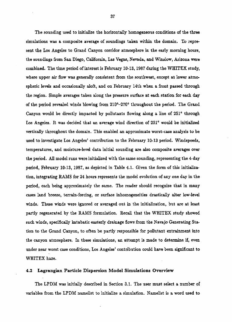
37

The sounding used to initialize the horizontally homogeneous conditions of the three

simulations was a composite average of soundings taken within the domain. To repre­

sent the Los Angeles to Grand Canyon corridor atmosphere in the early morning hours,

the soundings from San Diego, California, Las Vegas, Nevada, and Winslow, Arizona were

combined. The time period of interest is February 10-13,1987 during the WHITEX study,

where upper air flow was generally consistent from the southwest, except at lower atmo­

spheric levels and occasionally aloft, and on February 14th when a front passed through

the region. Simple averages taken along the pressure surface at each station for each day

of the period revealed winds blowing from 2100-2700 throughout the period. The Grand

Canyon would be directly impacted by pollutants flowing along a line of 2510 through

Los Angeles. It was decided that an average wind direction of 2510 would be initialized

vertically throughout the domain. This enabled an approximate worst-case analysis to be

used to investigate Los Angeles' contribution to the February 10-13 period. Windspeeds,

temperatures, and moisture-level data initial sounding are also composite averages over

the period. All model runs were initialized with the same sounding, representing the 4-day

period, February 10-13, 1987, as depicted in Table 4.1. Given the form of this initializa­

tion, integrating RAMS for 24 hours represents the model evolution of anyone day in the

period, each being approximately the same. The reader should recognize that in many

cases land breeze, terrain-forcing, or surface inhomogeneities drastically alter low-level

winds. These winds were ignored or averaged out in the initialization, but are at least

partly regenerated by the RAMS formulation. Recall that the WHITEX study showed

such winds, specifically katabatic easterly drainage flows from the Navajo Generating Sta­

tion to the Grand Canyon, to often be partly responsible for pollutant entrainment into

the canyon atmosphere. In these simulations, an attempt is made to determine if, even

under near worst case conditions, Los Angeles' contribution could have been significant to

WHITEX haze.

4.2 Lagrangian Particle Dispersion Model Simulations Overview

The LPDM was initially described in Section 3.1. The user must select a number of

variables from the LPDM namelist to initialize a simulation. Namelist is a word used to

38

Table 4.1: The sounding used to homogeneously initialize with all height in RAMS simu-lations used in this study. It is a subjective composite of the San Diego, CA, Las Vegas, NV, and Winslow, AZ morning soundings for the 4-day period February 10-13, 1987.

Pressure Height Potential u-component v-component Dewpoint Temperature Wind Wind Depression

(Pa) (m) (K) (m s-l) , (m s-l) (OC) 100000.0 0.0 286.66 2.10 0.80 1.0 85000.0 1354.2 293.38 4.00 1.40 7.4 70000.0 2928.0 301.70 9.20 3.30 12.9 50000.0 5529.5 311.07 13.70 5.00 14.6 40000.0 7157.1 315.58 17.40 6.30 14.6 30000.0 9136.3 320.20 24.40 8.90 40.0 25000.0 10331.1 327.82 27.00 9.80 40.0 20000.0 11772.8 349.57 32.50 11.80 40.0 15000.0 13612.0 371.44 31.50 11.50 40.0 10000.0 16118.2 398.16 18.90 6.90 40.0

5000.0 20301.1 484.94 11.00 4.00 40.0 3000.0 23381.5 560.91 5.40 2.00 40.0 2000.0 25850.3 642.39 4.20 1.50 40.0

describe the file wherein the user inputs the specific data necessary to run the model. The

LPDM was run with the same particle sources for SW-1 through SW-3. The only major

difference, indeed the most important and necessary difference, is that the meteorological

input and surface conditions for each of the three LPDM runs came from the meteorological

output produced by SW-1 through SW-3, respectively. The LPDM runs for SW-1 through

SW-3 are SWP-1, SWP-2, and SWP-3, respectively.

Each of the five LPDM simulations per RAMS run were spawned by a continuous

volume source in the LA Basin at 20 minutes of varying depths vertically and 28.8 km in

the x- and y-directions centered on Los Angeles. One particle is released every 250 seconds

from a randomly selected location within the volume. The turbulence parameterization

within the LPDM (McNider et al., 1988) is turned on such that a turbulent, 3-D, wind

fluctuation is applied to travelling particles. Although no terrain is in SWP-1, both SWP-2

and SWP-3 use the same terrain as exists in the model' domain. For SWP-1 through SWP-

3, LPDM wind fields were interpolated between meteorological fields created at regular

intervals during the 54-hour period.

4.3 SW-l: Simulation Analysis

4.3.1 Meteorological Results: SW-l

39

The meteorological fields that evolve over the 54-hour period from 1200Z to 1800Z (2

days later) generically represent atmospheric conditions in any two days of the composited

period. These fields are depicted in Figures 4.2 through 4.4. Figure 4.2 contains z - z cross

sections through the domain center point of vector wind in four hour intervals beginning

20 hours after run start through 44 hours. Figures 4.3 and 4.4 are the same cross section

but depict the evolution of potential temperature, fJ, and vertical velocity, w, respectively.

Note that winds are very consistent in time and the vertical wind, while developed, is weak.

The potential temperature profile exhibits little change in the upper layers while lower

layers form a 1 km deep unstable boundary layer. This boundary layer begins to develop

significantly between 1200Z and 1800Z and returns to nighttime levels by ..... OOOOZ. The

small depth of the model boundary la:yer is consistent with mid-winter conditions. The

flat terrain of this simulation creates an environment with little forcing; thus winds are

not subject to large change in time. In fact, the only surface inhomogeneity throughout

the domain is the land/sea line along the California coast. Figures 4.5 and 4.6 show

the evolution of horizontal vector winds on an z - y cross section through 73.2 m and

1033.7 m, respectively. As made obvious in the Figures, these winds are quite consistent

throughout the domain in both speed and direction over space and time although evidence

of an inertial oscillation of ..... 20 hours is present. The inertial oscillation period at these

latitudes is, in fact, ..... 20 hours which is consistent with the period of the horizontal

vectors' oscillation. Particles released into such an environment would be expected to

travel in a rather simple manner nearly parallel to the quasi-uniform wind vectors.

40

10.00~----------------~----____________ ~ ____ ~

a 8.001-- - - - - - - - -"- - - - - - - - - --

f----.---- ___ _ - - -" - -~ 6" 00

I- -

N 4.00 f- _ _

r - -

2.00

-1000.00 -500.00 0.00 500.00 1000.00 x (k. m )

10.00~~----------------------------------------~

8.121121- - -. - - - - - ...... - - - - --- - - - - '--

- -~ 6.00

I-

N 4.001-

r - - - - -

2.00

-1000.00 -500.00 0.00 500.00 1000.00 x (k. m )

Figure 4 .. 2: Vertical cross section of vector wind across Grid 1 of SW -1 at ( a) 0800Z, hour 20; and (b) 1200Z, hour 24. The plates are in four-hour intervals beginning 20 hours after run initiation until 44 hours (2 a.m. - 2 a.m. next day). The longest vector represents ..... 27 m s-l.

41

:0 J0~------------------------------------------~ C

8.00

_ 6.00 E ~

N 4.00

2.00

------------------~

-1000.00 -500.00 0.00 500.00 1000.00 x (km)

10.00 d 8.1210 r-- - - - ~ ---+ - - - - - ---+ - - - - - - - ---.

_ 6.00 E ~

r-------------------I- - - -

N 4.00 I- _ _

r -

2.00

-1000.00 -500.00 0.00 500.00 1000.00 x (km)

Figure 4.2: (c) 1600Z, hour 28; and (d) 2000Z, hour 32.

42

10.00~--------~--------------------------------~

~ 6.00 .E

..:c:

e

1--------- ----------

N 4.00 f- _ _ _

f-I- - - - -

2.00 f- - - -

-1000.00 -500.00 0.00 500.00 1000.0121 x (km)

10.00~--------------------------------------~--~

f 8. 012! - - - - - - - - - - - - - - - - - - - -

--------------------~ 6.012!

N 4.1210 f- _

2.00

-100121.1210 -51210.0121 121.121121 51210.0121 1000.0121 x (km)

Figure 4.2: (e) OOOOZ, hour 36; and (f) 0040Z, hour 40.

43

8 .00 - - - - - - - - - - - ------

----------------- --~ 6.00 E ~ -N 4.00 '- _

2.00

-1000.00 -500.00 0.00 500.00 1000.00 x (km)

Figure 4.2: (g) 0800Z, hour 44.

44

a ~.:

4.00

3.50

3.00 300. 300. 300.

~ 2.50 .JJC.

2.00 N 294. 294. 294.

1 . 50

1 . 00

0.50

288. 288. 288.

0.00 -1000.00 -500.00 0.00 500.00 1000.00

x (kml

I-.~ . J0

...., 3.50

3.00 300. 300. 300.

~ 2.50 .JJC.

2.00 N 294. 294. 294.

1 .50

, J0

0.50 288 . 288. 288. .

0.00 -1000.00 -500.00 0.00 500.00 1003.00

x (km 1

Figure 4.3: Same as Figure 4.2 except for potential temperature, (J at (a) 0800Z, hour 20; and (b) 1200Z, hour 24. The lowest 4 km of the 21 km vertical extent of the domain is shown to emphasize boundary layer development. Contour intervals are 1.0°C.

45

r -4.121121

3.5121

3.121121 3"''''. 3"''''. 3"''''. ~ 2.5121 ~

2.121121 N 294. 294. 294.

1 .5121

1 . 121121

121.5121 288. 288. 288.

121.121121 ~

-1121121121.121121 -5121121.121121 121.121121 5121121.121121 1121121121.121121

x (km)

_I 4.121121 U

3.50

3.1210 3"''''. 300. 30"'.

~ 2.5121 ~

2.121121 N 2Q4. 294. 2Q4.

1 .5121

1 . 121121

121.5121

121.121121 ~

-1121121121.121121 -5121121.121121 121.121121 5121121.121121 1121121121.121121

x (km)

Figure 4.3: (c) 1600Z, hour 28; and (d) 2000Z, hour 32.

46

~

1- " 4.00

3.50

3.00 300. 300. 300.

~ 2.50 .J<::

N 2.00 :294. :294. :294.

1 .50

1 .00

0.50

0.00 -1000.00 -500.00 0.00 500.00 1000.00

x (km)

til

4.00 f 3.50

3.00 300. 300. 300.

~ 2.50 ..x:

·2.00 N

:294. :294. :294.

1 .50

1 .00 -0.50

0.00 86. 88. :288.

-1000.00 -500.00 0.00 500.00 1000.00 x (km)

Figure 4.3: (e) OOOOZ, hour 36; and (f) 0040Z, hour 40.

47

4.00 9 3.50

308. 388. 300.

3.00

e 2.50 ..J<::

N 2.00 294. 294. 294.

1 .50

1 .00

0.50 288. 288. 288.

0.00 -1000.00 -500.00 0.00 5eJeJ.00 1000.eJ0

x (km)

Figure 4.3: (g) 0800Z, hour 44.

48

8.00

N

4.00

2.00

-1000.00 -500.00 0.00 500.00 1000.00 x (km)

10.00 b 8.00

~ 6.00 ~

N

4.00

2.00

-1000.00 -500.00 0.00 500.00 1000. 1Zl0 x (km)

Figure 4.4: Same as Figure 4.2 except the evolution of vertical velocity, w at (a) 0800Z, hour 20; and (b) 1200Z, hour 24. Contour intervals are 0.25 cm s-1.

49

10.00

8.00 «::--

N

4.00

2.00

" - , , -

- , .­-' -j

-1000.00 -500.00 0.00 500.00 1000.00 x (km)

112l.12l12l d

2.00

-1000.00 -500.00 0.00 500.00 1000.00 x (km)

Figure 4.4: (c) 1600Z, hour 28; and (d) 2000Z,.hour 32.

.g U'\

'" I

,

' ..

50

8.00

~ 6.00 .:x:.

N

4.00

2.00 ~ __________ ~ ___________ ~0~~

__ ----0~0

-11Zl012l.12l12l -51Zl1Zl.12l1Zl 1Zl.12l12l 51Zl1Zl.01Zl 1000.12l0 x (km)

1 eJ .1Zl1Zl f 8.00

~ 6.1Zl1Zl .:x:.

N

4.00

2.00

-1000.00 -512l0.12l12l 0.00 500.00 1000.00 x (km)

Figure 4.4: (e) OOOOZ, hour 36; and (f) 0040Z, hour 40.

51

H1.00 9

8.00

N

2.00

4.00 6

""--... ~ o

-1000.00 -500.00 0.00 500.00 1000.00 x (km)

Figure 4.4: (g) 0800Z, hour 44.

52

Figure 4.5: The evolution of horizontal vector winds over the 24-hour period 20 hours -44 hours into the simulation in 4 hour intervals at (a) 0800Z, hour 20; and (b) 1200Z, hour 24. This is a plan view on Grid 1 at the first model level 73.2 m above ground level. An inertial oscillation period of ",20 hours is evident. The longest vector represents "'2.8 m S-1.

53

Figure 4.5: (c) 1600Z, hour 28; and (d) 2000Z, hour 32.

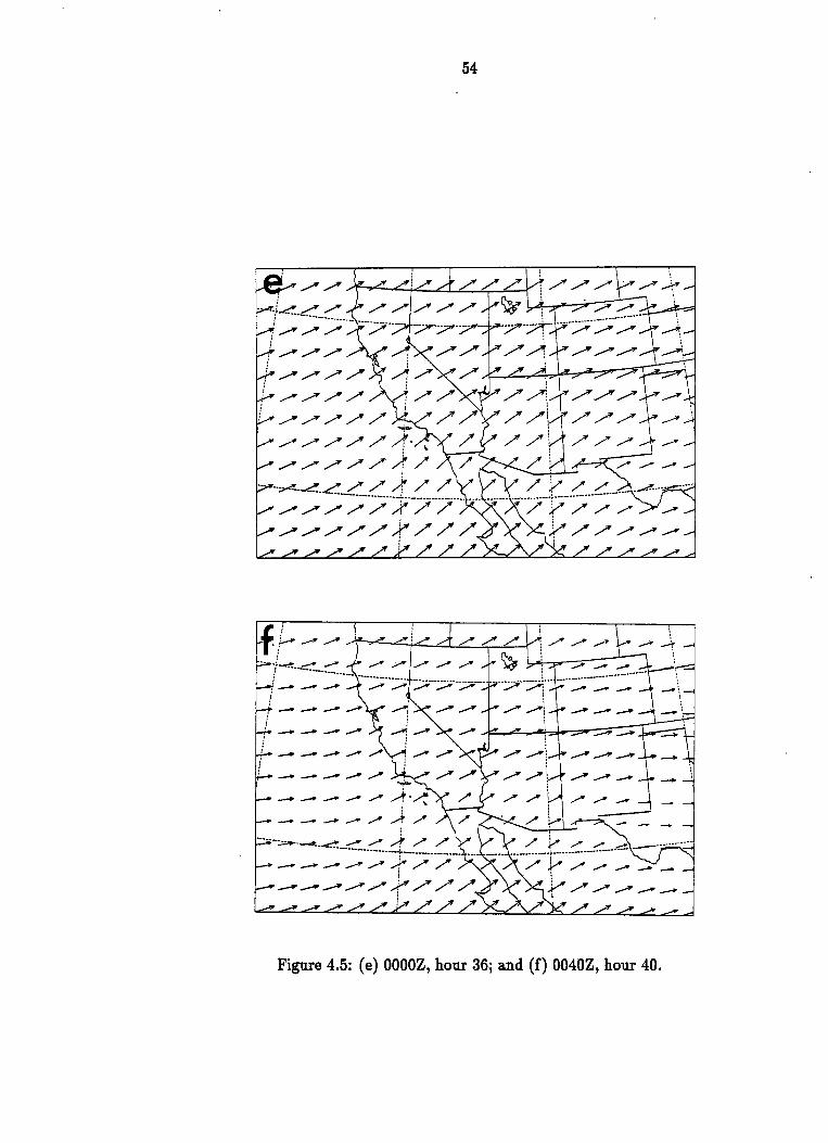
54

Figure 4.5: (e) OOOOZ, hour 36; and (f) 0040Z, hour 40.

It:) It:) \

\ Y' 'i' \ t;, ,!\ \ -~--\---.,--.. \+-\--.-\----, , ,I \ \

, \ , \ \ ,I \ \ I

\ \!\ \ , \ \ \ \ ~ , ,

\ ,/ , \ \ \ \ i , ,

ch--i----~·--·-~·----~-----:--.-.. ~ I:~ J

:t j N o o CO o ,..... bO

'--"

115

""" f! 6'0 ~

56

4.3.2 LPDM Results: SWP-l

As described in 4.2 the Lagrangian Particle Dispersion Model was used to advect par­

ticles representing Los Angeles pollution within the RAMS domain. The 54-hour period

of particle transport was animated on a Stardent console in 210, fifteen-minute incre­

ments. Five distinct particle releases were completed, all centered over Los Angeles. The

five particle simulations are designated SWP-1a through SWP-1e. Their distinguishing

characteristics are:

SWP-1a - A 20 m thick, pancake-like release from the surface (0 m) to 20 m.

SWP-1b - Also a 20 m thick release, but centered around 100 m.

SWP-1c - A 20 m thick release centered on 500 m.

SWP-1d - A 20 m thick release centered on 250 m.

SWP-1e - A 500 m deep volume from the surface to 500 m.

In each simulation one particle was released from within the designated release volume

at the rate of one particle per 250 seconds. By using distinct levels of release, the particular

significance of pollutants at a certain level to the general transport out of the LA Basin

volume was shown. SWP-1e represents the volume of pollutants after accumulating to a

depth of 500 m as generally might exist during stagnant periods such as WHITEX.

As one might expect, a fiat terrain simulation of generically initialized wind conditions

does not reveal much relevant data regarding true dispersion out of the LA Basin. These

simulations are intended to be compared to terrain-inclusive RAMS runs (SW-2 and SW-3)

to evaluate the importance of that terrain.

0-20 m Release: SWP-la

The simulation and subsequent animation of LPDM results for the surface release

reveals considerable vertical mixing but limited horizontal transport (relative to the plume

axis, see Figure 4.7). Because windfields predicted by the model over the homogeneous,

fiat terrain change little throughout the 54-hour period, the LA Basin plume moves in

57

··iM<! /' /' /' /' /' /' /' I ; .. : .. :; ..... -.. ;;. ... ~ ~--;;w···7r-· :

Figure 4.6: Same as Figure 4.5 except for 1033.7 m above ground level at (a) 0800Z, hour 20; and (b) 1200Z, hour 24. The longest vector represents ,....5.0 .m s-l.

c-.i cw:I ,..

;::::I 0

..c:I

N 0 0 0 C"I ..--.. "'t:I "-" "'t:I

fJ ciO

00 1 \1 \ l\ \ \ X \ \1'1rY\ \ ~ 1 \1 \ r\ \ \ V'\ "I", "j,( " " C"I

at)

~ 0

..c:I

N 0 0 CO ...-4 ..--..

U '-'

cO -.io Q) a ~

0 -.:I'

~ 0 ~

N 0 -.:I' 0 0 ......... ..... ......., -d

~ ~

CI:I 1 \1 \ t\ \ \. V\. , k -, ¥ " ,I 1 \ I \ ~ \ \ \7\ "r, ,!I' ,'v ,I C'3 lQ ~

j N 0 0 0 0 .........

cu ......., cO ...;. cu ... eo tZ

60

1~-c.::-~-- __ _ :' -'" -'" -'" :

Figure 4.6: (g) 0800Z, hour 44.

61

the west-southwesterly wind directly toward the Grand Canyon. Figure 4.7, shows the

progression of the plume toward the Grand Canyon at 1, 9, 18, 27, 36, 45 and 54 hours

(13Z day 1 through 18Z two days later). Slight changes in direction from the 2510 wind

(initial) due to inertial oscillation are seen in the slight meander along the plume in time.

Also some shear with height develops in response to surface friction causing the upper

300-500 m of plume to move with a more easterly component with respect to the lower

portion of plume. From the initial release width of approximately 45 km the plume spreads

horizontally to a maximum width of 100 km at simulation end.

Although horizontal dispersion is limited in this stable, wintertime environment, ver­

tical dispersion is limited only by the extent of boundary layer growth. In this simulation

the boundary layer grows to approximately 1 km. Correspondingly, particles initially in

the 0-20 m layer during pre-boundary layer times (overnight) are quickly mixed to 1 km

when ~o boundary layer does form. The animation further reveals that when the bound­

ary layer depth again drops as evening approaches only a small number of particles are

. brought down with it. Particles predominantly remain elevated at the level they achieved

prior to sunset and boundary layer decay. Particles released into the stable overnight

atmosphere do not exhibit significant vertical dispersion, while horizontal dispersion con­

tinues although at a slower rate than during the day. Particles at lower levels move at a

slower rate to the northeast than those aloft.

Under these conditions particles can be counted at different locations to roughly

estimate dilution factors given plume dimensions in the region of interest. Using the

volume containing the first 100 particles for reference, it is found that 100 particles reside

within a volume approximately 5.0 x 104 m x 5.0 x 104 m x 20.0 m. Each particle, then,

represents one-hundredth of the pollutant mass in the LA plume from the surface to 20 m.

At the plume's densest concentration over the Grand Canyon region, 70 particles occupy

a volume approximately 7.0 X 104 m x 1.00 x 105 m x 1.0 x 103 m. The dilution factor

in this case is 200. Although 70% of the original plume pollutant mass transports to ,the

Grand Canyon in the worst instance, the particles disperses through such a great volume

due to natural atmospheric processes that one-two-hundredth of the original concentration

13Z

a , ., . f ,

I !

I I I , , ,

·1~ ! 0

I I

21Z

b

I ... ~t;)I>

I ~

I I

62

Canyon

Canyon

, . , , ,

I \

\ i

\

Figure 4.7: z - y particle position plots for SWP-la from 1 to 54 hours at (a) 1300Z, hour 1; and (b) 2100Z, hour 9. The release area. and Grand Canyon region are labeled and shown as boxes at their respective locations.

63

06Z C

Canyon

15Z

d f

I Canyon

·1~ I ~

I i

Figure 4.7: (c) 0600Z, hour 18; and (d) 1500Z, hour 27.

00Z e

I I I

-1~ I

09Z

f I I I I

I . , , , , I

64

I. . .. :~ . .' . .'

....

Figure 4.7: (e) OOOOZ, hour 36; and (f) 0900Z, hour 45.

,

. , , , , I

, I , , , , , , I ,

, , , ,

I , ,

, , , I , , , II

:

18Z

9 , , , , , , , , , , , , , , , , , , , , , , ,

I I , I

... ~~ ,

I

I !

65

Canyon

Figure 4.7: (g) 1800Z, hour 54.

66

is present. A number of details do not enter into this calculation such as wet and dry

deposition, chemical conversion processes and, likelihood of entrainment into the Grand

Canyon atmosphere (Le. from above th.e inversion in the Canyon). These other effects

would increase the effective dilution factor further. Note that the dilution factor would

have been fifty times less (Le. four, a worst case) if the pollutants had not mixed through

the 1 km deep boundary layer and instead remained within 20 m of the surface. This

emphasizes the importance of the growing boundary layer to the dispersion of pollutant

plumes.

100 m Release: SWP-1b

SWP-1b releases the same pancake of particles centered at 100 m above the surface

over a 20 m depth (90 m - 110 m). Over the 54-hour period many features are the same as

SWP-1a. Because this release begins at a higher altitude its partIcles initially move with

the higher speeds present at that level. However, as the boundary layer grows beyond

100 m depth in the early afternoon, the particles rapidly disperse throughout that depth

just as the 0-20 m release particles of SWP-1a did. SWP-1b appears very much the same

as SWP-1a as depicted in Figure 4.7; its plume meanders with the period of the inertial

oscillation, the dilution factor is r~ughly 200, the primary cause of dilution is boundary

layer growth and the horizontal dispersion of the plume is limited. Very few differences

with SWP-la are seen. The plume mixes more quickly to the top of the boundary layer,

and its leading edge travels slightly faster than SWP-1a. Vertical shear is also evident.

250 m Release: SWP-1c

Just as with SWP-1aand b, SWP-1c transports its plume of 250 m initial elevation

with little horizontal dispersion but with strong vertical mixing. It is also similar in that

the plume meanders with the inertial oscillation of approximately 20 hours and the shear

layers deVelop in time. The leading edge of the plume reaches the Grand Canyon area at 37

hours (7 p.m. MST) just as the sun has set and the boundary layer has reduced in de~th

similar to the plume depiction in Figure 4.7. The leading edge of the plume at 37 hours

is travelling between 800 and 1000 m because it has been subject to (at these heights)

67

to stronger horizontal :O.ow. It is l.ypothesized that such pollutants would not impact the

Grand Canyon due to the stability of the atmosphere during the overnight hours. It would

not be until some 5·8 hours later, when the portion of the plume travelling in the lowest

levels reaches the Grand Canyon area, that an impact would be felt at the surface.

500 m Release: SPW·ld

SWP·ld's release height caused the particle plume to travel slightly more quickly than

the lower level releases SPW·la through c during stable atmospheric periods. Since this

plume was subject to the same boundary layer sequence as all ofSWP·l, its characteristics

of travel in time were very simile.!' to those of SWP-la through c (as depicted in Figure

4.7). For brevity those are listed below:

• Extensive mixing during deep boundary layer periods.

• Little or no mixing overnight and prior to boundary layer growth.

• Shearing with height in tiIIle.

• Leading edge reaches Grand Canyon region at -36 hours. This edge is elevated.

• A slight meander with the geriod equal roughly to an inertial oscillation of 20 hours.

• A dilution factor of apprmdmately 200.

Surface to 500 m Release: SWP-le

As expected SWP-le reveaL; little new information. It contains plume characteristics

of each of the previous simulations except for its uniform, random release appearance

during stable periods due to the nature of its initial configuration. Refer to the description

of SWP-ld for a list of commonalities. During grown boundary layer periods, 1 p.m. -

6 p.m. of each dar, its behavior and appearance are essentially similar to the same time

periods of SWP-la through d alld is well represented by Figure 4.7.

68

4.4 SW-2: Simulation Analysis

4.4.1 Meteorological Results

By adding approximate real topography to the model conditions in SW-2, an attempt

is made to represent the true fields that would exi~lt over the domain. How the model

interpolates the terrain data set to represent actual 1:errain is depicted in Figures 1.3 and

4.8 for Grids 1 and 2, respectively. Note how the model terrain on Grid 2 is more detailed

than that on Grid 1 due to the smaller grid incremelrtt on Grid 2.

Figure 4.8: Topography on Grid 2 for SW-2. Contour intervals are 200 m. Note the additional terrain detail on Grid 2 compared to Grid 1 (Figure 1.3).

Potential Temperature

Figures 4.9 and 4.10 present vertical cross secticms of potential temperature over the

24-hour period from 0080Z to 0800Z the next day (20 nours to 44 hours into the simulation)

on Grid 2 at two different horizontal cross sections (see Figure 4.8 for the extent of Grid

2). Figure 4.11 shows the orientation of these cross sections on Grid 2. Note that by

69

~

a - -330. 330. 1:3

..... , -110.0 320.--.... - 32!1l. 320.

8.0 0 10- -! 6.00

3'0. -- 3'0. 310.

N --4.00 -, 300._ ...... 30!1l.- 3!1l0.

'-t.r... "7'-..... =

.7 "- ~ ""'=="'" F--2Q0. j ~

2.00

::;::::;::0 " -;/, , , I , , , , , I

I , I , , I , , , I , I , , I , I - I , , I I O,00

-600.00 -400.00 -200.00 0.00 200.30 400.00 x (km)

b -- 330 . ..... -10.00 320. __

32!1l. -3211.

8.00 '-

310,- 3'0. 310.

N

4,00

3011.--........ 3110.-300. - -

2.00 - --- -7 \.:: ~ ~ '"---2Q0. -"90

~ ~ --:..

:.-r--;' ,,---.-J 0."''''

-6(;:'1121.0121 -41210. '~121 -21210.00 121 .00 200.0121 4121121 . 121121 x (km)

Figure 4.9: A vertical, z - z cross section of potential temperature, 8, for SW-2 at 120 km north of the domain center point transecting the Grand Canyon for a 24 hr period in 4 hour increments at (a) 0800Z, hour 20; and (b) 1200Z, hour 24. Figure 4.9h is 24 hours earlier than 4.9d for comparisoIL.

70

C 33i!1. -32". ---------32". 32". -

8.121121 "-

~ 6.121121 31". 31".- 31".

N

4.121121

3""·----3"". 3"".

~'\. ..c.s. <:::1 -29". 7 "'~::z.

/ ~ J-.. _J'i

2.121121

121.0121

-612!12!.12!12! -412!12!.12!12! -212!12!.12!12! 121.12112! 212!12!.12!121 412112!.121121 x (km)

1121.121121 d 33". -

32".~ 32". 32". ---8.121121 -"

~ 6. el(21 31". 3'''. 31".

N -4.121121

3"". -------3"". 3"". -2.121121 - Z ~

v'

~~ -

1Z!.1Z!12! -612!12!.12!12! -41210.12!121 -200.12!12! 12! 12!12! 212!12!.0121 41Z!12I.12!12I

X (km)

Figure 4.9: (c) 1600Z, hour 28; and. (d) 2000Z, hour 32.

71

iid.00 e - 33O. --

32O.----- 32O. 32O. ----8.00

! 6.00 310.- 310. 31O.

N

4.00 ~

3oO.-...... 300. 300.

2.00 - ~ -~,,~7

, --

I;;.,-r-j'" ........... 0.00 -600.00 -400.00 -200.00 0.00 200.00 400.00

x (km)

10.00 f- - 330. --320. ------ _ 320. 32O.

8.00

~

! 6.00 310.- 310. 310.

N

4.00 300.-......... 300. 300. ---- - -2.00 ~

".~~ - ~ -----.,....

~ ---I;;.,-r-j'" ~ 0.00 -600.00 -400.~0 -200.00 0.00 200.00 400.00

x (km)

Figure 4.9: (e:) OOOOZ, hour 36; and (f) 0040Z, hour 40.

72

10.00 9 330.

320.- _ - 320. 320.

8.00 f--

! 6 . 00 310. 310. 310.

N

4.00 -300.-- 300. 300.

---. 2.00 -v-

_ .. ~ ~2q0.

i 90.~ ""--""'"

~ ""N. 0.00 -60121.121121 -4121121.121121 -200.1210 121.0121 2121121.00 400.00

x (km)

10.0121 h ~ -- -330. 330.

320. _________ 320. -320.

8.0121

E 6 00 .:L. • ...-

310. ...- 310 . -310.

N -4.00 --. --2.0121

300·~300. 300.

_~L -b t;;..,.-f"'j "'-0.00 -600.00 -40121.00 -20121.1210 0.00 21210.00 4QJ0.0QJ

x (km)

Figure 4.9: (g) 0800Z, hour 44; and (h) 2000Z, hour 8.

73

a ~ 10.00

320. 320. 320.

8.00

310 . 310.-310. E 6 00 .J<:: •

N

4.00

300. 31110. 300.

2.00 -:>

2<l0. ='-- ~ ~- ,<I" ./" -""

0.00 -60ril.0ril -4rilril.rilril -2rilril.rilril ril.0ril 2rilril.rilril 400.00

x (k m )

b -

10.00 320. 320. 320. -

8.00 -~ 6.00 310. 310. 310.

N

4.00

300. 300. 300.

2.00

E--2'1a. ~ .....298. ___ 2'10.-:;::::r

/' .

--r - I

0.00 -600.00 -400.00 -200.00 0.00 200.00 400.00

x (km)

Figure 4.10: A vertical, z - z cross section of potential temperature, 0, for SW-2 at 120 km south of the domain center point transecting the Los Angeles Basin at (a) 0800Z, hour 20; and (b) 1200Z, hour 24. See Figure 4.11 for the cross section locations. The contour interval is 2.0 K, and time interval is 4 hours beginning 20 hours into SW-2 continuing through hour 44.

74

-10.00 r-e -

32f1l. 3211J. 320. -8.00

~ 6.00 31f1l. 310. 31f1l.

N -4.00

30f1l. 300. 300.

2.00

~ 298y _2Cl0.

""" ~ -<:" ~ 0.00

-600.00 -400.00 -200.00 0.00 200.00 400.00 x (km)

10.00 d 320. 32f1l. 320. -

8.00

r-~ 6.00 31f1l. 310. 310.

N

4.00

3011J. 3f1l0. 3f1l0.

2.00 V .... ~ 0.00

-600.00 -400.00 -200.00 0.00 200.00 400.00 x (km)

potential ~emp

Figure 4.10: (c) 1600Z, hour 28; and (d) 2000Z, hour 32.

75

10.00 e -

32121. 32121. 32121.

-8.00

E 6 00 .J<:: • 3113. 31121. 31121 .

I-

N

4.00

30121. 3121121. 3121121.

2.00 Y 29121.

/ -~ - I 0.00 -600.00 -400.00 -200.00 0.00 200.00 400.00

x (km)

potential temp

10.00 .f -

32121. 32121. 32121.

8.00

E 6 00 .J<:: • 3Ull. 31121. 31121.

N

4.00 31219. 3121121. 3121121.

~ 29121.~ ./ 2qOl

Z, -:-0.00

-600.00 -400.00 -200.00 0.00 200.00 400.00 x (km)

Figure 4.10: (e) OOOOZ, hour 36; and (f) 0040Z, hour 40.

76

10.00 .9 -32ril. 32ril. 32ril. -

8.00

! 6.00 31ril. 311l. 31ril.

N

3rilril. 3rilril.- 31lril.

2.00 r---29ril. ~

;;98 .... - 291l./ 7'

/ _. 0.00

,

-600.00 -400.00 -200.00 0.00 200.00 400.00 x (km)

Figure 4.10: (g) 0800Z, hour 44.

77

Gra.nd Ca.nyon

I I I I I I I I

I

I I

\ I

I I

I I I

I

I

\

Figure 4.11: The location of the cross sections depicted in Figures 4.9 (upper horizontal line) and 4.10 (lower horizontal line).

78

1600Z the boundary layer, approximately represented. by the area of vertical isentropes,

has grown to approximately 500 m on the east side of the. mountains. The boundary

layer grows to 1 km by 2000Z and is reduced, as would be expected, into the evening and

overnight hours (OZ - 12Z, next day). This first 24-b.our period (Figure 4.9h) compares

very favorably with the potential temperature fields of the next 24-hour period (Figure

4.9d). The effects of the Pacific Ocean on the boundary layer can be seen in the reduced

depth of the boundary layer throughout the daytime on the west side of the mountains

compared to the high desert (east side of the mounta.ins). For comparison, Figure 4.9h

shows the potential temperature field at 2000Z (2 p.m. MST) but 24 hours earlier than

the 2000Z isentropes in Figure 4.9d. Differences that exist are primarily where expected,

in the lowest 3-4 km of the domain. No direct comparison with observations is strictly

valid because the initial conditions were composited, however, the surface temperatures

are generally within 4°C of actu~ surface temperatures during the WHITEX period.

Horizontal Winds

Wind fields are the single most important variable affecting dry, non-reactive pol­

lutant transport Since moisture fields are not model4!d with microphysics in this study,

the generation of reasonable winds within the simulations is of the greatest importance.

Figure 4.12 depicts the time evolution of horizontal wind vectors for the 24-hour, mid­

simulation period 0080Z - 0080Z, next day, in 4 hour intervals on Grid 2. These are the

near-surface vectors at 73.2 m above the ground on z· surfaces (terrain-following). At

OOOOZ (early evening, 6 p.m. MST) the winds have significantly altered from their initial

west-southwesterly path. This is in stark contrast to the comparatively uniform field over

flat terrain (SW-1, Figures 4.5 and 4.6). The inclus:lon of real terrain to SW-2 has, as

expected, completely changed the windfield evolution. Of course, then, pollutant trajecto­

ries are considerably different when released into SW·2's environment, compared to that

of SW-l. In the northern portion of Grid 2, the severe terrain of the southern Sierra

Nevada mountains have forced impinging winds to diverge to the south causing eventual

convergence with west and southwesterlies in south cEmtral California north of Los Ange­

les (~150 km). This convergence, combined with the relatively high altitude, creates the

79

Figure 4.12: The evolution of horizontal wind vectors on Grid 2 for SW-2 at 73.2 m above ground level for the period 20 hours to 44 hours into the simulation (2 a.m. - 2 a.m. MST) in 4 hour intervals at (a) 0800Z, hour 20; and (b) 1200Z, hour 24. Topography is included in 200 m intervals to better show the effects of terrain. The longest vector represents ",9 m s-1.

80

Figure 4.12: (c) 1600Z, hour 28; and (d) 2000Z, hour 32.

81

Figure 4.12: (e) OOOOZ, hour 36; and (f) 0040Z, hour 40.

82

Figure 4.12: (g) 08~OZ, hour 44.

83

strongest winds, 9.8 m S-l, within the domain at this point. To the east of the California

mountains winds become northerly and even form a counterclockwise circulation just east

of the southern Sierras. Two low-level transport routes appear in the Los Angeles Basin

region. The first follows to the northeast through the region representing Cajon Pass.

The region does not appear as a 'pass' because of the topography smoothing done within

RAMS but is a ridge-like feature. When a fine nest is added over the LA Basin with 8

km grid increment, as in SW-3, such smaller scale features are considerably better repre­

sented. The second route goes through Banning Pass. Both routes have been noted as

pollutant transport routes in previous studies (Ulrickson and Mass, 1990; McElroy, 1987).

In Southern Arizona the initial southwesterly flow has backed to the southeast, ap­

parently due to low-level terrain forcing by the Mogollon and Colorado Plateaus in central

Arizona. This creates a convergence zone in the Mohave desert; a potential location for

pollutant accumulation and circulation. Similar turning of the low-level winds occurs

as southwesterly initial winds impinge on the Cococino Plateau approaching the Grand

Canyon region. Winds become upslope to the elevated land masses. This is noticeable

in Northern Arizona where terrain heights vary (compare wind flows to terrain in Figure

4.12).

At the 1 km level the horizontal wind is, as expected, considerably less influenced by

terrain than at the 73 m level (see Figure 4.13). Some evidence of an inertial oscillation

as was seen in SW-1 appears in SW-2; note the veering of the wind from southwest to

west, particularly at upper levels (as shown by vectors above higher terrain). Maximum

wind speed is maintained well, remaining consistent between 8 m s-l and 11 m s-l once

the model has sufficiently adjusted approximately 6-10 hours into the simulation. Prior

to the adjustment to the idealized initial conditions the wind flows, while consistent in

direction, are higher in speed by 10-40% over the adjusted fields at 12 hours. Note the

consistency between the 1600Z + 2 days (Figure 4.13h) and the 1600Z + 1 (Figure 4.13c)

day horizontal wind vectors. This comparison suggests that the model has developed its

own consistent solution describing how the atmosphere would react to the given terrain,

solar insolation, and idealized initial conditions. Within this regime the pollutant pathways

84

Figure 4.13: Same as Figure 4.12 except for 1033 .. 7 m above ground level at (a) 0800Z, hour 20; and (b} 1200Z, hour 24. The longest vectc'r represents -10 m S-I.

85

Figure 4.13: (c) 1600Z, hour 28; a.nd (d) 2000Z, hour 32.

86

Figure 4.13: (e) OOOOZ, hour 36; and (f) 0040Z, hour 40.

87

Fig-lre 4.13: (g) 0800Z, hour 44.

88

to the northeast and east of Los Angeles are much :.ess distinct. At the height of 1 km

terrain forcing appears to be limited to large-scale vadations in flow. An exception to this

can be found over the severe terrain of the southern Sierra Nevadas where wind vectors

consistently diverge on the mesoscale.

At 3 km (not shown) the terrain influence is even more limited than at the 1 km

level. Model adjustment to terrain effects is limited to approximately a 20% teduction

in initial maximum windspeed. After adjusting, windspeed maxima are approximately 13

m s-1. The inertial oscillation of SW-l and at the 1 km level of SW-2 is further evident

at 3 km. Southwesterly-westerly flow is maintained throughout the simulation to varying

degrees. This level is far less influential on pollutan1 transport due to its altitude above

any anthropogenic source.

Vertical Wind

Figure 4.14 shows the 24-hour evolution of vertical wind, w, from 20 to 44 hours

into the simulation along the LA Basin transect. T:tJ.e simulation is generally character­

ized by weak vertical motion except in mountainous regions where positive and negative

motions peak near 10 cm s-1. As seen in Figure 4.l4 the model is able to simulate the

upward/downward vertical motion couplet typical of mountain-induced gravity waves. On

the mountainside, evidence of upslope flow from solar heating is evident. Pollutants trans­

ported into the mountainous area would become sub.iect to strong mixing and be lifted to

upper levels. That mountainsides are areas of strong ventilation of Los Angeles pollution

has been hypothesized by Ulrickson and Mass (1990a,b), and Segal et al. (1985). Simi­

larly, in the overnight periods, as shown in Figure 4.14a, f, and g shows katabatic mountain

drainage :fiows up to 6 cm s-1. The strength and expa.nse of such vertical motions empha­

sizes the differences in dispersion that are expected to occur between the true terrain and

:fiat terrain simulations. One expects increased dispersion and a lessened impact of Los

Angeles produced pollution on the Grand Canyon simply due to the existence of complex

terrain in the Los Angeles to Grand Canyon corridoJ·.

89

a 112l . I2lI2l

a.0fZ1

E ~ 6.0fZ1

N

4.00

2.00 ~ 1.......1b}

-6I21fZ1. fZll2l -4012l. ~112l -2fZ10. fZll2l fZI. eJl2l 212l12l.00 4QJQJ. 00 x (k. m )

b 112l.fZll2l

-6012l.012l -412l12l.~12l -2012l.12l12l 12l.12l12l 2012l.12l12l 4012l.12l0 x (k. m )

Figure 4.14: The time evolution of vertical motion, w, for SW-2 at the Los Angeles Basin transect for 20 to 44 hours in four hour increments at (a) 0800Z, hour 20; and (b) 1200Z, hour 24. Contours are at 2 em s -1 intervals. This cross section is depicted as the southern horizontal line in Figure 4.11.

90

c 1r2l.r2lr2l

8.r2lr2l

E .J<:: 6. r2lr2l

N

4.r2lr2l

2.r2lr2l

-6r2lr2l.r2lr2l -4r2lr2l.r2lr2l -2r2lr2l.r2lr2l r2l.r2lr2l 2r2lr2l.r2lr2l 40r2l.r2l0 x (km)

d 1r2l.r2lr2l

8.r2lr2l

E .J<:: 6. r2lr2l

4.r2lr2l

2.r2lr2l

-600.00 -40r2l.00 -20r2l.00 0.0r2l 200.0r2l 400.00 x (km)

Figure 4.14: (c) 1600Z, hour 28; ani (d) 2000Z, hour 32.

91

e 10.00

8.00 .) (

"

E ~ 6.00

N

4.00

2.00

-600.00 -400.e0 -200.00 0.00 200.00 400.00 x (km)

10.00

8.00

E ~ 6.00

N

4.00

2.00

-600.00 -400. "0 -200.00 0.00 200.00 400.0121 x (km)

Figure 4.14: (e: 1 OOOOZ, hour 36; and (f) 0040Z, hour 40.

112l.12l12l

8.12l12l

~

E ~ 6.1ZJ12l

N

4.12l12l

2.12l12l

92

Q \:: \ 9 I '0D ~J.:\ , !J;}! 0 /)(1 \$

~ ___ e

. ~~) f '.':f::::--

-612l12l.12l12l -412l12l.12l12l -212l12l.12l12l 12l.12l12l 212l12l.12l12l 412l12l.12l12l

x (km)

Figure 4.14: (g) 0800Z, hour 44.

93

4.4.2 LPDM Results: SWP-2

By running with Lagrangian Pyticle Dispersion Model, using the realistic terrain and

more complicated fields of SW-2, n-lmerous insights into the processes effecting pollutants

transported out of the Los Angeles Basin are found. In comparison to the relatively

simple dispersion characteristics of SWP-1, SWP-2 describes a complicated diurnal cycle

of pollutant flow in the Los Angeles-Grand Canyon corridor.

Similar to SWP-1, SWP-2 ccntains five different types of random volume releases

from within the confines of the Los Angeles Basin. The releases are exactly the same

in dimension as SWP-1 but are elevated somewhat by the inclusion of terrain in SW-2.

As with SWP-1 a rectangular pancake-like volume is the release location for four of the

LPDM runs, its dimensions are ",29 km X ",,29 km x ",,20 m. This rectangular box is

centered on release heights of 10 Il (surface), 100 m, 250 m, and 500 m. A ::fifth run was

completed which extends from 0 In to 500 m in the vertical (representing a deep volume

source). Particle positions were !laved every 15 minutes allowing the animation of 210

consecutive files out to 54 hours. The particle release was begun at 45 minutes into the

simulation and ended at 54 hours with one particle releasing every 250 seconds. A total

of 767 particles were released thrc1ughout each simulation.

0-20 m, 100 m, and 250 m RI!!leases: SWP-2a through SWP-2c

SWP-2a through SWP-2c regesent continuous releases from close to the surface, 100

m and 250 m, respectively. The animation of particle transport over a 54-hour period

reveals numerous atmospheric e:ffl~cts complicating flow out of the LA Basin. Figure 4.15

presents an :c - y view of particle 1;ransport out of the LA Basin in time based on SWP-2e.

Because SWP-2e is a deep release (surface to 500 m) it generically represents the features

that exist in SWP-2a through 2c. For brevity, this figure will be referred to in all SWP-2

discussions ( a-e).

0-4 hours: During this period the model is still adjusting to terrain feature effects and

southwesterlies (all were initialized) exist throughout the domain. Particles

00Z e

. ~.: ..•. .: . ...\ .... ~ ..... . '~·l"'.!o~",,~· .. ···:. : '. -.:,;~\t;.~ .. :.: ..

·i~ ::~;.!" :

! ! i

I · · · I ,

· ·

I r ~ .. t'

I :

96

Canyon .. ".:,'

)::-:'. ":;.~ . ':.'

'0 -0, '':'::-

.\: .

Canyon

Figure 4.15: (e) OOOOZ, hour 36; and (f) 0900Z, hour 45.

I

· · · · · \

\

18Z

9 . . , :

I ..... !. .. • ,,'I ... .,: I

", ~:<. " ':" ";.

0' ••

97

, .. :~ 'I', --.', ·i

.'

...

' .

Grand Ca.nyon

Figure 4.15: (g) 1800Z, hour 54.

· · · · ·

\

98

are trapped within the LA Basin by weak southwest winds which force par­

ticles into the mountains but cannot rke over due to atmospheric stability

prior to boundary layer development.

4-12 hours: The boundary layer grows and decays during this period. Mixing reaches

its maximum and particles are vertic~Jly transported to 800 m or more

where higher horizontal winds take par'dcles over the mountains supported

by upslope :How to the east of LA into the high Mohave desert. Preferred

transport routes are noticeable throug'[ Cajon Pass (which the model to­

pography represents as a low ridge) and Banning Pass, while numerous

particles are also able to travel over th1! mountains of San Bernardino Na­

tional Forest at maximum boundary layer depth.

12-28 hours: During this evening/overnight/early Ilorning period the boundary layer

is reduced in depth and the atmosph3re becomes quite stable. Because

newly released pollutants are, for the most part, trapped within the shallow

boundary layer « 100 m), they reside near the surface and are subject to

low-level, terrain-in:Huenced winds. Particles released in the LA Basin are

brought by easterly land drainage WiIlds to the west (toward the ocean)

away from the Grand Canyon. Once reaching the ocean they converge with

the southwesterlies prevailing there, unaffected by drainage :Hows. This

convergence contains particles along be mountains to the north of LA in

an east-west line. The convergence is weak enough such that the pollutants

remain in low levels. The high desert particles are trapped by atmospheric

stability as well, being subject to a weak anticyclonic desert circulation near

the east side of the San Bernardino National Forest. No particles travel

toward or reach the Grand Canyon in the first 28 hours of this simulation.

28-36 hours: Similar to hours 4-12, this period is th'3 daytime of day 2 where the bound­

ary layer grows to nearly 1 km. Strong mixing takes the once-trapped

particles to upper levels where stron:~er winds are able to advect them.

Particles that were accumulating to the north of Los Angeles quickly rise

99

and move over c,r around the mountains in southwesterly ftow. Newly re­

leased particles in the LA Basin again (similar to hours 4-12) exit to the

Mohave Desert yia Cajon and Banning Passes, predominantly. Particles

which were trap:?ed in the high desert overnight now begin to move again

to the north and east. They do not, however, achieve the Grand Canyon

in large number!:. Instead, since model winds have been forced to become

south-southwestl~rly by terrain and atmospheric physics, the particles move

north passing to the west of the major vistas of the Grand Canyon. Five

of the approximiLtely 100 particles released from the LA Basin during the

previous day crclss the far western edge of Grand Canyon National Park

late in this peric1d. Even so, the height at which they travel, 200-1000 m

above ground le'lel, suggests their entrainment in the Canyon is unlikely

overnight. By nc, means, in this specific study, is the Los Angeles inftuence

able to exceed 0.5% of its initial concentration at the far western end of

the Grand Canyon National Park. The Grand Canyon's primary vistas are

subject to consiC.erably less than 0.5% and are perhaps unaffected.

36-52 hours: This period is quite similar to the 12-28 hour period described earlier, with

the exception of those particles which have traveled to the west and north

of northern Arizclna. While about two-thirds of these particles have become

trapped in the sb.allow overnight boundary layer and travel slowly in the

complex mounta.n flows of eastern California, Nevada, and southern Utah,

another third ar,~ not trapped by the boundary layer. This third travels

at upper levels, where the southwesterlies are consistent and strong. The

particles move with this flow off to the northeast. No additional particles

affect the Grand Canyon.

SWP-2a through SWP-2c nhows that surface LA Basin particles, released to repre­

sent approximate worst-case conditions of ftow toward the Grand Canyon, are strongly

inftuenced by terrain-induced meteorological flows. Terrain effects are so significant at

100

these low levels that dilution is increased to 1000-200(1 from 100-200 for a no-terrain sim­

ulation (see SWP-1 description). This increase in dilution factor is based on the fact that

an order of magnitude fewer particles are able to impact· the Grand Canyon region in

SWP-2a through c. Whereas 70 particles were over GCNP in the worst case of SWP-1,

only 7 particles impacted GCNP in the worst case of :;WP-2. Different estimates of dilu­

tion factors and potential Grand Canyon impact are extended in the SWP-2 discussion.

Furthermore, the terrain slope approaching the Colol~ado Plateau appears to divert ini­

tially west-southwesterly winds away from the Grand Canyon causing plume particles to

avoid the sensitive northern Arizona/Grand Canyon :~egion. It can be speculated that a

meteorological model simulation initialized with low-ll!vel westerly winds instead of west­

southwesterly winds might bring a greater percentagE: of particles to the Grand Canyon.

Such a simulation would not be representative of the WHITEX period, however.

500 m Release: SWP-2d

SWP-2d had considerably different characteristics than the 'boundary layer releases'

SWP-2a through c. The reason for the majority of tbe difference is that the release level

is within the boundary layer for such a short period of time during day 1 of the simulation

that its particles are less terrain-influenced. Figure 4.15 still approximately represents

SWP-2d, however.

More scrutinizing analysis of the potential temperature fields for SW-2 indicates that

the boundary layer on the marine or western side of ttle mountains (the marine boundary

layer) is considerably shallower than the boundary :.ayer elsewhere, especially the high

desert (see Figure 4.10) during daylight hours. Since 3WP-2d releases its particles within

this marine region (on the coast of California), the fact that the marine boundary layer

only exceeds 500 m for a short period (approximately 2 hours) compared to SWP-2a

through c is significant.

During SWP-2d considerable differences arise in the early portion. During the stable

morning period, 0-4 hours of day 1, the particles a:cumulate in the LA Basin, simply

at a higher level than the other releases. In the 4-1:! hour period the particles continue

to accumulate early, until approximately hour six. At this point the boundary layer has

101

grown enough to influence some of the particles. The particles in lower levels are taken up

in boundary layer :fiow and are subject to similar mechanisms as described in the previous

section; they are transported through Cajon and Banning Passes. Where SWP-2d differs

is by the behavior of those particles residing at high levels, above boundary layer effects.

By mid-afternoon, model adjusted fields above the boundary layer (the level of SWP-2d's

release) are more westerly and not subject to upslope effects. This causes the upper­

level SWP-2d particles to travel eastward in more stable, upper-atmosphere layers. These

particles travel at this horizontal level eastward into the desert regions by' early evening

where they accumulate in the lower levels.

Although one might expect the next day to effect the particles of the 500 m release in

the same fashion, it does not. The reason for this appears to be the deeper growth of the

boundary layer during day 2 (28-36 hours). Because the boundary layer grows to 600-700

m on day 2, the particle trans:port on day 2 is essentially the same as that described in

the previous section (SWP-2a-c) for that period.

What are the implications of these differences? What are their causes? The im­

plications are that during WHITEX pollutants which might have accumulated through

stagnation to high levels (Le. 500 m) prior to the event could be transported in large quan­

tities to the eastern portions of the LA Basin. This has little effect on conclusions about

the effect of LA Basin pollutan1;s on the Grand Canyon region, however, because once in

the deep boundary layer of the high desert these particles are transported in southerlies

such that they, too, pass to the west of Grand Canyon National Park. No additional

impact on the Grand Canyon due to their higher release level is found. This may have

caused the boundary layer to grow to a lesser extent on day 1 than day 2.

Surface to 500 m Release: BWP-2e

Because SWP-2e releases particles from all levels from the surface to 500 m, its

characteristics are a combinati,)n of those effects described in the sections for SWP-2a

through d (as shown in Figure 4.15. Although SWP-2e reveals no new information on

impacts of LA Basin pollutants ')n the Grand Canyon, it does represent a different scenario

than SWP-2a-d. By nature of Us configuration, SWP-2e mimics a severe stagnation event

102

~ the LA Basin where pollutants have accumulated unc~er an elevated stable layer to 500 m

in significant concentration. In this case, mixing partic:.es to 1000 m or higher represents a

dilution factor of 2, whereas" the 20 m thick releases (S'VP-2a-d) were subject to a dilution

factor of 50 by the same mixing. SWP-2e represents a.nother level of conservationism in

LA Basin impact assessment which is addressed in thE upcoming discussion of SWP-2.

SWP-2: Discussion

It is seen that pollutants released at essentially a:1Y level near the surface in the LA

Basin in winter conditions are diluted strongly by natural atmospheric processes for this

case study. The dilution process prevents the LA Basin plume from reaching the Grand

Canyon in large concentrations during this simulated period. The actual impact of what

concentration does reach the Grand Canyon during 'VHITEX is implied to be quite low.

Given a dilution factor of 100 (although 200 or higher might more often be found) for a

worst case estimate, and an average LA Basin initial concentration of PM-10 (particles

less than 10 microns) particles of 60 p,g m3-1

, the G)·and Canyon impact could roughly

be 0.6 p,g m3-1

• With mean PM-10 concentrations from March 1988 to February 1991

of approxima.tely 9 p,g m3-1 from th~ National Park Service Fine Particle Network, the

LA Basin contribution to Grand Canyon haze is spe.:ulated to be at most 6.6% during

the February 10-13, 1987 haze period based on this model simulation. Estimates of the

potential impact of LA Basin pollutants on the Grand Canyon with different levels of

dilution are presented in Table 4.2.

Results are presented for boundary layer growth te' 500 and 1000 meters, the 500 meter

assumption being an added measure of conservatism representing the case where the model

predicted boundary layer growth was too great because cloud effects were not represented

in these dry simulations. The worst case surface, wintertime PM-I0 measurement in the

LA Basin (236 p,g m-3 San Bernardino County, CARB, 1986), is divided by a given

dilution factor to determine the p,g m -3 estimated cOllcentration impact of the LA Basin

at the Grand Canyon. The concentration impact is t:~anslated into an estimated percent

impact simply by dividing it by a wintertime PM-10 haze condition measurement in the

Grand Canyon. For the representative haze Grand Canyon measurement, a value of 50

103

Table 4.2: Estimates of Los Anl~eles Basin pollutant impact on Grand Canyon National Park haze conditions during FE!bruary 10-13, 1987 with differencing levels of dilution. The information presented is based on LPDM results for SW-2 and maximum PM-lO concentrations of pollutants of 236 J.Lg/m3 and 50.0 J.Lg/m3 for the LA Basin and the Grand Canyon, respectively. The initial number of particles in all cases was 100.

LPDM Initial Fina, Dilution Final Dilution Total Estimated Run (6) Release PollutE.nt due to # of due to Dilution 'Impact

Depth (m) Depth Vertical Particles Horizontal (%) Mixing Dispersion

SWP-2a-d 20 1000 50 5 20 1000 0.46 20 500 25 5 20 500 0.92

SWP-2e ,500 100e 2 5 20 40 11.8 500 500 1 5 20 20 23.6

J.Lg/m3 i~ used (based on high concentration values in the Grand Canyon, measured by the

Western Fire Particle Network, March 1988 - February 1991). For SWP-2e's 500 meter

deep release into a 1000 meter boundary layer depth, the total dilution is 40. In this case,

the LA Basin impact concentration at the Grand Canyon would be 5.9 J.Lg/m3 • Using the

50 J.Lg/m3 value as representative of typical Grand Canyon haze conditions, the percent

impact of the LA Basin release would be 11.8%.

The calculations presented in Table 4.2 are based on a number of conservative as­

sumptions including: (1) the surface maximum concentration value in the LA Basin (236

J.Lg/m3) is valid from the surfa·:e to 500 m, (2) for the cases where a 500 m final depth

is used, the particles did not mix to the model diagnosed boundary layer depth of ",,1000

meters, (3) wet and dry deposition processes were ignored, (4) each particle reaching

GCNP does become mixed into the Grand Canyon boundary layer and is not transported

away aloft, and (5) chemical cllDversion processes are unimportant. Given these conser­

vatisms and the small magnit11de of the estimated percent impact of the LA Basin on

Grand Canyon concentration, that LA Basin pollutants might be the primary contributor

to WHITEX haze during the February 10-13, 1987 period 'is unlikely.

104

4.5 SW-3: Simulation Analysis

As described previously, SW-3 differs from SW-:! by nature of its nest of 8 km grid

increment over the LA Basin (see Figure 4.1). This allows greater terrain accuracy (Fig-

Figure 4.16: The terrain used on Grid 3 of SW-3. Note the greater detail in this plot com­pared with Figure 4.8 which has 24 km grid increment:!. Cajon Pass shows up considerably better (marked with a C). Banning Pass is marked with a B.

ure 4.16) and far better resolution of mesoscale metEorological processes. Generally, the

inclusion of a fine nest increases the ability of the m:!teorological model, RAMS, to pro­

duce vertical motion. Obviously, this increased motion will affect particle transport as

well. A more accurate picture of the terrain combinHd with the considerably greater at­

mospheric resolution creates significant changes in atmospheric fields compared to SW-2.

These changes will be discussed in the next section. Corresponding changes in particle

transport (SWP-3) are discussed directly after the meteorological results.

105

4.5.1 Meteorological Results: SW-3

Potential Temperature

Figure 4.17 shows the evolution of potential temperature on an x - z plane passing

through the northern part of Ba.nning Pass along the LA Basin transect. By comparing

this cross section to Figure 4.10 of the SW-2 discussion (which transects the same location)

one can see how severely the diffi!rence in grid increment (24 km to 8 km) in the fine grid of

SW-3 effects terrain depiction. ~ote the difference in the representation of the mountain

centered at -175 km in Figure ,1.17 compared to Figure 4.10.

This and other terrain differences induce significant changes in the potential temper­

ature field of SW -3. The primal'Y difference in potential temperature is in the magnitude

of the mountain-induced waves. Note the increased amplitude of the wave induced by the

mountain in the case of SW-3 throughout the time period of Figure 4.18. The evolution

of the boundary layer in SW-3 is very much like that of SW-2. Its depth and location are

nearly identical except in locations where nest differences create differing terrain features.

SW-3 contains more abrupt changes in boundary depth with distan~e as shown in the re­

gion surrounding the mountain in Figure 4.18. Other cross sections show the same ,trends

as described above although tht!y are not shown here.

Horizontal Wind

The horizontal winds in S1.V-3 was quite consistent with SW-2, especially outside of

the finest nest of SW-3. This is to be expected since outside of Grid 3 the grid increment

(and therefore, terrain representation) is identical. A number of changes, however, occur

within the bounds of Grid 3, S'V-3's finest nest. Figure 4.19 presents horizontal wind vec­

tors of SW-3 for Grid 2 during the 24-hour period from 20 to 44 hours into the simulation

at 73.2m. This figure is comparable to Figure 4.12 which shows the same period for SW-2.

Many features are quite similal':

• The convergence line to the north of Los Angeles along the San Gabriel mountains.

• The anticyclone circulation to the east of the southern Sierras.

106

6.00 a - ·306. -_--...I 5.0121

- ------------------------------4.0121{-__________ ------____ ------------______ -1

E

~ 3 . 0121,-.;;...__ ------300 -----... - . r 300. _______ 300.- . N

E

2.1210~ __ --__ ----------~

1 .00 F------~

292.--

~292.~

0.01211~~II~!4~·z~r~~~~~uw~~~L~~~~~LL~ru~ -61210.121121 -4121121.0121 -200.1210 121.1210

6.00 b 5.121121

x (km) 20121.00 400.00

4.001~----------------------------------

:: 3 .121121-1---300. --------300. _-----300.

N

2 . 121121 1--____ ------___ ""-___ .-----292.

1--______ -292.~ . ~

- . 'N""-292. _

1 .00 r:--------, ~-----2S4.

0.121I21'~~~~~yu~~~~uw~~r~~~~~~~~~~

-61210.00 -400.00 -20121.00 121.1210 200.00 400.00 x (km)

Figure 4.17: The evolution of potential tempera.ture f~om 20 to 44 hours of the simula.tion in 4-hour increments on Grid 2 (first nest) for SW-3 en the LA Basin transect. This cross section loca.tion is depicted in Figure 4.11.

107

6.00 C

5.00

4.00

E ~_----300. -------i :: 3.001----300.-~300.-

~------------~ N

-----1 2 .00-1------------- ----- 2<)2.

1----2<)2.--~292.=------.---,

: .00t-_--------------~

6----284.-3.00~~~~~~1~.w~~~~~~~~~~~~~~~~

-600.00 -400.00 -200.00 0.00 200.00 400.00 x (km)

6.00

d 5,00

4,00

E ~ ___ ------300, -----\ :: 3,00t----300.-- -300.

--------------~ N

~--------.-----~-------------------2.00~-----------------

1.00~----------__

~-2e4.-

0.00~~~~~~~~~~~wu~~~~~~~~~~~~

-600.00 -400.00 -200.00 0.00 200.00 400.00 x (km)

Figure 4.17: (,;) 1600Z, hour 28; and (d) 2000Z, hour 32.

108

5. r2lr2J

4.00~ ____________ ~ ______ ----------------11 E __ ---....... __ ---300.----4

::: 3.00 f-----300. "--300.-----------1 N

2.00+-------....-1----292. ---- _--292.

1 .00~-----------~

1=----284. ---. ".00 1 , ! ! ! I I ! I ! I I 1 1 'I! I ! I

-600.00 -400.00 -200.00 0.00 200.00 400.00 x (km)

6.00 f 5.00

4.00~------------______ --------------------------~ E 1------300. ---------300. _------300. ------I

::: 3. r2Jr2J ~--------------~-------N

2.00 ~----

1.001~------------

1------284. __ -:--

12'.0121 I I ! , ! " ! I ! ! I I t 'i I! ! I !

-600.00 -400.00 -200.00 0.00 200.00 400.00 x (km)

Figure 4.17: (e) OOOOZ, hour 36; and (f) 0040Z, hour 40.

109

6.00 9 5.00

F-----31l4. _________ 31l4. -------31l4. -_---J

4.00~ ______________ ------------------------~

E = 3.00~ ______ --------,-____ -------------------j N

~ ___ --296. ------1

~--29c. ----------29b. -- ~ __ -----I 2.001--___ -----

1.00~-----------~1

0.00~~~~~~~~~~~~~~~~~~ww~~~~~

-600.00 -400.00 -200.00 0.00 200.00 400.00 x (km 1

Fil~ure 4.17: (g) 0800Z, hour 44.

E .:z::.

N

110

Ie 5.2 ! .... --

3e4. 3e4. _-----304.

4.0

3.0 --

I -- -296. 296._~

296.-

2.0 -

1.0 288. 288.

J t r "-../ ;.;

- ./ ~ -[II""" 1'1 'I""" r:::G:11 ,~ j j Ii. 0.~

-520.0-450.0-42121.0-3521.0-300.0--250.0-200.0--150.0--100.0 x (k. m )

5.0 Jb -------- ---4.0

3WlWl. 300._ ............... 300.

~ 3.0

N

292. 2q2'-~

92.

2.0

;; V 284. ~

Z , I I I! I I I I I I I I I I I I 'IIIIIIII~ I i j i

1.0

0.0 - 500 . 0-- 450 . 0-- 400 .0- 350.0-- 300 .0--:;: 50 . 0- 200 .0--150 .0--1 00 . 0

x (k. m )

Figure 4.18: The same as Figure 4.17 but for Grid 3 through the LA Basin at (a) 0800Z, hour 20; and (b) 1200Z, hour 24. Note the greater tl!rrain resolution.

111

Ie ----5.21 - - --4.21

3~".

! 3.0 30O, """"---300.

,"J

~

..r---

F 2q2.~ 292,

<'9.?,

2.0

-1 .21

.....,,-~

284,~, ,::L.L , I , , ,

Z.0 -5210. 0-45~. 21-4021,0-350.0-31210.0-25121.0-2121121.0-150.0-1121121.21

x (km)

4.21

EO 3'.0 1-----32il . .L.

___ --30~. ---------32121. -' -_--....J

N ~F ----------------~ 2.0F, __ r 2"2, ---------

1 .0~------------------__

F=-----284

0.2 -I' \ t I , 'i) , , \ ! 'j

'

-52121,0-4521. <l-t;:0, 2-3521.0-3021.0-2521,0-221121.0-15121.0-1121121.121 x (km)

Figure 4.18: (c) 1600Z, hour 28; and (d) 2000Z, hour 32.

E .L

N

112

Ie --5.2 1 4.0 -3.0 320. 303.-------300. -2.2 J"o.

2g2. 2g2·-~2g2. -7

~"""""""" ::~"" ,~~ ..--C

i , I I

1.0

0.2 -5021.0-450. ~.:100. 0-350.0-300. 0-25e. B-200. 0-150.0-100.0

x (km)

5.0 If 4.0 J-------------------------------~--------~

-.L 3. III ~·--300. --------30". -~300.-----!

N

2.0F---------------------------------~~~--____ _J b--------2n. -------292. ---v\..--.... ..

l------------------------------~~ .~/\~~ q2·~ 1.0l :~} ~

~ ..:::= ~ :(:;::::: E :t::::=

SA. 284.

~. 21 ! ! ! ! I \' ! ! ! I 1,1 1 11 ! 1,1 It! I ! I -500.2-450.0-400.0-350.0-300.0-250.0-200.0-150.0-100.0

x (km)

Figure 4.18: (e) OOOOZ, hour 36; and (f) 0040Z, hour 40.

113

5.0 9 --

-r-- -4.0

....... -

E 3.0 .JC. t--3~~. 3i!J0 • -300.

>,J r -2.0

""\...

2Q2. '" 1\: --.,..., Q2 • ......",..-

~. I I I I I I I ' I I I I ' , ,

? ~~ -f~'i·,~~

i !

1 . 0

Z.0 - 502) .0--452. eJ-402l .0-3521 .0- 3eJ0 .0- 250.0- 20e: . 0-1 50.0-100. eJ

x (k.m)

Figure 4.18: (g) 0800Z, hour 44.

114

~,',~-.------~"i~,--'--~~.--------------~~~~~~--------~Ci'~ \loA I .... , ....... ~ ,. : ....

! / \ \, \: ,

,I , 'I ' I ' ~ ~ i ,! , , ·1~

t r

~ r , :'

1

, .... - i' / I, .... 1 '

J ,

~ ; . j

! , : , , , 'I

, ..... : -• .,dt:::.o> , ~[ ~

" i ! ~ !

r , ~'

, , \

/, \

/'. ,/

, / ,

.... \, /,

..... ..... ....... /.

.... -I I

\

\

/'

\ , \ ....

/

/ ,

--r t-

" t i 'l 1 -: ~ j -

\ \ " I \ \

~ \ '

............... - /' \)' ,I

/ .... \- ....

r " , r ", 1 'l 1\ I

'1 ' i 'i -

I \ ~ , \ ~

\ I

, \ ~

, ! I /\ ....

Figure 4.19: Horizontal wind vectors on Grid 2 for SVT·3 at 73.2 m for the 24-hour period between 20 and 44 hours of the simulation at (a) 0800 Z, hour 20; and (b) 1200Z, hour 24. The longest vector represents ",10 m S-I.

, \ .~~

I

'1 I i i : i

it :,

"

'\ ...... , , ... r ,

I

, I

! !

"

115

" /

I /

I / \ .... ! I

... , \ f , "- t r

..... , ,

/ I /

" , /" I

/ ,/ /

! / ,/

! /

I " /

/'

,. ",

,. r ~ 1 'l 1: ' !

'! ' !

'\ -. ~ -.! ' 1\ , \ -~ j -

" ... \ .....

r /' \-" / r / t / t ...- ~ /' -+ / -1 / -1 ... -1

-1 --1 .... 1

Figure 4.19: (c) 1600Z, hour 28; and (d) 2000Z, hour 32.

! r

-'

;- /' -.

Ii • :1::)0>

I ~ ,

! t r ~

i'

- , ~ i' , f'

............ 1

-+ i -r--

1-. ,i \ i

i

'i ·d1::)o>

oJ .

1 i r r , I'

116

, ~

/' ./ \ \

\ /' ! ,

"-I

). -- " , \

/- I \ . \

- f ! /' t -, - ;- \

, ~

/' 1 /' /' , /\ I " ,

" ../.:. " ~

,.,.

'" " _I

"- \ "-./

'- "-///

-""-! ,- , I

I

/

,/ -,/ /' /' :" " /' ,/ /',/ /' /' ~

r" ./ /' /'" " /' r /' ./ /'" , ,- t-,- ,/ /' / /' ./ t I I ,/ // ,/ ~ ! " ,/ ,/ /' /~

I I I ,/ /' 1-I 1 " " " i 1 1 " ;- -r 1 " -' i

/' .-" -t -i

/' -- -1

/' /' .... -- - .... ; .....

" - - - -l--- ,.,. i

-- i-'

~ ~ '" / f 1 /' /' - r ,.,. -- ~ +

.... -- i i - '" i

- -\ - ..... \ .....

- '\ " '\

Figure 4.19: (e) OOOOZ, hour 36; and (f) 0040Z, hour 40.

117

'" \

~ \ -,.. - ~

\ "

"- " - " "- ....

/-

" -. ,

'"

Figure 4.19: (g) 0800Z, hour 44.

- ..... ... -

-' /"

....

i i-

t '1 ,\ ~! "\ -

i I 1 \ . ;

: -;

118

• The turning of the wind away from the Colorado Plateau in eastern Arizona.

• The consistency of southwesterly flow over the 30uthwestern part of the Grid 2

domain.

• The maximum windspeed averages only 0.6 m s-l less than that of SW-2 during the

24-hour period (10.2 m s-l for SW-3 vs. 10.8 m S-l for SW-2).

Differences arise for the most part within or near the Grid 3 area. Winds over the ocean

back more in SW-3, being more southerly than SW-2 a"; the similar times.

The strength of the convergence along the San Gabriel mountains increases in SW-3.

Divergence of winds around the better resolved moun1.ains of San Bernardino National

Forest is considerably more evident, as is convergence into Cajon Pass. Within Grid 3 in

the LA Basin over land, windspeeds drop somewhat, approaching 0 m S-l in one location.

At 1033 m (not shown) the horizontal winds in SW-3 are consistently southwest

throughout the simulation period of 54. Although not ;hown, a southerly"wind develops

along the California/Arizona border and to the west of the Sierras which lasts throughout

the simulation. This feature is consistent between SW·3 and SW-2. For the most part,

differences (and even these are small) exist over the Grid 3 area. Slight directional differ­

ences appear in time reflecting the model's adjustment to the better terrain resolution in

Grid 3. For instance, at 1200Z winds in the LA Basin fer SW-3 appear to be considerably

more diverted by terrain, in this case the San Bernardino National Forest region, than in

SW-2. Also, between 1600Z and 2000Z in SW-3, LA Be.sin winds drop from 3-4 m S-l to

0-2 m S-l whereas in SW-2 winds drop to 2-3 m s-l fo:~ the same period.

At approximately 3 km terrain influence drops off considerably. In fact, velocity

differences between SW-3 and SW-2 are quite limited alLd hardly detectable at this height

over the simulation period. Over the 24-hour period (2)-44 hours of the simulations) the

maximum windspeed of SW-3 is 0.17 m s-l higher than SW-2, while vector direction

differences are negligible.

119

8.00

E ~ 6.0(2)

4.00

2.021

-600.00 -40e.00 -200.012J 0.12J0 200.00 400.00 x (km 1

10.l2lfl)

8.00

E ~ 6.00

N

4.021

2.00

-61Zl1Zl.1Zl1Zl -41Zl" .1Zl1Zl -21Zl1Zl.00 0. 01Zl 20(2) .00 40rzJ . 00 x (kml

Figure 4.20: Vertical motion for SW-3 at +120 km on Grid 2 for hours 20 to 44 into the simulation in 4 hour increm.mts at (a) 0800Z, hour 20; and (b) 1200Z, 'hour 24. This passes through the Grand Cc.nyon region. The contour interval is 3 cm s-l.

120

c 10.00

8.00

\~~ o 121

N

4.00

2.00

-600.00 -400.00 -200.00 0.00 200.00 400.00 x (km)

-E

...:: 6.00

N

4.00

2.00

-600.00 -400.00 -200.00 0.0~ 200.00 400.00 x (km)

Figure 4.20: (c) 1600Z, hour 28; and (d) 2000Z, hour 32.

121

-MH!J . 00 -400. ~10 -200.00 0.00 200.00 400.01Zl x (km)

8.0eJ

-E

.:.::. 6.00

N

4.00

2.1Zl1Zl

-6eJ0.0eJ -400.eJ0 -20eJ.eJ0 eJ.eJ0 2eJeJ.0eJ 4eJeJ.lZleJ x (km)

Figure 4.20: (e) OOOOZ, hour 36; a.nd (f) 0040Z, hour 40.

122

9 1eJ.eJeJ

8.eJeJ

N

4.eJeJ

2.eJeJ

-6121121 .121121 -4eJl2J .l2JeJ -2121121 .121121 121 .l2JeJ 2eJQJ . eJeJ 4eJ0 . eJeJ x (km)

Figure 4.20: (g) 0800Z, hour 44.

E ~

N

123

a 'v\.,J 1J.0

8.0

6.0

4.0 f> e...,.../

2.0

-5012l .0-450.0-4 2112l. 0-350 . 0-312l0 . 0-2512l . 0-212l0. 0-150. 0-112l12l .0 x (km)

10.0 b 8.12l

~ 6.0

N

4.0

2.0

-500. 0-450.0-L·00. 0-350. 0-300. 0-250. 0-200. 0-150. 0-100.0 x (km)

Figure 4.21: Vertical motion for SW·3 at -120 km on Grid 3 for hours 20 to 44 in 4 hour increments at (a) 0800Z, hour 20; and (b) 1200Z, hour 24. This passes through the LA Basin and Banning Pass. The contour interval is 5 cm 8-1.

E ~

N

E ~

N

124

8.0

6.0

4.0

2.0

-500.0-450.0-400.0-350.0-300 . QJ-2~i0. 0-200.0-150.0-100.0 x (km)

10.0

8.0

6.0

4.0

~ 2.0

-500.0-450. QJ-400. 0-350.0-300. QJ-2~i0. 0-200.0-150.0-100.0 x (km)

Figure 4.21: (c) 1600Z, hour 28; and (d) 2000Z, hour 32.

125

10.0

8.0

..2 6.0

-E

.::L -N

4.0

2.0

-500.0-450.0-400.0-350.0-300.0-250.0-200.0-150.0-100.0

x (km)

10.0 f

8.0

6.0

4.0

2.0

___ 0.0

-500.0-450. 0-40~. 0-350.0-300.0-250.0-200.0-150.0-100.0

x (km)

Figure 4.21: (Il) OOOOZ, hour 36; and (f) 0040Z, hour 40.

E .x.

N

126

10.0 9 ~.~) (

lSI

lSI

8.0

6.0

4.0

2.0

~

-500 .12l-4512J .12l-412J0 .12l-35eJ .12l-3012J .12l-2'50 .12l-200 .12l-150 .12l-1 r2Jr2J. r2J

x (km)

Figure 4.21: (g) 0800Z,tlour 44.

127

Vertical Wind

Vertical wind profiles for SV\'-3 on Grids 2 and 3 are shown in Figure 4.20.

The additional capability of RAMS to resolve vertical motion with decreasing grid

increment can easily be seen by comparing 4.20 and 4.21. Note the strength differences;

on Grid 2 the magnitude of the largest vertical motion is 8 cm S-1 at 1600Z, on Grid 3 the

maximum magnitude at 1600Z is 30 cm s-l. Obviously, such differences are important

with respect to pollutant transport. Larger vertical motions not only increase the depth

of the boundary layer but bring 110llutants to higher levels in the atmosphere subjecting

them to higher horizontal windsp eeds as well.

Concentrating on Grid 3 (Figure 4.21) because the Grid 2 vertical motion analysis

is much the same as that for SW-2, what mesoscale meteorological attributes are better

represented by Grid 3 in relation to w? The most noticeable difference is the strength ofthe

mountain-induced downward/upward vertical motion couplet. The finer scale evolution

of this feature is evident in time to an extent unresolved in SW-2 on Grid 2. Also easily

seen is the diurnal cycle of upsll)pe heating on the mountainside. Note in Figure 4.21

that the morning hours (1200Z lIld 1600Z) show little or no vertical motion along the

mountain, but by 2000Z (2 p.m.) strong upslope ascent of 20 cm s-1 has formed on

the western slope and upslope cc.used upward motion of 10 cm S-1 on the eastern slope.

Toward sundown (sun shining on western slope only) at OOOOZ upslope only remains

on the western slope having wea.kened to an ascent of 15 em s-l. The eastern slope's

upslope has reversed and becomE: downslope; perhaps combining with the mountain wave

on the eastern side to create strc1ng descent of 30 cm s-l. Overnight the western upslope

deteriorates completely; the eastern side downslope is more persistent, lasting until early

morning when the eastern side atmosphere has so stabilized that the mountain induced

downslope has stopped. Note thc.t the upslope regime lasts only 6 hours during the highest

sun during these winter conditions.

4.5.2 LPDM Results: SWP-3

As with SW-l and SW-2, Hve simulations of particle transport were completed for

SW-3, SWP-3a through SWP-3H. The five runs of SWP-3 were identical in configuration

128

to the previous LPDM runs with an area release of 20 m depth for a) surface, b) 100 m,

c) 250 m, d) 500 m, and a volume release e) extending from the surface to 500 m. Since

these runs are exactly similar to the previous LPDM runs in configuration, the in:fluence

of increased terrain and meteorological resolution of SW-3 is shown by this analysis.

Because of the higher resolution on GrId 3 of S'V-3 mesoscale motions were better

represented. The resulting fields were more complex and contained distinctly stronger

vertical motions than SW-2. Particle model analysis 0:: SWP-2 revealed the importance of

vertical motion to particle transport, particularly in zeference to boundary layer mixing.

The meteorological differences between SW-3 and SV/-2 manifest themselves as particle

transport details in SWP-3. More specifically the pa.rticle simulations of SW-3, SWP-

3a-e, vary in large part by the vertical placement of particles in time compared to those

of SWP-2. This, in tum, creates minor differences in horizontal position generally, with

major differences on occasion. As with the SWP-2 d.scussion for brie:fly only OI).e figure

representing the time evolution ofthe surface to 500 m release (in this case, SWP-3e) will

be referred to throughout the upcoming discussion (Figure 4.22). In essence, the SWP-3

set of simulations maintains the general pat,terns of S WP-2. For this reason, as with the

earlier descriptions, only differences will be emphasized, and the set of five simulations are

grouped together in the discussion.

The animation of the 54-hour period of continu)us particle surface release for the

LA Basin reveals the numerous effects of Grid 3 on particle positions in time. Many

of the main features seen in SWP-2 are found in S\VP-3a, as seen in Figure 4.22. The

following were repeated in a general sense: 1) trapping of pollutants in the LA Basin and

the high desert during stable atmospheric periods with low wind :flow, 2) katabatic :flows

transporting pollutants westward to converge with southwesterly winds over and near the

ocean, 3) mixing of particles deep within the boundary layer of Los Angeles allowing

transport through passes and over mountains, 4) mixing of particles in the deep, high

desert boundary layer to the point where they are cat.ght in stronger, southerly winds at

higher altitudes, and 5) the lack of significant numbers of particles crossing Grand Canyon

National Park boundaries.

13Z a

21Z

b

I

I

·1~ I

129

Canyon

Canyon

, . , . , , , , , , , · , , , , , ,

· , · , , , , , , , , , , · , , , , · , · · , · · ·

\

, , , · ,

· · , , · , · · , , , , , , , , , · , , , , , , · , , , ·

I

\

Figure 4.22: The time evolution of particle positions for SWP-3e from 1 to 54 hours (a)

1300Z, hour 1; and (b) 2100Z, b.our 9. Note the greater detail compared to Figure 4.15.

06Z C

I ,

, , , , ,

I

~1~

15Z

d

! I !

, , , , , , , ,

I I I I I

~1~ i

I

130

Canyon

;.: Grand Canyon

.....

.. - ~ . . '

Figure 4.22: (c) 0600Z, hour 18; and (d) 1500Z, hour 27.

, , , , , , , , I

, , , , , , , i

\

\

\ \

\

\

00Z e

I

I

I

I I I I I I

I I

I :

I I

I

... octb<>

09Z

f

I co

! I ! :

I I I

"'1~ i co

I !

131

.1 Canyon

Grand Canyon

.....

Figure 4.22: (e) OOOOZ, hour 36; and (f) 0900Z, hour 45.

· I I I I

· , I · I

· I · · I

\

\

18Z

9 ! {

J

I . t

f , , , --tit:»

I ~ i !

I

132

,.:' .. ::

Grand Canyon

. Figure 4.22: (g) 1800Z, Itour 54.