the polarcat model intercomparison project (polmip

Atmos. Chem. Phys., 15, 6721–6744, 2015

www.atmos-chem-phys.net/15/6721/2015/

doi:10.5194/acp-15-6721-2015

© Author(s) 2015. CC Attribution 3.0 License.

The POLARCAT Model Intercomparison Project (POLMIP):

overview and evaluation with observations

L. K. Emmons1, S. R. Arnold2, S. A. Monks2, V. Huijnen3, S. Tilmes1, K. S. Law4, J. L. Thomas4, J.-C. Raut4,

I. Bouarar4,*, S. Turquety5, Y. Long5, B. Duncan6, S. Steenrod6, S. Strode6,21, J. Flemming7, J. Mao8, J. Langner9,

A. M. Thompson6, D. Tarasick10, E. C. Apel1, D. R. Blake11, R. C. Cohen12, J. Dibb13, G. S. Diskin14, A. Fried15,

S. R. Hall1, L. G. Huey16, A. J. Weinheimer1, A. Wisthaler17,18, T. Mikoviny17,18, J. Nowak19,**, J. Peischl19,

J. M. Roberts19, T. Ryerson19, C. Warneke19, and D. Helmig20

1Atmospheric Chemistry Division, National Center for Atmospheric Research, Boulder, CO, USA2Institute for Climate and Atmospheric Science, University of Leeds, Leeds, UK3Royal Netherlands Meteorological Institute (KNMI), De Bilt, the Netherlands4Sorbonne Universités, UPMC Univ. Paris 06, Université Versailles St-Quentin, CNRS/INSU, LATMOS-IPSL, UMR8190,

Paris, France5Laboratoire de Météorologie Dynamique, IPSL, CNRS, UMR8539, 91128 Palaiseau CEDEX, France6NASA Goddard, Atmospheric Chemistry and Dynamics Laboratory, Code 614, Greenbelt, Maryland, USA7ECMWF, Reading, UK8NOAA GFDL and Princeton University, Princeton, NJ, USA9Swedish Meteorological and Hydrological Institute, 60176 Nörrkping, Sweden10Environment Canada, Downsview, Ontario, Canada11Department of Chemistry, University of California-Irvine, Irvine, CA, USA12Chemistry Department, University of California-Berkeley, Berkeley, CA, USA13University of New Hampshire, Durham, NH, USA14NASA Langley Research Center, Chemistry and Dynamics Branch, Hampton, VA, USA15University of Colorado, Boulder, CO, USA16Georgia Institute of Technology, Atlanta, GA, USA17University of Innsbruck, Innsbruck, Austria18University of Oslo, Oslo, Norway19NOAA Earth System Research Lab, Boulder, CO, USA20INSTAAR, University of Colorado, Boulder, CO, USA21Universities Space Research Association, Columbia, MD, USA*now at: Max Planck Institute for Meteorology (MPI-M), Hamburg, Germany**now at: Aerodyne Research, Inc., Billerica, MA, USA

Correspondence to: L. K. Emmons ([email protected])

Received: 30 October 2014 – Published in Atmos. Chem. Phys. Discuss.: 26 November 2014

Revised: 20 March 2015 – Accepted: 27 May 2015 – Published: 17 June 2015

Published by Copernicus Publications on behalf of the European Geosciences Union.

6722 L. K. Emmons et al.: POLMIP overview

Abstract. A model intercomparison activity was inspired by

the large suite of observations of atmospheric composition

made during the International Polar Year (2008) in the Arc-

tic. Nine global and two regional chemical transport models

participated in this intercomparison and performed simula-

tions for 2008 using a common emissions inventory to assess

the differences in model chemistry and transport schemes.

This paper summarizes the models and compares their sim-

ulations of ozone and its precursors and presents an eval-

uation of the simulations using a variety of surface, bal-

loon, aircraft and satellite observations. Each type of mea-

surement has some limitations in spatial or temporal cov-

erage or in composition, but together they assist in quanti-

fying the limitations of the models in the Arctic and sur-

rounding regions. Despite using the same emissions, large

differences are seen among the models. The cloud fields and

photolysis rates are shown to vary greatly among the mod-

els, indicating one source of the differences in the simulated

chemical species. The largest differences among models, and

between models and observations, are in NOy partitioning

(PAN vs. HNO3) and in oxygenated volatile organic com-

pounds (VOCs) such as acetaldehyde and acetone. Compar-

isons to surface site measurements of ethane and propane in-

dicate that the emissions of these species are significantly

underestimated. Satellite observations of NO2 from the OMI

(Ozone Monitoring Instrument) have been used to evalu-

ate the models over source regions, indicating anthropogenic

emissions are underestimated in East Asia, but fire emissions

are generally overestimated. The emission factors for wild-

fires in Canada are evaluated using the correlations of VOCs

to CO in the model output in comparison to enhancement fac-

tors derived from aircraft observations, showing reasonable

agreement for methanol and acetaldehyde but underestimate

ethanol, propane and acetone, while overestimating ethane

emission factors.

1 Introduction

Observations show that the Arctic has warmed much more

rapidly in the past few decades than global-mean temperature

increases. Arctic temperatures are affected by increased heat

transport from lower latitudes and by local in situ response

to radiative forcing due to changes in greenhouse gases and

aerosols (Shindell, 2007). Model calculations suggest that in

addition to warming induced by increases in global atmo-

spheric CO2 concentrations, changes in short-lived climate

pollutants (SLCPs), such as tropospheric ozone and aerosols

in the Northern Hemisphere (NH), have contributed substan-

tially to this Arctic warming since 1890 (Shindell and Falu-

vegi, 2009). This contribution from SLCPs to Arctic heat-

ing and efficient local amplification mechanisms (e.g., ice-

albedo feedback) put a high priority on understanding the

sources and sinks of SLCPs at high latitudes and their cli-

matic effects. Despite the remoteness of the Arctic region,

anthropogenic sources in Europe, North America and Asia

have been shown to contribute substantially to Arctic tropo-

spheric burdens of SLCPs (e.g., Fisher et al., 2010; Sharma

et al., 2013; Monks et al., 2014; Law et al., 2014). The Arc-

tic troposphere is more polluted in winter and spring as a re-

sult of long-range transport from northern mid-latitude con-

tinents and the lack of efficient photochemical activity or wet

scavenging needed to cleanse the atmosphere (Barrie, 1986).

Large forest fires in boreal Eurasia and North America also

impact the Arctic in the spring and summer seasons (Sode-

mann et al., 2011). Our understanding of contributions from

SLCP sources to present-day Arctic heating is sensitive to

the ability of models to simulate the transport and processing

of SLCPs en route to the Arctic from lower latitude sources.

This model skill has implications for our confidence in pre-

dictions of Arctic climate response to future changes in mid-

latitude anthropogenic and wildfire emissions.

Comparisons of model results to long-term surface ob-

servations have shown that global chemical transport mod-

els (CTMs) have notable limitations in accurately simulat-

ing the Arctic tropospheric composition, as well as having

significant differences among models (e.g., Shindell et al.,

2008). Transport of emissions from lower latitudes to the

Arctic is mainly facilitated by rapid poleward transport in

warm conveyor belt airstreams associated with frontal sys-

tems of mid-latitude cyclones (Stohl, 2006). The result is that

although the Arctic is remote from source regions, Arctic en-

hancements in trace gas and aerosol pollution are far from

homogeneous. They are instead characterized by episodic

import of pollution-enhanced air masses, exported from

the mid-latitude boundary layer by large-scale advection in

frontal systems (Sodemann et al., 2011; Schmale et al., 2011;

Quennehen et al., 2012). Polluted air uplifted from warmer,

southerly latitudes (Asia and North America) tends to en-

ter the Arctic at higher altitude, while air near the surface

is influenced mainly by low-level flow from colder, more

northerly source regions, particularly Europe (e.g., Klonecki

et al., 2003; Stohl, 2006; Helmig et al., 2007b; Tilmes et al.,

2011; Wespes et al., 2012). The stratification of the large-

scale advection and slow vertical mixing leads to fine-scale

layering and filamentary air mass structure through the Arctic

troposphere, where air masses from different source origins

produce distinct layers, and are stirred together only in close

proximity, while mainly retaining their own chemical signa-

tures (Engvall et al., 2008; Schmale et al., 2011). Air masses

are eventually homogenized by turbulent mixing and radia-

tive cooling, but usually on timescales longer than the rapid

advection along isentropic surfaces that is characteristic of

intercontinental transport in these systems (Methven et al.,

2003, 2006; Stohl, 2006; Arnold et al., 2007; Real et al.,

2007). For global Eulerian models, representing this fine-

scale structure, subsequent slow mixing and chemical pro-

cessing is challenging, particularly with characteristic coarse

grid sizes of 100 km or more.

Atmos. Chem. Phys., 15, 6721–6744, 2015 www.atmos-chem-phys.net/15/6721/2015/

L. K. Emmons et al.: POLMIP overview 6723

A large suite of observations was collected during the

International Polar Year (IPY 2008) as part of the inter-

national POLARCAT (Polar Study using Aircraft, Remote

Sensing, Surface Measurements and Models, of Climate,

Chemistry, Aerosols and Transport) activity (Law et al.,

2014). Numerous papers have been written on these ob-

servations and corresponding model simulations (many are

in a special issue of Atmospheric Chemistry and Physics;

http://www.atmos-chem-phys.net/special_issue182.html).

The POLARCAT Model Intercomparison Project

(POLMIP) was organized with the goal of exploiting this

large data set to comprehensively evaluate several global

chemistry models and to better understand the causes of

model deficiencies in the Arctic. While aerosols are an im-

portant component of the Arctic atmospheric composition,

POLMIP focuses on gas-phase chemistry, primarily carbon

monoxide (CO), reactive nitrogen (NOy), ozone (O3) and

their precursors. This paper provides an overview of the

POLMIP models and their evaluation against observations,

as well as an evaluation of the emissions inventories used

by the models. Two additional papers present more detailed

analyses (Monks et al., 2014; Arnold et al., 2014). Monks

et al. (2014) comprehensively evaluate the model CO and O3

distributions with surface, aircraft and satellite observations

as well as compare the effects of chemistry and transport

using synthetic tracers. In general, the models are found to

underestimate both CO and O3, while the modeled global

mean OH amounts are slightly higher than estimates con-

strained by methyl chloroform observations and its emission

estimates, suggesting the model errors are not entirely

due to low emissions. The comparison of fixed-lifetime

tracers to idealized OH-loss CO-like species shows that

the differences in OH concentrations among models have

a greater impact on CO than differences in transport in

the models. The tracer analysis also shows a very strong

influence of fire emissions on the atmospheric composition

of the Arctic. Ozone production in air influenced by biomass

burning is evaluated by Arnold et al. (2014). Using tracers

of anthropogenic and fire emissions, fire-dominated air was

found to have enhanced ozone in the POLMIP models, with

the enhancement increasing with air mass age. Differences

in NOy partitioning are seen among models, likely due to

model differences in efficiency of vertical transport as well

as hydrocarbon oxidation schemes.

The next section of this paper gives an overview of the

POLARCAT aircraft campaigns that prompted this intercom-

parison (Sect. 2). Section 3 presents a summary of the mod-

els that participated, along with a description of the model

experiment design and the emissions used. Comparisons of

the model results with observations are shown in Sect. 4, in-

cluding vertical profiles of ozone from sondes, surface layer

non-methane hydrocarbons (NMHCs), satellite observations

of NO2, and the numerous compounds measured from re-

search aircraft. Finally, an evaluation of fire emission fac-

tors is shown in Sect. 5, using aircraft observations of fire-

influenced air masses.

2 POLARCAT observations

POLARCAT is a consortium of tropospheric chemistry ex-

periments performed during the IPY 2008 (Law et al., 2014).

A wealth of data on tropospheric ozone and its photochem-

ical precursors were obtained through the depth of the Arc-

tic troposphere during spring and summer. These observa-

tions provide an opportunity to evaluate model represen-

tations of processes controlling tropospheric ozone in im-

ported pollutant layers above the surface. The NASA Arctic

Research of the Composition of the Troposphere from Air-

craft and Satellites (ARCTAS) mission (Jacob et al., 2010)

was grouped into three parts, ARCTAS-A, ARCTAS-B and

ARCTAS-CARB. Three research aircraft took part in this

campaign with a slightly different goal for each mission.

ARCTAS-A and ARCTAS-B targeted mid-latitude pollution

layers and wildfire plumes, respectively, transported to the

Arctic. ARCTAS-CARB was focused on California air qual-

ity targeting fresh fire plumes in northern California, as well

as various anthropogenic sources (Huang et al., 2010; Pfister

et al., 2011).

The NOAA Aerosol, Radiation, and Cloud Processes af-

fecting Arctic Climate (ARCPAC) mission was conducted

in spring between the end of March and 21 April using the

NOAA P3 aircraft (Brock et al., 2011). It was designed to

understand the radiative impacts of anthropogenic pollution

and biomass burning. The campaign was based in Fairbanks,

Alaska, and frequently targeted wildfire plumes that were

transported from Siberia (e.g., Warneke et al., 2009).

POLARCAT-France, using the French ATR-42 aircraft,

was based in Kiruna, Sweden, and took place between

30 March and 11 April (de Villiers et al., 2010; Merlaud

et al., 2011). The summer mission was based in western

Greenland in Kangerlussuaq and took place between end of

June and mid-July (Schmale et al., 2011; Quennehen et al.,

2011).

The POLARCAT-Greenland Aerosol and Chemistry Ex-

periment (GRACE) mission was conducted during the same

time (1–17 July), based also at Kangerlussuaq, Greenland,

using the DLR Falcon research aircraft (Roiger et al., 2011).

Flights covered latitudes from 57 to 81◦ N and targeted an-

thropogenic and fire emissions in the troposphere and lower

stratosphere.

YAK-AEROSIB (Airborne Extensive Regional Observa-

tions in Siberia) was conducted in July 2008 covering parts

of northern and central Siberia using an Antonov-30 research

aircraft, operated by the Tomsk Institute of Atmospheric Op-

tics (Paris et al., 2008). This campaign was also performed

in collaboration with the POLARCAT program (Paris et al.,

2009).

www.atmos-chem-phys.net/15/6721/2015/ Atmos. Chem. Phys., 15, 6721–6744, 2015

http://www.atmos-chem-phys.net/special_issue182.html


3 Model configurations and inputs

3.1 Design of model intercomparison

Simulations were run for each model over the same time pe-

riod, from 1 January 2007 to 31 December 2008. This in-

cludes a 1-year spin-up period leading into a full 12-month

simulation (January–December 2008) used in the analysis. A

single emissions inventory was specified for use by all of the

models, as described below. Each global model was run at

its standard resolution with its standard chemistry scheme,

meteorological forcing and other parameterizations. The re-

quested model output included monthly mean species distri-

butions and diagnostics to allow evaluation of the seasonal

cycles of the models using surface and satellite observations.

Hourly instantaneous output of a smaller number of species

was requested for 30 March–23 April and 18 June–18 July

(20–90◦ N) to allow for comparison to the aircraft observa-

tions and NO2 satellite retrievals.

3.2 Description of emissions

All modeling groups were asked to use the same emis-

sions inventory. The anthropogenic emissions are from

the inventory provided by D. Streets (Argonne National

Lab) and University of Iowa for ARCTAS (http://bio.

cgrer.uiowa.edu/arctas/emission.html; http://bio.cgrer.uiowa.

edu/arctas/arctas/07222009/). This inventory is a composite

of regional inventories, including Zhang et al. (2009) for

Asia, USNEI 2002 and CAC 2005 for North America, and

EMEP 2006 expert emissions (http://www.ceip.at) for Eu-

rope. Missing regions and species were filled with EDGAR

3.2FT2000. Only total volatile organic compounds (VOCs)

were provided with this inventory, so the emissions for spe-

cific hydrocarbons were based on the VOC speciation of the

RETRO inventory as in Lamarque et al. (2010). The an-

thropogenic emissions do not include any seasonal variation.

Daily biomass burning emissions are from the Fire INventory

of NCAR (FINN), which are based on MODIS fire counts

(Wiedinmyer et al., 2011). Other emissions (biogenic, ocean,

volcano) were derived from the POET inventory (Granier

et al., 2005). A preliminary comparison of the ARCTAS

emissions to the MACCity inventory (Granier et al., 2011)

showed the ARCTAS inventory has higher emissions and

produced results closer to the observations in a MOZART

simulation. Due to the different speciation of VOCs in the

models, there is some slight difference in emission totals.

Details of these different VOC treatments are given with the

model descriptions below. Table 1 gives the emission totals

for each species provided, by sector, while Table 2 gives to-

tals calculated from the supplied output. Each model deter-

mined lightning emissions based on their usual formulation,

as described below.

3.3 Artificial tracers

One goal of the POLMIP intercomparison was to separately

compare tracer transport and chemistry among the models.

Synthetic tracers with a fixed lifetime are a valuable tool

for comparing transport only. Artificial fixed-lifetime trac-

ers emitted from anthropogenic and wildfire sources of CO

were specified for three regions: Europe (30–90◦ N, 30◦W–

60◦ E), Asia (0–90◦ N, 60–180◦ E), and North America (25–

90◦ N, 180–30◦W). Each model (except GEOS-Chem) in-

cluded these tracers in their simulation with a set lifetime of

25 days. Figure 1 shows the anthropogenic CO emissions,

with fire emissions overlaid, for April and July monthly av-

erages. The highest fire emissions are generally far removed

from the anthropogenic emissions (e.g., northern Canada

and Siberia) within each region. Since anthropogenic and

biomass burning emissions have different relative amounts of

CO, NOx and VOCs, the offset in location of the two source

types leads to significant differences in atmospheric compo-

sition within these regions. These differences have particular

relevance in the analyses of Monks et al. (2014) and Arnold

et al. (2014) that use these tracers. Figure 1 also shows the

daily variation of the fire emissions averaged over each tracer

region. Asia had high fire emissions from March through

July, but at different locations through that period (e.g., far-

ther north in July than April). Biomass burning in eastern Eu-

rope began in April, with stronger fires in August. The North

America fire emissions were significantly less on average,

but were locally important in California and Saskatchewan

in June and July.

3.4 Description of POLMIP models

Nine global and two regional models participated in

POLMIP. The resolution and origin of meteorological analy-

ses of each model is given in Table 3. Additional details are

given below.

3.4.1 CAM-chem

The Community Atmosphere Model with Chemistry (CAM-

chem) is a component of the NCAR Community Earth Sys-

tem Model (CESM). Two versions were used in POLMIP,

based on versions 4 and 5 of CAM. The CAM4-chem re-

sults shown here are slightly updated from those described

in Lamarque et al. (2012), while CAM5-chem includes ex-

panded microphysics and modal aerosols (Liu et al., 2012).

Both versions of CAM-chem use the MOZART-4 tropo-

spheric chemistry scheme (see MOZART description be-

low), along with stratospheric chemistry, and are evaluated

in Tilmes et al. (2015). For POLMIP, CAM-chem was run

in the “specified dynamics” mode, where the meteorology

(temperature, winds, surface heat and water fluxes) is nudged

to meteorological fields from GEOS-5, using the lowest 56

levels. Lightning NO emissions are determined according to


http://bio.cgrer.uiowa.edu/arctas/emission.html

http://bio.cgrer.uiowa.edu/arctas/emission.html

http://bio.cgrer.uiowa.edu/arctas/arctas/07222009/

http://bio.cgrer.uiowa.edu/arctas/arctas/07222009/

http://www.ceip.at


Table 1. Emissions provided for the POLARCAT model intercomparison.

Species anthro. fires biogenic soil ocean volcano Total

Tgyr−1 Tgyr−1 Tgyr−1 Tgyr−1 Tgyr−1 Tgyr−1 Tgyr−1

CO 591.95 329.7 76.15 0 19.9 0 1017.7

NO 69.88 5.2 0 10.58 0 0 85.7

NO2 0 11.32 0 0 0 0 11.3

C2H2 2.12 0.39 0 0 0 0 2.5

C2H6 6.31 1.66 0.14 0 0.98 0 9.1

C2H4 6.77 2.82 16.61 0 1.4 0 27.6

C3H8 5.64 0.37 0.02 0 1.29 0 7.3

C3H6 3.02 1.56 6.06 0 1.52 0 12.2

Alkanes (>C3) 51.22 0.74 0 0 0 0 52

Alkenes (>C3) 6.47 1.83 0 0 0 0 8.3

Lumped aromatics 25.2 10.6 0.25 0 0 0 36.1

Isoprene 0 0.79 522.99 0 0 0 523.8

C10H16 0 0.27 96.57 0 0 0 96.8

Methanol 0.92 5.35 158.99 0 0 0 165.3

Ethanol 5.23 0.04 0 0 0 0 5.3

CH2O 2.97 4.11 4.01 0 0 0 11.1

CH3CHO 1.99 4.53 11.14 0 0 0 17.6

Acetone 0.53 1.85 28.42 0 0 0 30.8

MEK 2.14 4.65 0.53 0 0 0 7.3

HCOOH 6.63 1.67 0 0 0 0 8.3

CH3COOH 6.63 7.69 0 0 0 0 14.3

Other aldehydes 0 0.08 0 0 0 0 0.1

CH3COCHO 0 1.9 0 0 0 0 1.9

Cresol 0 2.28 0 0 0 0 2.3

Glycolaldehyde 0 3.81 0 0 0 0 3.8

Hydroxyacetone 0 3.88 0 0 0 0 3.9

Methacrolein 0 0.21 0 0 0 0 0.2

MVK 0 0.55 0 0 0 0 0.6

SO2 124.21 2.26 0 0 0 9.57 136

NH3 41.84 4.33 0 2.34 8.1 0 56.6

BC 5.2 1.92 0 0 0 0 7.1

OC 10.57 20.78 0 0 0 0 31.4

HCN 1.71 1.37 0 0 0 0 3.1

CH3CN 0.87 1.04 0 0 0 0 1.9

Table 2. Global emissions actually used in each model (Tgyr−1, except lighting: TgNyr−1).

Species CAM4-chem CAM5-chem GEOS-Chem GMI-GEOS5 MOZART-4 TM5 TOMCAT

CO 1018 1018 908 1062 1019 1018 1020

NO 85 85 85 85 85 93

NO2 11 11 11 11 142

C2H6 9 9 10 9 9 9 9

C3H8 7 7 14 7 7 7 7

CH2O 11 11 5 11 11 11 11

CH3CHO 17 17 2 17 17 20 17

Acetone 30 30 32 30 30 30

Methanol 165 165 166 165 155 165

Isoprene 524 524 499 523 524 523 530

Lightning NO 4.6 5.0 6 6.6 6.5 6.8 3.8

Notes: SMHI-MATCH included acetone and C2H2 emissions as ethane. GEOS-Chem specifies methanol concentrations and has used slightly different anthropogenic

emissions. GMI specifies acetone concentrations. TOMCAT reads NO2 emissions into the NOx family tracer, which is then split into NO and NO2. The files provided

for GMI and LMDz-INCA did not include emissions. The regional model totals are not included as global values cannot be provided.



Table 3. Summary of POLMIP models.

Model Resolution Meteorology Chemistry

CAM4-chem 1.9◦× 2.5◦, 56 levels GEOS-5 MOZART-4, bulk aerosols

CAM5-chem 1.9◦× 2.5◦, 56 levels GEOS-5 MOZART-4, modal aerosols

C-IFS 1.125◦× 1.125◦, 60 levels ECMWF tropospheric, CB05

GEOS-Chem 2◦× 2.5◦, 47 levels GEOS-5 tropospheric, 100 species

GMI-GEOS5 2◦× 2.5◦, 72 levels GEOS-5 stratospheric and tropospheric, 154

species, GOCART aerosols

LMDz-INCA 1.9◦× 3.75◦, 39 levels ERA-Interim tropospheric, 85 species, aerosols

MOZART-4 1.9◦× 2.5◦, 56 levels GEOS-5 tropospheric, 103 species, bulk aerosols

TM5 2◦× 3◦, 60 levels ECMWF tropospheric, CB05

TOMCAT 2.8◦× 2.8◦, 31 levels ERA-Interim tropospheric, 82 species

SMHI-MATCH 0.75◦× 0.75◦, 35 levels, NH ERA-Interim tropospheric, 61 species

WRF-Chem 100 and 50 km, 65 levels, Canada WRF/NCEP FNL MOZART, GOCART aerosols

NAAS

EU

NAAS

EU

CO Emissions for TracersApril July

Anthro

1.e+10 1.e+11 2.e+11 5.e+11 1.e+12 2.e+12 5.e+12 1.e+13 [mlc/cm2/s]Fires

Average Emissions of CO Tracers

Feb Mar Apr May Jun Jul Aug Sep Oct Nov Dec Jan0

2•1011

4•1011

6•1011

8•1011

CO E

miss

ions

[mol

ecul

es/c

m2/

s]

AsiaN.AmericaEurope

FireAnthro

Fig. 1. CO emissions used for the fixed lifetime tracers. (top) Map of anthropogenic (blue boxes) and fire

emissions (yellow-red contours) for April and July monthly averages. (bottom) Time series of daily fire and an-

thropogenic emissions averaged over each tracer region. Anthropogenic emissions have no temporal variation.

31

Figure 1. CO emissions used for the fixed lifetime tracers. (top)

Map of anthropogenic (blue boxes) and fire emissions (yellow-red

contours) for April and July monthly averages. (bottom) Time series

of daily fire and anthropogenic emissions averaged over each tracer

region. Anthropogenic emissions have no temporal variation.

the cloud height parameterization of Price and Rind (1992)

and Price et al. (1997). The vertical distribution follows De-

Caria et al. (2005) and the strength of intra-cloud and cloud–

ground strikes are assumed equal, as recommended by Ridley

et al. (2005).

3.4.2 C-IFS (Composition-IFS)

The Integrated Forecasting System (IFS) of the European

Centre for Medium Range Weather Forecasting (ECMWF)

has been extended for the simulation of atmospheric com-

position in recent years. For the POLMIP runs, the CB05

chemical scheme as implemented in the TM5 chemical trans-

port model (Huijnen et al., 2010) has been used (Flemming,

2015). C-IFS uses a semi-Lagrangian advection scheme.

The POLMIP runs are a sequence of 24 h forecasts, initial-

ized with the operational meteorological analysis. Lightning

emissions in C-IFS are based on the model convective pre-

cipitation (Meijer et al., 2001) and use the C-shaped profile

suggested by Pickering et al. (1998), and follows the same

implementation as TM5, except that the lightning emissions

are scaled to give a global annual total of 4.9 TgNyr−1.

3.4.3 GEOS-Chem

GEOS-Chem is a global chemical transport model driven

by assimilated meteorological observations from the God-

dard Earth Observing System (GEOS-5) of the NASA

Global Modeling and Assimilation Office (GMAO) (Bey

et al., 2001). GEOS-Chem version 9-01-03 (http://www.

geos-chem.org) was used for this study. The standard GEOS-

Chem simulation of ozone-NOx-HOx-VOC chemistry is de-

scribed by Mao et al. (2010), with more recent implementa-

tion of bromine chemistry (Parrella et al., 2012). The chemi-

cal mechanism includes updated recommendations from the

Jet Propulsion Laboratory (Sander et al., 2011) and the In-

ternational Union of Pure and Applied Chemistry (http://

www.iupac-kinetic.ch.cam.ac.uk). In addition, this simula-

tion includes HO2 aerosol reactive uptake with a coeffi-

cient of γ (HO2)= 1 producing H2O as suggested by Mao

et al. (2013). Lightning NO emissions are computed with

the algorithm of Price and Rind (1992) as a function of


http://www.geos-chem.org

http://www.geos-chem.org

http://www.iupac-kinetic.ch.cam.ac.uk

http://www.iupac-kinetic.ch.cam.ac.uk


cloud top height, and scaled globally as described by Murray

et al. (2012) to match OTD/LIS (Optical Transient Detec-

tor/Lightning Imaging Sensor) climatological observations

of lightning flashes.

3.4.4 GMI

GMI (Global Modeling Initiative; http://gmi.gsfc.nasa.gov/)

is a NASA offline global CTM, with a comprehensive repre-

sentation of tropospheric and stratospheric chemistry (Dun-

can et al., 2007; Strahan et al., 2007). The simulations for

POLMIP were driven by MERRA meteorology. The GMI

chemical mechanism treats explicitly the lower hydrocarbons

(ethane, propane, isoprene) and has two lumped species for

larger alkanes and alkenes following Bey et al. (2001). Sev-

eral oxygenated hydrocarbons (e.g., formaldehyde, acetalde-

hyde) are simulated, including direct emissions and chemical

production; acetone is specified from a fixed field. The mech-

anism includes 131 species and over 400 chemical reactions.

Flash rates are parameterized in terms of upper tropospheric

convective mass flux but scaled so that the seasonally aver-

aged flash rate in each grid box matches the v2.2 OTD/LIS

climatology.

3.4.5 LMDz-INCA

The LMDz-OR-INCA model consists of the coupling of

three individual models. The Interaction between Chemistry

and Aerosol (INCA) model is coupled online to the Labo-

ratoire de Météorologie Dynamique (LMDz) general circu-

lation model (GCM) (Hourdin et al., 2006). LMDz used for

the POLMIP exercise is coupled with the ORCHIDEE (Or-

ganizing Carbon and Hydrology in Dynamic Ecosystems)

dynamic global vegetation for soil–atmosphere exchanges of

water and energy (Krinner et al., 2005), but not for biogenic

CO2 or VOC fluxes. INCA is used to simulate the distribution

of aerosols and gaseous reactive species in the troposphere.

The oxidation scheme was initially described in Hauglus-

taine et al. (2004) including inorganic and non-methane hy-

drocarbon chemistry. INCA includes 85 tracers and 264 gas-

phase reactions. For aerosols, the INCA model simulates the

distribution of anthropogenic aerosols such as sulfate, black

carbon, particulate organic matter, as well as natural aerosols

such as sea salt and dust. LMDz-OR-INCA is forced with

horizontal winds from 6-hourly ECMWF ERA Interim re-

analysis. Lightning NO emissions are computed interactively

during the simulations depending on the convective clouds,

according to Price and Rind (1992), with a vertical distribu-

tion based on Pickering et al. (1998) as described in Jourdain

and Hauglustaine (2001). The global annual lightning emis-

sions total is 5 TgN yr−1.

3.4.6 MOZART-4

MOZART-4 (Model for Ozone and Related chemical Trac-

ers, version 4) is an offline global CTM, with a comprehen-

sive representation of tropospheric chemistry (Emmons et al.,

2010). While MOZART-4 includes the capability to calcu-

late biogenic isoprene and terpenes using the MEGAN al-

gorithms, the specified monthly mean emissions were used

for POLMIP. Simulations were run with both an online pho-

tolysis calculation (FTUV) and using a lookup table (LUT),

which is the same as that used in CAM-chem. Unless other-

wise stated, the results shown here are from the LUT simula-

tion. The MOZART-4 chemical mechanism treats explicitly

the lower hydrocarbons (C2H6, C3H8, C2H4, C3H6, C2H2,

isoprene) and has four lumped species for larger alkanes,

alkenes, aromatics and monoterpenes. A number of oxy-

genated hydrocarbons (including formaldehyde, acetalde-

hyde, acetone, methanol, ethanol) are also explicitly treated

with direct emissions and chemical production. The mech-

anism includes 100 species and 200 chemical reactions and

the tropospheric gas-phase chemistry is the same as that used

in the CAM-chem simulations for this study. Emissions of

NO from lightning are parameterized as described above for

CAM-chem (Emmons et al., 2010).

3.4.7 TM5

TM5 (Tracer Model 5) is an offline global chemical transport

model (Huijnen et al., 2010), where tropospheric chemistry

is described by a modified carbon bond chemistry mecha-

nism (Williams et al., 2013). The TM5 chemical mechanism

includes explicit treatment of the lower hydrocarbons (C2H6,

C3H8, C3H6) and acetone, while other VOCs are treated in

bulk. The mechanism is based on the CB05 scheme with

modifications to the ROOH oxidation rate and HO2 produc-

tion efficiency from the isoprene+OH oxidation reaction

(Williams et al., 2012). Photolysis is modeled by the mod-

ified band approach (Williams et al., 2012). In total, the TM5

chemical mechanism includes 55 species and 104 chemi-

cal reactions. Stratospheric O3 is constrained using ozone

columns from the Multi-Sensor Reanalysis (van der A et al.,

2010). NOx production from lightning is calculated using

a linear relationship between lightning flashes and convec-

tive precipitation (Meijer et al., 2001), using a C-shaped pro-

file suggested by Pickering et al. (1998). Marine lightning

is assumed to be 10 times less active than lightning over

land. The fraction of cloud-to-ground over total flashes is de-

termined by a fourth-order polynomial function of the cold

cloud thickness (Price and Rind, 1992). The NOx production

for intra-cloud flashes is 10 times less than that for cloud-to-

ground flashes, according to Price et al. (1997).

3.4.8 TOMCAT

The TOMCAT model is a Eulerian global CTM (Chipper-

field, 2006). This study uses an extended VOC degrada-

tion chemistry scheme, which incorporates the oxidation of

monoterpenes based on the MOZART-3 scheme and the ox-

idation of C2–C4 alkanes, toluene, ethene, propene, acetone,


http://gmi.gsfc.nasa.gov/


methanol and acetaldehyde based on the ExTC (Extended

Tropospheric Chemistry) scheme (Folberth et al., 2006). Het-

erogeneous N2O5 hydrolysis is included using offline size-

resolved aerosol from the GLOMAP model (Mann et al.,

2010). The implementation of these two chemistry schemes

into TOMCAT is described by Monks (2011) and Richards

et al. (2013) and has 82 tracers and 229 gas-phase reactions.

All anthropogenic, biomass burning and natural emissions

were provided by POLMIP, with the exception of lightning

emissions, which are coupled to the amount of convection in

the model and therefore vary in space and time (Stockwell

et al., 1999).

3.4.9 SMHI-MATCH

SMHI-MATCH (Multiple-scale Atmospheric Transport and

Chemistry Modeling System) is an offline CTM developed

at the Swedish Meteorological and Hydrological Institute

(Robertson et al., 1999). SMHI-MATCH can be run on both

global and regional domains but for the POLMIP model

runs were performed for the 20–90◦ N region. The chem-

ical scheme in MATCH considers 61 species using 130

chemical reactions and is based on Simpson (1992) but

with extended isoprene chemistry and updated reactions

and reaction rates. Information about the implementation

of the chemical scheme can be found in Andersson et al.

(2007), where evaluation of standard simulations for the Eu-

ropean domain is also given. ERA-Interim reanalysis data

from ECMWF were used to drive SMHI-MATCH for the

years 2007 and 2008. The 6-hourly data (3-hourly for pre-

cipitation) were extracted from the ECMWF archives on

a 0.75◦× 0.75◦ rotated latitude–longitude grid. The original

data had 60 levels, but only the 35 lowest levels reaching

to about 16 km in the Arctic were used in SMHI-MATCH.

Monthly average results for 2007 and 2008 from global

model runs using MOZART at ECMWF in the MACC (Mon-

itoring Atmospheric Chemical Composition) project were

used as both upper and 20◦ N chemical boundary conditions.

In addition to the standard daily POLMIP emissions, NO

emissions from lightning were included using monthly data

from the GEIAv1 data set, which has an annual global total of

12.2 TgNyr−1. DMS (dimethylsulfide) emissions were sim-

ulated using monthly DMS ocean concentrations and the flux

parameterization from Lana et al. (2011).

3.4.10 WRF-Chem

The Weather Research and Forecasting model with Chem-

istry (WRF-Chem) is a regional CTM, which calculates on-

line chemistry and meteorology (Grell et al., 2005; Fast et al.,

2006). For the POLMIP runs the meteorology parameteri-

zations are as described in the WRF-Chem (version 3.4.1)

simulations of Thomas et al. (2013). Briefly, the initial

and boundary conditions for meteorology are taken from

the NCEP Final Analyses (FNL), with nudging applied to

wind, temperature, and humidity every 6 h. The MOZART-

4 POLMIP run is used for both initial and boundary condi-

tions for gases and aerosols. The POLMIP emissions were

used; however, the FINN fire emissions were processed us-

ing the WRF-Chem FINN processor, so the fire emissions

are at finer resolution than 1◦ (used by the global models).

In addition, an online fire plume rise model was employed

(Freitas et al., 2007). Lightning emissions were included us-

ing the Price and Rind (1992) parameterization as described

in Wong et al. (2013). WRF-Chem was run at two model res-

olutions (50 and 100 km) during the summer POLARCAT

campaigns, with 65 levels from the surface to 50 hPa. Se-

lected chemical species (e.g., ozone) are set to climatologi-

cal values above 50 hPa and relaxed to a climatology down

to the tropopause. For the POLMIP runs, WRF-Chem em-

ploys the MOZART-4 gas-phase chemical scheme described

in Emmons et al. (2010) and bulk aerosol scheme GO-

CART (Goddard Chemistry Aerosol Radiation and Transport

model, Chin et al., 2002), together referred to as MOZCART.

The model was run from 28 June 2008 to 18 July 2008 using

a polar-stereographic grid over a domain encompassing both

boreal fires and anthropogenic emission regions in N. Amer-

ica to include the ARCTAS-B, POLARCAT-GRACE, and

POLARCAT-France flights. Because of the limited tempo-

ral and spatial extent of the WRF-Chem results they could

not be included in some of the plots and analysis below.

4 Overview of model characteristics and differences

In order to better understand the differences among models

shown later in the comparison to observations, some general

model characteristics are illustrated. Figure 2 shows zonal

averages of temperature and water vapor for each of the mod-

els. As the models are driven or nudged by assimilated mete-

orology fields, their temperatures are in close agreement. One

exception is LMDz-INCA, which has only horizontal winds

nudged to ECMWF winds and the remaining meteorolog-

ical fields are calculated. The temperature differences seen

here between LMDz-INCA and the other models are com-

parable to those seen in the ACCMIP (Atmospheric Chem-

istry and Climate Model Intercomparison Project) compar-

isons (Lamarque et al., 2013). The models show some vari-

ation in water vapor, particularly in the tropics and in the

upper troposphere at high northern latitudes. Some models

(e.g., MOZART-4, CAM-chem) calculate water vapor and

clouds based on surface fluxes, while others use the GEOS-

5- or ECMWF-provided specific humidity values. Significant

differences in cloud distributions are seen among the mod-

els, as shown in Fig. 3 (not available from GEOS-Chem,

LMDz-INCA or TOMCAT). While MOZART-4, CAM4-

chem and CAM5-chem are driven with the same GEOS-

5 surface fluxes, the cloud physics, turbulent mixing and

convection schemes differ among the models and result in

quite different cloud distributions. These differences can lead



Temperature - April

-50 0 50Latitude

1000

100

Pres

sure

[hPa

] 200

400

700

225K

250K

280K

CAM4-chemCAM5-chemC-IFSGEOS-Chem

GMI-GEOS5LMDZ-INCAMOZART-4

TM5TOMCATSMHI-MATCH

Temperature - July

-50 0 50Latitude

1000

100

Pres

sure

[hPa

] 200

400

700

Water vapor mixing ratio - April

-50 0 50Latitude

1000

100

Pres

sure

[hPa

] 200

400

700

0.05

0.5

5. mmol/mol

CAM4-chemCAM5-chemC-IFSGEOS-Chem

GMI-GEOS5LMDZ-INCAMOZART-4

TM5TOMCATSMHI-MATCH

Water vapor mixing ratio - July

-50 0 50Latitude

1000

100

Pres

sure

[hPa

] 200

400

700

Figure 2. Zonal averages of temperature and water vapor from each of the models, for April and July.

Figure 3. Zonal average of cloud fraction for April (left) and July (right).

to significant differences in photolysis rates, as shown in

Fig. 4. For example, CAM5-chem has greater cloud frac-

tions in the tropical upper troposphere than CAM4-chem,

which leads to lower photolysis rates, particularly noticeable

in J (O3→ O1D). MOZART-FTUV simulations used the on-

line Fast-TUV photolysis scheme that includes the impact

of aerosols on photolysis but also has some outdated cross-

sections that are the larger source of the differences with the

MOZART-4 results.

All of these inter-model differences in physical parame-

ters, along with differing transport schemes, lead to differ-

ences, to varying degrees, in the modeled ozone and OH dis-

tributions. Figure 5 summarizes these model differences by

plotting the pressure–latitude location of the 50 and 100 ppb

ozone contours of the April and July zonal averages. The

100 ppbv O3 contour line is one method used to estimate the

location of the tropopause. The model results shown here

generally agree on the location of the 100 ppb contour, with



Figure 4. Zonal averages of photolysis rates for each model for

April of J (O3→ O1D) (top) and J (NO2) (bottom).

two exceptions indicating a lower Arctic tropopause height:

MATCH in April and July, and TOMCAT in July. The mod-

els vary widely in the distribution of tropospheric ozone. In

April at high northern latitudes, the 50 ppb O3 contour for

GEOS-Chem is at the highest altitude (500 hPa at 50◦ N)

while GMI is at the lowest (900 hPa). Great variability is also

seen in the tropics in both April and July. Some model dif-

ferences in the lower troposphere could be due to different

ozone dry deposition velocities, which can have a signifi-

cant impact on ozone in the boundary layer (Helmig et al.,

2007a). However, ozone deposition rates were not provided

for this intercomparison so this impact cannot be assessed.

In the upper troposphere, model differences are more likely

driven by differences in stratosphere–troposphere exchange.

In addition, ozone chemical production and loss rates deter-

mine model ozone distributions, as indicated in the compari-

son of ozone precursors, below.

Figure 6 similarly shows the zonal averages of OH, il-

lustrating the large differences among models in the magni-

tude of OH concentration. In April, most of the models have

Ozone zonal average - April

-50 0 50Latitude

1000

100

Pres

sure

[hPa

]

200

400

700

100 ppb50 ppb

CAM4-chemCAM5-chemC-IFSGEOS-ChemGMI-GEOS5

LMDZ-INCAMOZART-4TM5TOMCATSMHI-MATCH

Ozone zonal average - July

-50 0 50Latitude

1000

100

Pres

sure

[hPa

]

200

400

700

Figure 5. Location of the 50 and 100 ppb contours of O3 for the

zonal averages of each model in April and July.

OH zonal average - April

-50 0 50Latitude

1000

100

Pres

sure

[hPa

]200

400

700

2.0E61.0E6

[molecules/cm3]

CAM4-chemCAM5-chemC-IFSGEOS-ChemGMI-GEOS5LMDZ-INCAMOZART-4TM5TOMCATSMHI-MATCH

OH zonal average - July

-50 0 50Latitude

1000

100

Pres

sure

[hPa

]

200

400

700

Figure 6. Location of the 1.0 and 2.0× 106 moleculescm−3 con-

tours of OH for the zonal averages of each model in April and July.

values above 2× 106 moleculescm−3 in the northern tropics

from the surface to 500 hPa. GMI is the only model to show

a maximum greater than 2× 106 moleculescm−3 also in the

upper troposphere. About half of the models have OH con-

centrations of at least 1×106 moleculescm−3 throughout the

troposphere between latitudes 20◦ S and 50◦ N. In July, even

greater variability among models is seen in the shapes of both

contour levels.

To further illustrate and understand the differences in the

modeled ozone, the time series of ozone and its precursors



are plotted in Fig. 7 as monthly zonal averages at 700 hPa

over 50–70◦ N, the latitude range of most of the aircraft ob-

servations. As in Fig. 5, wide variation among models is seen

for ozone. Here we see disagreement in even the shape of the

seasonal cycle. The mixing ratios of CO differ among mod-

els by 50 %, largely due to the differences in OH but also af-

fected by concentrations of hydrocarbons that are precursors

of CO. The differences in CO among models are discussed

in detail in Monks et al. (2014). Ethane (C2H6) is only di-

rectly emitted, without any secondary chemical production,

so the differences among models are due to OH or emissions.

GEOS-Chem used slightly different emissions (see Table 2)

and MATCH included acetone (CH3COCH3) and acetylene

(C2H2) emissions in the ethane emissions as they do not sim-

ulate those species. The differences in H2O2 (hydrogen per-

oxide) are likely a result of different washout mechanisms

in the models but are also related to the HO2 differences. In

addition, the heterogenous uptake of HO2 on aerosols may

differ significantly among models (e.g., Mao et al., 2013)

but was not investigated in this comparison. LMDz-INCA

and TOMCAT have higher NO2, PAN and HNO3 than oth-

ers. GEOS-Chem has low PAN but relatively high HNO3.

TM5 and C-IFS have lower formaldehyde (CH2O) than other

models. High variability is seen among the models for ac-

etaldehyde (CH3CHO) and acetone, with some disagreement

in the seasonal cycle. The models have varying complexity

in the hydrocarbon oxidation schemes, which contributes to

the differences in these oxygenated VOCs, as discussed in

Arnold et al. (2014). The differences among models are fur-

ther explained below with regard to comparisons to observa-

tions.

5 Comparison to observations

An overall evaluation of the models is presented here through

comparison to ozonesondes, surface network NMHC mea-

surements, satellite retrievals of NO2, and simultaneous ob-

servations of ozone and its precursors from aircraft. A com-

prehensive evaluation of the CO distributions in the POLMIP

models is presented by Monks et al. (2014).

5.1 Ozonesondes

Coincident with the NASA ARCTAS aircraft experiment,

daily ozonesondes were launched at a number of sites across

North America (Fig. 8) during 1–19 April and 25 June–

12 July 2008 for the Arctic Intensive Ozonesonde Network

Study (ARCIONS; http://croc.gsfc.nasa.gov/arcions) (Tara-

sick et al., 2010; Thompson et al., 2011). Ozonesondes

with their high vertical resolution and absolute accuracy of

±(5–10) % are extremely valuable for model evaluation. The

hourly POLMIP model output was matched to the time and

location of each ozonesonde. Since the models, with roughly

0.5–1 km vertical layer spacing in the free troposphere can-

Ozone

J FMAMJ J ASOND 0

20

40

60

80

[ppb

v]

CAM4-chemCAM5-chemC-IFSGEOS-ChemGMI-GEOS5

LMDZ-INCAMOZART-4TM5TOMCATMATCH

CO

J FMAMJ J ASOND 0

50

100

150

200

[ppb

v]

C2H6

J FMAMJ J ASOND 0

500

1000

1500

2000

2500

[ppt

v]

OH

J FMAMJ J ASOND 0.00

0.02

0.04

0.06

0.08

0.10

[ppt

v]

HO2

J FMAMJ J ASOND 0

2

4

6

8

10

[ppt

v]

H2O2

J FMAMJ J ASOND 0

500

1000

1500

[ppt

v]

NO2

J FMAMJ J ASOND 0

20

40

60

80

100

[ppt

v]

PAN

J FMAMJ J ASOND 0

200

400

600

800

[ppt

v]

HNO3

J FMAMJ J ASOND 0

100

200

300

400

500

[ppt

v]

CH2O

J FMAMJ J ASOND 0

100

200

300

400

[ppt

v]Acetaldehyde

J FMAMJ J ASOND 0

50

100

150

200

[ppt

v]

Acetone

J FMAMJ J ASOND 0

200400600800

10001200

[ppt

v]

50-70N ZA 700 hPaFigure 7. Seasonal variation of zonal averages for various com-

pounds at 700 hPa, averaged over 50–70◦ N latitude band.

not reproduce all of the observed structure, the ozonesonde

data and model profiles were binned to 100 hPa layers. The

mean of each bin between the surface and 300 hPa was used

to calculate the bias between model and measurements for

each profile. Figures 9 and 10 show the mean and standard

deviation of the observed ozone profiles at each site, along

with the mean bias for each model, determined by averag-

ing the difference between each model profile and the cor-

responding sonde profile. A small number of sondes were

launched from Narragansett (four in April; three in June–

July), so they have not been used here.

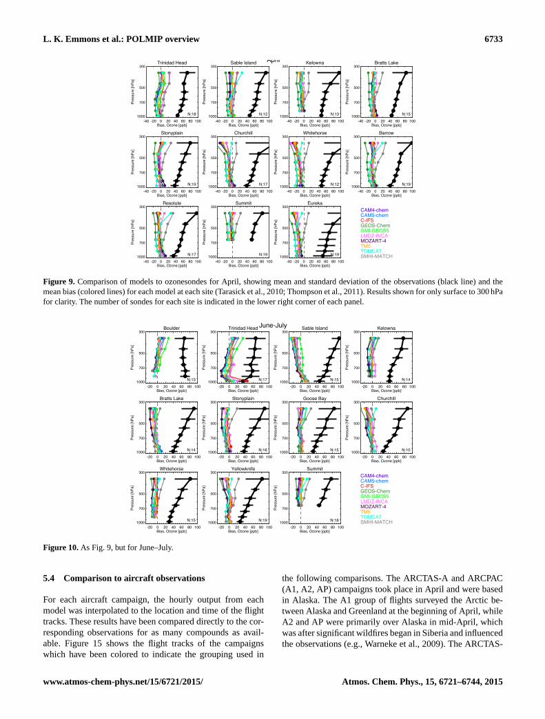
In April, the models generally underestimate the observed

ozone throughout the troposphere (negative bias). One con-

sistent exception is SMHI-MATCH, which is higher than ob-

served in the middle and upper troposphere, perhaps indicat-

ing that this model has too-strong transport of ozone from the

stratosphere. At all sites, GEOS-Chem has the lowest ozone

values at all altitudes above the boundary layer. TOMCAT

also has among the largest negative bias in the lower and mid-

troposphere, but is higher than most of the models at 300 hPa.

All the other models have a fairly uniform (across altitude

and sites) negative bias of about 5–10 ppb. The models have

slightly lower biases in June–July on average. At Kelowna


http://croc.gsfc.nasa.gov/arcions


and Goose Bay, the model biases fall within ±10 ppb; how-

ever, at several other sites (e.g., Churchill Lake and Bratt’s

Lake), the model mean biases are as much as 20 ppb be-

low the observations. These comparisons are consistent with

the ozone evaluation using aircraft observations presented by

Monks et al. (2014).

5.2 Surface network ethane and propane

The NOAA Global Monitoring Division/INSTAAR net-

work of surface sites provides weekly observations of light

NMHCs around the globe (Helmig et al., 2009). The model

results for ethane and propane are compared to the data over

a range of northern mid- to high latitudes in Fig. 11. Monthly

mean model output is used and the nearest grid point (lon-

gitude, latitude, altitude) selected for each site. All models

(except GEOS-Chem, which used higher ethane emissions

and has lower OH concentrations) significantly underesti-

mate the winter–spring observations, indicating the POLMIP

emissions are much too low for both C2H6 and C3H8, con-

sistent with the conclusion that CO emissions are too low (as

discussed in Sect. 5.4 and in Monks et al., 2014).

5.3 Evaluation of NO2

Satellite observations of NO2 have been used to evaluate the

individual model distributions of NO2 across the Northern

Hemisphere, as well as to evaluate the NOx emissions used

for all the models. Each model was compared to OMI (Ozone

Monitoring Instrument) DOMINO-v2 NO2 tropospheric col-

umn densities (Boersma et al., 2011), matching the times

of overpasses for each day and filtering out the pixels with

satellite-observed radiance fraction originating from clouds

greater than 50 %. In order to make a quantitative comparison

between model results and satellite retrievals (of any kind),

the sensitivity of the retrievals to the true atmospheric pro-

file must be taken into account. This is done by transforming

each model profile with the corresponding retrieval averag-

ing kernel and a priori information (e.g., Eskes and Boersma,

2003), hence making the evaluation independent of the a pri-

ori NO2 profiles used in DOMINO-v2. The transformation

of the model profiles with the averaging kernels gives model

levels in the free troposphere relatively greater weight in the

column calculation. For instance, depending on the surface

albedo the sensitivity to the upper free troposphere compared

to the surface layer may increase by roughly a factor of 3 (Es-

kes and Boersma, 2003). This means that errors in the shape

of the NO2 profile can contribute to biases in the total col-

umn.

The statistics of the biases between the model results and

the OMI NO2 tropospheric columns are used to evaluate the

NOx emissions inventory used in this study. Figure 12 shows

the NO2 tropospheric column from OMI for 18 June–15 July

(the period that hourly model output was provided) and the

median of the model biases for that period. The models gen-

ARCIONS Ozonesonde Locations

barrow

boulder

brattslake

churchill

egbert

eureka

goosebay

kelowna

narragansett

resolute

sableis

stonyplain

summit

trinidadhead

whitehorse

yarmouth

yellowknife

SpringSummer

Figure 8. Location of ARCIONS ozonesonde sites used in April

and June–July 2008 in coordination with ARCTAS.

erally underestimate NO2 over continental regions with high

levels of anthropogenic pollution (e.g., California, northeast-

ern United States, Europe, China); however, a few models

overestimate NO2 over North America (not shown). All mod-

els overestimate NO2 over northeast Asia, in the region of

fires (quantified below). OMI NO2 retrievals have low signal

to noise ratios over oceans and continental regions with low

pollutant levels; therefore, conclusions should not be drawn

by the model comparisons for those regions.

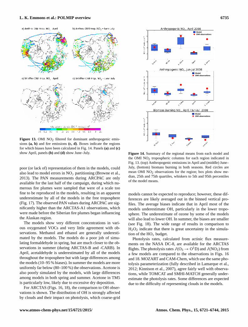
In Fig. 13 the OMI tropospheric columns are screened on

a daily basis for pixels where at least 90 % of the total NOxemissions, based on the emissions inventory, originate from

anthropogenic or biomass burning emissions, respectively.

Only pixels with significant emission levels are shown. In

this way, dominating source regions that are either primarily

anthropogenic or biomass burning can be identified. Boxes

are drawn around the highest concentrations in Fig. 13, and

the regional mean for each model, along with the mean ob-

served columns, are summarized in Fig. 14. The model re-

sults are lower than the observations for most of the an-

thropogenic region comparisons. For instance, NO2 columns

over South Korea are considerably underestimated. Also, the

inter-quartile range is relatively large for the Europe and east-

ern China regions indicating a large uncertainty introduced

by the models. Since all models used the same NO emis-

sions, the large variation among models (as seen in Fig. 14)

indicates differences in the chemistry and transport processes

affecting NO and NO2. The large region of biomass burn-

ing in western Asia (April) is well captured, but over eastern

Asia the models are typically too high. Also, the NO2 from

Siberian fires in July is greatly overestimated. The NO2 col-

umn amounts are much lower for the fires in Canada than in

Asia, but the models also overestimate the concentrations of

this region, suggesting the NOx emission factor is too high

for forests in the FINN emissions.



Trinidad Head

-40 -20 0 20 40 60 80 100Bias, Ozone [ppb]

1000

Pres

sure

[hPa

]

300

500

700

N:18

Sable Island

-40 -20 0 20 40 60 80 100Bias, Ozone [ppb]

1000

Pres

sure

[hPa

]

300

500

700

N:12

Kelowna

-40 -20 0 20 40 60 80 100Bias, Ozone [ppb]

1000

Pres

sure

[hPa

]

300

500

700

N:13

Bratts Lake

-40 -20 0 20 40 60 80 100Bias, Ozone [ppb]

1000

Pres

sure

[hPa

]

300

500

700

N:15

Stonyplain

-40 -20 0 20 40 60 80 100Bias, Ozone [ppb]

1000

Pres

sure

[hPa

]300

500

700

N:19

Churchill

-40 -20 0 20 40 60 80 100Bias, Ozone [ppb]

1000

Pres

sure

[hPa

]

300

500

700

N:17

Whitehorse

-40 -20 0 20 40 60 80 100Bias, Ozone [ppb]

1000

Pres

sure

[hPa

]

300

500

700

N:12

Barrow

-40 -20 0 20 40 60 80 100Bias, Ozone [ppb]

1000

Pres

sure

[hPa

]

300

500

700

N:19

Resolute

-40 -20 0 20 40 60 80 100Bias, Ozone [ppb]

1000

Pres

sure

[hPa

]

300

500

700

N:17

Summit

-40 -20 0 20 40 60 80 100Bias, Ozone [ppb]

1000

Pres

sure

[hPa

]300

500

700

N:19

Eureka

-40 -20 0 20 40 60 80 100Bias, Ozone [ppb]

1000

Pres

sure

[hPa

]

300

500

700

N:19

April


Figure 9. Comparison of models to ozonesondes for April, showing mean and standard deviation of the observations (black line) and the

mean bias (colored lines) for each model at each site (Tarasick et al., 2010; Thompson et al., 2011). Results shown for only surface to 300 hPa

for clarity. The number of sondes for each site is indicated in the lower right corner of each panel.

Boulder

-20 0 20 40 60 80 100Bias, Ozone [ppb]

1000

Pres

sure

[hPa

]

300

500

700

N:13

Trinidad Head

-20 0 20 40 60 80 100Bias, Ozone [ppb]

1000

Pres

sure

[hPa

]

300

500

700

N:17

Sable Island

-20 0 20 40 60 80 100Bias, Ozone [ppb]

1000

Pres

sure

[hPa

]

300

500

700

N:15

Kelowna

-20 0 20 40 60 80 100Bias, Ozone [ppb]

1000

Pres

sure

[hPa

]

300

500

700

N:14

Bratts Lake

-20 0 20 40 60 80 100Bias, Ozone [ppb]

1000

Pres

sure

[hPa

]

300

500

700

N:14

Stonyplain

-20 0 20 40 60 80 100Bias, Ozone [ppb]

1000

Pres

sure

[hPa

]

300

500

700

N:16

Goose Bay

-20 0 20 40 60 80 100Bias, Ozone [ppb]

1000

Pres

sure

[hPa

]

300

500

700

N:15

Churchill

-20 0 20 40 60 80 100Bias, Ozone [ppb]

1000

Pres

sure

[hPa

]

300

500

700

N:10

Whitehorse

-20 0 20 40 60 80 100Bias, Ozone [ppb]

1000

Pres

sure

[hPa

]

300

500

700

N:15

Yellowknife

-20 0 20 40 60 80 100Bias, Ozone [ppb]

1000

Pres

sure

[hPa

]

300

500

700

N:19

Summit

-20 0 20 40 60 80 100Bias, Ozone [ppb]

1000

Pres

sure

[hPa

]

300

500

700

N:18

June-July


Figure 10. As Fig. 9, but for June–July.

5.4 Comparison to aircraft observations

For each aircraft campaign, the hourly output from each

model was interpolated to the location and time of the flight

tracks. These results have been compared directly to the cor-

responding observations for as many compounds as avail-

able. Figure 15 shows the flight tracks of the campaigns

which have been colored to indicate the grouping used in

the following comparisons. The ARCTAS-A and ARCPAC

(A1, A2, AP) campaigns took place in April and were based

in Alaska. The A1 group of flights surveyed the Arctic be-

tween Alaska and Greenland at the beginning of April, while

A2 and AP were primarily over Alaska in mid-April, which

was after significant wildfires began in Siberia and influenced

the observations (e.g., Warneke et al., 2009). The ARCTAS-



ALT (82N, 297E)

Feb Apr Jun Aug Oct Dec0

500

1000

1500

2000

2500

3000

C2H6

[ppt

v]

SUM (72N, 321E)


500

1000

1500

2000

2500

3000

C2H6

[ppt

v]

BRW (71N, 203E)


1000

2000

3000

4000

C2H6

[ppt

v]

MHD (53N, 350E)


1000

2000

3000

4000

C2H6

[ppt

v]

SHM (52N, 185E)


500

1000

1500

2000

2500

C2H6

[ppt

v]

LEF (45N, 269E)


1000

2000

3000

4000

C2H6

[ppt

v]

ALT (82N, 297E)


200

400

600

800

1000

12001400

C3H8

[ppt

v]

SUM (72N, 321E)


500

1000

1500

C3H8

[ppt

v]

BRW (71N, 203E)


500

1000

1500

2000

C3H8

[ppt

v]

MHD (53N, 350E)


200

400

600

800

1000

12001400

C3H8

[ppt

v]

SHM (52N, 185E)


200

400

600

800

1000

1200

C3H8

[ppt

v]

LEF (45N, 269E)


500

1000

1500

2000

2500

3000

C3H8

[ppt

v]

CAM4-chemCAM5-chemC-IFSGEOS-ChemGMI-GEOS5LMDZ-INCAMOZART-4TM5TOMCAT

Figure 11. Ethane (top six panels) and propane (lower six panels) at

several Northern Hemisphere NOAA GMD network sites. Monthly

mean model output (colored lines) is plotted with 2008 weekly ob-

servations (black circles). Station codes: ALT: Alert, Canada; SUM:

Summit, Greenland; BRW: Barrow, Alaska; MHD: Mace Head, Ire-

land; SHM: Shemya, Alaska; LEF: Wisconsin.

CARB flights focused on characterizing urban and agricul-

tural emissions in California, but also sampled the wildfire

emissions present in the state. ARCTAS-B, based in central

Canada, sampled fresh and aged fire emissions over Canada

and into the Arctic. The POLARCAT-France and GRACE

experiments, based in southern Greenland, sampled down-

wind of anthropogenic and fire emissions regions and in-

cluded observations of air masses from North America, Asia,

and Europe.

Figures 16, 17 and 18 show vertical profiles of the obser-

vations with model results for the flights during ARCTAS-

A1, ARCPAC and ARCTAS-B, respectively. For these plots

the observations and the model results along the flight tracks

were treated in the same way: each group of flights was

binned according to altitude and the median value of each

1 km bin has been plotted. The thick error bars represent the

measurement uncertainty (determined by applying the frac-

tional uncertainty reported in each measurement data file to

the median binned value), while the thinner horizontal lines

Figure 12. (a) OMI tropospheric column NO2 and (b) median of

the model biases, both for 18 June–15 July.

show the variation (25th–75th percentiles) in the observa-

tions over the flights. In general the measurement uncertainty

is much less than the atmospheric variability; however for

ARCPAC, several measurements have relatively large uncer-

tainties (such as SO2, NO2 and HNO3).

In addition, the difference between each model and the ob-

servations was determined for each data point along the flight

tracks and then an average bias was determined for the alti-

tude range 3–7 km, as shown in Fig. 19. In the cases where a

compound was measured by more than one instrument, the

differences between the model and each observation were

averaged over all the measurement techniques. The uncer-

tainties shown in Figs. 16–18 need to be kept in mind when

considering the biases shown in Fig. 19.

Several models, but not all, underpredict ozone in spring

by more than 10 %, consistent with the ozonesonde compari-

son shown in Fig. 9. All models (except GEOS-chem) under-

predict CO and hydrocarbons in spring and summer, likely

indicating that the emissions used for POLMIP are too low.

NO and NO2 are generally underestimated in spring, with

NO2 biases ranging from 20 to 90 % too low. In summer, all

of the models match well the NO and NO2 observations in

the mid-troposphere, but NO2 is generally overestimated in

the boundary layer (ARCTAS-B; Fig. 18), consistent with the

OMI NO2 comparisons for the Canada fire regions (Fig. 14).

NOy partitioning between PAN and HNO3 is vastly dif-

ferent among the models (see Arnold et al., 2014). Many

models significantly overestimate HNO3 (by a factor of 10

in some cases), which could be primarily due to differences

in washout and missing loss processes. A new version of

LMDz-INCA includes the uptake of nitric acid on sea salt

and dust, accounting for 25 % of the total sink of nitric acid

(Hauglustaine et al., 2014). GMI includes otherwise unac-

counted for nitrogen species in HNO3, partially explaining

its overestimate. The simulated PAN values also vary signif-

icantly across models, which may be due to the differences

in PAN precursors (NOx and acetaldehyde) at anthropogenic

and fire source regions. Alkyl nitrates were found to be a sig-

nificant contribution to the NOy budget of the ARCTAS ob-

servations, particularly in low-NOx environments, and the



Figure 13. OMI NO2 filtered for dominant anthropogenic emis-

sions (a, b) and fire emissions (c, d). Boxes indicate the regions

for which biases have been calculated in Fig. 14. Panels (a) and (c)

show April, panels (b) and (d) show June–July.

poor (or lack of) representation of them in the models, could

also lead to model errors in NOy partitioning (Browne et al.,

2013). The PAN measurements during ARCPAC are only

available for the last half of the campaign, during which nu-

merous fire plumes were sampled that were of a scale too

fine to be reproduced in the models, resulting in an apparent

underestimate by all of the models in the free troposphere

(Fig. 17). The observed PAN values during ARCPAC are sig-

nificantly higher than the ARCTAS-A1 observations, which

were made before the Siberian fire plumes began influencing

the Alaskan region.

The models show very different concentrations in vari-

ous oxygenated VOCs and very little agreement with ob-

servations. Methanol and ethanol are generally underesti-

mated by the models. The models do a poor job of simu-

lating formaldehyde in spring, but are much closer to the ob-

servations in summer (during ARCTAS-B and -CARB). In

April, acetaldehyde is underestimated by all of the models

throughout the troposphere but with large differences among

the models (10–95 % biases). In summer the models are more

uniformly far below (80–100 %) the observations. Acetone is

also poorly simulated by the models, with large differences

among models in both spring and summer. Acetone in TM5

is particularly low, likely due to excessive dry deposition.

For ARCTAS (Figs. 16, 18), the comparison to OH obser-

vations is shown. The distribution of OH is strongly affected

by clouds and their impact on photolysis, which coarse-grid

Model&OMI&observa.ons&



Figure 14. Summary of the regional means from each model and

the OMI NO2 tropospheric columns for each region indicated in

Fig. 13. (top) Anthropogenic emissions in April and (middle) June–

July, (bottom) biomass burning in both seasons. Red circles are

mean OMI NO2 observations for the region; box plots show me-

dian, 25th and 75th quartiles, whiskers to 5th and 95th percentiles

of the model means.

models cannot be expected to reproduce; however, these dif-

ferences are likely averaged out in the binned vertical pro-

files. The average biases indicate that in April most of the

models underestimate OH, particularly in the lower tropo-

sphere. The underestimate of ozone by some of the models

will also lead to lower OH. In summer, the biases are smaller

(see Fig. 18). The wide range of results in comparison to

H2O2 indicate that there is great uncertainty in the simula-

tion of the HOx budget.

Photolysis rates, calculated from actinic flux measure-

ments on the NASA DC-8, are available for the ARCTAS

flights. The photolysis rates J (O3→ O1D) and J (NO2) from

a few models are compared to the observations in Figs. 16

and 18. MOZART and CAM-Chem, which use the same pho-

tolysis parameterization (fully described in Lamarque et al.,

2012; Kinnison et al., 2007), agree fairly well with observa-

tions, while TOMCAT and SMHI-MATCH generally under-

estimate the photolysis rates. Some differences are expected

due to the difficulty of representing clouds in the models.



ARCTAS-A1ARCTAS-A2ARCPACARCTAS-CARBARCTAS-BGRACEPOLARCAT-France

Figure 15. Location of aircraft flight tracks. ARCTAS-A1: 4–

9 April; ARCTAS-A2: 12–17 April; ARCPAC: 11–21 April;

ARCTAS-CARB: 18–24 June; ARCTAS-B: 29 June–10 July;

GRACE: 30 June–18 July; POLARCAT-France: 30 June–14 July.

6 Enhancement ratios of VOCs in fires

The measurements of numerous compounds and the frequent

sampling of air masses influenced by wildfires by the DC-

8 aircraft during ARCTAS allowed for a derivation of en-

hancement factors of VOCs relative to CO for several sets

of fires, as cataloged and summarized by Hornbrook et al.

(2011). In that analysis, Hornbrook et al. (2011) used a va-

riety of parameters to identify fire-influenced air masses,

their origin, age, including acetonitrile and hydrogen cyanide

(CH3CN and HCN, which have primarily biomass burn-

ing sources), back trajectories from the aircraft flight tracks,

and NMHC ratios (to determine photochemical age). Dur-

ing ARCTAS-B, numerous observations were made of fresh

plumes from the fires burning in Saskatchewan, providing

good statistics of the enhancement ratios. Since the photo-

chemical age of these sampled plumes was generally less

than 2 days, the error introduced due to chemical processing

of the plumes is much less than for the older plumes from

Asia, for example. The sampling of fresh plumes from the

fires in Saskatchewan, with little influence of local anthro-

pogenic sources, makes this a good period and location for

the evaluation of fire emissions in the models.

Due to the coarse resolution of the models, along with the

uncertainties in location, vertical distribution and strength of

the sources, it is not expected that the models will capture

the magnitude or exact location of plumes that were sam-

pled by the aircraft. Therefore, instead of using the model

results interpolated to the flight tracks, all of the grid points

with CO mixing ratios greater than 150 ppb within the re-

gion of the fires (54–58◦ N, 252–258◦ E, model levels be-

tween the surface and 850 hPa) were used from the hourly

output from each model. This model output was used to de-

rive enhancement ratios of VOCs relative to CO, comparable

to those derived by Hornbrook et al. (2011) (given in their

Table 2 and Fig. 7). Figure 20 shows the enhancement ratios

derived from the aircraft measurements, giving the mean and

standard deviation of all observed Saskatchewan fire plumes.

Also shown in Fig. 20 are the emission factors (EF) deter-

mined from the emissions inventory used by the models, av-

eraged over 28 June–5 July and 54–58◦ N, 252–258◦ E. For

each model, the enhancement ratio was determined as the

slope of a linear fit to the correlation of each VOC to CO.

For the VOCs with direct emissions and little or no sec-

ondary production (ethane, propane, methanol, ethanol), the

VOC /CO ratios of the model mixing ratios are very close

to the emission factors of the inventory used by the models.

This indicates the chemical processing in the vicinity of the

fires is slow enough that the observations are a good indica-

tor of the actual fire emission factors. This also means the

model ratios can be quantitatively compared to the observa-

tions. Thus, we can conclude for the Saskatchewan fires that

the fire emission factors used are too high for ethane, too

low for propane, about right for methanol and much too low

for ethanol. However, the compounds that have significant

chemical production in addition to emissions (i.e., formalde-

hyde, acetaldehyde and acetone) have very different mixing

VOC /CO ratios from the emission ratios. The model en-

hancement ratios of CH2O and CH3CHO are significantly

higher than the inventory emission factors due to chemical

production, but they agree well with the observations. The

model ratios for acetone, however, are lower than the obser-

vations but not very different from the emission factor, im-

plying the emission factors are too low.

7 Conclusions

Eleven global or regional chemistry models participated in

the POLARCAT Model Intercomparison Project (POLMIP),

allowing for an assessment of our current understanding of

the chemical and transport processes affecting the distribu-

tions of ozone and its precursors in the Arctic. To limit

the differences among models, a standard emissions inven-

tory was used. All of the models were driven, to at least

some degree, by observed meteorology (GEOS-5, NCEP

or ECMWF) and therefore represented the dynamics of the

study year (2008).

While the extensive suite of aircraft observations in 2008

at high northern latitudes is extremely valuable for evalu-

ating the models, they cannot uniquely identify the source

of emissions errors, as the Arctic is influenced by many

sources at lower latitudes. However, several conclusions can

be drawn about the emissions inventory used in this study.

Based on the comparisons to aircraft observations and the

NOAA surface network data, emissions of CO, ethane and

propane are clearly too low. The comparisons to satellite re-

trievals of OMI NO2 show a few regions of consistent model

errors that indicate that anthropogenic NOx emissions are

underestimated in East Asia, while fire emissions are over-

estimated in Siberia. Large differences are seen among the

model NO2 tropospheric columns over Europe and China,



O3

0 50 100 150[ppbv]

02468

1012

Altit

ude

[km

]

CO

0 50 100 150 200 250[ppbv]

02468

1012

Altit

ude

[km

]

C2H6

0 1000 2000 3000[pptv]

02468

1012

Altit

ude

[km

]

C3H8

0 200 400 600 800 1000[pptv]

02468

1012

Altit

ude

[km

]

NO

0 20 40 60 80 100[pptv]

02468

1012

Altit

ude

[km

]

NO2

0 20 40 60[pptv]

02468

1012

Altit

ude

[km

]

PAN

0 200 400 600 800[pptv]

02468

1012

Altit

ude

[km

]

HNO3

0 100 200 300 400[pptv]

02468

1012

Altit

ude

[km

]

SO2

0 100 200 300[pptv]

02468

1012

Altit

ude

[km

]

H2O2

0 200 400 600 800[pptv]

02468

1012

Altit

ude

[km

]

CH3OH

0 200 400 600 800 1000[pptv]

02468

1012

Altit

ude

[km

]

C2H5OH

0 20 40 60 80 100[pptv]

02468

1012

Altit

ude

[km

]

CH2O

0 50 100 150 200 250[pptv]

02468

1012

Altit

ude

[km

]

CH3CHO

0 50 100 150 200[pptv]

02468

1012

Altit

ude

[km

]

CH3COCH3

0 500 1000 1500[pptv]

02468

1012

Altit

ude

[km

]

OH

0.00 0.05 0.10 0.15 0.20[pptv]

02468

1012

Altit

ude

[km

]

J(O1D)

0 5 10 15[10-6 * 1/s]

02468

1012

Altit

ude

[km

]

J(NO2)

0 5 10 15 20[10-3 * 1/s]

02468

1012

Altit

ude

[km

]

ARCTAS-A1

CAM4-chemCAM5-chemC-IFSGEOS-ChemGMI-GEOS5LMDZ-INCA

MOZART-4TM5TOMCATSMHI-MATCH

Figure 16. Comparison of model results interpolated to flight tracks of observations during the first four DC-8 flights of ARCTAS-A. Each

profile is the median of 1 km altitude bins. Medians of observations in each 1 km altitude bin are shown as black circles and crosses (if

a second measurement exists for a given parameter). Thick error bars represent the measurement uncertainty; thin error bars span inter-

quartile range of all observations.

O3

0 20 40 60 80 100[ppbv]

0

2

4

6

8

Altit

ude

[km

]

CO

0 50 100 150 200 250[ppbv]

0

2

4

6

8

Altit

ude

[km

]

C3H8

0 200 400 600 800[pptv]

0

2

4

6

8

Altit

ude

[km

]

SO2

0 50 100 150 200 250 300[pptv]

0

2

4

6

8

Altit

ude

[km

]

NO

0 10 20 30 40[pptv]

0

2

4

6

8

Altit

ude

[km

]

NO2

0 20 40 60 80 100[pptv]

0

2

4

6

8

Altit

ude

[km

]

PAN

0 500 1000 1500[pptv]

0

2

4

6

8

Altit

ude

[km

]

HNO3

0 100 200 300 400[pptv]

0

2

4

6

8

Altit

ude

[km

]

CH3OH

0 500 1000 1500 2000[pptv]

0

2

4

6

8

Altit

ude

[km

]

CH3COCH3

0 500 1000 1500[pptv]

0

2

4

6

8

Altit

ude

[km

]

ARCPAC


MOZART-4TM5TOMCATSMHI-MATCH

Figure 17. As Fig. 16, for ARCPAC NOAA P3 observations.



O3

0 50 100 150[ppbv]

02468

1012

Altit

ude

[km

]

CO

0 50 100 150 200 250[ppbv]

02468

1012

Altit

ude

[km

]

C2H6

0 500 1000 1500 2000[pptv]

02468

1012

Altit

ude

[km

]

C3H8

0 100 200 300 400 500[pptv]

02468

1012

Altit

ude

[km

]

NO

0 20 40 60 80 100[pptv]

02468

1012

Altit

ude

[km

]

NO2

0 20 40 60[pptv]

02468

1012

Altit

ude

[km

]PAN

0 200 400 600 800[pptv]

02468

1012

Altit

ude

[km

]

HNO3

0 200 400 600 800[pptv]

02468

1012

Altit

ude

[km

]

SO2

0 100 200 300 400[pptv]

02468

1012

Altit

ude

[km

]

H2O2

0 1000 2000 3000[pptv]

02468

1012

Altit

ude

[km

]

CH3OH

0 2000 4000 6000[pptv]

02468

1012

Altit

ude

[km

]

C2H5OH

0 100 200 300 400[pptv]

02468

1012

Altit

ude

[km

]CH2O

0 1000 2000 3000[pptv]

02468

1012

Altit

ude

[km

]

CH3CHO

0 200 400 600 800[pptv]

02468

1012

Altit

ude

[km

]

CH3COCH3

0 1000 2000 3000[pptv]

02468

1012

Altit

ude

[km

]

OH

0.000.050.100.150.200.250.30[pptv]

02468

1012

Altit

ude

[km

]

J(O1D)

0 10 20 30 40[10-6 * 1/s]

02468

1012

Altit

ude

[km

]

J(NO2)

0 5 10 15 20[10-3 * 1/s]

02468

1012

Altit

ude

[km

]

ARCTAS-B


MOZART-4TM5TOMCATSMHI-MATCHWRF-Chem/100kmWRF-Chem/50km

Figure 18. As Fig. 16, for ARCTAS-B DC-8 observations.

O3

A1 A2 AP C B -40-30-20-10

0102030

CO

A1 A2 AP C B -40

-30

-20

-10

0

10C2H6

A1 A2 AP C B -100

-50

0

50

100C3H8

A1 A2 AP C B -100

-80

-60

-40

-20

0NO

A1 A2 AP C B -100

-50

0

50

100

150

NO2

A1 A2 AP C B -100-80-60-40-20

02040

PAN

A1 A2 AP C B -100

-50

0

50

100

150HNO3

A1 A2 AP C B -500

0

500

1000

1500H2O2

A1 A2 AP C B -100-80-60-40-20

02040

CH2O

A1 A2 AP C B -100-80

-60

-40

-20

020

CH3CHO

A1 A2 AP C B -100

-80

-60

-40

-20

0Methanol

A1 A2 AP C B -100-80-60-40-20

02040

Acetone

A1 A2 AP C B -100-80

-60

-40

-20

020

SO2

A1 A2 AP C B -100-80-60-40-20

02040

Mod

el B

ias

(%)

Campaign

CAM4-chemCAM5-chemC-IFSGEOS-ChemGMI-GEOS5LMDZ-INCAMOZART-4TM5TOMCATSMHI-MATCHWRF-Chem/100kmWRF-Chem/50km

Figure 19. Mean bias (%) between models and aircraft observations, averaged over 3–7 km. Bias for multiple measurements of a single

compound are also averaged over each campaign, which are A1: ARCTAS-A 4–9 April; A2: ARCTAS-A 12–17 April; AP: ARCPAC

11–21 April; C: ARCTAS-CARB 18–24 June; and B: ARCTAS-B 29 June–10 July.

thus limiting the conclusions that can be drawn regarding the

accuracy of the emissions inventory. The large range in mod-

eled NO2 (where NOx emissions were the same) also indi-

cates that model chemistry and boundary layer parameteri-

zations can significantly impact NOx chemistry. More accu-

rate emissions inventories might greatly improve many of the

model deficiencies identified in this study. Emissions inven-

tories modified based on inverse modeling results, as well as



C2H6

Obs EF Models

0

2

4

6

8

10

12

14

C2H6

/CO

[ppt

/ppb

]

C3H8

Obs EF Models

0.0

0.5

1.0

1.5

2.0

2.5

C3H8

/CO

[ppt

/ppb

]

CH3OH

Obs EF Models

0

5

10

15

20

25

30

CH3O

H/CO

[ppt

/ppb

]

C2H5OH

Obs EF Models

0.0

0.1

0.2

0.3

0.4

0.5

C2H5

OH/

CO [p

pt/p

pb]

CH2O

Obs EF Models

0

5

10

15

20

CH2O

/CO

[ppt

/ppb

]

CH3CHO

Obs EF Models

0

2

4

6

8

10

CH3C

HO/C

O [p

pt/p

pb]

CH3COCH3

Obs EF Models

0

2

4

6

8

10

CH3C

OCH

3/CO

[ppt

/ppb

]Obs. enhancement ratioEmission factorCAM4-chemCAM5-chemC-IFSGEOS-ChemGMI-GEOS5LMDZ-INCAMOZART-4TM5TOMCAT

SaskatchewanJun 28-Jul 5

Figure 20. Correlations of VOCs to CO for the POLMIP models,

compared to those derived from the DC-8 observations for the fires

in Saskatchewan. The filled circle shows the enhancement ratio de-

rived from DC-8 observations (Hornbrook et al., 2011). The asterisk

shows the EF of the model emissions. The colored diamonds are the

enhancement ratios determined for each model.

results of this study, will be used in future work as one step

in improving model simulations of Arctic atmospheric com-

position.

The simultaneous evaluation of the models with observa-

tions of reactive nitrogen species and VOCs has illustrated

that large differences exist in the model chemical mecha-

nisms, especially in their representation of VOCs and their

oxidation. Most of the models showed a negative bias in

comparison to ozone observations from sondes and aircraft,

with a slightly larger difference in April than in summer. The

models frequently underestimated ozone in the free tropo-

sphere by 10–20 ppb in the comparison with ozonesondes.

In addition, 10–30 % negative model biases were seen in

comparison to the mid-troposphere aircraft ozone measure-

ments. Comparisons for ozone precursors such as NOx , PAN,

and VOCs show much greater biases and differences among

models. It appears numerous factors are the causes of these

model differences. The differences among model photolysis

rates and cloud distributions indicate some of the possible

causes for differences in modeled OH, which leads to dif-

ferences in numerous species and ozone production and loss

rates.

Some differences among the simulated results are likely

due to different physical parameterizations such as convec-

tion, boundary layer mixing and ventilation, wet and dry de-

position. Additional model diagnostics are required to bet-

ter understand the differences among models. For example,

comparison of the wet deposition rates and fluxes of a num-

ber of compounds could be informative in understanding the

budgets of NOy , HOx and VOCs.

Evaluation of chemical transport models with numerous

simultaneous observations, such as those of the POLARCAT

aircraft experiments, can assist in a critical assessment of

ozone simulations and identify model components in need

of improvement. Model representation of the oxidation of

VOCs and the NOy budget can have a significant impact

on ozone distributions. Future chemical model comparisons

should consider evaluation of VOCs and reactive nitrogen

species as an important component of the evaluation of ozone

simulations.

Acknowledgements. The numerous individuals who provided ob-

servations used in this study are gratefully acknowledged, in-

cluding William H. Brune, Jingqiu Mao, Xinrong Ren, and

David Shelow of Pennsylvania State University for the ARCTAS

DC8 LIF OH measurements; Paul Wennberg and John Crounse

of California Institute of Technology for the ARCTAS DC8

CIT-CIMS data (supported by NASA award NNX08AD29G);

Steve Montzka of NOAA/ESRL/GMD for NOAA P3 flask samples

of propane during ARCPAC; Joost de Gouw of NOAA/ESRL/CSD

for ARCPAC PTRMS VOC observations; and John Holloway of

NOAA/ESRL/CSD for ARCPAC CO and SO2 (UV fluorescence)

measurements.

The GEOS-5 data used with CAM-chem in this study have been

provided by the Global Modeling and Assimilation Office (GMAO)

at NASA Goddard Space Flight Center. We acknowledge the free

use of tropospheric NO2 column data from the OMI sensor from

www.temis.nl. French co-authors acknowledge funding from the

French Agence National de Recherche (ANR) CLIMSLIP project

and CNRS-LEFE. POLARCAT-France was supported by ANR,

CNRS-LEFE and CNES. This work was performed in part using

HPC resources from GENCI-IDRIS (grant 2014-017141). V. Huij-

nen acknowledges funding from the European Commission under

the Seventh Framework Programme (contract number 218793).

Contributions by SMHI were funded by the Swedish Environmen-

tal Protection Agency under contract NV-09414-12 and through

the Swedish Climate and Clean Air research program, SCAC.

A. Wisthaler acknowledges support from BMVIT-FFG/ALR.

ARCPAC was supported in part by the NOAA Climate and Health

of the Atmosphere programs. J. Mao acknowledges the NOAA Cli-

mate Program Office’s grant NA13OAR4310071. L. K. Emmons

acknowledges support from the National Aeronautics and Space

Administration under award no. NNX08AD22G issued through the

Science Mission Directorate, Tropospheric Composition Program.

The CESM project is supported by the National Science Foundation

and the Office of Science (BER) of the US Department of Energy.

The National Center for Atmospheric Research is funded by the

National Science Foundation.

Edited by: M. Schulz

References

Andersson, C., Langner, J., and Bergstrom, R.: Interannual variation

and trends in air pollution over Europe due to climate variability

during 1958–2001 simulated with a regional CTM coupled to

the ERA40 reanalysis, Tellus B, 59, 77–98, doi:10.1111/j.1600-

0889.2006.00196.x, 2007.


www.temis.nl

http://dx.doi.org/10.1111/j.1600-0889.2006.00196.x

http://dx.doi.org/10.1111/j.1600-0889.2006.00196.x


Arnold, S. R., Methven, J., Evans, M. J., Chipperfield, M. P.,

Lewis, A. C., Hopkins, J. R., McQuaid, J. B., Watson, N.,

Purvis, R. M., Lee, J. D., Atlas, E. L., Blake, D. R., and Rap-

penglueck, B.: Statistical inference of OH concentrations and air

mass dilution rates from successive observations of nonmethane

hydrocarbons in single air masses, J. Geophys. Res.-Atmos., 112,

D10S40, doi:10.1029/2006JD007594, 2007.

Arnold, S. R., Emmons, L. K., Monks, S. A., Law, K. S., Rid-

ley, D. A., Turquety, S., Tilmes, S., Thomas, J. L., Bouarar, I.,

Flemming, J., Huijnen, V., Mao, J., Duncan, B. N., Steenrod, S.,

Yoshida, Y., Langner, J., and Long, Y.: Biomass burning in-

fluence on high latitude tropospheric ozone and reactive nitro-

gen in summer 2008: a multi-model analysis based on POLMIP

simulations, Atmos. Chem. Phys. Discuss., 14, 24573–24621,

doi:10.5194/acpd-14-24573-2014, 2014.

Barrie, L. A.: Arctic air pollution: an overview of current

knowledge, Atmos. Environ., 20, 643–663, doi:10.1016/0004-

6981(86)90180-0, 1986.

Bey, I., Jacob, D. J., Yantosca, R. M., Logan, J. A., Field, B. D.,

Fiore, A. M., Li, Q., Liu, H. Y., Mickley, L. J., and

Schultz, M. G.: Global modeling of tropospheric chem-

istry with assimilated meteorology: model description and

evaluation, J. Geophys. Res.-Atmos., 106, 23073–23095,

doi:10.1029/2001JD000807, 2001.

Boersma, K. F., Eskes, H. J., Dirksen, R. J., van der A, R. J.,

Veefkind, J. P., Stammes, P., Huijnen, V., Kleipool, Q. L.,

Sneep, M., Claas, J., Leitão, J., Richter, A., Zhou, Y., and Brun-

ner, D.: An improved tropospheric NO2 column retrieval algo-

rithm for the Ozone Monitoring Instrument, Atmos. Meas. Tech.,

4, 1905–1928, doi:10.5194/amt-4-1905-2011, 2011.

Brock, C. A., Cozic, J., Bahreini, R., Froyd, K. D., Middle-

brook, A. M., McComiskey, A., Brioude, J., Cooper, O. R.,

Stohl, A., Aikin, K. C., de Gouw, J. A., Fahey, D. W., Fer-

rare, R. A., Gao, R.-S., Gore, W., Holloway, J. S., Hübler, G.,

Jefferson, A., Lack, D. A., Lance, S., Moore, R. H., Mur-

phy, D. M., Nenes, A., Novelli, P. C., Nowak, J. B., Ogren, J. A.,

Peischl, J., Pierce, R. B., Pilewskie, P., Quinn, P. K., Ryer-

son, T. B., Schmidt, K. S., Schwarz, J. P., Sodemann, H., Spack-

man, J. R., Stark, H., Thomson, D. S., Thornberry, T., Veres, P.,

Watts, L. A., Warneke, C., and Wollny, A. G.: Characteristics,

sources, and transport of aerosols measured in spring 2008 dur-

ing the aerosol, radiation, and cloud processes affecting Arc-

tic Climate (ARCPAC) Project, Atmos. Chem. Phys., 11, 2423–

2453, doi:10.5194/acp-11-2423-2011, 2011.

Browne, E. C., Min, K.-E., Wooldridge, P. J., Apel, E., Blake, D. R.,

Brune, W. H., Cantrell, C. A., Cubison, M. J., Diskin, G. S.,

Jimenez, J. L., Weinheimer, A. J., Wennberg, P. O., Wisthaler, A.,

and Cohen, R. C.: Observations of total RONO2 over the boreal

forest: NOx sinks and HNO3 sources, Atmos. Chem. Phys., 13,

4543–4562, doi:10.5194/acp-13-4543-2013, 2013.

Chin, M., Ginoux, P., Kinne, S., Torres, O., Holben, B., Duncan, B.,

Martin, R., Logan, J., Higurashi, A., and Nakajima, T.: Tro-

pospheric aerosol optical thickness from the GOCART model

and comparisons with satellite and Sun photometer measure-

ments, J. Atmos. Sciences, 59, 461–483, doi:10.1175/1520-

0469(2002)059<0461:TAOTFT>2.0.CO;2, 2002.

Chipperfield, M. P.: New version of the TOMCAT/SLIMCAT off-

line chemical transport model: intercomparison of stratospheric

tracer experiments, Q. J. Roy. Meteor. Soc., 132, 1179–1203,

doi:10.1256/qj.05.51, 2006.

DeCaria, A. J., Pickering, K. E., Stenchikov, G. L., and

Ott, L. E.: Lightning-generated NOx and its impact on tropo-

spheric ozone production: a three-dimensional modeling study

of a Stratosphere–Troposphere Experiment: Radiation, Aerosols

and Ozone (STERAO-A) thunderstorm, J. Geophys. Res.-

Atmos., 110, D14303, doi:10.1029/2004JD005556, 2005.

de Villiers, R. A., Ancellet, G., Pelon, J., Quennehen, B.,

Schwarzenboeck, A., Gayet, J. F., and Law, K. S.: Airborne mea-

surements of aerosol optical properties related to early spring

transport of mid-latitude sources into the Arctic, Atmos. Chem.

Phys., 10, 5011–5030, doi:10.5194/acp-10-5011-2010, 2010.

Duncan, B. N., Strahan, S. E., Yoshida, Y., Steenrod, S. D., and

Livesey, N.: Model study of the cross-tropopause transport of

biomass burning pollution, Atmos. Chem. Phys., 7, 3713–3736,

doi:10.5194/acp-7-3713-2007, 2007.

Emmons, L. K., Walters, S., Hess, P. G., Lamarque, J.-F., Pfis-

ter, G. G., Fillmore, D., Granier, C., Guenther, A., Kinnison, D.,

Laepple, T., Orlando, J., Tie, X., Tyndall, G., Wiedinmyer, C.,

Baughcum, S. L., and Kloster, S.: Description and evaluation of

the Model for Ozone and Related chemical Tracers, version 4

(MOZART-4), Geosci. Model Dev., 3, 43–67, doi:10.5194/gmd-

3-43-2010, 2010.

Engvall, A.-C., Krejci, R., Strom, J., Minikin, A., Treffeisen, R.,

Stohl, A., and Herber, A.: In-situ airborne observations of

the microphysical properties of the Arctic tropospheric aerosol

during late spring and summer, Tellus B, 60, 392–404,

doi:10.1111/j.1600-0889.2008.00348.x, 2008.

Eskes, H. J. and Boersma, K. F.: Averaging kernels for DOAS total-

column satellite retrievals, Atmos. Chem. Phys., 3, 1285–1291,

doi:10.5194/acp-3-1285-2003, 2003.

Fast, J. D., Gustafson, W. I., Easter, R. C., Zaveri, R. A.,

Barnard, J. C., Chapman, E. G., Grell, G. A., and Peck-

ham, S. E.: Evolution of ozone, particulates, and aerosol direct

radiative forcing in the vicinity of Houston using a fully coupled

meteorology-chemistry-aerosol model, J. Geophys. Res.-Atmos.,

111, D21305, doi:10.1029/2005JD006721, 2006.

Fisher, J. A., Jacob, D. J., Purdy, M. T., Kopacz, M., Le Sager, P.,

Carouge, C., Holmes, C. D., Yantosca, R. M., Batchelor, R. L.,

Strong, K., Diskin, G. S., Fuelberg, H. E., Holloway, J. S.,

Hyer, E. J., McMillan, W. W., Warner, J., Streets, D. G.,

Zhang, Q., Wang, Y., and Wu, S.: Source attribution and in-

terannual variability of Arctic pollution in spring constrained

by aircraft (ARCTAS, ARCPAC) and satellite (AIRS) observa-

tions of carbon monoxide, Atmos. Chem. Phys., 10, 977–996,

doi:10.5194/acp-10-977-2010, 2010.

Flemming, J., Huijnen, V., Arteta, J., Bechtold, P., Beljaars, A.,

Blechschmidt, A.-M., Diamantakis, M., Engelen, R. J., Gaudel,

A., Inness, A., Jones, L., Josse, B., Katragkou, E., Marecal,

V., Peuch, V.-H., Richter, A., Schultz, M. G., Stein, O., and

Tsikerdekis, A.: Tropospheric chemistry in the Integrated Fore-

casting System of ECMWF, Geosci. Model Dev., 8, 975–1003,

doi:10.5194/gmd-8-975-2015, 2015.

Folberth, G. A., Hauglustaine, D. A., Lathière, J., and Brocheton, F.:

Interactive chemistry in the Laboratoire de Météorologie Dy-

namique general circulation model: model description and im-

pact analysis of biogenic hydrocarbons on tropospheric chem-


http://dx.doi.org/10.1029/2006JD007594

http://dx.doi.org/10.5194/acpd-14-24573-2014

http://dx.doi.org/10.1016/0004-6981(86)90180-0

http://dx.doi.org/10.1016/0004-6981(86)90180-0

http://dx.doi.org/10.1029/2001JD000807

http://dx.doi.org/10.5194/amt-4-1905-2011

http://dx.doi.org/10.5194/acp-11-2423-2011


http://dx.doi.org/10.1175/1520-0469(2002)059<0461:TAOTFT>2.0.CO;2

http://dx.doi.org/10.1175/1520-0469(2002)059<0461:TAOTFT>2.0.CO;2

http://dx.doi.org/10.1256/qj.05.51

http://dx.doi.org/10.1029/2004JD005556



http://dx.doi.org/10.5194/gmd-3-43-2010


http://dx.doi.org/10.1111/j.1600-0889.2008.00348.x


http://dx.doi.org/10.1029/2005JD006721




istry, Atmos. Chem. Phys., 6, 2273–2319, doi:10.5194/acp-6-

2273-2006, 2006.

Freitas, S. R., Longo, K. M., Chatfield, R., Latham, D.,

Silva Dias, M. A. F., Andreae, M. O., Prins, E., Santos, J. C.,

Gielow, R., and Carvalho Jr., J. A.: Including the sub-grid

scale plume rise of vegetation fires in low resolution atmo-

spheric transport models, Atmos. Chem. Phys., 7, 3385–3398,

doi:10.5194/acp-7-3385-2007, 2007.

Granier, C., Lamarque, J., Mieville, A., Müller, J., Olivier, J.,

Orlando, J., Peters, J., Petron, G., Tyndall, G., and Wal-

lens, S.: POET, a database of surface emissions of ozone pre-

cursors, available at: http://www.pole-ether.fr/eccad (last access:

19 November 2014), 2005.

Granier, C., Bessagnet, B., Bond, T., D’Angiola, A., Denier van der

Gon, H., Frost, G. J., Heil, A., Kaiser, J. W., Kinne, S., Klimont,

Z., Kloster, S., Lamarque, J.-F., Liousse, C., Masui, T., Meleux,

F., Mieville, A., Ohara, T., Raut, J.-C., Riahi, K., Schultz, M. G.,

Smith, S. J., Thompson, A., van Aardenne, J., van der Werf,

G. R., and van Vuuren, D. P.: Evolution of anthropogenic and

biomass burning emissions of air pollutants at global and re-

gional scales during the 1980–2010 period, Climatic Change,

109, 163–190, doi:10/1007/s10584-011-0154-1, 2011.

Grell, G., Peckham, S., Schmitz, R., McKeen, S., Frost, G.,

Skamarock, W., and Eder, B.: Fully coupled “online” chem-

istry within the WRF model, Atmos. Environ., 39, 6957–6975,

doi:10.1016/j.atmosenv.2005.04.027, 2005.

Hauglustaine, D. A., Hourdin, F., Jourdain, L., Filiberti, M.-A.,

Walters, S., Lamarque, J.-F., and Holland, E. A.: Interactive

chemistry in the Laboratoire de Météorologie Dynamique gen-

eral circulation model: description and background tropospheric

chemistry evaluation, J. Geophys. Res.-Atmos., 109, D04314,

doi:10.1029/2003JD003957, 2004.

Hauglustaine, D. A., Balkanski, Y., and Schulz, M.: A global model

simulation of present and future nitrate aerosols and their direct

radiative forcing of climate, Atmos. Chem. Phys., 14, 11031–

11063, doi:10.5194/acp-14-11031-2014, 2014.

Helmig, D., Ganzeveld, L., Butler, T., and Oltmans, S. J.: The role of

ozone atmosphere-snow gas exchange on polar, boundary-layer

tropospheric ozone – a review and sensitivity analysis, Atmos.

Chem. Phys., 7, 15–30, doi:10.5194/acp-7-15-2007, 2007a.

Helmig, D., Oltmans, S., Morse, T., and Dibb, J.: What is causing

high ozone at Summit, Greenland, Atmos. Environ., 41, 5031–

5043, 2007b.

Helmig, D., Bottenheim, J., Galbally, I. E., Lewis, A., Milton, M.

J. T., Penkett, S., Plass-Duelmer, C., Reimann, S., Tans, P., and

Thiel, S.: Volatile organic compounds in the global atmosphere,

EOS T. Am. Geophys. Un., 90, 513–514, 2009.

Hornbrook, R. S., Blake, D. R., Diskin, G. S., Fried, A.,

Fuelberg, H. E., Meinardi, S., Mikoviny, T., Richter, D.,

Sachse, G. W., Vay, S. A., Walega, J., Weibring, P., Wein-

heimer, A. J., Wiedinmyer, C., Wisthaler, A., Hills, A.,

Riemer, D. D., and Apel, E. C.: Observations of nonmethane or-

ganic compounds during ARCTAS – Part 1: Biomass burning

emissions and plume enhancements, Atmos. Chem. Phys., 11,

11103–11130, doi:10.5194/acp-11-11103-2011, 2011.

Hourdin, F., Musat, I., Bony, S., Braconnot, P., Codron, F.,

Dufresne, J.-L., Fairhead, L., Filiberti, M.-A., Friedlingstein, P.,

Grandpeix, J.-Y., Krinner, G., LeVan, P., Li, Z.-X., and Lott, F.:

The LMDZ4 general circulation model: climate performance and

sensitivity to parametrized physics with emphasis on tropical

convection, Clim. Dynam., 27, 787–813, doi:10.1007/s00382-

006-0158-0, 2006.

Huang, M., Carmichael, G. R., Adhikary, B., Spak, S. N., Kulka-

rni, S., Cheng, Y. F., Wei, C., Tang, Y., Parrish, D. D.,

Oltmans, S. J., D’Allura, A., Kaduwela, A., Cai, C., Wein-

heimer, A. J., Wong, M., Pierce, R. B., Al-Saadi, J. A.,

Streets, D. G., and Zhang, Q.: Impacts of transported background

ozone on California air quality during the ARCTAS-CARB pe-

riod – a multi-scale modeling study, Atmos. Chem. Phys., 10,

6947–6968, doi:10.5194/acp-10-6947-2010, 2010.

Huijnen, V., Williams, J., van Weele, M., van Noije, T., Krol, M.,

Dentener, F., Segers, A., Houweling, S., Peters, W., de Laat, J.,

Boersma, F., Bergamaschi, P., van Velthoven, P., Le Sager, P., Es-

kes, H., Alkemade, F., Scheele, R., Nédélec, P., and Pätz, H.-W.:

The global chemistry transport model TM5: description and eval-

uation of the tropospheric chemistry version 3.0, Geosci. Model

Dev., 3, 445–473, doi:10.5194/gmd-3-445-2010, 2010.

Jacob, D. J., Crawford, J. H., Maring, H., Clarke, A. D., Dibb, J. E.,

Emmons, L. K., Ferrare, R. A., Hostetler, C. A., Russell, P. B.,

Singh, H. B., Thompson, A. M., Shaw, G. E., McCauley, E., Ped-

erson, J. R., and Fisher, J. A.: The Arctic Research of the Compo-

sition of the Troposphere from Aircraft and Satellites (ARCTAS)

mission: design, execution, and first results, Atmos. Chem. Phys.,

10, 5191–5212, doi:10.5194/acp-10-5191-2010, 2010.

Jourdain, L. and Hauglustaine, D.: The global distribution of light-

ning NOx simulated on-line in a general circulation model,

Phys. Chem. Earth Pt. C, 26, 585–591, doi:10.1016/S1464-

1917(01)00051-4, 2001.

Kinnison, D. E., Brasseur, G. P., Walters, S., Garcia, R. R.,

Marsh, D. R., Sassi, F., Harvey, V. L., Randall, C. E., Em-

mons, L., Lamarque, J. F., Hess, P., Orlando, J. J., Tie, X. X.,

Randel, W., Pan, L. L., Gettelman, A., Granier, C., Diehl, T.,

Niemeier, U., and Simmons, A. J.: Sensitivity of chemical trac-

ers to meteorological parameters in the MOZART-3 chemi-

cal transport model, J. Geophys. Res.-Atmos., 112, D20302,

doi:10.1029/2006JD007879, 2007.

Klonecki, A., Hess, P., Emmons, L., Smith, L., Orlando, J., and

Blake, D.: Seasonal changes in the transport of pollutants into the

Arctic troposphere-model study, J. Geophys. Res.-Atmos., 108,

8367, doi:10.1029/2002JD002199, 2003.

Krinner, G., Viovy, N., de Noblet-Ducoudré, N., Ogée, J.,

Polcher, J., Friedlingstein, P., Ciais, P., Sitch, S., and Pren-

tice, I. C.: A dynamic global vegetation model for studies of

the coupled atmosphere–biosphere system, Global Biogeochem.

Cy., 19, GB1015, doi:10.1029/2003GB002199, 2005.

Lamarque, J.-F., Bond, T. C., Eyring, V., Granier, C., Heil, A.,

Klimont, Z., Lee, D., Liousse, C., Mieville, A., Owen, B.,

Schultz, M. G., Shindell, D., Smith, S. J., Stehfest, E., Van Aar-

denne, J., Cooper, O. R., Kainuma, M., Mahowald, N., Mc-

Connell, J. R., Naik, V., Riahi, K., and van Vuuren, D. P.: His-

torical (1850–2000) gridded anthropogenic and biomass burning

emissions of reactive gases and aerosols: methodology and ap-

plication, Atmos. Chem. Phys., 10, 7017–7039, doi:10.5194/acp-

10-7017-2010, 2010.

Lamarque, J.-F., Emmons, L. K., Hess, P. G., Kinnison, D. E.,

Tilmes, S., Vitt, F., Heald, C. L., Holland, E. A., Lauritzen, P. H.,

Neu, J., Orlando, J. J., Rasch, P. J., and Tyndall, G. K.: CAM-

chem: description and evaluation of interactive atmospheric





http://www.pole-ether.fr/eccad

http://dx.doi.org/10.1007/s10584-011-0154-1

http://dx.doi.org/10.1016/j.atmosenv.2005.04.027

http://dx.doi.org/10.1029/2003JD003957




http://dx.doi.org/10.1007/s00382-006-0158-0

http://dx.doi.org/10.1007/s00382-006-0158-0




http://dx.doi.org/10.1016/S1464-1917(01)00051-4

http://dx.doi.org/10.1016/S1464-1917(01)00051-4

http://dx.doi.org/10.1029/2006JD007879

http://dx.doi.org/10.1029/2002JD002199

http://dx.doi.org/10.1029/2003GB002199




chemistry in the Community Earth System Model, Geosci.

Model Dev., 5, 369–411, doi:10.5194/gmd-5-369-2012, 2012.

Lamarque, J.-F., Shindell, D. T., Josse, B., Young, P. J., Cionni, I.,

Eyring, V., Bergmann, D., Cameron-Smith, P., Collins, W. J., Do-

herty, R., Dalsoren, S., Faluvegi, G., Folberth, G., Ghan, S. J.,

Horowitz, L. W., Lee, Y. H., MacKenzie, I. A., Nagashima, T.,

Naik, V., Plummer, D., Righi, M., Rumbold, S. T., Schulz, M.,

Skeie, R. B., Stevenson, D. S., Strode, S., Sudo, K., Szopa, S.,

Voulgarakis, A., and Zeng, G.: The Atmospheric Chemistry and

Climate Model Intercomparison Project (ACCMIP): overview

and description of models, simulations and climate diagnostics,

Geosci. Model Dev., 6, 179–206, doi:10.5194/gmd-6-179-2013,

2013.

Lana, A., Bell, T. G., Sim, R., Vallina, S. M., Ballabrera-Poy, J.,

Kettle, A. J., Dachs, J., Bopp, L., Saltzman, E. S., Ste-

fels, J., Johnson, J. E., and Liss, P. S.: An updated climatology

of surface dimethlysulfide concentrations and emission fluxes

in the global ocean, Global Biogeochem. Cy., 25, GB1004,

doi:10.1029/2010GB003850, 2011.

Law, K., Stohl, A., Quinn, P., Brock, C., Burkhart, J., Paris, J., An-

cellet, G., Singh, H., Roiger, A., Schlager, H., Dibb, J., Jacob, D.,

Arnold, S., Pelon, J., and Thomas, J.: Arctic air pollution: new in-

sights from POLARCAT-IPY, B. Am. Meteorol. Soc., 95, 1873–

1895, doi:10.1175/BAMS-D-13-00017.1, 2014.

Liu, X., Easter, R. C., Ghan, S. J., Zaveri, R., Rasch, P., Shi, X.,

Lamarque, J.-F., Gettelman, A., Morrison, H., Vitt, F., Con-

ley, A., Park, S., Neale, R., Hannay, C., Ekman, A. M. L.,

Hess, P., Mahowald, N., Collins, W., Iacono, M. J., Brether-

ton, C. S., Flanner, M. G., and Mitchell, D.: Toward a min-

imal representation of aerosols in climate models: description

and evaluation in the Community Atmosphere Model CAM5,

Geosci. Model Dev., 5, 709–739, doi:10.5194/gmd-5-709-2012,

2012.

Mann, G. W., Carslaw, K. S., Spracklen, D. V., Ridley, D. A.,

Manktelow, P. T., Chipperfield, M. P., Pickering, S. J., and

Johnson, C. E.: Description and evaluation of GLOMAP-mode:

a modal global aerosol microphysics model for the UKCA

composition-climate model, Geosci. Model Dev., 3, 519–551,

doi:10.5194/gmd-3-519-2010, 2010.

Mao, J., Jacob, D. J., Evans, M. J., Olson, J. R., Ren, X.,

Brune, W. H., Clair, J. M. St., Crounse, J. D., Spencer, K. M.,

Beaver, M. R., Wennberg, P. O., Cubison, M. J., Jimenez, J. L.,

Fried, A., Weibring, P., Walega, J. G., Hall, S. R., Wein-

heimer, A. J., Cohen, R. C., Chen, G., Crawford, J. H., Mc-

Naughton, C., Clarke, A. D., Jaeglé, L., Fisher, J. A., Yan-

tosca, R. M., Le Sager, P., and Carouge, C.: Chemistry of hy-

drogen oxide radicals (HOx ) in the Arctic troposphere in spring,

Atmos. Chem. Phys., 10, 5823–5838, doi:10.5194/acp-10-5823-

2010, 2010.

Mao, J., Fan, S., Jacob, D. J., and Travis, K. R.: Radical loss in

the atmosphere from Cu-Fe redox coupling in aerosols, Atmos.

Chem. Phys., 13, 509–519, doi:10.5194/acp-13-509-2013, 2013.

Meijer, E., van Velthoven, P., Brunner, D., Huntrieser, H., and

Kelder, H.: Improvement and evaluation of the parameterisation

of nitrogen oxide production by lightning, Phys. Chem. Earth

Pt. C, 26, 577–583, doi:10.1016/S1464-1917(01)00050-2, 2001.

Merlaud, A., Van Roozendael, M., Theys, N., Fayt, C., Hermans, C.,

Quennehen, B., Schwarzenboeck, A., Ancellet, G., Pommier, M.,

Pelon, J., Burkhart, J., Stohl, A., and De Mazière, M.: Airborne

DOAS measurements in Arctic: vertical distributions of aerosol

extinction coefficient and NO2 concentration, Atmos. Chem.

Phys., 11, 9219–9236, doi:10.5194/acp-11-9219-2011, 2011.

Methven, J., Arnold, S. R., O’Connor, F. M., Barjat, H., Dewey, K.,

Kent, J., and Brough, N.: Estimating photochemically pro-

duced ozone throughout a domain using flight data and

a Lagrangian model, J. Geophys. Res.-Atmos., 108, 4271,

doi:10.1029/2002JD002955, 2003.

Methven, J., Arnold, S. R., Stohl, A., Evans, M. J., Avery, M.,

Law, K., Lewis, A. C., Monks, P. S., Parrish, D. D., Reeves, C. E.,

Schlager, H., Atlas, E., Blake, D. R., Coe, H., Crosier, J.,

Flocke, F. M., Holloway, J. S., Hopkins, J. R., McQuaid, J.,

Purvis, R., Rappenglueck, B., Singh, H. B., Watson, N. M.,

Whalley, L. K., and Williams, P. I.: Establishing Lagrangian con-

nections between observations within air masses crossing the At-

lantic during the International Consortium for Atmospheric Re-

search on Transport and Transformation experiment, J. Geophys.

Res.-Atmos., 111, D23S62, doi:10.1029/2006JD007540, 2006.

Monks, S. A.: A model study of chemistry and transport in the Arc-

tic troposphere, PhD thesis, School of Earth and Environment,

University of Leeds, Leeds, UK, 2011.

Monks, S. A., Arnold, S. R., Emmons, L. K., Law, K. S., Tur-

quety, S., Duncan, B. N., Flemming, J., Huijnen, V., Tilmes, S.,

Langner, J., Mao, J., Long, Y., Thomas, J. L., Steenrod, S. D.,

Raut, J. C., Wilson, C., Chipperfield, M. P., Schlager, H., and

Ancellet, G.: Multi-model study of chemical and physical con-

trols on transport of anthropogenic and biomass burning pol-

lution to the Arctic, Atmos. Chem. Phys. Discuss., 14, 25281–

25350, doi:10.5194/acpd-14-25281-2014, 2014.

Murray, L. T., Jacob, D. J., Logan, J. A., Hudman, R. C., and

Koshak, W. J.: Optimized regional and interannual variability of

lightning in a global chemical transport model constrained by

LIS/OTD satellite data, J. Geophys. Res.-Atmos., 117, D20307,

doi:10.1029/2012JD017934, 2012.

Paris, J.-D., Ciais, P., Nedelec, P., Ramonet, M., Belan, B. D., Ar-

shinov, M. Y., Golitsyn, G. S., Granberg, I., Stohl, A., Cayez, G.,

Athier, G., Boumard, F., and Cousin, J.-M.: The YAK-AEROSIB

transcontinental aircraft campaigns: new insights on the trans-

port of CO2, CO and O3 across Siberia, Tellus B, 60, 551–568,

doi:10.1111/j.1600-0889.2008.00369.x, 2008.

Paris, J.-D., Stohl, A., Nédélec, P., Arshinov, M. Yu.,

Panchenko, M. V., Shmargunov, V. P., Law, K. S., Be-

lan, B. D., and Ciais, P.: Wildfire smoke in the Siberian Arctic

in summer: source characterization and plume evolution from

airborne measurements, Atmos. Chem. Phys., 9, 9315–9327,

doi:10.5194/acp-9-9315-2009, 2009.

Parrella, J. P., Jacob, D. J., Liang, Q., Zhang, Y., Mickley, L. J.,

Miller, B., Evans, M. J., Yang, X., Pyle, J. A., Theys, N., and

Van Roozendael, M.: Tropospheric bromine chemistry: impli-

cations for present and pre-industrial ozone and mercury, At-

mos. Chem. Phys., 12, 6723–6740, doi:10.5194/acp-12-6723-

2012, 2012.

Pfister, G. G., Avise, J., Wiedinmyer, C., Edwards, D. P., Em-

mons, L. K., Diskin, G. D., Podolske, J., and Wisthaler, A.:

CO source contribution analysis for California during ARCTAS-

CARB, Atmos. Chem. Phys., 11, 7515–7532, doi:10.5194/acp-

11-7515-2011, 2011.

Pickering, K. E., Wang, Y., Tao, W.-K., Price, C., and Müller, J.-

F.: Vertical distributions of lightning NOx for use in regional and




http://dx.doi.org/10.1029/2010GB003850

http://dx.doi.org/10.1175/BAMS-D-13-00017.1






http://dx.doi.org/10.1016/S1464-1917(01)00050-2


http://dx.doi.org/10.1029/2002JD002955

http://dx.doi.org/10.1029/2006JD007540


http://dx.doi.org/10.1029/2012JD017934

http://dx.doi.org/10.1111/j.1600-0889.2008.00369.x







global chemical transport models, J. Geophys. Res.-Atmos., 103,

31203–31216, doi:10.1029/98JD02651, 1998.

Price, C. and Rind, D.: A simple lightning parameterization for cal-

culating global lightning distributions, J. Geophys. Res.-Atmos.,

97, 9919–9933, doi:10.1029/92JD00719, 1992.

Price, C., Penner, J., and Prather, M.: NOx from lightning 1. Global

distribution based on lightning physics, J. Geophys. Res., 102,

5929–5941, 1997.

Quennehen, B., Schwarzenboeck, A., Schmale, J., Schneider, J.,

Sodemann, H., Stohl, A., Ancellet, G., Crumeyrolle, S., and

Law, K. S.: Physical and chemical properties of pollution aerosol

particles transported from North America to Greenland as mea-

sured during the POLARCAT summer campaign, Atmos. Chem.

Phys., 11, 10947–10963, doi:10.5194/acp-11-10947-2011, 2011.

Quennehen, B., Schwarzenboeck, A., Matsuki, A., Burkhart, J. F.,

Stohl, A., Ancellet, G., and Law, K. S.: Anthropogenic and forest

fire pollution aerosol transported to the Arctic: observations from

the POLARCAT-France spring campaign, Atmos. Chem. Phys.,

12, 6437–6454, doi:10.5194/acp-12-6437-2012, 2012.

Real, E., Law, K. S., Weinzierl, B., Fiebig, M., Petzold, A., Wild, O.,

Methven, J., Arnold, S., Stohl, A., Huntrieser, H., Roiger, A.,

Schlager, H., Stewart, D., Avery, M., Sachse, G., Browell, E.,

Ferrare, R., and Blake, D.: Processes influencing ozone lev-

els in Alaskan forest fire plumes during long-range transport

over the North Atlantic, J. Geophys. Res.-Atmos., 112, D10S41,

doi:10.1029/2006JD007576, 2007.

Richards, N. A. D., Arnold, S. R., Chipperfield, M. P., Miles, G.,

Rap, A., Siddans, R., Monks, S. A., and Hollaway, M. J.: The

Mediterranean summertime ozone maximum: global emission

sensitivities and radiative impacts, Atmos. Chem. Phys., 13,

2331–2345, doi:10.5194/acp-13-2331-2013, 2013.

Ridley, B., Pickering, K., and Dye, J.: Comments on the parameter-

ization of lightning-produced NO in global chemistry-transport

models, Atmos. Environ., 39, 6184–6187, 2005.

Robertson, L., Langner, J., and Engardt, M.: An Eulerian limited-

area atmospheric transport model, J. Appl. Meteorol., 38, 190–

210, 1999.

Roiger, A., Schlager, H., Schäfler, A., Huntrieser, H., Scheibe, M.,

Aufmhoff, H., Cooper, O. R., Sodemann, H., Stohl, A.,

Burkhart, J., Lazzara, M., Schiller, C., Law, K. S., and Arnold, F.:

In-situ observation of Asian pollution transported into the Arctic

lowermost stratosphere, Atmos. Chem. Phys., 11, 10975–10994,

doi:10.5194/acp-11-10975-2011, 2011.

Sander, S. P., Friedl R. R., Barker, J. R., Golden, D. M., Kurylo,

M. J., Wine, P. H., Abbatt, J. P. D., Burkholder, J. B., Kolb, C. E.,

Huie, R. E., and Orkin, V. L.: Chemical Kinetics and Photochem-

ical Data for Use in Atmospheric Studies Evaluation Number

17, JPL Publication 10-6, Jet Propulsion Laboratory, Pasadena,

2011.

Schmale, J., Schneider, J., Ancellet, G., Quennehen, B., Stohl, A.,

Sodemann, H., Burkhart, J. F., Hamburger, T., Arnold, S. R.,

Schwarzenboeck, A., Borrmann, S., and Law, K. S.: Source iden-

tification and airborne chemical characterisation of aerosol pol-

lution from long-range transport over Greenland during POLAR-

CAT summer campaign 2008, Atmos. Chem. Phys., 11, 10097–

10123, doi:10.5194/acp-11-10097-2011, 2011.

Sharma, S., Ishizawa, M., Chan, D., Lavoué, D., Andrews, E.,

Eleftheriadis, K., and Maksyutov, S.: 16 year simulation of Arc-

tic black carbon: transport, source contribution, and sensitivity

analysis on deposition, J. Geophys. Res.-Atmos., 118, 943–964,

doi:10.1029/2012JD017774, 2013.

Shindell, D.: Local and remote contributions to Arctic warming,

Geophys. Res. Lett., 34, L14704, doi:10.1029/2007GL030221,

2007.

Shindell, D. and Faluvegi, G.: Climate response to regional radiative

forcing during the twentieth century, Nat. Geosci., 2, 294–300,

doi:10.1038/NGEO473, 2009.

Shindell, D. T., Chin, M., Dentener, F., Doherty, R. M., Falu-

vegi, G., Fiore, A. M., Hess, P., Koch, D. M., MacKen-

zie, I. A., Sanderson, M. G., Schultz, M. G., Schulz, M., Steven-

son, D. S., Teich, H., Textor, C., Wild, O., Bergmann, D. J.,

Bey, I., Bian, H., Cuvelier, C., Duncan, B. N., Folberth, G.,

Horowitz, L. W., Jonson, J., Kaminski, J. W., Marmer, E.,

Park, R., Pringle, K. J., Schroeder, S., Szopa, S., Takemura, T.,

Zeng, G., Keating, T. J., and Zuber, A.: A multi-model assess-

ment of pollution transport to the Arctic, Atmos. Chem. Phys., 8,

5353–5372, doi:10.5194/acp-8-5353-2008, 2008.

Simpson, D.: Long-period modelling of photochemical oxidants in

Europe: model calculations for July 1985, Atmos. Environ., 26A,

1609–1634, 1992.

Sodemann, H., Pommier, M., Arnold, S. R., Monks, S. A.,

Stebel, K., Burkhart, J. F., Hair, J. W., Diskin, G. S., Clerbaux, C.,

Coheur, P.-F., Hurtmans, D., Schlager, H., Blechschmidt, A.-M.,

Kristjánsson, J. E., and Stohl, A.: Episodes of cross-polar trans-

port in the Arctic troposphere during July 2008 as seen from

models, satellite, and aircraft observations, Atmos. Chem. Phys.,

11, 3631–3651, doi:10.5194/acp-11-3631-2011, 2011.

Stockwell, D., Giannakopoulos, C., Plantevin, P.-H., Carver, G.,

Chipperfield, M., Law, K., Pyle, J., Shallcross, D., and

Wang, K.-Y.: Modelling NOx from lightning and its impact

on global chemical fields, Atmos. Environ., 33, 4477–4493,

doi:10.1016/S1352-2310(99)00190-9, 1999.

Stohl, A.: Characteristics of atmospheric transport into

the Arctic troposphere, J. Geophys. Res., 111, D11306,

doi:10.1029/2005JD006888, 2006.

Strahan, S. E., Duncan, B. N., and Hoor, P.: Observationally de-

rived transport diagnostics for the lowermost stratosphere and

their application to the GMI chemistry and transport model, At-

mos. Chem. Phys., 7, 2435–2445, doi:10.5194/acp-7-2435-2007,

2007.

Tarasick, D. W., Jin, J. J., Fioletov, V. E., Liu, G., Thompson, A. M.,

Oltmans, S. J., Liu, J., Sioris, C. E., Liu, X., Cooper, O. R.,

Dann, T., and Thouret, V.: High-resolution tropospheric ozone

fields for INTEX and ARCTAS from IONS ozonesondes, J. Geo-

phys. Res.-Atmos., 115, D20301, doi:10.1029/2009JD012918,

2010.

Thomas, J. L., Raut, J.-C., Law, K. S., Marelle, L., Ancellet, G.,

Ravetta, F., Fast, J. D., Pfister, G., Emmons, L. K., Diskin, G. S.,

Weinheimer, A., Roiger, A., and Schlager, H.: Pollution trans-

port from North America to Greenland during summer 2008,

Atmos. Chem. Phys., 13, 3825–3848, doi:10.5194/acp-13-3825-

2013, 2013.

Thompson, A. M., Oltmans, S. J., Tarasick, D. W., von der Ga-

then, P., Smit, H. G. J., and Witte, J. C.: Strategic ozone sounding

networks: review of design and accomplishments, Atmos. Envi-

ron., 45, 2145–2163, doi:10.1016/j.atmosenv.2010.05.002, 2011.

Tilmes, S., Emmons, L. K., Law, K. S., Ancellet, G., Schlager, H.,

Paris, J.-D., Fuelberg, H. E., Streets, D. G., Wiedinmyer, C.,


http://dx.doi.org/10.1029/98JD02651

http://dx.doi.org/10.1029/92JD00719



http://dx.doi.org/10.1029/2006JD007576




http://dx.doi.org/10.1029/2012JD017774

http://dx.doi.org/10.1029/2007GL030221

http://dx.doi.org/10.1038/NGEO473



http://dx.doi.org/10.1016/S1352-2310(99)00190-9

http://dx.doi.org/10.1029/2005JD006888


http://dx.doi.org/10.1029/2009JD012918



http://dx.doi.org/10.1016/j.atmosenv.2010.05.002


Diskin, G. S., Kondo, Y., Holloway, J., Schwarz, J. P., Spack-

man, J. R., Campos, T., Nédélec, P., and Panchenko, M. V.:

Source contributions to Northern Hemisphere CO and black

carbon during spring and summer 2008 from POLARCAT

and START08/preHIPPO observations and MOZART-4, Atmos.

Chem. Phys. Discuss., 11, 5935–5983, doi:10.5194/acpd-11-

5935-2011, 2011.

Tilmes, S., Lamarque, J.-F., Emmons, L. K., Kinnison, D. E., Ma,

P.-L., Liu, X., Ghan, S., Bardeen, C., Arnold, S., Deeter, M., Vitt,

F., Ryerson, T., Elkins, J. W., Moore, F., Spackman, J. R., and Val

Martin, M.: Description and evaluation of tropospheric chemistry

and aerosols in the Community Earth System Model (CESM1.2),

Geosci. Model Dev., 8, 1395–1426, doi:10.5194/gmd-8-1395-

2015, 2015.

van der A, R. J., Allaart, M. A. F., and Eskes, H. J.: Multi sensor re-

analysis of total ozone, Atmos. Chem. Phys., 10, 11277–11294,

doi:10.5194/acp-10-11277-2010, 2010.

Warneke, C., Bahreini, R., Brioude, J., Brock, C. A., de Gouw, J. A.,

Fahey, D. W., Froyd, K. D., Holloway, J. S., Middlebrook, A.,

Miller, L., Montzka, S., Murphy, D. M., Peischl, J., Ryer-

son, T. B., Schwarz, J. P., Spackman, J. R., and Veres, P.: Biomass

burning in Siberia and Kazakhstan as an important source for

haze over the Alaskan Arctic in April 2008, Geophys. Res. Lett.,

36, L02813, doi:10.1029/2008GL036194, 2009.

Wespes, C., Emmons, L., Edwards, D. P., Hannigan, J., Hurt-

mans, D., Saunois, M., Coheur, P.-F., Clerbaux, C., Cof-

fey, M. T., Batchelor, R. L., Lindenmaier, R., Strong, K., Wein-

heimer, A. J., Nowak, J. B., Ryerson, T. B., Crounse, J. D., and

Wennberg, P. O.: Analysis of ozone and nitric acid in spring and

summer Arctic pollution using aircraft, ground-based, satellite

observations and MOZART-4 model: source attribution and par-

titioning, Atmos. Chem. Phys., 12, 237–259, doi:10.5194/acp-

12-237-2012, 2012.

Wiedinmyer, C., Akagi, S. K., Yokelson, R. J., Emmons, L. K., Al-

Saadi, J. A., Orlando, J. J., and Soja, A. J.: The Fire INventory

from NCAR (FINN): a high resolution global model to estimate

the emissions from open burning, Geosci. Model Dev., 4, 625–

641, doi:10.5194/gmd-4-625-2011, 2011.

Williams, J. E., Strunk, A., Huijnen, V., and van Weele, M.: The

application of the Modified Band Approach for the calcula-

tion of on-line photodissociation rate constants in TM5: impli-

cations for oxidative capacity, Geosci. Model Dev., 5, 15–35,

doi:10.5194/gmd-5-15-2012, 2012.

Williams, J. E., van Velthoven, P. F. J., and Brenninkmei-

jer, C. A. M.: Quantifying the uncertainty in simulating global

tropospheric composition due to the variability in global emis-

sion estimates of Biogenic Volatile Organic Compounds, Atmos.

Chem. Phys., 13, 2857–2891, doi:10.5194/acp-13-2857-2013,

2013.

Wong, J., Barth, M. C., and Noone, D.: Evaluating a lightning

parameterization based on cloud-top height for mesoscale nu-

merical model simulations, Geosci. Model Dev., 6, 429–443,

doi:10.5194/gmd-6-429-2013, 2013.

Zhang, Q., Streets, D. G., Carmichael, G. R., He, K. B., Huo, H.,

Kannari, A., Klimont, Z., Park, I. S., Reddy, S., Fu, J. S.,

Chen, D., Duan, L., Lei, Y., Wang, L. T., and Yao, Z. L.:

Asian emissions in 2006 for the NASA INTEX-B mission, At-

mos. Chem. Phys., 9, 5131–5153, doi:10.5194/acp-9-5131-2009,

2009.







http://dx.doi.org/10.1029/2008GL036194








the polarcat model intercomparison project (polmip

Documents