the plant communities of disused railway ballast …repository.edgehill.ac.uk/7990/2/hacking rachel...
TRANSCRIPT

THE PLANT COMMUNITIES OF DISUSED RAILWAY BALLAST IN
GREAT BRITAIN
Rachel Julie Hacking
Submitted to Edge Hill University
In partial fulfilment of the requirements for the degree of Doctor of
Philosophy
October 2014

SUMMARY
Disused railway lines make excellent vehicles to study ecological processes being
linear, of fixed width, constructed in the same way, with potential vegetation
influences such as time since abandonment and climate being easy to discover.
Moreover they are rarely studied. Thus the current study fills a gap in the literature.
Samples were taken from a total of 176 releves across 35 sites on 22 different
railway lines within England and Wales. The communities were analysed using the
standard UK phytosociological method, the National Vegetation Classification (NVC).
Few similarities were found with published NVC communities. A large number of
communities had affinities with MG1 Arrhenatherum elatius grassland but with un-
described sub-communities, with ruderal species or wood and scrub species as
major components. Similarly, a number of communities had affinities to OV
communities but with different constant species. Hence it is difficult to apply the NVC
to synanthropic habitats and that there are ruderal communities in existence that are
not described in the NVC.
A modified Braun-Blanquet approach to analysing the vegetation data was also
undertaken. Hierarchical analysis identified seven clusters equating to communities.
Species characteristic of each community were identified using Indicator Values,
although these species rarely had both high fidelity and exclusivity.
The potential contribution of environmental, temporal and edaphic variables to the
development of these communities was assessed. This was underpinned by the

theoretical question of succession. Is it an ordered progression through to a climax
community or is the process much more stochastic ?
There is no simple relationship between time since abandonment and any measure
of successional progress. However CCA analysis showed that some factors,
primarily abiotic, were significantly associated with community composition. Time
since abandonment only becomes significant when it is combined with soil factors.
This suggests that vegetation composition is not entirely random in these
communities.

ACKNOWLEDGEMENTS
I would like to mainly thank Dr. Paul Ashton, for his constant guidance, support,
friendship, love of trains and botany, sense of humour and for his unstinting patience
with me when it comes to statistics and length of time this has taken me!
I would also like to thank the following: Andy Harmer for his support, help with the
surveying and his jokes which kept me going. Mark Ashton and Robert Ashton for
their tireless work with my soil samples, statistical tests and data presentation. Dr.
Alan Bedford for his help with statistics and to his wife Hilary, for her warm support
throughout. Dr. Ian Powell for his help as secondary supervisor and NVC support.
A number of other people have helped along the way, including translating obscure
German-Swiss papers, identifying bryophytes or accompanying me on a railway line.
These include: Sheila Osborne, Michelle Riley, Christine Riley, Paul Hanson, and
Tim Oliver. Eminent phytosociologists also helped in various ways from answering
difficult queries about the Braun-Blanquet process to sending over foreign books on
ruderal plants. These are Stephen Hennekens, David Shimwell, Ian Trueman and
Milan Chytrý.
Last but certainly not least, I would like to extend my warmest gratitude to my family;
Mum (Lynne), Dad (Steve) and my brothers James and Joel. Without their constant
support and encouragement I'm sure I would not have finished this as successfully.
I dedicate this work to my Mum and late Dad (Stephen Hacking 1953 - 2006) who
planted the seed of ecology and encouraged me with gardening, botanising and
insect-hunting from a very young age.

CONTENTS Chapter 1 - Introduction 1 Chapter 2 - National Vegetation Classification 14 2.1 Introduction 14 2.2 Methods 17 2.3 Results 24 2.4 Discussion 118 Chapter 3 - A Phytosociological Investigation of British Disused Railway Ballast Vegetation using the Braun-Blanquet System 124 3.1 Introduction 124 3.2 Methods 130 3.3 Results 135 3.4 Discussion 150 Chapter 4 - Factors Influencing Community Composition 155 4.1 Introduction 155 4.2 Methods 166 4.3 Results 167 4.4 Discussion 181 Chapter 5 – Summary And Conservation 184 5.1 Species and Conservation Value 184 5.2 Addressing of Aims 191 5.3 Further Work 196 APPENDIX 1 - RAW DATA APPENDIX 2 - R CODING APPENDIX 3 – MAVIS ANALYSIS APPENDIX 4 – TWINSPAN ANALYSIS

1
CHAPTER 1 - INTRODUCTION Describing and defining plant communities is one of the fundamental practices of
ecology. Debate over how to define plant communities has been occurring over a
long period of time. In the early 1900s two American ecologists, F.E. Clements (1905
& 1916) and H.A. Gleason (1926) had opposing opinions on how plant communities
should be recognised. Clements believed that plant communities were organismic,
comprising “recognizable and definable groups of plants” (in Kent & Coker, 1992)
occurring in more than one place. In contrast Gleason held an opposing opinion
believing in the individuality of each plant community, with the plant species
distribution determined by external factors such as the environmental conditions.
At present, most ecologists worldwide lean towards Clements’ concept that plant
communities can be defined by their species composition and grouped into types
(Kent & Coker, 1992). For instance Pott (1992) defines a plant community as ‘all the
plants growing in a certain terrain (Phytozönosen – vegetation unit) whereby within
this specific terrain all the plants are ‘related’, meaning they have the same or very
similar characteristics”. Traditionally, the floristic composition of plant communities,
rather than the habitat that they occur in, has been used to classify each group of
plants no matter what part of the world they are located in.
The idea that plant communities are dynamic and the processes by which a
community establishes have also long been debated. Originally, ecologists such as
Clements argued in favour of a climax community, which was reached through a
progression of linear successional stages. Typically, these were pioneer species,
through to grassland and perennial establishment through to scrub and then onto

2
woodland. This final community could only change through disturbance (e.g. fire,
felling or death). More recently, ecologists view community establishment as more
random and unpredictable (Walker & del Moral, 2003).
Whatever the variation in definition, the recognition that plant communities exist
leads on to the need to describe them. This description of communities is termed
phytosociology. This field of ecology originated in Europe in the early 1800s (e.g.
Humboldt, 1805). Faced with the problem of recognising, sampling and quantifying
the features of a plant community; plant abundance (i.e. the number of individuals),
cover (the amount of ground covered by a species), clustering pattern (single,
regular, grouped etc.) and fidelity species (species restricted to a single community),
three main schools of approach developed: the Zurich-Montpelier school, the
Uppsala school and the Raunkiaerian School with key differences to sampling and
describing these components. Shimwell (1971) provides a detailed explanation of the
history of each school.
The Zurich-Montpelier school included such eminent plant ecologists as Rűbel,
Tüxen and Braun-Blanquet. The most notable of this group, Braun-Blanquet, was a
pioneer in the field of phytosociology and developed a method of classifying plant
communities that continues to be used as the basis for classifying plant communities
across much of mainland Europe.
The Braun-Blanquet (hereafter known as Br-Bl) system was published in 1928. As
originally used, the Br-Bl technique is lengthy and is not easily described in any
publication of the period. The technique works by assuming the ecologist already

3
has a detailed understanding of the vegetation he/she is about to study and can spot
homogenous areas in the field easily. The concept is based on plant associations
(association can be defined as “a plant community of definite floristic composition
presenting a uniform physiognomy and a growing in uniform habitat conditions”
Flauhault, 1910) which are defined by ‘fidelity’ or faithful species, which only occur in
one association and no other. “Fidelity is the most fundamental notion of the Br-Bl
approach…it is also the concept through which this school differs from all other
schools of vegetation science” (Barkman, 1989).
The Br-Bl technique works by firstly determining a homogenous plant community in
the field. Once found, a relevé (or quadrat) was created using the minimal area
calculation i.e. keep doubling the size of the relevé until no new plant species were
being found. As part of the data gathering technique, Br-Bl amalgamated cover and
abundance by developing a six-point scale, to be assigned to each species, from ‘x’
meaning sparsely present, cover very small up to ‘5’ meaning covering more than ¾
of an area. The Br-Bl technique is also unusual in that it also uses a scale of
sociability. The sociability scale is a five-point scale ranging from 1 meaning the plant
is growing in a single place up to 5 meaning the plant is growing in great crowds of
pure populations. This allows for a better understanding of the community structure
and how the vegetation is organized within that community. So far, no other
phytosociology system has used sociability to describe plant communities. Following
the field work, association tables would be created, looking for faithful species which
defined that particular community. A hierarchical system would emerge with the
association with its faithful species, followed by alliance, order and class.

4
The Uppsala School (pioneered by Du Rietz), surveying typically species-poor,
generally uniform vegetation in Scandinavia, developed the term ‘sociation’ for a
vegetation unit and described such using constancy, abundance and dominance.
The Uppsala School, in contrast to the Br-Bl outlook, believed the sociation was a
‘real’ unit which could be distinguished in the field then analysed with quadrats,
whereas Br-Bl believed studying homogenous vegetation with quadrats first would
lead to an association through calculations of tables. The Uppsala school also used
a hierarchical classification, similar to Br-Bl but preferring to delineate micro-
associations rather than large associations.
Neither of these methodologies used random quadrats whereas the Raunkiaerian
School (Raunkiaer, 1924) or Danish School did. Homogenous stretches of habitat
were chosen by eye then a series of random quadrats thrown, all measuring 0.1m².
Species recorded were marked present or absent depending on where the quadrat
landed. Each species was assigned a frequency depending on the percentage of
times it occurred in a quadrat. Raunkiaer also introduced the idea for his ‘formations’
to be assessed by their physiognomy (calculation of proportion of each species
present) and their biological life forms (each species being assigned a life form type
then the frequency of each type calculated to assess the typical life form of a
formation). For example, Raunkiaer split his plants into Nanophanerophytes,
Chamaephytes, Hemicryptophytes and so on.
Two of the schools have fallen out of favour over the years. The Raunkiaer approach
proved to have limited use, mainly being applied in Denmark and is currently rarely
used. The Uppsala School eventually converged its ideas with those of Br-Bl

5
although it is still used to some degree in Sweden. In contrast, Br-Bl approaches are
extensively used in mainland Europe, with recent studies on Dutch grasslands
(Werger, 1973), on the Czech national dataset (Chytry & Tichy, 2003), Italian
asbestos mine dumps (Favero-longo et al, 2006) and Russian lowland habitats
(Mirkin & Naumova, 2009). Further afield, Br-Bl is also used chosen as a method of
vegetation classification with recent studies on North American alpine communities
(Peinado et al, 2005a + b), Iranian woodlands (Hamzeh’ee et al, 2008) and Ethiopian
riverine habitats (Tikssa et al, 2009). In addition, Becking (1957) described a
methodology for using Br-Bl in America, as American ecologists previous to this had
encountered problems using the European methods on their vegetation. With the
rise of computer access and power, the Br-Bl methodology has been adapted (e.g.
the sociability scale has been removed from the methodology) with the aim of
reducing subjectivity and is now rigorously tested using computerised statistical
analysis such as Juice (Tichy, 2002).
Other software packages have been developed which aim to statistically test the
progression of plant communities and the factors which influence them, to enable a
greater understanding of succession. Multivariate analysis is often undertaken using
Canonical Correspondence Analysis (CCA), (e.g. Caccianiga, 2006) which allows
the comparison of numerous datasets such as abiotic factors, time and species lists.
Historically, the Br-Bl technique has been criticised by British ecologists. Arguments
range from the methodology being too subjective, difficult to use and only workable
in landscapes which have clearly defined plant community boundaries (e.g. Poore,
1955b & Poore, 1956). This is possibly because Britain has less diverse habitat

6
ranges than most other European countries and more homogenous agricultural
landscapes.
Tansley was among the first ecologists to classify semi-natural plant community
types in Britain. He defined plant communities as “the unity of life impressed upon an
aggregate of plants living together under common conditions (i.e. in a common
habitat)” (Tansley, 1939). Tansley adhered to the ‘organismic’ view of a plant
community, i.e. the community grows, matures and dies and he leaned heavily on
succession and described mainly climax communities. His method lacked the
hierarchical classification of the continental schools. Instead Tansley introduced far
more descriptive elements such as soil type, plant profiles and the structure of the
community and it is this approach utilised in his classic British Isles and their
Vegetation (Tansley, 1939).
However Tansley’s approach was largely ignored until Poore described Scottish
montane vegetation (1955a, 1955b & 1955c) using a hybrid Br-Bl approach, largely
using the Zurich-Montpelier system with components of the Uppsala methodology
(Poore & McVean, 1957).
Subsequently McVean and Ratcliffe (1962) used Poore’s ‘hybrid’ methodology to
describe Scottish Highland Vegetation. Further British phytosociological work was
undertaken by Williams and Varley (1967) on the grassland communities of the
Yorkshire fells again using the hybrid methodology. Shimwell (1968) studied
calcareous grasslands in Northern England using a more true Br-Bl approach
including the sociability scale.

7
Between 1975 and 2000, Rodwell and his team at Lancaster University were
commissioned to work on categorizing the British flora into distinct communities. This
became British Plant Communities Volumes 1 to 5 (1995 – 2000) and the
methodology was named National Vegetation Classification (NVC). The NVC is
broadly based on the concepts developed by Tansley but has borrowed ideas from
the Continental approach to phytosociology.
The NVC is essentially a hybrid approach utilising elements of both Br-Bl and
Uppsala approaches. As such it largely follows Poore (1955a, b & c) by pre-selecting
quadrat size depending on the type of vegetation being studied (i.e. woodland,
grassland etc.) and by using Domin scores when surveying the vegetation. No
sociability score is used in NVC. Similarly to Br-Bl, Rodwell based all of his analysis
on the floristic information only and used environmental data only when describing
the communities. The NVC differs from the Br-Bl methodology in that Rodwell bases
the plant communities on constant species rather than fidelity species. There are
some NVC communities which have the same predominant species in their
composition as others and therefore in their title (e.g. CG8 Sesleria albicans-
Scabiosa columbaria grassland and CG9 Sesleria albicans-Galium sterneri
grassland). Rodwell also took the decision not to ignore samples that were
analogous to the stand of vegetation sampled. With the Br-Bl method, any sample
which appears to be different from the rest that describe the vegetation, is rejected
and removed from the association table.
British Plant Communities Volumes 1 to 5 (1995 – 2000) is a monumental work and
since its publication the NVC has become the standard phytosociological approach

8
to British vegetation. Extensive as the NVC coverage undoubtedly is the coverage of
ruderal communities is sparse (Rodwell, 2000) and certainly less extensive than the
coverage of, for example, woodlands and calcareous grasslands. This is further
recognised in Rodwell (2000). One of the aims of this study is to address this deficit.
The study will also lead to a list of species found in these habitats. Species
assemblages and numbers, rather than simple presence of rare species, were used
by Ratcliffe (1977) as a means to identify sites of conservation value. This in turn led
to such an approach being a key component of identifying sites for SSSI
classification (NCC, 1989). The approach has subsequently been used in a number
of UK conservation approaches including Common Standards Monitoring (e.g.
www.jncc.gov.uk/page-2217) and non statutory sites. An additional aim is to address
whether species assemblages can be used to assess the value of ruderal sites.
In part this absence of coverage reflects the extent of previous interest in such
communities within the UK. By comparison elsewhere there is a long history of
research into ruderal communities. Within Europe there has long been an
acceptance that ruderal assemblages could be characterized and classified as with
other communities and hence interest in the phytosociology of weed vegetation
(Rodwell, 2000).
This might be seen as a missed opportunity by British ecologists. Studying artificial
substrates is advantageous to the ecologist (Bradshaw, 1970). They give the
ecologist a chance to witness and describe pioneer plant succession. Moreover, a
detailed history of the substrate is often available, for example, time since
abandonment allowing some ecological variables to be quantified. Many artificial

9
substrates go on to support incredibly species-rich plant and invertebrate
assemblages (Shaw, 1990). The term ‘synanthropic’ is often used for these habitats,
meaning associated with mankind. Of course, many habitats could be described as
being synanthropic due to being affected (or managed) by man such as grasslands
and woodlands. However, many ecologists use the term when applied to habitats
directly built by man such as railway lines or colliery spoil.
For instance, Kopecky and Hejny (1974) wrote of a new approach to the
classification of anthropogenic plant communities in Bohemia. Sukopp (1990)
researched the vegetation colonisation of Berlin and Jochimsen (2001) studied
vegetation development on mine spoil. Other German ecologists have written articles
on their urban flora such as Dettmar (1992) and Mucina et al (1993).
In America, synanthropic communities have also been studied. For example Lund
(1974) analysed the urban plant communities of Atlanta, Kimmerer (1984) described
the vegetation development on abandoned lead and zinc mines in Wisconsin and
Crowe (1979) studied weed assemblages of vacant urban lots in Chicago. In
Australia, Bell (2001) investigated into native ecosystem establishment on disused
mines.
In Britain, there are few ecologists who have published work relating to urban or
synanthropic community development. Hepburn (1942) described the plant
assemblages of the Barnack stone quarries. A study of the plant colonisation of lime
beds in Cheshire, dumping grounds for waste from the salt industry, was undertaken
by Lee & Greenwood (1976). Silverside (1977) studied the phytosociology of British

10
arable weeds and related communities for his PhD. Shaw (1992) published a paper
describing the plant colonisation and long-term plant communities of pulverised fuel
ash (PFA).
Among the synanthropic communities, railways have long attracted European
botanists. In Sweden, Kreuzpointner (1876) and Holler (1883) published reports on
the railway flora. In Latvia, Lehmann (1895) published an account of railway plants
he had noted. Repp (1958) and Kreh (1960) both studied the typical railway plants of
Germany. Repp identified distinct plant assemblages according to the railway ballast
type. However, more common at that time was the approach of listing railway plants
but not classifying them into communities.
Other countries followed suit; Almquist (1957) published a history of Sweden’s
railway flora. Pedersen (1966) published a similar paper in Denmark. Mikkola (1966),
Suominen (1969) and Niemi (1969) all studied Finnish railway plants, Lejmbach et al
(1965) researched Polish coastal railway lines and Lienenbecker and Raabe (1981)
described the vegetation of railway lines in the Netherlands. In America,
Muehlenbach (1979) published an extensive flora of railroad tracks in the St Louis
area of Missouri, which he researched for 17 years.
There have been a number of continental studies on the phytosociology of railway
plants such as Knapp (1961) and Gutte (1972) who both used the Braun-Blanquet
methodology to describe railway plant communities in the Netherlands and Germany
respectively. Brandes (1979, 1983) studied in detail German railway plant
assemblages. A handful of ecologists have specifically studied railway sidings, which

11
are often floristically richer than the main tracks. Bonte (1930) looked at the effect of
war on the flora of German railway sidings and Suominen (1969) studied the
vegetation of Finnish railway sidings. Hiller (2000) studied the soil characteristics of
an abandoned shunting yard in the Ruhr area of Germany.
Compared to this research, British ecologists have produced few papers. Dony
(1955) published an account of the Bedfordshire railway flora and followed this up
with explaining the problems of working with railway plants (Dony, 1975). Messenger
(1969) produced a Railway Flora of Rutland. In Sargent’s study (1984) only the
railway embankments were studied on live railway lines and the plant communities
were described with affinities to European plant communities. In a rare study of a
disused railway line prior to it being converted to long-distance cycle track, Wright
and Wheater (1993) surveyed the vegetation on a disused line in Derbyshire,
England and identified communities such as Molinio-Arrhenatheretea grassland from
the ballast and Arrhenathereto-Rosetum woodland on the embankments.
Railways present an interesting combination of water-stressed habitats and unusual
substrates. In addition, their linear nature allows the study of plant colonisation to be
easily made. Moreover, unlike roads, which are developments of early man-made
routes, railways present completely new ground which is then open to colonizing
plants. Finally, the relatively easily accessible documentation associated with the
history of each railway (i.e. opening, closure and management practices) allows
wider ecological questions, such as the timing of colonisation, to be investigated.
Given that railways were constructed in a similar manner throughout Europe, it is
notable that they support different plant communities in different locations at the

12
national and local scale. Thus they make a suitable subject for phytosociological
study.
This brief review has identified a key gap in British phytosociology; the description
and understanding of ruderal communities. Moreover the opportunities presented by
railway lines (particularly disused routes) have been largely ignored by British
ecologists in contrast to work done elsewhere, notably on the continent.
The aims of this study are outlined below and are based on the investigation of the
range of plant communities found on disused railway lines in Britain. The study will
use both the European approach (Br-Bl methodology) and the British approach (NVC
methodology). There will also be a study of the differences between the plant
communities found using statistical tests.
Aims
1) National Vegetation Classification - Chapter 2 aims to sample disused railway
lines using the NVC methodology and to attempt to place the plant
communities found into existing NVC communities, comparing the grassland,
woodland, maritime and scrub communities as well as the open vegetation
communities. A further aim is to identify any communities which do not readily
fall into an existing NVC category and to name these new vegetation
communities.
2) The continental approach to phytosociologiy - Chapter 3 will utilise a similar
approach to Chapter 2 but using Br-Bl methods of analysis. Due to the
difficulties with directly comparing plant communities found in the UK to those
found on the continent, Chapter 3 will aim to statistically test the plant

13
communities found based on floristic data only, as in the original Br-Bl
methods.
3) Chapter 4 will investigate the factors influencing community composition
within the sample set. An attempt will be made to understand the factors
influencing community composition on the railway lines, using species
composition against time since abandonment, climate and soil factors such as
heavy metal content. The results of this should help to understand whether
succession is predictable or random on synanthropic sites.
4) Chapter 5 will summarise the findings of the entire project and address the
three aims above. The conservation value of disused railway lines will be
assessed in Chapter 5 based upon species assemblage.

14
CHAPTER 2. NATIONAL VEGETATION CLASSIFICATION
2.1 INTRODUCTION
British Plant Communities (Rodwell, 1995-2000), known as the National Vegetation
Classification (NVC), is the standard description of British vegetation and is widely
adopted by government bodies, NGOs and professional and amateur ecologists. In
addition to simply classifying vegetation, the NVC has been used to identify sites of
conservation significance (e.g. the Severn Valley Grassland MG5s) and to
understand the inter-relationship of communities (Averis et al, 2004). The NVC has
also been used in a variety of wider ecological contexts. For example to assess the
impact of hydrological change (Large et al 2007), the suitability of wet grassland for
restoration (Hughes et al, 2005) and the potential for classifying beetle assemblages
(Blake et al, 2003).
Despite this widespread usage there are several gaps in the work. This is highlighted
by a consideration of the depth of coverage of the various sections. For the
woodlands and scrub (vol. 1), heaths and mires (vol. 2) and grasslands (vol. 3), the
NVC communities described are supported by extensive literature. For example W8
Fraxinus excelsior–Acer campestre–Mercurialis perennis woodland has 36 pages
summarizing ecological research into this community and incorporates 59
references, the mire community M19 Calluna vulgaris–Eriophorum vaginatum
blanket mire has nearly 12 pages of research described (45 references) and the
calcareous grassland community CG2 Festuca ovina–Avenula pratensis grassland
has 17 pages of research devoted to it (66 references).

15
By comparison the coverage of ruderal NVC communities (identified as open
vegetation (OV), Volume 5) is much less comprehensive reflecting a lack of prior
research in these communities. The 42 communities described fall into one of eight
categories (arable weed and track-side communities of less fertile acid soils; arable
weed and wasteland communities of fertile soils; arable weed communities of light
limey soils; gateways, tracksides and courtyards; tall-herb weed communities;
inundation communities; dwarf-rush communities of ephemeral ponds and crevice,
scree and spoil vegetation). The 42 OV communities listed typically have two pages
per community with a total of 94 references covering the whole OV section. There is
little coverage of plant communities of synanthropic (man-made) habitats (e.g.
railway lines, tar macadam roads, disused buildings and their associated hard
standing).
These deficiencies were recognised in a follow-up report (Rodwell et al, 2000) and in
the text of the NVC volumes. For example, in the general introduction to each
volume, Rodwell states that the work was never intended to be a last word on the
classification of British Plant Communities and could offer little more than a first
approximation. In the introduction to open vegetation communities, Rodwell et al
(2000) recognises that vegetation of disturbed or colonizing habitats is poorly
covered and identifies the lack of typical urban waste ground communities such as
Reynoutria japonica and Buddleja ssp.
This is reflected in the few studies carried out on British ruderal communities. For
example, Lee & Greenwood (1976) studied the plant colonisation of lime beds in
Cheshire, dumping grounds for waste from the salt industry. Silverside (1977)

16
studied the phytosociology of British arable weeds and related communities and
Shaw (1992) described the plant colonisation and long-term plant communities of
pulverised fuel ash (PFA). Indeed some OV communities (such as OV6 Cerastium
glomeratum-Fumaria muralis ssp. boraei community and OV10 Poa annua–Senecio
vulgaris community) are allied to previous British phytosociology studies.
Even fewer British studies exist that investigate railway communities. Dony (1955)
published an account of the Bedfordshire railway flora whilst Messenger (1969) did
the same in Rutland. Sargent (1984) studied the railway embankments of live railway
lines. Only one paper has been located which describes the vegetation on a disused
Derbyshire railway line (Wright and Wheater, 1993).
The gaps within the NVC in terms of synanthropic vegetation communities reflect the
lack of described ruderal communities within Britain. This chapter intends to address
this gap. Disused railways offer an excellent habitat to sample due to their known
history, linear habit and homogenous structure. Moreover, there are disused railways
throughout Britain.

17
2.2 METHODS
2.2.1 Site selection
Sites were chosen for the presence of disused track with the rails in situ, and
therefore ballast also still intact. The railways also had to possess vegetation so
therefore had to have been abandoned for a minimum amount of time, usually two
years. The vegetation needed to support mainly ruderal plant species and therefore,
was generally in the early stages of succession; disused lines which were heavily
wooded or supported significant coverage of scrub were not sampled (for example,
sites dominated by Rubus fruticosus agg. were often impenetrable so were not
sampled). Moreover, heavily wooded sites with rails in situ were rare. Sites were also
chosen for convenience of access, safety and initial broad geographic spread
although this was tempered by availability. Many of the disused lines were located in
ex-industrial areas with little pressure for development on the land. Others were rural
routes which served now defunct collieries or power stations. The locations were
selected by firstly finding disused railways (Baker 2004, 2010) and OS paper maps.
Aerial photography via Google earth and internet searches were then used to
determine whether track was still in situ. If a disused track was very close to a live
line it was not visited for health and safety reasons. It was the intention to obtain
approximately 200 samples. This is a larger sample size than five of the eight groups
of OV communities and comparable to the other three OV communities described by
Rodwell (2000). Details of sites surveyed are listed in Table 2.1 below.
2.2.2 Sampling
At each site an approximately homogenous vegetation type was identified by eye
and surveyed using up to 10 relevés. The number of relevés at each site was

18
restricted by the extent of the community present. Each relevé was 10 metres long
which measured out to approximately 13-14 sleepers. The width was always the
distance between the two metal rails and only standard gauge railways were
sampled (standard gauge being 4ft 8inches). Therefore, each relevé was
approximately 1.4 metres x 10 metres. This followed the approach of Rodwell (1991)
who advocated used 10 metre strips for sampling linear habitats such as stream
edges and walls.
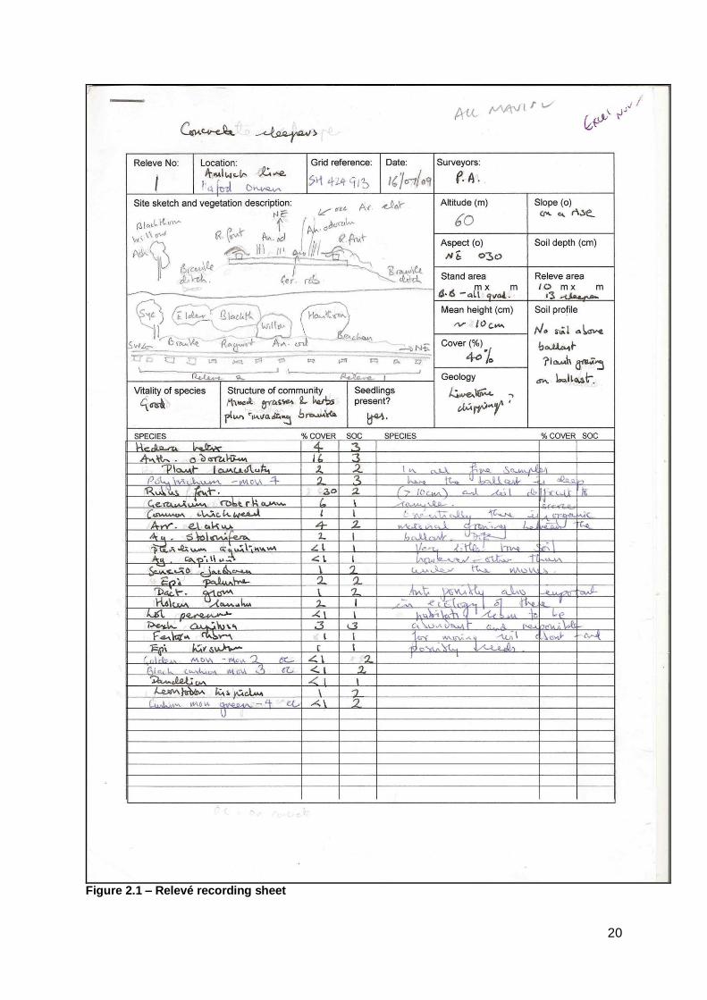
A field-recording sheet was created to input the raw data during the surveys (see
Figure 2.1) which included space for environmental data and a sketch of the railway
line. The field-recording sheet was created using aspects of the NVC recording
sheet.
At each site, each plant was identified within the relevé. In general, the percentage
cover of each plant was recorded, to enable subsequent MAVIS analysis. For the
NVC tables, the percentage covers were converted into NVC Domin scores:
NVC Domin Scores
10 Cover of 91-100%
9 76-90%
8 51-75%
7 34-50%
6 26-33%
5 11-25%
4 4-10%

19
3 with many individuals
2 with several individuals
1 with few individuals
In all cases, if plants, particularly non-vascular plants, could not be identified in the
field then a small sample of the plant was collected for subsequent identification (i.e.
with a microscope and relevant keys). Vascular plants were named following Stace
(2010) and bryophytes using Smith (2004). The NVC community names (Rodwell,
1991-2000) were followed despite some including species names that have since
been updated. An asterix in the results tables indicates where a name is new which
does not correspond to the NVC species name. Microspecies were identified only to
the aggregate level. In some cases, it was not possible to identify plants beyond
genus due to their recent germination and small size. These are included within the
NVC tables but are not included within the species totals.
20
Figure 2.1 – Relevé recording sheet

21
176 relevés were taken from a total of 35 sites from 22 different railway lines (see
Table 2.1).
TABLE 2.1 LIST OF RAILWAY LINE SITES SURVEYED
SITE GRID REFERENCE
VICE-COUNTY
NO OF RELEVES
DATE SURVEYED
Amlwch SH 424913 52 5 16/07/2009
Appleby Cutting NY 694200 69 4 13/07/2009
Appleby Embankment NY 696195 69 4 13/07/2009
Appleby Wet NY 694199 69 3 13/07/2009
Blaenau Ffestiniog Cutting SH 705441 48 6 16/09/2009
Blaenau Ffestiniog Embankment SH 707439 48 5 16/09/2009
Blaenau Ffestiniog Open SH 704443 48 3 16/09/2009
Cambridge TL 428639 29 5 23/08/2004
Carrington SJ 753903 58 10 04/05/2007
Fleetwood North SD 328457 60 5 07/07/2009
Fleetwood South SD 342428 60 5 07/07/2009
Gobowen – Oswestry SJ300313 40 5 17/07/2009
Golborne Ash SJ 603993 59 3 03/08/2009
Golborne North SJ 602991 59 5 03/08/2009
Golborne Sidings SJ 603989 59 6 04/08/2004
Golborne South SJ 601988 59 5 03/08/2009
Histon – St. Ives East TL 397681 29 3 21/07/2007
Histon – St. Ives West TL 363694 29 5 21/07/2007
Leek – Cauldon Quarry SK 022538 39 10 12/05/2005
Leek – Cauldon Quarry Wooded SJ 996545 39 3 12/05/2005
Leek – Stoke SJ 939538 39 6 04/05/2005
Newport – Ebbw Vale ST 210965 41 3 22/06/2007
Oswestry North Embankment SJ 297302 40 5 17/07/2009
Runcorn Docks SJ 499823 58 10 23/07/2009
St. Helens Acid Works SJ 527938 58 5 29/07/2004
St. Helens Canal North SJ 515950 59 5 06/07/2009
St. Helens Canal South SJ 517949 59 5 06/07/2009
St. Helens Link SJ 527939 58 4 21/06/2004
Staveley North SK 440741 57 5 22/08/2009
Staveley South SK 442739 57 5 22/08/2009
Trecwn East SM 963324 45 3 10/09/2010
Trecwn West SM 956320 45 5 10/09/2010
Wirksworth Quarry SK 288545 57 3 18/07/2004
Woodthorpe Colliery SK 459744 57 5 13/08/2009
Woodthorpe Colliery Junction SK 456742 57 5 13/08/2009
2.2.3 NVC Analysis
Once each site had been sampled, floristic tables were produced from the botanical
data. The frequency of each species was calculated and given a Roman numeral
value between I and V; I = occurs between 1 and 20% of samples, II = 21-40%, III =
41-60%, IV = 61-80% and V = found in between 81-100% of quadrats sampled.
Constant species were identified which form the backbone of the community. A
22
constant species is a species which occurs in 61 to 100% of the quadrats, identified
by the Roman numerals IV and V. A frequency of III is classed as a common or
frequent species, II is classed as an occasional species and I as a scarce species.
Following the production of the NVC tables and the identification of the constant
species, each community was analysed using three approaches; the MAVIS
similarity programme, multivariate analysis and keying out using the NVC books with
associated reading of the relevant literature. Each table was analysed using the
Modular Analysis of Vegetation Information System (MAVIS) software (CEH). MAVIS
analyses the data and attempts to classify each site into an NVC community. MAVIS
works by computing a similarity co-efficient for each NVC community based on
Sorenson’s Similarity Co-efficient. MAVIS does not take into account the Domin
scores of each species within each community. It is based only on shared presence
of a species.
Correspondence Analysis (CA) was also used to analyse the communities. All of the
communities were inputted to a MultiVariate Statistical Package (MVSP) programme
(Kovach, Version 3) along with four NVC communities, chosen because of their
frequency within the MAVIS results or by keying out the communities.
Correspondence Analysis (CA) was chosen within MVSP.
TWINSPAN analysis was undertaken with default settings and the cut levels are 2
and 5 (as in Lockton & Whild, 2014). The mean and standard deviation of Ellenberg
indicator values for Light, Werness, pH and Fertlity were calculated (Ellenberg ref) as

23
were the man and standard deviation for CSR values (Grime et al, 1988) for the end
groups identified by TWINSPAN.
In addition to MAVIS, CA and TWINSPAN, each site’s NVC table was keyed out by
hand using the published NVC Volumes 1 to 5. Once keyed out the relevant
chapters were read carefully and a detailed comparison between each published
NVC table and each sites NVC table was made. Comparison against the known
distribution of each published NVC community and their habitat description and
physiognomy was also undertaken.
Following this analysis, a decision was then made to allocate an NVC category for
each railway community or decide that no NVC community could be allocated.
24
2.3 RESULTS
2.3.1 Correspondence Analysis (CA)
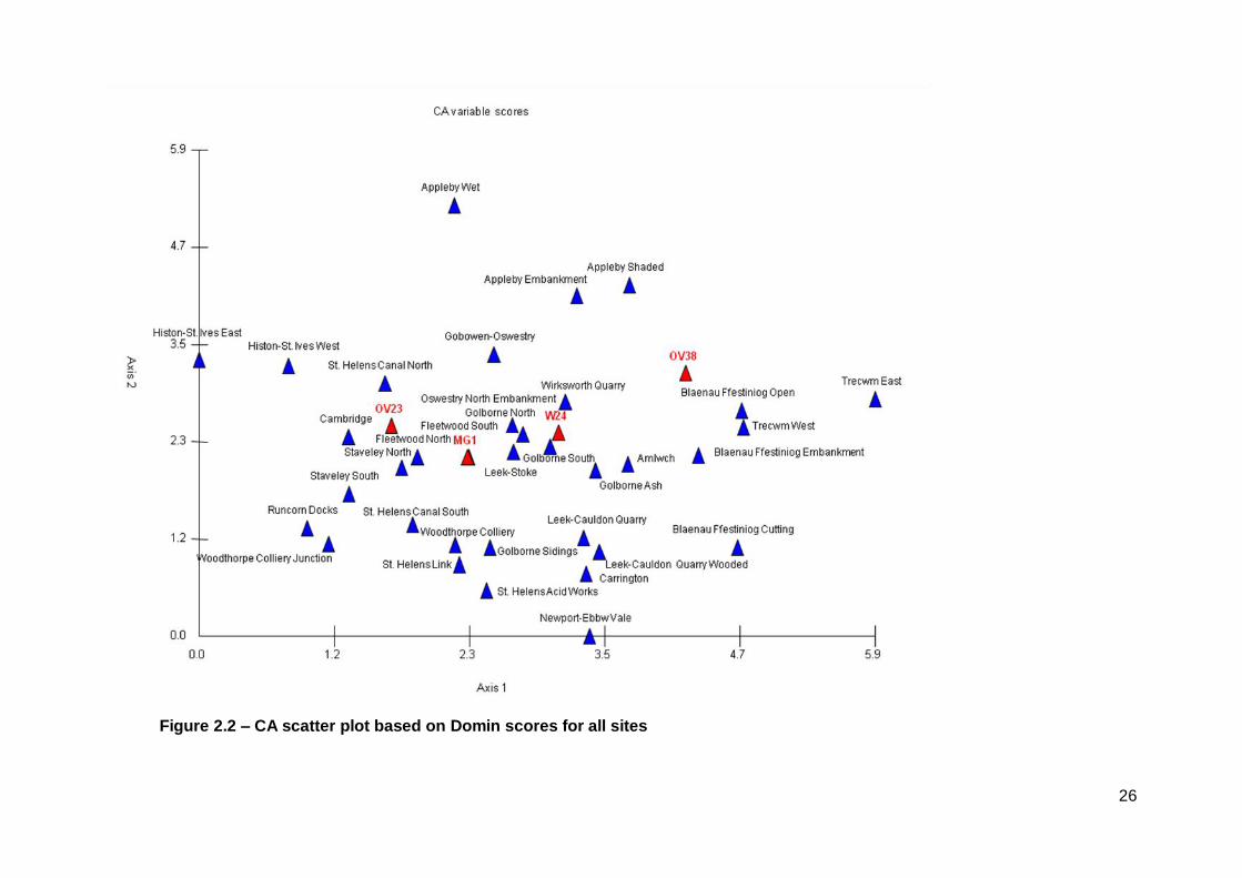
The results reveal different community composition between sites (see Figure 2.2).
This is reflected in the CA result that shows a broad scatter of results with some
communities close to those published. The strengths of these affinities are detailed
within the account of each site below. Three of the four published communities are
located centrally and relatively closely (OV23, MG1 and W24). The fourth community
(OV38) is slightly more distant. All of the published communities are separated by
the first axis.
Twinspan identified seven end groups in the stand analysis (Groups 1, 000, 001,
011, 0101, 01000 and 01001 - see Figure 2.3), with up to four indicator species in
each group. The full data is included in the appendix. Arrhenatherum elatius appears
as an indicator species in two groups (Group 1 and Group 01001). In Group 1 it is
the sole indicator species and is found with preferential species including shrubs and
scrub (Acer pseudoplatanus, Rubus fruticosus agg., Calluna vulgaris, Ulex gallii),
grasses (Holcus lanatus) and large forbs (Hypericum tetrapterum and Angelica
sylvestris). In Group 01001, Arrhenatherum elatius is identified as an indicator
species along with Epilobium montanum, Rubus fruticosus agg., and Brachythecium
rutabulum. Preferential species in this group includes the shrub Buddleja davidii,
grasses (Elytrigia repens, Poa pratensis) and forbs (Epilobium ciliatum).
The Ellenberg indicator table values show little simple separation between groups,
as does the CSR data (Table 2.2). The full TWINSPAN data set is included in
Appendix 4. All groups are comprised of mainly competitors or stress tolerators. The

25
two groups with Arrhenatherum elatius (1 and 01001), occupy the higher fertility end,
a range of pH, at the higher end of the wetness scale and a range of light values.
Both have comparable values of competitive species and stress tolerators but Group
1 has a much higher ruderal value than Group 01001. Indeed these reflect the
highest and lowest values of all groups.
26
Figure 2.2 – CA scatter plot based on Domin scores for all sites

27
Figure 2.3 Twinspan analysis of 174 relevés with a total of 273 species

28
TABLE 2.2 FULL ECOLOGICAL DATA SET
Group n Light Wetness pH Fertility C S R
1 14 Mean 6.39 5.89 5.99 5.61 2.49 2.24 3.10
st dev 0.40 0.66 0.18 0.40 0.39 0.26 0.27
000 34 Mean 6.94 5.13 6.27 5.28 2.82 2.14 2.73
SD 0.26 0.26 0.27 0.37 0.31 0.19 0.18
001 22 Mean 6.92 5.63 6.47 5.61 3.08 2.08 2.55
SD 0.15 0.46 0.27 0.47 0.41 0.18 0.30
011 16 Mean 7.06 4.93 6.49 5.23 2.70 2.16 2.93
SD 0.27 0.27 0.19 0.45 0.29 0.13 0.22
0101 28 Mean 6.93 5.36 6.13 5.19 3.06 2.32 2.69
SD 0.20 0.20 0.23 0.38 0.29 0.26 0.33
01000 17 Mean 6.54 5.54 5.84 5.02 3.09 2.42 2.47
SD 0.30 0.39 0.52 0.53 0.24 0.24 0.29
01001 43 Mean 6.76 5.48 6.16 5.52 3.42 2.10 2.29
SD 0.44 0.39 0.49 0.65 0.43 0.43 0.40

29
2.3.2 NVC Analysis
The following pages show the NVC tables for each community sampled and a
discussion of the NVC result from MAVIS and from comparing the existing
NVC tables in each volume. Table 2.38 gives an overview of the results from
each site.
2.3.2.1 Amlwch
TABLE 2.3 AMLWCH
SPECIES/RELEVE 1 2 3 4 5 F
Hedera helix 4 4 4 4 2 V
Anthoxanthum odoratum 5 5 6 5 5 V
Plantago lanceolata 2 1 2 1 5 V
Rubus fruticosus agg. 6 5 4 4 4 V
Arrhenatherum elatius 4 2 2 2 1 V
Senecio jacobaea 1 1 1 1 1 V
Dactylis glomerata 1 2 4 4 1 V
Festuca rubra 1 1 4 1 1 V
Polytrichum commune var. commune 2 1 4 4 IV
Agrostis capillaris 1 5 4 4 IV
Holcus lanatus 2 4 4 2 IV
Geranium robertianum 4 1 1 III
Brachythecium rutabulum 1 1 4 III
Schistidium crassipilum 1 2 1 III
Atrichum undulatum 1 4 4 III
Linaria vulgaris 1 1 1 III
Campylopus introflexus 1 4 4 III
Agrostis stolonifera 2 1 II
Lolium perenne 1 1 II
Deschampsia cespitosa 3 1 II
Leontodon hispidus 1 1 II
Bryum capillare 1 1 II
Hieraceum sp. 1 4 II
Stellaria media 1 I
Pteridium aquilinum 1 I
Epilobium palustre 2 I
Epilobium hirsutum 1 I
Taraxacum officinale agg. 1 I
Epilobium parviflorum 1 I
Veronica officinalis 1 I
Ceratodon purpureus 2 I
Carex flacca 1 I
Lotus corniculatus 1 I
Equisetum arvense 1 I
Rumex acetosa 1 I
Epilobium montanum 1 I

30
TOTAL SPECIES: 36 24 17 16 19 19
Top four MAVIS results: FIT MG9b 48.3 MG1a 43.8 MG9 42.0 MG1e 41.7
The Amlwch line was situated on relatively flat ground and was surrounded by
farmland. The community was mainly grass species with some low-growing
herbaceous species and Bramble encroaching across the track. The
vegetation cover was 50% on average. A total of 36 species were recorded.
Eleven species were classed as constants. These included Hedera helix,
Anthoxanthum odoratum and Polytrichum commune var. commune. Six of the
eleven constants were grass species.
The CA analysis shows that Amlwch plot is closer to W24 than the other three
NVC communities. This is not borne out by the species present at this site.
The top MAVIS result for Amlwch was MG9b Holcus lanatus–Deschampsia
cespitosa grassland Arrhenatherum elatius sub-community. MG9 is a
community of rank, tussocky grasses typical of permanently moist or
periodically inundated neutral soils (Rodwell, 1994). The constants within the
Amlwch community matched some of the constants within MG9b. However,
the Amlwch community is free-draining and MG9 is a marshy grassland
community so MG9 is discounted. MG1a Arrhenatherum elatius grassland
Festuca rubra sub-community is a better match, MG1 being a community
typical of well-drained unmanaged land and for the fact that Holcus lanatus
was not recorded from within every quadrat at Amlwch albeit still attaining a

31
constant status. The number of constant grass species also pushes this
community towards MG1a. MG1 was the second and fourth result in MAVIS.
However, the Amlwch community does not support the large Umbellifer
species that form a constituent of MG1, probably because this community has
developed from a pioneer ruderal community, rather than an unmanaged
grassland community with more established soil. The CA analysis also shows
that Amlwch is not close to MG1. Amlwch is classed as having elements of
MG1 but lacking the Umbellifer species.

32
2.3.2.2 Appleby Embankment
TABLE 2.4 APPLEBY EMBANKMENT
SPECIES/RELEVE 1 2 3 4 F
Barbula convoluta 4 2 1 4 V
Schistidium crassipilum 4 4 4 4 V
Urtica dioica 1 1 1 1 V
Epilobium montanum 1 1 2 1 V
Lolium perenne 1 4 4 4 V
Cardamine hirsuta 1 1 1 1 V
Schistidium apocarpum s.s. 4 3 4 2 V
Brachythecium rutabulum 1 1 2 2 V
Arabidopsis thaliana 1 1 1 IV
Lathyrus pratensis 1 1 1 IV
Leucanthemum vulgare 1 1 1 IV
Ceratodon purpureus 1 1 4 IV
Sonchus oleraceus 1 1 1 IV
Kindbergia praelonga 1 2 4 IV
Festuca rubra 4 4 2 IV
Dactylis glomerata 1 2 III
Agrostis capillaris 1 1 III
Myosotis discolor 1 1 III
Scorzoneroides autumnalis 1 1 III
Holcus lanatus 2 1 III
Galium album* (Galium mollugo) 1 1 III
Equisetum arvense 4 4 III
Deschampsia cespitosa 2 4 III
Myosotis arvensis 3 2 III
Geum urbanum 1 II
Fraxinus excelsior (sap) 1 II
Grimmia pulvinata 1 II
Calliergonella cuspidata 1 II
Tortula muralis 1 II
Hypochaeris radicata 1 II
Glechoma hederacea 1 II
Geranium robertianum 4 II
Poa pratensis 4 II
Lapsana communis 1 II
Sagina procumbens 1 II
Senecio vulgaris 1 II
TOTAL SPECIES: 36 18 26 23 16
Top four MAVIS results: FIT W24b 36.9 W24 34.6 MG6 32.7 OV23 31.8
The Appleby Embankment site was situated on a low embankment,
surrounded by permanent pasture. The ballast was open with a low coverage

33
of vegetation (on average 30% cover). The community comprised mainly low-
growing herbaceous species with many bryophytes. A total of 36 species
were recorded from here with fifteen constant species. Constants included six
species of bryophyte along with Epilobium montanum, Urtica dioica,
Arabidopsis thaliana and Lathyrus pratensis.
The CA shows the Appleby Embankment plot as distant from any of the NVC
communities. The top MAVIS result for Appleby Embankment was W24b
Rubus fruticosus–Holcus lanatus underscrub Arrhenatherum elatius–
Heracleum sphondylium sub-community. While this community is typical of
abandoned and neglected ground (Rodwell, 1991), the presence of only two
W24 constant species at the site (Urtica dioica and Festuca rubra), in addition
to the lack of Rubus fruticosus agg., led to this community allocation being
rejected. Other MAVIS results can also be eliminated. MG6 Lolium perenne–
Cynosurus cristatus grassland occurs on free-draining ground and can be
found within the uplands as long as lime is added to maintain the Lolium
perenne. However, Cynosurus cristatus, a key element of the MG6
community is absent OV23 Lolium perenne–Dactylis glomerata community
was the fourth MAVIS result. This is a community of neglected but resown
habitats, with a closed sward. The Appleby community was an open
community with very little Dactylis glomerata. Therefore, the community at
Appleby Embankment cannot be matched with any existing NVC
community.

34
2.3.2.3 Appleby Shaded
TABLE 2.5 APPLEBY SHADED
SPECIES/RELEVE 1 2 3 4 F
Epilobium montanum 2 2 1 4 V
Schistidium crassipilum 4 5 5 4 V
Schistidium apocarpum s.s. 4 4 4 2 V
Geranium robertianum 4 2 1 1 V
Cardamine flexuosa 2 5 4 4 V
Urtica dioica 1 1 1 1 V
Sonchus oleraceus 1 1 1 IV
Acer pseudoplatanus (sap) 1 1 III
Hypnum cupressiforme 1 1 III
Cardamine hirsuta 2 II
Hypericum pulchrum 1 II
Geum urbanum 1 II
Hypnum cupressiforme 1 II
Lolium perenne 1 II
Calliergonella cuspidata 1 II
Barbula convoluta 1 II
Rumex acetosa 1 II
Chamerion angustifolium 1 II
Leucanthemum vulgare 1 II
Galium album* (Galium mollugo) 1 II
Epilobium parviflorum 1 II
Sagina procumbens 1 II
Lathyrus pratensis 1 II
Poa pratensis 2 II
Veronica beccabunga 1 II
Deschampsia cespitosa 1 II
Tussilago farfara 1 II
TOTAL SPECIES: 26 11 13 10 15
Top four MAVIS results: FIT OV27 24.3 W24 24.0 W24b 23.7 MG1b 23.0
The Appleby Shaded site was situated within a cutting with dense woodland
on the slopes. It was a damp, shaded community. The vegetation was a
mixture of low-growing herbaceous species, open ballast, minimal grass cover
and six species of bryophyte. The vegetation cover over the ballast was low
(average of 30%). A total of 26 species were recorded from here, eight of
35
those were constants, including Geranium robertianum, Sonchus oleraceus
and two species of bryophyte.
The CA shows the Appleby Shaded plot as distant from any NVC community.
The top MAVIS result for Appleby Shaded was OV27 Epilobium angustifolium
community, with W24 and W24b Rubus fruticosus–Holcus lanatus underscrub
Arrhenatherum elatius–Heracleum sphondylium sub-community closely
following. None of these communities fit the Appleby Shaded community due
to the lack of matching species. For example, Chamerion angustifolium,
Rubus fruticosus agg. or Holcus lanatus did not occur in any sample at this
site. Similarly, the fourth MAVIS result of MG1 can be discounted due to the
lack of Arrhenatherum elatius in the community. The Appleby Shaded
community cannot be placed within any existing NVC community.

36
2.3.2.4 Appleby Wet
TABLE 2.6 APPLEBY WET
SPECIES/RELEVE 1 2 3 F
Veronica beccabunga 4 2 1 V
Cardamine flexuosa 4 2 4 V
Urtica dioica 1 1 2 V
Epilobium montanum 1 2 1 V
Alliaria petiolata 1 1 1 V
Lolium perenne 1 1 2 V
Agrostis stolonifera 1 1 1 V
Stellaria media 1 1 IV
Sagina procumbens 2 5 IV
Poa annua 1 1 IV
Solanum dulcamara 1 1 IV
Chamerion angustifolium 1 II
Juncus articulatus 1 II
Epilobium palustre 1 II
Galium palustre 1 II
Holcus lanatus 1 II
Juncus bufonius 1 II
Galium aparine 1 II
Brachythecium rivulare 1 II
Geranium robertianum 1 II
Kindbergia praelonga 1 II
Tussilago farfara 1 II
Ranunculus bulbosus 1 II
Senecio jacobaea 1 II
Barbula convoluta 1 II
Ceratodon purpureus 1 II
Galium saxatile 1 II
Plantago major 1 II
Leucanthemum vulgare 1 II
Myosotis arvensis 1 II
Epilobium parviflorum 2 II
Arabidopsis thaliana 1 II
TOTAL SPECIES: 32 12 17 21
Top four MAVIS results: FIT OV10c 33.8 OV10 33.1 OV20b 33.1 OV23 32.7
The Appleby Wet site was situated within a cutting, with dense woodland and
scrub on the slopes either side of the track. The community was a mixture of
ruderal species and bryophytes with taller vegetation nearer to the rails. This
section of track was more open than Appleby Shaded, with a less dense

37
canopy shading the track. Vegetation cover was very low on the ballast with
an average of 15% cover. A total of 32 species were recorded including
eleven constants. Constants included Veronica beccabunga, Alliaria petiolata
and Solanum dulcamara.
The CA shows the Appleby Wet plot as extremely distant from any of the four
NVC communities. The top MAVIS result for the Appleby Wet site was OV10c
Poa annua–Senecio vulgaris community Agrostis stolonifera–Rumex crispus
sub-community. The NVC table for OV10c matched the constant Poa annua
from the Appleby Wet community. However Senecio vulgaris was not present
in this community and OV10 is typical of fertile habitats which are trampled or
disturbed, so ecologically does not match this site. When comparing the
tables, three constants were matched with OV20b Poa annua–Sagina
procumbens community Lolium perenne–Chamomilla suaveolens sub-
community (The constants being Poa annua, Sagina procumbens and Lolium
perenne). OV20 is typically a crevice community, occurring within paving
cracks and between cobbles; a hostile habitat with varying degrees of
moisture throughout the year which only certain species can tolerate. It was
also the third MAVIS fit. However, the ballast at Appleby Wet was dissimilar to
the OV20 habitats and the species assemblage was completely different.
OV23 Lolium perenne-Dactylis glomerata community was the fourth MAVIS
result. Dactylis glomerata did not occur at Appleby Wet and OV23 is typically
a closed sward community of fertile ground, Appleby Wet was an open
community of infertile ballast. None of these communities fitted the

38
community present at Appleby Wet and no NVC community can be
allocated.
39
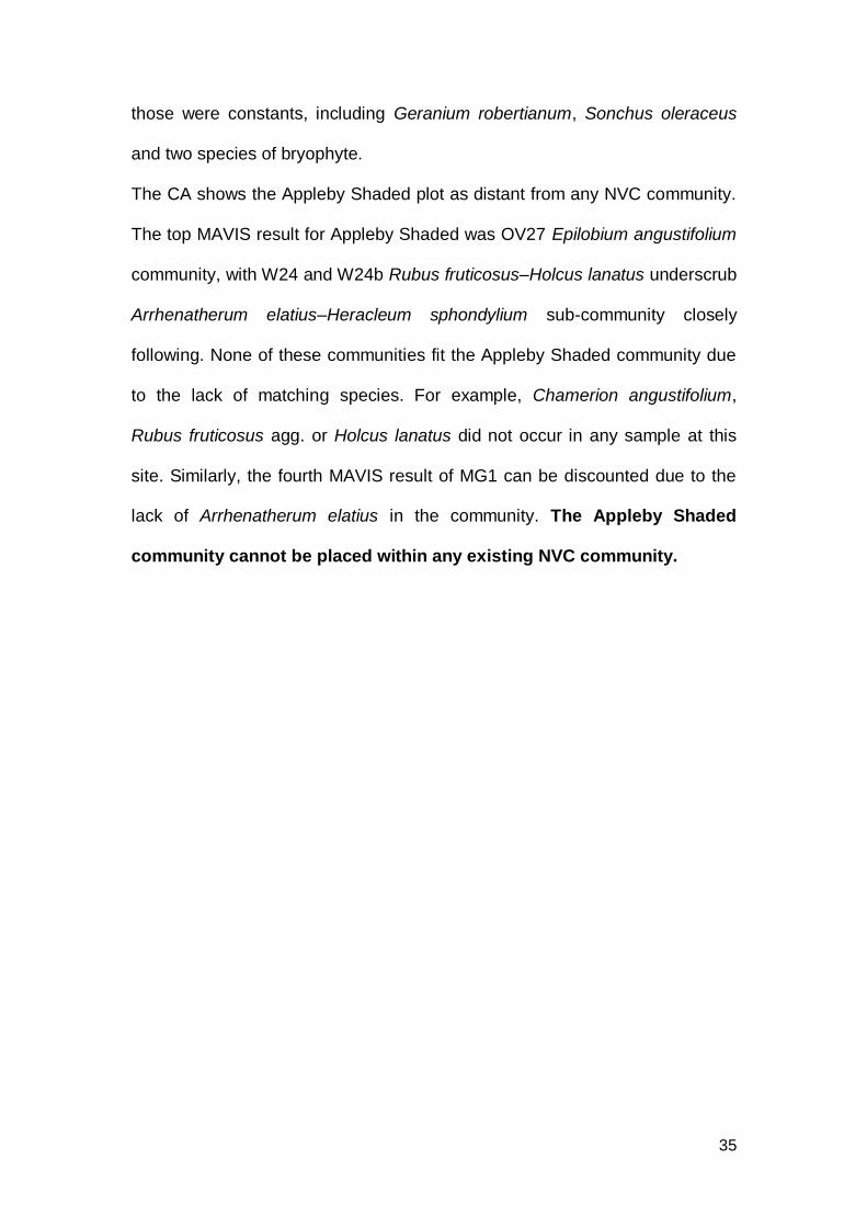
2.3.2.5 Blaenau Ffestiniog Cutting
TABLE 2.7 BLAENAU FFESTINIOG CUTTING
SPECIES/RELEVE 1 2 3 4 5 6 F
Arrhenatherum elatius 4 5 4 1 1 4 V
Fraxinus excelsior (sap) 5 5 5 6 7 7 V
Agrostis capillaris 1 1 1 1 1 V
Geranium robertianum 1 1 1 1 4 V
Epilobium ciliatum 1 1 1 1 1 V
Festuca rubra 5 4 1 1 IV
Rubus fruticosus agg. 5 5 7 4 IV
Dactylis glomerata 1 1 2 III
Rhododendron ponticum 1 2 2 III
Senecio jacobaea 1 1 1 III
Quercus robur (sap) 2 1 1 III
Hypericum pulchrum 1 1 II
Viola riviniana 1 1 II
Teucrium scorodonia 1 1 II
Holcus lanatus 1 1 II
Crataegus monogyna 1 1 II
Leycesteria formosa 1 4 II
Plantago lanceolata 1 1 II
Dryopteris felix-femina 1 1 II
Peltigera sp. 1 1 II
Buddleja davidii 4 4 II
Hieraceum umbellatum 1 I
Taraxacum officinale agg. 1 I
Luzula campestre 1 I
Digitalis purpurea 1 I
Asplenium trichomanes 1 I
Agrostis stolonifera 1 I
Lotus corniculatus 1 I
Leylandii 1 I
Hypochaeris radicata 1 I
Heracleum sphondylium 1 I
Sonchus asper 1 I
Solidago canadensis 2 I
Luzula sylvatica 1 I
Chamerion angustifolium 1 I
Urtica dioica 1 I
Dryopteris felix-mas 1 I
Rhytidiadelphus squarrosus 4 I
Juncus effusus 1 I
TOTAL SPECIES: 39 19 20 17 14 4 11
Top four MAVIS results: FIT MG1a 40.4 SD9a 39.7 W24 38.7 OV27 36.8

40
The Blaenau Ffestiniog Cutting site was situated within a deep cutting. To the
north was the bare slate cutting and to the south was a low mound covered in
trees and shrubs. This was a sheltered and shaded site. The community
comprised tall grass near to the rails with many Ash saplings scattered on the
ballast. A number of non-native species were present albeit with low cover
values. The vegetation covered more of the track than on the adjacent
embankment site with an average of 70% cover. A total of 39 species were
recorded. Seven species were recorded as constants including Geranium
robertianum, Fraxinus excelsior and Epilobium ciliatum.
The CA shows the Blaenau Ffestiniog Cutting plot as very distant from any of
the four NVC communities. The top MAVIS result from Blaenau Ffestiniog
Cutting was MG1a Arrhenatherum elatius grassland Festuca rubra sub-
community. This matches two constant species from the site: Arrhenatherum
elatius and Festuca rubra. Comparison to the existing NVC tables shows that
OV38 Gymnocarpietum robertianae community is a slightly better fit with three
constants being matched; Geranium robertianum, Arrhenatherum elatius and
Festuca rubra. However, Gymnocarpium robertianum was not present on this
site. Moreover this is a Northern England limestone scree community. With
ballast being granite this will give a calcifugous community, hence OV38 has
been omitted from consideration. Likewise the second MAVIS result, SD9a
Ammophila arenaria–Arrhenatherum elatius dune grassland typical sub-
community can also be discounted due to it being a dune community and due
to the lack of Ammophila arenaria on the site. OV27 Epilobium angustifolium
community can be discounted due to the tiny amount of Chamerion

41
(Epilobium) angustifolium present on the site. W24 Rubus fruticosus–Holcus
lanatus underscrub was the third MAVIS result and the site does have
affinities with this NVC community. Rubus fruticosus agg. is a constant and
records relatively high cover values in comparison with other species as does
Fraxinus excelsior (as saplings). This moves the community away from MG1
as Arrhenatherum elatius has lower cover values. However, the combination
of the other species present shows this community has elements of acid
heath to it with species occurring such as Rhododendron ponticum and
Luzula sylvatica. There are also a number of non-native species present such
as Leycesteria formosa and Buddleja davidii. Blaenau Ffestiniog Cutting
has affinities to W24 but with acidic heath and non-native constituents.

42
2.3.2.6 Blaenau Ffestiniog Embankment
TABLE 2.8 BLAENAU FFESTINIOG EMBANKMENT
SPECIES/RELEVE 1 2 3 4 5 F
Arrhenatherum elatius 6 5 5 4 5 V
Agrostis capillaris 1 1 1 1 1 V
Hypnum cupressiforme 1 1 1 2 2 V
Festuca ovina 1 1 1 5 IV
Viola riviniana 1 1 1 1 IV
Dactylis glomerata 1 1 1 III
Epilobium ciliatum 1 1 1 III
Teucrium scorodonia 4 4 1 III
Geranium robertianum 1 1 1 III
Holcus lanatus 2 1 II
Festuca rubra 2 2 II
Hypericum pulchrum 1 1 II
Heracleum sphondylium 1 1 II
Rhytidiadelphus squarrosus 1 I
Calliergonella cuspidata 1 I
Calluna vulgaris 1 I
Stellaria media 1 I
Taraxacum officinale agg. 1 I
Senecio jacobaea 1 I
Digitalis purpurea 1 I
Fraxinus excelsior (sap) 1 I
Hieraceum umbellatum 1 I
Pilosella officinarum 1 I
Hypochaeris radicata 1 I
Plantago lanceolata 1 I
Epilobium parviflorum 1 I
TOTAL SPECIES: 26 10 9 9 17 11
Top four MAVIS results: FIT SD9a 38.4 W23 38.2 MG1a 38.1 W24 36.9
The Blaenau Ffestiniog Embankment site was situated on a slight
embankment. The surrounding land was farmland and heathland. The ballast
was open and the average vegetation cover was 40%. The site was
dominated by Arrhenatherum elatius which tended to grow near to the rails.
Low growing herbaceous species and bryophytes occurred sporadically on
the ballast. A total of 26 species were recorded with five of these being

43
constant species. Constants included Hypnum cupressiforme and Festuca
ovina.
The CA shows the Blaenau Ffestiniog Embankment plot distant from any of
the NVC communities but in line with some other sites which have affinities to
MG1. The top MAVIS result from Blaenau Ffestiniog Embankment was SD9a
Ammophila arenaria–Arrhenatherum elatius dune grassland typical sub-
community. However, this community matched only Arrhenatherum elatius as
a constant species and ecologically did not fit. The only woodland feature is
the presence of Fraxinus excelsior saplings hence the W23 Ulex europaeus-
Rubus fruticosus scrub community and W24 Rubus fruticosus–Holcus lanatus
underscrub community designations are inappropriate. This is also reflected in
the distance of the Blaenau Ffestiniog Embankment plot from the W24 plot on
the CA plot. A closer match to an existing NVC community appeared to be
CG10a Festuca ovina–Agrostis capillaris–Thymus praecox grassland
Trifolium repens–Luzula campestris sub-community. This is a community of
calcareous bedrock and coarse-textured superficial deposits. CG10a also
matched three constants: Festuca ovina, Agrostis capillaris and Viola
riviniana. However, CG10a does not fit the community due to it being typically
a closed sward community that is heavily grazed and Thymus praecox does
not occur at the Blaenau Ffestiniog Embankment site, probably due to the
non-calcareous nature of the substrate. The assemblage here has affinities
with MG1a Arrhenatherum elatius grassland Festuca rubra sub-community
due to the dominance of Arrhenatherum elatius and the presence of other
grasses such as Agrostis capillaris and Dactylis glomerata. However, it does

44
lack other constituents of MG1a such as tall Umbellifers and the site supports
an acid heath element to it with species occurring such as Digitalis purpurea
and Calluna vulgaris. This community has affinities to MG1 but cannot be
placed within an existing MG1 sub-community.

45
2.3.2.7 Blaenau Ffestiniog Open
TABLE 2.9 BLAENAU FFESTINIOG OPEN
SPECIES/RELEVE 1 2 3 F
Molinia caerulea 7 6 7 V
Rubus fruticosus agg. 4 5 2 V
Holcus lanatus 4 5 6 V
Brachythecium rutabulum 4 4 4 V
Senecio jacobaea 1 1 1 V
Epilobium ciliatum 1 1 2 V
Fraxinus excelsior (sap) 4 4 4 V
Lolium perenne 2 2 IV
Agrostis capillaris 2 2 IV
Rhododendron ponticum 1 1 IV
Epilobium parviflorum 1 1 IV
Geranium robertianum 1 1 IV
Betula pubescens (sap) 2 2 IV
Dryopteris felix-mas 1 II
Dryopteris felix-femina 1 II
Arrhenatherum elatius 1 II
Vaccinium myrtillus 1 II
Rhytidiadelphus squarrosus 3 II
Plantago lanceolata 1 II
Festuca rubra 2 II
Rumex acetosa 1 II
Juncus articulatus 1 II
Calluna vulgaris 1 II
TOTAL SPECIES: 23 12 16 15
Top four MAVIS results: FIT W23b 30.7 MG6b 29.4 MG9 28.5 MG9b 28.3
The Blaenau Ffestiniog Open site was situated within a shallow cutting. The
track was more open to the light than the Blaenau Ffestiniog Cutting site. The
site was wet, from run-off from the surrounding slate cutting and had elements
of heath within the species assemblage. The community was a mixture of tall
grass growing close to the rails, with single pioneer shrub species and
Bramble encroaching across the ballast. Mean vegetation cover was 60%. A
total of 23 species were recorded with thirteen of these being constants.

46
Constants included Molina caerulea, Rhododendron ponticum, Brachythecium
rutabulum and Epilobium parviflorum.
The CA shows the Blaenau Ffestiniog Open plot close to OV38
Gymnocarpietum robertianum-Arrhenatherum elatius community. This can be
discounted because OV38 is a community of limestone uplands. The top
MAVIS result for Blaenau Ffestiniog Open was W23b Ulex europaeus–Rubus
fruticosus scrub Rumex acetosella sub-community. The lack of Ulex
europaeus means W23 does not match this community. The Blaenau
Ffestiniog Open community supported Molinia caerulea as a constant
species. Molinia caerulea features in the heathland communities, which is not
reflected in other constituents of this community. MG6b Lolium perenne-
Cynosurus cristatus grassland Anthoxanthum odoratum community was the
second MAVIS result. However MG6 is a permanent pasture community with
many grasses and no heathland characteristics. MG9 Holcus lanatus-
Deschampsia cespitosa grasslands were also identified as matches by
MAVIS. Deschampsia cespitosa did not occur at the site and MG9 is typically
a closed and stable grassland sward of permanently moist soils. Thus MG9
does not match the Blaenau Ffestiniog Open community. Due to the
combination of heath species, tree saplings and calcifugous species, no
existing NVC communities can be matched to this community.
47
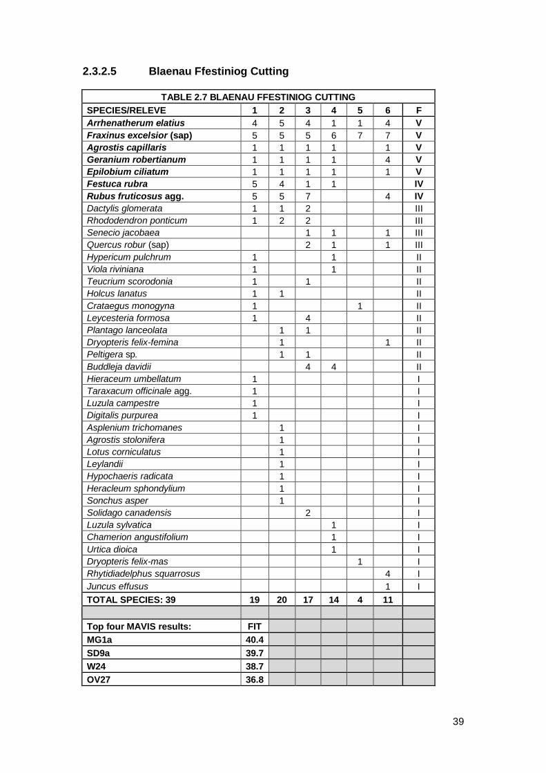
2.3.2.8 Cambridge
TABLE 2.10 CAMBRIDGE
SPECIES/RELEVE 1 2 3 4 5 F
Achillea millefolium 7 7 5 5 7 V
Lolium perenne 5 7 5 7 5 V
Artemisia vulgaris 3 1 3 4 2 V
Arrhenatherum elatius 3 3 5 3 3 V
Trifolium campestre 5 1 2 3 2 V
Conyza canadensis 3 3 3 3 3 V
Senecio jacobaea 1 2 3 3 3 V
Festuca rubra 4 5 4 7 7 V
Rubus fruticosus agg. 6 6 4 2 IV
Crepis capillaris 4 2 2 1 IV
Dactylis glomerata 4 3 5 3 IV
Calystegia sepium 3 1 3 3 IV
Poa pratensis 1 3 2 1 IV
Plantago lanceolata 1 3 3 III
Tragopogon pratensis 1 1 1 III
Sagina procumbens 3 3 1 III
Leucanthemum vulgare 1 2 3 III
Chamerion angustifolium 1 1 1 III
Taraxacum officinale 2 2 2 III
Scorzoneroides autumnalis 2 1 2 III
Deschampsia flexuosa 1 1 II
Nardus stricta 1 1 II
Aira caryophylla 1 1 II
Hypochaeris radicata 1 1 II
Rumex acetosa 3 1 II
Anisantha sterilis 1 1 II
Matricaria discoidea 1 I
Heracleum sphondylium 1 I
Hypericum perforatum 1 I
Stellaria media 2 I
Rosa canina agg. 1 I
Agrostis stolonifera 1 I
Elytrigia repens 4 I
Hedera helix 1 I
Cirsium arvense 1 I
Succisa pratensis 1 I
TOTAL SPECIES: 36 22 19 18 25 19
Top four MAVIS results: FIT MG1a 42.6 OV23 42.3 OV23d 41.1 SD9a 41.0
The Cambridge site was situated in an open aspect on level ground bordered
by arable farmland. The line tended to exhibit tall vegetation near to the rails

48
with shorted vegetation towards the centre of the track and patches of open
ballast. A total of 36 species were recorded from this site and this included
thirteen constant species. Constants included Achillea millefolium and
Arrhenatherum elatius along with ruderal species such as Conyza
canadensis, Artemisia vulgaris and Calystegia sepium. All constants
exhibited low to medium cover.
The CA shows the Cambridge plot as being close to OV23 Lolium perenne–
Dactylis glomerata community. The top MAVIS result for Cambridge was to
MG1a Arrhenatherum elatius grassland Festuca rubra sub-community.
Second best fit in MAVIS was OV23. Both of these communities have
constant species which match some of the constants at Cambridge, for
example, Dactylis glomerata, Lolium perenne and Arrhenatherum elatius.
However, one constant at Cambridge was Achillea millefolium and this is a
constant species in OV23d. The fourth match (SD9a Ammophila arenaria–
Arrhenatherum elatius dune grassland typical sub-community) can be
discounted as Ammophila arenaria is absent. This community is classed as
OV23d Lolium perenne–Dactylis glomerata community Arrhenatherum
elatius-Medicago lupulina sub-community, given the number of ruderal
species present.
49
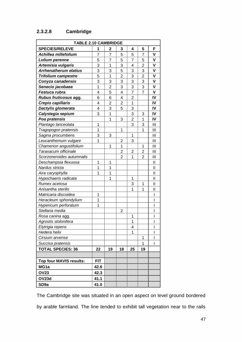
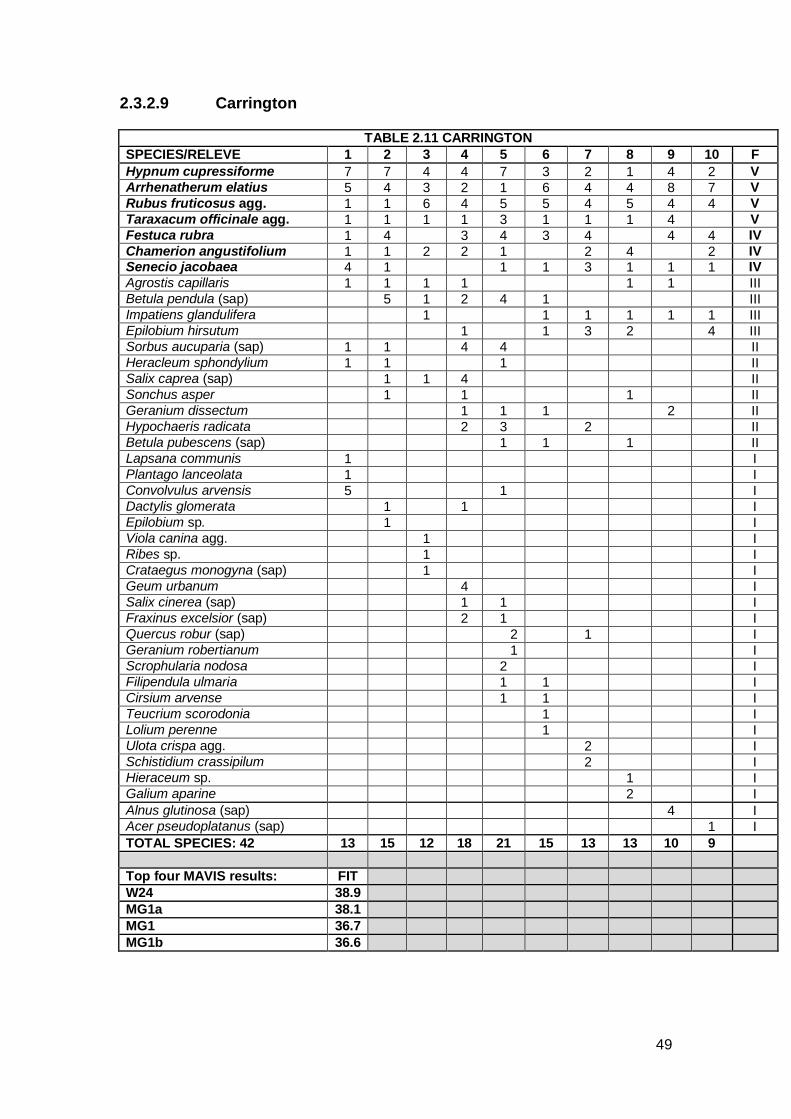
2.3.2.9 Carrington
TABLE 2.11 CARRINGTON
SPECIES/RELEVE 1 2 3 4 5 6 7 8 9 10 F
Hypnum cupressiforme 7 7 4 4 7 3 2 1 4 2 V
Arrhenatherum elatius 5 4 3 2 1 6 4 4 8 7 V
Rubus fruticosus agg. 1 1 6 4 5 5 4 5 4 4 V
Taraxacum officinale agg. 1 1 1 1 3 1 1 1 4 V
Festuca rubra 1 4 3 4 3 4 4 4 IV
Chamerion angustifolium 1 1 2 2 1 2 4 2 IV Senecio jacobaea 4 1 1 1 3 1 1 1 IV
Agrostis capillaris 1 1 1 1 1 1 III Betula pendula (sap) 5 1 2 4 1 III Impatiens glandulifera 1 1 1 1 1 1 III Epilobium hirsutum 1 1 3 2 4 III Sorbus aucuparia (sap) 1 1 4 4 II Heracleum sphondylium 1 1 1 II Salix caprea (sap) 1 1 4 II Sonchus asper 1 1 1 II Geranium dissectum 1 1 1 2 II Hypochaeris radicata 2 3 2 II Betula pubescens (sap) 1 1 1 II Lapsana communis 1 I Plantago lanceolata 1 I Convolvulus arvensis 5 1 I Dactylis glomerata 1 1 I Epilobium sp. 1 I Viola canina agg. 1 I Ribes sp. 1 I Crataegus monogyna (sap) 1 I Geum urbanum 4 I Salix cinerea (sap) 1 1 I Fraxinus excelsior (sap) 2 1 I Quercus robur (sap) 2 1 I Geranium robertianum 1 I Scrophularia nodosa 2 I Filipendula ulmaria 1 1 I Cirsium arvense 1 1 I Teucrium scorodonia 1 I Lolium perenne 1 I Ulota crispa agg. 2 I Schistidium crassipilum 2 I Hieraceum sp. 1 I Galium aparine 2 I
Alnus glutinosa (sap) 4 I Acer pseudoplatanus (sap) 1 I
TOTAL SPECIES: 42 13 15 12 18 21 15 13 13 10 9
Top four MAVIS results: FIT W24 38.9 MG1a 38.1 MG1 36.7 MG1b 36.6

50
The Carrington site was situated on a low embankment, surrounded by arable
land. The vegetation covered, on average, 70% of the ballast. The community
comprised tall grasses close to the rails with Bramble encroaching across the
ballast and many ruderal species. A total of 42 species were recorded. This
included seven constant species, including Hypnum cupressiforme,
Chamerion angustifolium, Taraxacum officinale agg. and Senecio jacobaea.
This community included many species of tree sapling such as Alnus
glutinosa, Quercus robur and Sorbus aucuparia.
The CA shows the Carrington plot as equidistant between W24 Rubus
fruticosus-Holcus lanatus underscrub and MG1 Arrhenatherum elatius
grassland, albeit some distance from either. The top MAVIS result for
Carrington was W24. This is due to Rubus fruticosus agg. being found in
every relevé. Comparison with the published NVC tables shows that W24
matches three constant species with Carrington; Rubus fruticosus agg.,
Arrhenatherum elatius and Taraxacum officinale agg. The Carrington
community also has elements of MG1 with Arrhenatherum elatius a constant
species plus other grass species. Due to the constant Chamerion (Epilobium)
angustifolium, the OV communities were analysed and OV27e Epilobium
angustifolium community Ammophila arenaria sub-community also matches
three constant species; Chamerion angustifolium, Festuca rubra and Senecio
jacobaea. However, the Carrington community appears more akin to a
grassland, with greater similarities to MG1 more so than W24, due to the
number of grass species present and the presence of a tall Umbellifer

51
(Heracleum sphondylium). Therefore, Carrington is classed as having
affinities to MG1.

52
2.3.2.10 Fleetwood North
TABLE 2.12 FLEETWOOD NORTH
SPECIES/RELEVE 1 2 3 4 5 F
Rubus fruticosus agg. 5 5 4 5 4 V
Taraxacum officinale agg. 2 1 2 2 1 V
Leucanthemum vulgare 4 5 4 4 4 V
Leontodon hispidus 4 2 4 4 2 V
Arrhenatherum elatius 4 3 3 1 2 V
Epilobium parviflorum 1 4 2 1 1 V
Senecio jacobaea 3 1 4 4 IV
Epilobium palustre 1 1 1 1 IV
Festuca ovina 4 1 1 2 IV
Potentilla reptans 1 4 2 III
Dactylis glomerata 1 1 1 III
Festuca rubra 5 8 2 III
Bromus hordeaceus 4 1 1 III
Hieraceum sp. 1 1 1 III
Vicia sativa 1 4 1 III
Ceratodon purpureus 1 1 1 III
Convolvulus arvensis 1 1 1 III
Vicia cracca 1 2 II
Geranium robertianum 1 4 II
Brachythecium rutabulum 4 4 II
Holcus lanatus 1 2 II
Sedum rupestre 2 4 II
Anisantha sterilis 2 1 II
Cladonia sp. 1 1 II
Plantago lanceolata 1 1 II
Helminthotheca echioides* (Picris) 1 1 II
Myosotis discolor 1 1 II
Linum catharticum 1 1 II
Cirsium arvense 1 1 II
Epilobium montanum 1 2 II
Valeriana officinalis 4 5 II
Sonchus arvensis 1 2 II
Salix caprea (sap) 1 I
Achillea millefolium 1 I
Sonchus oleraceus 1 I
Lapsana communis 4 I
Daucus carota 3 I
Trifolium campestre 1 I
Bryum caespiticium 1 I
Centaurea nigra 1 I
Chamerion angustifolium 1 I
Bryum sp. 1 I
Cerastium fontanum 1 I
Crataegus monogyna (sap) 1 I
Rumex acetosa 1 I
Galium aparine 1 I
Campylopus introflexus 1 I
Geum urbanum 1 I

53
SPECIES/RELEVE 1 2 3 4 5 F
Erigeron acris* (Erigeron acer) 1 I
Hypericum humifusum 1 I
TOTAL SPECIES: 50 33 29 14 21 17
Top four MAVIS results: FIT MG1a 40.7 MG1b 38.5 CG6 38.2 MG1 37.7
The Fleetwood North site was situated on flat ground, with a caravan park to
the west and a reedbed to the east. The ballast was, on average, 60%
covered in low-growing plants with taller grasses and Bramble close to the
rails. A number of bryophyte species were present along with many species of
grass. In total, 50 species were recorded, which included nine constants.
These included Leontodon hispidus, Festuca ovina and Leucanthemum
vulgare.
The CA shows the Fleetwood North plot as equidistant from MG1
Arrhenatherum elatius grassland and OV23 Lolium perenne-Dactylis
glomerata community. The top MAVIS result for Fleetwood North was MG1a
(Festuca rubra sub-community) with a high similarity. MG1 also came out in
two of the other three MAVIS results. The community here does have affinities
with MG1a due to the constant Arrhenatherum elatius and the presence of
other grass species but lacks the tall Umbellifers. CG6 Avenula pubescens
grassland, the third MAVIS result, can be discounted due to the lack of
Avenula pubescens and the relative rarity of CG6 in the British Isles.
Leontodon hispidus and Festuca ovina were constant species at Fleetwood
North and three other calcareous grassland communities include these
species as constants; CG2 Festuca ovina–Avenula pratensis grassland, CG5

54
Bromus erectus–Brachypodium pinnatum grassland and CG7 Festuca ovina–
Hieraceum pilosella–Thymus praecox/pulegioides grassland. However,
ecologically, these three communities do not fit the Fleetwood North
community. The Community does not fit with OV23 due to the lack of Lolium
perenne in the community. Fleetwood North is classed as MG1a due to the
grass species present.

55
2.3.2.11 Fleetwood South
TABLE 2.13 FLEETWOOD SOUTH
SPECIES/RELEVE 1 2 3 4 5 F
Arrhenatherum elatius 6 7 7 5 7 V
Rubus fruticosus agg. 4 5 5 4 5 V
Taraxacum officinale agg. 1 1 1 1 IV
Convolvulus arvensis 1 1 1 1 IV
Senecio jacobaea 1 1 1 1 IV
Chamerion angustifolium 2 4 1 1 IV
Geum urbanum 2 2 1 4 IV
Epilobium parviflorum 1 1 1 III
Salix caprea (sap) 4 1 1 III
Epilobium montanum 1 1 1 III
Poa pratensis 2 4 1 III
Tragopogon pratensis 1 1 II
Epilobium palustre 1 I
Bromus hordeaceus 1 I
Acer pseudoplatanus (sap) 1 I
Buddleja davidii 3 I
Salix cinerea (sap) 4 I
Holcus lanatus 1 I
Vulpia bromoides 1 I
Agrostis stolonifera 1 I
Plantago lanceolata 1 I
Brachythecium rutabulum 1 I
Ceratodon purpureus 1 I
TOTAL SPECIES: 23 10 12 12 11 10
Top four MAVIS results: FIT SD18b 31.1 SD7a 29.1 SD18 28.9 SD7c 28.8
The Fleetwood South site was situated on flat ground, surrounded by housing
and gardens. The vegetation comprised predominantly Arrhenatherum elatius
with Bramble encroaching over the rails. The vegetation cover was, on
average, 65%. A total of 23 species were recorded including seven constant
species. These included Convolvulus arvensis and Chamerion angustifolium.

56
The CA shows Fleetwood South as very close to MG1 Arrhenatherum elatius
grassland. The dominance of Arrhenatherum elatius and the general
physiognomy at Fleetwood South matches that of MG1 although the absence
of tall Umbellifers and the presence of ruderal species which are not found in
MG1 does not match MG1.
However, the top MAVIS result for Fleetwood South was SD18b Hippophae
rhamnoides dune scrub Urtica dioica–Arrhenatherum elatius sub-community.
This NVC community matches none of the constants recorded at Fleetwood
South so this community is rejected. SD7a Ammophila arenaria-Festuca rubra
fixed dune community typical sub-community and Ononis repens sub-
community (second and fourth MAVIS results) can be rejected also due to the
lack of Ammophila arenaria and the fact that SD7 is ecologically very different
habitat to the Fleetwood South community. A poor fit occurred with OV27
Epilobium angustifolium community which included constants Chamerion
angustifolium, Rubus fruticosus agg. and Senecio jacobaea. The Fleetwood
South site is classed as having affinities with MG1a.

57
2.3.2.12 Gobowen to Oswestry
TABLE 2.14 GOBOWEN TO OSWESTRY
SPECIES/RELEVE 1 2 3 4 5 F
Arrhenatherum elatius 5 6 6 6 7 V
Poa annua 2 1 1 1 1 V
Ceratodon purpureus 4 2 4 4 2 V
Chamerion angustifolium 2 1 1 2 1 V
Rubus fruticosus agg. 4 1 1 1 1 V
Senecio jacobaea 1 1 1 1 1 V
Plantago major 2 1 1 1 IV
Lolium perenne 1 2 2 1 IV
Vicia sativa 1 1 1 1 IV
Mercurialis perennis 1 1 1 1 IV
Brachythecium rutabulum 1 1 1 4 IV
Urtica dioica 1 1 1 1 IV
Epilobium montanum 1 1 1 III
Sonchus asper 1 1 1 III
Heracleum sphondylium 1 1 1 III
Veronica arvensis 1 1 1 III
Cirsium arvense 1 1 II
Geum urbanum 1 1 II
Primula vulgaris 1 1 II
Taraxacum officinale agg. 1 1 II
Stellaria media 1 1 II
Digitalis purpurea 1 I
Anagallis arvensis 1 I
Agrostis stolonifera 1 I
Crataegus monogyna (sap) 1 I
Glechoma hederacea 1 I
Holcus lanatus 1 I
Rumex acetosa 1 I
Agrostis capillaris 1 I
Asplenium ruta-muraria 1 I
Sagina procumbens 1 I
Convolvulus arvensis 1 I
Galium album* (Galium mollugo) 1 I
TOTAL SPECIES: 33 16 17 17 23 15
Top four MAVIS results: FIT OV21 41.4 OV10 40.7 OV24 39.8 W24 39.5
The Gobowen to Oswestry site was situated on flat ground, surrounded by
farmland. The site was slightly shaded in places by young trees and scrub.
The tall grass Arrhenatherum elatius dominated the track and Bramble was

58
encroaching across the rails. Vegetation cover was, on average, 60%. A total
of 33 species were recorded including twelve constants. These included Poa
annua, Mercurialis perennis and Chamerion angustifolium. All constants had
very low coverage except Arrhenatherum elatius.
The CA shows the Gobowen to Oswestry plot as equidistant between MG1
Arrhenatherum elatius grassland and W24 Rubus fruticosus-Holcus lanatus
underscrub albeit some distance from either. The top MAVIS result for
Gobowen to Oswestry was OV21 Poa annua–Plantago major community. The
Gobowen to Oswestry line supported Poa annua and Plantago major as
constant species albeit with very low cover values, but OV21 is a habitat of
trampled areas with low-growing vegetation which does not support
Arrhenatherum elatius, the main constituent of this site. OV10 Poa annua-
Senecio vulgaris community is typically of open, moist and trampled habitats
that have a soil substrate plus Senecio vulgaris did not occur at this site,
therefore OV10 is rejected. OV24 Urtica dioica-Galium aparine community
was the third MAVIS result. Despite Urtica dioica being a constant species at
Gobowen to Oswestry, OV24 is dominated by tall stands of the species. At
this site, it was recorded as single specimens growing in the ballast. Rubus
fruticosus agg. and Arrhenatherum elatius are recorded as constants and
therefore W24b (Arrhenatherum elatius–Heracleum sphondylium) sub-
community appeared to have some similarities with the community. The
community does have affinities with MG1 and to W24 due to the presence of
Arrhenatherum elatius and Rubus fruticosus agg. Given the species
assemblage present, and the dominance of Arrhenatherum elatius, this

59
community has affinities to MG1 but with a ruderal element. To a lesser
extent, the community also has elements of W24 with the presence of
Rubus fruticosus agg.

60
2.3.2.13 Golborne Ash
TABLE 2.15 GOLBORNE ASH
SPECIES/RELEVE 1 2 3 F
Arrhenatherum elatius 5 4 5 V
Fraxinus excelsior (sap) 5 4 2 V
Festuca rubra 2 4 2 V
Bryoerythrophyllum recurvirostrum 1 1 2 V
Rubus fruticosus agg. 4 5 5 V
Rhytidiadelphus squarrosus 5 4 2 V
Brachythecium rutabulum 2 4 IV
Epilobium montanum 1 1 IV
Crataegus monogyna 1 II
TOTAL SPECIES: 9 7 9 7
Top four MAVIS results: FIT SD9a 29.5 SD5c 23.9 MG1a 23.9 SD6e 23.3
The Golborne Ash site was situated on flat ground, surrounded by farmland.
The track was surrounded by Ash trees and supported many Ash saplings
growing on the ballast. The community was exceptionally species-poor with a
low cover of bryophytes and grass species. The granite ballast looked as
though it had been relatively recently laid. The plant abundance was low with
an average of 45% cover. A low total of nine species were recorded, eight of
them being constant species, including Brachythecium rutabulum, Fraxinus
excelsior and Rhytidiadelphus squarrosus.
The top MAVIS result for Golborne Ash was SD9a Ammophila arenaria–
Arrhenatherum elatius dune grassland typical sub-community. However,
ecologically, this community does not fit with the railway community and
Ammophila arenaria is absent. The second MAVIS result was SD5c Leymus
arenarius mobile dune community Festuca rubra sub-community which can
be rejected on ecological and floristic grounds. As can the fourth MAVIS

61
result, SD6e Ammophila arenaria mobile dune community Festuca rubra sub-
community on similar grounds. The Golborne Ash community did have
affinities with MG1a Arrhenatherum elatius grassland Festuca rubra sub-
community but due to the Ash saplings, the presence of Hawthorn and the
Bramble, this community is rejected in favour of W24b Rubus fruticosus–
Holcus lanatus underscrub Arrhenatherum elatius–Heracleum sphondylium
sub-community. CA also positions this community close to W24. This
community is categorised as W24b.
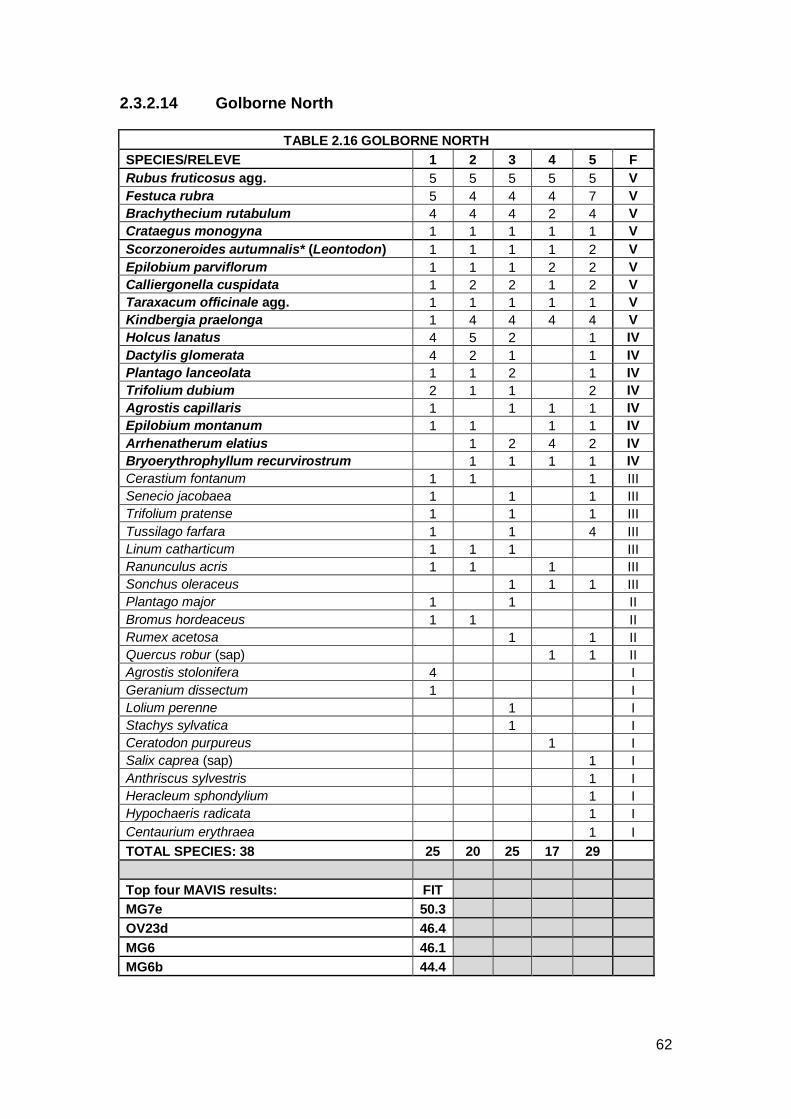
62
2.3.2.14 Golborne North
TABLE 2.16 GOLBORNE NORTH
SPECIES/RELEVE 1 2 3 4 5 F
Rubus fruticosus agg. 5 5 5 5 5 V
Festuca rubra 5 4 4 4 7 V
Brachythecium rutabulum 4 4 4 2 4 V
Crataegus monogyna 1 1 1 1 1 V
Scorzoneroides autumnalis* (Leontodon) 1 1 1 1 2 V
Epilobium parviflorum 1 1 1 2 2 V
Calliergonella cuspidata 1 2 2 1 2 V
Taraxacum officinale agg. 1 1 1 1 1 V
Kindbergia praelonga 1 4 4 4 4 V
Holcus lanatus 4 5 2 1 IV
Dactylis glomerata 4 2 1 1 IV
Plantago lanceolata 1 1 2 1 IV
Trifolium dubium 2 1 1 2 IV
Agrostis capillaris 1 1 1 1 IV
Epilobium montanum 1 1 1 1 IV
Arrhenatherum elatius 1 2 4 2 IV
Bryoerythrophyllum recurvirostrum 1 1 1 1 IV
Cerastium fontanum 1 1 1 III
Senecio jacobaea 1 1 1 III
Trifolium pratense 1 1 1 III
Tussilago farfara 1 1 4 III
Linum catharticum 1 1 1 III
Ranunculus acris 1 1 1 III
Sonchus oleraceus 1 1 1 III
Plantago major 1 1 II
Bromus hordeaceus 1 1 II
Rumex acetosa 1 1 II
Quercus robur (sap) 1 1 II
Agrostis stolonifera 4 I
Geranium dissectum 1 I
Lolium perenne 1 I
Stachys sylvatica 1 I
Ceratodon purpureus 1 I
Salix caprea (sap) 1 I
Anthriscus sylvestris 1 I
Heracleum sphondylium 1 I
Hypochaeris radicata 1 I
Centaurium erythraea 1 I
TOTAL SPECIES: 38 25 20 25 17 29
Top four MAVIS results: FIT MG7e 50.3 OV23d 46.4 MG6 46.1 MG6b 44.4

63
The Golborne North line was situated on relatively flat ground, surrounded by
farmland. The ballast was open towards the centre of the track with taller
vegetation growing close to the rails and Bramble encroaching across the
track. The vegetation cover was an average of 60%. A total of 38 species
were recorded including seventeen constants. Constants included
Scorzoneroides autumnalis, Holcus lanatus and Trifolium dubium along with
four species of bryophyte.
The CA shows the Golborne North plot close to W24 Rubus fruticosus-Holcus
lanatus underscrub and Rubus fruticosus agg. was the most abundant
species on the site. The top MAVIS result for Golborne North was MG7e
Lolium perenne leys Lolio–Plantaginetum sub-community. Considering that
Lolium perenne was not a constant species at Golborne North, MG7e seems
erroneous. MG6 Lolium perenne-Cynosurus cristatus grassland was the third
and fourth MAVIS result which can also be rejected due to the lack of
Cynosurus cristatus. A closer match to the existing NVC communities was
OV23d Lolium perenne–Dactylis glomerata community Arrhenatherum
elatius–Medicago lupulina sub-community which matched five constant
species; Dactylis glomerata, Plantago lanceolata, Taraxacum officinale agg.,
Arrhenatherum elatius and Holcus lanatus. OV23d was the second best fit in
MAVIS. However, this can be rejected because OV23 occurs on established
soils. In addition, the single specimen of Lolium perenne recorded at Golborne
North allows this community to be discounted. This community does have
affinities with MG1 Arrhenatherum elatius grassland but the grass species did
not record high cover values compared to Rubus fruticosus agg. so this

64
pushes the community away from MG1. Given the abundance of Rubus
fruticosus agg. in this community, and the presence of tree species as
saplings, Golborne North is classed as W24.

65
2.3.2.15 Golborne Sidings
TABLE 2.17 GOLBORNE SIDINGS
SPECIES/RELEVE 1 2 3 4 5 6 F
Festuca rubra 1 4 4 2 6 4 V
Anthriscus sylvestris 2 2 1 1 1 V
Dactylis glomerata 1 3 4 4 4 1 V
Taraxacum officinale agg. 1 1 1 1 1 V
Arrhenatherum elatius 1 1 6 6 6 4 V
Equisetum arvense 1 4 3 1 IV
Holcus lanatus 1 1 1 5 IV
Senecio viscosus 3 3 3 III
Plantago lanceolata 1 1 1 III
Agrostis capillaris 2 1 1 III
Rubus fruticosus agg. 1 1 1 III
Rumex acetosa 1 1 2 III
Vicia sativa 1 1 1 III
Sonchus asper 1 1 II
Barbarea vulgaris 1 2 II
Heracleum sphondylium 1 1 II
Agrostis stolonifera 1 1 II
Vicia cracca 1 1 II
Senecio vulgaris 1 I
Senecio jacobaea 1 I
Galium aparine 1 I
Ranunculus repens 1 I
Fragaria vesca 1 I
Urtica dioica 1 I
Rumex crispus 1 I
Epilobium hirsutum 1 I
Linaria vulgaris 1 I
Crataegus monogyna 1 I
TOTAL SPECIES: 28 10 15 9 13 15 12
Top four MAVIS results: FIT MG1a 55.5 MG9b 51.2 MG1b 51.0 MG1 48.6
The Golborne Sidings site is situated on a slight embankment surrounded by
arable land. The vegetation cover is low on the ballast with taller species such
as grasses and Umbellifers nearer to the rails. The community included many
ruderal species such as Linaria vulgaris and Senecio vulgaris. A total of 28
species were recorded from here which included seven constant species.
These included Festuca rubra, Equisetum arvense and Dactylis glomerata.

66
The CA shows Golborne Sidings as closest to MG1 Arrhenatherum elatius
grassland. The top MAVIS result for Golborne Sidings was to MG1a (Festuca
rubra sub-community). Given the dominance of grasses within the community,
MG1a is also the best fit when compared to the published tables. MG9b
Holcus lanatus–Deschampsia cespitosa grassland Arrhenatherum elatius
sub-community was the second match in MAVIS, however Deschampsia
cespitosa did not occur within this community and MG9 is a community of
damp soils. MG1 occurred as three out of the four MAVIS results and the
community did support four constant grass species and Anthriscus sylvestris
as a constant. It has been decided to place this community within MG1a.

67
2.3.2.16 Golborne South
TABLE 2.18 GOLBORNE SOUTH
SPECIES/RELEVE 1 2 3 4 5 F
Arrhenatherum elatius 8 7 6 7 6 V
Rubus fruticosus agg. 4 4 5 4 5 V
Bryoerythrophyllum recurvirostrum 4 4 4 1 1 V
Vicia sepium 2 4 1 1 IV
Festuca rubra 1 4 1 1 IV
Elytrigia repens 4 4 4 4 IV
Brachythecium rutabulum 4 4 4 III
Calliergonella cuspidata 4 2 2 III
Kindbergia praelongum 4 5 4 III
Equisetum arvense 1 6 4 III
Kindbergia praelonga 4 5 4 III
Ranunculus repens 1 1 II
Taraxacum officinale agg. 1 1 II
Epilobium montanum 1 1 II
Senecio jacobaea 1 1 II
Linaria vulgaris 1 I
Potentilla erecta 1 I
Sonchus oleraceus 1 I
Anthriscus sylvestris 1 I
Chamerion angustifolium 1 I
Epilobium parviflorum 1 I
Ceratodon purpureus 4 I
Salix caprea (sap) 1 I
Rumex crispus 1 I
Lolium perenne 1 I
Agrostis capillaris 2 I
Holcus lanatus 1 I
Centaurea nigra 1 I
Fraxinus excelsior (sap) 1 I
Galium aparine 1 I
Potentilla reptans 1 I
TOTAL SPECIES: 30 23 11 15 10 4
Top four MAVIS results: FIT MG1a 47.0 MG1b 42.6 MG1 41.0 MG1c 40.8
The Golborne South site was situated in a shallow cutting surrounded by
farmland. The slopes of the cutting were dominated by scrub. The community
was dominated by Arrhenatherum elatius with Bramble encroaching across
the track. Bryophytes were abundant in addition to ruderal species. The

68
vegetation cover averaged 90% over the granite ballast. A total of 30 species
were recorded with six constants. These included Vicia sepium, Elytrigia
repens and Bryoerythrophyllum recurvirostrum.
The CA shows the Golborne South plot very close to W24 Rubus fruticosus–
Holcus lanatus underscrub. By comparison MG1 was suggested in all four
MAVIS results. However, the presence of bryophytes and tree saplings within
the community along with ruderal species, is more suggestive of W24b
(Arrhenatherum elatius–Heracleum sphondylium sub-community) as is the
presence of Rubus fruticosus agg. and Arrhenatherum elatius as constants.
The Golborne South community is classed as W24b.

69
2.3.2.17 Histon to St. Ives East
TABLE 2.19 HISTON TO ST. IVES EAST
SPECIES/RELEVE 1 2 3 F
Senecio viscosus 4 2 2 V
Scorzoneroides autumnalis* 2 2 2 V
Lamium album 4 2 2 V
Arenaria serpyllifolia ssp. leptoclados 2 2 2 V
Helminthotheca echioides* (Picris echioides) 1 1 1 V
Rubus fruticosus agg. 5 5 IV
Achillea millefolium 4 4 IV
Stellaria media 1 1 IV
Urtica dioica 1 1 IV
Knautia arvensis 4 4 IV
Lamium purpureum 4 2 IV
Dipsacus fullonum 2 4 IV
Epilobium montanum 1 1 IV
Crataegus monogyna (sap) 1 1 IV
Geum urbanum 4 4 IV
Glechoma hederacea 2 2 IV
Cerastium fontanum 1 1 IV
Dactylis glomerata 4 2 IV
Cirsium arvense 1 1 IV
Chamerion angustifolium 2 4 IV
Rumex acetosa 1 1 IV
Chenopodium polyspermum 2 II
Senecio jacobaea 1 II
Veronica arvensis 1 II
Myosotis arvensis 2 II
Viola arvensis 2 II
Potentilla reptans 4 II
Taraxacum officinale agg. 1 II
Lactuca serriola 4 II
Prunella vulgaris 1 II
Geranium molle 2 II
Rosa pimpinellifolia 2 II
Hieraceum sp. 1 II
Poa annua 1 II
Veronica chamaedrys 1 II
Convolvulus arvensis 2 II
Solanum dulcamara 4 II
Berberis sp. 4 II
Fraxinus excelsior (sap) 1 II
Stachys sylvatica 1 II
Centaurea nigra 4 II
Hypericum perforatum 2 II
Tanacetum vulgare 4 II
Holcus lanatus 4 II
Conyza canadensis 4 II
Artemisia absinthium 4 II
Sedum acre 2 II

70
SPECIES/RELEVE 1 2 3 F
Pastinaca sativa 4 II
TOTAL SPECIES: 48 24 30 20
Top four MAVIS results: FIT MG1 31.0 MG1d 30.3 MG1a 27.7 W24a 27.0
The Histon to St. Ives East site was situated on a slight embankment,
surrounded by buildings, gardens and disused land. The community was
species-rich with low-growing ruderal species dominating and Bramble
encroaching across the rails. The vegetation coverage over the ballast was on
average 75%, with most plants occurring near to the rails with open ballast in
the centre. A total of 48 species were recorded here, including 21 constant
species. These included Glechoma hederacea, Knautia arvensis, Dipsacus
fullonum and Scorzoneroides autumnalis.
The CA shows the Histon to St. Ives East plot as distant from any of the four
NVC community plots. The top three MAVIS results for Histon to St. Ives East
were MG1 Arrhenatherum elatius grasslands. However the combination of
ruderal constants and absence of grass constants (indeed Arrhenatherum
elatius is absent here) means that MG1 is an inappropriate allocation. A sub-
community of the closest community on the CA plot (OV23d Lolium perenne–
Dactylis glomerata community Arrhenatherum elatius–Medicago lupulina sub-
community is a slightly better match due to the presence of annual species
and the constants Achillea millefolium and Dactylis glomerata. However,
OV23 is typical of previously managed sites with well established soil. In
addition, Lolium perenne is absent. Hence OV23 is also an inappropriate

71
designation. W24a Rubus fruticosus-Holcus lanatus underscrub Cirsium
arvense-Cirsium vulgare sub-community was the fourth MAVIS result.
However, the community does not have the physiognomy of scrub, and given
the number of ruderal species, W24 can be rejected. Due to the species
assemblage at this site, and the location on the CA, this community
does not match any existing NVC community.

72
2.3.2.18 Histon to St. Ives West
TABLE 2.20 HISTON TO ST. IVES WEST
SPECIES/RELEVE 1 2 3 4 5 F
Rubus fruticosus agg. 5 2 4 4 4 V
Medicago lupulina 5 8 4 8 5 V
Achillea millefolium 4 4 4 4 IV
Lolium perenne 4 4 4 4 IV
Centaurea nigra 2 4 2 4 IV
Leucanthemum vulgare 4 2 4 2 IV
Pilosella officinarum 4 4 4 4 IV
Crataegus monogyna (sap) 2 4 2 2 IV
Cerastium glomeratum 1 1 1 2 IV
Scorzoneroides autumnalis* 3 1 2 4 IV
Geranium molle 4 4 1 III
Hypericum perforatum 4 4 1 III
Galium verum 2 5 2 III
Prunella vulgaris 1 1 1 III
Sonchus asper 4 2 2 III
Rumex acetosa 2 1 4 III
Senecio jacobaea 4 2 4 III
Veronica chamaedrys 1 2 4 III
Pastinaca sativa 4 4 4 III
Knautia arvensis 4 4 2 III
Myosotis arvensis 2 2 1 III
Plantago lanceolata 4 4 4 III
Chamerion angustifolium 2 1 2 III
Brachypodium sylvaticum 4 5 II
Verbascum thapsus 4 4 II
Festuca rubra 4 1 II
Dactylis glomerata 1 4 II
Geranium dissectum 2 1 II
Bellis perennis 1 1 II
Holcus lanatus 4 4 II
Taraxacum officinale agg. 2 2 II
Viola canina agg. 1 4 II
Rosa pimpinellifolia 3 1 II
Urtica dioica 1 2 II
Epilobium sp. 2 1 II
Arenaria serpyllifolia ssp. leptoclados 4 2 II
Arrhenatherum elatius 4 6 II
Daucus carota 1 4 II
Senecio viscosus 4 I
Agrostemma githago 2 I
Conyza canadensis 4 I
Solanum dulcamara 2 I
Betula sp. (seedling) 1 I
Stachys sylvatica 2 I
Stellaria media 2 I
Arabidopsis thaliana 1 I
Lamium album 2 I
Ceratodon purpureus 2 I
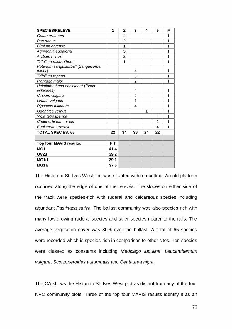
73
SPECIES/RELEVE 1 2 3 4 5 F
Geum urbanum 4 I
Poa annua 2 I
Cirsium arvense 1 I
Agrimonia eupatoria 5 I
Arctium minus 2 I
Trifolium micranthum 1 I Poterium sanguisorba* (Sanguisorba minor) 4 I
Trifolium repens 3 I
Plantago major 2 I Helminthotheca echioides* (Picris echioides) 4 I
Cirsium vulgare 2 I
Linaria vulgaris 1 I
Dipsacus fullonum 4 I
Odontites vernus 1 I
Vicia tetrasperma 4 I
Chaenorhinum minus 1 I
Equisetum arvense 4 I
TOTAL SPECIES: 65 22 34 36 24 22
Top four MAVIS results: FIT MG1 41.4 OV23 39.2 MG1d 39.1 MG1a 37.5
The Histon to St. Ives West line was situated within a cutting. An old platform
occurred along the edge of one of the relevés. The slopes on either side of
the track were species-rich with ruderal and calcareous species including
abundant Pastinaca sativa. The ballast community was also species-rich with
many low-growing ruderal species and taller species nearer to the rails. The
average vegetation cover was 80% over the ballast. A total of 65 species
were recorded which is species-rich in comparison to other sites. Ten species
were classed as constants including Medicago lupulina, Leucanthemum
vulgare, Scorzoneroides autumnalis and Centaurea nigra.
The CA shows the Histon to St. Ives West plot as distant from any of the four
NVC community plots. Three of the top four MAVIS results identify it as an

74
MG1 Arrhenatherum elatius grassland. However, Arrhenatherum elatius and
Holcus lanatus were infrequently recorded at this site and the community
cannot be described as a grassland. Comparing the NVC tables, OV23d
Lolium perenne–Dactylis glomerata community Arrhenatherum elatius–
Medicago lupulina sub-community appears to be a slightly better fit. OV23d
includes Lolium perenne, Medicago lupulina and Achillea millefolium as
constant species which Histon to St. Ives West matches. OV23 was the
second result from MAVIS for this community but OV23 is rejected due to the
lack of established soil which typifies OV23 and the combination of ruderal
and calcareous species present. Due to the species-rich assemblage, with
some calcareous species and many ruderal species, and given the
location of the plot on CA, this community cannot be placed within an
existing NVC classification.
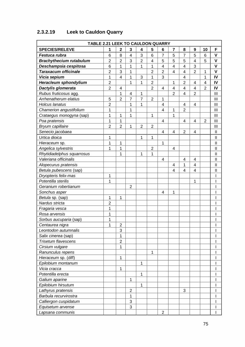
75
2.3.2.19 Leek to Cauldon Quarry
TABLE 2.21 LEEK TO CAULDON QUARRY
SPECIES/RELEVE 1 2 3 4 5 6 7 8 9 10 F
Festuca rubra 6 8 4 3 6 7 5 7 5 6 V
Brachythecium rutabulum 2 2 3 2 4 5 5 5 4 5 V
Deschampsia cespitosa 6 1 1 1 1 4 4 4 3 V
Taraxacum officinale 2 3 1 2 2 4 4 2 1 V
Vicia sepium 1 4 1 3 1 3 4 1 IV
Heracleum sphondylium 2 1 1 2 1 2 4 4 IV
Dactylis glomerata 2 4 2 4 4 4 4 2 IV
Rubus fruticosus agg. 1 4 1 2 4 2 III
Arrhenatherum elatius 5 2 7 7 2 1 III
Holcus lanatus 2 1 1 4 4 4 III
Chamerion angustifolium 1 1 4 1 2 III
Crataegus monogyna (sap) 1 1 1 1 1 III
Poa pratensis 1 1 4 4 4 2 III
Bryum capillaire 2 2 1 2 2 III
Senecio jacobaea 4 4 2 4 II
Urtica dioica 1 1 1 II
Hieraceum sp. 1 1 1 II
Angelica sylvestris 1 1 2 4 II
Rhytidiadelphus squarrosus 1 1 1 II
Valeriana officinalis 4 4 4 II
Alopecurus pratensis 4 1 4 II
Betula pubescens (sap) 4 4 4 II
Dryopteris felix-mas 1 I
Potentilla sterilis 1 1 I
Geranium robertianum 2 I
Sonchus asper 4 1 I
Betula sp. (sap) 1 1 I
Nardus stricta 2 I
Fragaria vesca 1 I
Rosa arvensis 1 I
Sorbus aucuparia (sap) 1 I
Centaurea nigra 1 2 I
Leontodon autumnalis 3 I
Salix cinerea (sap) 1 I
Trisetum flavescens 2 I
Cirsium vulgare 1 I
Ranunculus repens 1 I
Hieraceum sp. (diff) 1 I
Epilobium montanum 1 I
Vicia cracca 1 I
Potentilla erecta 1 I
Galium aparine 1 I
Epilobium hirsutum 1 I
Lathyrus pratensis 2 3 I
Barbula recurvirostra 1 I
Calliergon cuspidatum 3 I
Equisetum arvense 3 I
Lapsana communis 2 I

76
SPECIES/RELEVE 1 2 3 4 5 6 7 8 9 10 F
Primula vulgaris 1 I
Ranunculus acris 4 I
Ilex aquifolium 1 I
Corylus avellana 1 I Schedonorus pratensis* (Festuca pratensis) 4 I
Festuca ovina 2 I
Epilobium sp. 2 I
Geum urbanum 2 I
TOTAL SPECIES: 56 24 22 18 14 14 17 15 16 19 7
Top four MAVIS results: FIT MG1a 46.4 W24b 46.4 MG1 45.1 W24 44.4
The Leek to Cauldon Quarry line was situated on an exposed embankment.
The community comprised tall tufted grasses growing close to the rails with
low-growing species, including some acidic grassland species, occurring
sporadically across the ballast. The surrounding land was permanent pasture,
grazed by livestock which had no access to the railway line. A total of 56
species were recorded from this site with a total of seven constant species.
These included Vicia sepium, Heracleum sphondylium, Festuca rubra and the
moss Brachythecium rutabulum. The latter two species achieved high Domin
scores, the rest of the constant species had low cover values. The average
ballast cover was 70%.
The CA shows the Leek to Cauldon Quarry plot as equidistant between MG1
Arrhenatherum elatius grassland and W24 Rubus fruticosus–Holcus lanatus
underscrub. The top MAVIS result for the Leek to Cauldon line was to both
MG1a (Festuca rubra sub-community) and W24b (Arrhenatherum elatius-
Heracleum sphondylium sub-community). The Leek to Cauldon Quarry line

77
did not support Arrhenatherum elatius as a constant species, neither were
Rubus fruticosus agg. nor Holcus lanatus recorded as constants. This
community has affinities with both MG1 (given the presence of tall grass
species and Umbellifers) and W24 (given the Bramble and the presence
of tree species as saplings) but the community cannot be placed within
any existing NVC community.

78
2.3.2.20 Leek to Cauldon Quarry Wooded
TABLE 2.22 LEEK TO CAULDON QUARRY WOODED
SPECIES/RELEVE 1 2 3 F
Vicia sepium 2 2 4 V
Rubus fruticosus agg. 4 3 4 V
Brachythecium rutabulum 6 5 IV
Dactylis glomerata 7 4 IV
Chamerion angustifolium 4 3 IV
Senecio jacobaea 2 3 IV
Dryopteris felix-mas 4 4 IV
Geranium robertianum 1 1 IV
Sonchus asper 2 3 IV
Betula pubescens 4 1 IV
Agrostis capillaris 4 4 IV
Festuca rubra 4 I
Heracleum sphondylium 1 I
Taraxacum officinale agg. 2 I
Arrhenatherum elatius 2 I
Holcus lanatus 5 I
Crataegus monogyna 1 I
Angelica sylvestris 4 I
Potentilla sterilis 1 I
Sorbus aucuparia 2 I
Scorzoneroides autumnalis 4 I
Ranunculus repens 4 I
Galium aparine 1 I
Epilobium sp. 2 I
Geum urbanum 4 I
Epilobium parviflorum 2 I
Prunella vulgaris 1 I
Scrophularia nodosa 2 I
Salix sp. 1 I
Poa annua 4 I
Medicago lupulina 1 I
TOTAL SPECIES: 31 10 13 21
Top four MAVIS results: FIT W24 36.8 W24b 35.6 W24a 35.1 MG1a 33.0
The Leek to Cauldon Quarry Wooded site was situated on a low embankment
with dense woodland either side of the track. In parts, the vegetation covered
most of the ballast whereas in other places, the ballast was relatively open.
The community comprised isolated grass species with Umbellifers and tree

79
saplings and some ruderal species. A total of 31 species were recorded here
with eleven constant species, most of which were recorded with low Domin
scores. Constants included Vicia sepium, Dryopteris felix-mas, Sonchus asper
and Chamerion angustifolium.
The CA shows the Leek to Cauldon Quarry Wooded plot as closest to W24
Rubus fruticosus–Holcus lanatus underscrub albeit some distance from the
W24 plot. The top MAVIS result for this small section of shaded line was to
W24 Rubus fruticosus–Holcus lanatus underscrub with W24b (Arrhenatherum
elatius–Heracleum sphondylium sub-community) the second best match.
Comparing the published NVC tables, W24b fits best due to the rank grasses
(e.g. Dactylis glomerata) and Umbellifers (e.g. Heracleum sphondylium) which
were recorded frequently. MG1a Arrhenatherum elatius grassland Festuca
rubra sub-community, the fourth MAVIS result, can be rejected due to the very
low cover of Arrhenatherum elatius. Given the Bramble and tree saplings
present on the site and the location of the CA plot, this community is
classed as having affinities to W24 but is difficult to place clearly within
an existing NVC community.

80
2.3.2.21 Leek to Stoke
TABLE 2.23 LEEK TO STOKE
SPECIES/RELEVE 1 2 3 4 5 6 F
Epilobium sp. 4 4 4 2 3 4 V
Taraxacum officinale agg. 4 4 4 2 4 4 V
Senecio jacobaea 4 4 4 1 4 V
Festuca rubra 6 6 6 5 7 6 V
Chamerion angustifolium 2 4 4 4 2 4 V
Sonchus asper 2 4 2 2 2 V
Arabidopsis thaliana 4 2 2 4 1 1 V
Angelica sylvestris 4 4 1 2 2 V
Brachythecium rutabulum 4 5 4 4 4 V
Rubus idaeus 4 2 2 1 1 V
Holcus lanatus 5 4 4 4 4 V
Dactylis glomerata 1 4 4 4 IV
Rhytidiadelphus squarrosus 4 4 4 4 IV
Hieraceum sp. 1 4 1 1 IV
Pilosella officinarum 1 4 4 4 IV
Hypochaeris radicata 4 4 2 4 IV
Rubus fruticosus agg. 1 2 1 III
Linaria vulgaris 4 2 1 III
Plantago lanceolata 4 1 1 III
Potentilla sterilis 4 2 3 III
Bellis perennis 4 4 1 III
Ranunculus acris 1 2 2 III
Solanum dulcamara 4 1 1 III
Barbula sp. 4 3 5 III
Vicia sepium 2 4 4 III
Poa annua 5 5 II
Trifolium repens 4 1 II
Cirsium vulgare 1 1 II
Lolium perenne 4 4 II
Cerastium fontanum 1 2 II
Vicia sativa 4 4 II
Rosa arvensis 2 4 II
Valeriana officinalis 1 3 II
Veronica arvensis 1 4 II
Scrophularia nodosa 2 2 II
Lapsana communis 1 1 II
Heracleum sphondylium 1 1 II
Cirsium arvense 1 4 II
Bryum sp. 4 4 II
Hypnum cupressiforme 2 4 II
Lathyrus pratensis 4 4 II
Alopecurus pratensis 2 5 II
Crataegus monogyna (sap) 1 1 II
Leucanthemum vulgare 4 I
Hieraceum sp. 4 I
Vicia cracca 5 I
Plantago major 4 I
Urtica dioica 1 I

81
SPECIES/RELEVE 1 2 3 4 5 6 F
Salix sp. (sap) 1 I
Vicia hirsuta 4 I
Racomitrium sp. 2 I Amblystegium serpens var. serpens 2 I
Arenaria serpyllifolia 1 I
Veronica chamaedrys 1 I
Filipendula ulmaria 2 I
Kindbergia praelongum 1 I
Lophocolea sp. 4 I
Calliergon cuspidatum 4 I
Viola canina agg. 2 I
Campylopus introflexus 2 I
Polytrichum commune 3 I
Digitalis purpurea 4 I
Luzula multiflorum 4 I
Deschampsia cespitosa 4 I
Cirsium palustre 4 I
Epilobium parviflorum 4 I
Trifolium campestre 1 I
Anthriscus sylvestris 4 I
Cardamine hirsuta 2 I
Agrostis capillaris 4 I
Phleum pratense 4 I
Dipsacus fullonum 4 I
Arrhenatherum elatius 4 I
Galium aparine 1 I
TOTAL SPECIES: 74 32 36 27 28 26 25
Top four MAVIS results: FIT MG1a 37.6 MG1 37.4 MG6a 36.9 MG5 36.8
The Leek to Stoke line was situated on relatively flat ground with a slight
decline on the south side leading down to the Caldon Canal. The vegetation
covering was on average 75% on the ballast with taller vegetation occurring
nearer to the rails and Raspberry encroaching across the rails. A total of 74
species were recorded with sixteen constant species. These are
predominantly ruderal species and include Arabidopsis thaliana, Sonchus
asper, Angelica sylvestris and Pilosella officinarum. These all exhibited low
ground cover values. Twelve species of bryophyte were also recorded here.

82
The CA shows the Leek to Stoke plot as close to both MG1 Arrhenatherum
elatius grassland and W24 Rubus fruticosus-Holcus lanatus underscrub. The
top MAVIS result for the Leek to Stoke sample was MG1a (Festuca rubra sub-
community). Only Festuca rubra matches the constants in the MG1
community (Arrhenatherum elatius is only present on one relevé). Likewise
the low cover of Rubus fruticosus agg. eliminates W24 as the community at
this site. MG6a Lolium perenne-Cynosurus cristatus grassland typical sub-
community was the third MAVIS result but the Leek to Stoke community did
not support Cynosurus cristatus and Lolium perenne was not recorded as
constant. MG5 Cynosurus cristatus-Centaurea nigra grassland was the fourth
MAVIS result. Neither of these title species were recorded at Leek to Stoke so
this community can be rejected. The combination of constant species in
the Leek to Stoke community mean that it does not fit into any existing
NVC community. The CA has to be disregarded in this instance.
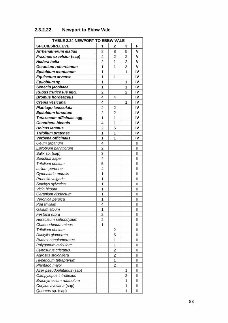
83
2.3.2.22 Newport to Ebbw Vale
TABLE 2.24 NEWPORT TO EBBW VALE
SPECIES/RELEVE 1 2 3 F
Arrhenatherum elatius 8 8 5 V
Fraxinus excelsior (sap) 4 2 2 V
Hedera helix 2 1 2 V
Geranium robertianum 1 1 3 V
Epilobium montanum 1 1 IV
Equisetum arvense 1 1 IV
Epilobium sp. 1 1 IV
Senecio jacobaea 1 1 IV
Rubus fruticosus agg. 2 2 IV
Bromus hordeaceus 4 4 IV
Crepis vesicaria 4 1 IV
Plantago lanceolata 2 2 IV
Epilobium hirsutum 2 2 IV
Taraxacum officinale agg. 1 1 IV
Oenothera biennis 4 1 IV
Holcus lanatus 2 5 IV
Trifolium pratense 1 1 IV
Verbena officinalis 1 1 IV
Geum urbanum 4 II
Epilobium parviflorum 2 II
Salix sp. (sap) 3 II
Sonchus asper 4 II
Trifolium dubium 5 II
Lolium perenne 4 II
Cymbalaria muralis 1 II
Prunella vulgaris 1 II
Stachys sylvatica 1 II
Vicia hirsuta 1 II
Geranium dissectum 1 II
Veronica persica 1 II
Poa trivialis 4 II
Galium album 1 II
Festuca rubra 2 II
Heracleum sphondylium 2 II
Chaenorhinum minus 1 II
Trifolium dubium 2 II
Dactylis glomerata 5 II
Rumex conglomeratus 1 II
Polygonum aviculare 1 II
Cynosurus cristatus 2 II
Agrostis stolonifera 2 II
Hypericum tetrapterum 1 II
Plantago major 2 II
Acer pseudoplatanus (sap) 1 II
Campylopus introflexus 2 II
Brachythecium rutabulum 1 II
Corylus avellana (sap) 1 II
Quercus sp. (sap) 1 II

84
SPECIES/RELEVE 1 2 3 F
Buddleja davidii 1 II
Asplenium adiantum-nigrum 1 II
Chamerion angustifolium 2 II
Betula pendula (sap) 1 II
TOTAL SPECIES: 52 35 21 18
Top four MAVIS results: FIT OV23 37.2 W24 33.6 OV23c 33.1 MG1a 32.9
The Newport to Ebbw Vale site was situated in a shallow cutting. To the north
lay ex-industrial land covered with ruderal vegetation. To the south lay an A
road and housing. The community comprised tall Arrhenatherum elatius
growing close to the rails with scattered tree saplings and many ruderal
species. The vegetation cover was, on average, 75% on the ballast. A total of
52 species were recorded here with eighteen of these being constants.
Constant species included Verbena officinalis, Fraxinus excelsior (sapling),
Senecio jacobaea and Oenothera biennis.
The top MAVIS result for Newport to Ebbw Vale was OV23 Lolium perenne–
Dactylis glomerata community. This can be rejected due to the very low cover
of both these species at the site. The second best fit from MAVIS was W24
Rubus fruticosus–Holcus lanatus underscrub. The Newport to Ebbw Vale
community included Fraxinus excelsior saplings and Hedera helix as well as
W24 constants Rubus fruticosus agg., Holcus lanatus, Taraxacum officinale
agg. and Arrhenatherum elatius. However, Rubus fruticosus agg. and Holcus
lanatus were recorded with very low cover values. MG1a Arrhenatherum
elatius grassland Festuca rubra sub-community was the fourth MAVIS result.

85
This can be explained by the constants Arrhenatherum elatius and Holcus
lanatus. And the former species did have high cover values. However, the
combination of ruderal species and tree saplings are not characteristic of
MG1. The CA plot shows the Newport to Ebbw Vale plot as equidistant from
W24 and MG1 albeit some distance from either. This community is
therefore classed as having affinities to MG1 and W24 but cannot be
placed exactly into either.

86
2.3.2.23 Oswestry North Embankment
TABLE 2.25 OSWESTRY NORTH EMBANKMENT
SPECIES/RELEVE 1 2 3 4 5 F
Arrhenatherum elatius 4 6 5 5 7 V
Buddleja davidii 7 5 6 5 7 V
Rubus fruticosus agg. 1 2 2 2 4 V
Epilobium montanum 1 1 1 1 IV
Geum urbanum 1 1 1 1 IV
Holcus lanatus 2 4 1 III
Lolium perenne 1 1 4 III
Trifolium dubium 2 1 1 III
Rhytidiadelphus squarrosus 2 1 1 III
Betula pendula (sap) 2 4 4 III
Salix caprea (sap) 4 7 5 III
Leontodon hispidus 2 1 II
Senecio jacobaea 1 1 II
Tragopogon pratensis 1 1 II
Convolvulus arvensis 1 1 II
Chamerion angustifolium 1 4 II
Calliergonella cuspidata 1 1 II
Sagina procumbens 1 1 II
Festuca rubra 1 1 II
Poa annua 1 1 II
Dipsacus fullonum 1 1 II
Crataegus monogyna (sap) 1 1 II
Vicia hirsuta 4 I
Hedera helix 1 I
Hypochaeris radicata 1 I
Vulpia bromoides 4 I
Hypericum sp. 1 I
Ceratodon purpureus 2 I
Agrostis capillaris 1 I
Geranium dissectum 1 I
Prunella vulgaris 1 I
Acer pseudoplatanus (sap) 1 I
Trifolium campestre 1 I
Epilobium parviflorum 1 I
Plantago lanceolata 1 I
Lapsana communis 1 I
Poa trivialis 1 I
Urtica dioica 1 I
Galium album 1 I
Geranium molle 1 I
Mercurialis perennis 1 I
Plantago major 1 I
Poa pratensis 1 I
Dactylis glomerata 1 I
Fragaria vesca 1 I

87
TOTAL SPECIES: 45 34 24 7 10 11
Top four MAVIS results: FIT OV23 40.4 W24 39.3 MG1a 38.0 MG1 36.1
The Oswestry North Embankment site was on a viaduct. On the edge of the
track was tall scrub. Tall vegetation, mainly Buddleja and Arrhenatherum
elatius, dominated the track with Bramble beneath and the vegetation cover
averaged 60%. This was a relatively species-rich railway line. A total of 45
species were recorded including five constants. These included Buddleja
davidii and Geum urbanum though no existing NVC community includes these
species as constants.
The top MAVIS result for Oswestry North Embankment was OV23 Lolium
perenne–Dactylis glomerata community. However, OV23 matches only
Arrhenatherum elatius as a constant species and ecologically does not fit the
community. MG1 Arrhenatherum elatius grassland came out as third and
fourth MAVIS results. Despite Arrhenatherum elatius being constant in the
community, MG1 can be rejected due to the lack of grassland physiognomy
and the presence of ruderal and scrub species. The scrub species are
characteristic of W24 and this is supported by the position on the CA plot,
although the presence of Buddleja and ruderals as constants are untypical of
the community. This community is classed as W24 with Buddleja.

88
2.3.2.24 Runcorn Docks
TABLE 2.26 RUNCORN DOCKS
SPECIES/RELEVE 1 2 3 4 5 6 7 8 9 10 F
Vulpia bromoides 6 7 6 7 6 5 5 4 4 2 V
Galium aparine 2 2 2 1 2 1 1 1 1 V
Senecio jacobaea 2 1 1 1 1 1 1 1 1 V
Arrhenatherum elatius 5 4 4 4 4 5 5 4 5 5 V
Sonchus asper 1 2 2 4 1 1 1 2 2 1 V
Taraxacum officinale agg. 1 2 1 1 1 1 1 1 1 V
Anthriscus sylvestris 1 2 1 2 2 1 1 2 2 V
Holcus lanatus 2 4 2 2 1 2 2 IV
Veronica arvensis 1 1 1 1 1 1 1 IV
Cerastium fontanum 1 1 1 1 1 1 1 IV
Epilobium montanum 1 1 1 1 1 1 1 IV
Pimpinella saxifraga 2 2 1 1 2 1 2 IV
Helminthotheca echioides* 1 2 4 1 1 2 1 IV
Hypochaeris radicata 2 3 2 2 1 1 III
Heracleum sphondylium 2 1 1 1 1 1 III
Centaurium erythraea 1 1 1 1 1 III
Linum catharticum 1 1 1 1 1 1 III
Dactylis glomerata 2 1 2 2 2 1 III
Senecio viscosus 1 1 1 1 1 III
Hieraceum sp. 1 1 1 1 2 1 III
Rubus fruticosus agg. 1 1 2 1 II
Conyza canadensis 2 1 4 1 II
Epilobium parviflorum 1 1 1 1 II
Brachythecium rutabulum 2 1 4 II
Rumex crispus 4 2 1 2 II
Verbascum thapsus 1 2 1 1 II
Artemisia vulgaris 1 2 1 II
Solanum dulcamara 1 1 1 II
Cirsium arvense 1 2 2 II
Leontodon hispidus 1 1 1 II
Crepis vesicaria 1 1 1 1 II
Hypericum perforatum 1 2 1 II
Medicago lupulina 1 1 1 1 II
Equisetum arvense 1 I
Epilobium palustre 1 1 I
Cerastium glomeratum 1 1 I
Senecio jacobaea 1 I
Reseda luteola 1 I
Rumex acetosa 1 I
Deschampsia cespitosa 2 I
Cirsium vulgaris 1 I
Geranium robertianum 1 I
Anisantha sterilis 2 I
Tragopogon pratensis 3 1 I
Vicia cracca 1 1 I
Stachys sylvatica 1 2 I
Festuca rubra 1 I
Urtica dioica 1 I

89
SPECIES/RELEVE 1 2 3 4 5 6 7 8 9 10 F
Blackstonia perfoliata 1 I
Chamerion angustifolium 1 4 I
Scrophularia nodosa 2 I
Sambucus nigra (sap) 4 I
Plantago lanceolata 1 I
TOTAL SPECIES: 52 28 30 26 24 22 25 19 20 12 13
Top four MAVIS results: FIT MG1 39.6 OV23 39.2 W24 38.7 MG1b 37.9
The Runcorn Docks site was situated on a tall embankment between
industrial buildings, to the west lay industrial buildings with a dual carriageway
to the east. The vegetation comprised tufted grasses and low-growing
herbaceous species over granite ballast. Vegetation cover averaged 50%. A
total of 52 species were recorded, including thirteen constant species. These
included Veronica arvensis, Pimpinella saxifraga and Cerastium fontanum.
The CA shows the Runcorn Docks plot as equidistant from OV23 Lolium
perenne–Dactylis glomerata community and MG1 Arrhenatherum elatius
grassland. The top MAVIS result for Runcorn Docks was MG1. This
corresponds to several elements of the community; the constant
Arrhenatherum elatius with the tall Umbellifers Anthriscus sylvestris and
Heracleum sphondylium plus Dactylis glomerata frequent. However the
community has a significant ruderal component which is not characteristic of
MG1. OV23 can be rejected due to the lack of Lolium perenne and Dactylis
glomerata from the constants. W24 Rubus fruticosus–Holcus lanatus
underscrub (the third MAVIS result) can be rejected due to the low cover of

90
Rubus fruticosus agg. The Runcorn Docks site is therefore classed as
having affinities to MG1 but with a ruderal element.

91
2.3.2.25 St. Helens Acid Works
TABLE 2.27 ST. HELENS ACID WORKS
SPECIES/RELEVE 1 2 3 4 5 F
Arrhenatherum elatius 7 7 7 5 1 V
Rubus fruticosus agg. 1 4 1 3 1 V
Festuca ovina 1 1 1 4 1 V
Holcus lanatus 1 1 1 1 1 V
Agrostis stolonifera 1 1 1 8 4 V
Stachys sylvatica 1 1 1 1 IV
Salix cinerea (sap) 1 1 4 1 IV
Sonchus asper 1 1 1 1 IV
Taraxacum officinale agg. 1 1 1 1 IV
Eupatorium cannabinum 1 3 7 1 IV
Senecio squalidus 1 1 1 III
Epilobium parviflorum 2 1 1 III
Calystegia sepium 1 2 1 III
Epilobium hirsutum 4 1 2 III
Crataegus monogyna 1 1 II
Acer pseudoplatanus (sap) 1 1 II
Vicia cracca 1 1 II
Chamerion angustifolium 1 1 II
Cerastium fontanum 1 1 II
Salix sp. (sap) 1 1 II
Rumex crispus 1 1 II
Epilobium sp. 1 I
Plantago lanceolata 1 I
Medicago lupulina 4 I
Sagina procumbens 1 I
Poa annua 1 I
Geranium robertianum 1 I
Linaria vulgaris 1 I
Prunus sp. (sap) 1 I
Tussilago farfara 1 I
Hypochaeris radicata 1 I
Lotus corniculatus 4 I
Solidago canadensis 1 I
Rosa canina 1 I
Hieraceum sp. 1 I
TOTAL SPECIES: 35 18 21 15 19 12
Top four MAVIS results: FIT OV23d 32.5 OV23 29.9 OV23c 27.8 OV22a 27.7
St. Helens Acid Works is situated in a flat area of land, sandwiched between
factories and the derelict acid works site. Tall, ruderal vegetation exists on the

92
land next to the track. The community was dominated by tall Eupatorium
cannabinum and Arrhenatherum elatius growing near to the rails with ruderal
species scattered on the ballast. Throughout the sample, the cover of the
vegetation differed over the ballast. In places, the cover was sparse, in others
the cover reached 95%. A total of 35 species were recorded here including
ten constant species. These included Eupatorium cannabinum, Agrostis
stolonifera and Festuca ovina. Eupatorium cannabinum is not identified as a
constant in any NVC communities.
The CA shows the St. Helens Acid Works plot as closest to MG1
Arrhenatherum elatius grassland. The MAVIS results almost all identify OV23
Lolium perenne–Dactylis glomerata communities as the most similar. This
result can be rejected due to the lack of both Lolium perenne and Dactylis
glomerata at the site. This railway community has OV22a Poa annua-
Taraxacum officinale community Senecio vulgaris sub-community was the
fourth MAVIS result. This can be rejected due to the absence of Poa annua.
Comparing MG1 and W24, the community supports more Arrhenatherum
elatius than Rubus fruticosus agg. but does support tree and scrub species as
saplings. This community is classed as having affinities with MG1 and
W24 but is an open community with constants that do not match any
sub-communities of either MG1 or W24.

93
2.3.2.26 St. Helens Canal North
TABLE 2.28 ST. HELENS CANAL NORTH
SPECIES/RELEVE 1 2 3 4 5 F
Senecio jacobaea 2 1 1 4 1 V
Taraxacum officinale agg. 1 1 1 1 1 V
Eupatorium cannabinum 5 5 5 4 4 V
Galium aparine 1 2 1 1 1 V
Epilobium parviflorum 1 1 2 1 1 V
Arrhenatherum elatius 2 2 1 1 4 V
Vulpia bromoides 4 5 4 4 2 V
Trifolium dubium 4 4 4 2 2 V
Holcus lanatus 1 2 4 4 2 V
Brachythecium rutabulum 1 4 1 4 1 V
Barbula convoluta 2 1 1 2 1 V
Festuca rubra 1 1 1 1 2 V
Agrostis stolonifera 4 4 2 2 IV
Linum catharticum 4 2 1 1 IV
Buddleja davidii 1 1 1 4 IV
Myosotis discolor 1 1 1 1 IV
Betula pubescens (sap) 1 2 1 1 IV
Sonchus oleraceus 1 1 1 1 IV
Chamerion angustifolium 1 4 2 2 IV
Poa annua 1 1 1 1 IV
Agrostis capillaris 2 4 1 1 IV
Euphrasia officinalis 2 4 1 2 IV
Epilobium montanum 1 1 2 1 IV
Bryum argenteum 1 1 4 1 IV
Pastanica sativa 1 1 2 III
Epilobium palustre 1 1 1 III
Plantago major 1 1 1 III
Betula pendula (sap) 4 4 1 III
Salix caprea (sap) 4 2 2 III
Centaurium erythraea 1 1 1 III
Alnus glutinosa (sap) 2 4 2 III
Sagina procumbens 1 1 1 III
Centaurea nigra 1 1 2 III
Lolium perenne 1 1 II
Dactylis glomerata 1 2 II
Leontodon hispidus 1 1 II
Rubus fruticosus agg. 1 1 II
Daucus carota 1 1 II
Leucanthemum vulgare 1 1 II
Hypericum montanum 1 2 II
Hieraceum sp. 1 1 II
Cirsium arvense 1 1 II
Galium album 1 1 II
Salix cinerea (sap) 4 4 II
Vicia sativa 1 I
Erigeron acris 1 I
Festuca ovina 2 I
Pulicaria dysenterica 1 I

94
SPECIES/RELEVE 1 2 3 4 5 F
Tragopogon pratensis 1 I
Tussilago farfara 1 I
Hypochaeris radicata 1 I
Galium parisiense 1 I
Deschampsia cespitosa 1 I
Cerastium fontanum 1 I
Senecio vulgaris 1 I
Poa pratensis 1 I
Lycopus europaeus 1 I
Cirsium vulgare 1 I
Senecio squalidus 1 I
Trifolium pratense 1 I
Helminthotheca echioides 1 I
Lapsana communis 1 I
Plantago lanceolata 1 I
Ranunculus repens 1 I
Urtica dioica 1 I
Prunella vulgaris 1 I
Senecio viscosus 1 I
Scorzoneroides autumnalis* 1 I
TOTAL SPECIES: 68 37 39 37 37 31
Top four MAVIS results: FIT OV23 40.8 OV23d 36.9 OV23c 36.3 MG1 35.5
The St. Helens Canal North site was situated on flat ground, in an urban
setting. The line was species-rich, with many ruderal species, bryophytes,
grasses and tree saplings. Tall Eupatorium cannabinum grew next to the rails.
The vegetation cover was, on average, 75%. A total of 68 species were
recorded including 24 constant species. These constants included Buddleja
davidii, Galium aparine, Linum catharticum and Vulpia bromoides.
The CA shows the St. Helens Canal North site as closest to OV23 Lolium
perenne–Dactylis glomerata community. The top three MAVIS results were
also OV23 communities. OV23 is typical of unmanaged existing grassland
developed on established soils. Both Lolium perenne and Dactylis glomerata

95
do occur here but in very low abundance, although the site does have
elements of OV23 such as the ruderal species present. MG1 Arrhenatherum
elatius was the fourth result in MAVIS. Arrhenatherum elatius is a constant as
is Festuca rubra. However Arrhenatherum elatius had very low cover values
on the site and other, non-MG1 species were more abundant. The presence
of many tree species as saplings also moves this community away from MG1.
St. Helens Canal North is classed as having affinities to OV23.

96
2.3.2.27 St. Helens Canal South
TABLE 2.29 ST. HELENS CANAL SOUTH
SPECIES/RELEVE 1 2 3 4 5 F
Eupatorium cannabinum 1 4 4 4 4 V
Holcus lanatus 1 4 1 4 2 V
Arrhenatherum elatius 5 4 4 4 1 V
Betula pendula (sap) 4 4 1 5 IV
Buddleja davidii 8 5 1 III
Taraxacum officinale agg. 1 1 1 III
Linaria vulgaris 1 2 4 III
Salix caprea (sap) 4 1 4 III
Festuca ovina 1 1 II
Chamerion angustifolium 1 2 II
Hieraceum sp. 1 2 II
Epilobium palustre 1 1 II
Galium aparine 1 1 II
Agrostis stolonifera 1 4 II
Plantago lanceolata 1 1 II
Leontodon hispidus 1 1 II
Rubus fruticosus agg. 1 I
Sonchus oleraceus 1 I
Senecio viscosus 1 I
Senecio jacobaea 1 I
Tussilago farfara 1 I
Pteridium aquilinum 4 I
Cirsium arvense 1 I
Hypericum perforatum 1 I
Euphrasia officinalis 1 I
Pilosella officinarum 1 I
Epilobium montanum 1 I
Tragopogon pratensis 1 I
Plantago major 1 I
Erigeron acris 1 I
Trifolium dubium 1 I
Dactylis glomerata 2 I
Vulpia bromoides 1 I
Lapsana communis 1 I
Vicia sativa 1 I
Hypochaeris radicata 1 I
TOTAL SPECIES: 36 12 10 7 23 15
Top four MAVIS results: FIT OV23 40.1 OV23d 36.9 MG1a 36.4 MG1b 33.8
The St. Helens Canal South site was situated on flat ground in an urban
setting, just south of the previous community. The community comprised tall

97
vegetation near to the rails, mainly Eupatorium cannabinum and Buddleja
davidii, with Arrhenatherum elatius growing towards the centre of the track.
The average vegetation cover was 50%. A total of 36 species were recorded.
This included four constants such as Holcus lanatus and Betula pendula (as
saplings).
The CA shows the St. Helens Canal South plot as equidistant from MG1
Arrhenatherum elatius grassland and OV23 Lolium perenne–Dactylis
glomerata community. The top MAVIS result for St. Helens Canal South was
OV23. OV23d (Arrhenatherum elatius–Medicago lupulina sub-community),
the second MAVIS result, appeared to be the better fit as this matched two
constants at the St. Helens Canal South site; Arrhenatherum elatius and
Holcus lanatus. MG1a and MG1b (Festuca rubra sub-community and Urtica
dioica sub-community respectively) were the third and fourth MAVIS results.
Having abundant Arrhenatherum elatius and Holcus lanatus is more
characteristic of MG1 than OV23. However, the abundance of Eupatorium
cannabinum (a constant species on this site) and Buddleja davidii (dominant
in one relevé) does not fit with any existing MG1 sub-community. St. Helens
Canal South is classed as having affinities with MG1 but with ruderal
species and Buddleja davidii.

98
2.3.2.28 St. Helens Link
TABLE 2.30 ST. HELENS LINK
SPECIES/RELEVE 1 2 3 4 F
Eupatorium cannabinum 5 5 5 5 V
Holcus lanatus 4 4 5 1 V
Agrostis stolonifera 4 7 4 1 V
Arrhenatherum elatius 4 1 2 IV
Festuca ovina 1 1 4 IV
Rubus fruticosus agg. 1 5 4 IV
Taraxacum officinale agg. 1 1 3 IV
Cerastium fontanum 1 1 1 IV
Sonchus asper 1 1 1 IV
Epilobium hirsutum 4 2 III
Vicia hirsuta 1 1 III
Ranunculus repens 1 1 III
Epilobium ciliatum 1 1 III
Plantago lanceolata 1 1 III
Lotus corniculatus 1 1 III
Trifolium dubium 1 1 III
Trifolium repens 1 4 III
Artemisia vulgaris 1 2 III
Equisetum arvense 1 4 III
Stachys sylvatica 1 1 III
Poa pratensis 1 1 III
Scrophularia nodosa 1 1 III
Lapsana communis 1 II
Crepis capillaris 1 II
Chamerion angustifolium 1 II
Galium aparine 1 II
Deschampsia cespitosa 1 II
Hypericum perforatum 1 II
Euphrasia sp. 1 II
Trifolium pratense 1 II
Sagina procumbens 1 II
Salix sp. (sap) 1 II
Plantago major 1 II
Betula pubescens (sap) 1 II
Salix caprea (sap) 1 II
Hypochaeris radicata 1 II
Centarium erythraea 1 II
Tussilago farfara 1 II
Medicago lupulina 7 II
Euphrasia confusa 5 II
Salix cinerea (sap) 4 II
Epilobium parviflorum 1 II
Oenanthe cambrica 1 II
Hieraceum sp. 1 II
Cirsium arvense 1 II
Buddleja davidii 1 II
Geranium robertianum 1 II
Rumex crispus 1 II

99
SPECIES/RELEVE 1 2 3 4 F
Lonicera pericyclamen 1 II
Solanum dulcamara 1 II
TOTAL SPECIES: 50 25 19 27 13
Top four MAVIS results: FIT OV23 40.5 OV23c 39.1 OV23d 37.8 MG1 32.8
The St. Helens Link line was situated on flat ground and surrounded by scrub,
tall ruderal vegetation and backed onto industrial units. Taller vegetation such
as Eupatorium cannabinum occurred near to the rails with shorter vegetation,
including many ruderal species, towards the centre of the track. A total of 50
species were recorded including nine constant species. These included
Sonchus asper, Agrostis stolonifera and Cerastium fontanum.
The CA shows the St. Helens Link plot as situated closest to MG1
Arrhenatherum elatius grassland. The top three MAVIS results were OV23
Lolium perenne-Dactylis glomerata communities. However, the OV23
community can be rejected because the St. Helens Link site did not support
either Lolium perenne or Dactylis glomerata. MG1 was the fourth result in
MAVIS and the site did support Arrhenatherum elatius as a constant species,
albeit with low cover values. Of greater abundance was Eupatorium
cannabinum (also a constant species), which no NVC communities which
have as a constant. Other grass species did occur at the site and therefore
the site does appear more as a grassland than any other category. This
community is classed as having affinities with MG1 but with Eupatorium
cannabinum and ruderal species which do not fit any existing sub-
community.

100
2.3.2.29 Staveley North
TABLE 2.31 STAVELEY NORTH
SPECIES/RELEVE 1 2 3 4 5 F
Linaria vulgaris 1 2 1 1 1 V
Deschampsia cespitosa 5 4 2 2 2 V
Betula pendula (sap) 1 1 2 1 IV
Agrostis capillaris 2 1 1 1 IV
Betula pubescens (sap) 1 1 1 1 IV
Vulpia bromoides 1 1 1 1 IV
Agrostis stolonifera 1 1 1 1 IV
Arrhenatherum elatius 4 1 1 2 IV
Epilobium parviflorum 1 1 1 III
Senecio jacobaea 1 1 1 III
Taraxacum officinale agg. 1 1 1 III
Chamerion angustifolium 2 1 1 II
Hypochaeris radicata 1 1 II
Sonchus asper 1 1 II
Equisetum arvense 4 4 II
Epilobium montanum 1 1 II
Holcus lanatus 2 1 II
Dactylis glomerata 1 1 II
Tanacetum vulgare 1 2 II
Epilobium palustre 1 1 II
Sagina procumbens 1 1 II
Convolvulus arvensis 1 I
Bryum argenteum 2 I
Ceratodon purpureus 2 I
Phalaris arundinacea 1 I
Hieraceum sp. 1 I
Reseda luteola 2 I
Barbula unguiculata 1 I
Pilosella officinarum 1 I
Scorzoneroides autumnalis 1 I
Leontodon hispidus 1 I
Catapodium rigidum 1 I
Plantago major 1 I
Festuca rubra 1 I
Trifolium pratense 1 I
Lolium perenne 1 I
Poa annua 1 I
TOTAL SPECIES: 37 17 13 14 19 17
Top four MAVIS results: FIT OV23d 36.8 MG9b 34.7 OV23 34.5 MG9 33.1

101
The Staveley North site was situated on flat ground surrounded by ex-
industrial land (an ex-colliery) which had been remediated. The vegetation
was dominated by grasses, with Deschampsia cespitosa being the most
frequent species. Ruderal species were scattered across the ballast.
Vegetation cover was, on average, 65%. In total, 37 species were recorded
including eight constants. The constants all recorded low cover values and
included Vulpia bromoides, Agrostis capillaris and Linaria vulgaris.
MAVIS identifies two NVC community types for Staveley North; OV23d Lolium
perenne–Dactylis glomerata community and MG9 Holcus lanatus–
Deschampsia cespitosa grassland. Only one constant from the assemblage at
Staveley North; Arrhenatherum elatius characterises OV23, while Lolium
perenne was scarcely present. Both Arrhenatherum elatius and Deschampsia
cespitosa (the dominant species of the community) are constant here and are
typical of MG9b. However the whole species assemblage is very difficult to
place within the MG9 category reflecting that MG9 is a community of moist
soils whereas Staveley North was free-draining. The CA shows Staveley
North as equidistant from OV23 and MG1. The site is not similar to MG1
Arrhenatherum elatius grassland due to the low cover of Arrhenatherum
elatius and the presence of constants such as Linaria vulgaris and Betula
pubescens (as saplings). Despite having elements of a number of
communities, due to the combination of species present, the Staveley
North community cannot be placed within an existing NVC category.

102
2.3.2.30 Staveley South
TABLE 2.32 STAVELEY SOUTH
SPECIES/RELEVE 1 2 3 4 5 F
Betula pendula (sap) 5 1 5 4 4 V
Deschampsia cespitosa 5 4 4 4 4 V
Holcus lanatus 4 4 4 4 2 V
Arrhenatherum elatius 4 4 5 4 2 V
Ceratodon purpureus 4 2 4 4 1 V
Epilobium palustre 1 1 1 1 1 V
Vulpia bromoides 4 1 2 2 2 V
Agrostis capillaris 4 1 1 4 4 V
Chamerion angustifolium 1 1 1 4 4 V
Plantago major 1 1 1 1 1 V
Anisantha sterilis 2 2 2 1 1 V
Senecio jacobaea 4 4 2 2 1 V
Epilobium parviflorum 1 1 1 1 1 V
Linaria vulgaris 1 4 4 4 1 V
Bryum argenteum 1 4 1 1 IV
Tanacetum vulgare 2 1 1 4 IV
Heracleum sphondylium 4 1 1 1 IV
Taraxacum officinale agg. 1 1 1 1 IV
Equisetum arvense 4 1 II
Cirsium arvense 1 1 II
Sonchus asper 1 1 II
Bryum sp. 1 1 II
Leontodon autumnalis 2 1 II
Leontodon hispidus 1 1 II
Veronica arvensis 1 1 II
Betula pubescens (sap) 1 1 II
Epilobium montanum 1 I
Festuca ovina 1 I
Salix caprea (sap) 1 I
Hypochaeris radicata 1 I
Odontites vernus 1 I
Rubus fruticosus agg. 1 I
Cerastium fontanum 1 I
Trifolium pratense 4 I
Bellis perennis 1 I
Tussilago farfara 2 I
Alnus incana (sap) 4 I
TOTAL SPECIES: 37 25 22 21 26 19
Top four MAVIS results: FIT OV23d 32.2 OV27 30.9 W24 30.6 MG1b 30.5

103
The Staveley South site was situated on flat ground surrounded by ex-
industrial land (an ex-colliery) which had been remediated. The vegetation
was a mixture of tufted grasses growing throughout the ballast and low-
growing herbaceous species. The vegetation covered, on average, 60% of the
ballast. A total of 37 species were recorded including eighteen constant
species. These included Anisantha sterilis, Deschampsia cespitosa and
Linaria vulgaris.
The CA shows the Staveley South plot as equidistant from OV23 Lolium
perenne–Dactylis glomerata community and MG1 Arrhenatherum elatius
grassland. The top MAVIS result for Staveley South was OV23d
(Arrhenatherum elatius–Medicago lupulina sub-community). OV23 can be
rejected because neither Lolium perenne nor Dactylis glomerata were
recorded at the site. OV27 Epilobium angustifolium is the second MAVIS
result and this can be rejected because the Staveley South site was not
dominated by Chamerion (Epilobium) angustifolium. Similarly, the third MAVIS
result was W24 Rubus fruticosus-Holcus lanatus underscrub and this can be
rejected due to the single specimen of Bramble that was recorded on the site.
MG1b Arrhenatherum elatius grassland Urtica dioica sub-community, the
fourth MAVIS result, matches Arrhenatherum elatius only as a constant.
MG1e (Centaurea nigra sub-community) matched three constant species with
Staveley South; Arrhenatherum elatius, Holcus lanatus and Heracleum
sphondylium. However, within this site were a number of constant species
which do not fit into any NVC community as constants, for example, the
ruderals Vulpia bromoides, Linaria vulgaris and Anisantha sterilis. Given the

104
CA plot location and the species assemblage, this community is classed
as having affinities with MG1 but with a marked ruderal component.

105
2.3.2.31 Trecwn East
TABLE 2.33 TRECWN EAST
SPECIES/RELEVE 1 2 3 F
Hypericum tetrapterum 1 1 2 V
Arrhenatherum elatius 5 4 4 V
Geranium robertianum 4 4 6 V
Holcus lanatus 5 5 6 V
Polytrichum commune 5 7 4 V
Dactylis glomerata 1 1 IV
Acer pseudoplatanus (seedling) 1 1 IV
Geum rivale 1 1 IV
Lolium perenne 4 2 IV
Epilobium ciliatum 1 1 IV
Calluna vulgaris 1 1 IV
Dicranium scoparium 5 4 IV
Rubus fruticosus agg. 1 1 IV
Ulex gallii 1 1 IV
Sonchus oleraceus 1 1 IV
Thuidium tamariscinum 1 I
Eurhynchium praelongum 2 I
Rhododendron ponticum 1 I
Viola canina agg. 1 I
Dryopteris felix-mas 1 I
Primula vulgaris 1 I
Agrostis capillaris 1 I
Cladonia sp. 1 I
Angelica sylvestris 1 I
TOTAL SPECIES: 24 14 17 13
Top four MAVIS results: FIT MG9b 26.9 MG1c 24.4 MG1b 23.9 OV23d 23.8
The railway line at Trecwn East is situated in a cutting. One of the slopes is
heavily wooded and the other comprises tall shrubs. This community is closed
with a grass and bryophyte character with heathy elements. A total of 24
species were recorded, fifteen of which were constants. These included
Calluna vulgaris, Ulex gallii, Hypericum tetrapterum, Geranium robertianum
and Geum rivale. Four species of bryophyte were also recorded, two of which
were constant. One of these, Polytrichum commune, is a dominant. Some of

106
the constant species exhibited low cover values but the mean vegetation
cover of the site was 90%.
The CA shows the Trecwn East plot as extremely isolated from any of the four
NVC community plots. Similarly all MAVIS similarity scores are low, due to the
combination of heathy, ruderal, grass and moss species. The top MAVIS
result for Trecwn East was MG9b Holcus lanatus–Deschampsia cespitosa
grassland Arrhenatherum elatius sub-community. However at Trecwn East,
no Deschampsia cespitosa was recorded, which eliminates MG9. MG1c
Arrhenatherum elatius grassland communities were the second and third
MAVIS results and with Arrhenatherum elatius and Dactylis glomerata as
constants the community does have features of MG1. However, the presence
of Calluna vulgaris and Ulex gallii as constants are characteristic of H8
Calluna vulgaris-Ulex gallii heath. However, the Trecwn East community also
supports rank grasses and lacks the acidic herbaceous species assemblage
of H8. The Trecwn East site has affinities with MG1 and H8 but is difficult
to place within either community.

107
2.3.2.32 Trecwn West
TABLE 2.34 TRECWN WEST
SPECIES/RELEVE 1 2 3 4 5 F
Geranium robertianum 8 6 7 7 7 V
Holcus lanatus 5 4 2 5 6 V
Chamerion angustifolium 4 4 4 4 8 V
Epilobium ciliatum 4 4 2 4 4 V
Arrhenatherum elatius 5 5 5 5 5 V
Lolium perenne 1 1 1 4 4 V
Epilobium tetragonum 4 5 4 4 IV
Lotus corniculatus 4 4 8 6 IV
Rubus fruticosus agg. 1 1 1 1 IV
Geum rivale 1 1 1 1 IV
Festuca rubra 2 1 1 III
Fragaria vesca 1 1 1 III
Lathyrus pratensis 1 1 1 III
Plantago lanceolata 2 1 II
Geranium molle 2 1 II
Calluna vulgaris 1 1 II
Bryum capillaire 1 1 II
Sonchus oleraceus 1 1 II
Vicia orobus 1 1 II
Prunella vulgaris 1 1 II
Trifolium dubium 2 I
Polytrichum commune 2 I
Agrostis capillaris 1 I
Pteridium aquilinum 1 I
Fraxinus excelsior 1 I
Quercus sp. (seedling) 1 I
Poa annua 1 I
Trifolium repens 4 I
Vicia bithynica 1 I
TOTAL SPECIES: 29 15 15 14 17 17
Top four MAVIS results: FIT MG1a 35.4 MG1c 34.3 MG9b 34.0 OV27 33.7
The site at Trecwn West was situated within a shallow cutting. One slope was
wooded and the other slope was covered in Bramble scrub. The community
comprised tall grass growing near to the rails with many leguminous species
and few acid heath species. A total of 29 species were recorded with ten of
these being constants. Constants included Lotus corniculatus, Geranium

108
robertianum, Chamerion angustifolium and Epilobium tetragonum. Calluna
vulgaris and Pteridium aquilinum both occurred in low densities here, giving
the community a slight heath characteristic.
The CA shows the Trecwn West plot as nearest to OV38 Gymnocarpietum
robertianae community. However, Gymnocarpium robertianum was not
present within the community and OV38 occurs on limestone whereas Trecwn
West is on ballast which had a heath element to it, hence this community can
be discounted. The top MAVIS result for Trecwn West was MG1a
Arrhenatherum elatius grassland Festuca rubra sub-community.
Arrhenatherum elatius is the only constant that corresponded with MG1a.
Similarly MG1c (Filipendula ulmaria sub-community) had few corresponding
species although Lathyrus pratensis is frequent (III) within MG1c and was
frequent at Trecwn West. MG9b Holcus lanatus-Deschampsia cespitosa
grassland Arrhenatherum elatius sub-community was the third MAVIS result
and this can be rejected due to the lack of Deschampsia cespitosa at the site.
OV27 Epilobium angustifolium community was the fourth MAVIS result and
Chamerion angustifolium was a constant here. However, it did not dominate
the community which it does within OV27. The Trecwn West site had
Geranium robertianum as a constant and this gives it an affinity with OV38
Gymnocarpietum robertianae community. OV38 has Geranium robertianum
and Arrhenatherum elatius as constant species, as does Trecwn West. The
Trecwn West community has affinities to MG1 but cannot be placed
within an existing NVC community due to the heath and ruderal nature
character of the species assemblage.

109
2.3.2.33 Wirksworth Quarry
TABLE 2.35 WIRKSWORTH QUARRY
SPECIES/RELEVE 1 2 3 F
Epilobium montanum 4 2 1 V
Geranium robertianum 2 2 1 V
Holcus lanatus 1 1 1 V
Taraxacum officinale agg. 1 1 1 V
Rubus fruticosus agg. 4 1 IV
Poa annua 4 1 1 IV
Agrostis stolonifera 5 1 7 IV
Trifolium repens 1 1 1 IV
Geum urbanum 3 5 1 IV
Senecio jacobaea 1 2 1 IV
Sonchus asper 1 1 1 IV
Scrophularia auriculata 1 1 1 IV
Hypericum perforatum 1 1 3 IV
Lapsana communis 2 1 IV
Fragaria vesca 1 4 IV
Plantago lanceolata 1 1 IV
Rumex acetosa 3 2 IV
Leucanthemum vulgare 2 2 IV
Hieraceum sp. 1 1 IV
Hedera helix 1 5 IV
Epilobium parviflorum 1 1 IV
Leontodon autumnalis 1 1 IV
Betula sp. (sap) 1 1 IV
Ballota nigra 1 2 IV
Medicago lupulina 5 4 IV
Equisetum arvense 1 1 IV
Ranunculus acris 2 1 IV
Ranunculus repens 1 1 IV
Cardamine hirsutum 1 II
Dactylis glomerata 1 II
Juncus bufonius 5 II
Arrhenatherum elatius 4 II
Plantago major 1 II
Fraxinus excelsior 1 II
Heracleum sphondylium 2 II
Deschampsia flexuosa 1 II
Prunella vulgaris 1 II
Trifolium pratense 1 II
Juncus effusus 1 II
Juncus articulatus 1 II
Cerastium fontanum 1 II
Melilotus officinalis 1 II
Tripleurospermum inodorum 1 II
Epilobium sp. 1 II
Rosa sp. 2 II
Helminthotheca echioides* (Picris) 1 II
Lolium perenne 2 II
Origanum vulgare 4 II

110
SPECIES/RELEVE 1 2 3 F
Viola sp. 5 II
Vicia sepium 2 II
Verbascum thapsus 1 II
Buddleja davidii 3 II
Sagina procumbens 2 II
Brachypodium sylvaticum 1 II
Cirsium vulgare 1 II
Veronica chamaedrys 1 II
Linaria vulgaris 1 II
Stellaria media 1 II
TOTAL SPECIES: 56 34 32 32
Top four MAVIS results: FIT OV23c 36.9 OV23 34.9 MG8 34.1 MG4 33.8
The Wirksworth Quarry line was situated within a shallow cutting. Tall
vegetation grew near to the rails, such as Scrophularia auriculata, with shorter
vegetation towards the centre. The vegetation covered 65% of the ballast. A
total of 56 species were recorded from the site. Twenty-eight species were
recorded as constants including Epilobium montanum, Scrophularia
auriculata, Geranium robertianum and Lapsana communis. All were recorded
with low Domin scores. Agrostis stolonifera was also a constant and had the
highest Domin score of 7 in one quadrat.
The top two MAVIS results for Wirksworth Quarry were OV23c Lolium
perenne–Dactylis glomerata communities. This community is unlikely because
neither Dactylis glomerata nor Lolium perenne were constant in this
community and only two constants matched OV23; Taraxacum officinale agg.
and Trifolium repens. The remaining MAVIS suggestions, MG8 Cynosurus
cristatus-Caltha palustris grassland and MG4 Alopecurus pratensis-
Sanguisorba officinalis grassland can both be rejected due to the lack of title

111
species at the site. The CA plot is close to W24 Rubus fruticosus-Holcus
lanatus underscrub and this is a closer match due to the presence of Rubus
fruticosus agg. in greater abundance than any of the grass species. Holcus
lanatus is also a constant species. However, the species combination across
the whole site differs to that of W24 due to the high number of ruderal species
present. The Wirksworth Quarry site is classed as W24 with many ruderal
species.
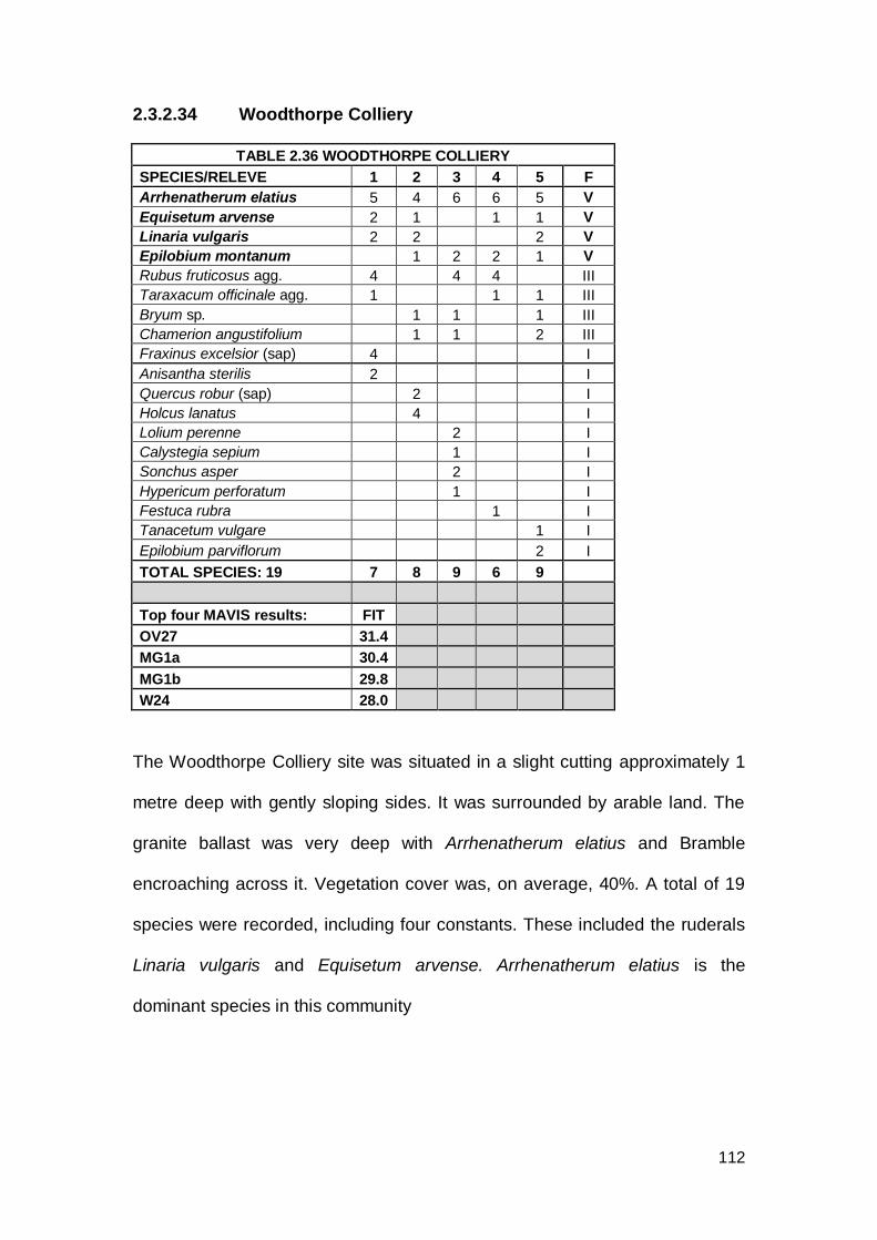
112
2.3.2.34 Woodthorpe Colliery
TABLE 2.36 WOODTHORPE COLLIERY
SPECIES/RELEVE 1 2 3 4 5 F
Arrhenatherum elatius 5 4 6 6 5 V
Equisetum arvense 2 1 1 1 V
Linaria vulgaris 2 2 2 V
Epilobium montanum 1 2 2 1 V
Rubus fruticosus agg. 4 4 4 III
Taraxacum officinale agg. 1 1 1 III
Bryum sp. 1 1 1 III
Chamerion angustifolium 1 1 2 III
Fraxinus excelsior (sap) 4 I
Anisantha sterilis 2 I
Quercus robur (sap) 2 I
Holcus lanatus 4 I
Lolium perenne 2 I
Calystegia sepium 1 I
Sonchus asper 2 I
Hypericum perforatum 1 I
Festuca rubra 1 I
Tanacetum vulgare 1 I
Epilobium parviflorum 2 I
TOTAL SPECIES: 19 7 8 9 6 9
Top four MAVIS results: FIT OV27 31.4 MG1a 30.4 MG1b 29.8 W24 28.0
The Woodthorpe Colliery site was situated in a slight cutting approximately 1
metre deep with gently sloping sides. It was surrounded by arable land. The
granite ballast was very deep with Arrhenatherum elatius and Bramble
encroaching across it. Vegetation cover was, on average, 40%. A total of 19
species were recorded, including four constants. These included the ruderals
Linaria vulgaris and Equisetum arvense. Arrhenatherum elatius is the
dominant species in this community
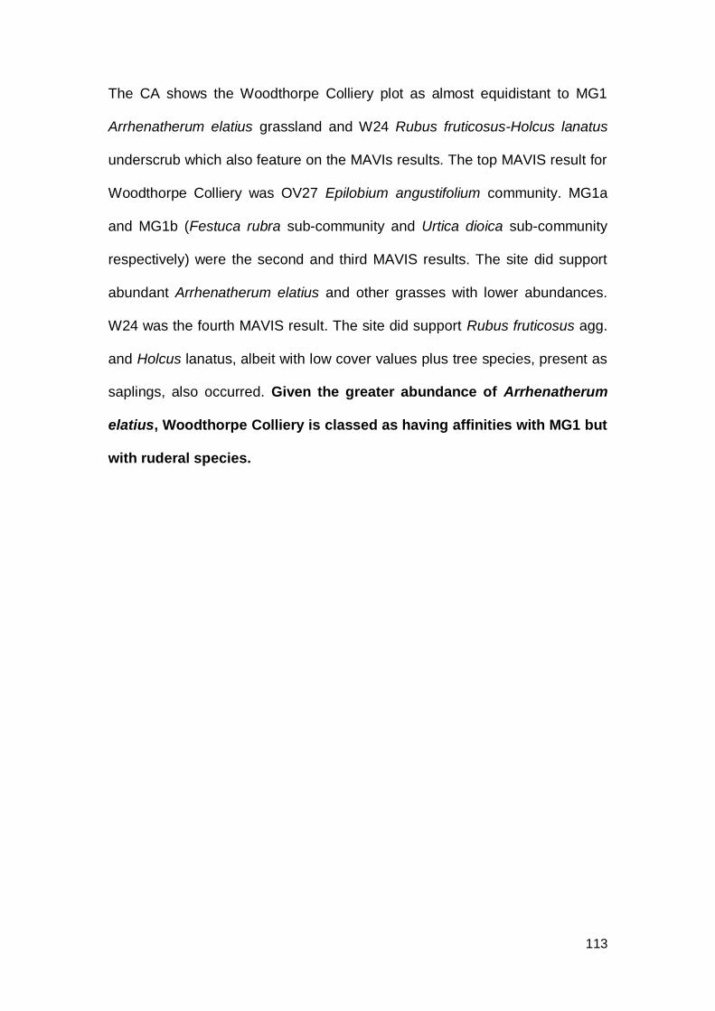
113
The CA shows the Woodthorpe Colliery plot as almost equidistant to MG1
Arrhenatherum elatius grassland and W24 Rubus fruticosus-Holcus lanatus
underscrub which also feature on the MAVIs results. The top MAVIS result for
Woodthorpe Colliery was OV27 Epilobium angustifolium community. MG1a
and MG1b (Festuca rubra sub-community and Urtica dioica sub-community
respectively) were the second and third MAVIS results. The site did support
abundant Arrhenatherum elatius and other grasses with lower abundances.
W24 was the fourth MAVIS result. The site did support Rubus fruticosus agg.
and Holcus lanatus, albeit with low cover values plus tree species, present as
saplings, also occurred. Given the greater abundance of Arrhenatherum
elatius, Woodthorpe Colliery is classed as having affinities with MG1 but
with ruderal species.
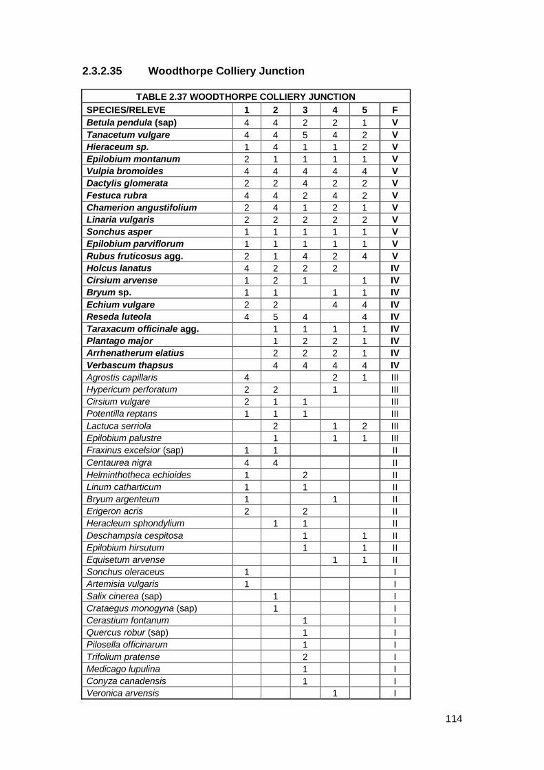
114
2.3.2.35 Woodthorpe Colliery Junction
TABLE 2.37 WOODTHORPE COLLIERY JUNCTION
SPECIES/RELEVE 1 2 3 4 5 F
Betula pendula (sap) 4 4 2 2 1 V
Tanacetum vulgare 4 4 5 4 2 V
Hieraceum sp. 1 4 1 1 2 V
Epilobium montanum 2 1 1 1 1 V
Vulpia bromoides 4 4 4 4 4 V
Dactylis glomerata 2 2 4 2 2 V
Festuca rubra 4 4 2 4 2 V
Chamerion angustifolium 2 4 1 2 1 V
Linaria vulgaris 2 2 2 2 2 V
Sonchus asper 1 1 1 1 1 V
Epilobium parviflorum 1 1 1 1 1 V
Rubus fruticosus agg. 2 1 4 2 4 V
Holcus lanatus 4 2 2 2 IV
Cirsium arvense 1 2 1 1 IV
Bryum sp. 1 1 1 1 IV
Echium vulgare 2 2 4 4 IV
Reseda luteola 4 5 4 4 IV
Taraxacum officinale agg. 1 1 1 1 IV
Plantago major 1 2 2 1 IV
Arrhenatherum elatius 2 2 2 1 IV
Verbascum thapsus 4 4 4 4 IV
Agrostis capillaris 4 2 1 III
Hypericum perforatum 2 2 1 III
Cirsium vulgare 2 1 1 III
Potentilla reptans 1 1 1 III
Lactuca serriola 2 1 2 III
Epilobium palustre 1 1 1 III
Fraxinus excelsior (sap) 1 1 II
Centaurea nigra 4 4 II
Helminthotheca echioides 1 2 II
Linum catharticum 1 1 II
Bryum argenteum 1 1 II
Erigeron acris 2 2 II
Heracleum sphondylium 1 1 II
Deschampsia cespitosa 1 1 II
Epilobium hirsutum 1 1 II
Equisetum arvense 1 1 II
Sonchus oleraceus 1 I
Artemisia vulgaris 1 I
Salix cinerea (sap) 1 I
Crataegus monogyna (sap) 1 I
Cerastium fontanum 1 I
Quercus robur (sap) 1 I
Pilosella officinarum 1 I
Trifolium pratense 2 I
Medicago lupulina 1 I
Conyza canadensis 1 I
Veronica arvensis 1 I

115
SPECIES/RELEVE 1 2 3 4 5 F
Urtica dioica 1 I
Hypericum humifusum 1 I
Leontodon hispidus 1 I
Betula pubescens (sap) 1 I
Geranium robertianum 1 I
TOTAL SPECIES: 53 29 31 33 26 31
Top four MAVIS results: FIT OV23d 33.6 W24 32.0 MG1a 31.8 MG1 31.5
The Woodthorpe Colliery Junction site was situated on a slight embankment,
surrounded by arable farmland. The granite ballast was deep and open, with
tufted vegetation and taller grasses growing closer to the rails. The average
vegetation cover was 50%. A total of 53 species were recorded, with many
species typical of ruderal habitats such as Erigeron acris and Conyza
canadensis. There were 21 constant species, including Tanacetum vulgare,
Echium vulgare, Linaria vulgaris and Reseda luteola.
The CA shows the Woodthorpe Colliery Junction plot as equidistant from
OV23 Lolium perenne–Dactylis glomerata community and MG1
Arrhenatherum elatius grassland but some distance from either. These
communities also feature in the MAVIS results. The top MAVIS result for
Woodthorpe Colliery Junction was OV23d (Arrhenatherum elatius–Medicago
lupulina sub-community). Dactylis glomerata is present as a constant with low
cover values but OV23 is typical of unmanaged but established grasslands
which is not similar to the community at Woodthorpe Colliery Junction. W24
Rubus fruticosus-Holcus lanatus underscrub was the second MAVIS result.
Both title species were present but with very low cover values. Tree species,

116
present as saplings, also occurred in low numbers across the ballast. The
number of grass species, however, and their combined abundance, identify
this community as closest to a grassland. MG1 is a better match than W24
due to the presence of seven species of grass and the tall Umbellifer
Heracleum sphondylium. However, this community has many ruderal
constants, which do not fit descriptions of MG1. The Woodthorpe Colliery
Junction site is classed as having affinities to MG1 but with many
ruderal species.
Table 2.37 below gives an overview of the results from each site.
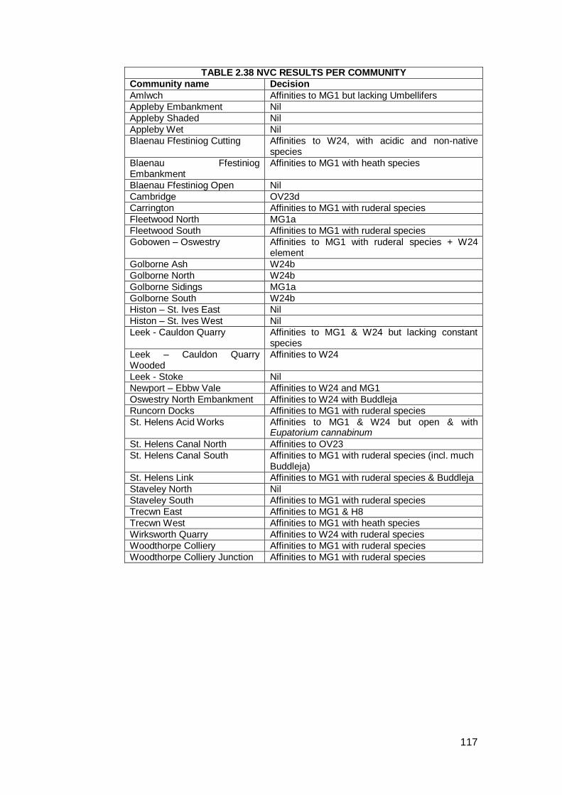
117
TABLE 2.38 NVC RESULTS PER COMMUNITY
Community name Decision
Amlwch Affinities to MG1 but lacking Umbellifers
Appleby Embankment Nil
Appleby Shaded Nil
Appleby Wet Nil
Blaenau Ffestiniog Cutting Affinities to W24, with acidic and non-native species
Blaenau Ffestiniog Embankment
Affinities to MG1 with heath species
Blaenau Ffestiniog Open Nil
Cambridge OV23d
Carrington Affinities to MG1 with ruderal species
Fleetwood North MG1a
Fleetwood South Affinities to MG1 with ruderal species
Gobowen – Oswestry Affinities to MG1 with ruderal species + W24 element
Golborne Ash W24b
Golborne North W24b
Golborne Sidings MG1a
Golborne South W24b
Histon – St. Ives East Nil
Histon – St. Ives West Nil
Leek - Cauldon Quarry Affinities to MG1 & W24 but lacking constant species
Leek – Cauldon Quarry Wooded
Affinities to W24
Leek - Stoke Nil
Newport – Ebbw Vale Affinities to W24 and MG1
Oswestry North Embankment Affinities to W24 with Buddleja
Runcorn Docks Affinities to MG1 with ruderal species
St. Helens Acid Works Affinities to MG1 & W24 but open & with Eupatorium cannabinum
St. Helens Canal North Affinities to OV23 St. Helens Canal South Affinities to MG1 with ruderal species (incl. much
Buddleja) St. Helens Link Affinities to MG1 with ruderal species & Buddleja
Staveley North Nil
Staveley South Affinities to MG1 with ruderal species
Trecwn East Affinities to MG1 & H8
Trecwn West Affinities to MG1 with heath species
Wirksworth Quarry Affinities to W24 with ruderal species
Woodthorpe Colliery Affinities to MG1 with ruderal species
Woodthorpe Colliery Junction Affinities to MG1 with ruderal species

118
2.4 DISCUSSION
Each railway community was unique in its species composition and relative
abundance. Most assemblages were difficult to assign to published NVC
communities.
Both the ‘objective’ approaches (MAVIS and CA) present problems. MAVIS
results are based on a Similarity Co-efficient which uses presence-absence
only. Hence the frequency of each species remains unutilised with this
method. CA does use species frequency but omits extent of coverage in each
relevé. Both frequency of occurrence and coverage per relevé are important
components of phytosociology. Consequently before allocating communities,
the phytosociological descriptions and floristic tables needed to be carefully
considered. This is borne out by the CA location of the Leek to Stoke plot
which, after analysing the NVC table and site description, appears to be
incorrectly placed.
Once this was done eight communities were identified that bear no
relationship to published NVC communities (Appleby Embankment, Appleby
Shaded, Appleby Wet, Blaenau Ffestiniog Open, Histon to St. Ives East,
Histon to St. Ives West, Leek to Stoke and Staveley North). Most of these
eight communities missed key components of an existing NVC community
(e.g. all of the Appleby communities did not support Rubus fruticosus agg. or
Arrhenatherum elatius). Many of them supported abundant bryophytes, which
are under-sampled in the NVC. All of the eight communities supported
combinations of ruderal species, including many as constants, which are

119
currently undescribed. Others, such as Blaenau Ffestiniog Open supported a
dominant species that does occur as a dominant in any similar NVC
community, in this case Molinia caerulea. Histon to St. Ives East and Histon to
St. Ives West are similar in that they support many ruderal species, some
non-natives and an element of calcareous species. Leek to Stoke is a unique
site in that it is very species-rich in comparison to the other sites and supports
many tall herbaceous species and ruderals. Rodwell et al (2000) attempted to
address the perceived gaps within the NVC. None of these eight sites match
the communities predicted within this work.
These apparently unique communities may have equivalents described on the
continent which will be the subject of the next chapter. Rodwell et al (2000)
recognised that some communities may fall under the continental Sisymbrion
officinalis type communities. It was suggested that a similar NVC community
would include Conyza canadensis, Sonchus oleraceus and Lactuca serriola.
No railway community had all of these species in combination but some of the
unattributable communities had them as constants (e.g. Cambridge - Conyza
canadensis, Appleby Embankment and Appleby Shaded - Sonchus
oleraceus; Histon to St. Ives West - Lactuca serriola).
By comparison six communities could be clearly ascribed to published NVC
descriptions. There are three sites which are ascribed to W24b Rubus
fruticosus–Holcus lanatus underscrub Arrhenatherum elatius–Heracleum
sphondylium sub-community (Golborne Ash, Golborne North and Golborne
South). There are two representatives of the MG1a Arrhenatherum elatius

120
grassland Festuca rubra sub-community (Fleetwood North and Golborne
Sidings) and one OV23d Lolium perenne–Dactylis glomerata community
Arrhenatherum elatius–Medicago lupulina sub-community (Cambridge).
Additionally there are twenty-one communities that contain key elements of
published NVC communities that also possess significant differences. Twelve
of these have an affinity to MG1 (see Table 2.38). These typically possess
Arrhenatherum elatius alongside other grassy components. They are distinct
from MG1 in that they contain ruderals as constants and lack forbs common
to MG1 (usually the large Umbellifers). Another group akin to MG1 possess a
heathy component usually alongside the grasses and some ruderals. A further
four sites have communities with key features of W24 with additional species
constant not previously described. These are typically ruderals although
Buddleja davidii is a significant component of some communities. Four
locations have assemblages with features of both MG1 and W24
communities. One location, St. Helens Canal North, has affinities to OV23 but
the typical OV23 habitat does not fit with the site.
Whether these twenty-one communities can be attributable to either MG1 or
W24 depends upon the breadth of circumscription of these two communities
and the means by which they are distinguished from each other given that
they form a successional sequence (Rodwell, 1992). Both MG1 and W24 are
extremely broad and rarely studied communities. MG1 is the sole lowland
ungrazed mesotrophic grassland described in the NVC and lacks a
comprehensive description although comparable communities have long been

121
recognised on the continent (e.g. Tuxen, 1955; Pfitzenmeyer, 1962). Although
Rodwell (1992) in his account of the MG1 community recognises its
occurrence on industrial habitats such as building sites, the physiognomic and
habitat descriptions are based upon typically closed communities on relatively
rich soil. Hence a common feature of the community as described are tall
Umbellifers with the closed sward severely limiting the occurrence of ruderals.
By comparison the communities surveyed in this study are open, allowing
abundant ruderals with the open, free-draining substrate limiting the
colonisation of more nutrient demanding species. This raises the question of
whether the communities described here akin to MG1 are part of a ruderal
sub-community of MG1, previously undescribed or represent a new
Arrhenatheretum. Where Arrhenatherum elatius is not dominant but a rank
sward supports abundant Holcus lanatus and Festuca rubra, Rodwell et al
(2000) recognised that this may also need a community description. In
addition, where dominant species were found which are not dominant in any
NVC community, such as Eupatorium cannabinum at the St. Helens Link site,
the question remains as to whether they represent a new community or again,
a new sub-community of the Arrhenatheretum.
Similar problems exist with the characterisation of W24. W24 is typically
described as a closed community and the question is whether the open
Rubus fruticosus agg. dominated communities recorded in this study fall
within the W24 community or represent a distinct phytosociological
association.

122
A further confusing factor is the floristic closeness of MG1 and W24. Both can
possess Arrhenatherum elatius and Rubus fruticosus agg. with abundances
overlapping. Rodwell (1992) describes a succession from an MG6 Lolium
perenne-Cynosurus cristatus grassland, a moderately species rich typically
grazed grassland, which then has grazing removed. This results in the
dominance of Arrhenatherum elatius with an MG1 the result. Further neglect
allows Bramble to become dominant producing the W24 community. A similar
successional sequence is also described starting from an OV23d Lolium
perenne–Dactylis glomerata community, a close sward community of resown
verges and fields which, if cutting ceases, may become MG1 with W24 to
follow. So an additional problem is where the MG1 (or MG1–like) community
ends and W24 (or W24-like) community begins.
The stand analysis has cut off a small eutrophic group (Group 1) and then
split the remainder between a more colonising Group 00 and a more
colonised Group 01. Group 00 splits into two distinct groups with 000
appearing transitional with 01 and 001 more extreme. Where Arrhenatherum
elatius is an indicator species it is found with a mix of species typical of either
scrub or open ruderal vegetation. Thus supporting the analysis elsewhere.
The Ellenberg and CSR analysis sheds little light on the community
differentiation. This is addressed by a more sophisticated analysis in Chapter
4.
If one examines the variation between other NVC communities where a single
species is dominant across a number of communities, for instance W10, W11,
123
W16 and W17 are all Quercus woodlands while MG5 and MG6 are both
Cynosurus grasslands, it is the associated vegetation and its physiognomy
that merit differentiation. Given the associated species with A. elatius are very
different from that described by Rodwell (1992) for MG1, with short lived
ruderal species rather than perennials, and that the physiognomy is also
markedly different, an open dynamic community rather than a closed one, I
consider that the community described here constitutes a new
Arrhenatheretum, previously undescribed from the UK.
124
CHAPTER 3 – A PHYTOSOCIOLOGICAL INVESTIGATION OF BRITISH DISUSED RAILWAY BALLAST VEGETATION USING THE BRAUN-BLANQUET SYSTEM 3.1 INTRODUCTION
Josias Braun-Blanquet started his phytosociological career studying alpine
vegetation and published this work in 1913. The Braun-Blanquet (hereafter
known as Br-Bl) methodology was developed by experienced plant ecologists,
including Br-Bl himself. They had vast knowledge of the communities present
in their region of study due to years spent surveying the land. From 1913
onwards, Br-Bl published prolifically in various Swiss publications (e.g. Br-Bl,
1915 and Br-Bl, 1931). Br-Bl’s seminal work Pflanzensoziologie in 1928
cemented the Zurich-Montpelier (Z-M) approach.
Br-Bl developed the idea of associations based purely on floristic composition.
He gave little weight to the dominance of each species and the physiognomy
of the community. Only after careful and thorough surveys of the same
community from a whole region, can the association be formed. The
association is a hierarchical system of alliance, order and class, each formed
from species found only within each community.
There are basically five steps to the original Br-Bl methodology:
1) Field description: determining a homogenous plant community in the
field and amassing the species lists from a minimum area relevé. Each
species is assigned an abundance score and a sociability score.
However, sociability (a measure of the extent of clustering) has more or
less been discarded by modern phytosociologists. This is due to three

125
key factors; the subjectivity of the score assigned to the species (which
depends largely on substrate), the lack of suitable statistical
determination of sociability and the fact that sociability represents the
growth form of the species, not its social physiognomy.
2) Aggregation of data into tables. The species lists would be copied by
hand and sorted by hand over many tables until patterns emerged of
groups of species always occurring together. Eventually an association
table was produced.
3) Using prior knowledge to check the species list against factors such
as environmental features (same soil type, aspect etc.).
4) Surveying for similar communities in the region.
5) Constructing an association table using all the available data from a
habitat.
A hierarchical system would emerge with the association with its faithful
species, followed by alliance, order and class. Despite the aggregation of data
into a table being relatively simple, the final analysis of the association table
required a level of knowledge of the plant community studied and the locality.
A criticism of the Br-Bl method was based upon the subjective nature of some
of this process (Shimwell, 1971).
One of the key features of the Br-Bl system is the concept of ‘faithful species’;
that is a species which occurs within one community and no other and often
referred to as fidelity. “Fidelity is the most fundamental notion of the Br-Bl
approach…it is also the concept through which (the Br-Bl school) differs from
126
all other schools of vegetation science” (Barkman, 1989). Poore (1955a,
1955b, 1955c & 1956) published a series of criticisms of the method, as he
attempted to apply it to British vegetation. Considering plant communities to
be fluid, he discarded the fidelity concept, explaining that a species could
occur within a continuum of communities. Similarly, continental ecologists
applying Br-Bl methods to their locality, without having the extensive plant
geographical knowledge of their region which the Br-Bl method requires,
found the same fidelity species in a number of plant communities (Shimwell,
1971).
However, fidelity continues to be a key component of phytosociological work
(e.g. Bruelheide, 2000). The modern approach is to address fidelity with
statistical analysis (e.g. Lososová et al, 2006 and Willner et al, 2009).
Following the International Botanical Congress in 1950, the Z-M system was
formally adopted as the recognised method for continental phytosociologists.
Consequently, most of Europe continued to, or started to, use Br-Bl’s method
for describing their vegetation e.g. Passarge (1957), Poore & McVean (1957),
Werger (1973) and Mirkin & Naumova (2009). Currently, the methodology is
used throughout continental Europe (Chytrý & Tichý, 2003, Favero-longo et
al, 2006 and Mirkin & Naumova, 2009). Further afield, Br-Bl is also chosen as
a method of vegetation classification with recent studies on Ethiopian riverine
habitats (Tikssa et al, 2009), Iranian woodlands (Hamzeh’ee et al, 2008) and
Californian sand dunes (Biondi & Cassavechia, 2001).
127
British ecologists have diverged from continental approaches, typically
following the views of Clements (1905) and others (Tansley, 1904 and Moss,
1910), who argued that the association, of ‘formation’ as they preferred to call
it, was not abstract but a successional entity. The plant community constantly
changed along seres before reaching a climax. Therefore, whilst the
continental ecologists were placing emphasis on a unit of pure vegetation,
British ecologists preferred geographical descriptions instead such as aspect,
slope etc.
In recent years, software has been developed to enable the relevés to be
entered, sorted and analysed. Turboveg (Hennekens & Schaminee, 2001)
was developed as a database to store multiple relevés. JUICE (Tichy, 2002)
was then created to work alongside Turboveg and analyse the data using a
variety of ordination packages such as COCKTAIL and TWINSPAN. Most
modern phytosociological work uses both Turboveg and JUICE e.g. Knollová
et al (2006), Šilc & Košir (2006), Cimalová & Lososová (2009) and Nowak et
al (2014a). However, Turboveg and JUICE are difficult to use in the UK. No
British ecologists appear to have used them and the inherent layout and
choices of nomenclature are aimed at continental relevés. Moreover, the
software packages cannot be used across countries, for example, to compare
datasets from different countries. The UK has never set up a database of
phytosociological relevés. Hence UK phytosociological studies use alternative
databases and methods of analysis (e.g. MAVIS).

128
Most of the early phytosociological work, both on the continent and in Britain,
took place in semi-stable habitats or semi-natural habitats, such as mountain
ranges, permanent grasslands or heathland (Shimwell, 1968). As the interest
in synanthropic vegetation developed, many were sceptical as to whether Br-
Bl could be used in disturbed habitats. For instance, Poore (1955) stated that
‘new’ habitats will not support faithful species and therefore they cannot be
formed into associations. Likewise, Pott (1992) considered that only well
developed communities could be classified into an association or sub-
association, ‘developing’ and ‘degenerated or regenerated’ communities were
impossible to classify.
By comparison, other authors believed that it was possible to classify
synanthropic vegetation. Becking (1957) considered that the advantage of the
Br-Bl methodology is that it could be used on ‘artificial, disturbed and
successional vegetation’, although requiring that the plant community must
have reached a ‘temporary equilibrium’. Communities such as the Sisymbrion
and Tanaceo-artemisietum were only ever described from urban
environments in Central Europe (Sukopp & Werner, 1983). Shimwell (in litt.
2006) always believed that Br-Bl would work on new vegetation.
Br-Bl has been frequently used on the continent to classify synanthropic
vegetation. For example, on weed and trampled vegetation the Czech
Republic (Lososová & Simonová, 2008 and Simonová, 2008), pioneer
vegetation on an asbestos mine in Italy (Favero-longo et al, 2006), vegetation
establishment on a marble quarry in Italy (Gentili et al, 2011) and city

129
vegetation in Slovenia (Šilc & Košir, 2006). Ecologists further afield have also
used the Br-Bl methodology in similar habitats e.g. Tikssa et al (2009) studied
plant communities of river corridors in Ethiopia and Nowak et al (2014b)
described weed associations from arable land in Krygyastan, Asia.
In contrast, few British ecologists have published work on urban or
synanthropic phytosociological communities. Hepburn (1942) described the
plant assemblages of the Barnack stone quarries. A study of the plant
colonisation of lime beds in Cheshire was undertaken by Lee & Greenwood
(1976). Silverside (1977) studied the phytosociology of British arable weeds.
Shaw (1992) described the plant colonisation and long-term plant
communities of pulverised fuel ash (PFA). Wright and Wheater (1993)
surveyed the vegetation on a disused railway line in Derbyshire. There have
been no recent peer-reviewed phytosociological studies of synanthropic
vegetation in the UK. This is reflected in the lack of publications in journal
databases (e.g. Web of Science). This study, therefore, is a unique
combination of a phytosociological approach to UK synanthropic vegetation
using the Br-Bl methodology.
The aim of this chapter is to identify disused railway ballast communities using
a modified Br-Bl approach. A comparison will be made to the National
Vegetation Classification (NVC) communities described in Chapter 2.

130
3.2 METHODS
3.2.1 Site selection
Sites were chosen for the presence of disused track with the rails in situ, and
therefore ballast also still intact. The railways also had to possess vegetation
so therefore had to have been abandoned for a minimum amount of time,
usually two years. The vegetation needed to support mainly ruderal plant
species and therefore, was generally in the early stages of succession;
disused lines which were heavily wooded or supported significant coverage of
scrub were not sampled (for example, sites dominated by Rubus fruticosus
agg. were often impenetrable so were not sampled). Moreover, heavily
wooded sites with rails in situ were rare. Sites were also chosen for
convenience of access, safety and initial broad geographic spread although
this was tempered by availability. Many of the disused lines were located in
ex-industrial areas with little pressure for development on the land. Others
were rural routes which served now defunct collieries or power stations. The
locations were selected by firstly finding disused railways (Baker 2004, 2010)
and OS paper maps. Aerial photography via Google earth and internet
searches were then used to determine whether track was still in situ. If a
disused track was very close to a live line it was not visited for health and
safety reasons. Details of sites surveyed are listed in table 1 below.

131
3.2.2 Sampling
At each site an approximately homogenous vegetation type was identified by
eye and surveyed using up to 10 relevés. The number of each relevé at each
site was restricted by the extent of the community present. Thus the survey
method is distinct from that in the previous chapter.
The maximum size of relevé needed to efficiently survey the vegetation was
found along the chosen homogenous stretch of railway line. The minimum
area calculation was used. In disused railway lines the vegetation typically
grows in the gaps between the sleepers so each relevé was approximately
1.4 metres wide and between 3 metres to 10 metres in length. This lends itself
well to the Br-Bl approach, which has no fixed relevé size, rather the relevé
size is incrementally increased until no new species are recorded. Vegetation
was recorded in two sleeper gaps initially with additional sleeper gaps being
added as long as any new plant species were found (i.e. increasing the size of
the relevé by one sleeper gap each time). Once no new plant species were
found then this was determined to be the maximum size of relevé needed.
The relevé size was determined afresh at each sample.
At each site all of the plants within the relevé were identified. A percentage
cover value of between 1%-100% was estimated for each species. The
traditional Br-Bl approach is to score each species along a six point
abundance score. However, percentage cover maintains detail and allows
potentially more discriminating computer analysis.

132
A field-recording sheet was created to input the raw data during the surveys.
An example is included in Chapter 2. The raw data for the Br-Bl analysis was
collected separately from the NVC data of Chapter 2. A sketch of the railway
line was added to the field sheet to aid visualising the railway during the write-
up.
In all cases, if plants, particularly lower plants, could not be identified in the
field then a sample of the plant was bagged and taken back to identify in more
detail (i.e. with a microscope and relevant keys). Vascular plants were named
following Stace (2010) and bryophytes using Smith (2004).
176 relevés were taken from a total of 35 sites from 22 different railway lines
(see Table 3.1).

133
TABLE 3.1 LIST OF RAILWAY LINE SITES SURVEYED
SITE CODE
SITE GRID REFERENCE
VICE-COUNTY
NO OF RELEVES
DATE SURVEYED
AM Amlwch SH 424913 52 5 16/07/2009
APC Appleby Cutting NY 694200 69 4 13/07/2009
APE Appleby Embankment NY 696195 69 4 13/07/2009
APW Appleby Wet NY 694199 69 3 13/07/2009
BFC Blaenau Ffestiniog Cutting SH 705441 48 6 16/09/2009
BFE Blaenau Ffestiniog Embankment SH 707439 48 5 16/09/2009
BFO Blaenau Ffestiniog Open SH 704443 48 3 16/09/2009
CA Cambridge TL 428639 29 5 23/08/2004
CN Carrington SJ 753903 58 10 04/05/2007
FN Fleetwood North SD 328457 60 5 07/07/2009
FS Fleetwood South SD 342428 60 5 07/07/2009
G-O Gobowen – Oswestry SJ300313 40 5 17/07/2009
GA Golborne Ash SJ 603993 59 3 03/08/2009
GN Golborne North SJ 602991 59 5 03/08/2009
GSI Golborne Sidings SJ 603989 59 6 04/08/2004
GS Golborne South SJ 601988 59 5 03/08/2009
H-ST.IE
Histon – St. Ives East TL 397681 29 3 21/07/2007
H-ST.IW
Histon – St. Ives West TL 363694 29 5 21/07/2007
L-C Leek – Cauldon Quarry SK 022538 39 10 12/05/2005
L-CW Leek – Cauldon Quarry Wooded SJ 996545 39 3 12/05/2005
L-S Leek – Stoke SJ 939538 39 6 04/05/2005
N-EB Newport – Ebbw Vale ST 210965 41 3 22/06/2007
ONE Oswestry North Embankment SJ 297302 40 5 17/07/2009
RD Runcorn Docks SJ 499823 58 10 23/07/2009
ST.HA St. Helens Acid Works SJ 527938 58 5 29/07/2004
ST.CANN
St. Helens Canal North SJ 515950 59 5 06/07/2009
ST.CANS
St. Helens Canal South SJ 517949 59 5 06/07/2009
ST.HL St. Helens Link SJ 527939 58 4 21/06/2004
SN Staveley North SK 440741 57 5 22/08/2009
SS Staveley South SK 442739 57 5 22/08/2009
TE Trecwn East SM 963324 45 3 10/09/2010
TW Trecwn West SM 956320 45 5 10/09/2010
WQ Wirksworth Quarry SK 288545 57 4 18/07/2004
WC Woodthorpe Colliery SK 459744 57 5 13/08/2009 WCJ Woodthorpe Colliery Junction SK 456742 57 5 13/08/2009
3.2.3 Statistical Analysis
The survey results were entered into Excel. The software program R was
used to undertake multivariate analysis of all 176 relevés. This incorporated
both PCA analysis and NMDS. In addition, Ward's hierarchical cluster
analysis was carried out (Ward, 1963), which is widely used for this type of
data (e.g. Lososová et al, 2006).

134
For PCA and NMDS, all of the data was included. In addition, the data was
run with the exclusion of species found in both less than 10% of the relevés
and less than 20% of the relevés. PCA was also undertaken with and without
the Hellinger transformation.
Following cluster analysis, species characteristic of each cluster were
identified using Indicator Values (IndVal, Dufrene and Legendre, 1987). This
assigns a value (max of 1.00) for each species, taking into account its
exclusivity (its faithfulness to a cluster) and its fidelity (the extent to which it is
found within a cluster). A value of 1 shows that a species is only found in a
single cluster and is found in all the relevés within that cluster. The statistical
significance of each IndVal is calculated based upon a randomization
approach. A significant IndVal greater than or equal to 0.400 was taken as a
species that can be used to characterize that cluster.

135
3.3 RESULTS
3.3.1 General
A total of 246 species were recorded across all of the sites using the Br-Bl
method. Relevé size varied between 3 and 13 sleeper gaps. The mean relevé
size was 10 sleeper gaps. The minimum number of relevés on any site was 3.
64 species are restricted to just one site. Table 3.2 shows the data for the
species present in twenty or more relevés. Arrhenatherum elatius, Rubus
fruticosus agg., Holcus lanatus and Festuca rubra were the most abundant
species, each occurring in at least 50% of relevés. The mean coverage per
relevé in which a species is present is typically low with the most widespread
species (Arrhenatherum elatius) showing the highest value (15%). All other
species have a mean % cover of 11% or less.

136
Table 3.2 Species present in 20 or more relevés, proportion of relevés present and mean and standard deviation of % cover in relevés present
Species
Number relevés present
% Relevés present
Mean % coverage
St.dev % coverage
Arrhenatherum elatius 134 76 15 14
Rubus fruticosus agg. 102 58 9 8
Holcus lanatus 88 50 5 6
Festuca rubra 81 45 9 13
Taraxacum officinale agg. 80 45 2 1
Senecio jacobaea 72 41 2 2
Chamerion angustifolium 63 36 2 2
Dactylis glomerata 60 34 4 6
Epilobium montanum 57 32 1 1
Agrostis capillaris 52 30 2 2
Brachythecium rutabulum 48 27 5 6
Epilobium parviflorum 48 27 1 1
Lolium perenne 41 23 6 9
Sonchus asper 36 20 2 1
Geranium robertianum 35 20 9 18
Plantago lanceolata 35 20 2 3
Vulpia bromoides 31 18 11 12
Linaria vulgaris 29 16 2 2
Agrostis stolonifera 26 15 6 11
Fraxinus excelsior 26 15 9 13
Heracleum sphondylium 26 15 2 2
Betula pendula 23 13 6 7
Urtica dioica 22 12.5 1 0
Plantago major 22 12.5 1 1
Crataegus monogyna 22 12.5 1 1
Leontodon hispidus 21 12 2 2
Geum urbanum 21 12 3 3
Galium aparine 21 12 1 0
Poa annua 21 12 2 2
Deschampsia cespitosa 20 11 5 5
Equisetum arvense 20 11 4 5
Hypochaeris radicata 20 11 2 1
3.3.2 PCA Analysis
The PCA analysis proved to be problematic. PCA treats zeroes as similarities
between relevés. The classic 'horseshoe' pattern emerged from using PCA on
all of the relevés (see Figure 3.1). Removing the species that occurred in less
than 10% of the relevés and then removing the species that occurred in less

137
than 20% of the relevés made no difference (figure not shown). This
continued to give the horseshoe shape. Removing species also potentially
reduced the effectiveness of the Br-Bl approach as the species which were
removed may be fidelity species. Thus PCA was dismissed as a method of
analysis.
Figure 3.1 - PCA graph showing the 'horseshoe' pattern which emerged due to PCA treating zeroes as similarities between relevés and therefore PCA was dismissed as a method of analysis.

138
3.3.3 NMDS
NMDS is a multivariate approach that does not treat shared zeroes as
evidence of similarity.
Figure 3.2 - NMDS graph results - the dots show the position of individual relevés, colour denotes relevé locations (see Table 3.1 for key to site codes). The graph shows no clear clustering pattern.
Figure 3.2 shows there to be no clear clustering of the relevés. Loose
clustering occurs, particularly of relevés from the same site such as Runcorn
Docks (RD - fuchsia) and Amlwch (AM - black). The graph also shows
clustering of relevés that are not from the same site such as Blaenau
Ffestiniog Embankment (BFE - dark green) and Gobowen – Oswestry (G-O -
mint green).
139
3.3.4 Hierarchical Cluster Analysis
The results from the hierarchical cluster analysis show clear splits in the data
(see Figure 3.3). At the highest level, there is a clear two-way split which is
not equal in size.
Several species with an IndVal greater than or equal to 0.400 were found in
each level of clustering. These species are presented with the main clusters in
Figure 3.3. Figure 3.4 shows the entire hierarchical clustering of all relevés.
Significant IndVals <0.400 do exist, see Table 3.3. However these were not
used to characterise a cluster.

140
Table 3.3 IndVal data
IndVal Fidelity Exclusivity Mean % cover Mean % cover
in cluster elsewhere
CLUSTER A
Epilobium ciliatum 0.9110 95% 95% 2 1
Geranium robertianum 0.7633 84% 46% 18 2
Fraxinus excelsior 0.4305 53% 38% 15 5
Holcus lanatus 0.3807 79% 19% 12 4
Lotus corniculatus 0.2865 32% 86% 18 5
Rhododendron ponticum 0.2632 26% 100% 1 NA
Calluna vulgaris 0.2632 26% 100% 1 NA
Polytrichum commune 0.2105 21% 57% 15 NA
0.2105 21% 100% 7 NA
Rhytidiadelphus squarrosus 0.1705 32% 38% 3 4
Viola riviniana 0.1701 21% 67% 1 1
Molinia caerulea 0.1579 16% 100% 37 NA
Hypericum tetrapterum 0.1579 16% 100% 1 NA
Geum rivale 0.1579 16% 100% 1 NA
Teucrium scorodonia 0.1427 21% 67% 2 4
Ulex gallii 0.1053 11% 100% 1 NA
Dicranum scoparium 0.1053 11% 100% 16 NA
CLUSTER B
Eupatorium cannabinum 0.8038 93% 72% 8 16
Agrostis stolonifera 0.6478 71% 40% 11 2
Epilobium hirsutum 0.2986 36% 38% 5 2
Festuca ovina 0.2587 57% 50% 2 3
Buddleja davidii 0.1862 29% 27% 21 13
Salix cinerea 0.1786 21% 60% 2 3
Senecio squalidus 0.1429 14% 100% 1 NA
Euphrasia officinalis agg 0.1334 14% 67% 3 2
CLUSTER C
Arrhenatherum elatius 0.3589 100% 44% 25 10
Rubus fruticosus agg 0.2884 83% 32% 10 8
Hypnum cupressiforme 0.2455 28% 65% 14 2
Bryoerythrophyllum recurvirostrum 0.1581 18% 70% 2 1
CLUSTER D
Vulpia bromoides 0.8461 100% 74% 23 4
Galium aparine 0.7873 100% 50% 1 1
Anthriscus sylvestris 0.6928 80% 50% 2 2
Pimpinella saxifraga 0.6000 60% 100% 2 NA
Veronica arvensis 0.5930 80% 67% 1 2
Picris echioides 0.5365 70% 59% 2 1
Sonchus asper 0.4344 80% 42% 2 2
Linum catharticum 0.3750 50% 42% 1 2
Crepis vesicaria 0.3474 40% 80% 1 4
Hypochaeris radicata 0.2752 50% 35% 2 2
Centaurium erythraea 0.2496 30% 36% 1 1
Rumex crispus 0.2236 30% 43% 2 1
Cerastium fontanum 0.2131 40% 43% 1 1
Senecio jacobaea 0.2100 90% 22% 1 2
Conyza canadensis 0.1974 30% 33% 2 4
Senecio viscosus 0.1943 40% 33% 1 3
Blackstonia perfoliata 0.1000 10% 100% 1 NA
Table 3.3 Species significantly determined with each cluster determined by indicator value (IndVal, Dufrene & Legendre, 1987). IndVal is a product of exclusivity, the faithfulness to a cluster, and its fidelity, the extent to which it is found in that cluster. Also listed is the mean % cover both within the cluster with which it is significantly associated and the remaining relevés. Species used to characterise a cluster are shown in bold.
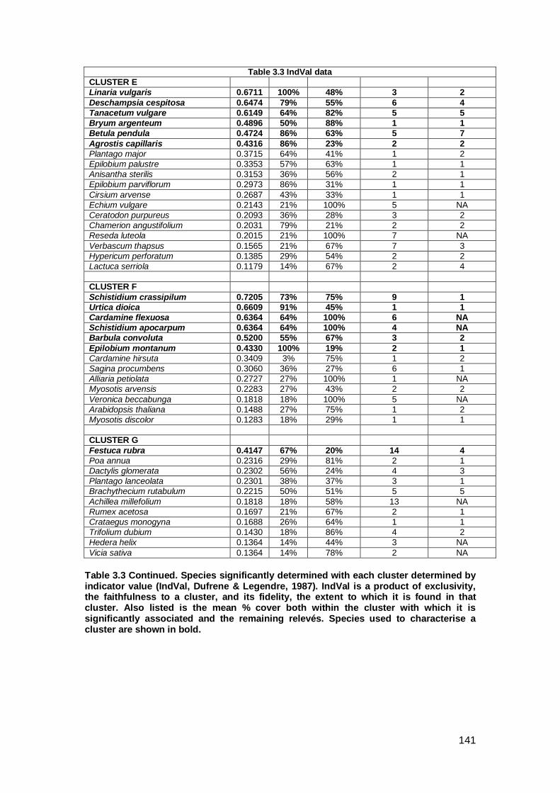
141
Table 3.3 IndVal data
CLUSTER E
Linaria vulgaris 0.6711 100% 48% 3 2
Deschampsia cespitosa 0.6474 79% 55% 6 4
Tanacetum vulgare 0.6149 64% 82% 5 5
Bryum argenteum 0.4896 50% 88% 1 1
Betula pendula 0.4724 86% 63% 5 7
Agrostis capillaris 0.4316 86% 23% 2 2
Plantago major 0.3715 64% 41% 1 2
Epilobium palustre 0.3353 57% 63% 1 1
Anisantha sterilis 0.3153 36% 56% 2 1
Epilobium parviflorum 0.2973 86% 31% 1 1
Cirsium arvense 0.2687 43% 33% 1 1
Echium vulgare 0.2143 21% 100% 5 NA
Ceratodon purpureus 0.2093 36% 28% 3 2
Chamerion angustifolium 0.2031 79% 21% 2 2
Reseda luteola 0.2015 21% 100% 7 NA
Verbascum thapsus 0.1565 21% 67% 7 3
Hypericum perforatum 0.1385 29% 54% 2 2
Lactuca serriola 0.1179 14% 67% 2 4
CLUSTER F
Schistidium crassipilum 0.7205 73% 75% 9 1
Urtica dioica 0.6609 91% 45% 1 1
Cardamine flexuosa 0.6364 64% 100% 6 NA
Schistidium apocarpum 0.6364 64% 100% 4 NA
Barbula convoluta 0.5200 55% 67% 3 2
Epilobium montanum 0.4330 100% 19% 2 1
Cardamine hirsuta 0.3409 3% 75% 1 2
Sagina procumbens 0.3060 36% 27% 6 1
Alliaria petiolata 0.2727 27% 100% 1 NA
Myosotis arvensis 0.2283 27% 43% 2 2
Veronica beccabunga 0.1818 18% 100% 5 NA
Arabidopsis thaliana 0.1488 27% 75% 1 2
Myosotis discolor 0.1283 18% 29% 1 1
CLUSTER G
Festuca rubra 0.4147 67% 20% 14 4
Poa annua 0.2316 29% 81% 2 1
Dactylis glomerata 0.2302 56% 24% 4 3
Plantago lanceolata 0.2301 38% 37% 3 1
Brachythecium rutabulum 0.2215 50% 51% 5 5
Achillea millefolium 0.1818 18% 58% 13 NA
Rumex acetosa 0.1697 21% 67% 2 1
Crataegus monogyna 0.1688 26% 64% 1 1
Trifolium dubium 0.1430 18% 86% 4 2
Hedera helix 0.1364 14% 44% 3 NA
Vicia sativa 0.1364 14% 78% 2 NA
Table 3.3 Continued. Species significantly determined with each cluster determined by indicator value (IndVal, Dufrene & Legendre, 1987). IndVal is a product of exclusivity, the faithfulness to a cluster, and its fidelity, the extent to which it is found in that cluster. Also listed is the mean % cover both within the cluster with which it is significantly associated and the remaining relevés. Species used to characterise a cluster are shown in bold.

142
The cluster analysis identified seven major clusters (A-G; Fig 3.3). Clusters A,
B and C are in major cluster 1, characterised by Arrhenatherum elatius
(IndVal = 0.75) and Rubus fruticosus agg. (0.45). Cluster B and C are in major
sub-cluster 4, characterised by Arrhenatherum elatius (0.47). Arrhenatherum
elatius (0.35) characterises cluster C with Rubus fruticosus agg. and two
moss species. Epilobium ciliatum (0.91), Geranium robertianum (0.76) and
Fraxinus excelsior (saplings) (0.43) characterise cluster A while Eupatorium
cannabinum (0.80) and Agrostis stolonifera (0.65) characterise Cluster B.
There are 19 relevés in Cluster A, from the following railway sites: Blaenau
Ffestiniog Open, Blaenau Ffestiniog Embankment, Blaenau Ffestiniog
Cutting, Trecwn East and Trecwn West. Cluster B is comprised of 14 relevés
from the following railway sites: St. Helens Link, St. Helens Acid Works, St.
Helens Canal South and Fleetwood South. Cluster C is comprised of 40
relevés from the following railway sites: Blaenau Ffestiniog Embankment,
Cambridge, Golborne South, Oswestry North Embankment, Woodthorpe
Colliery, Staveley North, Fleetwood South, Golborne South, Newport - Ebbw
Vale, St. Helens Acid Works, Golborne Ash, Leek - Cauldon Quarry Wooded
and Leek - Cauldon Quarry.
Major cluster 2 is characterised by the three species (Senecio jacobaea, 0.47;
Festuca rubra, 0.44 and Taraxacum officinale agg. 0.40). Major cluster 2 in
turn is split into two major sub-clusters (5 and 6). Major Sub-cluster 5 is
characterised by Vulpia bromoides (0.91) and Linaria vulgaris (0.44). It
incorporates cluster D with seven indicator species (V. bromoides, 0.84;

143
Galium aparine, 0.79; Anthriscus sylvestris, 0.69; Pimpinella saxifraga, 0.60;
Veronica arvensis; 0.59, Picris echinoides, 0.54 and Sonchus asper, 0.43),
while cluster E is also typified by a large suite of species (L. vulgaris, 0.67;
Deschampsia cespitosa, 0.64; Tanacetum vulgare, 0.61; Bryum argenteum,
0.49; Betula pendula, 0.47 and Agrostis capillaris, 0.43). Major sub-cluster 6 is
characterised by F. rubra (0.4) and this is split into cluster F characterised by
six species (Schistidium crassipilum, 0.72; Urtica dioica, 0.66; Cardamine
flexuosa, 0.63; Schistidium apocarpum, 0.64; Barbula convoluta, 0.52 and
Epilobium montanum, 0.433) while Cluster G is characterised by F. rubra only
(0.4).
There are 10 relevés in Cluster D from Runcorn Docks only. 14 relevés form
Cluster E from the following railway sites: Woodthorpe Colliery Junction,
Staveley South and Staveley North. Cluster F is comprised of 11 relevés from
the following railway sites: Appleby Embankment, Appleby Wet and Appleby
Cutting. Cluster G is the largest cluster, comprised of 66 relevés. These are
from the following railway lines: Golborne North, St. Helens Canal North,
Fleetwood North, Leek - Cauldon Quarry Wooded, Blaenau Ffestiniog Cutting,
Wirksworth Quarry, Oswestry North Embankment, Newport - Ebbw Vale,
Gobowen - Oswestry, Histon - St. Ives West, Histon - St. Ives East, Leek -
Stoke, Leek - Cauldon Quarry, Golborne South, Amlwch and Carrington.
Cluster G is the largest with 66 samples. Most clusters contain relevés from
more than one location, the exception being Cluster D, in which all of the

144
relevés are from Runcorn Docks. There is no relationship between number of
relevés in a cluster and the number of significant indicator species.
The block diagram in Figure 3.5 gives a view of the indicator species
distribution per cluster. This is a visualisation of the data used to generate the
indicator values. While species are found in blocks which typify the cluster, if
found in the majority of relevés of that cluster they are also likely to occur
sporadically in other clusters.

145
Figure 3.3 - Hierarchical Cluster Analysis of disused railway lines, showing six major splits. The numbers in circles denote major splits and the letters denote final clusters. The numbers denote the number of relevés within that cluster.

146
Figure 3.4 - Hierarchical Cluster Analysis of all relevés. Differently coloured symbols identify the different sites, as presented in the key below.

147

148
Table 3.4. Block diagram showing distribution of species across clusters. Species with significant Indicator Values are in the left hand column. Relevés are sorted by clusters which are delineated by the thick vertical lines. Blue colouring indicates presence of the species in that relevé, the darker the blue colour the higher the percentage cover.

149
3.4 DISCUSSION
A total of 246 species were recorded across all of the sites using the Br-Bl
method. This is a slight decrease in the number recorded using the NVC
method, described in Chapter 2, where 268 species were recorded in total
across all of the sites. This difference is due to the slightly smaller area
surveyed with some Br-Bl relevés. Different Br-Bl relevé sizes sometimes
demand statistical treatment to make relevés comparable (e.g. Chytrý &
Otýpková, 2003). However, the close similarity of relevé sizes across the
survey render such processes unnecessary.
32 species are found in at least 20 relevés, although only three species are
found in over 50% of relevés. Hence the vast majority of species (214) are
found in only a few relevés. All species are found at very low coverage
reflecting the open vegetation characteristic of early successional vegetation.
Multivariate analysis, although frequently used in vegetation studies, proved
of little value in this study. Cluster analysis proved more useful, an approach
some authors use exclusively (e.g. Angiolini et al, 2006), although some
authors have found both multivariate analysis and hierarchical cluster analysis
to be useful e.g. Greller et al (2000). PCA analysis resulted in the horseshoe
shape and was subsequently dismissed. NMDS showed no clear clustering of
the relevés. No pattern emerged from the data using NMDS whereas cluster
analysis proved to be more revealing with clear splits in the composition of the
relevés.

150
Seven communities are apparent from the hierarchical clustering. Clusters A,
B and C are split from Clusters D, E, F and G by the presence of
Arrhenatherum elatius in the former clusters. Within this split, lie further splits
based on the presence of either Fraxinus excelsior or Geranium robertianum,
i.e. a move ultimately towards scrub and shaded communities and the split
towards damper communities with Eupatorium cannabinum and Agrostis
stolonifera.
The community identified by Cluster A is dominated by Epilobium ciliatum and
Geranium robertianum with abundant Fraxinus excelsior seedlings. This is
then a mixture of grass species (Holcus lanatus, Molinia caerulea), which may
be present with woody species (Rhododendron ponticum, Calluna vulgaris
and Ulex gallii) and various forbs of low frequency (see Table 3.3).
The Cluster B community is distinct, featuring abundant Eupatorium
cannabinum and Agrostis stolonifera with occasional woody components such
as Buddleja davidii and Salix cinerea, along with a mixture of forbs (Table
3.3).
Arrhenatherum elatius is a feature of both communities described above,
however, it is most strongly linked to Cluster C, which is a loose assemblage
of mosses (Hypnum cupressiforme and Bryoerythrophyllum.recurvirostrum)
and Rubus fruticosus agg.

151
Of the four communities in the other major cluster, Cluster D is by
characterised by Vulpia bromoides occurring with Galium aparine, Anthriscus
sylvestris and Picris echioides.
The fifth community features a combination of forbs (Linaria vulgaris,
Tanacetum vulgaris) with grass species (Deschampsia cespitosa, Agrostis
capillaris). Woody species are represented by Betula pendula. Other species
typifying this community are medium-sized forbs (e.g. Epilobium parviflorum,
Cirsium arvense and Chamerion angustifolium).
The sixth cluster is dominated by Urtica dioica with many moss species (e.g.
Schistidium crassipilum and Schistidium apocarpum) and small forbs (e.g.
Cardamine hirsuta, Sagina procumbens and Myosotis arvensis).
The final community is another loose aggregation of species characterised by
Festuca rubra with a mixture of grass species (Dactylis glomerata and Poa
annua) and medium-sized forbs (e.g. Achillea millefolium and Plantago
lanceolata).
There are no absolute fidelity species (Figure 3.4, Table 3.3, Table 3.4).
However this pattern is typical in ruderal communities, therefore separation is
determined by a stronger association of species than elsewhere in the sites
surveyed. No comparative studies have been found of ruderal communities,
which use Indicator Values to determine community composition.

152
Plant communities with similar constant species to the NVC communities
(described in Chapter 2) emerged from the Br-Bl data. Major cluster 1, which
is dominated by Arrhenatherum elatius, is commensurate with the findings of
the NVC results, which shows a cluster of sites which support the basics of an
MG1 grassland but with a ruderal component and a lack of umbellifers.
Cluster A includes a strong ruderal component (e.g. Epilobium ciliatum) with
heathland species, another affinity with the NVC results. Another set of sites
within the NVC support MG1 grassland with woody elements. This can be
aligned to Cluster B, featuring Buddleja davidii and Salix cinerea as
components. The four communities in the other major cluster are dominated
by ruderal species. Few affinities were found within the NVC data to Open
Vegetation (OV) communities. The grass-dominated OV23 was loosely
aligned to a few sites. Cluster G has Festuca rubra as an indicator species.
Hierarchical clustering may be more sensitive to the differences in the
community composition as a result of the finer scale of analysis, 1-100 per
species per relevé, compared to NVC analysis which uses a five point Domin
score per species per site. In addition, differences between the results of the
Br-Bl approach and the results of the NVC approach may be due to
differences in the approach to analysis.
It is difficult to compare the results of the Br-Bl hierarchical clustering in this
study with continental studies. Although authors on the continent have used
hierarchical clustering to describe and name plant communities from ruderal
sites (e.g. Lososová et al, 2006; Simonová, 2008 and Lasić et al, 2014), none

153
of the species or plant assemblages published resemble those found during
this study. Moreover, previously described continental ruderal plant
associations do not resemble those found here. This raises the possibility that
these communities are unique to the UK, a product of the habitat combined
with the oceanic climate.
The lack of published work in this field and hence the lack of knowledge of the
potential architects of community composition means that there is a need to
investigate the factors. Chapter 4 will investigate the environmental variables
on each of the sites and explore possible environmental reasons for the
community composition.

154
CHAPTER 4 – FACTORS INFLUENCING COMMUNITY COMPOSITION
4.1 INTRODUCTION
The successional process and the drivers behind it have long been debated.
Many early ecologists believed in the climax community, i.e. that there were
distinct stages from pioneer colonisation to a stable community, determined
by the ability of the initial successful colonists to tolerate extreme conditions
through to the competitive abilities of the species present within the climax
community (Clements, 1936). This approach is described in the classic sand
dune succession studies (Ranwell, 1960 and Pye, Saye & Blott, 2007). Other
ecologists have argued that succession was a random and unpredictable
event, with individual species exhibiting variation in their response to
environmental factors such as disturbance and stress (e.g. Gleason, 1917).
Studies have been carried out on the factors influencing community
composition at various successional stages. While the view of a deterministic
view of succession based on intrinsic plant characteristics, primarily life
strategies (e.g. competitiveness) is still widely held (Grime, 2001), this is far
from a universal viewpoint. Individual adaptations to disturbance and stress
are considered more important by some authors (e.g. Caccianiga et al, 2006)
while the role of stochastic processes is borne out in large scale succession
studies such as tree species distribution in Europe since the Ice Age
(Svenning & Skov, 2007). This debate is still current, leading to early
successional processes being the subject of much research, although the
155
recognised contribution of stochastic factors has led it more recently to
frequently be termed vegetation dynamics (Pickett et al, 2008).
More recently, a 'reductionist' approach has been developed, to try and
predict the successional process. This has meant ecologists studying
vegetation processes at a local scale, rather than a global or regional scale.
The view is that ecosystems are in a constant state of change and the various
components respond individualistically. Therefore, succession is not
recognised as a procession of competitive species but as a random
assemblage of species being constantly replaced in a mosaic of patch
communities (Walker & del Moral, 2003). Therefore, predicting succession is
difficult and that in any given locality, there can be multiple pathways that the
successional stages can take. This was the conclusion on the dune systems
in the Netherlands (van der Maarel et al, 1985) and on deglaciated land in
Alaska (Chapin et al, 1994). Hence phytosociologists currently struggle with
predicting succession because of the ecological complexities at the
community level and the individual plant species level (Walker, 2012).
Nevertheless, modern ecologists have also sought to identify successional
processes based upon abiotic and biotic variables. For instance climate has
long been known as a factor influencing community composition (e.g. Peinado
et al, 2005a & 2005b, & Lososová et al, 2006). Climate change has refocused
studies into climate affecting plant communities, especially those close to
human settlements (e.g. Turner et al, 2004). Hence environmental factors
such as rainfall, aspect, altitude, mean temperatures are typically incorporated
156
into vegetation dynamic studies. For instance Hodge & Harmer (1996) studied
rainfall, the soil characteristics and the depth of vegetation penetration when
investigating woody colonisation, while local moisture levels have been shown
to vegetation establishment (Prach et al, 2013). Seed rain has been
demonstrated to be a major influence in the direction of succession (Evans &
Dahl, 1955; Lanta & Leps, 2009).
Time is also an important factor in succession (e.g. Chapin et al, 1994). Rates
of species turnover are known to decline with time since abandonment or
disturbance (Walker & del Moral, 2003). This is due to a number of factors
including increase in shading from long-term plant species, lack of open
ground making establishment difficult for pioneer species and increase in
nutrients within the humic layer allowing for a healthier plant growth and
longer term survival.
In synanthropic habitats the nature of the substrate is an important limiting
factor, given that ex-industrial sites tend to have soils of poor structure and
which are often heavily contaminated. This includes poor water retention and
poor nutrient levels (Hiller, 2000) and heavy metal content (Malawska &
Wilkomirski, 2000). For example, lead was found to be the most limiting factor
for plant diversity during a study of old lead mines in the Pennines (Clark &
Clark, 1981). The pH of the substrate can also be an important variable (e.g.
Hall, 1959). McLaughlin & Crowder (1988) studied the environmental factors
affecting the distribution of two grass species; Agrostis gigantea and Poa
pratensis, on copper-nickel mine tailings in Ontario, Canada. Despite the

157
substrate being contaminated with iron, nickel and copper, pH and moisture
significantly affected distribution of grass species.
Nearly all studies of plant establishment on ex-industrial land have
investigated the nutrient load in the substrate. Nitrogen, Potassium, Calcium,
Magnesium and Phosphorus are commonly measured. The nutrient load
helps to understand the ability for plants to not only colonise but to persist
within the site. For example, a study of china clay waste in Cornwall (Roberts
et al, 1981), found that the Potassium, Calcium and Magnesium content of the
waste was lower than the control site but that the Phosphorus levels were
relatively high, a product of the ease with which these elements are leached
out of the china clay waste whereas Phosphorus is more immobile in soil,
therefore resistant to leaching.
In previous chapters, the suitability of disused railway lines as study sites for
phytosociological work has been discussed. They are a finite habitat, built to a
similar specification throughout the UK with a well-drained granite ballast.
Thus the starting point of all disused sites is very similar. Railway ballast is
typically composed of hard, angular granite chippings, the main purposes of
which are to distribute stress and allow drainage. Historically (pre-1970’s) a
variety of mediums have been used, mainly ash, until steam locomotives
ceased to be used, but also broken bricks and clay (Claisse & Calla, 2006).
Since the nationalisation of the railways, the British standard has been granite
of 50-32mm in size (Granite R/Track Spec EN13450) (NR/L2/TRK/1800)
(National Rail). Therefore the substrate is fixed and not a variable influence on

158
plant succession. Moreover, plant establishment is prevented while the ballast
is in use due to annual herbicide treatment. Hence the development of
vegetation following closure presents a natural experiment where the effects
of time and environment and then soil development can be studied
(Suominen, 1979).
This chapter investigates the potential role of environmental, edaphic and
temporal factors on community development and thus to ascertain the
predictability of ruderal community composition. These factors are considered
across all the relevés and at the level of the seven communities identified in
the previous chapter.
The following factors were utilised to investigate whether there is a pattern to
ruderal plant community composition: time since abandonment, aspect, slope,
altitude, mean rainfall, mean temperature, pH, soil moisture content, soil
organic content, and the following metals: Magnesium, Lead, Cadmium,
Potassium, Calcium, Copper and Nickel. The role of Nitrogen and soil fertility
are examined through the use of Ellenberg indicator values.

159
4.2 METHODS
4.2.1 Site selection and soil sampling
The reasoning behind the selection of each disused railway line has been
discussed in details in Chapters 2 and 3.
A total of 176 relevés were studied from a total of 35 sites from 22 different
railway lines. At each relevé location, a soil sample was taken. This involved
digging below the ballast to reach the recently developed humic layer to
obtain enough material. The material gathered at each relevé tended to be
approximately 100g, although at some relevés, it proved impossible to extract
enough soil to undertake analysis. Table 4.1 gives the number of soil samples
taken per site. At the following sites, it was not possible to extract soil:
Amlwch, Histon - St. Ives East, Leek - Cauldon Quarry, Leek - Cauldon
Wooded, Newport - Ebbw Vale, Oswestry North Embankment and St. Helens
Link.

160
Table 4.1 No. of soil samples per site
SITE NO OF SOIL SAMPLES
Appleby Cutting 4
Appleby Embankment 4
Appleby Wet 3
Blaenau Ffestiniog Cutting 6
Blaenau Ffestiniog Embankment 5
Blaenau Ffestiniog Open 3
Cambridge 5
Carrington 8
Fleetwood North 5
Fleetwood South 5
Gobowen – Oswestry 5
Golborne Ash 3
Golborne North 5
Golborne Sidings 6
Golborne South 5
Histon – St. Ives West 5
Leek – Stoke 5
Runcorn Docks 10
St. Helens Acid Works 5
St. Helens Canal North 2
St. Helens Canal South 5
Staveley North 5
Staveley South 5
Trecwn East 3
Trecwn West 5
Wirksworth Quarry 3
Woodthorpe Colliery 5
Woodthorpe Colliery Junction 5 TOTAL NO. OF SOIL SAMPLES 135
Samples were placed in sealed plastic bags until they were returned to the
laboratory (within 24 hours of gathering), where they were then air dried to
reach a constant weight. The following tests were then undertaken:
pH
The pH of the soil samples was measured using a pH meter after first
dissolving the soil in solution. This was achieved by mixing the soil with 1M
potassium chloride (KCl) solution in a solid liquid ratio of 1:2.5, by adding
12.5ml of KCl solution to 5g of soil exactly weighed. The soil KCl solution was
mixed on a magnetic stirrer for 2 minutes and then allowed to settle for 15
minutes. The glass electrode pH meter was then placed in the solution until a

161
steady reading was given (a reading was considered steady when there is no
more than 0.2pH units movement in 5 seconds).
Soil moisture content
The soil moisture content was determined by the gravimetric method; that is,
from the weight of soil before and after drying in an oven at 80-85°C.
Soil organic content
The organic content of soil was determined by burning the soil in a muffle
furnace, this converts any organic material to carbon dioxide (CO2) and water
(H2O), leaving behind only the mineral content of the soil. The samples were
placed in the furnace at 450°C for a minimum of eight hours. The samples
were allowed to cool and reweighed for a final time. The organic content as a
percentage was then calculated as a proportion of the dry weight.
Metal content
The metal content in the soils was analysed using an Atomic Absorption
Spectrometer (AAS). This process uses a lamp that emits an element-specific
frequency which excites a ground state atom of the chosen metal. As the
exited atom returns to its ground state it releases energy in light form which
can be measured giving a concentration of metal within a sample. To use this
method the soils must first be digested in concentrated acid to release the
metals from the organic material.

162
1g of soil was exactly weighed into a wide neck conical flask. 10ml of
concentrated nitric acid was then added to the soil and heated on a hot plate
for 1-2 hours until approximately 5ml of the solution remains, at this point
another 10ml of concentrated nitric acid was added to the solution and heated
again until 5ml remain. The soil solution was allowed to cool to room
temperature and filtered through a micro glass fibre filter paper. The conical
flasks containing the remnants of the soil acid solution were rinsed with
distilled water which was then also passed through the filter paper and used
to top up the filtered solution up to 25ml in a volumetric flask. To improve the
accuracy of the flame absorption reading the prepared samples were diluted
to a factor of 10-2 (1ml of soil solution made up to 100ml with distilled water).
For each metal a different element specific hollow cathode lamp (HCL) was
required and the AAS was calibrated, this was done by using a “standard” of
known milligrams per litre (mg/l), the AAS measured the absorbance rate of
the standard and uses 3 standards to form a calibration curve which can then
be used to calculate a concentration in ppm from the absorbance.
Following the calibration the soil solutions were run through the AAS. The soil
solution was drawn into the flame 3 times for 5 seconds each, the AAS then
calculated a time average reading. To account for the 10-2 dilution of the
sample the result is multiplied by 100 to give the mg/l of the metal content in
soil.

163
The metals tested were: Magnesium, Lead, Cadmium, Potassium, Calcium,
Copper and Nickel. This group is similar to those undertaken in other studies
(e.g. Malawska & Wilkomirski, 2000).
Nitrate and Phosphate
Nitrate assay was undertaken using the Merck Millipore equipment. This is a
reflectometric determination carried out after reduction to nitrate and reaction
with Griess reagent. However, the soil produced a colour that rendered the
reading impossible and this approach was abandoned. Phosphate assay was
carried out also using the Merch Millipore method. This was the
phosphomolybdenum blue method.
Due to the small amount of soil collected on some sites and the difficulty of
testing for both nitrate and phosphate, Ellenberg indicator values of N and F
for each species were used as proxy. Almost all of the vascular species have
Ellenberg Indicator Values (Ellenberg, 1988). For each relevé, the mean
(weighted and unweighted) indicator score was calculated.
4.2.2 Data gathering and analysis
A number of environmental variables have been chosen to be analysed and
compared as part of this study.
Time since abandonment
Time since abandonment was gathered from carrying out internet searches.
There are many enthusiast websites regarding local disused lines. The time

164
was taken from the last train ever to pass over the rails, not just when
passenger services were cut. Typically, freight would continue to use the line
for a few years after closure of passenger services before it was finally
abandoned. The year of abandonment was taken to indicate the year that the
final herbicide application was administered.
Aspect and altitude
Aspect was gathered from using a compass on the site. Given that the railway
lines point in two directions, the aspect was restricted from 0° to 179°. This
also allowed the value to be treated as a linear value. For lines on a curve, the
aspect was determined by considering a tangent to the curve at the centre of
the relevé. Altitude was determined from O.S. map contour lines.
Rainfall and temperature
Mean annual rainfall for each site was gathered from the historical almanac
from the Weather Underground website www.wunderground.com. Mean
annual rainfall is commonly used within other environmental studies (e.g.
Cimalová & Lososová, 2009 and Simonová, 2008). Mean summer
temperature (the growing season) was also gathered from the Weather
Underground website. Mean summer temperature is also used in various
studies (e.g. Duckworth et al, 2000 and Tikssa et al, 2009).
Statistical analysis
Statistical tests were undertaken using the package R (CRAN -
Comprehensive R Archive Network). The strength of simple linear

165
relationships between time since abandonment and Ellenberg N, Ellenberg F,
species richness and species diversity was investigated.
Differences between the seven clusters in mean time since abandonment and
Ellenberg N and F values were examined using ANOVA and post-hoc Tukey
tests where appropriate.
Multivariate analysis was undertaken using Canonical Correspondence
Analysis (CCA) to investigate the impact of climate, temporal and soil factors
on the separation of the seven clusters identified in the previous chapter. To
incorporate environmental variables into CCA, the values were standardised
using the "range" standardisation in the decostand function of the vegan
package in R. This scales all the measurements of each column to be
between 0 and 1. With 1 being the highest value and 0 being the smallest.
ANOVA was used to test the significance of the CCA plot.

166
4.3 RESULTS
135 samples were used in the analysis. Soil could not be collected from all
relevés.
Time since abandonment
Table 4.2 shows the years since abandonment of all sites surveyed.

167
Table 4.2 Years since abandonment per railway line Site Grid
Reference Time between abandonment and survey (years)
Year of closure
Reference
Amlwch SH 424913 16 1993 http://www.networkrailmediacentre.co.uk/content/Detail.aspx?ReleaseID=5698&NewsAreaID=2
Appleby Cutting NY 694200 20 1989 http://www.disused-stations.org.uk/a/appleby_east/index.shtml Appleby Embankment
NY 696195 20 1989 http://www.disused-stations.org.uk/a/appleby_east/index.shtml
Appleby Wet NY 694199 20 1989 http://www.disused-stations.org.uk/a/appleby_east/index.shtml Blaenau Ffestiniog Cutting
SH 705441 11 1998 http://www.penmorfa.com/Conwy/seven.htm
Blaenau Ffestiniog Embankment
SH 707439 11 1998 http://www.penmorfa.com/Conwy/seven.htm
Blaenau Ffestiniog Open
SH 704443 11 1998 http://www.penmorfa.com/Conwy/seven.htm
Cambridge TL 428639 12 1992 http://www.disused-stations.org.uk/s/st.ives Carrington SJ 753903 14 1993 http://www.rmweb.co.uk/community/index.php?/topic/56808-the-clc-
through-stockport Fleetwood North and Fleetwood South
SD 328457 10 1999 www.wyre.gov.uk/download/downloads/id/1039/the_future_of_the_unused_poulton_to_fleetwood_railway_line-_stage_one_final_report
Gobowen – Oswestry
SJ300313 21 1988 www.cambrianrailways.com/html/history.htm
Golborne Lines SJ 601993 5 2004 http://www.rmweb.co.uk/community/index.php?/topic/24837-oil-and-scrap-metals-traffic-haydock-merseyside/
Histon – St. Ives East
TL 397681 15 1992 http://www.disused-stations.org.uk/s/st.ives/
Histon – St. Ives West
TL 363694 15 1992 http://www.disused-stations.org.uk/s/st.ives/
Leek – Cauldon Quarry
SK 022538 17 1988 http://www.churnet-valley-railway.co.uk/cvr-history
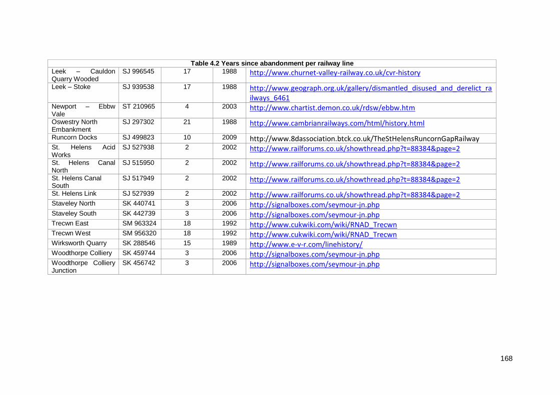
168
Table 4.2 Years since abandonment per railway line
Leek – Cauldon Quarry Wooded
SJ 996545 17 1988 http://www.churnet-valley-railway.co.uk/cvr-history
Leek – Stoke SJ 939538 17 1988 http://www.geograph.org.uk/gallery/dismantled_disused_and_derelict_railways_6461
Newport – Ebbw Vale
ST 210965 4 2003 http://www.chartist.demon.co.uk/rdsw/ebbw.htm
Oswestry North Embankment
SJ 297302 21 1988 http://www.cambrianrailways.com/html/history.html
Runcorn Docks SJ 499823 10 2009 http://www.8dassociation.btck.co.uk/TheStHelensRuncornGapRailway St. Helens Acid Works
SJ 527938 2 2002 http://www.railforums.co.uk/showthread.php?t=88384&page=2
St. Helens Canal North
SJ 515950 2 2002 http://www.railforums.co.uk/showthread.php?t=88384&page=2
St. Helens Canal South
SJ 517949 2 2002 http://www.railforums.co.uk/showthread.php?t=88384&page=2
St. Helens Link SJ 527939 2 2002 http://www.railforums.co.uk/showthread.php?t=88384&page=2 Staveley North SK 440741 3 2006 http://signalboxes.com/seymour-jn.php Staveley South SK 442739 3 2006 http://signalboxes.com/seymour-jn.php Trecwn East SM 963324 18 1992 http://www.cukwiki.com/wiki/RNAD_Trecwn Trecwn West SM 956320 18 1992 http://www.cukwiki.com/wiki/RNAD_Trecwn Wirksworth Quarry SK 288546 15 1989 http://www.e-v-r.com/linehistory/ Woodthorpe Colliery SK 459744 3 2006 http://signalboxes.com/seymour-jn.php Woodthorpe Colliery Junction
SK 456742 3 2006 http://signalboxes.com/seymour-jn.php

169
Figure 4.1. Scatterplot of mean of time since abandonment vs. mean species diversity per relevé per site, showing no relationship between time since abandonment and species diversity
Figure 4.2. Scatterplot of mean of time since abandonment vs. mean species richness per relevé per site, showing no relationship between the two variables

170
Figure 4.3. Scatterplot of mean of time since abandonment vs. mean Ellenberg F values per relevé per site, showing no relationship between time since abandonment and Ellenberg F values
Figure 4.4. Scatterplot of mean of time since abandonment vs. mean Ellenberg N values per relevé per site, showing no relationship between time since abandonment and Ellenberg N values

171
Figure 4.5. Scatterplot of mean of sites vs. mean Ellenberg F values per relevé per site, showing no relationship between the sites and mean Ellenberg F values
Figure 4.6. Scatterplot of mean of sites vs. mean Ellenberg N values per relevé per site, showing no relationship between the sites and Ellenberg N values

172
The lines surveyed show a range of time since abandonment ranging from the
recently closed (e.g. St. Helens Acid Works; 2 years) to those abandoned for
two decades (e.g. the Appleby sites). There is a good range of coverage
between these two extremes. There is no relationship between time since
abandonment and any of Ellenberg N, Ellenberg F, species richness and
species diversity values (Figures 4.1 - 4.6). This outcome does not change,
when data is considered per relevé or a mean value calculated across a site.
The data presented here uses the unweighted values. Using unweighted or
weighted Ellenberg means yields extremely similar results.
CCA and Hierarchical Clustering
Table 4.3 shows mean and standard deviations of time since abandonment,
abiotic and edaphic factors. Superscripts of different letters identify
significantly different mean values between clusters for the same measure.
Absence of letters within a row of means indicates no significant differences.

173
Table 4.3. Mean and standard deviations Cluster A B C D E F G
Indicator species Ep. ciliatum
Eu.
cannabinum
Ar.
elatius
Vu.
bromoides
Li.
vulgaris
Sc.
crassipilum
Fe.
rubra
Ge.
robertianum
Ag.
stolonifera
Ga.
aparine
De.
cespitosa Ur. dioica
Altitude (m)
Mean 170a 30b 70bc 20b 60bc 160a 90c
Standard Deviation 70 10 70 0 0 0 80
Aspect (degrees)
Mean 100ab 90ab 95ab 45a 85ab 140b 105b
Standard Deviation 40 55 50 0 40 50 50
Years since line closure
Mean 14ab 3c 10bc 10abc 3c 20a 14ab
Standard Deviation 4 2 6 0 0 0 12
Mean Rainfall (mm)
Mean 75ab 48c 68b 76ab 69b 80a 61d
Standard Deviation 2 6 7 0 1 0 12
Mean Summer Temp (°C)
Mean 15a 16bcd 16bc 16d 15ac 14e 16bd
Standard Deviation 0 0 1 0 1 0 1
pH
Mean 5.7a 5.5a 5.7a 5.8a 6.2b 5.8a 5.8a
Standard Deviation 0.6 0.4 0.2 0.3 0.4 0.3 0.2
Moisture Content (%)
Mean 0.87a 1.8a 0.92a 3.64a 3.92a 2.23a 2.64a
Standard Deviation 1.22 2.66 1.02 0.33 7.53 0.92 3.77
Organic Content (%)
Mean 18.57ab 13.22ab 18.41ab 14.22ab 52.04c 24.13b 11.97a
Standard Deviation 5.75 8.06 9.85 3.61 12.89 8.71 8.36
Mg (mg/l)
Mean 79.29 74.63 71.42 77.89 50.86 103.96 59.66
Standard Deviation 78.06 65.28 60.96 41.55 19.91 55.22 58.12
Pb (mg/l)
Mean 16.06 84.62 18.09 7.12 6.10 29.97 37.81
Standard Deviation 8.72 86.32 15.50 2.10 4.68 12.01 93.91
K (mg/l)
Mean 19.13 24.99 28.26 15.23 22.47 14.92 21.37
Standard Deviation 9.05 11.32 17.46 4.87 9.01 3.42 8.16
Ca (mg/l)
Mean 56.12a 842.47b 92.61a 112.87a 129.19a 194.76a 213.7a
Standard Deviation 59.38 1416.69 111.99 47.16 101.34 81.67 271.84
Cu (mg/l)
Mean 5.57 17.95 8.50 13.93 12.93 6.06 20.23
Standard Deviation 1.26 8.99 7.81 3.77 20.22 1.25 24.70
Cd (mg/l)
Mean 2.23 1.39 1.35 1.22 6.08 0.45 1.73
Standard Deviation 3.43 0.89 3.51 1.41 21.08 0.17 1.77
Ni (mg/l)
Mean 18.23 14.55 18.95 15.29 17.64 16.62 12.78
Standard Deviation 4.05 11.16 8.57 2.04 2.73 4.15 5.89
ANOVA, used on the various factors examined, reveals some significant
differences between clusters (Table 4.3). For instance, altitude varies from a
mean per cluster of 20m asl to 170m asl with the significantly different
altitudes between clusters; Vulpia bromoides & Galium aparine and
Eupatorium cannabinum & Agrostis stolonifera at significantly lower altitudes

174
with Epilobium ciliatum & Geranium robertianum and Schistidium crassipilum
& Urtica dioica at significantly higher altitude with other clusters at
intermediate altitudes. Aspect shows two significantly different extremes.
Vulpia bromoides and Galium aparine at 45° and Schistidium crassipilum &
Urtica dioica at 140° with the other clusters at intermediate angles. Year since
closure shows two clusters with significantly different early closure dates
(Eupatorium cannabinum & Agrostis stolonifera and Linaria vulgaris &
Deschampsia cespitosa) while the Schistidium crassipilum and Urtica dioica
cluster is significantly oldest. For pH the Linaria vulgaris and Deschampsia
cespitosa cluster has a significantly higher pH than all other clusters. For
some of the factors (altitude, aspect, time since abandonment, mean rainfall
and mean summer temperatures) show no variation, while other samples
show large variance. There is no easily discernible pattern to the significant
differences.
There are no significant differences between the clusters for the majority of
soil characters (moisture content, Mg, Pb, K, Cu, Cd and Ni). Organic content
has significant differences between clusters and Calcium content is
significantly higher in cluster B (Eupatorium cannabinum and Agrostis
stolonifera community) than all others. All other edaphic factors show no
significant differences between clusters.

175
Figure 4.7 CCA of each relevé with rainfall, altitude, time since closure, pH, aspect and summer temperature, showing that rainfall, altitude, summer temperature, aspect and pH are important components
Comparing the climatic factors, time, soil and pH imposes structure on the
biplot. While most sites cluster centrally, the Trecwn sites (TE & TW), are
distinct as are the majority of the Appleby sites (APW, APC & APE). These
are associated with the higher rainfall and altitude vectors (Figure 4.7). These
are important vectors, determined by length of arrow, as are summer
temperature, aspect and pH. Time since closure is of little importance. The
significance of the vectors is considered with Fig 4.9 and Table 4.4 below.

176
Figure 4.8 CCA of each relevé with pH, moisture, organic content and heavy metals, showing that organic content, pH and Magnesium are major components
The soil CCA biplot (Figure 4.8), shows that the major components are
organic content, pH and Magnesium (Mg) content, with the remaining metal
ions and moisture of similar but low impact. Soil characters lead to clustering
of the Trecwn sites (TE & TW) and the St. Helens North relevés (SN) with
some of the St. Helens Canal South relevés (ST.HCANS). Woodthorpe
Colliery Junction (WCJ) and Appleby Cutting (APC) cluster together. The
significance of the vectors is considered with Fig 4.10 and Table 4.5 below.

177
Figure 4.9 CCA of the seven clusters against altitude, aspect, year since abandonment (YearSinceClose), rainfall and summer temperature, showing altitude, aspect, summer temperature and rainfall are significant
Df Chisq F N.Perm Pr(>F)
Altitude 1 0.3304 3.7291 99 0.01 ** Aspect 1 0.2639 2.9784 99 0.01 ** YearSinceClose 1 0.1397 1.5772 99 0.21 Rainfall 1 0.3495 3.9449 99 0.01 ** SummerTemp 1 0.3175 3.5830 99 0.01 ** Residual 168 14.8852 Significance codes: ** p=0.01 No asterisk = NS Table 4.4 Permutation test for CCA plot Fig 4.9 under reduced fit model (Terms added sequentially; first to last).
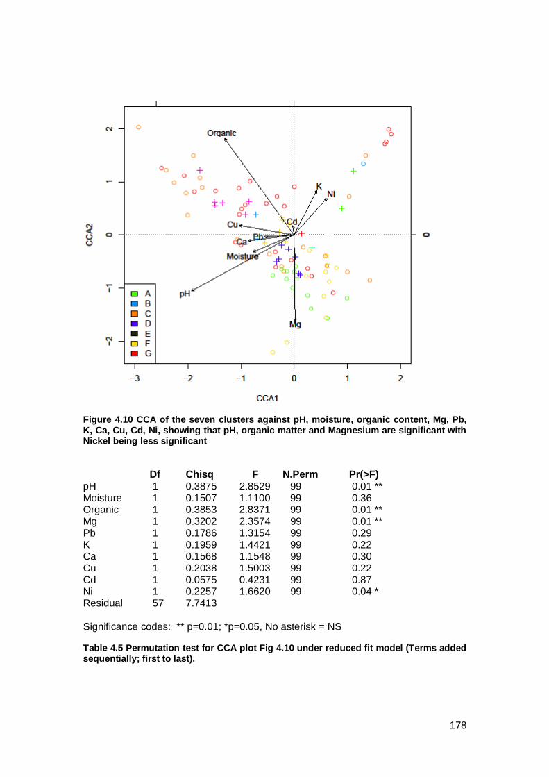
178
Figure 4.10 CCA of the seven clusters against pH, moisture, organic content, Mg, Pb, K, Ca, Cu, Cd, Ni, showing that pH, organic matter and Magnesium are significant with Nickel being less significant
Df Chisq F N.Perm Pr(>F)
pH 1 0.3875 2.8529 99 0.01 ** Moisture 1 0.1507 1.1100 99 0.36 Organic 1 0.3853 2.8371 99 0.01 ** Mg 1 0.3202 2.3574 99 0.01 ** Pb 1 0.1786 1.3154 99 0.29 K 1 0.1959 1.4421 99 0.22 Ca 1 0.1568 1.1548 99 0.30 Cu 1 0.2038 1.5003 99 0.22 Cd 1 0.0575 0.4231 99 0.87 Ni 1 0.2257 1.6620 99 0.04 * Residual 57 7.7413 Significance codes: ** p=0.01; *p=0.05, No asterisk = NS Table 4.5 Permutation test for CCA plot Fig 4.10 under reduced fit model (Terms added sequentially; first to last).

179
When considered as clusters (or communities) rather than individual relevés,
the communities are not randomly distributed within the biplots. Relevés from
the same community, identified by the same colour on the biplots, generally
cluster together, although there is some overlap with adjacent clusters and
towards the centre, while Cluster G is broadly spread. This is seen in both the
abiotic and time since abandonment plot (Figure 4.9) and the soil plot (Figure
4.10), although the soil biplot shows a more diffuse pattern within clusters
than the abiotic values. Statistical analysis of environmental and temporal
CCA shows that altitude, aspect, rainfall and summer temperature are all
significantly associated with the vegetation data. Year since closure is not
associated with the vegetation data. In the soil factors CCA, pH, organic
content, Magnesium content and Nickel content are all significantly associated
with the vegetation separation. All other factors (moisture content, Pb, K, Ca,
Cu and Cd) show no significant relationship with the vegetation data.
Once soil factors, time and abiotic factors are combined in the CCA plot
(Figure 4.11) the abiotic values show a greater impact than the soil factors.
Statistical analysis (Table 4.6) adds time since abandonment to the list of
factors significantly associated with the vegetation data listed above and in
Tables 4.4 and 4.5 (altitude, aspect, rainfall and summer temperature, pH,
organic content, Magnesium content and Nickel content).
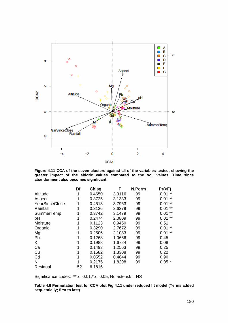
180
Figure 4.11 CCA of the seven clusters against all of the variables tested, showing the greater impact of the abiotic values compared to the soil values. Time since abandonment also becomes significant
Df Chisq F N.Perm Pr(>F)
Altitude 1 0.4650 3.9116 99 0.01 ** Aspect 1 0.3725 3.1333 99 0.01 ** YearSinceClose 1 0.4513 3.7963 99 0.01 ** Rainfall 1 0.3136 2.6379 99 0.01 ** SummerTemp 1 0.3742 3.1479 99 0.01 ** pH 1 0.2474 2.0809 99 0.01 ** Moisture 1 0.1123 0.9450 99 0.51 Organic 1 0.3290 2.7672 99 0.01 ** Mg 1 0.2506 2.1083 99 0.01 ** Pb 1 0.1268 1.0666 99 0.45 K 1 0.1988 1.6724 99 0.08 . Ca 1 0.1493 1.2563 99 0.25 Cu 1 0.1582 1.3308 99 0.22 Cd 1 0.0552 0.4644 99 0.90 Ni 1 0.2175 1.8298 99 0.05 * Residual 52 6.1816 Significance codes: **p= 0.01,*p= 0.05, No asterisk = NS Table 4.6 Permutation test for CCA plot Fig 4.11 under reduced fit model (Terms added sequentially; first to last)

181
4.4 DISCUSSION
Under the traditional model of succession determined by a transition from
extreme tolerant species to competitive types, it is predicted that species
richness and species diversity would both increase over time following
abandonment, before declining as trees begin to dominate, allowing only
shade tolerant species to persist in the ground flora. This view is based upon
studies of pioneer vegetation on other substrates, such as sand dunes (e.g.
Pye et al, 2007). Furthermore as time progresses soil development would
lead to increased nutrient levels resulting in higher Ellenberg N and F scores.
This has not happened in this study. There is no simple temporal pattern with
species richness, species diversity or soil factors. Rather, these all exhibit a
random pattern with respect to time since abandonment. This may be
because the time since abandonment is relatively short. However with these
results it is tempting to consider that succession as studied here is a random
and unpredictable process, where the environmental variables, edaphic
variables and species life strategies are extremely variable and likely to
change in different localities. A view shared by Walker & del Moral (2003) and
Pickett et al (2008). Similar patterns have been found in forest communities
(Wardle et al, 2004), and volcanic communities (del Moral, 2007)) although
these were over a much longer timescale.
However the cluster analysis in the previous chapter revealed some distinct
communities with indicator species significantly associated with them. Hence
it may be appropriate to consider the data at the community level. Significant
differences between communities are revealed in some of the abiotic factors
182
(altitude, aspect, mean rainfall and mean summer temperature). Time for
development is also significantly different as are some edaphic factors (pH,
moisture content, organic content and Ca content), although the majority of
edaphic factors show no significant differences. However while ANOVA is
generally considered a robust statistical tool the markedly unequal variances
in many of the measures mean that the ANOVA results may not be
particularly reliable. Therefore the multivariate analysis is potentially the most
informative.
Multivariate analysis reveals that there are some key factors separating the
communities. These are mainly abiotic (rainfall, summer temperature,
moisture). Soil factors are of less importance, only pH, organic content, Mg
and Ni content are of significance (Fig 4.10). When considered alongside only
abiotic factors time since abandonment is not significant (Fig 4.9). However
when included with soil factors it becomes a significant agent separating the
clusters (Fig 4.11). It is possible that time is an important factor on soil
development. Indeed, on a study of succession on disused coal mines, time
since closure and pH were significant factors affecting the plant community
composition when the substrate had been covered with top-soil. Where no
top-soil is present, the substrate limited succession (Alday et al, 2011). Other
studies have shown mean annual temperature and mean annual rainfall to
affect community composition in arable weed communities, with pH being less
of an significant factor (Cimalová & Lososová, 2009). Similar to this study, a
strong correlation between organic content and pH was discovered during a

183
study of the vegetation communities along an Ethiopian river corridor (Tikssa
et al, 2009).
It is of course possible that not all important architects of community
composition were included in this study. General climatic conditions in an area
have been used in the analysis when specific local conditions may be more
relevant. For instance, the nature of a railway line, whether in a cutting or on
an embankment may influence both climate and seed rain (Vitousek &
Matsom, 1991 and Matlack, 1994). Surrounding land use may also be a factor
in the colonisation of the ballast. Many of the railway lines sampled ran
through rural areas, where permanent pasture was the neighbouring habitat
with little source of seeds. By comparison those sampled in urban areas
where unmanaged rank grassland occurred on the fringes may provide a
more abundant source of propagules.
While there are species significantly associated with the clusters identified in
Chapter three, the associations are not fixed and fidelity and exclusivity are
rarely both strong for any given species. This indicates a random element to
some of the community composition. Nevertheless clustering into distinct
communities does occur and some of this clustering is associated with
particular abiotic and edaphic factors along with time since development. This
implies that given certain conditions there is a predictability to the community
composition. However, no recent ecological work has emerged to support this
view, particularly on synanthropic habitats.

184
CHAPTER 5 – CONSERVATION VALUE AND SUMMARY
5.1 SPECIES AND CONSERVATION VALUE
Across all sites, the study recorded a total of 278 species (including 11 taxa
identified to species level only) (Table 5.1). This includes both vascular plants
and bryophytes.
TABLE 5.1 SPECIES LIST FROM ALL RAILWAY SITES SHOWING THE CONSERVATION DESIGNATION OF EACH SPECIES (JNCC, 2015)
SPECIES CONSERVATION DESIGNATION
Pteridium aquilinum Common
Acer pseudoplatanus Common
Achillea millefolium Common
Agrimonia eupatoria Common
Agrostemma githago Common
Agrostis capillaris Common
Agrostis stolonifera Common
Aira caryophyllea Common
Alliaria petiolata Common
Alnus glutinosa Common
Alnus incana Common
Alopecurus pratensis Common
Amblystegium serpens Common
Anagallis arvensis Common
Angelica sylvestris Common
Anisantha sterilis Common
Anthoxanthum odoratum Common
Anthriscus sylvestris Common
Arabidopsis thaliana Common
Arctium minus Common
Arenaria serpyllifolia Common
Arrhenatherum elatius Common
Artemisia absinthium Common
Artemisia vulgaris Common
Asplenium adiantum-nigrum Common
Asplenium ruta-muraria Common
Asplenium trichomanes Common
Athyrium filix-femina Common
Atrichum undulatum Common
Ballota nigra Common
Barbarea vulgaris Common
Barbula convoluta Common

185
Barbula recurvirostra Common
Barbula unguiculata Common
Bellis perennis Common
Berberis vulgaris Common
Betula pendula Common
Betula pubescens Common
Blackstonia perfoliata Common
Brachypodium sylvaticum Common
Brachythecium rivulare Common
Brachythecium rutabulum Common
Bromus hordeaceus Common
Bryoerythrophyllum recurvirostrum Common
Bryum argenteum Common
Bryum caespiticium Common
Bryum capillare Common
Buddleja davidii Common
Calliergonella cuspidata Common
Calluna vulgaris Common
Calystegia sepium Common
Campylopus introflexus Common
Cardamine flexuosa Common
Cardamine hirsuta Common
Carex flacca Common
Catapodium rigidum Common
Centaurea nigra Common
Centaurium erythraea Common
Cerastium fontanum Common
Cerastium glomeratum Common
Ceratodon purpureus Common
Chaenorhinum minus Common
Chamerion angustifolium Common
Chenopodium polyspermum Common
Cirsium arvense Common
Cirsium palustre Common
Cirsium vulgare Common
Cladeonia sp. Common
Convolvulus arvensis Common
Conyza canadensis Common
Corylus avellana Common
Crataegus monogyna Common
Crepis capillaris Common
Crepis vesicaria Common
Cupressus macrocarpa x Chamaecyparis nootkatensis Common
Cymbalaria muralis Common
Cynosurus cristatus Common
Dactylis glomerata Common
Daucus carota Common

186
Deschampsia cespitosa Common
Deschampsia flexuosa Common
Dicranum scoparium Common
Digitalis purpurea Common
Dipsacus fullonum Common
Dryopteris filix-mas Common
Dyopteris felix-femina Common
Echium vulgare Common
Elytrigia repens Common
Epilobium ciliatum Common
Epilobium hirsutum Common
Epilobium montanum Common
Epilobium palustre Common
Epilobium parviflorum Common
Epilobium sp. Common
Epilobium tetragonum Common
Equisetum arvense Common
Erigeron acer Common
Eupatorium cannabinum Common
Euphrasia officinalis agg. Common
Eurhynchium praelongum Common
Festuca ovina Common
Festuca pratensis Common
Festuca rubra Common
Filipendula ulmaria Common
Fragaria vesca Common
Fraxinus excelsior Common
Galium aparine Common
Galium mollugo Common
Galium palustre Common
Galium parisiense Nationally Scarce
Galium saxatile Common
Galium verum Common
Geranium dissectum Common
Geranium molle Common
Geranium robertianum Common
Geum rivale Common
Geum urbanum Common
Glechoma hederacea Common
Grimmia pulvinata Common
Hedera helix Common
Heracleum sphondylium Common
Hieracium sp. Common
Hieracium umbellatum Common
Holcus lanatus Common
Hypericum humifusum Common
Hypericum montanum IUCN Lower Risk (Near Threatened)

187
Hypericum perforatum Common
Hypericum pulchrum Common
Hypericum tetrapterum Common
Hypnum cupressiforme Common
Hypochaeris radicata Common
Ilex aquifolium Common
Impatiens glandulifera Common
Juncus articulatus Common
Juncus bufonius Common
Juncus effusus Common
Kindbergia praelonga Common
Knautia arvensis Common
Lactuca serriola Common
Lamium album Common
Lamium purpureum Common
Lapsana communis Common
Lathyrus pratensis Common
Laylandii Common
Leontodon autumnalis Common
Leontodon hispidus Common
Leucanthemum vulgare Common
Leycesteria formosa Common
Linaria vulgaris Common
Linum catharticum Common
Lolium perenne Common
Lonicera pericyclamen Common
Lophocolea sp. Common
Lotus corniculatus Common
Luzula campestris Common
Luzula multiflora Common
Luzula sylvatica Common
Lycopus europaeus Common
Matricaria discoidea Common
Medicago lupulina Common
Melilotus officinalis Common
Mercurialis perennis Common
Molinia caerulea Common
Myosotis arvensis Common
Myosotis discolor Common
Nardus stricta Common
Odontites vernus Common
Oenothera biennis Common
Oenothera cambrica Common
Origanum vulgare Common
Pastinaca sativa Common
Peltigera sp. Common
Phalaris arundinacea Common

188
Phleum pratense Common
Picris echioides Common
Pilosella officinarum Common
Pimpinella saxifraga Common
Plantago lanceolata Common
Plantago major Common
Poa annua Common
Poa pratensis Common
Poa pratensis ag. Common
Poa trivialis Common
Polygonum aviculare Common
Polytrichum commune Common
Polytrichum commune v. commune Common
Potentilla erecta Common
Potentilla reptans Common
Potentilla sterilis Common
Primula vulgaris Common
Prunella vulgaris Common
Prunus sp. Common
Pseudocrossidium hornschuchianum Common
Pulicaria dysenterica Common
Quercus robur Common
Racometrium sp. Common
Ranunculus acris Common
Ranunculus bulbosus Common
Ranunculus repens Common
Reseda luteola Common
Rhododendron ponticum Common
Rhytidiadelphus squarrosus Common
Ribes sp. Common
Rosa arvensis Common
Rosa canina Common
Rosa pimpinellifolia Common
Rosa sp. Common
Rosa spinosissima Common
Rubus fruticosus agg. Common
Rubus idaeus Common
Rumex acetosa Common
Rumex acetosella Common
Rumex conglomeratus Common
Rumex crispus Common
Sagina procumbens Common
Salix caprea Common
Salix cinerea Common
Salix sp. Common
Sambucus nigra Common
Sanguisorba minor Common
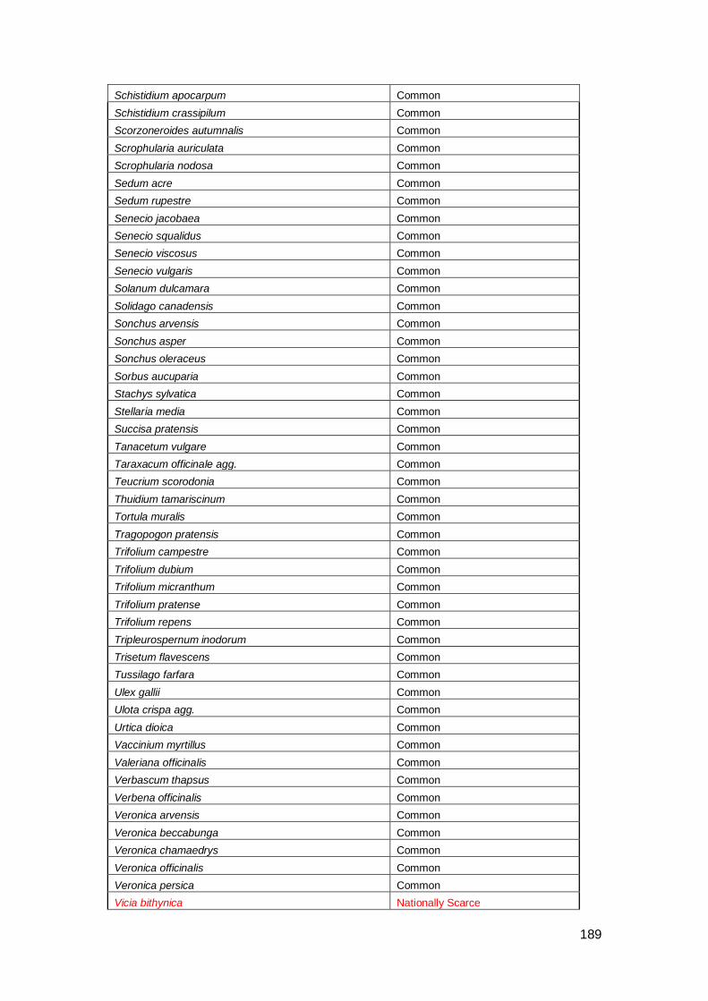
189
Schistidium apocarpum Common
Schistidium crassipilum Common
Scorzoneroides autumnalis Common
Scrophularia auriculata Common
Scrophularia nodosa Common
Sedum acre Common
Sedum rupestre Common
Senecio jacobaea Common
Senecio squalidus Common
Senecio viscosus Common
Senecio vulgaris Common
Solanum dulcamara Common
Solidago canadensis Common
Sonchus arvensis Common
Sonchus asper Common
Sonchus oleraceus Common
Sorbus aucuparia Common
Stachys sylvatica Common
Stellaria media Common
Succisa pratensis Common
Tanacetum vulgare Common
Taraxacum officinale agg. Common
Teucrium scorodonia Common
Thuidium tamariscinum Common
Tortula muralis Common
Tragopogon pratensis Common
Trifolium campestre Common
Trifolium dubium Common
Trifolium micranthum Common
Trifolium pratense Common
Trifolium repens Common
Tripleurospernum inodorum Common
Trisetum flavescens Common
Tussilago farfara Common
Ulex gallii Common
Ulota crispa agg. Common
Urtica dioica Common
Vaccinium myrtillus Common
Valeriana officinalis Common
Verbascum thapsus Common
Verbena officinalis Common
Veronica arvensis Common
Veronica beccabunga Common
Veronica chamaedrys Common
Veronica officinalis Common
Veronica persica Common
Vicia bithynica Nationally Scarce

190
Vicia cracca Common
Vicia hirsuta Common
Vicia orobus Nationally Scarce
Vicia sativa Common
Vicia sepium Common
Vicia tetrasperma Common
Viola arvensis Common
Viola canina IUCN Lower Risk (Near Threatened)
Viola riviniana Common
Viola sp. Common
Vulpia bromoides Common
This list included three species which are classified as Nationally Scarce (taxa
which occur in 26-100 hectads in Great Britain); Galium parisiense, found in
one relevé at St. Helens Canal North; Vicia bithynica, found in one relevé at
Trecwn West and Vicia orobus, found in two relevés at Trecwn West. Two
species classified as IUCN Lower Risk (Near Threatened) were also
recorded; Hypericum montanum, found in two relevés at St. Helens Canal
North and Viola canina, found in one relevé at Cambridge, one relevé at Leek
to Stoke and two relevés at Histon to St.Ives West. IUCN Lower Risk taxa are
based on recent declines in population size and distribution (JNCC). There
were no species recorded at the higher IUCN conservation categories.
Despite the presence of these Nationally Scarce or Near Threatened species
none of the sites would receive statutary conservation protection based upon
the species present.
Specific criteria are used for designating nature conservation sites, such as a
Site of Special Scientific Interest (SSSI) or a Local Wildlife Site (LWS). For
SSSIs a number of parameters are assessed per site, including size,
diverisity, naturalness, rairity, fragility, typicalness and potential value

191
(Ratcliffe, 1977). It is very difficult to apply these critiera to the railway line
sites. For example, rarity could not be used as a criteria as <2% of the total
species found are considered to be rare. Likewise the assemblages at each
site consist of a mix of common species. Hence they would not receive
national legal protection for this reason either.
At a local, non-statutory, level LWS criteria tends to be based on species
assemblages, with a defined number of species required per habitat type to
allow designation. The indicator species are typically of established habitats
such as grassland, woodland etc. Given the assemblages described here are
all ephemeral ruderal communities which rarely feature in LWS criteria, the
assemblages recorded would not lead to protection of any of the sites in this
study. The distinctive community identified in this study; Arrhenatherum
elatius with a ruderal component, which is not documented in any published
statutory and non-statutory guidelines and is likely to be widespread in other
ex-industrial habitats.
5.2 ADDRESSING OF AIMS
This study has focussed on elements of phytosociology using a simple
synanthropic community. It had the following aims.
1. Firstly, to survey and describe plant communities found on disused
railway ballast in the UK, based on floristic data only and using a British
approach (NVC) and to identify any previously undescribed
communities.
192
2. Secondly, to survey and describe the plant communities found using a
the modified Braun-Blanquet method,
3. Thirdly, to analyse the floristic data with environmental, temporal and
edaphic variables as a factor, in an attempt to identify what determines
the community composition and whether communities are random or
can be predicted along a successional process.
4. Finally to consider the potential conservation value of disused railway
lines considering both rare species and species assemblages.
Chapter 1 described the background to phytosociology in Europe, from the
late 19th Century to the present day. The different pathways of ecological
schools of thought were examined, with a discussion on the convergent
thoughts of British ecologists, compared to continental ecologists. Similarly,
gaps in coverage of synanthropic habitat studies were identified. Synanthropic
vegetation has long been studied on the continent but far less frequently
considered in the UK. The NVC has large gaps regarding communities found
on ex-industrial land (Rodwell et al, 2000), whereas databases on the
continent support large numbers of relevés from such habitats and individual
books are published devoted to ruderal plant communities (e.g. Chytrý, 2009).
Railway lines are an easy subject to study. They are linear, constructed in the
same way throughout the UK and time since abandonment is easy to
discover. Likewise other potential abiotic factors. Continental ecologists have
long studied railway vegetation. The UK has few such studies. This work has
filled this gap.

193
Chapter 2 examined the plant communities found on the railway lines by using
the NVC approach. All relevés were sorted into NVC tables and constant
species established. The communities were analysed using MAVIS and by
hand using the NVC publications. Correspondence Analysis was used on the
communities and on typical NVC communities, to find similarities. Few
similarities were found with published NVC communities. A large number of
communities had affinities with MG1 Arrhenatherum elatius grassland but with
un-described sub-communities, with ruderal species as main components or
woody and scrub species as components. Similarly, a number of communities
had affinities to OV communities but with different constant species. It
became clear that it is difficult to apply the NVC to synanthropic habitats and
that there are ruderal communities in existence that are not described in the
NVC. In particular this study identified a new community, that of a
Arrhernatherum elatius community with a sub-community of ruderal species
as main components, with a suggested classification as MG14.
Other NVC communities exhibit a single dominant species across a number of
communities, for example, Quercus woodlands and it is the associated
vegetation and its physiognomy that merit differentiation. Given the
associated species found in this study within the Arrhenatherum elatius
dominated grassland are very different from that described by Rodwell (1992)
for MG1, with short lived ruderal species rather than perennials, and that the
physiognomy is also markedly different, I consider that the community
described here constitutes a new Arrhenatheretum, previously undescribed
from the UK.

194
Chapter 3 utilised a modified Braun-Blanquet approach to analysing the
vegetation data. The Br-Bl method is widely used outside the UK, whereas
within Britain it has rarely been applied. Multivariate analysis revealed no
clear identifiable and separate clusters, however hierarchical cluster analysis
revealed clear splits in the data. Species characteristic of each cluster were
identified using Indicator Values. A total of seven clusters were identified from
the floristic data with distinctive indicator species. The major cluster, is
dominated by Arrhenatherum elatius, with a ruderal component and a lack of
umbellifers. A large set of clusters had strong ruderal components or woody
components, which is similar to the NVC findings.
Chapter 4 investigated the potential contribution of environmental, temporal
and edaphic variables on each of the sites and clusters identified in the
previous chapter. This was underpinned by a theoretical question as to the
nature of vegetation dynamics. Successional processes have long been
presented as simple temporal progression as one group of species replaces
another based upon the characteristics of the species, for instance ruderal
through to biannual and perennial forbs and grasses ending in a tree
dominated climax community. The more modern approach is to view the
process as much more stochastic. The synanthropic communities here which
are of varying ages represent a unique opportunity to address this question.
Are the predominantly ruderal communities identified here a random
amalgamation of plants or as a series of predictable successional
communities determined by temporal, abiotic and edaphic factors.

195
A number of factors potentially influencing community composition were
incorporated into the study. These included abiotic factors; summer
temperature, rainfall, altitude and aspect and edaphic factors; pH, moisture
content, organic content, metal ion content and time since abandonment. Soil
nutrient level was also investigated using Ellenberg indicator values. Simple
investigation of the impact of time on species richness, diversity and soil
nutrient level revealed no relationship either at the individual relevé or at the
clusters identified in the previous chapter. CCA analysis was more revealing
showing that rainfall, summer temperature and moisture were an important
part of community composition with soil factors such as Lead and Potassium
having no significant impact. Time since abandonment only becomes
significant when it is combined with soil factors. This suggests that community
composition is not entirely random in these communities. No similar studies
have been undertaken which address the nature of early successional
processes in synanthropic habitats. Thus this study is a significant
contribution to the literature.
Chapter five above highlighted that there is little chance of these sites being
protected by conservation legislation, although the value of such sites to
pollinators with their long flowering season and to other invertebrates with
their lack of disturbance is recognised.

196
5.3 FURTHER WORK
The major findings of this study are the discovery of new plant communities
within the UK and an understanding of successional processes on
synanthropic habits. Several lines of further work then develop from these
discoveries. These suggestions would all be original contributios to the
literature.
1. To revisit extant disused lines and to repeat the survey undertaken
here, thus revealing the nature of temporal changes at particular sites.
This would contribute to understanding the nature of succession at
synanthropic sites.
2. To describe and analyse the vegetation at different synanthropic
habitats, particularly other ex-industrial sites. This would identify
whether the communities identified in chapter three are more
widespread or restricted to disused railway lines. Thus to determine the
extent of the additional communities described herein.
3. In addition, ex-industrial sites have potential value for invertebrate
communities. Through observations undertaken during this study and
professional experience elsewhere hymenoptera and coleoptera are
regularly observed. It would be worthwhile investigating the
invertebrate communities and the ecological principles that underpin
them within these habitats.
197
REFERENCES
Alday, J. G., Marrs, R. H. & Martínez-Ruiz, C. (2011). Vegetation succession on reclaimed coal wastes in Spain: the influence of soil and environmental factors. Applied Vegetation Science, 14, 64-94.
Almquist, E. (1957). Järnvägsfloristiska notiser. Svensk. Bot. Tidskr., 51, 1, 223-263. Angiolini, C., Bacchetta, G, Brullo, S, Casti, M, Giusso del Galdo, G & Guarino, R. (2005). The vegetation of mining dumps in SW-Sardinia. Feddes Repertorium, 116, 3–4, 243–276. Averis, A., Averis, B., Birks, J., Horsfeld, D., Thompson, D. & Yeo, M. (2004). An Illustrated Guide to British Upland Vegetation. JNCC. Baker, S. K. (2004). Rail Atlas Great Britain and Ireland 10th Ed. Oxford Publishing Company. Baker, S. K. (2010). Rail Atlas Great Britain and Ireland 12th Ed. Oxford Publishing Company. Barkman, J. J. (1989). Fidelity and character species; a critical evaluation. Vegetatio, 85, 105-116. Becking, R. (1957). The Zurich-Montpelier school of phytosociology. Bot. Rev. 23, 411-488. Bell, L. C. (2001). Establishment of native ecosystems after mining – Australian experience across diverse geographic zones. Eco. Engineering, 17, 179-186. Biondi, E. & Casavechia, S. (2001). Phytosociological survey of North California dunes. Plant Biosystems, 135 (3), 351-362. Blake, S., McCracken, D. I., Eyre, M. D., Garside, A. & Foster, G. N. (2003). The relationship between the classification of British ground beetle assemblages (Coleoptera, Carabidae) and the National Vegetation Classification of British plant communities. Ecography, 26, 5, 602-616. Bonte, L. (1930). Beitrage zur adventiveflora des rheinisch-Westfalischen industriegebietes. Verh. Naturhist. Vereines. Preuss. Rheinl. Westfalens., 86, 141-255. Bradshaw, A. D. (1970). Plants and industrial waste. Trans. Bot. Soc. Edinburgh, 41, 71-84. Brandes, D. (1979). Bahnöfe als Untersuchungsobjekte der Geo-botanik. Mitt. Tech. Univ. Carola-Wilhelmina, Braunschweig., 14 (314), 49-59.

198
Brandes, D. (1983). Flora und vegetation der bahnhöfe mittel Europas. Phytocoenologia, 11 (1), 31-115. Braun-Blanquet, J. (1915) Les Cévennes méridionales (massif de l'Aigoual). Études sur la végétation méditteranéenne. I. Arch. Sci. Phys. Nat. 48. Braun-Blanquet, J. (1928). Pflanzensoziologie Grundzüge der Vegetationskunde. Springer, Berlin. Braun-Blanquet, J. (1931) L'importance pratique de la sociologie végétale. Comm. Stat. Intern. Géobot. Médit. Alp. 4. Braun-Blanquet, J. (1932). Plant Sociology; the study of plant communities (English Translation). McGraw-Hill, New York. Bruelheide, H. (2000). A new measure of fidelity and its application to defining species groups. Journal of Vegetation Science, 11, 167-178. Caccianiga, M., Luzzaro, A., Pierce, S., Ceriani, R. M. & Cerabolini, B. (2006). The functional basis of a primary succession resolved by CSR classification. Oikos, 112 (1), 10-20. Chapin, F. S., Walker, L. R., Fastie, C. L. & Sharman, L. C. (1994). Mechanisms of Primary Succession Following Deglaciation at Glacier Bay, Alaska. Ecological Monographs, 64 (2), 149-175. Chytrý, M. & Opýpková, Z. (2003). Plot sizes used for phytosociological sampling of European vegetation. Journal of Vegetation Science, 14, 563-570. Chytry, M. & Tichy, L. (2003). Diagnostic, constant and dominant species of vegetation classes and alliances of the Czech Republic: a statistical revision. Folia Fac. Sci. Nat. Univ. Masaryk Brun. Biol.,108, 1-231. Cimalová, S. & Lososová, Z. (2009). Arable weed vegetation of the north-eastern part of the Czech Republic: effects of environmental factors on species composition. Plant Ecology, 203, 45-57. Claisse, P. A. & Calla, C. (2006). Rail ballast: conclusions from a historical perspective. Proceedings from the ICE – Transport, volume 159, 2, 69-74. Clark, R. K. & Clark, S. C. (1981). Floristic diversity in relation to soil characteristics in a lead mining complex in the Pennines, England. New Phytol., 87, 799-815. Clements, F. E. (1905). Research Methods in Ecology. Univ. Publ. Lincoln. Clements, F. E. (1916). Plant succession: an analysis of the development of vegetation. Carnegie Inst. Wash. Publ., 242.
199
Clements, F. E. (1936). Nature and structure of the climax. Journal of Ecology, 24, 254-282. Crowe, T. M. (1979). Lots of weeds: insular phytogeography of vacant urban lots. Journal of Biogeography, 6, 169-181. David, R. W. (2013). labdsv: Ordination and Multivariate Analysis for Ecology. R package version 1.6-1. (http://cran.r-project.org/web/packages/labdsv/labdsv.pdf). de Caceres, M. & Legendre, P. (2009). Associations between species and groups of sites: indices and statistical inference. Ecology, 90, 3566–3574. de Mendiburu, F. (2014). agricolae: Statistical Procedures for Agricultural Research. R package version 1.2-1. http://CRAN.R-project.org/package=agricolae del Moral, R. (2007). Limits to convergence of vegetation during early primary succession. Journal of Vegetation Science, 18, 479-488. Dettmar, J. (1992). Industrietypische flora und vegetation im Ruhrgebiet. Dissertationes Botanicae 191, Cramer, Berlin. Dony, J. G. (1955). Notes on the Bedfordshire railway flora. Beds. Naturalist, 9, 12-16. Dony, J. G. (1974). Some problems of a railway flora. In: Research and Management in Wildlife Conservation 2. Herts. & Middx. Trust Symposium No. 2. Duckworth, J. C., Kent, M. & Ramsey, P. M. (2000). Plant functional types: an alternative to taxonomic plant community descriptions in biogeography? Progress in Physical Geography, 24, 515-542. Dufrêne, M and Legendre, P. (1997). Species assemblages and indicator species: the need for a flexible asymmetrical approach. Ecological Monographs 67: 345-366. Ellenberg, H. (1988). Vegetation Ecology of Central Europe, 4th Edn. Cambridge University Press. Evans, F. C. & Dahl, E. (1955). The vegetational structure of an abandoned field in south-eastern Michigan and its relation to environmental factors. Ecology, 36, 685-706. Favero-longo, S. E., Siniscalco, C. & Piervittori, R. (2006). Plant and lichen colonization in an asbestos mine: Spontaneous bioattenuation limits air dispersion of fibres. Plant Biosystems, 140, 2, 190-205.

200
Flauhault, C. (1901). A project of phytogeographic nomenclature. Bull. Torrey. Bot. Club, 28, 391-409. Galili, T. (2014). dendextend: Extending R's dendrogram functionality. R package version 0.16.1. Gentili, R., Sgorbati, S. & Baroni, C. (2011). Plant species patterns and restoration perspectives in the highly disturbed environment of the Carrara marble quarries (Apuan Alps, Italy). Restoration Ecology, 19 (101), 32-42. Gleason, H. A. (1917). The structure and development of the plant association. Bull. Torrey Bot. Club, 44, 463-481. Gleason, H. A. (1926). The individualistic concept of the plant association. Bull. Torrey. Bot. Club, 53, 7-26. Grime, J. P. (2001). Plant Strategies, Vegetation Processes and Ecosystem Properties (2nd Edn.), John Wiley & Sons Limited, Chichester. Grime, J. P., Hodgson, J. G. & Hunt, R. (1988). Comparative Plant Ecology. A Functional Approach to Common British Species. London: Unwin Hyman. Gutte, P. (1972). Ruderalpflanzengesselschaften West und Mittelsachsens. Feddes Repert., 83, 11-122. Hall, I. G. (1959). The ecology of disused pit heaps in England. Journal of Ecology, 45 (3), 689-720. Hamzehée, B., Naqinezhad, A., Attar, F., Ghahreman, A., Assadi, M. & Prieditis, N. (2008). Phytosociological survey of remnant Alnus glutinosa ssp. barbata communities in the lowland Caspian forests of Northern Iran. Phytocoenologia, 38, 1-2, 117-132. Hepburn, I. (1942). The vegetation of the Barnack stone quarries. Journal of Ecology, 30, 57-64. Hiller, D.A. (2000). Properties of urbic Anthrosols from an abandoned shunting yard in the Ruhr area, Germany. Catena, 39 (4), 245-266. Hodge, S. J. & Harmer, R. (1996). Woody colonization on unmanaged urban and ex-industrial sites. Forestry, 69 (3), 245-261. Holler, A. (1883). Die eisenbahn als verbreitungsmittel von pflanzen. Flora, Jena, 66, 197-205. Hughes, M. R., Colston, A. & Mountford, J. O. (2005). Restoring riparian
ecosystems: The challenge of accommodating variability and designing restoration trajectories. Ecology and Society, 10, 1, Article: 12.

201
Humboldt, A. von. (1805). Essai sur la Géographie des Plante: accompagne d’un tableau physique des regions equinoxiales. Levrault, Paris. Husson, F., Josse, J., Le, S. & Mazet, J. (2014). FactoMineR: Multivariate Exploratory Data Analysis and Data Mining with R. R package version 1.27. http://cran.r-project.org/web/packages/FactoMineR/FactoMineR.pdf Jochimsen, M. E. (2001). Vegetation development and species assemblages in a long-term reclamation project on mine spoil. Eco. Engineering, 17, 187-198. Kent, M. & Coker, P. (1992). Vegetation Description and Analysis: A Practical Approach. Belhaven. Kent, M. (2013). Vegetation Description and Data Analysis - A Practical Approach, Second edition. Oxford University Press. (http://cran.r-project.org/web/packages/indicspecies/indicspecies.pdf). Kimmerer, R. W. (1984). Vegetation development on a dates series of abandoned lean and zinc mines in Southern Wisconsin. The American Midland Naturalist, 111, 332-341. Knapp, R. (1961). Vegetations-Einheiten der Wegränder und der Eisenbahn-Anlagen in Hessen und im Bereich des unteren Neckar. Ber. Oberhess. Ges. Natur-Heilk. Giessen-Naturwiss. Abt., N.F., 31, 122-154. Knollová, I., Chytrý, M., Tichý, L. & Hájek, O. (2006). Local ranges of phytosociological associations: are they reflected in numerical classification? Biologia, Bratislava, 61 (1), 71-77. Kopecký, K. & Hejny, S. (1974). A new approach to the classification of anthropogenic plant communities. Vegetatio, 29, 17-20. Kreh, W. (1960). Die pflanzenwelt des Güterbahnhofs in ihrer Abhängigkeit von Technik und verkehr. Mitt. Florist. Soziol. Arbeitsgem. N.F., 8, 86-109. Kreuzpointner, J. B. (1876). Notizen zur flora Munchens. Flora, Jena, 59, 77-80. Lanta, V. & Leps, J. (2009). How does surrounding vegetation affect the course of succession: A five-year container experiment. Journal of Vegetation Science, 20 (4), 686-694. Large, A. R. G., Mayes, W. M., Newson, M. D. & Parkin, G. (2007). Using long-term monitoring of fen hydrology and vegetation to underpin wetland restoration strategies. Applied Vegetation Science, 10, 3, 417-428. Lasić, A., Jasprica, N., Morovíc, M., Kapetanović, T., Carić, M., Drešković, N., Glavić, N. & Mitić, B. (2014). Biologia, 69 (1), 40-52.

202
Lee, J. A. & Greenwood, B. (1976). The colonisation by plants of calcareous wastes from the salts and alkali industry in Cheshire, England. Biol. Cons., 10, 131-149. Lehman, E. (1895). Flora von polnisch-livland. Arch. Naturk. Liv-Ehst-Kurlands. (Ser. 2). Biol. Naturk. II. 1-422. Lejmbach, B., Rurka, Z., Siedkecjka, B. & Sijka, J. (1965). The flora of the railway tracks of the Eastern Pomeranian coast. Fragm. Flor. Geobot., 21, 53-66. Lienenbecker, H. & Raabe, U. (1981). Vegetation auf bahnhöfen des ost-Munsterlandes. Ber. Naturw. Ver. Bielefeld., 25, 129-141. Lockton, A. & Whild, S. (2014). The Flora of Shropshire. Shropshire Botanical Society. Lososová, Z. & Simonová, D. (2008). Changes during the 20th century in species composition of synanthropic vegetation in Moravia (Czech Republic). Preslia, 80, 291-305. Lososová, Z., Chytrý, M., Cimalová, S., Otýpková, Z., Pyšek, P. & Tichý, L. (2006). Classification of weed vegetation of arable land in the Czech Republic and Slovakia. Folia Geobotanica, 41, 259-273. Lund, A. C. (1974). Analysis of urban plant communities of Atlanta, Georgia. Ph.D. Thesis, Emory Univ., Atlanta, Georgia, USA. Malawska, M. & Wilkomirski, B. (2000). An analysis of soil and plant (Taraxacum officinale) contamination with heavy metals and polycyclic aromatic hydrocarbons (PAHs) in the area of the railway junction Ilana Glowna, Poland. Water, Air and Soil Pollution, 217, 339-349. Matlack, G. R. (1994). Plant species migration in a mixed-history forest landscape in eastern North America. Ecology, 7, 1491-1502. McLaughlin, B. E. & Crowder, A. A. (1988). The distribution of Agrostis gigantea and Poa pratensis in relation to some environmental factors on a
mine-tailings area at Copper Cliff, Ontario. Canadian Journal of Botany, 66 (11), 2317-2322. McVean, D. N. & Ratcliffe, D. A. (1962). Plant Communities of the Scottish Highlands. H.M.S.O., London. Messenger, K. G. (1968). A railway flora of Rutland. Proc. Bot. Sot. Brit. Isl., 7, 325-344. Mikkola, R. (1966). Ratakasvihavaintoja siitaman ja Lylyn seudulta (orivesi, Kangasala ja Juupajoki, Ta). Memoranda. Soc. Fauna Flora Fenn, 42, 14-26.

203
Mirkin, B. M. & Naumova, L.G. (2009). Braun-Blanquet method of vegetation classification in Russia. Zhurnal Obshchei Biologii, 70, 1, 66-77. Moss, C. E. (1910). The fundamental units of vegetation. New Phytol., 9, 18-53. Mucina, L., Grabherr, G. & Ellmauer, T. (1993). Die Pflanzengesellschaften Osterreichs – Teil I. Anthropogene Vegetation, Stuttgart: Fisher. Muehlenbach, V. (1979). Contributions to the synanthropic (adventives) flora of the railroads in St. Louis, Missouri, USA. Ann. Mo. Bot. Gdn., 66, 1-108. Niemi, A. (1969). On the railway vegetation and flora between Esbo and Inga, south Finland. Acta. Bot. Fenn., 83, 1-28. Nowak, A., Nowak, S., Nobis, M. & Nobis, A. (2014a). Vegetation of rock clefts and ledges in the Pamir Alai Mts, Tajikistan (Middle Asia). Cent. Eur. J. Biol., 9 (4), 444-460. Nowak, S., Nowak, A., Nobis, M. & Nobis, A. (2014b). Caucalido platycarpi-Vicietum michauxii − a new weed association from crop fields of Kyrgyzstan (Middle Asia). Cent. Eur. J. Biol., 9 (2), 189-199. Oksanen, J., Guillaume Blanchet, F., Kindt, R., Legendre, P., Minchin, P. R., O'Hara, R. B., Simpson, G. L., Solymos, P.M., Stevens, H. H. & Wagner, H. (2013) vegan: Community Ecology Package. R package version 2.0-10. (http://CRAN.R-project.org/package=vegan) Passarge, H. (1957). Zur soziologischen stellung einiger bahnbegleitender Neophyten in der Mark Brandenburg. Mitt. For-soz. Arbeitsgem. N. F., 6 (7), 155-163. Pedersen, A. (1955). Indslaebte planter ved jernbanerne. Flora og Fauna, 61, 81-109. Peinado, M., Aguirre, J. L., Delgadillo, J. & Martínez-Parras, J. M. (2005a). A phytosociological survey of the chionophilous communities of western North America. Part I: temperate and Mediterranean associations. Plant Ecology, 180, 187-241. Peinado, M., Aguirre, J. L., Delgadillo, J. González, J. & Martínez-Parras, J. M. (2005b). A phytosociological survey of the chionophilous communities of western North America. Part II: boreal associations. Plant Ecology, 180, 243-256. Pfitzenmeyer, C. D. C. (1962). Biological flora of the British Isles: Arrhenatherum elatius. Journal of Ecology, 50 (1), 235-245.

204
Pickett, S. T. A., Cadenasso, M. L. & Meiners, S. J. (2008). Ever since Clements: from succession to vegetation dynamics and understanding to intervention. Applied Vegetation Science, 12, 9-21. Poore, M. E. D. & McVean, D. N. (1957). A new approach to Scottish mountain vegetation. Journal of Ecology, 45, 401-439. Poore, M. E. D. (1955a). The use of phytosociological methods in ecological investigations. I: The Braun-Blanquet system. Journal of Ecology, 43, 226-244. Poore, M. E. D. (1955b). The use of phytosociological methods in ecological investigations. II: Practical issues involved in an attempt to apply the Braun-Blanquet system. Journal of Ecology, 43, 245-269. Poore, M. E. D. (1955c). The use of phytosociological methods in ecological investigations. III: Practical application. Journal of Ecology, 43, 606-651. Poore, M. E. D. (1956). The use of phytosociological methods in ecological investigations IV: General discussion of phytosociological problems. Journal of Ecology, 44, 28-50. Pott, R. (1992). Die Pflanzengesellschaften Deutschlands. Ulmer, Stuttgart. Prach. K., Lencová, K., Řehounková, K., Dvořáková, H., Jírová, A., Konvalinková, P., Mudrák, O., Novák, J. & Trnková, R. (2013). Spontaneous vegetation succession at different central European mining sites: a comparison across seres. Environmental Science and Pollution Research, 20 (11), 7680-7685. Pye, K., Saye, S. E. & Blott, S. J. (2007). Sand Dune Processes and Management for Flood and Coastal Defence. Part 3. The Geomorphological and Management Status of Coastal Dunes in England and Wales. R & D Technical Report FD 1302/TR. DEFRA, London, 94pp. Ranwell, D. (1960). Newborough Warren, Anglesey: II. Plant Associes and Succession Cycles of the Sand Dune and Dune Slack Vegetation. Journal of Ecology, 48 (1), 117-141. Ratcliffe, D. A. (1977). A Nature Conservation Review. Cambridge University Press. Raunkiaer, C. (1934). The Life Forms of Plants and Statistical Plant Geography. Oxford. Repp, G. (1958). Die unkraut vegetation auf Bahnkörpern im Hinblick auf die Bekämpfung mit herbiziden Wuchsstofen. Angew. Bot., 32, 91-104. Roberts, R. D., Marrs, R. H., Skeffington, R. A. & Bradshaw, A. D. (1981). Ecosystem development on naturally colonised china clay wastes 1:

205
Vegetation changes and overall accumulation of organic matter and nutrients. Journal of Ecology, 69, 153-161. Rodwell, J. S. (1991-2000). British Plant Communities, Volumes I – V. Cambridge Univ. Press. Rodwell, J. S., Dring, J. C., Averis, A. B. G., Proctor, M. C. F., Malloch, A. J. C., Schaminée, J. N. J. & Dargie, T. C. D. (2000). Review of coverage of the National Vegetation Classification. JNCC Report, No. 302. Sargent, C. (1984). Britain’s Railway Vegetation. Natural Environment Research Council. The Cambrian News, Aberystwyth. Shaw, P. J. A. (1990). The ecology and conservation potential of PFA and other alkaline wastes. Memorandum from Conference, Hatfield Polytechnic, May 1990. Shaw, P. J. A. (1992). A preliminary study of successional changes in vegetation and soil development on unamended fly ash (PFA) in southern England. Journal of Applied Ecology, 29, 728-736. Shimwell, D. W. (1968). The Phytosociology of calcareous grasslands in the British Isles. Ph.D. Thesis, Univ. of Durham. Shimwell, D. W. (1971). The Description and Classification of Vegetation. Sidgwick & Jackson, London. Šilc, U. & Košir, P. (2006). Synanthropic vegetation of the city of Kranj (Central Slovenia). Hacquetia, 5 (1), 213-231. Silverside, A. J. (1977). A phytosociological survey of British arable weeds and related communities. Ph.D. Thesis, Univ. of Durham. Simonová, D. (2008). Vegetation of trampled habitats in the Czech Republic: a formalised phytosociological classification. Phytocoenologia, 38 (3), 177-191. Smith, A. J. E. (2004). The Moss Flora of Britain and Ireland. Cambridge University Press. Stace, C. A. (2010). New Flora of the British Isles, 3rd Ed. Cambridge University Press. Sukopp, H. & Werner, P. (1983). Urban environments and vegetation. In Man's Impact on Vegetation (eds. Holzner, W., Werger, M. J. A. & Ikusima, I.). W. Junk, The Hague, Netherlands, pp. 247-260. Sukopp, H., Hejny, S. & Kowarik, I. (eds.) (1990). Urban Ecology: Plants and Plant Communities in Urban Environments. SPB Academic Publishing, The Hague, The Netherlands.

206
Suominen, J. (1969). The vegetation of railway yards and adjacent storage areas in Finland. Ann. Bot. Fenn., 6, 353-367. Svenning, J. & Skov, F. (2007). Ice age legacies in the geographical distribution of tree species richness in Europe. Global Ecology and Biogeography, 16 (2), 234-245. Tansley, A. G. (1904). The problems of ecology. New Phytol., 3, 191-200. Tansley, A. G. (1939). The British Isles and their Vegetation. Cambridge Univ. Press. Tichy, L. (2002). JUICE, software for vegetation classification. J. Veg. Sci., 13, 451-453. Tikssa, M., Bekele, T. & Kelbessa, E. (2009). Plant community distribution and variation along the Awash river corridor in the main Ethiopian rift. African Journal of Ecology, 48, 21-28. Turner, W. R., Nakamura, T. & Dinetti, M. (2004). Global urbanisation and the separation of humans from nature. BioScience, 54, 585-590. Tuxen, R. (1955). Das System der nordwestdeutschen Pflanzengesellschaften. Mitteilungen der Florist-soziologischen Arbeitsgemeinschaft, N. F. 5, 155-176. van der Maarel, E., Boot, R., van Dorp, D. & Rijntjes, J. (1985). Vegetation succession on the dunes near Oostvoorne, the Netherlands, a comparison of the vegetation in 1959 and 1980. Vegetatio, 58, 137-187. Vitousek, P. M. & Matson, P.A. (1991). Gradient analysis of ecosystems. In: Cole, J., Lovett, G. M. & Findlay, S. (eds.). Comparative analyses of ecosystems: patterns, mechanisms and theories. pp. 287-298. Springer-Verlag, New York. Walker, L. R. & del Moral, R. (2003), Primary Succession and Ecosystem Rehabilitation, Cambridge University Press, Cambridge. Walker, L. R. (2012). The Biology of Disturbed Habitats. Oxford University Press, Oxford. Wardle, D. A., Walker, L. R. & Bardgett, R. D. (2004). Eco-system properties and forest decline in contrasting long-term chronosequences. Science, 305, 509-523. Werger, M. J. A. (1973). On the use of association-analysis and principal components analysis in interpreting a Braun-Blanquet phytosociological table of a Dutch grassland. Vegetatio, 28, 129-144.

207
Williams, J. T. & Varley, Y. W. (1967). Phytosociological studies of some British grasslands. Vegetatio, 15, 169-189. Willner, W., Di Pietro, R. & Bergmeier, E. (2009). Phytogeographical evidence for post-glacial dispersal limitation of European beech forest species. Ecography, 32 (6), 1011-1018. Wright, A. & Wheater, C. P. (1993). Aspects of the vegetation of an area of disused railway line in Derbyshire. Sorby Record, 30, 57-67. (http://cran.r-project.org/web/packages/dendextend/dendextend.pdf)

APPENDIX 1 - RAW DATA – ON ATTACHED DISK
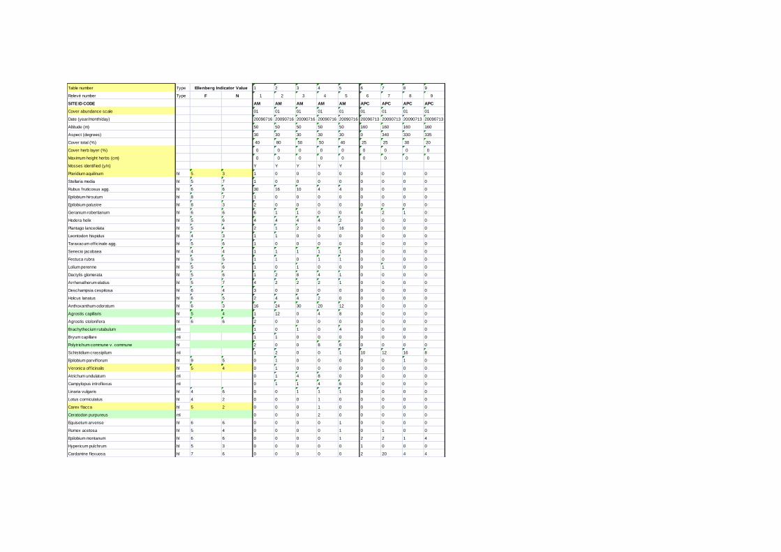
Table number Type 1 2 3 4 5 6 7 8 9
Relevé number Type F N 1 2 3 4 5 6 7 8 9
SITE ID CODE AM AM AM AM AM APC APC APC APC
Cover abundance scale 01 01 01 01 01 01 01 01 01
Date (year/month/day) 20090716 20090716 20090716 20090716 20090716 20090713 20090713 20090713 20090713
Altitude (m) 50 50 50 50 50 160 160 160 160
Aspect (degrees) 30 30 30 30 30 0 340 330 335
Cover total (%) 40 80 50 50 40 25 25 30 20
Cover herb layer (%) 0 0 0 0 0 0 0 0 0
Maximum height herbs (cm) 0 0 0 0 0 0 0 0 0
Mosses identif ied (y/n) Y Y Y Y Y
Pteridium aquilinum hl 5 3 1 0 0 0 0 0 0 0 0
Stellaria media hl 5 7 1 0 0 0 0 0 0 0 0
Rubus fruticosus agg. hl 6 6 30 16 10 4 4 0 0 0 0
Epilobium hirsutum hl 8 7 1 0 0 0 0 0 0 0 0
Epilobium palustre hl 8 3 2 0 0 0 0 0 0 0 0
Geranium robertianum hl 6 6 6 1 1 0 0 4 2 1 0
Hedera helix hl 5 6 4 4 4 4 2 0 0 0 0
Plantago lanceolata hl 5 4 2 1 2 0 16 0 0 0 0
Leontodon hispidus hl 4 3 1 1 0 0 0 0 0 0 0
Taraxacum off icinale agg. hl 5 6 1 0 0 0 0 0 0 0 0
Senecio jacobaea hl 4 4 1 1 1 1 1 0 0 0 0
Festuca rubra hl 5 5 1 1 0 1 1 0 0 0 0
Lolium perenne hl 5 6 1 0 1 0 0 0 1 0 0
Dactylis glomerata hl 5 6 1 2 8 4 1 0 0 0 0
Arrhenatherum elatius hl 5 7 4 2 2 2 1 0 0 0 0
Deschampsia cespitosa hl 6 4 3 0 0 0 0 0 0 0 0
Holcus lanatus hl 6 5 2 4 4 2 0 0 0 0 0
Anthoxanthum odoratum hl 6 3 16 24 30 20 12 0 0 0 0
Agrostis capillaris hl 5 4 1 12 0 4 8 0 0 0 0
Agrostis stolonifera hl 6 6 2 0 0 0 0 0 0 0 0
Brachythecium rutabulum ml 1 0 1 0 4 0 0 0 0
Bryum capillare ml 1 1 0 0 0 0 0 0 0
Polytrichum commune v. commune hl 2 0 0 8 6 0 0 0 0
Schistidium crassipilum ml 1 2 0 0 1 10 12 16 8
Epilobium parvif lorum hl 9 5 0 1 0 0 0 0 0 1 0
Veronica off icinalis hl 5 4 0 1 0 0 0 0 0 0 0
Atrichum undulatum ml 0 1 4 8 0 0 0 0 0
Campylopus introflexus ml 0 1 1 4 6 0 0 0 0
Linaria vulgaris hl 4 6 0 0 1 1 1 0 0 0 0
Lotus corniculatus hl 4 2 0 0 0 1 0 0 0 0 0
Carex f lacca hl 5 2 0 0 0 1 0 0 0 0 0
Ceratodon purpureus ml 0 0 0 2 0 0 0 0 0
Equisetum arvense hl 6 6 0 0 0 0 1 0 0 0 0
Rumex acetosa hl 5 4 0 0 0 0 1 0 1 0 0
Epilobium montanum hl 6 6 0 0 0 0 1 2 2 1 4
Hypericum pulchrum hl 5 3 0 0 0 0 0 1 0 0 0
Cardamine f lexuosa hl 7 6 0 0 0 0 0 2 20 4 4
Ellenberg Indicator Value

APPENDIX 2 - R CODING
#Code for analysis of vegetation data from disused railway lines #28/02/14 #Robert Ashton #Set working directory and import data and check it has been imported correctly setwd("C:\\RFiles\\RailTrack\\PCA\\") railData = read.csv(file = "ImportData.csv", stringsAsFactors = FALSE, header = TRUE, sep = ",", row.names = 1) names(railData) str(railData) #Convert to matrix for use in metaMDS mdsData = data.matrix(railData) str(mdsData) names(mdsData) ##Use vegan package library(vegan) #Perform NMDS rail_NMDS = metaMDS(comm = mdsData, k = 2, trymax = 100, autotransform = FALSE) #Sheperd Plot pdf("sheperdplot.pdf") stressplot(rail_NMDS) dev.off() #Removes numbers from row titles of railData for use in colouring colUse = as.factor(gsub("\\d", "", row.names(railData))) colCodes = c("#000000", "#FFFF00", "#1CE6FF", "#FF34FF", "#FF4A46", "#008941", "#006FA6", "#A30059", "#FFDBE5", "#7A4900", "#0000A6", "#63FFAC", "#B79762", "#004D43", "#8FB0FF", "#997D87", "#5A0007", "#809693", "#FF0800", "#1B4400", "#4FC601", "#3B5DFF", "#4A3B53", "#FF2F80", "#61615A", "#BA0900", "#6B7900", "#00C2A0", "#FFAA92", "#FF90C9", "#B903AA", "#D16100", "#DDEFFF", "#000035", "#7B4F4B") colCodes2 = rainbow(35) colVec = colCodes[colUse] #Scatter plots pdf("sitesplot.pdf") plot(rail_NMDS, display = "sites") orditorp(rail_NMDS, display = "sites", col = colCodes[colUse], pch = 19, labels = FALSE) legend("topleft", legend = levels(colUse), fill = colCodes, cex = 0.69) dev.off() pdf("speciesplot.pdf") plot(rail_NMDS, display = "species") dev.off()

#PCA code #Load FactoMineR package library(FactoMineR) #Conduct PCA pca2 = PCA(mdsData, 2, scale.unit = FALSE) pdf("PCAplot2axes.pdf") plot.PCA(pca2, axes = c(1,2), choix = "ind", habillage = "ind", col.hab = colCodes[colUse], label = "none", cex = 1.1) legend("topleft", legend = levels(colUse), fill = colCodes, cex = 0.69) dev.off() pca2$eig #Again with 4 pca axes pca4 = PCA(mdsData, 4, scale.unit = FALSE) pca4$eig Axes 1 and 2 pdf("PCAplot4axes12.pdf") plot.PCA(pca4, axes = c(1,2), choix = "ind", habillage = "ind", col.hab = colCodes[colUse], label = "none", cex = 1.1) legend("topleft", legend = levels(colUse), fill = colCodes, cex = 0.69) dev.off() #Axes 1 and 3 pdf("PCAplot4axes13.pdf") plot.PCA(pca4, axes = c(1,3), choix = "ind", habillage = "ind", col.hab = colCodes[colUse], label = "none", cex = 1.1) legend("topleft", legend = levels(colUse), fill = colCodes, cex = 0.69) dev.off() #Axes 1 and 4 pdf("PCAplot4axes14.pdf") plot.PCA(pca4, axes = c(1,4), choix = "ind", habillage = "ind", col.hab = colCodes[colUse], label = "none", cex = 1.1) legend("topleft", legend = levels(colUse), fill = colCodes, cex = 0.69) dev.off() #Axes 2 and 3 pdf("PCAplot4axes23.pdf") plot.PCA(pca4, axes = c(2,3), choix = "ind", habillage = "ind", col.hab = colCodes[colUse], label = "none", cex = 1.1) legend("topleft", legend = levels(colUse), fill = colCodes, cex = 0.69) dev.off() #Axes 2 and 4 pdf("PCAplot4axes24.pdf") plot.PCA(pca4, axes = c(2,4), choix = "ind", habillage = "ind", col.hab = colCodes[colUse], label = "none", cex = 1.1) legend("topright", legend = levels(colUse), fill = colCodes, cex = 0.69) dev.off() #Axes 3 and 4 pdf("PCAplot4axes34.pdf") plot.PCA(pca4, axes = c(3,4), choix = "ind", habillage = "ind", col.hab = colCodes[colUse], label = "none", cex = 1.1) legend("topright", legend = levels(colUse), fill = colCodes, cex = 0.69) dev.off()

#03/04/14 ######Hellinger standardisation##### library(vegan) helData = decostand(mdsData, "hellinger") #Load FactoMineR package library(FactoMineR) #Conduct PCA pca2 = PCA(helData, 2, scale.unit = FALSE) pdf("helPCAplot2axes.pdf") plot.PCA(pca2, axes = c(1,2), choix = "ind", habillage = "ind", col.hab = colCodes[colUse], label = "none", cex = 1.1) legend("topleft", legend = levels(colUse), fill = colCodes, cex = 0.69) dev.off() pca2$eig #Again with 4 pca axes pca4 = PCA(helData, 4, scale.unit = FALSE) pca4$eig #Axes 1 and 2 pdf("helPCAplot4axes12.pdf") plot.PCA(pca4, axes = c(1,2), choix = "ind", habillage = "ind", col.hab = colCodes[colUse], label = "none", cex = 1.1) legend("topleft", legend = levels(colUse), fill = colCodes, cex = 0.69) dev.off() #Axes 1 and 3 pdf("helPCAplot4axes13.pdf") plot.PCA(pca4, axes = c(1,3), choix = "ind", habillage = "ind", col.hab = colCodes[colUse], label = "none", cex = 1.1) legend("topleft", legend = levels(colUse), fill = colCodes, cex = 0.69) dev.off() #Axes 1 and 4 pdf("helPCAplot4axes14.pdf") plot.PCA(pca4, axes = c(1,4), choix = "ind", habillage = "ind", col.hab = colCodes[colUse], label = "none", cex = 1.1) legend("topleft", legend = levels(colUse), fill = colCodes, cex = 0.69) dev.off() #Axes 2 and 3 pdf("helPCAplot4axes23.pdf") plot.PCA(pca4, axes = c(2,3), choix = "ind", habillage = "ind", col.hab = colCodes[colUse], label = "none", cex = 1.1) legend("topleft", legend = levels(colUse), fill = colCodes, cex = 0.69) dev.off() #Axes 2 and 4 pdf("helPCAplot4axes24.pdf") plot.PCA(pca4, axes = c(2,4), choix = "ind", habillage = "ind", col.hab = colCodes[colUse], label = "none", cex = 1.1) legend("topright", legend = levels(colUse), fill = colCodes, cex = 0.69) dev.off() #Axes 3 and 4 pdf("helPCAplot4axes34.pdf")

plot.PCA(pca4, axes = c(3,4), choix = "ind", habillage = "ind", col.hab = colCodes[colUse], label = "none", cex = 1.1) legend("topright", legend = levels(colUse), fill = colCodes, cex = 0.69) dev.off() #####Data with 10% less ommitted##### removeData = function(dataFrame, percentage) { species = colnames(dataFrame) releve = rownames(dataFrame) totalReleve = length(releve) totalVector = vector() for (x in 1:length(species)) { total = 0 for (y in 1:totalReleve) { if (dataFrame[y,x] != 0) { total = total + 1 } } totalVector[x] = total } counter = 0 print(totalVector) removeIndex = NULL for (presentIn in totalVector) { counter = counter + 1 if ((presentIn/totalReleve)*100 < percentage) { removeIndex = c(removeIndex, -counter) } } if (is.null(removeIndex)){ return(dataFrame) } else{ return(dataFrame[ ,removeIndex]) } } test = matrix( c(1,0,3,2,0,2,3,2,1), nrow = 3, ncol = 3) colnames(test) = c(1,2,3) rownames(test) = c(1,2,3) ###Change Data to data with insignicant 10% and perform PCA### #Data tenPerData = removeData(mdsData, 10) library(FactoMineR) #Conduct PCA pca2 = PCA(tenPerData, 2, scale.unit = FALSE) pdf("PCAplot2axesTenPercentFix.pdf") plot.PCA(pca2, axes = c(1,2), choix = "ind", habillage = "ind", col.hab = colCodes[colUse], label = "none", cex = 1.1, xlim = c(-40, 50)) legend("topleft", legend = levels(colUse), fill = colCodes, cex = 0.69) dev.off() pca2$eig #Again with 4 pca axes pca4 = PCA(tenPerData, 4, scale.unit = FALSE)

pca4$eig #Axes 1 and 2 pdf("PCAplot4axes12TenPercent.pdf") plot.PCA(pca4, axes = c(1,2), choix = "ind", habillage = "ind", col.hab = colCodes[colUse], label = "none", cex = 1.1) legend("topleft", legend = levels(colUse), fill = colCodes, cex = 0.69) dev.off() #Axes 1 and 3 pdf("PCAplot4axes13TenPercent.pdf") plot.PCA(pca4, axes = c(1,3), choix = "ind", habillage = "ind", col.hab = colCodes[colUse], label = "none", cex = 1.1) legend("topleft", legend = levels(colUse), fill = colCodes, cex = 0.69) dev.off() #Axes 1 and 4 pdf("PCAplot4axes14TenPercent.pdf") plot.PCA(pca4, axes = c(1,4), choix = "ind", habillage = "ind", col.hab = colCodes[colUse], label = "none", cex = 1.1) legend("topleft", legend = levels(colUse), fill = colCodes, cex = 0.69) dev.off() #Axes 2 and 3 pdf("PCAplot4axes23TenPercent.pdf") plot.PCA(pca4, axes = c(2,3), choix = "ind", habillage = "ind", col.hab = colCodes[colUse], label = "none", cex = 1.1) legend("topleft", legend = levels(colUse), fill = colCodes, cex = 0.69) dev.off() #Axes 2 and 4 pdf("PCAplot4axes24TenPercent.pdf") plot.PCA(pca4, axes = c(2,4), choix = "ind", habillage = "ind", col.hab = colCodes[colUse], label = "none", cex = 1.1) legend("topright", legend = levels(colUse), fill = colCodes, cex = 0.69) dev.off() #Axes 3 and 4 pdf("PCAplot4axes34TenPercent.pdf") plot.PCA(pca4, axes = c(3,4), choix = "ind", habillage = "ind", col.hab = colCodes[colUse], label = "none", cex = 1.1) legend("topright", legend = levels(colUse), fill = colCodes, cex = 0.69) dev.off() ###NMDS of 10% data### library(vegan) #Perform NMDS rail_NMDS = metaMDS(comm = tenPerData, k = 2, trymax = 100, autotransform = FALSE) #Sheperd Plot pdf("sheperdplotTenPercent.pdf") stressplot(rail_NMDS) dev.off() #Scatter plots pdf("sitesplotTenPercent.pdf") plot(rail_NMDS, display = "sites") orditorp(rail_NMDS, display = "sites", col = colCodes[colUse], pch = 19, labels = FALSE) legend("topleft", legend = levels(colUse), fill = colCodes, cex = 0.69)
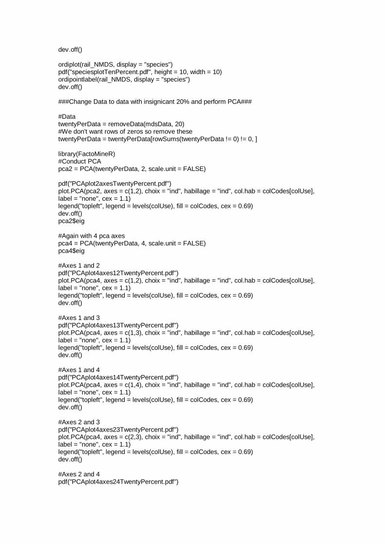
dev.off() ordiplot(rail_NMDS, display = "species") pdf("speciesplotTenPercent.pdf", height = 10, width = 10) ordipointlabel(rail_NMDS, display = "species") dev.off() ###Change Data to data with insignicant 20% and perform PCA### #Data twentyPerData = removeData(mdsData, 20) #We don't want rows of zeros so remove these twentyPerData = twentyPerData[rowSums(twentyPerData != 0) != 0, ] library(FactoMineR) #Conduct PCA pca2 = PCA(twentyPerData, 2, scale.unit = FALSE) pdf("PCAplot2axesTwentyPercent.pdf") plot.PCA(pca2, axes = c(1,2), choix = "ind", habillage = "ind", col.hab = colCodes[colUse], label = "none", cex = 1.1) legend("topleft", legend = levels(colUse), fill = colCodes, cex = 0.69) dev.off() pca2$eig #Again with 4 pca axes pca4 = PCA(twentyPerData, 4, scale.unit = FALSE) pca4$eig #Axes 1 and 2 pdf("PCAplot4axes12TwentyPercent.pdf") plot.PCA(pca4, axes = c(1,2), choix = "ind", habillage = "ind", col.hab = colCodes[colUse], label = "none", cex = 1.1) legend("topleft", legend = levels(colUse), fill = colCodes, cex = 0.69) dev.off() #Axes 1 and 3 pdf("PCAplot4axes13TwentyPercent.pdf") plot.PCA(pca4, axes = c(1,3), choix = "ind", habillage = "ind", col.hab = colCodes[colUse], label = "none", cex = 1.1) legend("topleft", legend = levels(colUse), fill = colCodes, cex = 0.69) dev.off() #Axes 1 and 4 pdf("PCAplot4axes14TwentyPercent.pdf") plot.PCA(pca4, axes = c(1,4), choix = "ind", habillage = "ind", col.hab = colCodes[colUse], label = "none", cex = 1.1) legend("topleft", legend = levels(colUse), fill = colCodes, cex = 0.69) dev.off() #Axes 2 and 3 pdf("PCAplot4axes23TwentyPercent.pdf") plot.PCA(pca4, axes = c(2,3), choix = "ind", habillage = "ind", col.hab = colCodes[colUse], label = "none", cex = 1.1) legend("topleft", legend = levels(colUse), fill = colCodes, cex = 0.69) dev.off() #Axes 2 and 4 pdf("PCAplot4axes24TwentyPercent.pdf")

plot.PCA(pca4, axes = c(2,4), choix = "ind", habillage = "ind", col.hab = colCodes[colUse], label = "none", cex = 1.1) legend("topright", legend = levels(colUse), fill = colCodes, cex = 0.69) dev.off() #Axes 3 and 4 pdf("PCAplot4axes34TwentyPercent.pdf") plot.PCA(pca4, axes = c(3,4), choix = "ind", habillage = "ind", col.hab = colCodes[colUse], label = "none", cex = 1.1) legend("topright", legend = levels(colUse), fill = colCodes, cex = 0.69) dev.off() ###NMDS of 20% data### library(vegan) #Perform NMDS rail_NMDS = metaMDS(comm = twentyPerData, k = 2, trymax = 100, autotransform = FALSE) #Sheperd Plot pdf("sheperdplotTwentyPercent.pdf") stressplot(rail_NMDS) dev.off() #Scatter plots pdf("sitesplotTwentyPercent.pdf") plot(rail_NMDS, display = "sites") orditorp(rail_NMDS, display = "sites", col = colCodes[colUse], pch = 19, labels = FALSE) legend("topleft", legend = levels(colUse), fill = colCodes, cex = 0.69) dev.off() ordiplot(rail_NMDS, display = "species") pdf("speciesplotTwentyPercent.pdf", height = 10, width = 10) ordipointlabel(rail_NMDS, display = "species") dev.off() ###Change Data to 30% and perform PCA### #Data thirtyPerData = removeData(mdsData, 30) thirtyPerData = thirtyPerData[rowSums(thirtyPerData != 0) != 0, ] library(FactoMineR) #Conduct PCA pca2 = PCA(thirtyPerData, 2, scale.unit = FALSE) pdf("PCAplot2axesThirtyPercent.pdf") plot.PCA(pca2, axes = c(1,2), choix = "ind", habillage = "ind", col.hab = colCodes[colUse], label = "none", cex = 1.1) legend("topleft", legend = levels(colUse), fill = colCodes, cex = 0.69) dev.off() pca2$eig #Again with 4 pca axes pca4 = PCA(thirtyPerData, 4, scale.unit = FALSE) pca4$eig #Axes 1 and 2 pdf("PCAplot4axes12ThirtyPercent.pdf")

plot.PCA(pca4, axes = c(1,2), choix = "ind", habillage = "ind", col.hab = colCodes[colUse], label = "none", cex = 1.1) legend("topleft", legend = levels(colUse), fill = colCodes, cex = 0.69) dev.off() #Axes 1 and 3 pdf("PCAplot4axes13ThirtyPercent.pdf") plot.PCA(pca4, axes = c(1,3), choix = "ind", habillage = "ind", col.hab = colCodes[colUse], label = "none", cex = 1.1) legend("topleft", legend = levels(colUse), fill = colCodes, cex = 0.69) dev.off() #Axes 1 and 4 pdf("PCAplot4axes14ThirtyPercent.pdf") plot.PCA(pca4, axes = c(1,4), choix = "ind", habillage = "ind", col.hab = colCodes[colUse], label = "none", cex = 1.1) legend("topleft", legend = levels(colUse), fill = colCodes, cex = 0.69) dev.off() #Axes 2 and 3 pdf("PCAplot4axes23ThirtyPercent.pdf") plot.PCA(pca4, axes = c(2,3), choix = "ind", habillage = "ind", col.hab = colCodes[colUse], label = "none", cex = 1.1) legend("topleft", legend = levels(colUse), fill = colCodes, cex = 0.69) dev.off() #Axes 2 and 4 pdf("PCAplot4axes24ThirtyPercent.pdf") plot.PCA(pca4, axes = c(2,4), choix = "ind", habillage = "ind", col.hab = colCodes[colUse], label = "none", cex = 1.1) legend("topright", legend = levels(colUse), fill = colCodes, cex = 0.69) dev.off() #Axes 3 and 4 pdf("PCAplot4axes34ThirtyPercent.pdf") plot.PCA(pca4, axes = c(3,4), choix = "ind", habillage = "ind", col.hab = colCodes[colUse], label = "none", cex = 1.1) legend("topright", legend = levels(colUse), fill = colCodes, cex = 0.69) dev.off() ###NMDS of 30% data### library(vegan) #Perform NMDS rail_NMDS = metaMDS(comm = thirtyPerData, k = 2, trymax = 100, autotransform = FALSE) #Sheperd Plot pdf("sheperdplotThirtyPercent.pdf") stressplot(rail_NMDS) #dev.off() #Scatter plots pdf("sitesplotThirtyPercent.pdf") plot(rail_NMDS, display = "sites") orditorp(rail_NMDS, display = "sites", col = colCodes[colUse], pch = 19, labels = FALSE) legend("topleft", legend = levels(colUse), fill = colCodes, cex = 0.69) dev.off() ordiplot(rail_NMDS, display = "species")

pdf("speciesplotThirtyPercent.pdf", width = 9) ordipointlabel(rail_NMDS, display = "species") dev.off() #Rail Data for Ellenberg F and N plotting #Robert Ashton #01/06/14 setwd("C:\\RFiles\\RailTrack\\Ellenberg\\") ellenbergData = read.csv(file = "EllenbergImport.csv", stringsAsFactors = FALSE, header = TRUE, sep = ",") names(ellenbergData) str(ellenbergData) abandonedTime = ellenbergData[247, c(-2,-1)] ellenbergData = ellenbergData[-247, ] ellenbergF = ellenbergData[ , 1] ellenbergN = ellenbergData[ , 2] ellenbergData = ellenbergData[ , 3:176 ] #Fix abandoned since row abandonedNo = c() index = 1 for (x in abandonedTime){ abandonedNo[index] = as.numeric(x) index = index +1 } #Ellenberg N mean notZero = c() index2 = 1 index3 = 1 ellenbergNAverage = c() for (column in ellenbergData){ for (value in column) { notZero[index2] = (value != 0) index2 = index2 + 1 } ellenbergNAverage[index3] = mean(ellenbergN[notZero], na.rm = TRUE) index2 = 1 index3 = index3 + 1 notZero = c() } pdf("EllenbergNMeanFix.pdf") plot(abandonedNo, ellenbergNAverage, xlab = "Time since abandonment (years)", ylab = "Mean (unweighted) Ellenberg N value per releve") dev.off() #EllenbergN Weighted Mean #29/07/14 notZero = c() index2 = 1 index3 = 1 ellenbergNWeightAverage = c() for (column in ellenbergData){ for (value in column) { notZero[index2] = (value != 0) index2 = index2 + 1

} ellenbergNWeightAverage[index3] = weighted.mean(ellenbergN[notZero], column[notZero], na.rm = TRUE) index2 = 1 index3 = index3 + 1 notZero = c() } pdf("EllenbergNWeightMean.pdf") plot(abandonedNo, ellenbergNWeightAverage) dev.off() #Ellenberg F mean notZero = c() index2 = 1 index3 = 1 ellenbergFAverage = c() for (column in ellenbergData){ for (value in column) { notZero[index2] = (value != 0) index2 = index2 + 1 } ellenbergFAverage[index3] = mean(ellenbergF[notZero], na.rm = TRUE) index2 = 1 index3 = index3 + 1 notZero = c() } pdf("EllenbergFMeanFix.pdf") plot(abandonedNo, ellenbergFAverage, xlab = "Time since abandonment (years)", ylab = "Mean (unweighted) Ellenberg F value per releve") dev.off() #EllenbergF Weighted Mean notZero = c() index2 = 1 index3 = 1 ellenbergFWeightAverage = c() for (column in ellenbergData){ for (value in column) { notZero[index2] = (value != 0) index2 = index2 + 1 } ellenbergFWeightAverage[index3] = weighted.mean(ellenbergF[notZero], column[notZero], na.rm = TRUE) index2 = 1 index3 = index3 + 1 notZero = c() } pdf("EllenbergFWeigthMean.pdf") plot(abandonedNo, ellenbergFWeightAverage) dev.off() #Ellenberg N Mean of Means #Separate mean values by site groups = c(rep("AM", 5), rep("APC", 4), rep("APE", 4), rep("APW", 3), rep("BFC", 6), rep("BFE", 5), rep("BFO", 3), rep("CN", 5), rep("CA", 10), rep("FN", 5), rep("FS", 5), rep("G-O", 5), rep("GA", 3), rep("GN", 5), rep("GSI", 6), rep("GS", 5), rep("H-ST.IE", 3), rep("H-
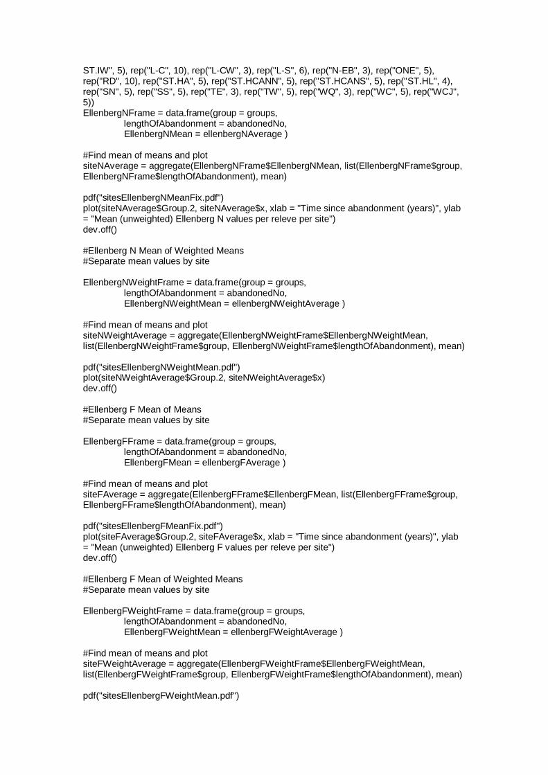
ST.IW", 5), rep("L-C", 10), rep("L-CW", 3), rep("L-S", 6), rep("N-EB", 3), rep("ONE", 5), rep("RD", 10), rep("ST.HA", 5), rep("ST.HCANN", 5), rep("ST.HCANS", 5), rep("ST.HL", 4), rep("SN", 5), rep("SS", 5), rep("TE", 3), rep("TW", 5), rep("WQ", 3), rep("WC", 5), rep("WCJ", 5)) EllenbergNFrame = data.frame(group = groups, lengthOfAbandonment = abandonedNo, EllenbergNMean = ellenbergNAverage ) #Find mean of means and plot siteNAverage = aggregate(EllenbergNFrame$EllenbergNMean, list(EllenbergNFrame$group, EllenbergNFrame$lengthOfAbandonment), mean) pdf("sitesEllenbergNMeanFix.pdf") plot(siteNAverage$Group.2, siteNAverage$x, xlab = "Time since abandonment (years)", ylab = "Mean (unweighted) Ellenberg N values per releve per site") dev.off() #Ellenberg N Mean of Weighted Means #Separate mean values by site EllenbergNWeightFrame = data.frame(group = groups, lengthOfAbandonment = abandonedNo, EllenbergNWeightMean = ellenbergNWeightAverage ) #Find mean of means and plot siteNWeightAverage = aggregate(EllenbergNWeightFrame$EllenbergNWeightMean, list(EllenbergNWeightFrame$group, EllenbergNWeightFrame$lengthOfAbandonment), mean) pdf("sitesEllenbergNWeightMean.pdf") plot(siteNWeightAverage$Group.2, siteNWeightAverage$x) dev.off() #Ellenberg F Mean of Means #Separate mean values by site EllenbergFFrame = data.frame(group = groups, lengthOfAbandonment = abandonedNo, EllenbergFMean = ellenbergFAverage ) #Find mean of means and plot siteFAverage = aggregate(EllenbergFFrame$EllenbergFMean, list(EllenbergFFrame$group, EllenbergFFrame$lengthOfAbandonment), mean) pdf("sitesEllenbergFMeanFix.pdf") plot(siteFAverage$Group.2, siteFAverage$x, xlab = "Time since abandonment (years)", ylab = "Mean (unweighted) Ellenberg F values per releve per site") dev.off() #Ellenberg F Mean of Weighted Means #Separate mean values by site EllenbergFWeightFrame = data.frame(group = groups, lengthOfAbandonment = abandonedNo, EllenbergFWeightMean = ellenbergFWeightAverage ) #Find mean of means and plot siteFWeightAverage = aggregate(EllenbergFWeightFrame$EllenbergFWeightMean, list(EllenbergFWeightFrame$group, EllenbergFWeightFrame$lengthOfAbandonment), mean) pdf("sitesEllenbergFWeightMean.pdf")

plot(siteFWeightAverage$Group.2, siteFWeightAverage$x) dev.off() #Cluster analysis of vegetative data from railways #07/07/14 #Robert Ashton setwd("C:\\RFiles\\RailTrack\\Cluster\\") railData = read.csv(file = "ImportData.csv", stringsAsFactors = FALSE, header = TRUE, sep = ",", row.names = 1) names(railData) str(railData) #Convert to matrix for use in metaMDS mdsData = data.matrix(railData) str(mdsData) names(mdsData) colUse = as.factor(gsub("\\d", "", row.names(railData))) colCodes = c("#000000", "#FFFF00", "#1CE6FF", "#FF34FF", "#FF4A46", "#008941", "#006FA6", "#A30059", "#FFDBE5", "#7A4900", "#0000A6", "#63FFAC", "#B79762", "#004D43", "#8FB0FF", "#997D87", "#5A0007", "#809693", "#FF0800", "#1B4400", "#4FC601", "#3B5DFF", "#4A3B53", "#FF2F80", "#61615A", "#BA0900", "#6B7900", "#00C2A0", "#FFAA92", "#FF90C9", "#B903AA", "#D16100", "#DDEFFF", "#000035", "#7B4F4B") colCodes2 = rainbow(35) colVec = colCodes[colUse] ###06/04/14### ###Heierachical Cluser Analysis### library(labdsv) library(ape) distData = dsvdis(mdsData, "steinhaus") clustAnal = hclust(distData, "ward.D", members = NULL) clustPhy = as.phylo(clustAnal) pdf("clusterPlotNew.pdf", width = 20, height = 7) par(mar = c(0,0,3,0)) plot(clustPhy, cex = 0.5, tip.color = colVec, direction = "downwards", main = "Hierachical Clustering using Steinhaus Coeff and Ward Clustering Method 07/04/14") dev.off() clustAnalD = as.dendrogram(clustAnal) clusMember = cutree(clustAnal, 35) colLab <- function(n) { if (is.leaf(n)) { a <- attributes(n) labCol <- colCodes[clusMember[which(names(clusMember) == a$label)]] attr(n, "nodePar") <- c(a$nodePar, lab.col = labCol, cexlab = 0.5, pch = NA) } n }

clusDendro = dendrapply(clustAnalD, colLab) plot(clusDendro, leaflab = 0.5) ###15/08/14### #Indicator Species Analyis #Remove empty species mdsDataRM = mdsData[ , -which(colnames(mdsData) %in% c("Bryum.caespiticium"))] cut2 = cutree(clustAnal, k = 2) indValue2 = indval(mdsDataRM, cut2) cut7 = cutree(clustAnal, k = 7) indValue7 = indval(mdsDataRM, cut7) ###TRY INDICSPECIES PACKAGE### library(indicspecies) cut7 = cutree(clustAnal, k = 7) indValueMulti7 = multipatt(data.frame(mdsDataRM), cut7, control = how(nperm=999)) indValueMulti2 = multipatt(data.frame(mdsDataRM), cut2, control = how(nperm = 999)) cut4 = cutree(clustAnal, k = 4) indValue4 = indval(mdsDataRM, cut4) ###16/08/14### dendro = as.dendrogram(clustAnal) plot(dendro) plot(cut(dendro, h = 2.75)$upper, main = "Upper tree of cut at h=2.75") par(cex = 1, mar = c(5,8,4,1)) plotting = plot(cut(dendro, h = 4)$upper, main = "", leaflab = "textlike") labels(plotting, label = c("a","b")) par(cex = 1) title(main = "Hierachical Clustering Using Steinhaus Coeff and Ward Clustering Method 07/04/14") axis(2) ###Try new approach with dendextend package### library(dendextend) dendro = as.dendrogram(clustAnal) top2Clusts = cut(dendro, h = 4)$upper y = data.frame(c("Senecio.jacobaea", 0.686, 0.001, "***"), c("Dactylis.glomerata", 0.591, 0.002, "**"), c("Vulpia.bromoides", 0.534, 0.001, "***")) spec1 = c("Senecio.jacobaea", "Dactylis.glomerata", "Vulpia.bromoides") stat1 = c(0.686, 0.591, 0.534) pVal1 = c(0.001, 0.002, 0.001) star1 = c("***", "**", "***")

clust1DF = data.frame(spec1, stat1, pVal1, star1) labels(top2Clusts) = list(clust1DF, "Cluster 2") labels_colors(top2Clusts) = c(2, 3) par(mar = c(5,8,4,1)) plot(top2Clusts, leaflab = "t", main = "Hierachical Clustering Using Steinhaus Coeff and Ward Clustering Method With Two Clusters 07/04/14") #####Simplified version##### ##Practice## library(dendextend) dendro = as.dendrogram(clustAnal) top2Clusts = cut(dendro, h = 4)$upper top2Clusts = hang.dendrogram(top2Clusts, hang = -1) labels(top2Clusts) = c("A", "B") plot(top2Clusts, axes = FALSE, edgePar = list(p.lty = 0, p.lwd = 20)) ##PLOT FOR 7 CLUSTERS## top7Clusts = cut(dendro, h = 2.75)$upper top7Clusts = hang.dendrogram(top7Clusts, hang = -1) labels(top7Clusts) = c("A - 19", "B - 14", "C - 40", "D - 10", "E - 14", "F - 11", "G- 66") pdf("clusterPlot7Clusters.pdf", width = 10) plot(top7Clusts, axes = FALSE, center = TRUE) dev.off() ### 18/09/14 ### ##Code to take 7 clusters and calculate mean time and st dev ##for the clusters and see if there is a sig difference ##using ANOVA for unequal sample sizes abandonTime = read.csv(file = "yearabandonmentImport.csv", header = FALSE, sep = ",") abandonTime = as.numeric(abandonTime) clustAband = data.frame(cut7, abandonTime) meanAbandonByClust = tapply(clustAband$abandonTime, clustAband$cut7, FUN = mean) sdAbandonByClust = tapply(clustAband$abandonTime, clustAband$cut7, FUN = sd) write.csv(meanAbandonByClust, file = "MeanTimeSinceAbandonmentByCluster.csv") write.csv(sdAbandonByClust, file = "SDTimeSinceAbandonmentByCluster.csv") fm1 = aov(abandonTime~cut7, data = clustAband) anovaOfAbandonByClust = anova(fm1) ###04/10//14### ##Code to calculate fidelity, exclusivity, mean cover % within ##clusters and mean % cover outside of clusters. #Identify species which need to be plotted indValData = read.csv(file = "indValueImport.csv", stringsAsFactors = FALSE, header = TRUE, sep = ",", row.names = 1) names(indValData)

str(indValData) allIndicatorSpecies = rownames(indValData) reducedDF = data.frame(mdsData[, allIndicatorSpecies]) #Need to add a column for the clusters the sites belong to reducedDFCluster = data.frame(cut7, reducedDF) #Use code from previous calculations of presence for calculating #fidelity and exclusivity relevesPresentIn = function(columnVector) { totalRelevesPresentIn = 0 for (value in columnVector) { if (value != 0) { totalRelevesPresentIn = totalRelevesPresentIn + 1 } } return(totalRelevesPresentIn) } setToNA = function(columnVector) { columnVector[columnVector[] == 0 ] = NA return(columnVector) } fid.ex.Appearance = aggregate(reducedDFCluster, by = list(cut7), FUN = relevesPresentIn) fid.ex.Tot = aggregate(reducedDFCluster, by = list(cut7), FUN = sum) te = as.factor(indValData[,1]) levels(te) = c(3,5,4,6,7,2,1) indValData[ , 1] = te indValData[ ,2] = as.numeric(indValData[,2]) #Create list of names belonging to each cluster specIn1 = rownames(indValData)[indValData[ ,1] == 1] specIn2 = rownames(indValData)[indValData[ ,1] == 2] specIn3 = rownames(indValData)[indValData[ ,1] == 3] specIn4 = rownames(indValData)[indValData[ ,1] == 4] specIn5 = rownames(indValData)[indValData[ ,1] == 5] specIn6 = rownames(indValData)[indValData[ ,1] == 6] specIn7 = rownames(indValData)[indValData[ ,1] == 7] clust1App = fid.ex.Appearance[specIn1] clust1Tot = fid.ex.Tot[specIn1] clust2App = fid.ex.Appearance[specIn2] clust2Tot = fid.ex.Tot[specIn2] clust3App = fid.ex.Appearance[specIn3] clust3Tot = fid.ex.Tot[specIn3] clust4App = fid.ex.Appearance[specIn4] clust4Tot = fid.ex.Tot[specIn4] clust5App = fid.ex.Appearance[specIn5] clust5Tot = fid.ex.Tot[specIn5] clust6App = fid.ex.Appearance[specIn6] clust6Tot = fid.ex.Tot[specIn6] clust7App = fid.ex.Appearance[specIn7] clust7Tot = fid.ex.Tot[specIn7]
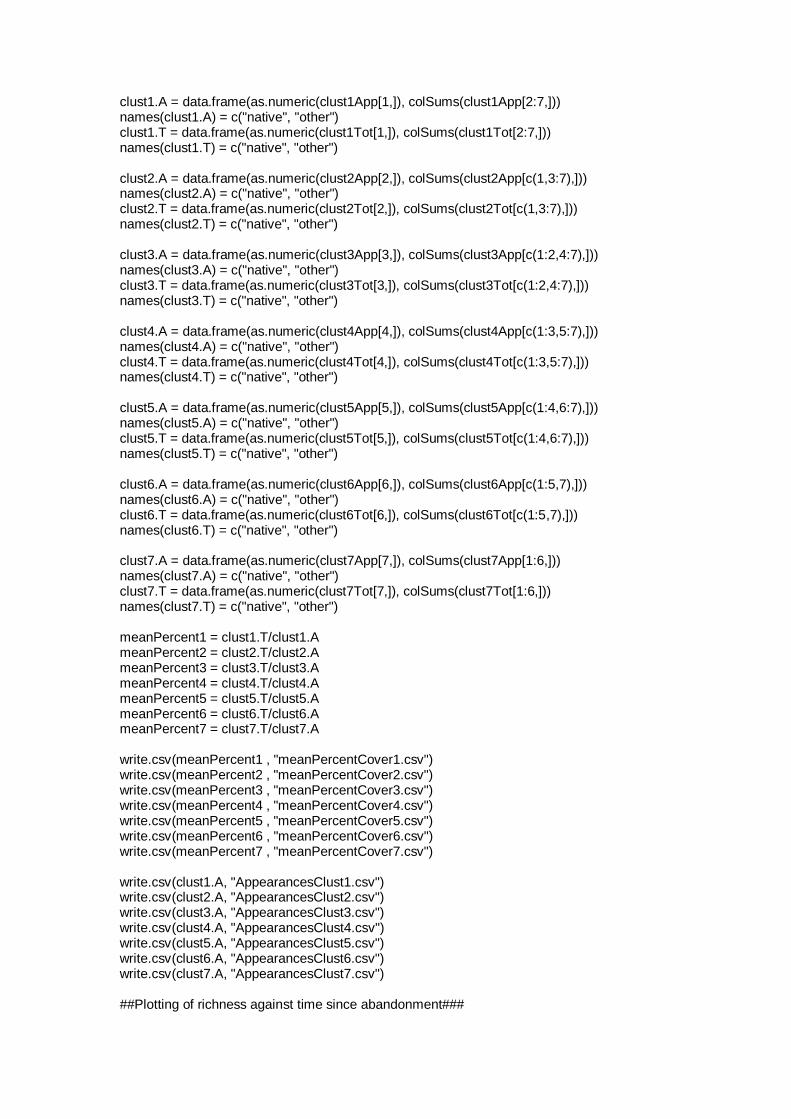
clust1.A = data.frame(as.numeric(clust1App[1,]), colSums(clust1App[2:7,])) names(clust1.A) = c("native", "other") clust1.T = data.frame(as.numeric(clust1Tot[1,]), colSums(clust1Tot[2:7,])) names(clust1.T) = c("native", "other") clust2.A = data.frame(as.numeric(clust2App[2,]), colSums(clust2App[c(1,3:7),])) names(clust2.A) = c("native", "other") clust2.T = data.frame(as.numeric(clust2Tot[2,]), colSums(clust2Tot[c(1,3:7),])) names(clust2.T) = c("native", "other") clust3.A = data.frame(as.numeric(clust3App[3,]), colSums(clust3App[c(1:2,4:7),])) names(clust3.A) = c("native", "other") clust3.T = data.frame(as.numeric(clust3Tot[3,]), colSums(clust3Tot[c(1:2,4:7),])) names(clust3.T) = c("native", "other") clust4.A = data.frame(as.numeric(clust4App[4,]), colSums(clust4App[c(1:3,5:7),])) names(clust4.A) = c("native", "other") clust4.T = data.frame(as.numeric(clust4Tot[4,]), colSums(clust4Tot[c(1:3,5:7),])) names(clust4.T) = c("native", "other") clust5.A = data.frame(as.numeric(clust5App[5,]), colSums(clust5App[c(1:4,6:7),])) names(clust5.A) = c("native", "other") clust5.T = data.frame(as.numeric(clust5Tot[5,]), colSums(clust5Tot[c(1:4,6:7),])) names(clust5.T) = c("native", "other") clust6.A = data.frame(as.numeric(clust6App[6,]), colSums(clust6App[c(1:5,7),])) names(clust6.A) = c("native", "other") clust6.T = data.frame(as.numeric(clust6Tot[6,]), colSums(clust6Tot[c(1:5,7),])) names(clust6.T) = c("native", "other") clust7.A = data.frame(as.numeric(clust7App[7,]), colSums(clust7App[1:6,])) names(clust7.A) = c("native", "other") clust7.T = data.frame(as.numeric(clust7Tot[7,]), colSums(clust7Tot[1:6,])) names(clust7.T) = c("native", "other") meanPercent1 = clust1.T/clust1.A meanPercent2 = clust2.T/clust2.A meanPercent3 = clust3.T/clust3.A meanPercent4 = clust4.T/clust4.A meanPercent5 = clust5.T/clust5.A meanPercent6 = clust6.T/clust6.A meanPercent7 = clust7.T/clust7.A write.csv(meanPercent1 , "meanPercentCover1.csv") write.csv(meanPercent2 , "meanPercentCover2.csv") write.csv(meanPercent3 , "meanPercentCover3.csv") write.csv(meanPercent4 , "meanPercentCover4.csv") write.csv(meanPercent5 , "meanPercentCover5.csv") write.csv(meanPercent6 , "meanPercentCover6.csv") write.csv(meanPercent7 , "meanPercentCover7.csv") write.csv(clust1.A, "AppearancesClust1.csv") write.csv(clust2.A, "AppearancesClust2.csv") write.csv(clust3.A, "AppearancesClust3.csv") write.csv(clust4.A, "AppearancesClust4.csv") write.csv(clust5.A, "AppearancesClust5.csv") write.csv(clust6.A, "AppearancesClust6.csv") write.csv(clust7.A, "AppearancesClust7.csv") ##Plotting of richness against time since abandonment###
##18/08/14## #Robert Ashton# setwd("C:\\RFiles\\RailTrack\\Richnes & Diversity\\") railData = read.csv(file = "ImportData.csv", stringsAsFactors = FALSE, header = TRUE, sep = ",", row.names = 1) names(railData) str(railData) #Convert to matrix for easy use dataMatrix = data.matrix(railData) str(dataMatrix) names(dataMatrix) #Import year since abandondment data sinceAbandon = read.csv(file = "yearAbandonmentImport.csv", header = FALSE) sinceAbandon = as.numeric(sinceAbandon) totalNonZero = function(Row){ nonZero = 0 for (value in Row){ if (value == 0){ } else { nonZero = nonZero + 1 } } return(nonZero) } richness = apply(dataMatrix, MARGIN = 1, FUN = totalNonZero) pdf("abandonedTimeVRichness.pdf") plot(sinceAbandon, richness) dev.off() groups = c(rep("AM", 5), rep("APC", 4), rep("APE", 4), rep("APW", 3), rep("BFC", 6), rep("BFE", 5), rep("BFO", 3), rep("CN", 5), rep("CA", 10), rep("FN", 5), rep("FS", 5), rep("G-O", 5), rep("GA", 3), rep("GN", 5), rep("GSI", 6), rep("GS", 5), rep("H-ST.IE", 3), rep("H-ST.IW", 5), rep("L-C", 10), rep("L-CW", 3), rep("L-S", 6), rep("N-EB", 3), rep("ONE", 5), rep("RD", 10), rep("ST.HA", 5), rep("ST.HCANN", 5), rep("ST.HCANS", 5), rep("ST.HL", 4), rep("SN", 5), rep("SS", 5), rep("TE", 3), rep("TW", 5), rep("WQ", 3), rep("WC", 5), rep("WCJ", 5)) RichnessFrame = data.frame(group = groups, lengthOfAbandonment = sinceAbandon, rich = richness ) siteRichnessMean = aggregate(RichnessFrame$rich, list(RichnessFrame$group, RichnessFrame$lengthOfAbandonment), mean) pdf("abandonedTimeVRichnessMEANOFSITESfix.pdf") plot(siteRichnessMean$Group.2, siteRichnessMean$x, xlab = "Time since abandonment (years)", ylab = "Mean richness per site") dev.off() ##Diversity## library(vegan)
divData = diversity(dataMatrix, index = "shannon", MARGIN = 1, base = exp(1)) pdf("abandonedTimeVDiversity.pdf") plot(sinceAbandon, divData) dev.off() diversityFrame = data.frame(group = groups, lengthOfAbandonment = sinceAbandon, div = divData ) siteDiversityMean = aggregate(diversityFrame$div, list(diversityFrame$group, diversityFrame$lengthOfAbandonment), mean) pdf("abandonedTimeVDiversityMEANOFSITESfix.pdf") plot(siteDiversityMean$Group.2, siteDiversityMean$x, xlab = "Time since abandonment (years)", ylab = "Mean diversity per site") dev.off() ### 18/09/14 ### ## Robert Ashton # ## Code to find how abundent a species is and then write ## this to a csv file, also write to csv all species which ## are only present in one releve. Also writes as a csv all ## species which are present in 20 or more releves. setwd("C:\\RFiles\\RailTrack\\Presence\\") railData = read.csv(file = "presenceData.csv", stringsAsFactors = FALSE, header = TRUE, sep = ",", row.names = 1) names(railData) str(railData) #Convert to matrix for use in metaMDS mdsData = data.matrix(railData) str(mdsData) names(mdsData) ##function to calculate how many releves present in relevesPresentIn = function(columnVector) { totalRelevesPresentIn = 0 for (value in columnVector) { if (value != 0) { totalRelevesPresentIn = totalRelevesPresentIn + 1 } } return(totalRelevesPresentIn) } presenceFrame = apply(mdsData, 2, FUN = relevesPresentIn) write.csv(presenceFrame, file = "presenceFrame.csv") removeAllButValueOne = function(aVector) { index = 1 removeVector = c() for (value in aVector) { if (value != 1) { removeVector = c(-index, removeVector)
} index = index + 1 } return(aVector[removeVector]) } onlyOne = removeAllButValueOne(presenceFrame) write.csv(onlyOne, file = "onlyOnePresent.csv") removeAllLessThan20 = function(aVector) { index = 1 removeVector = c() for (value in aVector) { if (value < 20) { removeVector = c(-index, removeVector) } index = index + 1 } return(aVector[removeVector]) } moreThan20 = removeAllLessThan20(presenceFrame) write.csv(moreThan20, file = "moreThan20Present.csv") ###04/10/14### ##We are also interested in the mean percent cover of ##each species in a releve. Write code to find this #Need to loop over each species like above but sum the values. #Easy mode setToNA = function(columnVector) { columnVector[columnVector[] == 0 ] = NA return(columnVector) } mdsNA = apply(mdsData, 2 , FUN = setToNA) means = apply(mdsNA, 2, FUN = mean, na.rm = TRUE) sds = apply(mdsNA, 2, FUN = sd, na.rm = TRUE) greater20DF = data.frame(moreThan20, round(means[names(moreThan20)]), round(sds[names(moreThan20)])) write.csv(greater20DF, "greater20Frame.csv") ###21/09/14### ##Robert Ashton## #Canonical Correspondence Analysis# setwd("C:\\RFiles\\RailTrack\\Environmental\\") railData = read.csv(file = "CCAImport.csv", stringsAsFactors = FALSE, header = TRUE, sep = ",", row.names = 1) names(railData) str(railData) #Convert to matrix for easy use

dataMatrix = data.matrix(railData) str(dataMatrix) names(dataMatrix) #Separate Matrices speciesMatrix = dataMatrix[ , 1:246] envMatrix = dataMatrix[ , 247:261] #Need to standardise the env matrix. ## 23/09/14 ## library(vegan) standEnv = decostand(envMatrix, method = "range", MARGIN = 2, na.rm = TRUE) # Perform CCA spe.cca1 = cca(speciesMatrix, standEnv[ , 1:5] , na.action = na.omit) pdf("CCA_with_Alt,Asp,Yr,Rain,SumTem.pdf") plot(spe.cca1, display = c("sites", "bp"), type = "text") dev.off() #remove NA rows noNAData = na.omit(dataMatrix) speciesNoNA = noNAData[ , 1:246] envMatrixNoNA = noNAData[ , 247:261] spe.cca2 = cca(speciesNoNA, envMatrixNoNA[ , 6:15], na.action = na.omit) pdf("CCA_with_pH,Mois,Org,Mg,Pb,K,Ca,Cu,Cd,Ni.pdf") plot(spe.cca2, display = c("sites", "bp"), type = "text") dev.off() spe.cca3 = cca(speciesNoNA, envMatrixNoNA, na.action = na.omit) pdf("CCA_with_All.pdf") plot(spe.cca3, display = c("sites", "bp"), type = "text") dev.off() # Test with just SummerTemp, Rainfall spe.cca4 = cca(speciesMatrix, standEnv[ ,4:5], na.action = na.omit) pdf("CCA_with_SumTemp,Rainfall.pdf") plot(spe.cca4, display = c("sites", "bp"), type = "text") dev.off() # Plot with SummerTemp, Rainfall and PH #find no NA for PH noPHNA = na.omit(dataMatrix[ , 1:252]) speciesNoPHNA = noPHNA[ ,1:246] envMatrixNoPHNA = noPHNA[ ,247:252] spe.cca5 = cca(speciesNoPHNA, envMatrixNoPHNA[,4:6], na.action = na.omit) pdf("CCA_with_SumTemp,Rainfall,pH.pdf") plot(spe.cca5, display = c("sites", "bp"), type = "text") dev.off() ###24/09/14### ##Plot with site scaling## plot(spe.cca1, scaling = 1, display = c("sites", "bp"), type = "text") # Same as above, suggests done by default

#Use cut from wards clustering method# library(labdsv) distData = dsvdis(speciesMatrix, "steinhaus") clustAnal = hclust(distData, "ward.D", members = NULL) cut7 = cutree(clustAnal, k = 7) #Identify species which need to be plotted indSpec1 = c("Festuca.rubra") indSpec2 = c("Schistidium.crassipilum", "Urtica.dioica", "Cardamine.flexuosa", "Schistidium.apocarpum", "Barbula.convoluta" ,"Epilobium.montanum") indSpec3 = c("Epilobium.ciliatum", "Geranium.robertianum", "Fraxinus.excelsior") indSpec4 = c("Arrhenatherum.elatius") indSpec5 = c("Eupatorium.cannabinum", "Agrostis.stolonifera") indSpec6 = c("Vulpia.bromoides", "Galium.aparine", "Anthriscus.sylvestris", "Pimpinella.saxifraga" ,"Veronica.arvensis", "Picris.echioides", "Sonchus.asper") indSpec7 = c("Linaria.vulgaris", "Deschampsia.cespitosa", "Tanacetum.vulgare", "Bryum.argenteum", "Betula.pendula", "Agrostis.capillaris") indSpec = c(indSpec1, indSpec2, indSpec3, indSpec4, indSpec5, indSpec6, indSpec7) indSpecLab1 = c("Fe.rub.") indSpecLab2 = c("Sc.cras.", "Ur.dio.", "Ca.flex.", "Sc.apoc.", "Ba.con.", "Ep.mont.") indSpecLab3 = c("Ep.cil.", "Ge.rob.", "Fr.exce.") indSpecLab4 = c("Ar.elat.") indSpecLab5 = c("Eu.can.", "Ag.stol.") indSpecLab6 = c("Vu.bro.", "Ga.apar.", "An.syl.", "Pi.sax.", "Ve.arv.", "Pi.ech.", "So.asp.") indSpecLab7 = c("Li.vul.", "De.ces.", "Ta.vul.", "Br.arg.", "Be.pen.", "Ag.cap.") indSpecLab = c(indSpecLab1, indSpecLab2, indSpecLab3, indSpecLab4, indSpecLab5, indSpecLab6, indSpecLab7) indSpecClust = c(1, rep(2, 6), rep(3, 3), 4, rep(5, 2), rep(6, 7), rep(7, 6)) #set colours for legened and points leg.text = c("A", "B", "C", "D", "E", "F", "G") leg.col = c("#49FF00FF", "#0092FFFF", "#FF8000FF", "#4900FFFF", "#222A0AFF", "#FFDB00FF", "#FF0000FF") colUse = c("#FF0000FF", "#FFDB00FF", "#49FF00FF", "#FF8000FF", "#0092FFFF", "#4900FFFF", "#222A0AFF")[cut7] #For Alt, Asp, Year, Rainfall, and Summer Temp pdf("CCA_Coloured_with_A,A,Y,R,S_ColFix.pdf") plot(spe.cca1, scaling = 1, type = "none", xlim = c(-5.5,5), ylim = c(-4,4)) points(spe.cca1, display = "sites", col = colUse) text(spe.cca1, display = "species", select = indSpec, labels = indSpecLab, col = rainbow(7)[indSpecClust], pch = 3) points(spe.cca1, display = "bp") text(spe.cca1, display = "bp") legend("topleft", legend = leg.text, fill = leg.col) dev.off() #For pH, moisture, organic content, Mg, Pb, K, Ca, Cu, Cd, Ni pdf("CCA_Coloured_with_ph,M,O,Mg,Pb,K,Ca,Cu,Cd,Ni_ColFix.pdf") plot(spe.cca2, scaling = 1, type = "none", xlim = c(-3, 2), ylim = c(-2, 2)) points(spe.cca2, display = "sites", col = colUse) points(spe.cca2, display = "species", select = indSpec, col = rainbow(7)[indSpecClust], pch = 3) points(spe.cca2, display = "bp")

text(spe.cca2, display = "bp") legend("bottomleft", legend = leg.text, fill = leg.col) dev.off() #For all environmental variables pdf("CCA_Coloured_with_all_ColFix.pdf") plot(spe.cca3, scaling = 1, type = "none", xlim = c(-4.5, 4), ylim = c(-1.5, 4)) points(spe.cca3, display = "sites", col = colUse) points(spe.cca3, display = "species", select = indSpec, col = rainbow(7)[indSpecClust], pch = 3) points(spe.cca3, display = "bp") text(spe.cca3, display = "bp") legend("topright", legend = leg.text, fill = leg.col) dev.off() ###03/10/14### ##We want to label the corsses in the above diagrams instead ##with the species names. To do this we convert to a data frame ##and use the setnames function in the data.table package and ##then convert back to a matrix and complete the plotting again. library(data.table) tempDF = data.frame(dataMatrix) setnames(tempDF, indSpec, indSpecLab) dataMatrixLab = data.matrix(tempDF) speciesMatrixLab = dataMatrixLab[ , 1:246] envMatrixLab = dataMatrixLab[ , 247:261] standEnvLab = decostand(envMatrixLab, method = "range", MARGIN = 2, na.rm = TRUE) spe.cca1Lab = cca(speciesMatrixLab, standEnvLab[ , 1:5] , na.action = na.omit) noNADataLab = na.omit(dataMatrixLab) speciesNoNALab = noNADataLab[ , 1:246] envMatrixNoNALab = noNADataLab[ , 247:261] spe.cca2Lab = cca(speciesNoNALab, envMatrixNoNALab[ , 6:15], na.action = na.omit) spe.cca3Lab = cca(speciesNoNALab, envMatrixNoNALab, na.action = na.omit) #For Alt, Asp, Year, Rainfall, and Summer Temp pdf("CCA_Coloured_with_A,A,Y,R,S_ColFix.pdf") plot(spe.cca1Lab, scaling = 1, type = "none", xlim = c(-5.5,5), ylim = c(-4,4)) points(spe.cca1Lab, display = "sites", col = colUse) text(spe.cca1Lab, display = "species", select = indSpecLab, col = rainbow(7)[indSpecClust], pch = 3) points(spe.cca1Lab, display = "bp") text(spe.cca1Lab, display = "bp") legend("topleft", legend = leg.text, fill = leg.col) dev.off() #For pH, moisture, organic content, Mg, Pb, K, Ca, Cu, Cd, Ni pdf("CCA_Coloured_with_ph,M,O,Mg,Pb,K,Ca,Cu,Cd,Ni_ColFix.pdf") plot(spe.cca2Lab, scaling = 1, type = "none", xlim = c(-3, 2), ylim = c(-2, 2)) points(spe.cca2Lab, display = "sites", col = colUse) text(spe.cca2Lab, display = "species", select = indSpecLab, col = rainbow(7)[indSpecClust], pch = 3) points(spe.cca2Lab, display = "bp") text(spe.cca2Lab, display = "bp") legend("bottomleft", legend = leg.text, fill = leg.col) dev.off() #For all environmental variables pdf("CCA_Coloured_with_all_ColFix.pdf")

plot(spe.cca3Lab, scaling = 1, type = "none", xlim = c(-4.5, 4), ylim = c(-1.5, 4)) points(spe.cca3Lab, display = "sites", col = colUse) text(spe.cca3Lab, display = "species", select = indSpecLab, col = rainbow(7)[indSpecClust], pch = 3) points(spe.cca3Lab, display = "bp") text(spe.cca3Lab, display = "bp") legend("topright", legend = leg.text, fill = leg.col) dev.off() #Significance testing anova(spe.cca1, step = 1000) ###01/10/14### spe.cca1.1 = cca(speciesMatrix ~ Altitude + Aspect + YearSinceClose + Rainfall + SummerTemp, data = data.frame(standEnv), na.action = na.omit) anova(spe.cca1.1, by = "terms", perm = 1000) spe.cca2.2 = cca(speciesMatrix ~ pH + Moisture + Organic + Mg + Pb + K + Ca + Cu + Cd + Ni, data = data.frame(standEnv), na.action = na.omit) m1 = update(spe.cca2.2, subset = -spe.cca2.2$na.action) anova(m1, by = "terms", perm = 1000) spe.cca3.3 = cca(speciesMatrix ~ ., data = data.frame(standEnv), na.action = na.omit) m2 <- update(spe.cca3.3, subset = -spe.cca3.3$na.action) anova(m2, by = "terms", perm = 1000) ###01/10/14### ##Calculate mean and SD of environmental variables for each ##cluster envCluster = data.frame(as.factor(cut7), envMatrix) colnames(envCluster)[1] = "cut7" meanByClust = aggregate(envCluster[,-1], by = list(envCluster$cut7), FUN = mean, na.rm = TRUE) sdByClust = aggregate(envCluster[,-1], by = list(envCluster$cut7), FUN = sd, na.rm = TRUE) write.csv(meanByClust, file = "meanByCluster.csv") write.csv(sdByClust, file = "sdByCluster.csv") ##WWrong code left in for reference## #aov.out = aov(cut7 ~ Altitude+Aspect+YearSinceClose+Rainfall+SummerTemp+pH*+Moisture+Organic+Mg+Pb+K+Ca+Cu+Cd+Ni, data = envCluster, na.action = na.exclude) #posthoc = TukeyHSD(x = aov.out, "Altitude", conf.level = 0.95) #aov.out2 = aov(cut7 ~ as.factor(Altitude), data = envCluster) #posthoc2 = TukeyHSD(x = aov.out2, "cut7") ###02/10/14### #Try as written down aAlt = aov(envCluster$Altitude ~ envCluster$cut7) posthocAlt = TukeyHSD(x = aAlt, "envCluster$cut7") aAsp = aov(envCluster$Aspect ~ envCluster$cut7) posthocAsp = TukeyHSD(x = aAsp, "envCluster$cut7") aYr = aov(envCluster$YearSinceClose ~ envCluster$cut7) posthocYr = TukeyHSD(x = aYr, "envCluster$cut7") aRai = aov(envCluster$Rainfall ~ envCluster$cut7)

posthocRai = TukeyHSD(x = aRai, "envCluster$cut7") aTmp = aov(envCluster$SummerTemp ~ envCluster$cut7) posthocTmp = TukeyHSD(x = aTmp, "envCluster$cut7") apH = aov(envCluster$pH ~ envCluster$cut7) posthocpH = TukeyHSD(x = apH, "envCluster$cut7") aMoi = aov(envCluster$Moisture ~ envCluster$cut7) posthocMoi = TukeyHSD(x = aMoi, "envCluster$cut7") aOrg = aov(envCluster$Organic ~ envCluster$cut7) posthocOrg = TukeyHSD(x = aOrg, "envCluster$cut7") aMg = aov(envCluster$Mg ~ envCluster$cut7) posthocMg = TukeyHSD(x = aMg, "envCluster$cut7") aPb = aov(envCluster$Pb ~ envCluster$cut7) posthocPb = TukeyHSD(x = aPb, "envCluster$cut7") aK = aov(envCluster$K ~ envCluster$cut7) posthocK = TukeyHSD(x = aK, "envCluster$cut7") aCa = aov(envCluster$Ca ~ envCluster$cut7) posthocCa = TukeyHSD(x = aCa, "envCluster$cut7") aCu = aov(envCluster$Cu ~ envCluster$cut7) posthocCu = TukeyHSD(x = aCu, "envCluster$cut7") aCd = aov(envCluster$Cd ~ envCluster$cut7) posthocCd = TukeyHSD(x = aCd, "envCluster$cut7") aNi = aov(envCluster$Ni ~ envCluster$cut7) posthocNi = TukeyHSD(x = aNi, "envCluster$cut7") ##03/10/14## #Using agricole package for Tukeys library(agricolae) hsdAlt = HSD.test(y = aAlt, trt = "envCluster$cut7") hsdAsp = HSD.test(y = aAsp, trt = "envCluster$cut7") hsdYr = HSD.test(y = aYr, trt = "envCluster$cut7") hsdRai = HSD.test(y = aRai, trt = "envCluster$cut7") hsdTmp = HSD.test(y = aTmp, trt = "envCluster$cut7") hsdpH = HSD.test(y = apH, trt = "envCluster$cut7") hsdMoi = HSD.test(y = aMoi, trt = "envCluster$cut7") hsdOrg = HSD.test(y = aOrg, trt = "envCluster$cut7") hsdMg = HSD.test(y = aMg, trt = "envCluster$cut7") hsdPb = HSD.test(y = aPb, trt = "envCluster$cut7") hsdK = HSD.test(y = aK, trt = "envCluster$cut7") hsdCa = HSD.test(y = aCa, trt = "envCluster$cut7") hsdCu = HSD.test(y = aCu, trt = "envCluster$cut7") hsdCd = HSD.test(y = aCd, trt = "envCluster$cut7") hsdNi = HSD.test(y = aNi, trt = "envCluster$cut7")

APPENDIX 3 – MAVIS ANALYSIS
Location Twinspan Mavis Light Wetness pH Fertility C S R
Amwlch 1 1 0 6.3 5.6 5.9 5.2 2.85 2.39 2.64
Amwlch 2 2 1 6.4 5.4 5.5 4.7 2.79 2.86 2.55
Amwlch 3 3 2 6.6 5.4 5.7 4.9 2.93 2.6 2.6
Amwlch 4 4 3 6 5.2 5.6 4.9 2.89 2.68 2.43
Amwlch 5 5 4 5.9 5.2 5.7 4.8 2.84 2.68 2.76
Appleby Shaded 1 6 5 5.9 6 5.9 5.8 1.77 2.62 3.31
Appleby Shaded 2 7 6 6 5.9 6.2 6 2.17 2.17 3.42
Appleby Shaded 3 8 7 5.7 6.6 6.1 5.8 2 2.11 3.44
Appleby Shaded 4 9 8 6.1 6.4 5.9 5.8 2.36 2.14 3.21
Appleby 1 10 9 6.6 5.3 6.2 5.9 2.82 2.45 2.64
Appleby 2 11 10 7.1 5.3 5.9 5.2 2.77 2.46 2.92
Appleby 3 12 11 6.7 5.2 5.8 5.5 2.61 2.21 3.18
Appleby 4 13 12 7 5.4 6.1 5.7 2.37 2.42 3.11
Appleby Wet 1 14 13 6.4 7.4 6.1 5.8 2.47 1.76 3.18
Appleby Wet 2 15 14 6.3 6.6 6.2 6.2 2.5 1.75 3.31
Appleby Wet 3 16 15 6.6 6 6.1 5.7 2.09 2.09 3.32
Bleanau Ffest Cutt. 1 17 16 6.4 5.3 5.9 5.2 3.32 2.56 2.04
Bleanau Ffest Cutt. 2 18 17 6.6 5.3 6.1 5.2 3.41 2.26 2.22
Bleanau Ffest Cutt. 3 19 18 6.5 5.3 6 5.2 3.62 2.14 1.9
Bleanau Ffest Cutt. 4 20 19 6.1 5.4 6.2 5.3 3.56 2.13 1.69
Bleanau Ffest Cutt. 5 21 20 5.3 5.8 6.8 6 4.5 1.5 1.2
Bleanau Ffest Cutt. 6 22 21 6.9 6.3 5.2 4.6 3 2.08 2.75
Bleanau Ffest Embankment 1 23 22 7.1 5.7 5.6 5 3.42 2.58 2.08
Bleanau Ffest Embankment 2 24 23 6.8 4.9 5.3 4.6 2.56 3.19 2.19
Bleanau Ffest Embankment 3 25 24 6.9 5.3 5.8 5.2 2.85 2.85 2.23
Bleanau Ffest Embankment 4 26 25 6.7 5.1 5.2 4 2.5 3.23 2.05
Bleanau Ffest Embankment 5 27 26 6.8 5.8 5.9 5.3 3.15 2.54 2.38
Bleanau Ffest Open 1 28 27 6.5 6.2 5 4.2 3.32 2.45 1.95
Bleanau Ffest Open 2 29 28 6.7 6.3 4.9 4.1 3.29 2.42 2.04
Bleanau Ffest Open 3 30 29 6.6 6.4 5.2 4.3 3.3 2.52 2.04
Cambridge 1 31 30 7.3 4.8 6.4 5.1 2.75 2.15 2.77
Cambridge 2 32 31 7.3 4.8 6.1 5 2.92 2.22 2.73
Cambridge 3 33 32 7.3 4.7 6.5 5.4 3 2 2.87
Cambridge 4 34 33 7.3 4.9 6.4 5.4 3.12 2.07 2.73
Cambridge 5 35 34 7.3 5.1 6.3 5.1 3 2.14 2.82
Carrington 1 36 35 7.1 5.4 5.9 4.7 3.1 1.62 2.81
Carrington 2 37 36 7.2 6.2 5.3 4.5 3.33 2.13 2.53
Carrington 3 38 37 6.9 6.1 5.7 4.6 3.88 1.88 1.88
Carrington 4 39 38 6.5 5.8 5.6 4.9 3.25 2.5 2.04
Carrington 5 40 39 7.1 5.9 5.4 4.4 3.21 2.13 2.33
Carrington 6 41 40 7.3 5.9 6 5.3 3.44 2.06 2.28

Carrington 7 42 41 7 5.5 6.2 5.3 3.58 1.84 2.42
Carrington 8 43 42 6.6 5.8 6.2 5.8 3.88 1.41 2.06
Carrington 9 44 43 7.2 5.6 6 5.2 3.18 2.18 2.71
Carrington 10 45 44 7 5.9 6.4 5.8 3.95 1.8 2
Fleetwood North 1 46 45 7.2 4.8 6.6 4.8 2.53 2.26 2.91
Fleetwood North 2 47 46 7.3 5.2 6.4 4.6 2.87 2.71 2.42
Fleetwood North 3 48 47 7.2 5.3 6.6 4.7 2.83 2.48 2.48
Fleetwood North 4 49 48 6.7 5.4 6.2 4.6 2.59 2.86 2.52
Fleetwood North 5 50 49 7.1 5.4 6.3 4.7 2.68 2.64 2.5
Fleetwood South 1 51 50 7.2 5.2 6.8 5.7 3.25 2 2.58
Fleetwood South 2 52 51 6.4 5.3 6.8 6 3.56 2.13 2.13
Fleetwood South 3 53 52 6.5 5 6.6 6 3.6 2.1 2.2
Fleetwood South 4 54 53 6.8 5.1 6.4 5.9 3.19 2.38 2.56
Fleetwood South 5 55 54 6.1 5.4 6.7 6.3 3.33 2.53 2.13
Gobowen Oswestry 1 56 55 6.2 5.2 6 6 3.17 1.89 2.61
Gobowen Oswestry 2 57 56 6.4 5.1 6.3 6.1 3.05 1.95 2.58
Gobowen Oswestry 3 58 57 6.4 5 6.1 5.9 2.95 2 2.63
Gobowen Oswestry 4 59 58 6.5 5 6.1 5.7 2.96 2.09 2.74
Gobowen Oswestry 5 60 59 6.6 4.8 6.4 5.9 3.21 1.71 2.64
Golborne Ash 1 61 60 7 6.3 5.8 4.9 4.25 1.75 1.75
Golborne Ash 2 62 61 7 6 5.9 5 3.92 2.08 1.92
Golborne Ash 3 63 62 7.1 5.9 6.2 5.8 3.9 2.1 2.1
Golborne North 1 64 63 7 5.3 6.2 5.1 2.74 2.29 3.06
Golborne North 2 65 64 7.1 5.3 6 4.9 2.83 2.61 2.96
Golborne North 3 66 65 7.1 5.2 6 5.1 2.84 2.4 2.96
Golborne North 4 67 66 7 5.3 5.9 5.2 3.13 2.53 2.73
Golborne North 5 68 67 7.1 5.3 6 5.1 2.76 2.29 3.06
Golborne Sidings 1 69 68 7 5.1 6.2 5.6 2.67 1.83 3.33
Golborne Sidings 2 70 69 7.2 5 6.5 5.6 2.7 1.9 3.3
Golborne Sidings 3 71 70 7.2 5.1 6.6 6 3.53 2.16 2.47
Golborne Sidings 4 72 71 7 5.4 6.6 6.2 3.38 1.79 2.63
Golborne Sidings 5 73 72 7.1 5.4 6.3 5.6 3.38 2.28 2.63
Golborne Sidings 6 74 73 7.2 5 6.6 5.9 2.94 2 2.94
Golborne South 1 75 74 6.8 5.3 6.1 5.8 3.35 1.87 2.57
Golborne South 2 76 75 7 5.2 6.1 5.9 3.5 1.82 2.5
Golborne South 3 77 76 6.9 5.3 6.3 6 3.65 1.75 2.35
Golborne South 4 78 77 6.8 5.1 6.7 6.3 3.75 1.81 2.25
Golborne South 5 79 78 7 5.1 7 7.1 4 1.6 2
Histon St Ives East 1 80 79 6.8 5.1 6.7 5.9 2.09 2.07 3.5
Histon St Ives East 2 81 80 6.9 5.4 6.7 6.1 2.71 2.12 2.9
Histon St Ives East 3 82 81 7 4.7 6.7 5.6 3.05 2.16 2.67
Histon St Ives West 1 83 82 7.2 4.8 6.6 5.1 2.42 2.15 3.13
Histon St Ives West 2 84 83 6.9 4.6 6.5 4.7 2.3 2.29 3.23
Histon St Ives West 3 85 84 7.1 4.8 6.6 4.9 2.45 2.47 2.8
Histon St Ives West 4 86 85 7.1 4.5 6.7 4.4 2.58 2.17 3.08
Histon St Ives West 5 87 86 7.2 4.9 6.5 4.8 2.79 2.31 2.93
Leek Cauldon 1 88 87 6.7 5.5 5.8 5.2 3.14 2.71 2.2

Leek Cauldon 2 89 88 7.1 5.3 6.1 5.1 3.29 2.42 2.61
Leek Cauldon 3 90 89 6.8 5.3 6.4 6 3.32 2.12 2.56
Leek Cauldon 4 91 90 6.9 5.6 6.1 5.7 3.58 2.32 2.26
Leek Cauldon 5 92 91 7 5.5 6.2 5.5 3.39 2.17 2.44
Leek Cauldon 6 93 92 6.7 5.3 6.1 5.1 3.1 2.3 2.78
Leek Cauldon 7 94 93 6.8 5.5 5.9 5.1 3.38 2 2.26
Leek Cauldon 8 95 94 6.7 5.6 5.9 5.2 3.38 2.44 2.44
Leek Cauldon 9 96 95 6.6 5.5 6.1 5.4 2.91 2.65 2.63
Leek Cauldon 10 97 96 7 5 6.3 5.6 3.2 2.27 2.8
Leek Cauldon West 1 98 97 6.7 5.5 6.4 5.5 3.44 1.84 2.56
Leek Cauldon West 2 99 98 5.8 6.1 5.5 5.2 3.3 2.5 2.03
Leek Cauldon West 3 100 99 6.5 5.3 5.9 5.3 2.83 1.96 2.91
Leek Stoke 1 101 100 7.1 5.2 6.2 5.1 2.74 1.91 3.11
Leek Stoke 2 102 101 6.8 5.3 6.3 5.4 2.68 2.1 2.77
Leek Stoke 3 103 102 6.9 5.3 6.1 4.6 3.06 2.31 2.61
Leek Stoke 4 104 103 7 5.7 5.7 4.6 2.94 2.48 2.56
Leek Stoke 5 105 104 7.1 5.4 6.1 5.1 3.02 2.21 3.74
Leek Stoke 6 106 105 7 5.7 5.9 5 3.24 2.36 2.4
Newport Ebbw Vale 1 107 106 6.7 5.4 6.6 5.8 2.84 2.03 2.86
Newport Ebbw Vale 2 108 107 6.9 5.4 6.6 5.7 3.19 1.98 2.72
Newport Ebbw vale 3 109 108 5.7 5.3 6.5 5.9 3.4 2.15 1.95
Oswestry N Embankment 1 110 109 7 5.1 6.1 5 2.41 2.49 2.89
Oswestry N Embankment 2 111 110 6.7 5.1 6.6 5.7 3.11 2.18 2.46
Oswestry N Embankment 3 112 111 6.8 5 6.9 5.9 3.29 2.29 2.29
Oswestry N Embankment 4 113 112 6.9 5.4 6.6 5.8 3.44 2.56 2.11
Oswestry N Embankment 5 114 113 7.2 5.2 6.5 5.7 3.5 2.25 2.5
Runcorn Docks 1 115 114 7.2 5.1 6.3 5.1 2.39 2.17 2.95
Runcorn Docks 2 116 115 7.2 5 6.2 5 2.5 2.19 2.88
Runcorn Docks 3 117 116 7.1 4.7 6.5 5.2 2.44 2.24 2.93
Runcorn Docks 4 118 117 7.2 5 6.4 5.3 2.47 2.11 2.86
Runcorn Docks 5 119 118 7.2 4.9 6.3 5.3 2.55 2.19 2.87
Runcorn Docks 6 120 119 7.1 4.9 6.5 5.3 2.57 2.13 2.83
Runcorn Docks 7 121 120 7.1 5 6.4 5.2 2.42 2.27 2.85
Runcorn Docks 8 122 121 6.9 5.1 6.5 5.3 2.89 1.92 2.56
Runcorn Docks 9 123 122 7.2 4.6 6.5 5.3 2.3 2.15 2.95
Runcorn Docks 10 124 123 7.2 4.7 6.6 5.7 2.93 1.93 2.8
St Helens Acid 1 125 124 6.7 5 6.9 5.9 2.74 2.04 2.78
St Helens Acid 2 126 125 6.9 6.1 6.6 6.1 3.58 1.88 2.19
St Helens Acid 3 127 126 6.8 6 6.5 6.2 3.57 1.95 2.19
St Helens Acid 4 128 127 7 5.8 6.2 5.4 3.06 2.25 2.28
St Helens Acid 5 129 128 7.1 6.4 6.6 5.7 3.31 1.85 2.38
St Helens Canal North 1 130 129 7.2 5.3 6.3 4.8 2.31 2.36 2.73
St Helens Canal North 2 131 130 7 5.6 5.9 5 2.5 2.3 2.8
St Helens Canal North 3 132 131 6.9 5.6 6.1 5.1 2.62 2.28 2.68
St Helens Canal North 4 133 132 6.9 5.5 6.1 5.1 2.6 2.22 2.84
St Helens Canal North 5 134 133 7 5.4 6.3 5.4 2.89 2.17 2.83
St Helens Canal South 1 135 134 7 5.3 6.6 5.4 3.45 2.36 2

St Helens Canal South 2 136 135 7 5.8 6.6 6 3.31 2 2.69
St Helens Canal South 3 137 136 7 5.8 6.7 6.4 3.58 1.83 2.42
St Helens Canal South 4 138 137 7 5.4 6.1 5.1 3.18 2.18 2.36
St Helens Canal South 5 139 138 7 5.6 6.4 5.6 3.29 2 2.43
St Helens Link 1 140 139 6.9 5.9 6.4 5.8 3.22 1.97 2.54
St Helens Link 2 141 140 7 5.9 6.1 5.3 2.93 2.07 2.71
St Helens Link 3 142 141 6.9 5.7 6.4 5.4 2.67 2.09 2.83
St Helens Link 4 143 142 6.9 6.7 6.6 6.6 3.65 1.71 2.35
Staveley North 1 144 143 6.6 5.4 5.6 4.8 3.05 1.95 2.59
Staveley North 2 145 144 6.7 5.5 6.2 5.6 3.36 1.95 2.45
Staveley North 3 146 145 6.9 5.4 6.2 5 2.77 2.15 2.69
Staveley North 4 147 146 7.1 5.3 6.1 4.5 2.71 2.41 2.53
Staveley North 5 148 147 6.9 5.4 6.1 5.3 3.12 2.24 2.59
Staveley South 1 149 148 6.7 5.3 5.8 5.2 2.8 2.09 2.78
Staveley South 2 150 149 6.9 5.2 6.2 5.1 2.77 2.14 2.83
Staveley South 3 151 150 6.7 5.3 6 5.2 2.88 2.06 2.79
Staveley South 4 152 151 6.7 5.2 6 5.1 2.98 2.11 2.76
Staveley South 5 153 152 6.6 5.5 5.8 5 3.17 2.23 2.33
Trecwn East 1 154 153 6.3 5.5 5.9 5.4 3.08 2.42 2.63
Trecwn East 2 155 154 6.4 5.2 5.6 4.8 2.91 2.5 2.77
Trecwn East 3 156 155 6.4 5.6 5.8 4.9 2.95 2.32 3
Trecwn West 1 157 156 6.5 5.3 6.1 5.2 2.78 2.43 2.84
Trecwn West 2 158 157 6.3 5.5 6 5.6 3.28 2.2 2.64
Trecwn West 3 159 158 6.7 5.2 6.2 5 3.26 2.48 2.3
Trecwn West 4 160 159 6.6 5.3 6 5 2.92 2.51 2.56
Trecwn West 5 161 160 6.6 5.3 6 5.1 3.14 2.3 2.5
Wirksworth Quarry 1 162 161 6.7 5.8 6.1 5.3 2.4 2.21 3.21
Wirksworth Quarry 2 163 162 6.3 5.3 6.7 5.7 2.62 2.26 2.88
Wirksworth Quarry 3 164 163 6.7 4.9 6.8 5 2.6 1.98 3.09
Woodthorpe Colliery 1 165 165 7 5 7.1 6.1 2.67 1 3.33
Woodthorpe Colliery 2 166 166 6.8 5.3 6.6 5.9 3.46 2.08 2.54
Woodthorpe Colliery 3 167 167 6.9 5.3 6.7 6.3 3.47 1.87 2.53
Woodthorpe Colliery 4 168 168 6.9 5.3 6.5 6.4 3.6 2.2 2.4
Woodthorpe Colliery 5 169 169 6.8 5.6 6.8 6.1 3.71 1.79 2.29
Woodthorpe Junction 1 170 170 7.1 5 6.4 5.1 2.9 2.22 2.82
Woodthorpe Junction 2 171 171 7.1 5 6.6 5.4 3.04 2.06 2.73
Woodthorpe Junction 3 172 172 7.2 5 6.7 5.3 2.76 2.11 2.89
Woodthorpe Junction 4 173 173 7.2 5 6.3 5.2 2.84 2.19 2.84
Woodthorpe Junction 5 174 174 7.2 5 6.5 5.2 2.69 2.22 2.81

APPENDIX 4 – TWINSPAN ANALYSIS
******* TWINSPAN for Windows 2.3 ******* * Following analysis log is described in more detail * * in the user's guide, located in the following file:* * C:\Program Files\WinTWINS\userguid.pdf ******************************************************
TWINSPAN - Mark O.Hill & modified by C.J.F. ter Braak and H.J.B. Birks and Petr Smilauer
Version 2.3- August 2005
This version of TWINSPAN allows you to specify WEIGHTS for samples and species at the input device
Number of cut levels: 3
Cut levels: 0.00 2.00 5.00
Reading data matrix from device 5 WCanoImp produced data file
Input data file :
Title : WCanoImp produced data file
Format : (I5,1X,24F3.0,11(/6X,(24F3.0)))
Number of samples 174
Number of species 273
Length of raw data array 6674
1 1000 6 1000 7 2000 17 5000 22 4000 42 1000
47 1000 78 1000 80 3000 90 1000 92 2000 101 1000 113 4000 118 4000 122 2000 142 1000 148 1000 174 2000 181 2000 204 6000 217 1000 223 1000 234 1000 237 1000 -1 6 5000 17 5000 22 2000 29 1000 47 1000 52 1000 78 2000 93 1000 101 1000 113 1000 118 4000 122 4000 142 1000 174 1000 204 5000 217 2000 223 1000 260 1000 -1 17 6000 22 2000 29 4000 42 1000 52 1000
78 4000 101 4000 113 1000 118 4000 122 4000 146 1000
148 1000 174 2000 181 1000 204 4000 223 1000 -1 6 ..................................................................................................................
4000 273 4000 -1 6 2000 22 2000 37 2000 45 1000 47 1000 63 2000 78 2000 87 4000 91 1000 92 1000 93 1000 96 1000 101 4000 121 1000 122 2000 125 1000 137 1000 146 2000 175 2000 204 2000 230 1000 236 4000 237 1000 255 4000 257 1000 273 4000 -1 6 1000 22
1000 37 1000 38 1000 47 1000 63 1000 65 1000 78
2000 80 1000 87 4000 90 1000 91 1000 92 1000 93 1000 96 1000 101 2000 113 1000 121 2000 123 1000 137 2000 142 1000 146 2000 175 1000 195 4000 204 4000 230 1000 236 2000 237 1000 252 1000 255 4000 273 4000 -1
SPECIES NAMES

1 Pter _aqu| 2 Acer _pse| 3 Achi _mil| 4 Agri _eup| 5 Agro _git| 6 Agro _cap| 7 Agro _sto| 8 Aira _car 9 Alli _pet| 10 Alnu _inc| 11 Alnu _glu| 12 Alop _pra| 13 Ambl _ser| 14 Anag _arv| 15 Ange _syl| 16 Anis _ste 17 Anth _odo| 18 Anth _syl| 19 Arab _tha| 20 Arct _min| 21 Aren _ser| 22 Arrh _ela| 23 Arte _abs| 24 Arte _vul 25 Aspl _adi| 26 Aspl _rut| 27 Aspl _tri| 28 Athy _fil| 29 Atri _und| 30 Ball _nig| 31 Barb _vul| 32 Barb _con
33 Barb _rec| 34 Barb _ung| 35 Bell _per| 36 Berb _vul| 37 Betu _pen| 38 Betu _pub| 39 Blac _per| 40 Brac _syl
41 Brac _riv| 42 Brac _rut| 43 Brom _hor| 44 Bryo _rec| 45 Bryu _arg| 46 Bryu _cae| 47 Bryu _cap| 48 Budd _dav
49 Call _cus| 50 Call _vul| 51 Caly _sep| 52 Camp _int| 53 Card _fle| 54 Card _hir| 55 Care _fla| 56 Cata _rig 57 Cent _nig| 58 Cent _ery| 59 Cera _fon| 60 Cera _glo| 61 Cera _pur| 62 Chae _min| 63 Cham _ang| 64 Chen _pol 65 Cirs _arv| 66 Cirs _pal| 67 Cirs _vul| 68 Clad _sp.| 69 Conv _arv| 70 Cony _can| 71 Cory _ave| 72 Crat _mon 73 Crep _cap| 74 Crep _ves| 75 Cupr _mxn| 76 Cymb _mur| 77 Cyno _cri| 78 Dact _glo| 79 Dauc _car| 80 Desc _ces
81 Desc _fle| 82 Dicr _sco| 83 Digi _pur| 84 Dips _ful| 85 Dyop _fel| 86 Dryo _fil| 87 Echi _vul| 88 Elyt _rep 89 Epil _cil| 90 Epil _hir| 91 Epil _mon| 92 Epil _pal| 93 Epil _par| 94 Epil _sp.| 95 Epil _tet| 96 Equi
_arv 97 Erig _ace| 98 Eupa _can| 99 Euph _off| 100 Fest _ovi| 101 Fest _rub| 102 Fili _ulm| 103 Frag _ves| 104 Frax _exc
105 Gali _apa| 106 Gali _mol| 107 Gali _pal| 108 Gali _par| 109 Gali _sax| 110 Gali _ver| 111 Gera _dis| 112 Gera _mol 113 Gera _rob| 114 Geum _riv| 115 Geum _urb| 116 Glec _hed| 117 Grim _pul| 118 Hede _hel| 119 Hera _sph| 120 Hier _umb
121 Hier _sp.| 122 Holc _lan| 123 Hype _hum| 124 Hype _mon| 125 Hype _per| 126 Hype _pul| 127 Hype _tet| 128 Hypn _cup
129 Hypo _rad| 130 Ilex _aqu| 131 Impa _gla| 132 Junc _art| 133 Junc _buf| 134 Junc _eff| 135 Kind _pra| 136 Knau _arv
137 Lact _ser| 138 Lami _alb| 139 Lami _pur| 140 Laps _com| 141 Lath _pra| 142 Leon _his| 143 Leuc _vul| 144 Leyc _for
145 XCup _ley| 146 Lina _vul| 147 Linu _cat| 148 Loli _per| 149 Loph _sp.| 150 Lotu _cor| 151 Luzu _cam| 152 Luzu _mul
153 Luzu _syl| 154 Lyco _eur| 155 Matr _dis| 156 Medi _lup| 157 Meli _off| 158 Merc _per| 159 Moli _cae| 160 Myos _arv
161 Myos _dis| 162 Nard _str| 163 Odon _ver| 164 Oeno _bie| 165 Oeno _cam| 166 Orig _vul| 167 Past _sat| 168 Pelt _sp. 169 Phal _aru| 170 Phle _pra| 171 Picr _ech| 172 Pilo _off| 173 Pimp _sax| 174 Plan _lan| 175 Plan _maj| 176 Poa_ annu
177 Poa_ prat| 178 Poa_ prat| 179 Poa_ triv| 180 Poly _avi| 181 Poly _com| 182 Pote _ere| 183 Pote _rep| 184 Pote _ste
185 Prim _vul| 186 Prun _vul| 187 Prun _sp.| 188 Pseu _hor| 189 Puli _dys| 190 Quer _rob| 191 Raco _sp.| 192 Ranu _acr
193 Ranu _bul| 194 Ranu _rep| 195 Rese _lut| 196 Rhod _pon| 197 Rhyt _squ| 198 Ribe _sp.| 199 Rosa _arv| 200 Rosa _can
201 Rosa _pim| 202 Rosa _spi| 203 Rosa _sp.| 204 Rubu _fru| 205 Rubu _ida| 206 Rume _ace| 207 Rume _ace| 208 Rume _con
209 Rume _cri| 210 Sagi _pro| 211 Sali _cap| 212 Sali _cin| 213 Sali _sp.| 214 Samb _nig| 215 Sang _min| 216 Schi _apo
217 Schi _cra| 218 Scor _aut| 219 Scro _aur| 220 Scro _nod| 221 Sedu _acr| 222 Sedu _rup| 223 Sene _jac| 224 Sene _squ
225 Sene _vis| 226 Sene _vul| 227 Sola _dul| 228 Soli _can| 229 Sonc _arv| 230 Sonc _asp| 231 Sonc _ole| 232 Sorb _auc
233 Stac _syl| 234 Stel _med| 235 Succ _pra| 236 Tana _vul| 237 Tara _off| 238 Teuc _sco| 239 Thui _tam| 240 Tort _mur
241 Trag _pra| 242 Trif _cam| 243 Trif _dub| 244 Trif _mic| 245 Trif _pra| 246 Trif _rep| 247 Trip _ino| 248 Tris _fla 249 Tuss _far| 250 Ulex _gal| 251 Ulot _cri| 252 Urti _dio| 253 Vacc _myr| 254 Vale _off| 255 Verb _tha| 256 Verb _off 257 Vero _arv| 258 Vero _bec| 259 Vero _cha| 260 Vero _off| 261 Vero _per| 262 Vici _bit| 263 Vici _cra| 264 Vici _hir
265 Vici _oro| 266 Vici _sat| 267 Vici _sep| 268 Vici _tet| 269 Viol _arv| 270 Viol _can| 271 Viol _riv| 272 Viol _sp. 273 Vulp _bro|
SAMPLE NAMES
1 1 | 2 2 | 3 3 | 4 4 | 5 5 | 6 6 | 7 7
8 8 | 9 9 | 10 10 | 11 11 | 12 12 | 13 13 | 14 14 15 15 | 16 16 | 17 17 | 18 18 | 19 19 | 20 20 | 21 21 22 22 | 23 23 | 24 24 | 25 25 | 26 26 | 27 27 | 28 28 29 29 | 30 30 | 31 31 | 32 32 | 33 33 | 34 34 | 35 35 36 36 | 37 37 | 38 38 | 39 39 | 40 40 | 41 41 | 42 42 43 43 | 44 44 | 45 45 | 46 46 | 47 47 | 48 48 | 49 49
50 50 | 51 51 | 52 52 | 53 53 | 54 54 | 55 55 | 56 56
57 57 | 58 58 | 59 59 | 60 60 | 61 61 | 62 62 | 63 63
64 64 | 65 65 | 66 66 | 67 67 | 68 68 | 69 69 | 70 70 71 71 | 72 72 | 73 73 | 74 74 | 75 75 | 76 76 | 77 77 78 78 | 79 79 | 80 80 | 81 81 | 82 82 | 83 83 | 84 84 85 85 | 86 86 | 87 87 | 88 88 | 89 89 | 90 90 | 91 91 92 92 | 93 93 | 94 94 | 95 95 | 96 96 | 97 97 | 98 98 99 99 | 100 100 | 101 101 | 102 102 | 103 103 | 104 104 | 105 105
106 106 | 107 107 | 108 108 | 109 109 | 110 110 | 111 111 | 112 112

113 113 | 114 114 | 115 115 | 116 116 | 117 117 | 118 118 | 119 119 120 120 | 121 121 | 122 122 | 123 123 | 124 124 | 125 125 | 126 126 127 127 | 128 128 | 129 129 | 130 130 | 131 131 | 132 132 | 133 133 134 134 | 135 135 | 136 136 | 137 137 | 138 138 | 139 139 | 140 140
141 141 | 142 142 | 143 143 | 144 144 | 145 145 | 146 146 | 147 147
148 148 | 149 149 | 150 150 | 151 151 | 152 152 | 153 153 | 154 154
155 155 | 156 156 | 157 157 | 158 158 | 159 159 | 160 160 | 161 161 162 162 | 163 163 | 164 164 | 165 165 | 166 166 | 167 167 | 168 168 169 169 | 170 170 | 171 171 | 172 172 | 173 173 | 174 174 |
Omitted samples: End of list of omissions
Omitted species:
End of list of omissions Minimum group size for division: 5
Maximum number of indicators per division: 7 Maximum number of species in final tabulation: 100
Maximum level of divisions: 6 Machine readable copy is wanted
Weights for levels of pseudospecies:
1.0000 1.0000 1.0000
Indicator potentials for cut levels: 1 1 1
Species omitted from the list of potential indicators End of list of omissions
Length of data array after defining pseudospecies 5145
Total number of species and pseudospecies 524
Number of species, excluding pseudospecies and ones with no occurrences 273 Sample weights:
Species weights:
************************************************************************************************************************
DIVISION 1 (N= 174) I.E. GROUP * Eigenvalue 0.278 at iteration 6
INDICATORS, together with their SIGN Urti _dio1(+) Arrh _ela1(-) Tara _off1(-)
Maximum indicator score for negative group 0 Minimum indicator score for positive group 1
Items in NEGATIVE group 2 (N= 160) i.e. group *0
1 2 3 4 5 17 18 19 20 21 22 23
24 25 26 27 28 29 30 31 32 33 34 35 36 37 38 39 40 41 42 43 44 45 46 47 48 49 50 51 52 53 54 55 56 57 58 59 60 61 62 63 64 65 66 67 68 69 70 71 72 73 74 75 76 77 78 79 80 81 82 83 84 85 86 87 88 89 90 91 92 93 94 95
96 97 98 99 100 101 102 103 104 105 106 107
108 109 110 111 112 113 114 115 116 117 118 119

120 121 122 123 124 125 126 127 128 129 130 131 132 133 134 135 136 137 138 139 140 141 142 143 144 145 146 147 148 149 150 151 152 153 157 158 159 160 161 162 163 164 165 166 167 168 169 170
171 172 173 174
BORDERLINE negatives (N= 7) 23 28 57 158 159 160 161
Items in POSITIVE group 3 (N= 14) i.e. group *1 6 7 8 9 10 11 12 13 14 15 16 154
155 156
MISCLASSIFIED positives (N= 3)
154 155 156
NEGATIVE PREFERENTIALS Arrh _ela1(136, 3) Betu _pen1( 35, 0) Cham _ang1( 76, 2) Epil _par1( 52, 2) Fest _rub1( 85, 3) Hera _sph1( 38, 0)
Plan _lan1( 42, 0) Rubu _fru1(113, 2) Sene _jac1( 89, 1) Sonc _asp1( 52, 0) Tara _off1( 99, 0) Arrh _ela2(117, 3) Cham _ang2( 42, 0) Dact _glo2( 42, 1) Rubu _fru2( 82, 0) Arrh _ela3( 61, 1)
POSITIVE PREFERENTIALS
Acer _pse1( 6, 4) Alli _pet1( 0, 3) Arab _tha1( 7, 4) Barb _con1( 5, 6) Card _fle1( 0, 7) Card _hir1( 2, 5) Cera _pur1( 20, 4) Epil _mon1( 55, 11) Gali _mol1( 5, 3) Gera _rob1( 34, 9) Hype _tet1( 1, 3) Hypn _cup1( 17, 3) Kind _pra1( 9, 5) Lath _pra1( 7, 4) Leuc _vul1( 17, 5) Loli _per1( 36, 10) Myos _arv1( 4, 3) Poly _com1( 6, 3) Sagi _pro1( 14, 4) Schi _apo1( 0, 8) Schi _cra1( 4, 8) Sonc _ole1( 14, 8) Urti _dio1( 18, 11) Vero _bec1( 0, 4) Barb _con2( 2, 3) Card _fle2( 0, 7) Epil _mon2( 8, 5) Gera _rob2( 12, 6) Kind _pra2( 7, 3) Loli _per2( 21, 6) Poly _com2( 5, 3) Schi _apo2( 0, 8) Schi _cra2( 2, 8) Holc _lan3( 10, 3)
NON-PREFERENTIALS
Agro _cap1( 52, 3) Agro _sto1( 32, 3) Brac _rut1( 49, 4) Dact _glo1( 67, 4) Desc _ces1( 27, 3) Holc _lan1( 90, 6) Brac _rut2( 38, 2) Fest _rub2( 61, 3) Holc _lan2( 62, 4)
End of level 1
************************************************************************************************************************
DIVISION 2 (N= 160) I.E. GROUP *0
Eigenvalue 0.272 at iteration 7 INDICATORS, together with their SIGN Vulp _bro1(-) Fest _rub1(+) Rubu _fru2(+) Epil _par1(-) Betu _pen1(-) Sonc _asp1(-) Eupa _can1(-)
Maximum indicator score for negative group -1 Minimum indicator score for positive group 0
Items in NEGATIVE group 4 (N= 56) i.e. group *00
47 51 57 58 59 60 110 111 112 115 116 117
118 119 120 121 122 123 124 125 126 127 128 129
130 131 132 133 134 135 136 137 138 139 140 141 142 143 144 145 146 147 148 149 150 151 152 153 162 164 169 170 171 172 173 174
BORDERLINE negatives (N= 1) 58
MISCLASSIFIED negatives (N= 5)

47 51 60 111 112
Items in POSITIVE group 5 (N= 104) i.e. group *01 1 2 3 4 5 17 18 19 20 21 22 23
24 25 26 27 28 29 30 31 32 33 34 35
36 37 38 39 40 41 42 43 44 45 46 48
49 50 52 53 54 55 56 61 62 63 64 65 66 67 68 69 70 71 72 73 74 75 76 77 78 79 80 81 82 83 84 85 86 87 88 89 90 91 92 93 94 95 96 97 98 99 100 101 102 103 104 105 106 107 108 109 113 114 157 158
159 160 161 163 165 166 167 168
BORDERLINE positives (N= 12)
46 48 49 50 52 56 69 70 72 113 165 166
MISCLASSIFIED positives (N= 4) 27 37 104 163
NEGATIVE PREFERENTIALS
Agro _sto1( 22, 10) Betu _pen1( 25, 10) Betu _pub1( 12, 10) Budd _dav1( 12, 6) Cera _fon1( 17, 7) Cirs _arv1( 15, 10)
Desc _ces1( 15, 12) Epil _pal1( 19, 4) Epil _par1( 31, 21) Eupa _can1( 18, 0) Fest _ovi1( 13, 8) Gali _apa1( 18, 6)
Hier _sp.1( 18, 8) Hypo _rad1( 14, 12) Leon _his1( 14, 6) Lina _vul1( 21, 11) Linu _cat1( 13, 4) Plan _maj1( 20, 6) Poa_ annu1( 14, 8) Sali _cap1( 13, 9) Sonc _asp1( 31, 21) Tana _vul1( 12, 1) Vero _arv1( 13, 3) Vulp _bro1( 31, 1)
Agro _sto2( 12, 3) Betu _pen2( 16, 4) Eupa _can2( 15, 0) Lina _vul2( 12, 4) Vulp _bro2( 25, 0)
POSITIVE PREFERENTIALS Crat _mon1( 6, 25) Fest _rub1( 14, 71) Frax _exc1( 2, 24) Gera _rob1( 6, 28) Brac _rut2( 5, 33) Fest _rub2( 7, 54)
Rubu _fru2( 14, 68) Tara _off2( 2, 24) Fest _rub3( 1, 22) Rubu _fru3( 2, 29)
NON-PREFERENTIALS Agro _cap1( 18, 34) Arrh _ela1( 51, 85) Brac _rut1( 11, 38) Cham _ang1( 32, 44) Dact _glo1( 18, 49) Epil _mon1( 28, 27)
Hera _sph1( 15, 23) Holc _lan1( 43, 47) Loli _per1( 8, 28) Plan _lan1( 9, 33) Rubu _fru1( 31, 82) Sene _jac1( 33, 56) Tara _off1( 41, 58) Arrh _ela2( 43, 74) Cham _ang2( 14, 28) Dact _glo2( 11, 31) Holc _lan2( 29, 33) Sene _jac2( 7, 23)
Arrh _ela3( 19, 42) ************************************************************************************************************************
DIVISION 3 (N= 14) I.E. GROUP *1
Eigenvalue 0.700 at iteration 4 INDICATORS, together with their SIGN Arrh _ela1(+)
Maximum indicator score for negative group 0 Minimum indicator score for positive group 1
Items in NEGATIVE group 6 (N= 11) i.e. group *10
6 7 8 9 10 11 12 13 14 15 16
Items in POSITIVE group 7 (N= 3) i.e. group *11 154 155 156
NEGATIVE PREFERENTIALS Agro _sto1( 3, 0) Alli _pet1( 3, 0) Arab _tha1( 4, 0) Barb _con1( 6, 0) Brac _rut1( 4, 0) Card _fle1( 7, 0)
Card _hir1( 5, 0) Cera _pur1( 4, 0) Desc _ces1( 3, 0) Epil _mon1( 11, 0) Fest _rub1( 3, 0) Gali _mol1( 3, 0)
Hypn _cup1( 3, 0) Lath _pra1( 4, 0) Leuc _vul1( 5, 0) Myos _arv1( 3, 0) Sagi _pro1( 4, 0) Schi _apo1( 8, 0)
Schi _cra1( 8, 0) Urti _dio1( 11, 0) Vero _bec1( 4, 0) Barb _con2( 3, 0) Card _fle2( 7, 0) Epil _mon2( 5, 0)

Fest _rub2( 3, 0) Schi _apo2( 8, 0) Schi _cra2( 8, 0)
POSITIVE PREFERENTIALS Acer _pse1( 2, 2) Ange _syl1( 0, 1) Arrh _ela1( 0, 3) Call _vul1( 0, 2) Clad _sp.1( 0, 1) Dact _glo1( 2, 2)
Dicr _sco1( 0, 2) Dryo _fil1( 0, 1) Epil _cil1( 0, 2) Geum _riv1( 0, 2) Holc _lan1( 3, 3) Hype _tet1( 0, 3)
Poly _com1( 0, 3) Prim _vul1( 0, 1) Rhod _pon1( 0, 1) Rubu _fru1( 0, 2) Thui _tam1( 0, 1) Ulex _gal1( 0, 2)
Viol _can1( 0, 1) Arrh _ela2( 0, 3) Dicr _sco2( 0, 2) Gera _rob2( 3, 3) Holc _lan2( 1, 3) Hype _tet2( 0, 1) Poly _com2( 0, 3) Arrh _ela3( 0, 1) Dicr _sco3( 0, 1) Gera _rob3( 0, 1) Holc _lan3( 0, 3) Poly _com3( 0, 2)
NON-PREFERENTIALS Agro _cap1( 2, 1) Gera _rob1( 6, 3) Kind _pra1( 4, 1) Loli _per1( 8, 2) Sonc _ole1( 6, 2) Kind _pra2( 2, 1)
Loli _per2( 4, 2)
End of level 2
************************************************************************************************************************
DIVISION 4 (N= 56) I.E. GROUP *00 Eigenvalue 0.325 at iteration 6
INDICATORS, together with their SIGN
Eupa _can1(+) Vulp _bro1(-) Agro _sto1(+) Fest _ovi1(+) Hera _sph1(-) Agro _cap1(-) Budd _dav1(+)
Maximum indicator score for negative group 0 Minimum indicator score for positive group 1
Items in NEGATIVE group 8 (N= 34) i.e. group *000 47 57 58 59 60 110 115 116 117 118 119 120
121 122 123 124 131 134 144 145 146 147 148 149 150 151 152 153 169 170 171 172 173 174
BORDERLINE negatives (N= 2)
110 131
MISCLASSIFIED negatives (N= 2) 47 57
Items in POSITIVE group 9 (N= 22) i.e. group *001 51 111 112 125 126 127 128 129 130 132 133 135
136 137 138 139 140 141 142 143 162 164
BORDERLINE positives (N= 1) 133
MISCLASSIFIED positives (N= 1) 51
NEGATIVE PREFERENTIALS
Agro _cap1( 16, 2) Anis _ste1( 7, 0) Anth _syl1( 9, 0) Bryu _arg1( 9, 2) Bryu _cap1( 7, 0) Cera _pur1( 11, 0)
Cirs _arv1( 13, 2) Dact _glo1( 15, 3) Desc _ces1( 14, 1) Epil _mon1( 22, 6) Fest _rub1( 11, 3) Hera _sph1( 15, 0) Hypo _rad1( 11, 3) Lina _vul1( 16, 5) Linu _cat1( 10, 3) Picr _ech1( 10, 1) Pimp _sax1( 7, 0) Sene _jac1( 25, 8) Tana _vul1( 12, 0) Verb _tha1( 8, 1) Vero _arv1( 13, 0) Vulp _bro1( 27, 4) Agro _cap2( 7, 1) Cera _pur2( 10, 0) Dact _glo2( 10, 1) Desc _ces2( 11, 0) Fest _rub2( 7, 0) Lina _vul2( 10, 2) Tana _vul2( 8, 0) Vulp _bro2( 22, 3) Vulp _bro3( 8, 0)
POSITIVE PREFERENTIALS
Agro _sto1( 6, 16) Budd _dav1( 2, 10) Epil _hir1( 2, 5) Eupa _can1( 2, 16) Euph _off1( 2, 5) Fest _ovi1( 2, 11)

Plan _lan1( 2, 7) Sali _cap1( 3, 10) Sali _cin1( 1, 7) Stac _syl1( 2, 6) Trif _dub1( 3, 8) Agro _sto2( 1, 11) Budd _dav2( 2, 5) Eupa _can2( 2, 13) Rubu _fru2( 6, 8) Sali _cap2( 2, 6) Eupa _can3( 1, 7)
NON-PREFERENTIALS
Arrh _ela1( 32, 19) Betu _pen1( 16, 9) Betu _pub1( 8, 4) Brac _rut1( 8, 3) Cera _fon1( 11, 6) Cham _ang1( 23, 9)
Conv _arv1( 4, 5) Epil _pal1( 14, 5) Epil _par1( 22, 9) Equi _arv1( 8, 3) Gali _apa1( 12, 6) Hier _sp.1( 13, 5)
Holc _lan1( 23, 20) Leon _his1( 9, 5) Plan _maj1( 15, 5) Poa_ annu1( 7, 7) Rubu _fru1( 17, 14) Sagi _pro1( 6, 5) Sonc _asp1( 22, 9) Tara _off1( 25, 16) Arrh _ela2( 29, 14) Betu _pen2( 11, 5) Cham _ang2( 10, 4) Holc _lan2( 20, 9)
Arrh _ela3( 11, 8) ************************************************************************************************************************
DIVISION 5 (N= 104) I.E. GROUP *01
Eigenvalue 0.330 at iteration 5
INDICATORS, together with their SIGN
Achi _mil2(+) Scor _aut1(+) Loli _per2(+) Leuc _vul1(+) Maximum indicator score for negative group 1 Minimum indicator score for positive group 2
Items in NEGATIVE group 10 (N= 88) i.e. group *010 1 2 3 4 5 17 18 19 20 21 22 23
24 25 26 27 28 29 30 36 37 38 39 40
41 42 43 44 45 46 48 49 50 52 53 54
55 56 61 62 63 64 65 66 67 68 69 70
71 72 73 74 75 76 77 78 79 88 89 90 91 92 93 94 95 96 97 98 99 100 103 104 105 106 107 108 109 113 114 157 158 159 160 161
165 166 167 168
BORDERLINE negatives (N= 3)
56 103 167
Items in POSITIVE group 11 (N= 16) i.e. group *011 31 32 33 34 35 80 81 82 83 84 85 86
87 101 102 163
MISCLASSIFIED positives (N= 2) 81 102
NEGATIVE PREFERENTIALS
Agro _cap1( 34, 0) Brac _rut1( 36, 2) Epil _par1( 20, 1) Gera _rob1( 27, 1) Vici _sep1( 18, 0) Brac _rut2( 31, 2) Arrh _ela3( 40, 2)
POSITIVE PREFERENTIALS Achi _mil1( 1, 11) Aren _ser1( 0, 6) Arte _vul1( 0, 5) Caly _sep1( 1, 4) Cent _nig1( 3, 5) Cera _fon1( 3, 4)
Cera _glo1( 0, 4) Cirs _arv1( 5, 5) Cony _can1( 0, 7) Crep _cap1( 0, 4) Gera _mol1( 2, 4) Hype _per1( 1, 6)
Knau _arv1( 0, 5) Lami _alb1( 0, 4) Leuc _vul1( 4, 9) Loli _per1( 17, 11) Medi _lup1( 1, 6) Myos _arv1( 0, 4)
Past _sat1( 0, 4) Picr _ech1( 1, 5) Pilo _off1( 4, 5) Poa_ annu1( 3, 5) Poa_ prat1( 10, 4) Prun _vul1( 4, 4)
Rume _ace1( 7, 8) Scor _aut1( 7, 11) Sene _vis1( 3, 4) Sonc _asp1( 15, 6) Stel _med1( 2, 4) Trif _cam1( 2, 5) Urti _dio1( 6, 5) Vero _cha1( 0, 5) Achi _mil2( 0, 11) Aren _ser2( 0, 5) Arte _vul2( 0, 4) Cent _nig2( 1, 5) Cony _can2( 0, 7) Crat _mon2( 0, 4) Geum _urb2( 7, 4) Knau _arv2( 0, 5) Lami _alb2( 0, 4) Leuc _vul2( 4, 8) Loli _per2( 8, 11) Medi _lup2( 0, 6) Past _sat2( 0, 4) Pilo _off2( 3, 4) Plan _lan2( 7, 6) Rume _ace2( 1, 4) Scor _aut2( 3, 8) Sene _jac2( 13, 10) Sene _vis2( 3, 4) Sonc _asp2( 8, 5) Tara _off2( 17, 7) Trif _cam2( 0, 4) Achi _mil3( 0, 5) Loli _per3( 0, 5) Medi _lup3( 0, 5)
NON-PREFERENTIALS

Arrh _ela1( 76, 9) Cham _ang1( 34, 10) Crat _mon1( 19, 6) Dact _glo1( 39, 10) Epil _mon1( 22, 5) Fest _rub1( 61, 10)
Frax _exc1( 21, 3) Geum _urb1( 14, 4) Hera _sph1( 20, 3) Holc _lan1( 42, 5) Plan _lan1( 25, 8) Rubu _fru1( 68, 14)
Sene _jac1( 44, 12) Tara _off1( 49, 9) Arrh _ela2( 66, 8) Cham _ang2( 22, 6) Dact _glo2( 23, 8) Fest _rub2( 46, 8) Holc _lan2( 29, 4) Rubu _fru2( 56, 12) Fest _rub3( 17, 5) Rubu _fru3( 24, 5)
************************************************************************************************************************
DIVISION 6 (N= 11) I.E. GROUP *10 Eigenvalue 0.537 at iteration 3
INDICATORS, together with their SIGN Agro _sto1(+)
Maximum indicator score for negative group 0 Minimum indicator score for positive group 1
Items in NEGATIVE group 12 (N= 8) i.e. group *100
6 7 8 9 10 11 12 13
Items in POSITIVE group 13 (N= 3) i.e. group *101 14 15 16
NEGATIVE PREFERENTIALS Acer _pse1( 2, 0) Agro _cap1( 2, 0) Brac _rut1( 4, 0) Call _cus1( 2, 0) Card _hir1( 5, 0) Dact _glo1( 2, 0)
Desc _ces1( 3, 0) Equi _arv1( 2, 0) Fest _rub1( 3, 0) Gali _mol1( 3, 0) Geum _urb1( 2, 0) Hypn _cup1( 3, 0)
Lath _pra1( 4, 0) Myos _dis1( 2, 0) Poa_ prat1( 2, 0) Schi _apo1( 8, 0) Schi _cra1( 8, 0) Scor _aut1( 2, 0)
Sonc _ole1( 6, 0) Barb _con2( 3, 0) Brac _rut2( 2, 0) Desc _ces2( 2, 0) Equi _arv2( 2, 0) Fest _rub2( 3, 0) Gera _rob2( 3, 0) Kind _pra2( 2, 0) Myos _arv2( 2, 0) Poa_ prat2( 2, 0) Schi _apo2( 8, 0) Schi _cra2( 8, 0) Schi _cra3( 2, 0)
POSITIVE PREFERENTIALS Agro _sto1( 0, 3) Alli _pet1( 0, 3) Brac _riv1( 0, 1) Card _fle1( 4, 3) Cham _ang1( 1, 1) Epil _pal1( 0, 1)
Epil _par1( 1, 1) Gali _apa1( 0, 1) Gali _pal1( 0, 1) Gali _sax1( 0, 1) Junc _art1( 0, 1) Junc _buf1( 0, 1)
Plan _maj1( 0, 1) Poa_ annu1( 0, 2) Ranu _bul1( 0, 1) Sagi _pro1( 2, 2) Sene _jac1( 0, 1) Sola _dul1( 0, 2)
Stel _med1( 0, 2) Tuss _far1( 1, 1) Vero _bec1( 1, 3) Card _fle2( 4, 3) Epil _par2( 0, 1) Sagi _pro2( 0, 2) Urti _dio2( 0, 1) Vero _bec2( 0, 2) Sagi _pro3( 0, 1)
NON-PREFERENTIALS Arab _tha1( 3, 1) Barb _con1( 5, 1) Cera _pur1( 3, 1) Epil _mon1( 8, 3) Gera _rob1( 5, 1) Holc _lan1( 2, 1)
Kind _pra1( 3, 1) Leuc _vul1( 4, 1) Loli _per1( 5, 3) Myos _arv1( 2, 1) Urti _dio1( 8, 3) Epil _mon2( 4, 1)
Loli _per2( 3, 1)
************************************************************************************************************************
DIVISION 7 (N= 3) I.E. GROUP *11 DIVISION FAILS - There are too few items
End of level 3
************************************************************************************************************************
DIVISION 8 (N= 34) I.E. GROUP *000 Eigenvalue 0.379 at iteration 4
INDICATORS, together with their SIGN Anth _syl1(-) Gali _apa1(-) Pimp _sax1(-) Cham _ang1(+) Agro _cap1(+)
Maximum indicator score for negative group -1 Minimum indicator score for positive group 0
Items in NEGATIVE group 16 (N= 10) i.e. group *0000
115 116 117 118 119 120 121 122 123 124

Items in POSITIVE group 17 (N= 24) i.e. group *0001 47 57 58 59 60 110 131 134 144 145 146 147
148 149 150 151 152 153 169 170 171 172 173 174
NEGATIVE PREFERENTIALS
Anth _syl1( 9, 0) Arte _vul1( 3, 1) Cent _ery1( 5, 1) Cera _fon1( 7, 4) Cony _can1( 4, 1) Crep _ves1( 4, 0) Gali _apa1( 9, 3) Hier _sp.1( 6, 7) Hype _per1( 3, 3) Hypo _rad1( 6, 5) Linu _cat1( 6, 4) Medi _lup1( 4, 1) Picr _ech1( 7, 3) Pimp _sax1( 7, 0) Rume _cri1( 4, 0) Sene _vis1( 5, 1) Sola _dul1( 3, 0) Sonc _asp1( 10, 12) Verb _tha1( 4, 4) Vero _arv1( 7, 6) Anth _syl2( 5, 0) Gali _apa2( 4, 1) Hypo _rad2( 4, 0) Picr _ech2( 3, 1) Pimp _sax2( 4, 0) Rume _cri2( 3, 0) Sonc _asp2( 5, 0) Vulp _bro2( 10, 12) Arrh _ela3( 5, 6) Vulp _bro3( 7, 1)
POSITIVE PREFERENTIALS
Agro _cap1( 0, 16) Agro _sto1( 0, 6) Anis _ste1( 1, 6) Betu _pen1( 0, 16) Betu _pub1( 0, 8) Bryu _arg1( 0, 9)
Bryu _cap1( 0, 7) Cera _pur1( 0, 11) Cham _ang1( 2, 21) Desc _ces1( 1, 13) Epil _pal1( 2, 12) Equi _arv1( 1, 7) Fest _rub1( 1, 10) Lina _vul1( 0, 16) Loli _per1( 0, 5) Plan _maj1( 0, 15) Poa_ annu1( 0, 7) Rese _lut1( 1, 5) Sagi _pro1( 0, 6) Tana _vul1( 0, 12) Urti _dio1( 1, 5) Agro _cap2( 0, 7) Betu _pen2( 0, 11) Cera _pur2( 0, 10) Cham _ang2( 1, 9) Desc _ces2( 1, 10) Fest _rub2( 0, 7) Lina _vul2( 0, 10) Rese _lut2( 0, 5) Rubu _fru2( 1, 5) Tana _vul2( 0, 8)
NON-PREFERENTIALS
Arrh _ela1( 10, 22) Brac _rut1( 3, 5) Cirs _arv1( 3, 10) Dact _glo1( 6, 9) Epil _mon1( 7, 15) Epil _par1( 4, 18)
Hera _sph1( 6, 9) Holc _lan1( 7, 16) Leon _his1( 3, 6) Rubu _fru1( 4, 13) Sene _jac1( 9, 16) Tara _off1( 9, 16) Vulp _bro1( 10, 17) Arrh _ela2( 10, 19) Dact _glo2( 4, 6) Holc _lan2( 6, 14)
************************************************************************************************************************
DIVISION 9 (N= 22) I.E. GROUP *001 Eigenvalue 0.398 at iteration 8
INDICATORS, together with their SIGN
Betu _pen1(-) Budd _dav1(-) Stac _syl1(+)
Maximum indicator score for negative group -1 Minimum indicator score for positive group 0
Items in NEGATIVE group 18 (N= 12) i.e. group *0010 111 112 130 132 133 135 136 137 138 139 162 164
BORDERLINE negatives (N= 1)
135
Items in POSITIVE group 19 (N= 10) i.e. group *0011 51 125 126 127 128 129 140 141 142 143
NEGATIVE PREFERENTIALS Barb _con1( 3, 0) Betu _pen1( 9, 0) Betu _pub1( 3, 1) Brac _rut1( 3, 0) Budd _dav1( 9, 1) Dact _glo1( 3, 0)
Epil _mon1( 6, 0) Epil _pal1( 4, 1) Fest _rub1( 3, 0) Gali _apa1( 5, 1) Gali _mol1( 3, 0) Geum _urb1( 4, 0)
Hier _sp.1( 5, 0) Hype _per1( 3, 1) Laps _com1( 3, 1) Leon _his1( 5, 0) Leuc _vul1( 3, 0) Lina _vul1( 4, 1)
Linu _cat1( 3, 0) Loli _per1( 3, 0) Myos _dis1( 3, 0) Plan _maj1( 4, 1) Poa_ annu1( 6, 1) Sene _jac1( 7, 1)
Sonc _ole1( 4, 0) Trif _dub1( 6, 2) Vulp _bro1( 4, 0) Betu _pen2( 5, 0) Budd _dav2( 5, 0) Cham _ang2( 4, 0) Sali _cap2( 5, 1) Trif _dub2( 3, 0) Vulp _bro2( 3, 0) Budd _dav3( 4, 0)
POSITIVE PREFERENTIALS Caly _sep1( 0, 3) Cera _fon1( 1, 5) Conv _arv1( 1, 4) Epil _hir1( 0, 5) Fest _ovi1( 3, 8) Lotu _cor1( 0, 3)
Rubu _fru1( 5, 9) Rume _cri1( 0, 3) Sali _cin1( 2, 5) Sene _squ1( 1, 3) Sonc _asp1( 2, 7) Stac _syl1( 0, 6)
Epil _hir2( 0, 4) Rubu _fru2( 3, 5) Arrh _ela3( 3, 5) Eupa _can3( 2, 5)

NON-PREFERENTIALS Agro _sto1( 7, 9) Arrh _ela1( 10, 9) Cham _ang1( 6, 3) Epil _par1( 4, 5) Eupa _can1( 8, 8) Euph _off1( 3, 2)
Holc _lan1( 11, 9) Plan _lan1( 4, 3) Sagi _pro1( 3, 2) Sali _cap1( 6, 4) Tara _off1( 8, 8) Agro _sto2( 6, 5) Arrh _ela2( 7, 7) Eupa _can2( 7, 6) Holc _lan2( 6, 3)
************************************************************************************************************************
DIVISION 10 (N= 88) I.E. GROUP *010 Eigenvalue 0.320 at iteration 5
INDICATORS, together with their SIGN Brac _rut2(+) Tara _off1(+) Fest _rub3(+) Dact _glo2(+) Vici _sep1(+) Arrh _ela3(-) Frax _exc1(-)
Maximum indicator score for negative group 1 Minimum indicator score for positive group 2
Items in NEGATIVE group 20 (N= 60) i.e. group *0100
1 2 3 4 5 17 18 19 20 21 22 23
24 25 26 27 28 29 30 36 37 38 39 40 41 42 43 44 45 52 53 54 55 56 61 62 63 69 71 72 74 76 77 78 79 99 107 108 109 113 114 157 158 159 160 161 165 166 167 168
BORDERLINE negatives (N= 5)
69 71 72 74 99
Items in POSITIVE group 21 (N= 28) i.e. group *0101 46 48 49 50 64 65 66 67 68 70 73 75
88 89 90 91 92 93 94 95 96 97 98 100 103 104 105 106
BORDERLINE positives (N= 2)
73 75
MISCLASSIFIED positives (N= 3) 48 50 91
NEGATIVE PREFERENTIALS Epil _cil1( 16, 0) Frax _exc1( 21, 0) Gera _rob1( 23, 4) Hypn _cup1( 15, 2) Loli _per1( 14, 3) Frax _exc2( 17, 0)
Arrh _ela3( 35, 5)
POSITIVE PREFERENTIALS
Ange _syl1( 0, 8) Brac _rut1( 13, 23) Bryu _cap1( 6, 7) Call _cus1( 4, 7) Crat _mon1( 6, 13) Dact _glo1( 19, 20) Desc _ces1( 2, 10) Epil _par1( 9, 11) Hera _sph1( 8, 12) Hier _sp.1( 1, 6) Kind _pra1( 2, 6) Poa_ prat1( 4, 6) Ranu _acr1( 0, 6) Scor _aut1( 0, 7) Sonc _asp1( 7, 8) Sonc _ole1( 2, 6) Tara _off1( 23, 26) Vale _off1( 0, 6) Vici _sep1( 4, 14) Brac _rut2( 8, 23) Bryu _cap2( 0, 6) Dact _glo2( 7, 16) Desc _ces2( 1, 6) Fest _rub2( 22, 24) Sene _jac2( 2, 11) Sonc _asp2( 2, 6) Tara _off2( 2, 15) Vale _off2( 0, 6) Vici _sep2( 2, 10) Brac _rut3( 0, 6) Fest _rub3( 1, 16)
NON-PREFERENTIALS
Agro _cap1( 27, 7) Arrh _ela1( 57, 19) Cham _ang1( 23, 11) Epil _mon1( 15, 7) Fest _rub1( 36, 25) Holc _lan1( 24, 18)
Plan _lan1( 17, 8) Rhyt _squ1( 9, 6) Rubu _fru1( 49, 19) Sene _jac1( 27, 17) Arrh _ela2( 51, 15) Cham _ang2( 15, 7)
Holc _lan2( 16, 13) Rubu _fru2( 40, 16) Rubu _fru3( 17, 7) ************************************************************************************************************************
DIVISION 11 (N= 16) I.E. GROUP *011
Eigenvalue 0.525 at iteration 6
INDICATORS, together with their SIGN

Arte _vul1(+) Maximum indicator score for negative group 0 Minimum indicator score for positive group 1
Items in NEGATIVE group 22 (N= 11) i.e. group *0110
80 81 82 83 84 85 86 87 101 102 163
Items in POSITIVE group 23 (N= 5) i.e. group *0111 31 32 33 34 35
NEGATIVE PREFERENTIALS Arab _tha1( 3, 0) Aren _ser1( 6, 0) Bell _per1( 3, 0) Cent _nig1( 5, 0) Cera _fon1( 4, 0) Cera _glo1( 4, 0)
Cirs _vul1( 3, 0) Crat _mon1( 6, 0) Dips _ful1( 3, 0) Epil _mon1( 5, 0) Epil _sp.1( 3, 0) Frax _exc1( 3, 0)
Gali _ver1( 3, 0) Gera _mol1( 4, 0) Geum _urb1( 4, 0) Holc _lan1( 5, 0) Hype _per1( 5, 1) Knau _arv1( 5, 0)
Lami _alb1( 4, 0) Lina _vul1( 3, 0) Medi _lup1( 6, 0) Myos _arv1( 4, 0) Past _sat1( 4, 0) Picr _ech1( 5, 0)
Pilo _off1( 5, 0) Poa_ annu1( 5, 0) Prun _vul1( 4, 0) Rosa _pim1( 3, 0) Rosa _spi1( 3, 0) Sene _vis1( 4, 0) Sola _dul1( 3, 0) Sonc _asp1( 6, 0) Trif _rep1( 3, 0) Urti _dio1( 5, 0) Vero _arv1( 3, 0) Vero _cha1( 5, 0) Aren _ser2( 5, 0) Cent _nig2( 5, 0) Cham _ang2( 6, 0) Crat _mon2( 4, 0) Dips _ful2( 3, 0) Gali _ver2( 3, 0) Gera _mol2( 3, 0) Geum _urb2( 4, 0) Holc _lan2( 4, 0) Hype _per2( 3, 0) Knau _arv2( 5, 0) Lami _alb2( 4, 0) Medi _lup2( 6, 0) Myos _arv2( 3, 0) Past _sat2( 4, 0) Pilo _off2( 4, 0) Poa_ annu2( 3, 0) Sene _vis2( 4, 0) Sola _dul2( 3, 0) Sonc _asp2( 5, 0) Medi _lup3( 5, 0)
POSITIVE PREFERENTIALS
Aira _car1( 0, 2) Anis _ste1( 0, 2) Arrh _ela1( 4, 5) Arte _vul1( 0, 5) Caly _sep1( 0, 4) Cony _can1( 2, 5) Crep _cap1( 0, 4) Desc _fle1( 0, 2) Fest _rub1( 5, 5) Hypo _rad1( 0, 2) Nard _str1( 0, 2) Poa_ prat1( 0, 4) Sagi _pro1( 0, 3) Trag _pra1( 0, 3) Trif _cam1( 0, 5) Arrh _ela2( 3, 5) Arte _vul2( 0, 4) Caly _sep2( 0, 3) Cony _can2( 2, 5) Crep _cap2( 0, 3) Dact _glo2( 4, 4) Fest _rub2( 3, 5) Poa_ prat2( 0, 2) Sagi _pro2( 0, 2) Trif _cam2( 0, 4) Achi _mil3( 0, 5) Fest _rub3( 2, 3) Loli _per3( 0, 5)
NON-PREFERENTIALS
Achi _mil1( 6, 5) Cham _ang1( 7, 3) Cirs _arv1( 4, 1) Dact _glo1( 6, 4) Leuc _vul1( 6, 3) Loli _per1( 6, 5)
Plan _lan1( 5, 3) Rubu _fru1( 10, 4) Rume _ace1( 6, 2) Scor _aut1( 8, 3) Sene _jac1( 7, 5) Stel _med1( 3, 1) Tara _off1( 6, 3) Achi _mil2( 6, 5) Leuc _vul2( 6, 2) Loli _per2( 6, 5) Plan _lan2( 4, 2) Rubu _fru2( 8, 4) Rume _ace2( 3, 1) Scor _aut2( 6, 2) Sene _jac2( 6, 4) Tara _off2( 4, 3) Rubu _fru3( 3, 2)
************************************************************************************************************************
DIVISION 12 (N= 8) I.E. GROUP *100
Eigenvalue 0.473 at iteration 2
INDICATORS, together with their SIGN
Brac _rut1(-) Maximum indicator score for negative group -1 Minimum indicator score for positive group 0
Items in NEGATIVE group 24 (N= 4) i.e. group *1000 10 11 12 13
Items in POSITIVE group 25 (N= 4) i.e. group *1001
6 7 8 9
NEGATIVE PREFERENTIALS Agro _cap1( 2, 0) Arab _tha1( 3, 0) Barb _con1( 4, 1) Brac _rut1( 4, 0) Card _hir1( 4, 1) Cera _pur1( 3, 0)
Dact _glo1( 2, 0) Desc _ces1( 2, 1) Equi _arv1( 2, 0) Fest _rub1( 3, 0) Frax _exc1( 1, 0) Gali _mol1( 2, 1) Glec _hed1( 1, 0) Grim _pul1( 1, 0) Holc _lan1( 2, 0) Hypo _rad1( 1, 0) Kind _pra1( 3, 0) Laps _com1( 1, 0) Lath _pra1( 3, 1) Leuc _vul1( 3, 1) Loli _per1( 4, 1) Myos _arv1( 2, 0) Myos _dis1( 2, 0) Scor _aut1( 2, 0)
Sene _vul1( 1, 0) Tort _mur1( 1, 0) Barb _con2( 3, 0) Brac _rut2( 2, 0) Cera _pur2( 1, 0) Dact _glo2( 1, 0)
Desc _ces2( 2, 0) Equi _arv2( 2, 0) Fest _rub2( 3, 0) Holc _lan2( 1, 0) Kind _pra2( 2, 0) Loli _per2( 3, 0)

Myos _arv2( 2, 0)
POSITIVE PREFERENTIALS Acer _pse1( 0, 2) Card _fle1( 0, 4) Cham _ang1( 0, 1) Epil _par1( 0, 1) Gera _rob1( 1, 4) Hype _pul1( 0, 1)
Hypn _cup1( 0, 3) Ranu _rep1( 0, 1) Rume _ace1( 0, 1) Tuss _far1( 0, 1) Vero _bec1( 0, 1) Card _fle2( 0, 4)
Card _hir2( 0, 1) Epil _mon2( 1, 3) Gera _rob2( 1, 2) Card _fle3( 0, 1) Schi _cra3( 0, 2)
NON-PREFERENTIALS Call _cus1( 1, 1) Epil _mon1( 4, 4) Geum _urb1( 1, 1) Poa_ prat1( 1, 1) Sagi _pro1( 1, 1) Schi _apo1( 4, 4)
Schi _cra1( 4, 4) Sonc _ole1( 3, 3) Urti _dio1( 4, 4) Poa_ prat2( 1, 1) Schi _apo2( 4, 4) Schi _cra2( 4, 4) ************************************************************************************************************************
DIVISION 13 (N= 3) I.E. GROUP *101
DIVISION FAILS - There are too few items
End of level 4
************************************************************************************************************************
DIVISION 16 (N= 10) I.E. GROUP *0000
Eigenvalue 0.249 at iteration 9
INDICATORS, together with their SIGN
Cham _ang1(-) Maximum indicator score for negative group -1 Minimum indicator score for positive group 0
Items in NEGATIVE group 32 (N= 2) i.e. group *00000 121 122
Items in POSITIVE group 33 (N= 8) i.e. group *00001
115 116 117 118 119 120 123 124
NEGATIVE PREFERENTIALS Cham _ang1( 2, 0) Epil _par1( 2, 2) Hera _sph1( 2, 4) Leon _his1( 1, 2) Medi _lup1( 2, 2) Plan _lan1( 1, 0)
Rume _cri1( 2, 2) Samb _nig1( 1, 0) Scro _nod1( 1, 0) Cham _ang2( 1, 0) Hier _sp.2( 1, 0) Holc _lan2( 2, 4) Picr _ech2( 1, 2) Rume _cri2( 1, 2) Samb _nig2( 1, 0) Scro _nod2( 1, 0)
POSITIVE PREFERENTIALS
Arte _vul1( 0, 3) Brac _rut1( 0, 3) Cent _ery1( 0, 5) Cera _glo1( 0, 2) Cirs _arv1( 0, 3) Cony _can1( 0, 4)
Crep _ves1( 0, 4) Dact _glo1( 0, 6) Epil _pal1( 0, 2) Hype _per1( 0, 3) Hypo _rad1( 0, 6) Rubu _fru1( 0, 4) Sene _vis1( 0, 5) Sola _dul1( 0, 3) Stac _syl1( 0, 2) Tara _off1( 1, 8) Trag _pra1( 0, 2) Verb _tha1( 0, 4) Vici _cra1( 0, 2) Anth _syl2( 0, 5) Brac _rut2( 0, 2) Cirs _arv2( 0, 2) Cony _can2( 0, 2) Dact _glo2( 0, 4) Gali _apa2( 0, 4) Hypo _rad2( 0, 4)
NON-PREFERENTIALS
Anth _syl1( 2, 7) Arrh _ela1( 2, 8) Cera _fon1( 2, 5) Epil _mon1( 1, 6) Gali _apa1( 2, 7) Hier _sp.1( 1, 5)
Holc _lan1( 2, 5) Linu _cat1( 1, 5) Picr _ech1( 1, 6) Pimp _sax1( 2, 5) Sene _jac1( 2, 7) Sonc _asp1( 2, 8)
Vero _arv1( 2, 5) Vulp _bro1( 2, 8) Arrh _ela2( 2, 8) Pimp _sax2( 1, 3) Sonc _asp2( 1, 4) Vulp _bro2( 2, 8) Arrh _ela3( 1, 4) Vulp _bro3( 1, 6)
************************************************************************************************************************
DIVISION 17 (N= 24) I.E. GROUP *0001 Eigenvalue 0.381 at iteration 4
INDICATORS, together with their SIGN
Poa_ annu1(+) Lina _vul1(-) Loli _per1(+) Cera _pur2(+)

Maximum indicator score for negative group 1 Minimum indicator score for positive group 2
Items in NEGATIVE group 34 (N= 19) i.e. group *00010 47 131 134 144 145 146 147 148 149 150 151 152
153 169 170 171 172 173 174
BORDERLINE negatives (N= 1) 169
Items in POSITIVE group 35 (N= 5) i.e. group *00011 57 58 59 60 110
NEGATIVE PREFERENTIALS
Anis _ste1( 6, 0) Betu _pen1( 15, 1) Betu _pub1( 8, 0) Bryu _arg1( 9, 0) Bryu _cap1( 7, 0) Cent _nig1( 4, 0)
Cera _fon1( 4, 0) Cirs _arv1( 9, 1) Dact _glo1( 9, 0) Desc _ces1( 13, 0) Echi _vul1( 4, 0) Epil _pal1( 12, 0) Epil _par1( 17, 1) Equi _arv1( 7, 0) Fest _rub1( 9, 1) Hier _sp.1( 7, 0) Lina _vul1( 16, 0) Linu _cat1( 4, 0) Rese _lut1( 5, 0) Scor _aut1( 4, 0) Tana _vul1( 12, 0) Verb _tha1( 4, 0) Vulp _bro1( 16, 1) Agro _cap2( 7, 0) Betu _pen2( 10, 1) Cham _ang2( 8, 1) Dact _glo2( 6, 0) Desc _ces2( 10, 0) Echi _vul2( 4, 0) Fest _rub2( 7, 0) Holc _lan2( 13, 1) Lina _vul2( 10, 0) Rese _lut2( 5, 0) Rubu _fru2( 5, 0) Sene _jac2( 4, 0) Tana _vul2( 8, 0) Verb _tha2( 4, 0) Vulp _bro2( 11, 1)
POSITIVE PREFERENTIALS
Brac _rut1( 2, 3) Cera _pur1( 6, 5) Conv _arv1( 2, 2) Geum _urb1( 0, 2) Loli _per1( 1, 4) Merc _per1( 0, 3) Poa_ annu1( 2, 5) Prim _vul1( 0, 2) Rubu _fru1( 8, 5) Stel _med1( 0, 2) Urti _dio1( 2, 3) Vero _arv1( 3, 3) Vici _sat1( 1, 3) Cera _pur2( 5, 5) Loli _per2( 0, 2) Arrh _ela3( 2, 4)
NON-PREFERENTIALS Agro _cap1( 14, 2) Agro _sto1( 5, 1) Arrh _ela1( 17, 5) Cham _ang1( 16, 5) Epil _mon1( 12, 3) Hera _sph1( 6, 3)
Holc _lan1( 14, 2) Hypo _rad1( 4, 1) Leon _his1( 5, 1) Plan _maj1( 12, 3) Sagi _pro1( 4, 2) Sene _jac1( 11, 5)
Sonc _asp1( 9, 3) Tara _off1( 14, 2) Arrh _ela2( 14, 5)
************************************************************************************************************************
DIVISION 18 (N= 12) I.E. GROUP *0010 Eigenvalue 0.522 at iteration 4
INDICATORS, together with their SIGN Arrh _ela1(-)
Maximum indicator score for negative group -1 Minimum indicator score for positive group 0
Items in NEGATIVE group 36 (N= 10) i.e. group *00100 111 112 130 132 133 135 136 137 138 139
Items in POSITIVE group 37 (N= 2) i.e. group *00101 162 164
NEGATIVE PREFERENTIALS
Arrh _ela1( 10, 0) Barb _con1( 3, 0) Betu _pub1( 3, 0) Brac _rut1( 3, 0) Cham _ang1( 6, 0) Epil _pal1( 4, 0)
Eupa _can1( 8, 0) Euph _off1( 3, 0) Fest _ovi1( 3, 0) Fest _rub1( 3, 0) Gali _apa1( 5, 0) Gali _mol1( 3, 0) Leon _his1( 5, 0) Linu _cat1( 3, 0) Loli _per1( 3, 0) Myos _dis1( 3, 0) Sali _cap1( 6, 0) Sonc _ole1( 4, 0) Trif _dub1( 6, 0) Vulp _bro1( 4, 0) Arrh _ela2( 7, 0) Betu _pen2( 5, 0) Cham _ang2( 4, 0) Eupa _can2( 7, 0) Holc _lan2( 6, 0) Sali _cap2( 5, 0) Trif _dub2( 3, 0) Vulp _bro2( 3, 0) Arrh _ela3( 3, 0) Budd _dav3( 4, 0)
POSITIVE PREFERENTIALS
Agro _sto1( 5, 2) Ball _nig1( 0, 2) Brac _syl1( 0, 1) Card _hir1( 0, 1) Cera _fon1( 0, 1) Cirs _vul1( 1, 1)
Dact _glo1( 2, 1) Desc _fle1( 0, 1) Epil _mon1( 4, 2) Equi _arv1( 0, 1) Frag _ves1( 0, 1) Gera _rob1( 0, 2)

Geum _urb1( 2, 2) Hede _hel1( 0, 1) Hier _sp.1( 3, 2) Hype _per1( 1, 2) Junc _art1( 0, 1) Junc _buf1( 0, 1) Junc _eff1( 0, 1) Laps _com1( 2, 1) Leuc _vul1( 2, 1) Medi _lup1( 0, 1) Meli _off1( 0, 1) Orig _vul1( 0, 1) Poa_ annu1( 4, 2) Prun _vul1( 0, 1) Ranu _acr1( 0, 1) Ranu _rep1( 1, 1) Rume _ace1( 0, 1) Sagi _pro1( 2, 1) Scor _aut1( 0, 1) Scro _aur1( 0, 2) Sene _jac1( 5, 2) Sonc _asp1( 0, 2) Stel _med1( 0, 1) Trif _pra1( 1, 1)
Trif _rep1( 0, 2) Trip _ino1( 0, 1) Verb _tha1( 0, 1) Vero _cha1( 0, 1) Vici _sep1( 0, 1) Viol _sp.1( 0, 1)
Agro _sto2( 4, 2) Ball _nig2( 0, 1) Epil _mon2( 1, 1) Frag _ves2( 0, 1) Gera _rob2( 0, 1) Geum _urb2( 0, 1)
Hype _per2( 0, 1) Junc _buf2( 0, 1) Leuc _vul2( 0, 1) Medi _lup2( 0, 1) Orig _vul2( 0, 1) Poa_ annu2( 0, 1) Rubu _fru2( 2, 1) Rume _ace2( 0, 1) Sagi _pro2( 0, 1) Vici _sep2( 0, 1) Viol _sp.2( 0, 1) Agro _sto3( 0, 2) Junc _buf3( 0, 1) Viol _sp.3( 0, 1)
NON-PREFERENTIALS Betu _pen1( 7, 2) Budd _dav1( 8, 1) Epil _par1( 3, 1) Holc _lan1( 9, 2) Lina _vul1( 3, 1) Plan _lan1( 3, 1)
Plan _maj1( 3, 1) Rubu _fru1( 4, 1) Tara _off1( 6, 2) Budd _dav2( 4, 1)
************************************************************************************************************************
DIVISION 19 (N= 10) I.E. GROUP *0011 Eigenvalue 0.425 at iteration 3
INDICATORS, together with their SIGN Eupa _can3(+)
Maximum indicator score for negative group 0 Minimum indicator score for positive group 1
Items in NEGATIVE group 38 (N= 5) i.e. group *00110
51 125 126 127 129
Items in POSITIVE group 39 (N= 5) i.e. group *00111 128 140 141 142 143
NEGATIVE PREFERENTIALS
Acer _pse1( 2, 0) Caly _sep1( 2, 1) Cham _ang1( 2, 1) Conv _arv1( 3, 1) Crat _mon1( 2, 0) Epil _par1( 4, 1)
Rume _cri1( 2, 1) Sali _cap1( 3, 1) Sene _squ1( 3, 0) Vici _cra1( 2, 0) Arrh _ela3( 4, 1)
POSITIVE PREFERENTIALS Arte _vul1( 0, 2) Cera _fon1( 1, 4) Epil _cil1( 0, 2) Equi _arv1( 0, 2) Euph _off1( 0, 2) Hier _umb1( 0, 2)
Hypo _rad1( 0, 2) Lotu _cor1( 0, 3) Plan _lan1( 1, 2) Poa_ prat1( 0, 2) Ranu _rep1( 0, 2) Scro _nod1( 0, 2) Trif _dub1( 0, 2) Trif _rep1( 0, 2) Tuss _far1( 0, 2) Vici _hir1( 0, 2) Agro _sto2( 1, 4) Eupa _can2( 1, 5) Fest _ovi2( 0, 2) Holc _lan2( 0, 3) Sali _cin2( 0, 2) Agro _sto3( 0, 2) Eupa _can3( 0, 5)
NON-PREFERENTIALS
Agro _sto1( 4, 5) Arrh _ela1( 5, 4) Epil _hir1( 2, 3) Eupa _can1( 3, 5) Fest _ovi1( 4, 4) Holc _lan1( 4, 5) Rubu _fru1( 5, 4) Sali _cin1( 3, 2) Sonc _asp1( 3, 4) Stac _syl1( 3, 3) Tara _off1( 4, 4) Arrh _ela2( 4, 3) Epil _hir2( 2, 2) Rubu _fru2( 2, 3)
************************************************************************************************************************
DIVISION 20 (N= 60) I.E. GROUP *0100
Eigenvalue 0.331 at iteration 8
INDICATORS, together with their SIGN
Holc _lan2(-) Maximum indicator score for negative group -1 Minimum indicator score for positive group 0
Items in NEGATIVE group 40 (N= 17) i.e. group *01000 1 2 3 4 5 23 28 29 30 107 108 157
158 159 160 161 166
BORDERLINE negatives (N= 3)

23 107 166
MISCLASSIFIED negatives (N= 1) 5
Items in POSITIVE group 41 (N= 43) i.e. group *01001
17 18 19 20 21 22 24 25 26 27 36 37 38 39 40 41 42 43 44 45 52 53 54 55 56 61 62 63 69 71 72 74 76 77 78 79 99 109 113 114 165 167 168
BORDERLINE positives (N= 2)
22 109
NEGATIVE PREFERENTIALS Anth _odo1( 5, 0) Brac _rut1( 6, 7) Bryu _cap1( 5, 1) Call _vul1( 4, 0) Camp _int1( 4, 1) Epil _cil1( 9, 7)
Epil _par1( 4, 5) Epil _tet1( 4, 0) Gera _rob1( 12, 11) Geum _riv1( 4, 0) Hede _hel1( 7, 1) Holc _lan1( 16, 8) Lina _vul1( 4, 2) Loli _per1( 10, 4) Lotu _cor1( 5, 1) Plan _lan1( 10, 7) Poly _com1( 5, 0) Agro _cap2( 5, 3) Anth _odo2( 5, 0) Brac _rut2( 4, 4) Dact _glo2( 4, 3) Epil _cil2( 6, 0) Epil _tet2( 4, 0) Gera _rob2( 6, 2) Hede _hel2( 6, 1) Holc _lan2( 16, 0) Loli _per2( 5, 2) Lotu _cor2( 4, 0) Plan _lan2( 6, 0) Poly _com2( 4, 0)
Anth _odo3( 5, 0) Gera _rob3( 5, 0) Holc _lan3( 5, 0)
POSITIVE PREFERENTIALS Hypn _cup1( 1, 14) Tara _off1( 3, 20) Hypn _cup2( 0, 11)
NON-PREFERENTIALS Agro _cap1( 8, 19) Arrh _ela1( 15, 42) Cham _ang1( 6, 17) Dact _glo1( 7, 12) Epil _mon1( 3, 12) Equi _arv1( 4, 7)
Fest _rub1( 10, 26) Frax _exc1( 6, 15) Geum _urb1( 4, 8) Rubu _fru1( 13, 36) Sene _jac1( 9, 18) Arrh _ela2( 13, 38)
Cham _ang2( 5, 10) Fest _rub2( 4, 18) Frax _exc2( 5, 12) Rubu _fru2( 9, 31) Arrh _ela3( 8, 27) Rubu _fru3( 3, 14)
************************************************************************************************************************
DIVISION 21 (N= 28) I.E. GROUP *0101 Eigenvalue 0.446 at iteration 4
INDICATORS, together with their SIGN Epil _par1(-) Vici _sep1(+) Rubu _fru3(-) Desc _ces1(+) Call _cus1(-) Tara _off2(+)
Maximum indicator score for negative group 0 Minimum indicator score for positive group 1
Items in NEGATIVE group 42 (N= 12) i.e. group *01010
46 48 49 50 64 65 66 67 68 70 73 75
BORDERLINE negatives (N= 1) 70
Items in POSITIVE group 43 (N= 16) i.e. group *01011
88 89 90 91 92 93 94 95 96 97 98 100
103 104 105 106
BORDERLINE positives (N= 1) 90
NEGATIVE PREFERENTIALS Agro _cap1( 5, 2) Anth _syl1( 4, 1) Brom _hor1( 4, 0) Bryo _rec1( 5, 0) Call _cus1( 6, 1) Cera _fon1( 3, 0)
Cera _pur1( 5, 0) Epil _mon1( 6, 1) Epil _pal1( 3, 0) Epil _par1( 10, 1) Fest _ovi1( 3, 1) Kind _pra1( 6, 0)
Leon _his1( 4, 0) Leuc _vul1( 4, 0) Linu _cat1( 4, 0) Plan _lan1( 6, 2) Pote _rep1( 3, 0) Rume _ace1( 4, 0)
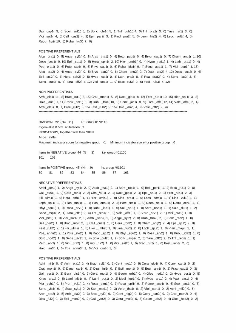
Sali _cap1( 3, 0) Scor _aut1( 5, 2) Sonc _ole1( 5, 1) Trif _dub1( 4, 0) Trif _pra1( 3, 0) Tuss _far1( 3, 0) Vici _sat1( 4, 0) Call _cus2( 4, 1) Epil _par2( 3, 1) Kind _pra2( 5, 0) Leon _his2( 4, 0) Leuc _vul2( 4, 0) Rubu _fru2( 10, 6) Rubu _fru3( 7, 0)
POSITIVE PREFERENTIALS
Alop _pra1( 0, 5) Ange _syl1( 0, 8) Arab _tha1( 0, 4) Betu _pub1( 0, 4) Bryu _cap1( 0, 7) Cham _ang1( 1, 10)
Desc _ces1( 0, 10) Epil _sp.1( 0, 5) Hera _sph1( 2, 10) Hier _umb1( 0, 4) Hypo _rad1( 1, 4) Lath _pra1( 0, 4) Poa_ prat1( 0, 6) Pote _ste1( 0, 5) Rhyt _squ1( 0, 6) Rubu _ida1( 0, 4) Sonc _asp1( 1, 7) Vici _sep1( 1, 13) Alop _pra2( 0, 4) Ange _syl2( 0, 5) Bryu _cap2( 0, 6) Cham _ang2( 0, 7) Dact _glo2( 4, 12) Desc _ces2( 0, 6) Epil _sp.2( 0, 5) Hera _sph2( 0, 5) Hypo _rad2( 0, 4) Lath _pra2( 0, 4) Poa_ prat2( 0, 4) Sene _jac2( 3, 8) Sonc _asp2( 0, 6) Tara _off2( 3, 12) Vici _sep2( 1, 9) Brac _rut3( 0, 6) Fest _rub3( 4, 12)
NON-PREFERENTIALS
Arrh _ela1( 11, 8) Brac _rut1( 8, 15) Crat _mon1( 5, 8) Dact _glo1( 8, 12) Fest _rub1( 10, 15) Hier _sp.1( 3, 3)
Holc _lan1( 7, 11) Ranu _acr1( 3, 3) Rubu _fru1( 10, 9) Sene _jac1( 8, 9) Tara _off1( 12, 14) Vale _off1( 2, 4) Arrh _ela2( 8, 7) Brac _rut2( 8, 15) Fest _rub2( 9, 15) Holc _lan2( 4, 9) Vale _off2( 2, 4)
************************************************************************************************************************
DIVISION 22 (N= 11) I.E. GROUP *0110 Eigenvalue 0.539 at iteration 3
INDICATORS, together with their SIGN
Ange _syl1(-)
Maximum indicator score for negative group -1 Minimum indicator score for positive group 0
Items in NEGATIVE group 44 (N= 2) i.e. group *01100 101 102
Items in POSITIVE group 45 (N= 9) i.e. group *01101
80 81 82 83 84 85 86 87 163
NEGATIVE PREFERENTIALS Ambl _ser1( 1, 0) Ange _syl1( 2, 0) Arab _tha1( 2, 1) Barb _rec1( 1, 0) Bell _per1( 1, 2) Brac _rut1( 2, 0)
Call _cus1( 1, 0) Cera _fon1( 2, 2) Cirs _vul1( 2, 1) Dact _glo1( 2, 4) Epil _sp.1( 2, 1) Fest _rub1( 2, 3) Fili _ulm1( 1, 0) Hera _sph1( 1, 1) Hier _umb1( 2, 0) Kind _pra1( 1, 0) Laps _com1( 1, 1) Lina _vul1( 2, 1) Loph _sp.1( 1, 0) Plan _maj1( 1, 1) Poa_ annu1( 2, 3) Pote _ste1( 1, 0) Raco _sp.1( 1, 0) Ranu _acr1( 1, 1) Rhyt _squ1( 1, 0) Rosa _arv1( 1, 0) Rubu _ida1( 1, 0) Sali _sp.1( 1, 0) Scro _nod1( 1, 1) Sola _dul1( 1, 2)
Sonc _asp1( 2, 4) Tara _off1( 2, 4) Trif _rep1( 1, 2) Vale _off1( 1, 0) Vero _arv1( 2, 1) Vici _cra1( 1, 0)
Vici _hir1( 1, 0) Vici _sat1( 2, 0) Ambl _ser2( 1, 0) Ange _syl2( 2, 0) Arab _tha2( 2, 0) Barb _rec2( 1, 0)
Bell _per2( 1, 0) Brac _rut2( 2, 0) Call _cus2( 1, 0) Cera _fon2( 1, 0) Cham _ang2( 2, 4) Epil _sp.2( 2, 0) Fest _rub2( 2, 1) Fili _ulm2( 1, 0) Hier _umb2( 1, 0) Lina _vul2( 2, 0) Loph _sp.2( 1, 0) Plan _maj2( 1, 1) Poa_ annu2( 2, 1) Pote _ste2( 1, 0) Raco _sp.2( 1, 0) Rhyt _squ2( 1, 0) Rosa _arv2( 1, 0) Rubu _ida2( 1, 0) Scro _nod2( 1, 0) Sene _jac2( 2, 4) Sola _dul2( 1, 2) Sonc _asp2( 2, 3) Tara _off2( 2, 2) Trif _rep2( 1, 1) Vero _arv2( 1, 0) Vici _cra2( 1, 0) Vici _hir2( 1, 0) Vici _sat2( 2, 0) Brac _rut3( 1, 0) Fest _rub3( 2, 0) Holc _lan3( 1, 0) Poa_ annu3( 2, 0) Vici _cra3( 1, 0)
POSITIVE PREFERENTIALS
Achi _mil1( 0, 6) Arrh _ela1( 0, 4) Brac _syl1( 0, 2) Cent _nig1( 0, 5) Cera _glo1( 0, 4) Cony _can1( 0, 2) Crat _mon1( 0, 6) Dauc _car1( 0, 2) Dips _ful1( 0, 3) Epil _mon1( 0, 5) Equi _arv1( 0, 2) Frax _exc1( 0, 3) Gali _ver1( 0, 3) Gera _dis1( 0, 2) Gera _mol1( 0, 4) Geum _urb1( 0, 4) Glec _hed1( 0, 2) Hype _per1( 0, 5) Knau _arv1( 0, 5) Lami _alb1( 0, 4) Lami _pur1( 0, 2) Medi _lup1( 0, 6) Myos _arv1( 0, 4) Past _sat1( 0, 4) Picr _ech1( 0, 5) Prun _vul1( 0, 4) Rosa _pim1( 0, 3) Rosa _spi1( 0, 3) Rume _ace1( 0, 6) Scor _aut1( 0, 8) Sene _vis1( 0, 4) Stac _syl1( 0, 2) Stel _med1( 0, 3) Verb _tha1( 0, 2) Viol _can1( 0, 2) Achi _mil2( 0, 6)
Aren _ser2( 0, 5) Arrh _ela2( 0, 3) Brac _syl2( 0, 2) Cent _nig2( 0, 5) Cony _can2( 0, 2) Crat _mon2( 0, 4)
Dips _ful2( 0, 3) Epil _mon2( 0, 2) Gali _ver2( 0, 3) Gera _mol2( 0, 3) Geum _urb2( 0, 4) Glec _hed2( 0, 2)

Hype _per2( 0, 3) Knau _arv2( 0, 5) Lami _alb2( 0, 4) Lami _pur2( 0, 2) Medi _lup2( 0, 6) Myos _arv2( 0, 3) Past _sat2( 0, 4) Pilo _off2( 0, 4) Rosa _pim2( 0, 2) Rosa _spi2( 0, 2) Rume _ace2( 0, 3) Scor _aut2( 0, 6) Sene _vis2( 0, 4) Verb _tha2( 0, 2) Vero _cha2( 0, 2) Medi _lup3( 0, 5) Rubu _fru3( 0, 3)
NON-PREFERENTIALS
Aren _ser1( 1, 5) Cham _ang1( 2, 5) Cirs _arv1( 1, 3) Holc _lan1( 1, 4) Leuc _vul1( 1, 5) Loli _per1( 1, 5)
Pilo _off1( 1, 4) Plan _lan1( 1, 4) Rubu _fru1( 2, 8) Sene _jac1( 2, 5) Urti _dio1( 1, 4) Vero _cha1( 1, 4) Dact _glo2( 1, 3) Holc _lan2( 1, 3) Leuc _vul2( 1, 5) Loli _per2( 1, 5) Plan _lan2( 1, 3) Rubu _fru2( 1, 7) ************************************************************************************************************************
DIVISION 23 (N= 5) I.E. GROUP *0111 Eigenvalue 0.266 at iteration 1
INDICATORS, together with their SIGN
Aira _car1(+)
Maximum indicator score for negative group 0 Minimum indicator score for positive group 1
Items in NEGATIVE group 46 (N= 3) i.e. group *01110 33 34 35
Items in POSITIVE group 47 (N= 2) i.e. group *01111
31 32
NEGATIVE PREFERENTIALS Agro _sto1( 1, 0) Anis _ste1( 2, 0) Cirs _arv1( 1, 0) Elyt _rep1( 1, 0) Hede _hel1( 1, 0) Poa_ prat1( 3, 1)
Poa_ prat1( 1, 0) Rosa _can1( 1, 0) Rume _ace1( 2, 0) Scor _aut1( 3, 0) Stel _med1( 1, 0) Succ _pra1( 1, 0) Tara _off1( 3, 0) Arte _vul2( 3, 1) Elyt _rep2( 1, 0) Leuc _vul2( 2, 0) Plan _lan2( 2, 0) Poa_ prat2( 2, 0) Poa_ prat2( 1, 0) Rume _ace2( 1, 0) Scor _aut2( 2, 0) Sene _jac2( 3, 1) Stel _med2( 1, 0) Tara _off2( 3, 0) Trif _cam2( 3, 1) Arrh _ela3( 1, 0) Dact _glo3( 1, 0)
POSITIVE PREFERENTIALS
Aira _car1( 0, 2) Desc _fle1( 0, 2) Hera _sph1( 0, 1) Hype _per1( 0, 1) Matr _dis1( 0, 1) Nard _str1( 0, 2) Sagi _pro1( 1, 2) Crep _cap2( 1, 2) Sagi _pro2( 0, 2) Rubu _fru3( 0, 2) Trif _cam3( 0, 1)
NON-PREFERENTIALS Achi _mil1( 3, 2) Arrh _ela1( 3, 2) Arte _vul1( 3, 2) Caly _sep1( 2, 2) Cham _ang1( 2, 1) Cony _can1( 3, 2)
Crep _cap1( 2, 2) Dact _glo1( 2, 2) Fest _rub1( 3, 2) Hypo _rad1( 1, 1) Leuc _vul1( 2, 1) Loli _per1( 3, 2)
Plan _lan1( 2, 1) Rubu _fru1( 2, 2) Sene _jac1( 3, 2) Trag _pra1( 2, 1) Trif _cam1( 3, 2) Achi _mil2( 3, 2)
Arrh _ela2( 3, 2) Caly _sep2( 2, 1) Cony _can2( 3, 2) Dact _glo2( 2, 2) Fest _rub2( 3, 2) Loli _per2( 3, 2)
Rubu _fru2( 2, 2) Achi _mil3( 3, 2) Fest _rub3( 2, 1) Loli _per3( 3, 2) ************************************************************************************************************************
DIVISION 24 (N= 4) I.E. GROUP *1000 DIVISION FAILS - There are too few items
************************************************************************************************************************
DIVISION 25 (N= 4) I.E. GROUP *1001
DIVISION FAILS - There are too few items
End of level 5
************************************************************************************************************************
DIVISION 32 (N= 2) I.E. GROUP *00000
DIVISION FAILS - There are too few items

************************************************************************************************************************
DIVISION 33 (N= 8) I.E. GROUP *00001 Eigenvalue 0.276 at iteration 3
INDICATORS, together with their SIGN
Brac _rut1(+)
Maximum indicator score for negative group 0 Minimum indicator score for positive group 1
Items in NEGATIVE group 66 (N= 5) i.e. group *000010 118 119 120 123 124
BORDERLINE negatives (N= 1)
118
Items in POSITIVE group 67 (N= 3) i.e. group *000011 115 116 117
NEGATIVE PREFERENTIALS Crep _ves1( 4, 0) Hype _per1( 3, 0) Medi _lup1( 2, 0) Sene _vis1( 4, 1) Stac _syl1( 2, 0) Vici _cra1( 2, 0)
Anth _syl2( 4, 1)
POSITIVE PREFERENTIALS
Anis _ste1( 0, 1) Arte _vul1( 1, 2) Brac _rut1( 0, 3) Cent _ery1( 2, 3) Cera _fon1( 2, 3) Cirs _arv1( 1, 2) Cirs _vul1( 0, 1) Cony _can1( 1, 3) Desc _ces1( 0, 1) Epil _par1( 0, 2) Equi _arv1( 0, 1) Gera _rob1( 0, 1) Hera _sph1( 1, 3) Leon _his1( 0, 2) Linu _cat1( 2, 3) Rese _lut1( 0, 1) Rubu _fru1( 1, 3) Rume _ace1( 0, 1) Rume _ace1( 0, 1) Rume _cri1( 0, 2) Sola _dul1( 1, 2) Anis _ste2( 0, 1) Arte _vul2( 0, 1) Brac _rut2( 0, 2) Cony _can2( 0, 2) Desc _ces2( 0, 1) Gali _apa2( 1, 3) Hera _sph2( 0, 1) Hypo _rad2( 1, 3) Pimp _sax2( 1, 2) Rubu _fru2( 0, 1) Rume _cri2( 0, 2) Sene _jac2( 0, 1) Tara _off2( 0, 1) Trag _pra2( 0, 1) Verb _tha2( 0, 1)
NON-PREFERENTIALS
Anth _syl1( 5, 2) Arrh _ela1( 5, 3) Cera _glo1( 1, 1) Dact _glo1( 4, 2) Epil _mon1( 3, 3) Epil _pal1( 1, 1) Gali _apa1( 4, 3) Hier _sp.1( 3, 2) Holc _lan1( 3, 2) Hypo _rad1( 3, 3) Picr _ech1( 4, 2) Pimp _sax1( 3, 2) Sene _jac1( 4, 3) Sonc _asp1( 5, 3) Tara _off1( 5, 3) Trag _pra1( 1, 1) Verb _tha1( 2, 2) Vero _arv1( 3, 2) Vulp _bro1( 5, 3) Arrh _ela2( 5, 3) Cirs _arv2( 1, 1) Dact _glo2( 3, 1) Holc _lan2( 2, 2) Picr _ech2( 1, 1) Sonc _asp2( 2, 2) Vulp _bro2( 5, 3) Arrh _ela3( 3, 1) Vulp _bro3( 3, 3)
************************************************************************************************************************
DIVISION 34 (N= 19) I.E. GROUP *00010
Eigenvalue 0.347 at iteration 7 INDICATORS, together with their SIGN Fest _rub2(-) Rubu _fru1(-) Maximum indicator score for negative group -2 Minimum indicator score for positive group -1
Items in NEGATIVE group 68 (N= 6) i.e. group *000100
47 170 171 172 173 174
Items in POSITIVE group 69 (N= 13) i.e. group *000101 131 134 144 145 146 147 148 149 150 151 152 153
169
BORDERLINE positives (N= 1) 169
NEGATIVE PREFERENTIALS

Bryu _cap1( 5, 2) Cent _nig1( 3, 1) Cera _fon1( 2, 2) Cirs _arv1( 5, 4) Cirs _vul1( 2, 0) Crat _mon1( 2, 0) Dact _glo1( 6, 3) Echi _vul1( 4, 0) Epil _hir1( 2, 0) Epil _mon1( 6, 6) Erig _ace1( 2, 0) Fest _rub1( 6, 3) Frax _exc1( 2, 0) Hier _sp.1( 5, 2) Hype _per1( 3, 0) Lact _ser1( 3, 0) Linu _cat1( 3, 1) Picr _ech1( 3, 0) Pote _rep1( 3, 0) Rese _lut1( 4, 1) Rubu _fru1( 6, 2) Sonc _asp1( 5, 4) Verb _tha1( 4, 0) Cent _nig2( 2, 1)
Dact _glo2( 5, 1) Echi _vul2( 4, 0) Erig _ace2( 2, 0) Fest _rub2( 6, 1) Hier _sp.2( 2, 0) Hype _per2( 2, 0)
Lact _ser2( 2, 0) Lina _vul2( 5, 5) Plan _maj2( 2, 0) Rese _lut2( 4, 1) Rubu _fru2( 5, 0) Tana _vul2( 5, 3)
Verb _tha2( 4, 0)
POSITIVE PREFERENTIALS Agro _sto1( 0, 5) Anis _ste1( 1, 5) Betu _pub1( 1, 7) Cera _pur1( 0, 6) Desc _ces1( 2, 11) Hypo _rad1( 0, 4)
Sagi _pro1( 0, 4) Sali _cap1( 0, 3) Scor _aut1( 0, 4) Sene _jac1( 1, 10) Anis _ste2( 0, 3) Cera _pur2( 0, 5) Desc _ces2( 0, 10) Equi _arv2( 0, 3) Sene _jac2( 0, 4)
NON-PREFERENTIALS
Agro _cap1( 3, 11) Arrh _ela1( 5, 12) Betu _pen1( 5, 10) Bryu _arg1( 2, 7) Cham _ang1( 6, 10) Epil _pal1( 4, 8) Epil _par1( 6, 11) Equi _arv1( 2, 5) Hera _sph1( 2, 4) Holc _lan1( 5, 9) Leon _his1( 2, 3) Lina _vul1( 5, 11) Plan _maj1( 4, 8) Tana _vul1( 5, 7) Tara _off1( 5, 9) Vulp _bro1( 5, 11) Agro _cap2( 2, 5) Arrh _ela2( 4, 10) Betu _pen2( 4, 6) Cham _ang2( 3, 5) Holc _lan2( 5, 8) Vulp _bro2( 5, 6)
************************************************************************************************************************
DIVISION 35 (N= 5) I.E. GROUP *00011
Eigenvalue 0.654 at iteration 1
INDICATORS, together with their SIGN Acer _pse1(+)
Maximum indicator score for negative group 0 Minimum indicator score for positive group 1
Items in NEGATIVE group 70 (N= 4) i.e. group *000110 57 58 59 60
Items in POSITIVE group 71 (N= 1) i.e. group *000111
110
NEGATIVE PREFERENTIALS Agro _sto1( 1, 0) Anag _arv1( 1, 0) Aspl _rut1( 1, 0) Brac _rut1( 3, 0) Cirs _arv1( 1, 0) Crat _mon1( 1, 0)
Gali _mol1( 1, 0) Glec _hed1( 1, 0) Hera _sph1( 3, 0) Merc _per1( 3, 0) Plan _maj1( 3, 0) Prim _vul1( 2, 0) Rume _ace1( 1, 0) Sonc _asp1( 3, 0) Stel _med1( 2, 0) Tara _off1( 2, 0) Urti _dio1( 3, 0) Vero _arv1( 3, 0)
Vici _sat1( 3, 0) Brac _rut2( 1, 0) Cham _ang2( 1, 0) Loli _per2( 2, 0) Arrh _ela3( 4, 0)
POSITIVE PREFERENTIALS Acer _pse1( 0, 1) Agro _cap1( 1, 1) Betu _pen1( 0, 1) Budd _dav1( 0, 1) Call _cus1( 0, 1) Conv _arv1( 1, 1)
Dips _ful1( 0, 1) Epil _mon1( 2, 1) Epil _par1( 0, 1) Fest _rub1( 0, 1) Gera _dis1( 0, 1) Geum _urb1( 1, 1) Hede _hel1( 0, 1) Holc _lan1( 1, 1) Hype _pul1( 0, 1) Hypo _rad1( 0, 1) Laps _com1( 0, 1) Leon _his1( 0, 1) Plan _lan1( 0, 1) Prun _vul1( 0, 1) Rhyt _squ1( 0, 1) Sagi _pro1( 1, 1) Trag _pra1( 0, 1) Trif _cam1( 0, 1) Trif _dub1( 0, 1) Vici _hir1( 0, 1) Vulp _bro1( 0, 1) Betu _pen2( 0, 1) Budd _dav2( 0, 1) Holc _lan2( 0, 1)
Leon _his2( 0, 1) Rhyt _squ2( 0, 1) Trif _dub2( 0, 1) Vici _hir2( 0, 1) Vulp _bro2( 0, 1) Budd _dav3( 0, 1)
NON-PREFERENTIALS Arrh _ela1( 4, 1) Cera _pur1( 4, 1) Cham _ang1( 4, 1) Loli _per1( 3, 1) Poa_ annu1( 4, 1) Rubu _fru1( 4, 1)
Sene _jac1( 4, 1) Arrh _ela2( 4, 1) Cera _pur2( 4, 1) ************************************************************************************************************************
DIVISION 36 (N= 10) I.E. GROUP *00100
Eigenvalue 0.486 at iteration 3
INDICATORS, together with their SIGN
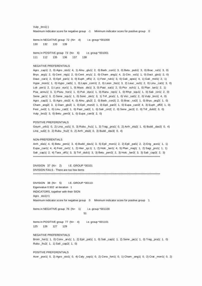
Vulp _bro1(-) Maximum indicator score for negative group -1 Minimum indicator score for positive group 0
Items in NEGATIVE group 72 (N= 4) i.e. group *001000
130 132 133 139
Items in POSITIVE group 73 (N= 6) i.e. group *001001 111 112 135 136 137 138
NEGATIVE PREFERENTIALS Agro _cap1( 2, 0) Agro _sto1( 4, 1) Alnu _glu1( 2, 0) Barb _con1( 3, 0) Betu _pub1( 3, 0) Brac _rut1( 3, 0)
Bryu _arg1( 2, 0) Cent _nig1( 2, 0) Cent _ery1( 2, 0) Cham _ang1( 4, 2) Cirs _vul1( 1, 0) Dact _glo1( 2, 0)
Dauc _car1( 2, 0) Epil _par1( 3, 0) Euph _off1( 2, 1) Fest _rub1( 3, 0) Gali _apa1( 4, 1) Gali _mol1( 2, 1)
Hype _mon1( 1, 0) Hypo _rad1( 1, 0) Laps _com1( 2, 0) Leon _his1( 3, 2) Leuc _vul1( 2, 0) Linu _cat1( 3, 0)
Loli _per1( 2, 1) Lyco _eur1( 1, 0) Myos _dis1( 3, 0) Past _sat1( 2, 0) Picr _ech1( 1, 0) Plan _lan1( 2, 1) Poa_ annu1( 3, 1) Pseu _hor1( 1, 0) Puli _dys1( 1, 0) Ranu _rep1( 1, 0) Rhyt _squ1( 1, 0) Sali _cin1( 2, 0) Sene _jac1( 3, 2) Sene _squ1( 1, 0) Sonc _ole1( 3, 1) Trif _pra1( 1, 0) Vici _sat1( 2, 0) Vulp _bro1( 4, 0) Agro _cap2( 1, 0) Agro _sto2( 4, 0) Alnu _glu2( 2, 0) Barb _con2( 2, 0) Brac _rut2( 1, 0) Bryu _arg2( 1, 0) Cham _ang2( 3, 1) Dact _glo2( 1, 0) Epil _mon2( 1, 0) Epil _par2( 1, 0) Eupa _can2( 4, 3) Euph _off2( 1, 0) Fest _ovi2( 1, 0) Linu _cat2( 1, 0) Past _sat2( 1, 0) Sali _cin2( 2, 0) Sene _jac2( 2, 0) Trif _dub2( 3, 0)
Vulp _bro2( 3, 0) Betu _pen3( 1, 0) Eupa _can3( 2, 0)
POSITIVE PREFERENTIALS Geum _urb1( 0, 2) Lina _vul1( 0, 3) Rubu _fru1( 1, 3) Trag _pra1( 0, 2) Arrh _ela2( 1, 6) Budd _dav2( 0, 4)
Lina _vul2( 0, 2) Rubu _fru2( 0, 2) Arrh _ela3( 0, 3) Budd _dav3( 0, 4)
NON-PREFERENTIALS Arrh _ela1( 4, 6) Betu _pen1( 3, 4) Budd _dav1( 3, 5) Epil _mon1( 2, 2) Epil _pal1( 2, 2) Erig _ace1( 1, 1)
Eupa _can1( 4, 4) Fest _ovi1( 1, 2) Hier _sp.1( 1, 2) Holc _lan1( 4, 5) Plan _maj1( 1, 2) Sagi _pro1( 1, 1)
Sali _cap1( 2, 4) Tara _off1( 3, 3) Trif _dub1( 3, 3) Betu _pen2( 2, 3) Holc _lan2( 3, 3) Sali _cap2( 2, 3)
************************************************************************************************************************
DIVISION 37 (N= 2) I.E. GROUP *00101 DIVISION FAILS - There are too few items
************************************************************************************************************************
DIVISION 38 (N= 5) I.E. GROUP *00110
Eigenvalue 0.502 at iteration 1
INDICATORS, together with their SIGN Agro _sto1(+)
Maximum indicator score for negative group 0 Minimum indicator score for positive group 1
Items in NEGATIVE group 76 (N= 1) i.e. group *001100 51
Items in POSITIVE group 77 (N= 4) i.e. group *001101
125 126 127 129
NEGATIVE PREFERENTIALS Brom _hor1( 1, 0) Conv _arv1( 1, 2) Epil _pal1( 1, 0) Sali _cap1( 1, 2) Sene _jac1( 1, 0) Trag _pra1( 1, 0)
Rubu _fru2( 1, 1) Sali _cap2( 1, 0)
POSITIVE PREFERENTIALS
Acer _pse1( 0, 2) Agro _sto1( 0, 4) Caly _sep1( 0, 2) Cera _fon1( 0, 1) Cham _ang1( 0, 2) Crat _mon1( 0, 2)

Epil _hir1( 0, 2) Epil _sp.1( 0, 1) Eupa _can1( 0, 3) Fest _ovi1( 0, 4) Gera _rob1( 0, 1) Holc _lan1( 0, 4) Lina _vul1( 0, 1) Medi _lup1( 0, 1) Plan _lan1( 0, 1) Poa_ annu1( 0, 1) Prun _sp.1( 0, 1) Rume _cri1( 0, 2) Sagi _pro1( 0, 1) Sali _cin1( 0, 3) Sene _squ1( 0, 3) Sonc _asp1( 0, 3) Stac _syl1( 0, 3) Vici _cra1( 0, 2) Agro _sto2( 0, 1) Caly _sep2( 0, 1) Conv _arv2( 0, 1) Epil _hir2( 0, 2) Epil _par2( 0, 1) Eupa _can2( 0, 1)
Medi _lup2( 0, 1)
NON-PREFERENTIALS Arrh _ela1( 1, 4) Epil _par1( 1, 3) Rubu _fru1( 1, 4) Tara _off1( 1, 3) Arrh _ela2( 1, 3) Arrh _ela3( 1, 3)
************************************************************************************************************************
DIVISION 39 (N= 5) I.E. GROUP *00111 Eigenvalue 0.442 at iteration 1
INDICATORS, together with their SIGN
Lotu _cor1(-)
Maximum indicator score for negative group -1 Minimum indicator score for positive group 0
Items in NEGATIVE group 78 (N= 3) i.e. group *001110 128 140 141
Items in POSITIVE group 79 (N= 2) i.e. group *001111
142 143
NEGATIVE PREFERENTIALS Betu _pub1( 1, 0) Caly _sep1( 1, 0) Cent _ery1( 1, 0) Cera _fon1( 3, 1) Cham _ang1( 1, 0) Conv _arv1( 1, 0)
Crep _cap1( 1, 0) Desc _ces1( 1, 0) Fest _ovi1( 3, 1) Gali _apa1( 1, 0) Hype _per1( 1, 0) Hypo _rad1( 2, 0) Laps _com1( 1, 0) Lotu _cor1( 3, 0) Plan _lan1( 2, 0) Plan _maj1( 1, 0) Rosa _can1( 1, 0) Sagi _pro1( 1, 0) Sali _cap1( 1, 0) Soli _can1( 1, 0) Tara _off1( 3, 1) Trif _dub1( 2, 0) Trif _pra1( 1, 0) Tuss _far1( 2, 0) Agro _sto2( 3, 1) Lotu _cor2( 1, 0) Agro _sto3( 2, 0) Arrh _ela3( 1, 0)
POSITIVE PREFERENTIALS
Budd _dav1( 0, 1) Cirs _arv1( 0, 1) Epil _par1( 0, 1) Gera _rob1( 0, 1) Medi _lup1( 0, 1) Oeno _cam1( 0, 1) Poa_ prat1( 0, 2) Rume _cri1( 0, 1) Scro _nod1( 0, 2) Sola _dul1( 0, 1) Stac _syl1( 1, 2) Arte _vul2( 0, 1) Equi _arv2( 0, 1) Euph _off2( 0, 1) Medi _lup2( 0, 1) Rubu _fru2( 1, 2) Tara _off2( 0, 1) Trif _rep2( 0, 1) Euph _off3( 0, 1) Holc _lan3( 0, 1) Medi _lup3( 0, 1) Rubu _fru3( 0, 1)
NON-PREFERENTIALS
Agro _sto1( 3, 2) Arrh _ela1( 2, 2) Arte _vul1( 1, 1) Epil _cil1( 1, 1) Epil _hir1( 2, 1) Equi _arv1( 1, 1)
Eupa _can1( 3, 2) Euph _off1( 1, 1) Hier _umb1( 1, 1) Holc _lan1( 3, 2) Ranu _rep1( 1, 1) Rubu _fru1( 2, 2)
Sali _cin1( 1, 1) Sonc _asp1( 2, 2) Trif _rep1( 1, 1) Vici _hir1( 1, 1) Arrh _ela2( 2, 1) Epil _hir2( 1, 1) Eupa _can2( 3, 2) Fest _ovi2( 1, 1) Holc _lan2( 2, 1) Sali _cin2( 1, 1) Eupa _can3( 3, 2)
************************************************************************************************************************
DIVISION 40 (N= 17) I.E. GROUP *01000 Eigenvalue 0.526 at iteration 4
INDICATORS, together with their SIGN
Sene _jac1(+) Rubu _fru2(+) Cham _ang1(-) Gera _rob3(-) Hede _hel1(+)
Maximum indicator score for negative group 0 Minimum indicator score for positive group 1
Items in NEGATIVE group 80 (N= 7) i.e. group *010000 23 157 158 159 160 161 166
Items in POSITIVE group 81 (N= 10) i.e. group *010001
1 2 3 4 5 28 29 30 107 108

NEGATIVE PREFERENTIALS Bryu _cap1( 3, 2) Call _vul1( 3, 1) Cham _ang1( 6, 0) Epil _cil1( 6, 3) Epil _tet1( 4, 0) Frag _ves1( 3, 0)
Gera _mol1( 2, 0) Geum _riv1( 4, 0) Geum _urb1( 3, 1) Lath _pra1( 3, 0) Lotu _cor1( 4, 1) Prun _vul1( 2, 1) Quer _rob1( 2, 0) Rhyt _squ1( 2, 1) Sonc _ole1( 2, 0) Vici _oro1( 2, 0) Cham _ang2( 5, 0) Epil _cil2( 5, 1)
Epil _tet2( 4, 0) Gera _rob2( 5, 1) Lotu _cor2( 4, 0) Arrh _ela3( 6, 2) Gera _rob3( 5, 0) Lotu _cor3( 2, 0)
POSITIVE PREFERENTIALS Agro _cap1( 2, 6) Agro _sto1( 0, 3) Anth _odo1( 0, 5) Atri _und1( 0, 3) Brac _rut1( 0, 6) Camp _int1( 0, 4)
Dact _glo1( 1, 6) Epil _hir1( 0, 3) Epil _par1( 0, 4) Equi _arv1( 1, 3) Frax _exc1( 1, 5) Hede _hel1( 0, 7) Lina _vul1( 1, 3) Moli _cae1( 0, 3) Plan _lan1( 2, 8) Poly _com1( 1, 4) Schi _cra1( 0, 3) Sene _jac1( 0, 9) Tara _off1( 0, 3) Agro _cap2( 0, 5) Anth _odo2( 0, 5) Brac _rut2( 0, 4) Dact _glo2( 0, 4) Fest _rub2( 1, 3) Frax _exc2( 0, 5) Hede _hel2( 0, 6) Moli _cae2( 0, 3) Plan _lan2( 1, 5) Poly _com2( 1, 3) Rubu _fru2( 0, 9)
Anth _odo3( 0, 5) Moli _cae3( 0, 3) Rubu _fru3( 0, 3)
NON-PREFERENTIALS Arrh _ela1( 7, 8) Fest _rub1( 3, 7) Gera _rob1( 5, 7) Holc _lan1( 7, 9) Loli _per1( 5, 5) Rubu _fru1( 4, 9)
Arrh _ela2( 7, 6) Holc _lan2( 7, 9) Loli _per2( 2, 3) Holc _lan3( 2, 3) ************************************************************************************************************************
DIVISION 41 (N= 43) I.E. GROUP *01001
Eigenvalue 0.344 at iteration 20
INDICATORS, together with their SIGN
Agro _cap1(-) Epil _mon1(+) Hypn _cup1(-) Arrh _ela3(+) Rubu _fru2(+) Brac _rut1(+) Bryo _rec1(+) Maximum indicator score for negative group 1 Minimum indicator score for positive group 2
Items in NEGATIVE group 82 (N= 24) i.e. group *010010 17 18 19 20 21 22 24 25 26 27 36 37
38 39 40 41 42 43 44 45 69 71 74 99
Items in POSITIVE group 83 (N= 19) i.e. group *010011
52 53 54 55 56 61 62 63 72 76 77 78 79 109 113 114 165 167 168
MISCLASSIFIED positives (N= 1) 72
NEGATIVE PREFERENTIALS
Agro _cap1( 18, 1) Dact _glo1( 10, 2) Epil _cil1( 7, 0) Epil _hir1( 5, 0) Gera _rob1( 10, 1) Hera _sph1( 7, 0)
Hypn _cup1( 14, 0) Hypo _rad1( 5, 0) Impa _gla1( 6, 0) Quer _rob1( 5, 1) Sonc _asp1( 5, 1) Sorb _auc1( 5, 0) Teuc _sco1( 6, 0) Viol _riv1( 6, 0) Fest _rub2( 13, 5) Hypn _cup2( 11, 0) Frax _exc3( 6, 1)
POSITIVE PREFERENTIALS Brac _rut1( 0, 7) Bryo _rec1( 0, 7) Budd _dav1( 2, 4) Elyt _rep1( 0, 4) Epil _mon1( 0, 12) Equi _arv1( 2, 5)
Geum _urb1( 2, 6) Poa_ prat1( 0, 4) Rhyt _squ1( 1, 5) Brac _rut2( 0, 4) Elyt _rep2( 0, 4) Equi _arv2( 0, 4)
Arrh _ela3( 9, 18)
NON-PREFERENTIALS Arrh _ela1( 23, 19) Betu _pen1( 5, 2) Cham _ang1( 10, 7) Fest _rub1( 17, 9) Frax _exc1( 9, 6) Holc _lan1( 4, 4)
Plan _lan1( 5, 2) Rubu _fru1( 17, 19) Sene _jac1( 12, 6) Tara _off1( 14, 6) Arrh _ela2( 19, 19) Cham _ang2( 6, 4) Frax _exc2( 7, 5) Rubu _fru2( 13, 18) Rubu _fru3( 7, 7)
************************************************************************************************************************