the physics of counting and sampling on random instances lenka … · 2020-01-03 · the physics of...
TRANSCRIPT

THE PHYSICS OFCOUNTING AND SAMPLING ON
RANDOM INSTANCES
Lenka Zdeborová(CEA Saclay and CNRS, France)
Monday, February 1, 16

MAIN CONTRIBUTORS TO THE PHYSICS UNDERSTANDING OF RANDOM INSTANCES
Braunstein, Franz, Kabashima, Kirkpatrick, Krzakala, Monasson, Montanari, Nishimori, Pagnani, Parisi, Ricci-Tersenghi, Saad, Semerjian, Sherrington, Sourlas, Sompolinsky, Tanaka, Weigt, Zdeborova, Zecchina, ....
Monday, February 1, 16

WHY RANDOM?
First step towards “typical” instances.
Intriguing mathematical properties
Solvable (by theoretical physics standards, mean field ...). Using belief propagation, Bethe approximation and its extensions, cavity method, replica symmetry breaking.
Ideas, inspiration and benchmarks for algorithms
also Andrea’s talk
Monday, February 1, 16
THE PICTURE
This talk’s example: Graph coloring on random graphs.
Resulting picture relevant for: satisfiability, CSP, vertex cover, independent sets, max-cut, .... error correcting codes, sparse estimation, regression, clustering, compressed sensing, feature learning, neural networks, ....
Monday, February 1, 16

GRAPH COLORING
How many proper colorings on a large random graph?
Can they be sampled uniformly? MCMC properties?
Variant 1: Finite temperature
Variant 2: Planted graphs Fix a random string of colors {s⇤i }i=1,...,N
s⇤i = s⇤j ) (ij) /2 E
µ({si}i=1,...,N ) =1
ZG(�)e��
P(ij)2E �si,sj
also Andrea’s talk
Monday, February 1, 16

COUNTING COLORINGS
Annealed entropy
Quenched entropy
sann = lim
N!1
1
N[logE(ZG)] = log q +
c
2
log 1� 1
q
s = lim
N!1
1
NE[log (ZG + 1)]
c fixed, N ! 1,|V | = N, |E| = M, c = 2M/N
Averaging and the large N limit.
Monday, February 1, 16

COUNTING COLORINGS
c fixed, N ! 1,
s = lim
N!1
1
NE[log (ZG + 1)]
|V | = N, |E| = M, c = 2M/N
sann = lim
N!1
1
N[logE(ZG)] = log q +
c
2
log (1� 1
q)
cc: colorability threshold
cK: Kauzmann/condensation
s < sann for c > cK
s = 0 for c > cc
(Krzakala et al. PNAS’07)
Monday, February 1, 16

PHASE TRANSITIONS
cu cd cK cc
cc: colorability threshold
cK: Kauzmann/condensation transition
cd: dynamical/clustering/reconstruction transition
cu: unicity threshold
sometimes (e.g. 3-SAT or 3-coloring) cK= cd
Monday, February 1, 16

SAMPLING
cluster = blue blob = subspace
that MCMC samples
uniformly in linear time.
⌃ = lim
N!1
1
NE[log (#clusters)]
Recall: random graph, random or warm start, weaker convergence that total variation.
cu cd cK cc
q ! 1 ⇡ q log q ⇡ 2q log q⇡ q
Monday, February 1, 16

TEMPERATURE DEPENDENCE
liquid
ideal glassdynamical glass
liquid
Monday, February 1, 16

TEMPERATURE DEPENDENCE
liquid
ideal glassdynamical glass
liquid
sampling easy
sampling hard
Monday, February 1, 16

WHAT IS A PHASE TRANSITION?
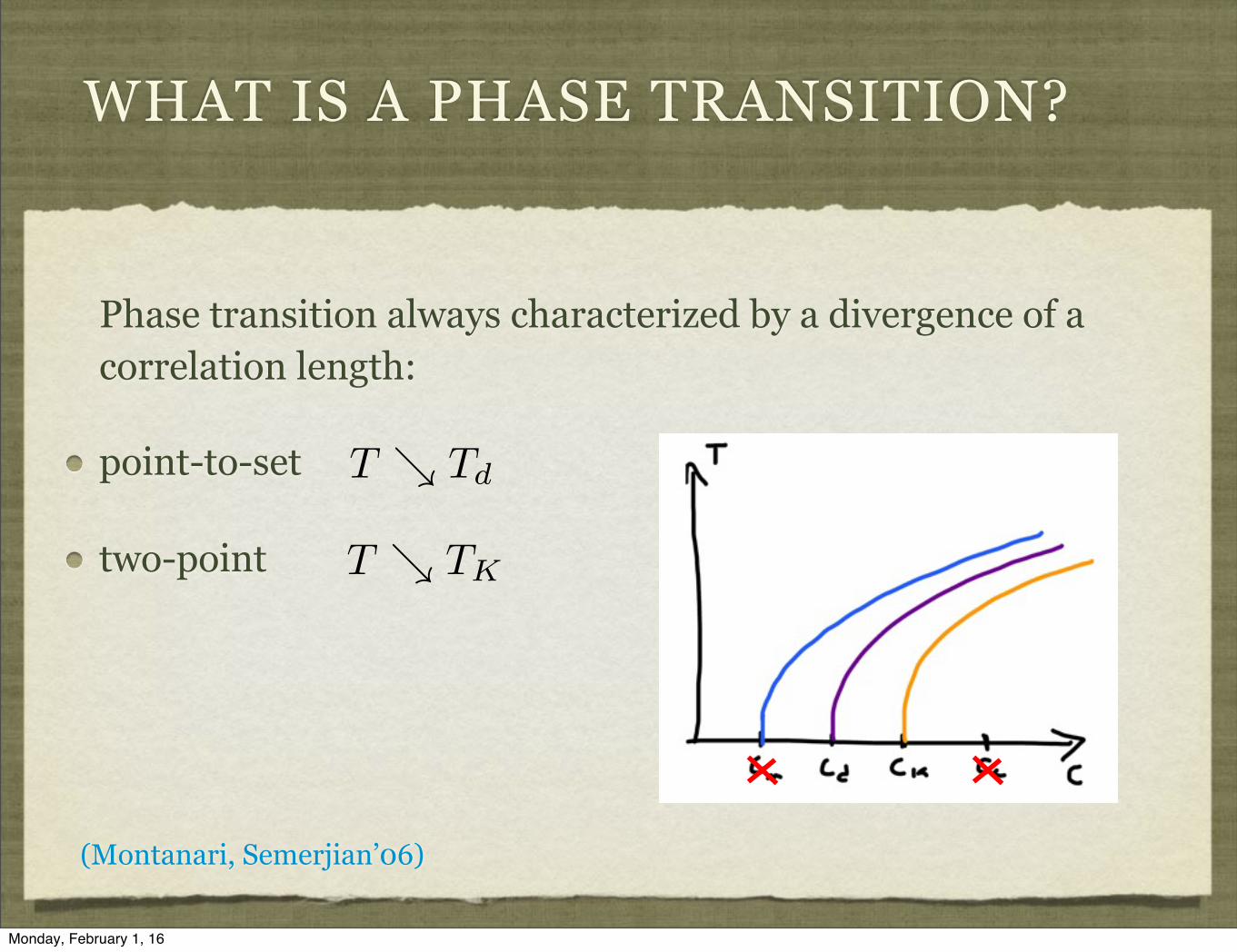
Phase transition always characterized by a divergence of a correlation length:
point-to-set
two-point
T & Td
T & TK
(Montanari, Semerjian’06)
Monday, February 1, 16
WHAT IS A PHASE TRANSITION?
Phase transition always characterized by a divergence of a correlation length:
point-to-set
two-point
T & Td
T & TK
(Montanari, Semerjian’06)
Monday, February 1, 16

PLANTED COLORING
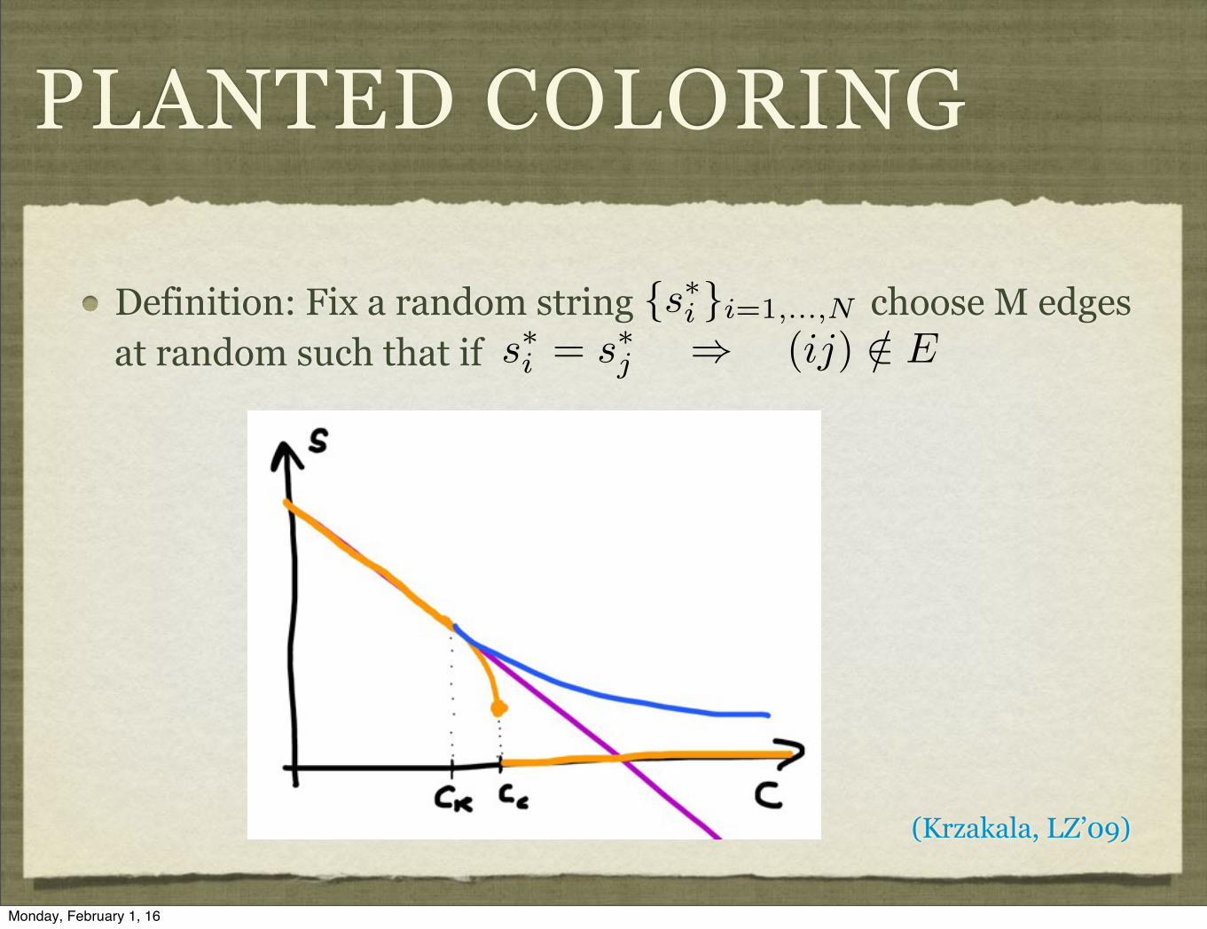
Definition: Fix a random string choose M edges at random such that if
Interest n.1 = paradigm of statistical inference (95% of use of MCMC in computer science). Bayes optimal inference = computing marginals of the posterior distribution = approximate counting problem.
Interest n.2 = Math simpler. “Warm start” for MCMC for free.
{s⇤i }i=1,...,N
s⇤i = s⇤j ) (ij) /2 E
also Andrea’s talk
Monday, February 1, 16
Definition: Fix a random string choose M edges at random such that if
{s⇤i }i=1,...,N
(Krzakala, LZ’09)
PLANTED COLORING
s⇤i = s⇤j ) (ij) /2 E
Monday, February 1, 16
PLANTED PHASE TRANSITIONS
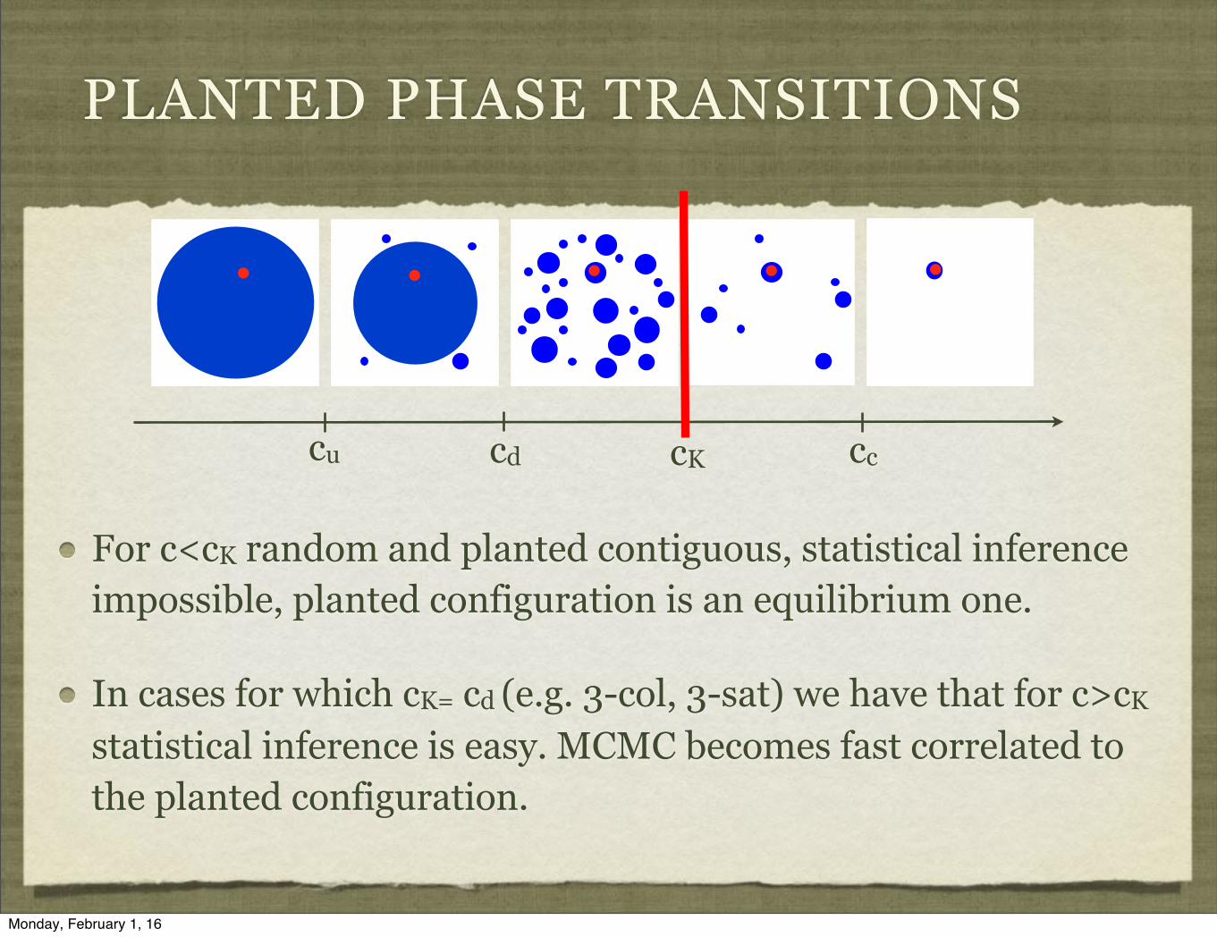
For c<cK random and planted contiguous, statistical inference impossible, planted configuration is an equilibrium one.
In cases for which cK= cd (e.g. 3-col, 3-sat) we have that for c>cK statistical inference is easy. MCMC becomes fast correlated to the planted configuration.
cu cd cK cc
Monday, February 1, 16

PLANTED PHASE TRANSITIONS
For c<cK random and planted contiguous, statistical inference impossible, planted configuration is an equilibrium one.
“spinodal” phase transition at
‣ evaluation of marginals (inference, sampling) hard
‣ evaluation of marginals tractable
cu cd cK cc
cK < c < csc > cs
cs
cs
q ! 1 ⇡ q log q ⇡ 2q log q⇡ q ⇡ q2
Monday, February 1, 16

1ST ORDER TRANSITION
0
0.2
0.4
0.6
0.8
1
12 13 14 15 16 17 18
over
lap
c
q=5,cin=0, N=100k
cd cs
init. plantedinit. random
planted 5-coloring
overlap
logZ
Monday, February 1, 16
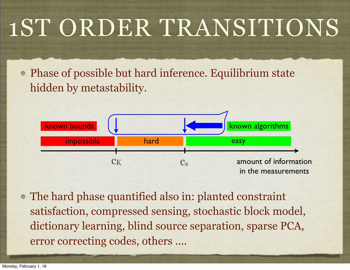
1ST ORDER TRANSITIONS
Phase of possible but hard inference. Equilibrium state hidden by metastability.
The hard phase quantified also in: planted constraint satisfaction, compressed sensing, stochastic block model, dictionary learning, blind source separation, sparse PCA, error correcting codes, others ....
amount of information in the measurements
easyhardimpossible
known bounds known algorithms
cK cs
Monday, February 1, 16

THE BIG QUESTION
Establish rigorous notions of algorithmic complexity (some kind of dichotomies) that are sensitive to the dynamical (cd) and the spinodal (cs) phase transition.
Monday, February 1, 16