THE PESTICIDE CONTAMINATION PREVENTION ACT: SETTING SPECIFIC NUMERICAL VALUES

bY

M.R. Wilkerson and K.D. Kim

December 1, 1986

ENVIRONMENTAL HAZARDS ASSESSMENT PROGRAM

.

EH 86-02

SUMMARY The Pesticide Contamination Prevention Act (PCPA) (Food and Agricultural Code,

Division 7, Chapter 2, Article 15, Section 13144) requires the California

Department of Food and Agriculture (CDFA) to establish specific numerical values

(SNVs) for water solubility, soil adsorption coefficient (Koc), hydrolysis

half-life, aerobic and anaerobic soil metabolism and field dissipation of

pesticides by December 1, 1986*. Pesticides whose environmental fate properties

exceed the SNVs must be reported to the State Legislature by December 1, 1987 and

may be subject to further regulation if their agricultural use practices increase

the probability that these pesticides will contaminate ground water.

SNVs were calculated using a method that is quantitative, reproducible and

verifiable by historical detection data while adhering to PCPA requirements. The

procedure for calculating SNVs was accomplished in two phases. In the initial

phase, pesticide monitoring studies were performed to determinewhichpesticides

had been detected in ground water as a result. of agricultural use, and which

pesticides have not yet been detected in ground water. Next, values for the

environmental fate variables required by the PCPA were collected from published

literature for over 200 active ingredients. The collected data were then entered

into a data base management system for future statistical analysis.

The final phase involved evaluation and selectlon of mathematical and statistical

methods that could be used to determine the most appropriate criteria for

identifying potential ground water pollutants. The primary concern in setting

values was that the final values should correctly classi.fy pesticides according

to their actual presence or absence in ground water. Therefore, a method of

calculating SNVs was chosen based on a comparison of environmental fate values of

common contaminants with those of non-contaminants. Comparison of environmental

fate values of contaminant and non-contaminant pesticides revealed that while

there are significant differences in the Koc and water solubility between the two

-_I,---I_--- ------.--we ------------.---- -----.----I--.-- ----.--------

*While collecting values on environmental fate properties, it became apparent that sufficient data for independent values of aerobic and anaerobic metabolism or field dissipation did not exist. Consequently, these categories have been grouoed together and represented by an SNV for soildegradationhalf-life.

pesticide groups, there are no significant differences between the hydrolysis and

soil degradation half-lives of the two groups.

Based on available data, CDFA has determined that pesticides with the following

average values may be classified as potential ground water contaminants :

A. Soil adsorption coefficient (Koc) less than 512 cm3/ gm or water s,olubility

gre,ater than 7 parts per million, and

B. Hydrolysis half-life greater than 13 days or soil

greater than 11 days.

degradation half-life

These values and the methods by which they were derived were reviewed by

consultants from the University of California. The values are more stringent

than criteria currently used by the U.S. Environmental Protection Agency for Koc

(300-500 cm3/gm), water solubility (30 ppm), hydrolysis half-life (25 weeks) or

,soil degradation half-life (2-3 weeks).

CDFA efforts to calculate SNVs were hampered by a lack of environmental fate data

for many pesticides. and ,by a general tendency to report the details of only

pos+tive detections when ground water surveys were conducted. Mor,e standardized

data should be available after the ,PCPA environmental fate data collection

process is completed. As provided for in the PCPA, the SNVs now proposed should

,be revised to imp.rove their ability, to i$ent,ify ground water contaminants as

additional data, become available, and, before the SNVs are, used to ,prepare .t.he

,annua) lists off potential ground water Contaminants. : ‘.

: .t i

! /

i

ii

ACKNOWLEDGEHENT

The author is indebted to Dr. Walter Farmer, Department of Soil Science,

University of California, RIverside and Dr. Jim Seiber, Department of

Environmental Toxicology, University of California, Davis for generous advice

and the critical review of materials and methods used in preparing this report.

The independent comments of these scientists are attached as an appendix. Dr.

William Jury, Department of Soil Science, University of California, Riverside and

Dr. William Spencer, USDA Soil Salinity Laboratory, University of California,

Riverside also contributed many comments during the course of this work and their

time and effort is greatly appreciated. The results presented do not necessarily

represent the views of any of the persons acknowledged above.

iii

iv

FIGURES Page

Figure 1. Stylized distributions of log Koc and log water solubility values of contaminant and non-contam- inant pesticide groups based upon group means and standard deviations. . . . . . . . . . . . . . . ..*................. 9

Figure 2. Stylized distributions of log hydrolysis half-life and log soil degradation half-life of contaminant, non-contaminant, and combined pesticide groups based on group means and standard deviations. . . . . . . . . 10

V

THE PESTICIDE CONTAMINATION PREVENTION ACT: SETTING SPECIFIC NUMERICAL VALUES

INTRODUCTION

This report summarizes a procedure to set specific numerical values for certain

pesticide properties as required by the PesticFde Contamination Prevention Act,

Food and Agricultural Code, Division 7, Chapter 2, Article 15, Section 13144.

Section 13144 requires that the California Department of Food and Agriculture

(CDFA) establish specific numerical values (SNVs) for water solubility, soil

adsorption coefficient (Koc), hydrolysis, aerobic and anaerobic soil metabolism,

and field dissipation. Pesticides whose chemical properties exceed the SNVs will

be reported to the State Legislature, and may later be placed upon a Ground Water

Protection List depending upon whether their registered use practices present a

risk of ground water contamination.

Three activities occurred in the initial phase of setting SNVs. First, a survey

of ground water quality studies was conducted to identify pesticides and

pesticide breakdown products which have been detected in ground water as a result

of agricultural use in the United States, as well as those which have been

monitored for, but not detected, in areas where use was known to occur. Secondly,

data for environmental fate properties of over 200 pesticide active ingredients

were collected from published literature. The third major activity of the

initial work phase was to design a data base management structure where all of the

collected data could be stored for future analysis.

The final phase in setting SNVs involved the evaluation of different mathematical

and statistical methods that could be used to determine the most appropriate

criteria for identifying potential ground water contaminants. By assigning

pesticides into contrasting groups (contaminant vs. non-contaminant) based on

their detection history, and through the application of statistical techniques to

environmental fate data, we hoped to provide a suitable basis for the

establishment and revision of SNVs.

PROCEDURE Environmental Fate Data

Environmental fate data (Koc, water solubility, hydrolysis half-life and soil)

was collected from published scientific literature. Water solubility and soil

1

adsorption coefficients were recorded along with the temperature or the percent

organic carbon content and soil type at which measurements were made.

Temperature, pH and type of aquatic medfa were included with hydrolysis data,

when available. Soil degradation values,included the soil type, percent soil

moisture, and soil temperature when availablL. Soil degradation values were

distfnguished as aerobic or anaerobic metabolism, field dissipation studies, or

studies performed under sterile laboratory conditions.

All of the data were entered into a computerized data base management system

(DBMS) maintained on a PRIME 9650 minicomputer using SIR@ software, at the

California Department of Food and Agriculture. The data were edited for key entry

errors’and for accuracy.

Detection History Summary Results from several well water and ground water surveys for pesticide residues

were compiled into a detection history summary. When available, the number of

positive or negat’ive detections for each pesticide, total number of samples

collect&d and minimum detection limits were recorded, as well as whether or not

pesticide use was confirmed in the immediate area of the site where the sample was

taken. Pdsitive detections arising from known point source or well contamination

e;jents were kxcluded from the summary. Two reports Included in the summary were

compilat’ions of previous ground water monitoring activities (Cardozo et al. 1985,

Cdhed fit al.’ 1985). In these reports, pesticide use was considered confirmed

only in instances where the authors stated that their own analysis of the

original studies, or personal knowledge, indicated that residues resulted from

the routine ‘application of specific pesticides. Individual studies on which

these cdmpilations were basdd were not independently reviewed by this author.

The purpbse of collecting historical ground water monitoring data was to

determine whether pestictdes may be categorized as known contaminants or .,.

non-contaminants. Pesticides were divided into three groups: 1) pesticides

reported consistently as positive detections (contaminants) in a11 studies where

their use was confirmed (Table 1); 2) pesticides reported consistently as

negative detections (non-contaminants) in all studies where their use was ‘f ‘f ,. ;y:., : confirmed (Table 2) ; and 3) pesticides reported as’ positive 6; negative

(‘trankitionl) in different studfes where their use was confirmed (Table 3).

Unfortunately, most monitoring studies emphasize or report only positive

2

Table 1. Average environmental fate values of pesticides and pesticide break-down products detected in ground watera.

Pesticide or Koc pesticide break-

Hydrolysis Soil Degradation Solubility half-life half -life

down product (days) (pm0

(days) r

Aldicarbb

Atratineb

Chlorthal dimethyl

Cyanazine

DBCPb

Diuronb

EDBb

tietolachlor

tletributin

Naled

D=Wl Picloram

Prometonb

Prometryn

Propylene dichlorideb

Simazineb

17

107

ND ‘

ND

40

78

99

ND

133

26

26

577

614

955 ND ND 2700

138 ND 56 4

1800

72

ND

ND

7050

113

2100

210

90 14

6

ND

113

75

7 6000

74 52

100 3

14 171

ND 1000

188 41

ND 4300

44 530

37 1200

ND 0.3

8 269000

206 430

ND 750

94 48

Average for each pesticide is based on data remaining after all available values were restricted to temperatures between 20' and 2S°C, and #-I between 6.5 and 7.5. .

a. ND = no data, or data did not meet restricted conditions,

b. Detected in California.

Table 2. Average environmental fate values of pesticides and pesticide breakdown

products not detected in ground watera.

Pesticide or pesticide break- Koc Hydrolysis Soil Degradation down product half-life

Solubility half-life

(days) (days) (ppm)

Aldrin ND

Chloramben ND

Chlordane 19269

Chlorothalenol 1380 Chlorpyrifos 6085

2,4-D (amine) 53

1.3-D 68

DDD 45800

DDT 213600

Dicamba 511

Endosulfan 2040

Endosulfan sulfate ND

Endrin II188

Heptachlor 13330

Lindane 1727

Pendamethalin ND Phorate 1660

Propachlor 794

Silvex ND

Toxaphene 95816

Trifluralin 7950

ND 10 ND ND ND 37 ND 68 44 54 ND 7 ND ND ND ND ND 38200 30 25 I4 120 ND ND

180 2240 180 109 113 569 ND ND 30 38 ND 4

ND 22 ND 9 ND 83

0.03

700

2

0.6 1

703

1425

ND

0.002

6150

ND

0.1

0.3

0.06

I1

0.3 45

660

158

3

0.5

. Average for each pesticide is based on data remaining after all available values were restricted to temperatures between 20' and 25'6, and pH between 6.5 and 7.5.

a. ND = no data, or data did not meet restricted conditions,

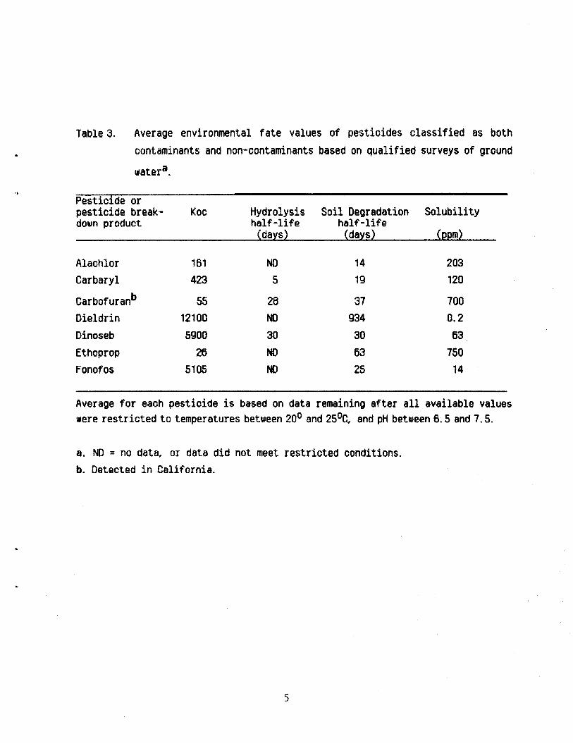
Table 3. Average environmental fate values of pesticides classified as both

contaminants and non-contaminants based on qualified surveys of ground

watera.

Pesticide or pesticide break- Koc Hydrolysis Soil Degradation Solubility down product half -life half-life

(days) (days) (Pm)

Alachlor 161 ND 14 203 Carbaryl 423 5 19 120

Carbofuranb 55 28 37 700 Dieldrin 12100 ND 934 0.2 Dinoseb 5900 30 30 63 Ethoprop 26 ND 63 750 Fonofos 5105 ND 25 14

Average for eaoh pesticide is based on data remaining after all available values were restricted to temperatures between 20' and 2S°C, and pH between 6.5 and 7.5.

a. ND = no data, or data did not meet restricted conditions. b. Detected in California.

detections. As a result, one study by the Iowa Department of Water, Air and Waste

Management is the only qualified reference for most of the pesticides appearing

in the non-contaminant group (Kelley and Wnuk, 1986).

In the initial categorization of pesticides into contaminant groups, azinphosmethyl, bromacil and terbufos were classified as contaminants, while

lindane and heptachlor were included in the transition category. After review of

the studies where these results were reported, azinphosmethyl, bromacil and

terbufos were removed from the contaminant group, and lindane and heptachlor were

moved into the non-contaminant group due to questions about the integrity of

sampled wells, the existence of extreme conditions, or suspect analytical

procedures (Appendix A).

Once a candidate list of contaminant and non-contaminant pesticides was developed

from the detection history summary, the corresponding environmental fate data

were extracted from the data base using a series of screening criteria.

Several screening criteria were applied to the environmental fate data during

extraction from the data base. Duplicate values given by several authors were

eliminated if cross referencing clearly occurred. Values were also restricted to

a pH range of 6.5 to 7.5, and to temperatures between 20” and 25°C on the

assumption that these represent general environmental conditions in California

agricultural soils. Whenever pH or temperature data were missing, it was

assumed that values fell within the acceptable range determined by the screening

criteria as unusual experimental conditions are frequently specified, when they

occur. Soil adsorption and soil degradation data were not restricted by soil

type, unless the values had been obtained using sterile soil or activated sludge.

Soil adsorption coefficients (Koc) were calculated from reported Kd values only

1 when the percent organic carbon content was known . No further calculation or

estimation of missing values was attempted. An average value for each

environmental fate variable was calculated after extraction from the database

.--_-----_------------------- 1. Koc =Kd / organic carbon fraction.

6

(Tables 1,2 and 3). Average values were then converted to logarithmic

equivalents both to normaliae the variable distributions, and to aid data

processing.

Statistlcalhnalyais Distributions of the transformed values for each variable in contaminant and

non-contaminant groups were tested for normality, and analysis of variance

(ANOVA) was conducted to determine if significant differences were present in Fhe

distribution of variables between contaminant and non-contaminant pesticide

groups. Then least significant difference (LSD) tests of each variable, as well

as standard deviations from group means and ninetieth percentile Intervals, were

calculated to determine potential specific numerical values. Transition

pesticides wh$ch had been reported as both contaminants and non-contaminants j.n

qualified studies were not included in the statistical analyses. ALI analyses

were performed using SAS@ software (SAS, 1978).

The LSD between means of two distributions, or treatments, is a type of t-test

based upon the combined standard errors of each treatment multiplied by a t value

refl’ecting a chosen level sf significance:

LSD = t,o5 tS12/rl f S22/,2), (Equation $1

where Sx2 = estimated variance of treatment x, x = number of observations In

treatment x, and t,O5 = tabular t value for degrees of. freedsm, (Little and Hill.,

1978,) When using the LSD test, contaminant (xc> and non-contaminant (xnc) group

means are considered to be significantly different if the absolute distance

between them $6 greater than the calculated LSD (Ix,-Xncf>LSD)+ The LSD can be

used as a measure of the maximum difference between the values of a group mean and

an independent qbservation, in order for the observation to be considered a

member af the group represented by the mean. The SNV for Koc was calculated by

subtracting the LSD from the mean of the contaminant group (SW = x,-LSD), The

SNVs for water solubility, hydrolysis half-lj.fe and soil degradation half-life

were calculated by adding the LSD to the positive group means (SNV = xc+LSR),

SNVs calculated in this manner represent the largest or smallest values that

statlstically fall withi.n the 95% confidence limit of the contaminant group mean.

7

Strictly speaking, SNVs should not be determined for hydrolysis or soil

degradation half life using this method, as the LSD test is invalid when there are

no significant differences between group means (Table 5).

Two other statistics of the environmental fate variable distributions were used

to calculate potential SNVs. The standard deviation and 90th percentile are

statistics whichmeasure the dispersion of normally distributed populations. One

standard deviation from the contaminant group means of water solubility and Koc,

and one standard deviation from the combined contaminant and non-contaminants

means of the hydrolysis half-life and soil degradation half-life distributions

were used to determine potential SNVs. Combined contaminant and non-contaminant

distribution of hydrolysis and soil degradation half life were used since there

were no significant differences between contaminant and non-contaminant groups

for these two variables according to the ANOVA (Table 5). Approximately 84% of

the contaminant pesticides have values exceeding an SNV determined by one

standard deviation from the contaminant or combined group means, based on the

normal probability distribution *. Similarly, SNVs based on the 90th percentile

of the contaminant or combined distributions represent values which

approximately 90% of the contaminant pesticides will exceed. SNVs based on the

90th percentile are slightly more conservative than SNVs based on one standard

deviation from the mean, because there is a higher probability that a pesticide

will exceed an SNV based on 90% of a normal distribution.

RESULTS

The values of the contaminant and non-contaminant group means, LSDs, standard

deviations and 90th percentiles used to calculate the numerical thresholds of

the environmental fate variables using transformed data are shown in Table 4.

SNVs calculated by the LSD method were least conservative, while SNVs based on

the 90th percentile were most conservative (Figures 1 and 2). Separate SNVs

could not be set for aerobic and anaerobic metabolism or field dissipation

because of insufficient data. For the present, the SNVs for these degradation

----- -- -.-- 2. In this discussion, values

- ---- - ------, 7”-- ----I-.. ?‘-^--- ---------. _-----_----u_ exceeding the proposed SNVs refer to wGyF

solubility, hydrolysis and soil degradation half-lives greater than the numerical value of the corresponding SNV. Koc values 'exceeding' the proposed SNV are less than the numerical value of the SNV.

8

Figure 1. Stylized distributions of log Koc and log solubility of contaminant (C) and non-contaminant (NC) pesticide groups based on group means and standard deviations.

SNV3

log Koc

SNVP

Cumulative portion of non-contaminant distribution exceeding SNVl

q Cumulative portion of hon-contaminant distribution exceeding SNV2

q Cumulative portion of non-contaminant distribution exceeding SNV3

SNVl: specific numerical value based on LSD. SNV2: specific numerical value based on standard deviation. SNV3: specific numerical value based on 90th percentile. xc : contaminant group mean. Xnc : non-contaminant group mean. LSD : least significant difference. S : standard deviation. 90% : 90th percentile.

9

Figure 2. Stylized distributions of log hydrolysis half-life and log soil degradation half-life of contaminant (-I-), non-contaminant (m-11) and combined (X) pesticide groups based on group means and standard deviations.

SNV3

SNVP I

c

log Hydrolysis

SNV3

SNVP

-1 0 1 2 3 4 5

90% I

% E”C I

q Proportion of combined contaminant and non-contaminant distributions exceeding SNV3

q Proportion of combined contaminant and non-contaminant distributions exceeding SW2

SNV2: specific numerical value based on standard deviation. SNV3: specific numerical value based on 90th percentile. xc : contaminant group mean. Xnc : non-contaminant group mean. X : combined contaminant and non-contaminant group mean. s : standard deviation. 90% : 90th percentile.

10

Table 4. Descriotive statistics of environmental fate variables of contaminant and non-contaminant pesticides used to calculate specific numerical values.

Environmental fate variables xnc Xnc,c LSD s 9O%tile

log Koc

log solubility 1.8403 2.3167 na (pm> (n=l9) (n-17)

log hydrolysis half -1if e (days)

log soil degradation half-life (days)

3.5740 2.1250 na (n=I6> (w14)

0.3306 0.5846a 2.8!Ma

0.5449 1.451P 0.2911a

na na 1.9233= (n=21) nsb

0.7988' 0.85;8c

na na 1.7446c (n=35) ns

b 0.7130' 0.9006c

na = not applicable to calculation of SNV's; Xno = non-contaminant mean; xc = contaminant mean; Xnc, c = combined contaminant and non-contaminant mean; s = standard deviation; 90ttile = 90th percentile.

a. statistic of contaminant group.

b. not significant (p>O.OS).

C. statistic of combined contaminant and non-contaminant groups.

11

lable 5. Analysis of variance (ANOVA) of contaminant, non-contaminant and transient pesticide groups.

log Koc 9.96 * 0.0004 34

log solubility (w-d

4.64 * 0.0154 40

log hydrolysis half-life (daysj

2.42 0.1173 18

log soil degradation half-life (days)

0.33 0.7239 32

Comparisons significant at the 0.05 level are indicated by I*'. Significant differences were between contaminant and non-contaminant groups only.

.

12

Table 6. Specific numerical values calculated using univariate statistical methods.

nethoo environnentala orooosedb nisclassifiedC nisclassifiedd fate v?riable SNU contaminants non-contaminants

least significant difference (LSD) fron contaninant nean

Koc uater solubility hydrolysis half-life soil degradation

half-life

1285 1 59 1 70

1 23

naled, (carbof uranj, oxamyl (ethoprop)

one standar ci deviation fron contaninant nean.

koc water solubility

one standard hydrolysis half -1if e deviation f ran soil degradation combined contaminant half-life and non-contaninant nean.

1 13

1 11

90th percentile of contaainzkt distribution.

Koc i785 water solubility 2 2

90th oercentile of conbined contatlinant and non-contaninant distribution.

hydrolysis half-life soil degradation

half-life

L 7

2 8

oxamyi dicamba, (alachlor j, (carbaryl j,

(carbof wan j, (ethcpropj

oxamyl dicamba, (alachlor), (carbarylj, (carbof uranj. (ethoprop)

Solubility in parts per million (ppm), hydrolysis half-life and soil degradation half life in days.

.

a. Soil degradation half-life includes aerobic and anaerobic metabolism, and field dissipation half-life.

b. SNV signifies 'specific numerical value'.

c. Pesticides from contaminant group not classified as contaminants using SNV's.

d. Pesticides from non-contaminant groups, transition pesticides(shown in parentheses), which were classified as contaminants using SNV's,

13

variables will be represented by the SNV for soil degradation half-life.

Specific numerical values calculated by eachmethod are shown in Table 6.

To be classified as a potential ground water contaminant according to the

Pesticide Contamination Prevention Act, a pesticide must exceed SNVs set for

either solubility or Koc, and either soil or hydrolysis half-life. Specific

numerical values were applied to average values of the contaminant,

non-contaminant and transition pesticide groups to evaluate the accuracy of

pesticide classification by each of the univariate methods. Two known

contaminants, naled and oxamyl (Table 11, were not classified as contaminants

using SNVs calculated from the LSD test, and only two of the possible seven

contaminants in the transition group (Table 3) were classified as contaminants

using the same SNVs. Application of the SNVs calculated using the standard

deviation of variable distribution classified all known contaminants except \ oxamyl as contaminants, and classified a substantial portion of the transition

pesticides as contaminants (Table 6). One non-contaminant pesticide, dicamba,

was classified as a contaminant. Classification of pesticides using SNVs based

on the 90th percentile were not different from the classification obtained using

SNVs based on one standard deviation. Considering their relative performance,

the SNVs calculated using one standard deviation of envlronmental fate

distributions are acceptable indicators of potential contaminants and are more

conservative than criteria for environmental fate variables proposed by the US

EPA (Creeger, 1986).

DISCUSSION Methods other than univariate statistics were considered for determining SNVs,

including simple transport models and multivariate statistical analyses. Each of

the methods present different advantages and disadvantages to pesticide

classification.

The univariate methods for setting specific numerical values were based on two

critical assumptions. First, we assumed that pesticides may be classified

correctly as contaminants or non-contaminants based on historical monitoring

data. Several problems are involved with this assumption: incidences of

contamination were reported from widely different geographical sett-lnqs

throughout the United States, and most individual monitoring efforts were

14

relatively limited in the number of pesticides sampled and in the spatial extent

of well sampling. Therefore , pesticides which were classified as contaminants

because they were detected in one location may not be contaminants in less

vulnerable agricultural settings when appropriate use practices are followed.

Conversely, the classification of a pesticide as a non-contaminant does not ’

preclude the possibility that it will move through soil to ground water depths

under extreme environmental conditions, or that it does not already occur in

ground waters which have not been surveyed. The classification of pesticides

into contaminant and non-contaminant groups is perhaps the most critical step in

setting SNVs by any statistical method. Changes in the classification of

pesticides from non-contaminant to contaminant based on future surveys, or the

addition of new pesticides to these groups, will probably require the revision of

the SNVs proposed here.

The second assumption for setting SNVs concerns the treatment of data collected

for each pesticide.. We assumed that average values of solubility, Koc,

hydrolysis and soil degradation half-life adequately represent the

characteristic properties of pesticides, despite the enormous amount of

variability that is frequently reported for these variables; values ranging over

one or two orders of magnitude are not uncommon, even when measurements are made

under controlled conditions. We did not attempt to identify single ‘best’ values

to represent the environmental fate characteristics of each pesticide from the

data that were available, but accepted all values falling within a limited range

of, temperature (20”“25°C) and pH (6.5-7.5). In fact, there are no standard

conditions or standard media established for the measurement of the

environmentally sensitive variables: Koc, hydrolysis half-life and soil

d,egradat5on half-llf e. The decision to calculate SNVs with data obtained under

the two assumptions discussed above was based on the belief that the amount of

va.riation ‘built-in’ to average environmental fate values obtained from

different experimental conditions complements the uncertainty in the

classification of pesticides as contaminants or non-contamPnants, resulting in

the broadest possible description of relatl.ve pesticide behavior in the

envi ronmen t .

Multivariate statistical analysis. is another approach that could be used to

Identify potential contaminant pesticides. A multivariate treatment such as

principal components analysis would identify combinations of variables that

15

.

could be tested for their predictive capability. Like univariate analysis,

multivariate combinations of environmental fate variables would not presume the

quantitative relationship of variables theoretically involved in pesticide

transport, or the conditions of pesticide use and geographical setting. In this

type of analysis, additional environmental fate and chemical properties could be

included to more fully describe pesticide chemistry and establish classes of

pesticides. For example, physico-chemical properties such as vapor pressure,

molecular mass, boiling point, melting point and others could be included in the

statistical analysis. A multivariate combination of many chemical properties

would lessen the overriding influence of any one property on the predicted

result, increasing the flexibility and accuracy of the statistical model. A

multivariate analysis may require more data, but this disadvantage would be

partially offset by the use of basic chemical measurements which are more

generally available and standardized. The application of this method would also

require a departure from the screening mechanism currently prescribed by Section

13144(b)[2] of the PCPA.

Several mathematical screening models which simulate pesticide transport through

soil have been formulated in recent years (Jury, et al, 1984, Enfield, 1985,

Carsel et al, 1985). These models are usually based on variations of the

advection-dispersion equation, and assume linear, reversible and instantaneous

equilibrium adsorption and first order degradation rates of pesticides moving

through uniform soil matrices. Within a given soil matrix, pesticide velocity in

solution is calculated as a function of the soil adsorption coefficient (Koc).

Pesticide concentration over time is a function of the quantity of pesticide

initially available to the system, minus the quantity lost through degradation

processes. Thus, the models attempt to estimate both the time required for a

pesticide to arrive at a certain point in the soil profile, and the concentration

expected at the time of arrival. The relative mobility and persistence of

pesticides may be ranked within a given soil matrix by comparing their

environmental fate properties (Koc and soil degradation). Screening models

facilitate the comparison of pesticide transport through different soil matrices

by altering the values of bulk density, organic carbon content and volumetric

water content and water flux, allowing changes in velocity of a pesticide through

the soil to be related to different environmental conditions. While there are

some apparent advantages in using screening models to identify potential ground

water contaminants, there are also some significant drawbacks.

16

The use of a screening model to set SNVs based on theoretical equations governing

solute transport, is appealing because this approach appears to include the

ef feet of different environmental settings, and considers quantitative

relationships between chemical and soil properties rather than arbitrary,

independent threshold values established by statistical comparison, However,

several underlying assumptions on which transport models are based have come

under increasing scrutiny. More importantly, the predicted behavior of large

numbers of pesticides have not been verified by field observation. Increasingly,

field observation of pesticide mobility indicates that transport models may

underestimate pollutant velocities by as much as 60 percent (Bowman and Rice,

1986 and Rice et al, 1986). Accelerated movement through preferential flow

pathways , changes in adsorption kinetics and other interactions between

environmental fate properties and physical soil properties have been implicated

as possible mechanisms to account for the discrepancy between field observation

and predicted behavior, but as yet these processes have not been sufficiently

described or incorporated into models of pesticide behavior.

CONCLUSION A univariate statistical procedure based on the comparison of designated

contaminant and non-contaminant pesticides was used to determine specific

numerical values (SNVs) for four environmental fate variables in accordance with

Section 13144 of the Pesticide Contamination Prevention Act. Comparison of the

environmental fate data of known contaminant and non-contaminant pesticides

indicated that pesticides with soil adsorption coefficient (Koc) values less than

512 cm3/gm or water solubility greater than 7 ppm, and hydrolysis half-life

greater than 13 days or soil degradation half-life greater than 11 days, may be

classified as potential ground water contaminants. The calculation of SNVs using

univariate statistics, and the mechanism for applying the SNVs as set forth in AR

2021, implies that single values of environmental fate variables exist which

would identify potential ground water contaminants, and that these ‘threshold’

values are successful’ regardless of the conditions of pestictde use or

geographical setting. The method on which the present calculationof SNVs was

based offers an advantage over other contaminant screening methods because it

uses environmental fate data in a manner that is quantitative, reproducible and

verifiable by historical detection data while adhering to a strict interpretation

of the requirements of Section 13144.

17

While the proposed SNVs satisfactorily classify certain pesticides as

contaminants or non-contaminants based on available data, other methods of

identifying potential contaminants may be developed which make more

comprehensive uses of pesticide characteristics and specific environmental

conditions. In this case, it is recommended that the implementation of Section

13144 be expanded to allow pesticide classification using a series of threshold

values, or mathematical equations.

. Environmental fate data for many of the pesticides used in the analysis were not

available, or did not meet specific criteria restricting data to a range of

standard conditions. For this reason, the proposed SNVs should be revised after

standardized environmental fate data are submitted to the Department of Food and

Agriculture as required by the data call-in portion (Section 13143) of the PCPA.

SNVs based on comparative statistical methods may also require revision as new

pesticide detections occur in ground water.

18

REFERENCES

Bowman, R.S. and R.C. Rice. 1986. Transport of Conservative Tracers in the Field Under Intermittent Flood Irrigation. Water Resources Research 22(11):1531-1536.

Brodies, J.E., W.S. Hicks, G.N. Richards, F.G. Thomas. 1984. Residues Related to Agricultural Chemicals in the Groundwaters of the Burdekin River Delta, North Queensland. Environmental Pollution (Series B) 8:187-215.

Bushway, R.J., W. Litten, K. Porter, and J. Wertam. 1982. A Survey of Azinphoa Methyl and Azinphos Methyl Oxon in Water and Blueberry Samples from Hancock and Washington Counties of Maine. Bulletin of Environmental Contamination Toxicology 29:354-359.

California Department of Food and Agriculture - unpublished report. Environmental Monitoring and Pest Management, 1985.

California Department of Food and Agriculture - unpublished report. Environmental Monitoring and Pest Management, Glenn County, 1985-1986.

Cardozo, C.L., S. Nicosia, and J. Troiano. 1985. Agricultural PesticideResidues in California Well Water: Development and Summary of a Well Inventory Data Base for Non-Point Sources. California Department of Food and Agriculture.

Carsel, R.F., L.A. Mulkey, M.N. Lorber and L.B. Baskin. 1985. Monitoring Ground Water for Pesticides in the USA- preprint. EPAOffice of Pesticide Programs.

Creeger, Samuel M. 1986. ‘Considering Pesticide Potential for Reaching Ground Water Registration of Pesticides’ in: Evaluation of Pesticides in Ground Water, ACS Symposium Series 315, W.Y. Garner, R.C.Honeycutt and H.N. Nigg, eds.

Enfield, C.G. 1985. Chemical Transport facilitated by multiphase flow systems. Water Sci Tech 17:1-12.

Exner, M.E. and R.F. Spalding. 1985. Ground Water Contamination and Well Construction in Southeast Nebraska. Ground Water 23(1):26-34.

Frank, R., B.0, Ripley and G.S. Sirons. 1979. Herbicide Contamination and Decontamination of Well Water in Ontario, Canada, 1969-78. Pesticide Monitoring Journal 13(3):120-127.

Greenberg, M., R. Anderson, J, Keene, A. Kennedy, and S. Schowgurow, 1982, Empirical Test of the Association Between Gross Contamination of Wells with Toxic Substances and Surrounding Land Use. Environmental Science of Technology 16(1):14-19.

Harkin, J.M., E.K. Dzantor, R. Fathulla, F.A. Jones, E.J. O’Nei.11, et al, 1984. Pesticides in Groundwater Beneath the Central Sand Plain of Wisconsin, University of Wisconsin, Water Resources Center, Project No. A-094-WIS.

Jury, W.A., W.F. Spencer and W.J. Farmer. 1984. Behavior assessment model for tracer organics in soil IV. AppliCatiOn of screening model. J. Environ. Qual, 13:573-579.

19

Katz, G.B. and G.E. Mallard. Chemicals and Microbiological Monitoring of a Sole-Source Aquifer Intended for Artificial Recharge, Nassau County, New York.

Kelley, R. and M. Wnuk. 1986. Little Sioux River Synthetic Organic Compound Municipal Well Sampling Survey. Iowa Department of Water, Air and Waste Management.

LaFleur, K.S. 1976. Movement of Carbaryl Through Congaree Soil Into Ground Water. Journal of Environmental Quality 5(1):91-92.

Little, T.M. and F.J. Hill. 1979. Agricultural Experimentation: Design and Analysis. John Wiley and Sons, New York.

Maddy, K.T., D.W. Conrad, H.R. Fong, A.S. Fredickson and J.A. Lowe. 1982. A Study of Well Water in Selected California Communities for Residues with 1,3-Dichloropropene, Chloroallyl Alcohol and 40 Organophosphate or Chlorinated Hydrocarbon Pesticides. Bulletin Environmental Contamination Toxicology 29:354-359.

Marti, L.R., R.C. Dougherty, and J.R. Kanel. 1984. Screening for Organic Contamination of Groundwater: Ethylene Dibromide in Georgia Irrigation Wells. Environmental Science of Technology 18:873-874.

Peoples, S.A., C. Cooper, W. Cusick, A.S. Fredickson, T. Jackson and K.T. Maddy. 1980. A Study of Samples of Well Water Collected from Selected Areas in California to Determine the Presence of DBCP and Certain other Pesticide Residues. Bulletin of Environmental Contamination Toxicology 24:611-618.

Rice, R.C., R.S. Bowman and O.B. Jaynes. 1986. Precolation of Water Below an Irrigated Field. Soil Sci Am. J. 50:855-859.

SAS: Statistical Analysis System. 1979 SAS Institute Inc., Box 8000, Cary, North Carolina 27511, USA.

SIR': Scientific Information Retrieval, Inc. 707 Lake Look Road, Deerfield, IL 60015, USA.

Spalding, R.F., G.A. Junk, and J.J. Richard. 1980. Pesticides in Ground Water Beneath Irrigated Farmland in Nebraska, August 1978. Pesticide Montioring Journal 14(2):70-73.

STORET: Gross Inventory of Groundwater Monitoring Results from 3/l/84 to 6186.

Wehtje, G., J.R.C. Leavitt, L.N. Mielke, R.F. Spalding and J.S. Schepers. 1981. Atrazine Contamination of Groundwater in the Platte Valley of Nebraska from Non-Point Sources. The Science of the Total Environment 21:47-51.

Zaki, M.H., D. Harris, and D. Moran. 1982. Pesticides in Groundwater: The Aldicarb Story in Suffolk County, New York. American Journal oE Public Health 72(12):1391-1395.

20

APPENDIX A

21

UNIVERSITY OF CALIFORNIA, RIVERSIDE

BERKELEY - DAVIS . IRVISE * LOS ANGELES * RIVERSIDE * SAN DIEGO - SAN FMh‘CISCO SAhTh BARBARA ’ SANTA CRUZ

COLLEGE OF NATURAL AND AGRICULTURAL SCIENCES RIVERSIDE, CALIFORNIA 92521.0424

CITRUS RESEARCH CENTER AND A~RI~~LT~RALEXPERIMENT STATION

DEPARTMENT OF SOIL AND ENVlRONhlENTAL SCIENCES January 7, 1987

Ms. Muffet Wilkerson Environmental Monitoring, Room A-149 Department of Food and Agriculture 1220 "N" Street Sacramento, CA 95814

Dear Muffet:

I have reviewed the draft copy of your report entitled i%e Pesticide Groundwater Prevention Act: Setting Specific Numerical Yalues which I received on approximately X.11-86.

The use of a statistical approach as you describe in your report to establish the specific numerical values for pesticides is understandable given the framework of the regulation and the need to provide a quantifiable and varifiable method. Rowever, I fully support your recommendation that additional procedures including the use of mathematical models for predicting pollution potential of groundwater be pursued. As an example of one of the benefits to be derived, the use of such a model would allow combinations of environmental factors to be used to predict pollution potential rather than relying on a specific numerical value. For example, as the property of soil adsorption coefficient decreases, and a compound becomes more mobile in soil, compounds of shorter half-life would be more likely to reach groundwater. On the other hand, compounds with high soil adsorption would require a longer half-life in order to reach groundwater. Such combinations of two properties whose values vary depending on each other cannot be easily attained with single specific numerical values.

As we have discussed in the past, there are several advantages and disadvantages to the use of the statistical approach many of which you have presented. One of the advantages of the

22

statistical approach is that it allows a testing of previous investigations into the factors controlling the movement of pesticides in soil. Presumably the pesticide properties of soil adsorption coefficient , water solubility, hydrolysis, aerobic and anaerobic soil metabolism, and field dissipation became a part of the present regulation because of the extensive evidence existing in the pesticide literature based on laboratory and field studies and on mathematical modelling which showed these properties as prime indicators of the leaching potential of a pesticide. Now that pesticides are being detected in the groundwaters of this state and of the country, it is possible to apply statistical approaches such as you have used to evaluate these properties and determine if there is a relation between the specific numerical values of these pesticide properties and the detection of pesticides in groundwater, As you pursue your investigation of predictive models, perhaps more of these relationships will become evident.

One of the unavoidable disadvantages of the use of a statistical approach at this time is the lack of sufficient data. This lack is evident both in the number of pesticides present in both the contaminant and noncontaminant groups and in the lack of environmental fate data for the pesticides. As monitoring for pesticides in groundwater continues, the data base will doubtlessly increase thereby improving the potential usefulness of the statistical approach. In this regard, it is my opinion that the list you show in your report as the transient group should be included in the contaminant list. Currently there is a tendency for investigators to report only positive but not negative results in groundwater monitoring. As the reporting of negative results becomes more common place, I think many of the compounds on the contaminant list would be shifted to the transient group using the present criteria.

The lack of environmental fate data for the individual compounds is the most serious drawback to the present use of the statistical approach. As you state, this situation will improve 3s the data call in phase of this regulation begins. However,

23

there will always be uncertainties in the data such as in soil adsorption and field dissipation rates due to influences of such variables as soil type, temperature, and moisture.

One of the possible results of the lack of sufficient data is what appears to be the low value you report for the specific numerical values. These values are considerably more conservative than the values suggested by EPA and could result in a large number of compounds targeted as potential groundwater contaminants. As the data base improves, this may change. That is, when the list of compounds is small as it now is, a few pesticides with unusual properties can have a large influence on the final outcome. As the number of pesticides and pesticide properties in the set increases, the result should become more representative.

The use of the soil degradation half-life value for aldicarb shown in Table 1 would contribute to a low specific numerical value for this property. The aldicarb value is probably not representative of the groundwater pollution problems that have been associated with the use of this compound. It would be better to use the half-life value for the toxic degradation products of aldicarb. It is usually the total toxic residues for a pesticide that are reported in groundwater. For aldicarb this would include aldicarb and its toxic degradation products, the sulfoxide and sulfone.

The lack of any significant differences between the means of the contaminant and noncontaminant groups for the properties of hydrolysis and soil degradation is noteworthy and doubtlessly illustrative of the lack of sufficient data points. Soil degradation is known to be a significant factor influencing the potential for movement in soil.

The use of a depth variable soil degradation rate may prove to be a significant improvement in assessing movement to groundwater. Field dissipation rates for pesticides generally decrease with soil depth due to a number of factors such as reduced

24

volatilization to the atmosphere, reduced photodecomposition, reduced aeration and a significant reduction in the number of soil microorganisms. Data on the variation in the rate of degradation with soil depth is beginning to accumulate in the literature and should prove useful in future evaluations of the specific numerical values.

Sincerely,

Walt&r J. Farmer Professor of Soil

Chemistry

WJF:mds

cc: J. N. Seiber W. F. Spencer W. A. Jury

25

.

UNIVERSITY OF CALIFORNIA, DAVIS .,...... “.

BaE,.EY l DAVIS - IR\‘ISE * LOS ANGELES * RIVERSIDE ’ SAN DIEGO ’ SAN FRANCISCO SAhTA BARBARA l SAlTA CRUZ

COLLEGE OF AGRICULTURAL AND ESVIRONMESTAL SCIENCES AGRICULTURAL EXPERIMEST STATION (916) 752-l 142

DEPARTMENT OF ESVIRONMENTAL TOXlCOLOGY DAVIS. CALIFORNIA 95616

December 2, 1986

Ms. Muffet Wilkerson Environmental Monitoring, Rom A-149 Department of Food and Agriculture 1220 "N" Street Sacramento, CA 95814

Dear Muffet:

I read over your draft of November 6, 1986, on "Setting Specific Numerical Values."

In Table 1 and 2, 1 question the water solubility of naled (0.33 ppm) which seems low even considering the 2 bromine atoms. Also question for aldicarb whether entries should be made for sulfoxide and sulfone, because these are usually the products found in groundwater. Units should be specified for the last 3 columns. We have to keep an eye on the soil degradation half lives because if they are determined from field data the more volatile surface applied chemicals such as toxaphene (and perhaps oxamyl) will show relatively short half-lives, because of volatilization, where in fact they could have very long half-lives if volatilization were not pronounced. Similarily, aldicarb soil half-life (7 days) may be for the parent rather than the sulfoxide/sulfone.

In Table 5, you calculated an average only, without a confidence interval. Perhaps the averages should be given as e.g. Koc = < 360 f 50 (95% confidence), and thus Koc in Table 6 would be set at 310 to reflect the lower (more conservative) range of Koc. (I estimated the 250 -- needs to be calculated accurately.) If you did it that way, diuron would then become a 'potential yes' although you would still miss on oxamyl.

The oxamyl case is interesting, because it tends to argue in favor of the Jury-Focht-Farmer approach for considering an interaction between numerical values. Oxamyls exceptionally high water solubility can apparently compensate for its low half-lives in soil and water, particularly when applied to a porous soil under high moisture penetration conditions (and coupled with groundwater analysis taking place relatively soon after application! 1.

I question the finding of carbaryl in groundwater. The LaFluer reference used W spectrophotometry at 222 nm to detect carbaryl. This is a very non- specific method, and even the authors themselves admitted that l-naphthol and methyl isocyanate (degradation products of carbaryl) could have contributed to

26

the absorbance. (In fact, all of the absorbance could have been due to naphthol! ). Although they did not specify their detection limit, it probably was 0.1 PMole/liter (the lowest 'positive ' finding) and the maximum observed was 0.3 PMole/liter. Not very convincing1 In my opinion, this report should not be given much weight.

Ethoprop, from its structure and properties, looks like a good candidate for groundwater contamination. I believe that it is also used as a soil nematicide. Thus, I was pleased to see that you predicted positive for it. The negative finding by Marti et al., which is based on very convincing anlaytical data, may be due to the depth of the wells (150 ft) which penetrated the Ocala limestone aquifer. I could not find any information in this article on the soil type or depth to groundwater. Thus, I feel ethoprop does indeed carry potential, at least for shallow wells under sandy soils.

I would be pleased to review any of the references an analytical finding (positive or negative) if you point me in the right direction.

Best regards, n

JNS:gm cc: Walt Farmer

27

J&es N. Seiber Professor

UNIVERSITY OF CALIFORNIA, DAVIS . ..“....~

BERKELEY l DAVIS. RWINE - LOS ANGELES *RIVERSIDE l SAN DIEGO l SAN FFtA?XISCO SAN-l-A BARBARA l SANTA CRVZ

COLLEGE OF AGRICULTURAL AND ENVIRONMENTAL SCIENCES DEPARTMENT OF EKVIRQKMENTAL TOXICOLOGY

AGRICULTURAL EXPERIMENT STATION DAVIS, CALIFORSIA 95616

(916) 752-l 142

October 6, 1986

Ms. Muffet Wilkerson Environmental Monitoring Room A-149 California Department of Food and Agriculture 1220 N Street Sacramento, CA 95814

Dear Muffet:

Following are my observations dn the reported finding of azinphosmethyl in a well located within a treated blueberry field [Bull. Environ. Contamin. Toxicol. 28. 341 (198211.

1.

2.

A . -

Azinphosmethyl was determined to be present in samples collected 7/9 (1.9 ppb), 7/14 (11.2 ppb), 7/23 (24 ppb) from a single well.

Azinphosmethyl was not detected (i.e. < 0.23 ppb) on 8/11 in a sample(s) from the same well.

3.

4.

5.

6.

The type of well was not described, except that it was a household well, nor was its configuration in the treated field or its depth presented.

No information on the number of samples, or standard deviation of replicates, was given.

No azinphosmethyl was found in surface runoff from any fields in the study.

The fields are described as glaciomarine deltas--gravel and sand.

I don't believe that this study should be given much weight as indicative of a tendency of azinphosmethyl to move into groundwater. If the positive well samples were the result of azinphosmethyl leaching through the "soil", it is surprising that the levels would have declined so dramatically from the 7/23 to 8/11 samples, because pesticides rarely leach through soil as a quick- moving, quick-clearing plug of material. If azinphosmethyl did behave this way, it seems likely it would have been found in surface water runoff, too.

I think that the results are consistent with direct introduction of material to the well water during application and subsequently by rain washing more material from the well covering into the well.

28

Even if the well contamination were due to leaching, the unusual soil characteristics (sand and gravel) preclude any generalizations.

Unless this finding is corroborated by other investigators in other locations, I do not believe that this study should be included in defining those pesticides found in groundwater in connection with the AB 2021 data call-in.

Best regards,

JNS:jls

29