the performance of the billing process at hi3g access ab · of the billing process at hi3g access...
TRANSCRIPT

The Performance of the Billing Process
at Hi3G Access AB
H O M I N G W U
Master of Science Thesis Stockholm, Sweden 2008

The Performance of the Billing Process
at Hi3G Access AB
H O M I N G W U
Master’s Thesis in Computer Science (30 ECTS credits) at the School of Computer Science and Engineering Royal Institute of Technology year 2008 Supervisor at CSC was Inge Frick Examiner was Karl Meinke TRITA-CSC-E 2008:046 ISRN-KTH/CSC/E--08/046--SE ISSN-1653-5715 Royal Institute of Technology School of Computer Science and Communication KTH CSC SE-100 44 Stockholm, Sweden URL: www.csc.kth.se

Abstract
The performance of the billing process at Hi3G Access AB
Hi3G Access AB in Sweden has customers both there and in Denmark. Every month the billing process needs to calculate the invoices for the customers and this process takes a long time to complete. The purpose of this master Thesis project was to investigate the performance of the billing process at the company and search for ways to improve it. This report will show the methods used and discoveries found during the project. The result chapter at the end of the report describes that the overall performance gain was largest with a server configuration setup. Optimizing the software in the system such as functions used in the billing process gave minor performance benefits. The server configuration results are incomparable with the function optimization’s results, because the numbers of investigated functions where to few to draw any conclusions.
Sammanfattning
Faktureringsprocessens prestanda hos Hi3G Access AB
Hi3G Access AB i Sverige har både kunder här och i Danmark. Varje månad beräknar faktureringsprocessen kundernas fakturor och denna process tar lång tid att utföra. Examensarbetet undersöker prestandan på faktureringsprocessen samt hittar lösningar för att förbättra den. I rapporten beskrivs arbetsgången och metoderna som användes i projektet. Resultatet är att prestandavinsten var störst med server-konfigurationer. Att optimera mjukvaran i systemet som i form av utförda funktioner gav en mindre prestandavinst jämfört med serverkonfigurationen. Mängden av undersökta funktioner var inte tillräcklig för att avgöra om dessa funktionsoptimeringar kan ge en större prestandahöjning.

Acknowledgment
First I would like to thank my supervisor Mattias Nilsson, Malin Sjöblom and the manager of Human Resource Jessica Joelsson for choosing me to do the Thesis project at 3. Many thanks to Paul Velenik as my project supervisor for your guidance and your patient for every time you sat down and explained how things work is really appreciated. I also want to thank everyone at 3 that helped me with this project especially Henrik Gillingstam at the Oracle group for helping me with database questions, and a special thanks to Adam Tong for his expertise in Singl.eView. Last I want to thank my supervisor Inge Frick at KTH that helped me with the report. Last but not least thanks for all the ‘fikas’ from the Billing team, it has been fun.

List of Abbreviations
BGP Bill Generation Process CCP Customer Child Processes DB2 Denmark Business 2 DC4 Denmark Consumer 4 ECP Event Child Processes ENM Event Normalization Process EPM Expression Parser Module ERT Event Rating Process GUI Graphical User Interface IGP Invoice Generation Process IMSI International Mobile Subscriber Identity I/O Input / Output MSISDN Mobile Subscriber Integrated Services Digital Network Number NCP Node Child Processes NODB Non database server RAID Redundant Array of Independent Disks RGP Rental Generation Process RODB Read only database RWDB Read and write database SAN Storage Area Network SB3 Sweden Business 3 SC6 Sweden Consumer 6 SCP Service Child Processes SQL Structure Query Language SSH Secure Shell

Table of Contents
1 Introduction ............................................................................................................................. 1
2 Description of the system ........................................................................................................ 1
2.1 The Rental Generation Process ................................................................................... 3
2.2 The Bill Generation Process ........................................................................................ 4
2.3 The Image Generation Process .................................................................................... 4
2.4 A Bill Cycle ................................................................................................................. 5
2.5 Streams ........................................................................................................................ 6
3 Theoretical background ........................................................................................................... 7
3.1 Parameter explanation for the Excel tool .................................................................. 10
4 Methods ................................................................................................................................. 12
4.1 Method R ................................................................................................................... 13
4.2 Applying methods ..................................................................................................... 14
5 The Project’s Work Process .................................................................................................. 14
5.1 Preparations ............................................................................................................... 14
5.2 Server Configuration Overview ................................................................................ 16
5.3 Performed Configuration Tests ................................................................................. 20
5.3.1 Performance Tests Part One .............................................................................. 20
5.3.2 Performance Test Part Two ............................................................................... 21
5.3.3 Performance Test Part Three ............................................................................. 25
5.4 Function analysis ....................................................................................................... 28
5.5 Top functions ............................................................................................................. 28
5.6 Function test .............................................................................................................. 30
5.7 Statspack .................................................................................................................... 32
6 Performance tests’ results ...................................................................................................... 35
6.1 Part one: Performance tests’ with around 5000 customers ........................................ 36
6.1.1 Summary for Part One ....................................................................................... 41

6.2 Part two: Results from the 100 customers cycles ...................................................... 42
6.2.1 Summary for part two ........................................................................................ 43
6.3 Part three: Results from the 2000 customers cycles .................................................. 47
6.3.1 Summary for Part three ...................................................................................... 48
7 Conclusion ............................................................................................................................. 52
8 Future development ............................................................................................................... 53
8.1 How to approach the production machine ................................................................. 55
8.2 Possible problems during a bill-run ........................................................................... 56
9 Discussion ............................................................................................................................. 58
Reference.......................................................................................................................................... 60
Appendix A ...................................................................................................................................... 61
Tools ...................................................................................................................................... 61
Appendix B ...................................................................................................................................... 62
Embedded excel spread sheet data ........................................................................................ 76
Appendix C ...................................................................................................................................... 86
Files ....................................................................................................................................... 86
Code ...................................................................................................................................... 86
Appendix D ...................................................................................................................................... 89
RAID description .................................................................................................................. 89
1
Introduction
1 Introduction
Hi3G Access AB1 also known as 3 is a telecom company that specializes in 3G and wireless broadband in nine countries all around the world. The billing department of the company is in charge of the system maintenance of the billing software. The software controls the logic behind the billing process and calculates the bills for the customers. A billing process at the company takes several hours to finish and the desire to improve the performance was raised. The goal of the Thesis project was to identify where in the billing process time was consumed and thus where changes could provide a significant performance improvement. Optimizing it will make the billing software more efficient in completing its task e.g. faster calculations of invoices. The project was structured thus:
• Analyzing the billing process in detail.
• Documenting all the information about where the billing process was most time consuming, this would make it easier for future optimizations.
• Suggesting solutions and implementing as many of these feasible solutions as possible and make a comparison on the performance after the changes have been applied.
2 Description of the system
The performance tests were conducted on two machines. The first machine was a Hi3G test environment server. It has eight 650 MHz processors inside and runs with a UNIX operating system called HP-UX 11i v1. The system has two internal hard drives with a capacity of 73 GB each and 50 connected SAN hard drives. SAN hard drives are discs that are linked through a network. The internal disks are configured with RAID 1 and the others are configured with RAID 5 with a total disk space of 4.1 TB (4100GB), see Appendix D about RAID [7]. Total physical RAM is 16GB.
The second machine was the development machine. It has four CPUs installed and each CPU has a clock frequency of 550 MHZ. The machine has two RAID 1 hard drives with disc space of 36.4 GB each. It has also five additional SAN discs with different size. The server has 6.1 GB of physical memory and uses the same UNIX version as the test machine.
The company uses a GUI (graphical user interface) program called Singl.eView. The program is used together with the backend (UNIX shell) for configuring Tuxedo processes that executes EPM (Expression Parser Module) code and starts different kinds of perl, shell scripts and other types of executables. EPM is a proprietary scripting language, which looks similar to C and Perl code. Below are a couple of details regarding the EPM scripting language:
• EPM supports both dynamic- and hard-types i.e. a variable can only support e.g. an integer and variables that can store an arbitrary data type.
1 For more information visit URL: http://www.tre.se, 2007

2
Description of the system
• EPM supports both variable passing by value, constant reference or reference.
• EPM supports a deterministic function parsing, which allows the function to parse once and be replaced by a constant if possible.
Tuxedo2 processes are the support processes’ that pass information from one process to another in a bill-run. They offer different services, for example: rental generation, bill generation, image generation etc. The rental generation calculates the fixed monthly cost that a customer has. The bill generation summarizes the total bill for a customer, while invoice generation creates a file that a printing company uses for printing and delivering the bills to the customers. To operate the remote servers the SSH client Putty3 for Windows platform was used. Through Putty we can access the UNIX system and issue commands that monitor and control the Tuxedo servers. For example manually stopping and restarting the Tuxedo processes or executing scripts. All the data that the Tuxedo processes create are stored in an Oracle database version 9.2.0.6.0.
Customers
Picture 2-1: Registering customers in the billing system
When a customer signs a subscription the information is stored in the billing system. When a customer reaches the billing period the system will automatically generate the monthly fees and calculate all the usage of a service during that period of time e.g. phone calls. Picture 2-2 shows the simplified version of the main steps involved in creating an invoice.
Picture 2-2: A simplified illustration of the billing process (bill-run)
Each month, a customer’s invoice is triggered by the billing system. When the system is executing the billing process it will check the database information related to the customer and run from the RGP process (Rental Generation Process) to the last step invoice.
The bill-run processes have three important steps: the Rental Generation Process (RGP), the Bill
Generation Process (BGP) and the Invoice Generation Process (IGP). There are a few more steps involved in a bill-run process, but those steps are not as time consuming as the major ones and require no further tuning for performance purposes and are not a part of this investigation. The most time consuming phases are the BGP and the IGP steps. These steps take 80 - 90% of the total time spent. 2 Tuxedo is a product from BEA www.bea.com
3 For more information see Appendix A under Tools.
RGP BGP IGP Invoice
The Billing System

3
Description of the system
2.1 The Rental Generation Process
This step calculates all the fixed subscription fees for customers and can be specified to run with a set of chosen customers in the RGP step and generate the fees used in the next BGP stage. Each calculation needs to fetch a “service”, “product”, “customer” and “tariff”. It may also find a “facility group” (not used at Hi3G Access AB but supported by Singl.eView) in order to know the correct type of fee (Intec pages 1.17-1.19) [4]. The service is the MSISDN IMSI pair (a unique id for a phone number) towards which the usage for a specific customer is guided and charged. The terminology for guiding can be described with a customer A and a customer B. When A wants to call B the system needs to match the IMSI pair number with the caller, but a phone number does not always have to have the same IMSI number e.g. when a customer joins a new operator the IMSI number will be changed while the phone number is still the same. When A calls B with her new IMSI number she will be guided to the correct operator and charged. The type of usage may be e.g. data traffic, a phone call or as in the RGP a recurring charge. Several products builds up a price plan i.e. a subscription sold to a customer. Products are also used to model campaigns (e.g. send SMSs for free at Christmas Eve) and add-on subscriptions that support charging e.g. downloading music. Tariffs in billing are the rules for a specific event and service to know how to set the prices or what price plan to choose from. Commonly different tariffs are used for the charge of different types of events e.g. one tariff is used to charge for content events and another tariff for recurring charges and so forth. There are also special tariffs triggered during the BGP steps that are not related to usage, such as to set a special condition e.g. 10% discount for all usage above a certain limit of usage. The next level of discount could be 30% when the usage reaches another higher limit or e.g. to support a max amount of invoices for corporate customers so that e.g. if one of the employees consume more than 500 SEK, then the invoice amount exceeding 500 SEK is sent to the employee and the company pays for the base cost of 500 SEK. In picture 2-3 we describe the RGP process in detail.
Get the information from database
Receive information
Picture 2-3: Description of the RGP process Intec [5]
DB
Calculate the period for each recurring tariff
Startup
Build a timeline
Generate rental events for each segments of the timeline
Store the information from previous step in a subsequence called Rental Adjustment Process
Send the information as events to ENM

4
Description of the system
What is ENM?
The Event Normalization Process (ENM) typically performs normalization of usage e.g. which number was dialed and who should be charged and so forth and converts events into normalized events (Intec page 1.12-1.15) [6]. The normalized event is a common data storage format that is used by other processes in the system.
2.2 The Bill Generation Process
During the BGP step the process summarizes all the usage in a detail specification for the customer, e.g. the number of sent SMSs or phone calls made during a valid billable period (Intec page 1.19) [5]. The calculation of discounts or other special offers e.g. discounts such as 10% on the invoice amount or similar that will change the total price for the customer will also be calculated. All these calculations are stored in a database table called Charge. This step usually takes approximately 40 - 50% of the total processing time for a bill-run. The number was taken from the bill-run statistics, see picture 6-5 to 6-7. This is together with the IGP, the step that takes longest time to complete in a bill-run. Picture 2-4 describes how the BGP system works before it switches to the next phase.
Picture 2-4: The BGP process [5]
2.3 The Image Generation Process
IGP receives the information from the BGP step and retrieves the predefined templates in which to substitute the data from the database with an insert or update operation from the previous step. The IGP can also generate so called dunning letters for customers that did not pay their bills. The next step is to create the image invoice for the customer and output it as a large XML file that the printing company can retrieve for printing and deliver the invoices to the customers (Intec page 1.23) [5]. This step is as time consuming as the BGP step and consumes around 40 – 50% of the total time in a bill-run. There was one exception, a special cycle was in this step for 78% of the total time, see picture 6-7. The IGP is the second most time consuming phase of a bill-run.
db
Retrieve the cost for a customer based on the service, charge, subtotals and normalized events from the databases
Summarize the charges and insert them into the database with an invoice report level.
Applies discounts and other offers and special conditions for a customer
Generates and saves invoice data for IGP

5
Description of the system
Picture 2-5: Invoice generation sequence [5]
2.4 A Bill Cycle
The customers in a bill cycle form a tree structure as shown in picture 2-6. A customer node is the root of the tree. The company has two groups of customers, consumers and business customers. One bill cycle stores a number of customers and is scheduled to be processed by the billing system at a specific point during the month i.e. to generate the invoices for the customers in the bill cycle for a certain period known as the invoice period. The invoice period is usually from the 1st day in the month to the last day of the month. A bill cycle can also be used to sort the customers with similar characteristics such as usage or subscriptions, but in today’s system the customers are only sorted by: country, consumer or business, and the date the customer was registered into the billing system.
Customer node
Service
Picture 2-6: Description of a customer node in a tree structure
Picture 2-6 displays a customer that has more than one service in the cycle. A customer node can e.g. have child customers, which then in turn have services, see next section describing a customer hierarchy. The bill cycle for a consumer consists in most cases of a one to one relation, where one customer has one subscription (one phone number), while the business customers have many levels in the tree with several subscriptions and can have different options for being billed, see the customer hierarchy for further explanation.
CN
S S S
db
Get the specific template from the database for the appropriate operation
Insert data into the template based on the customer or customer node
Check the eligibility area
Writes the invoice or letter image into the database
Check nested template calls, and substitute it with the print data
Printing company
6
Description of the system
Customer hierarchy
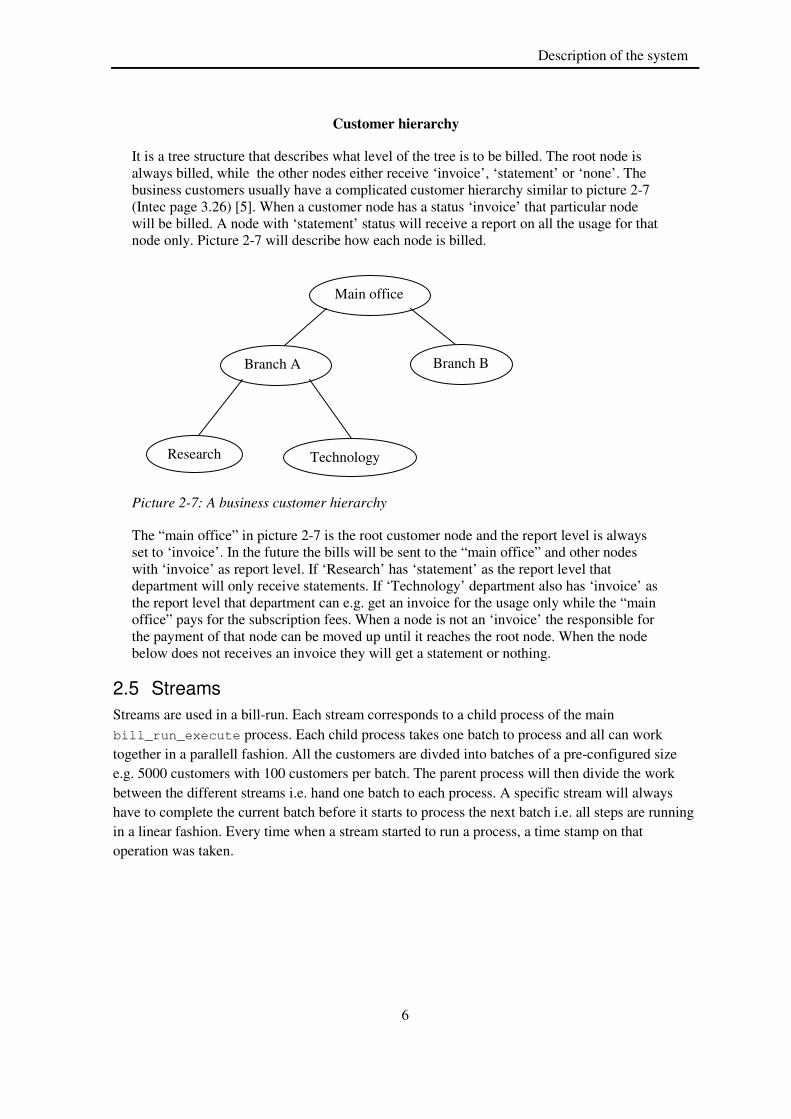
It is a tree structure that describes what level of the tree is to be billed. The root node is always billed, while the other nodes either receive ‘invoice’, ‘statement’ or ‘none’. The business customers usually have a complicated customer hierarchy similar to picture 2-7 (Intec page 3.26) [5]. When a customer node has a status ‘invoice’ that particular node will be billed. A node with ‘statement’ status will receive a report on all the usage for that node only. Picture 2-7 will describe how each node is billed.
Picture 2-7: A business customer hierarchy
The “main office” in picture 2-7 is the root customer node and the report level is always set to ‘invoice’. In the future the bills will be sent to the “main office” and other nodes with ‘invoice’ as report level. If ‘Research’ has ‘statement’ as the report level that department will only receive statements. If ‘Technology’ department also has ‘invoice’ as the report level that department can e.g. get an invoice for the usage only while the “main office” pays for the subscription fees. When a node is not an ‘invoice’ the responsible for the payment of that node can be moved up until it reaches the root node. When the node below does not receives an invoice they will get a statement or nothing.
2.5 Streams
Streams are used in a bill-run. Each stream corresponds to a child process of the main bill_run_execute process. Each child process takes one batch to process and all can work together in a parallell fashion. All the customers are divded into batches of a pre-configured size e.g. 5000 customers with 100 customers per batch. The parent process will then divide the work between the different streams i.e. hand one batch to each process. A specific stream will always have to complete the current batch before it starts to process the next batch i.e. all steps are running in a linear fashion. Every time when a stream started to run a process, a time stamp on that operation was taken.
Main office
Branch A Branch B
Research Technology

7
Theoretical background
Streams
S1
RGP BGP IGP Unit(time)
Picture 2-8: Single stream job
Picture 2-8 shows a simplified bill-run where each box symbolizes one unit of time and operation. With one stream, the RGP phase took two units, BGP took five units and the last IGP step took seven units of time. S1 is the stream that was used for running the whole bill-run operation and is the total number of all boxes. Total time is now 14 units.
Streams
S3
S2
S1
RGP BGP IGP Unit(time)
Picture 2-9: Bill-run with multiple streams
The multiple streaming option is used in a normal bill-run when running with multiple streams to increase the performance. Same jobs can be divided to run in a parallell fashion. When a bill-run has finished statistics about the bill-run can be obtained from the database or the Singl.eView client.
3 Theoretical background
Queueing theory can calculate the theoretical values for ideal utilization in a computer system. This helps the analyst to identify any future gains by using queueing theory formulas before investing funds in new equipment or performing new performance tests.
Spelling issues
“Queueing” or “Queuing” is the question? Both are right answers. The word “queueing” is more frequently used by queueing mathematicians and related people working in this field. While “queuing” is the preferred word for spell checkers and dictionaries according to Carry Millsap (2003) [1]. For further information check this webpage [8].
R B B I I I I R B B B I I I
R B I
R B I
R R
R R
R R
B B
B B
B B
B B
B
I I
I I I I R B B I I
R
B B B B I I
B B B B B B I I
I
I
R R I I

8
Theoretical background
For example if a company has plans for a system upgrade, the best way is not to buy the necessary equipment and run a test on it. If the tests for the new system proved that the performance has been decreased, it would have been cheaper to calculate the performance with some queueing formulas.
Understanding queueing theory would help the analyst to have a better understanding about response time. It shows clearly if the system is spending the time to process a job or is wasting the time in the queue. The formulas in this section are using the same notation as Millsap [1]. Response time can be illustrated with the formula below.
WSR += (3-1)
where R is response time, S is service time and W is the wait time. This equation was first introduced by Kolk, Yamaguchi and Viscusi (1999) [9]. The service time S is the time a job is in the system with the available resources working with a given task. The wait time W for a job is the waiting time for a resource to be accessible.
In queueing theory, λ is used to denote the mean arrival rate of jobs into the system divided by a time period. The notation A is the number of arriving jobs e.g. if a SQL statement executes four times in the system and the time T is per second, then the mean arrival time λ equals four statements per second coming to the system.
T
A=λ (3-2)
The test machine has eight processors and can be described as one system with eight parallel service units. The number of service units is denoted m in this project. In the test machine m for example is eight and the utilization for each CPU is denoted ρ also called traffic intensity. This value must be between 0 ≤ ρ < 1 for the queueing system to be stable. If ρ is larger than 1, the system will have more jobs than it can handle.
1<=µ
λρ
m (3-3)
The equation above is used to calculate ρ. The service rate is denoted by µ as:
µ = 1/S (3-4)
Where S is the average service time, µ is calculated from the jobs being processed as busy in the service unit, divided by the time when they are completed. This equation calculates e.g. the number of jobs a CPU can process (during) a given time. The probability for the number of jobs in the system Pn is calculated with the following formula (3-5) where n denotes the number of jobs.

9
Theoretical background
( ) ( )( )
( )
≥⋅
≤⋅
=
−+
=
−
−−
=
∑
mnp
mnn
mp
nm
m
i
m
p
mn
m
n
m
i
mi
n
ρ
ρ
ρ
ρρ
!
01!!
0
11
0
(3-5)
This assume that ρ < 1 equation (3-3).
The average number of jobs waiting in the queue is defined as ql . Where Cm is the Erlangs C
formula see equation (3-8).
( ) ρ
ρ
ρ
ρ
ρ
ρ
−=
−=
−=
+
11)1(! 22
)1(
0m
m
mm
q
Cp
m
mpl (3-6)
The number of jobs in the system is defined as l.
µ
λ
µ
λ
ρ
ρ+=+
−= q
m lC
l1
(3-7)
The time a job spends waiting in the queue is calculated from Erlangs C formula below.
−+−
=−
=
∑−
=
1
0 )1(!
)(
!
)()1(
!
)(
1 m
i
mi
m
mm
m
m
i
m
m
m
pC
ρ
ρρρ
ρ
ρ (3-8)
The expected time a job spends in the queue is denoted as wq.
λq
q
lw = (3-9)
The average time a job spends in the system w is calculated by the formula below.
( ) λµρλ
ρ
µ
qmlC
w +=−
+=1
1
1 (3-10)
Multiplying with λ on both side of the equation (3-10) and substituting with equation (3-7) gives equation (3-11).
λλ
λ
λ
µ
λλ
lwlw
lw
q=⇒=⇒+= (3-11)

10
Theoretical background
A computer can process a certain number of jobs in a given time. A job’s performance can be estimated with the Cumulative Distribution Function (CDF). The result from CDF will show the probability that the system can complete most of the jobs with the maximum tolerance value r. This is the parameter that is most important to the user.
3.1 Parameter explanation for the Excel tool
The notation for the number of parallel service units is defined as “M/M/m” which is a notation for a Markovian queueing system with m units or queues. The following notations are used in the tool made in Excel, for an explanation of it [1], see picture 3-1 on the next page. A short description about the parameters will be explained below.
The parameter m denotes the number of available service units that can process the jobs in the system. For example a computer with a number of built in hard drives or CPUs which can process the incoming jobs in a parallel way.
µ measures the number of jobs the system can process. The parameter q > 1 see equation (3-12).
S
q=µ (3-12)
rmax is the maximum users “tolerant” response time for the CDF calculation. CDF will calculate a probability, if all the jobs in the system can be finished in the specified time measured by seconds. This parameter can be changed by the user.
CDF is calculated with the formula below (Millsap page 234-235) [1].
( )( )
( ) ( )( )
( )( )rmqrqe
m
We
m
WmrFrRP
λµµ
ρρ
ρ−−− −
−−
−−−
−−
−−==≤ 1
11
011
11
)0(1)()( (3-13)
( ) ( )( )ρ
ρ
−−=
1!10 0
m
pmW
m
q
(3-14)
P0 can be acquired from equation (3-5) where n = 0.
An example for the tool: if the queueing system can finish the jobs with the current input parameter range from cell B5-B10, see picture 3-1.

11
Theoretical background
Picture 3-1: Queueing theory calculation tool in excel
This tool shows that 660 functions executed within one minute in cell B7 and the average arrival rate 11 functions per second in cell B21. The average service rate is two functions per seconds in cell B22. The average CPU utilization was 69% see cell B23. Roughly 84% of all the jobs completed the task within the one second of response time limit see cell B28. To acquire a higher rate of satisfaction a useful function in Excel, “goal seek” can attempt to calculate what the input parameter should be if one tries a higher satisfaction rate. In MS excel 2007 goal seek can be found under the ‘data’ tab by clicking “what if analysis”. Click goal seek, to get a 99% satisfaction enter the value in the “To value:” box, goal seek has been used by (Millsap och Holt 2003).
Picture 3-2: Goal seek in Microsoft Excel
12
Methods
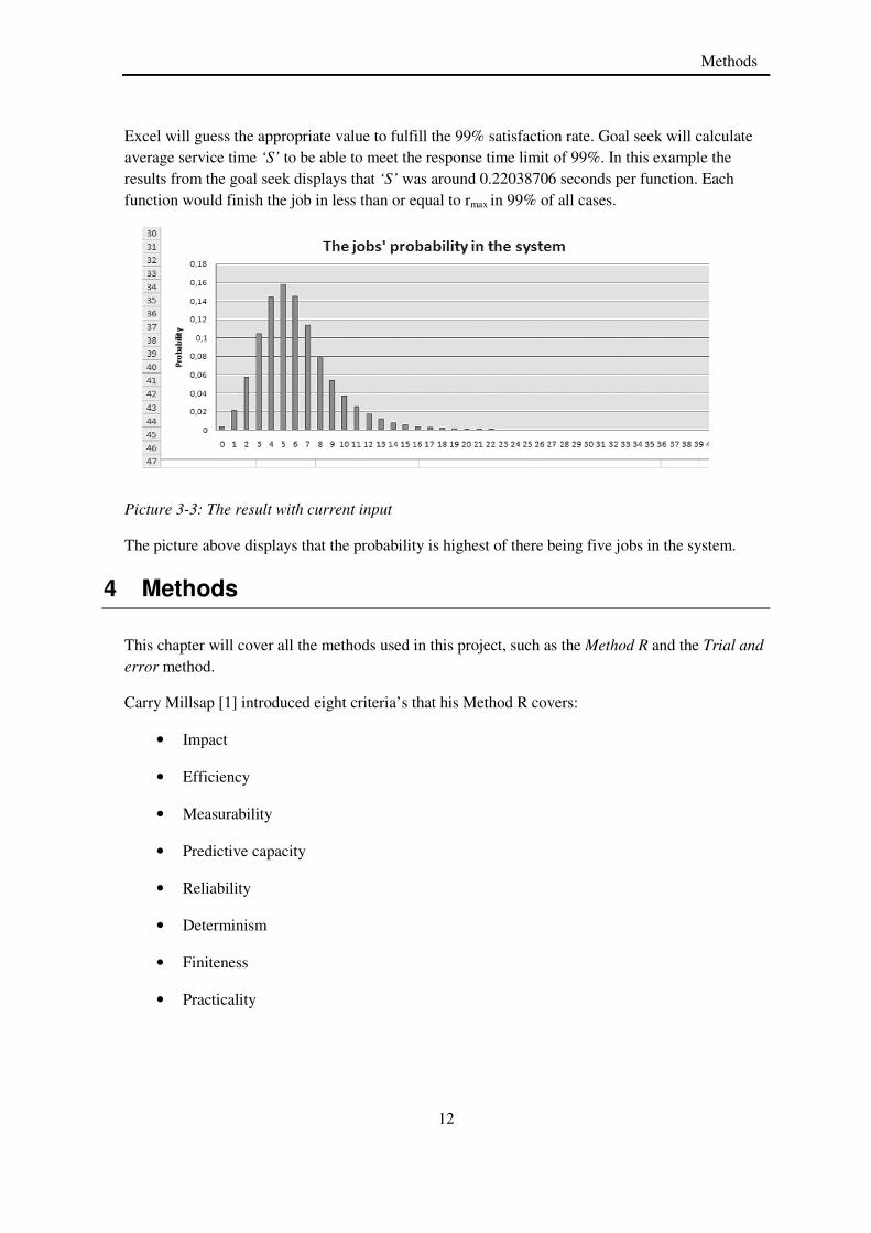
Excel will guess the appropriate value to fulfill the 99% satisfaction rate. Goal seek will calculate average service time ‘S’ to be able to meet the response time limit of 99%. In this example the results from the goal seek displays that ‘S’ was around 0.22038706 seconds per function. Each function would finish the job in less than or equal to rmax in 99% of all cases.
Picture 3-3: The result with current input
The picture above displays that the probability is highest of there being five jobs in the system.
4 Methods
This chapter will cover all the methods used in this project, such as the Method R and the Trial and
error method.
Carry Millsap [1] introduced eight criteria’s that his Method R covers:
• Impact
• Efficiency
• Measurability
• Predictive capacity
• Reliability
• Determinism
• Finiteness
• Practicality
13
Methods
4.1 Method R
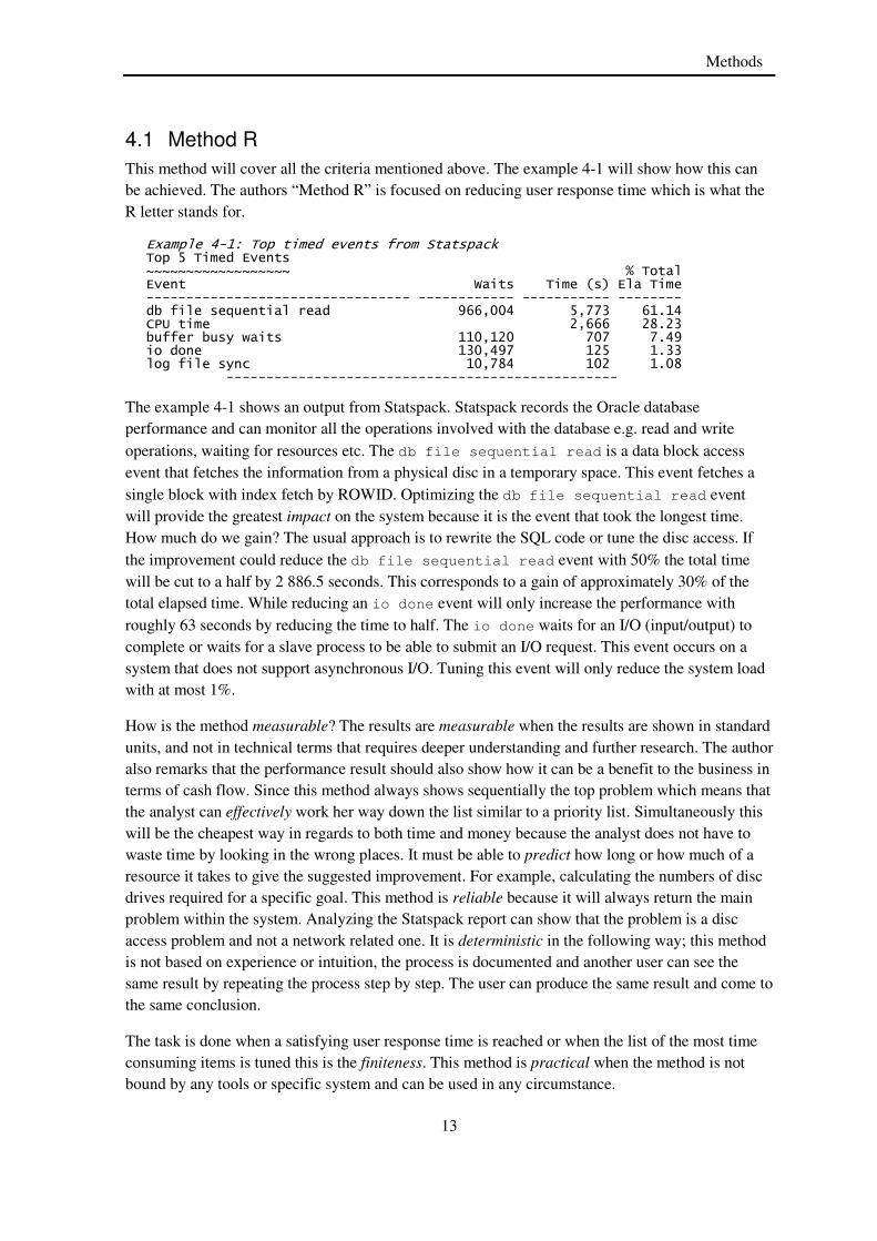
This method will cover all the criteria mentioned above. The example 4-1 will show how this can be achieved. The authors “Method R” is focused on reducing user response time which is what the R letter stands for.
Example 4-1: Top timed events from Statspack Top 5 Timed Events ~~~~~~~~~~~~~~~~~~ % Total Event Waits Time (s) Ela Time --------------------------------- ------------ ----------- -------- db file sequential read 966,004 5,773 61.14 CPU time 2,666 28.23 buffer busy waits 110,120 707 7.49 io done 130,497 125 1.33 log file sync 10,784 102 1.08 -------------------------------------------------
The example 4-1 shows an output from Statspack. Statspack records the Oracle database performance and can monitor all the operations involved with the database e.g. read and write operations, waiting for resources etc. The db file sequential read is a data block access event that fetches the information from a physical disc in a temporary space. This event fetches a single block with index fetch by ROWID. Optimizing the db file sequential read event will provide the greatest impact on the system because it is the event that took the longest time. How much do we gain? The usual approach is to rewrite the SQL code or tune the disc access. If the improvement could reduce the db file sequential read event with 50% the total time will be cut to a half by 2 886.5 seconds. This corresponds to a gain of approximately 30% of the total elapsed time. While reducing an io done event will only increase the performance with roughly 63 seconds by reducing the time to half. The io done waits for an I/O (input/output) to complete or waits for a slave process to be able to submit an I/O request. This event occurs on a system that does not support asynchronous I/O. Tuning this event will only reduce the system load with at most 1%.
How is the method measurable? The results are measurable when the results are shown in standard units, and not in technical terms that requires deeper understanding and further research. The author also remarks that the performance result should also show how it can be a benefit to the business in terms of cash flow. Since this method always shows sequentially the top problem which means that the analyst can effectively work her way down the list similar to a priority list. Simultaneously this will be the cheapest way in regards to both time and money because the analyst does not have to waste time by looking in the wrong places. It must be able to predict how long or how much of a resource it takes to give the suggested improvement. For example, calculating the numbers of disc drives required for a specific goal. This method is reliable because it will always return the main problem within the system. Analyzing the Statspack report can show that the problem is a disc access problem and not a network related one. It is deterministic in the following way; this method is not based on experience or intuition, the process is documented and another user can see the same result by repeating the process step by step. The user can produce the same result and come to the same conclusion.
The task is done when a satisfying user response time is reached or when the list of the most time consuming items is tuned this is the finiteness. This method is practical when the method is not bound by any tools or specific system and can be used in any circumstance.

14
The Project’s Work Process
4.2 Applying methods
The function analysis can be found in chapter five. The function optimization was chosen based on the elapsed time, core or internal functions and complexity. These parameters determined how the Method R was applied in the optimization work. Not all the points mentioned in Method R were covered but it was taken in consideration when the function optimization was performed. The impact point was the hardest point to cover because most of the changeable functions were internal ones. These functions usually were already fast enough and do not consume much in regards to response time. See the Top function section in chapter five for a comparison. The functions that were chosen for optimization purposes were recommended by the company’s supervisor and were chosen based on the function statistics that was gathered in this project.
The Method R was not the only method used in the project because in some cases it was harder to implement the Method R on some aspects of the project e.g. when running bill-runs. There is no good way to determine if the tests will turn out to be good or bad regarding results unless we are trying different configurations with a trial and error approach. All the bill-runs are tested in trial
and error fashion by running test after test with different settings. The Trial and error method was not the best method, in fact it was the worst method available, because there is no indication as to when these tests will end and it is hard to measure or predict the outcome of the results. To determine when the test will be finished the performance tests were divided into a smaller test scope e.g. running the machine on maximum settings and then reduce the settings until an acceptable result was reached. This method is the opposite of the Method R because all the criteria’s described for the Method R will probably fail in most points mentioned above with trial and error. The trial and error method cannot guarantee to identify the bottleneck and find the main problem directly which would provide with an unknown impact and reliability. It is very inefficient because usually all the test cases need to be examined, it is also very hard to determine when the work is done (finiteness). This method is also based on experience and assumptions which is not deterministic. This reason was also mentioned in Millsap’s book 2003 [1] when he compared these methods with each other. The Method R was applied in the function test only.
5 The Project’s Work Process
This chapter is divided into several parts and the major focus was on the project’s work process and gives an overview of the performance tests and its configurations. Further reading will introduce the reader to Statspack and how it works. Function optimization results can also be found in this chapter.
5.1 Preparations
A normal bill-run takes approximately twenty hours to finish in the production machine. The current setting for a bill-run today is using the default configuration. The test machine’s default setting today is using three of each RGP, BGP and IGP processes. The test environment was used in order to collect the statistics described in chapter two. There is a big difference in hardware between the two machines e.g. the production machine which have 40 CPUs installed compared to the test environment’s eight CPUs. A normal size for a bill cycle is around hundred thousand customers but this varies from cycle to cycle. Because of the hardware difference the bill cycles’ size had to be decreased compared to the production machine’s settings in order to be able to

15
The Project’s Work Process
complete a bill-run in reasonable time. In the first part’s tests, the bill cycles’ size was set to around 5 000 customers and this equals five percent of a normal bill cycle. Bill cycle statistics were collected in the first part of the performance tests. A total of three stages of performance tests were performed. A default setting for the RGP, BGP and IGP processes was set based on the Intec documentations [4] [5]. Ten streams with 100 customers as the batch size was used in the first part.
Table 5-1: Bill cycles names and sizes for the first part’s bill-run
Bill cycle Number of
customers
ID Total
Service
Avg service
/cust
Max
service
Min
service
Denmark Consumer 4 5001 DC4 7097 1.419116 6 0
Denmark Business 2 5001 DB2 15943 3.187962 205 0
Sweden Consumer 6 5001 SC6 6179 1.235553 5 0
Sweden Business 3 4058 SB3 11058 2.724988 177 0
Sweden Business 4 1 SB4 2569 2569 2569 0
Table 5-2: Second part’s bill cycles
Bill cycle Number of
customers
ID Total
Service
Avg service
/cust
Max
service
Min
service
Denmark Consumer 4 100 DC4 135 1.35 5 0
Denmark Business 2 100 DB2 290 2.9 21 0
Sweden Consumer 6 100 SC6 112 1.12 2 0
Sweden Business 3 100 SB3 230 2.3 20 0
Table 5-3: Third part’s bill cycles
Bill cycle Number of
customers
ID Total
Service
Avg service
/cust
Max
service
Min
service
Denmark Consumer 4 2000 DC4 2797 1.3985 6 0
Denmark Business 2 2000 DB2 7422 3.711 81 0
Sweden Consumer 6 2000 SC6 2450 1.225 6 0
Sweden Business 3 2000 SB3 3389 1.6945 78 0
*Sweden Business 4 1 SB4 3132 3132 3132 0

16
The Project’s Work Process
In table 5-1 to 5-3 is the bill cycles names that was used in the tests. Before a bill-run was started a script was used to reset and start the statistic collection with ‘getstats’ [10]. Another script was used to output the statistics to files. Part of the statistic results can be found in appendix B. In the second tests, 100 customers were used as the input size and batch size was ten. The number of streams varied between the executions. In the third part’s tests 2000 customers’ bill cycles were used and were running with three streams. The batch size was decreased because of the bill cycles size during that phase.
5.2 Server Configuration Overview
A standard bill-run has default configuration settings and uses a set of streams where the bill_run_execute process spawns a child for each stream. At the RGP step the number of streams should be equal to the number of CPUs. The number of streams has a suggested maximum limit of 1.5 times the number of installed CPUs at the BGP stage. In the IGP phase the number of streams should be around 1.1 to 1.2 times the number of CPUs and this could improve the performance according to Intec page 10.2-10.6 [4]. The test that was performed did not show any improved performance at the first part compared to the baseline tests, however in the second and third part, the performance tests showed very good results.
Today the company uses the default server configuration. Investigating if it was possible to measure any performance gain by changing the process setting was done. Each of the RGP, BGP, and IGP phases can have a unique setup. Cycles with many customer nodes, services or events can have their performance improved in the BGP step by configuring the BGP settings. Changing the parameter CUSTOMER_CHILD_PROCESSES (CCP), SERVICE_CHILD_PROCESSES (SCP), NODE_CHILD_PROCESSES (NCP) and EVENT_CHILD_PROCESSES (ECP) from the default value ’0’ will start additional processes. Each additional process that has been spawned may improve performance at the BGP step but this depends on the bill cycles structure and will consume more resources like memory. Changing the CUSTOMER_CHILD_PROCESSES will process more accounts or customers at the root level. This parameter will only spawn the amount of processes equal to the value of CUSTOMER_CHILD_PROCESSES. Editing the NODE_CHILD_PROCESSES will spawn more child processes.
Picture 5-1: The BGP process relations
BGP server
CCP
CCP
CCP
NCP
NCP
SCP
SCP
SCP
SCP
ECP
ECP
ECP
ECP
…
…
…
…

17
The Project’s Work Process
The number of spawned BGP processes is explained with help from picture 5-1 and example 5-1.
Example 5-1 Part of the BGP configuration file
1. [BGP.1] 2. Name=BGP1 3. Group=6 4. CUSTOMER_CHILD_PROCESSES=0 5. NODE_CHILD_PROCESSES=0 6. SERVICE_CHILD_PROCESSES=0 7. EVENT_CHILD_PROCESSES=0
Example 5-1 is accessed through Singl.eView’s configuration item or changed with the following UNIX command.
> cfg -f bgp.cfg
The –f flag specifies what configuration file to be used, in this example is the“bgp.cfg” file. In the experiments line five and six was changed frequently for the first part’s tests. Line four was used in some test during the third test phase. In consumer cycles the customer hierarchy is usually one customer with one service and in these cases using batch streaming is more effective than changing the BGP settings. Batch streaming is equal to using default setting with a set of streams and batch size in Singl.eView (Intec page 10-3) [4]. The default settings can be found at appendix C file C-1. To calculate the number of spawned BGP processes for the test machine, a stable amount of total active child processes were around 8-12 processes that includes the IGP child processes. When 12 or more processes are spawned some bill-runs can still manage to complete the task but a socket error was found for these bill-runs, see chapter 8.1 about the problem. The test machine has three BGP processes e.g. line six in example 5-1 is set to 2. Each BGP server would spawn three processes in total because the CCP and NCP are spawned as one BGP child process observed with the UNIX command ps. Picture 5-2 describes the total amount of spawned processes.
Picture 5-2: The total number of spawned processes with SCP set to 2
The number of total child processes is 9 processes in total, because the CCP and the NCP processes count as one child process. When 0 or 1 is set in the BGP configuration file, the system spawns
BGP server CCP NCP
SCP
SCP
BGP server
CCP NCP
SCP
SCP
BGP server CCP NCP
SCP
SCP

18
The Project’s Work Process
them together as one process except for the process with a value larger than 1. The ECP process that is furthest away from the BGP server would not be spawned because the value is less than 2. Same situation occurs when the NCP parameter is set the SCP and the ECP processes would not be spawned.
Table 5-4: List of abbreviations of the BGP configuration items
BGP item Abbreviation Default value Customer Child Processes CCP 0 Node Child Processes NCP 0 Service Child Processes SCP 0 Event Child Processes ECP 0
The IGP configuration file has a parameter called MAX_CHILD_PROCESSES, changing this will generate more child processes for IGP. The number of total child processes is the number of IGP servers multiplied with the value from MAX_CHILD_PROCESSES.
Multiprocessing with different BGP configurations can be used when dividing the cycle into different sets. The criteria could be grouped by active services or events that a customer has. These steps are necessary to configure a multiprocessing configuration.
• Create profile tables
• Use at least two instances of BGP configurations
• Change the Tuxedo server configuration
• Update the bill cycle
Creating a profile for the bill cycles identifies the characteristic of the cycle. The profile will summarize the number of customers, customer nodes, charges, services and active services in a specified period. The code for creating the profiling table is shown in appendix C. The first two lines at code 13-1 need to be changed. At BGP configuration level create another BGP configuration file similar to example 5-1. The second file was changed mainly at the node child processes (NCP) and service child processes (SCP) parameters. The file created was used to update the configuration item in Singl.eView that is used by the trebgp process as specified in the ubbconfig file. The example in appendix C file C-2 shows how a second configuration file can be written. To generate more trebgp servers (BGP processes) the file named “ubbconfig.tpl” need to be changed and can be accessed from the “config” directory on the UNIX server. This is the path for the test environment.
/sv/sv_pro2/data/server/config
Inside the file there is a section marked with BILLING used for all the RGP, BGP and IGP setup. Adding example 5-1 in the file will start three extra trebgp tuxedo servers advertising the service biBGPHighVol:biFnEvaluate using the configuration as specified by BGP2 configuration item. The original settings can be found in appendix C under Files. The below setting will start three additional trebgp processes, which uses the configuration as determined by the BGP2 configuration item. In addition the three normal trebgp processes are still there, which will use the

19
The Project’s Work Process
setting of the BGP1 configuration. This will enable the possibility to have different customers to be processed by different BGP settings based on their profile.
Example 5-2: This is a piece of configuration code from ubbconfig.tpl file. Additional trebgp for enable billing configuration for high volume trebgp SRVGRP=BILLING SRVID=230 RESTART=Y MAXGEN=5 CLOPT="-s biBGPHighVol:biFnEvaluate -- BGP2" MIN=3 MAX=6 SEQUENCE=6
The max value is only a threshold to prevent the system from spawning any more processes than the system has resources for. Setting the MAX parameter will not spawn any BGP2 processes automatically, to utilize the desired number of processes it requires that the MIN parameter be changed manually in the file i.e. any additional servers above the MIN level needs to be started manually and are not started dynamically by the system. When the server setting has been set, the next step is to configure the bill cycle. The SQL code in example 5-3 is used for fetching the number of active services for every customer in the test table hmw_testsc6 (SC6) with more or equal to four services. The table hmw_testsc6 was a temporary table which contained the 5000 customers i.e. the sample customers used for performance testing of the bill cycle in question. All the test tables were destroyed when a new production clone was taken at the end of the month. A production clone is the backup data that was transferred from the production machine to the test machine.
Example 5-3: Selecting the number of active service select tcp.* from testuser.customer_profile tcp, testuser.hmw_testsc6 tdata where tcp.customer_node_id = tdata.customer_node_id
and active_service_count >= 4 order by nvl(charge_count, 0) desc;
This SQL code was an easy way to determine how many of the total active services to be divided between the trebgp processes using BGP1 or BPG2 configuration. The number of services should be changed to an appropriate value depending on what proportion to be divided into. The testuser table space needs to be changed to fetch the relevant data.
The last step was to save the updated customers by executing the update SQL code in example 5-4.
Example 5-4: A SQL update code to get the costumer with more or equal to four services.
1. update customer_node_history cnh 2. set billing_configuration_code = 2 3. where customer_node_id in ( 4. select tdata.customer_node_id 5. from testuser.hmw_testsb3 tdata, testuser.customer_profile tcp 6. where tcp.customer_node_id = tdata.customer_node_id 7. and tcp.active_service_count >=4 );
This code piece set the billing_configuration_code value to two because the biBGPHighVol:biFnEvaluate has identification code two i.e. the code determines which BGP configuration that should be used during the BGP phase. All the customers with four or more active services will be affected. Line five with testuser schema also needs to be changed like example 5-3. The billing_configuration_code is used to identify which setting of the BGP that
20
The Project’s Work Process
should be used for a specific customer in this case BGP2 settings will be applied to the customers with four or more services.
5.3 Performed Configuration Tests
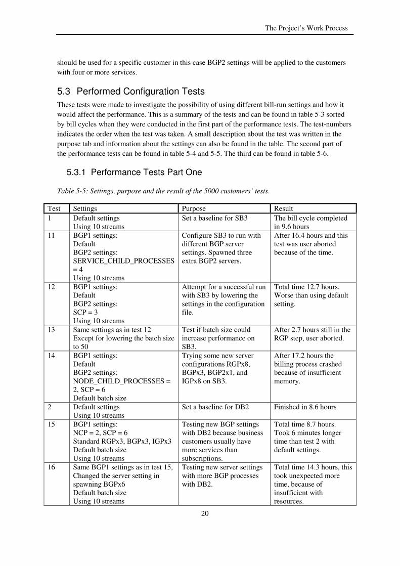
These tests were made to investigate the possibility of using different bill-run settings and how it would affect the performance. This is a summary of the tests and can be found in table 5-3 sorted by bill cycles when they were conducted in the first part of the performance tests. The test-numbers indicates the order when the test was taken. A small description about the test was written in the purpose tab and information about the settings can also be found in the table. The second part of the performance tests can be found in table 5-4 and 5-5. The third can be found in table 5-6.
5.3.1 Performance Tests Part One
Table 5-5: Settings, purpose and the result of the 5000 customers’ tests.
Test Settings Purpose Result 1 Default settings
Using 10 streams Set a baseline for SB3 The bill cycle completed
in 9.6 hours 11 BGP1 settings:
Default BGP2 settings: SERVICE_CHILD_PROCESSES = 4 Using 10 streams
Configure SB3 to run with different BGP server settings. Spawned three extra BGP2 servers.
After 16.4 hours and this test was user aborted because of the time.
12 BGP1 settings: Default BGP2 settings: SCP = 3 Using 10 streams
Attempt for a successful run with SB3 by lowering the settings in the configuration file.
Total time 12.7 hours. Worse than using default setting.
13 Same settings as in test 12 Except for lowering the batch size to 50
Test if batch size could increase performance on SB3.
After 2.7 hours still in the RGP step, user aborted.
14 BGP1 settings: Default BGP2 settings: NODE_CHILD_PROCESSES = 2, SCP = 6 Default batch size
Trying some new server configurations RGPx8, BGPx3, BGP2x1, and IGPx8 on SB3.
After 17.2 hours the billing process crashed because of insufficient memory.
2 Default settings Using 10 streams
Set a baseline for DB2 Finished in 8.6 hours
15 BGP1 settings: NCP = 2, SCP = 6 Standard RGPx3, BGPx3, IGPx3 Default batch size Using 10 streams
Testing new BGP settings with DB2 because business customers usually have more services than subscriptions.
Total time 8.7 hours. Took 6 minutes longer time than test 2 with default settings.
16 Same BGP1 settings as in test 15, Changed the server setting in spawning BGPx6 Default batch size Using 10 streams
Testing new server settings with more BGP processes with DB2.
Total time 14.3 hours, this took unexpected more time, because of insufficient with resources.

21
The Project’s Work Process
17 BGP1 settings: NCP = 3, SCP = 4 Default server setting Batch size 70 Using 10 streams
Testing with new BGP settings on DB2.
No improvement found the test was user aborted after 16.9 hours. Insufficient with memory.
3 Default settings Using 10 streams
Set a baseline for DC4 Finished in 7.7 hours
4 Default settings Using 10 streams
Set a baseline for SC6 Finished in 6.3 hours
5 Default settings Using 10 streams
Set a baseline for SB4 Finished in 10.1 hours BGP step took 2.1 hours IGP step took 8.8 hours
6 BGP1 settings: NCP = 2 and SCP = 6 Using 10 streams
Change the BGP settings for SB4. This bill cycle is special because there is only one customer node with many services by creating more service child processes might increase performance
9.6 hours and this gave increasing performance with 30 minutes. BGP step took 1.4 hours, gained 42 minutes compared to test 5.
7 BGP1 settings: NCP = 2, SCP = 4, EVENT_CHILD_PROCESSES = 2 Using 10 streams
Test SB4 to see if setting the ECP will increase performance because the cycle has many events. Running from the beginning to the BGP step as finish line.
This step was user aborted because total time was 4.7 hours and it was still running. No performance gained compared to test 6.
8 BGP1 settings: NCP = 1 and SCP = 8 Using 10 streams
Changed the setting in SB4, run from the beginning to the BGP step same as in test 7.
Total time 1.4 hours. The BGP step took 1.3 hours to complete. Four minutes gained compared to test 6.
9 BGP1 settings: NCP = 1 and SCP = 12 Using one stream
Tested with 12 SCP because the BGP step can be 1.5 times the number of CPUs on SB4
Test failed after 9.2 hours and the process crashed because of insufficient memory.
10 BGP1 settings: NCP = 2, SCP = 2 IGP settings: MAX_CHILD_PROCESSES = 3 Using 10 streams
Trying with new settings by using BGP and IGP configuration simultaneously on SB4
Total time 10.3 hours BGP step took 2.1 hours IGP step took 8.0 hours Gained 48 minutes compared to test 5’s IGP step. But overall time took longer than test 5 and 6.
5.3.2 Performance Test Part Two
Running the 5000 customers’ bill-run involved some crashes and memory issues. A new test with smaller size of 100 customers’ was performed and the default settings are same as before on the server configuration settings. Batch size has been lowered to ten. SB4 cycle was not tested due to the number of customers.

22
The Project’s Work Process
Table 5-6: Settings, purpose and the result of a smaller (100) bill cycles
Test Settings Purpose Result 1 Default settings:
Batch size 10 Using 8 streams
Set a baseline time for maximizing the CPU usage on SB3
Bill-run completed in 26.8 minutes
6 Default settings Using 8 streams
Changed a function fH3G_GetGLCodeName& running on SB3
Finished at 25.6 minutes, gained 1.2 minutes compared to test 1, gained 4%
9 Default settings Using 8 streams
Changed a new function fH3G_Bil_VolumeCharge# running on SB3 all previous function changes are still active
Finished at 22.1 minutes, gained 3.5 minutes compared to test 6, gained 13.7%
13 IGP MAX_CHILD_PROCESSES = 8 Using 8 streams
Testing on SB3 with same setting as test 12 all previous function changes are still active
Finished at 15 minutes, gained 7.1 minutes compared to test 9 a better result with approximately 32%
2 Default settings Using 8 streams
Set a baseline time for maximizing the CPU usage on SC6
Bill-run completed in 13.4 minutes
7 Default settings Using 8 streams
Changed a function fH3G_GetGLCodeName& running on SC6
Finished at 13.2 minutes, gained 0.2 minutes compared to test 2, 1.5% gained
11 Default settings Using 8 streams
The functions from test 10 are restored back and another change with a new function fHi3G_Inv_GetPackageCount& was tested on SC6 all previous function changes are still active
Finished at 10.3 minutes, gained 2.9 minutes compared to test 7, gained 22%
15 IGP MCP = 8 Using 8 streams
Testing on SC6 with same setting as test 12 all previous function changes are still active
Completed in 9 minutes, gained 1.3 minutes compared to test 11,

23
The Project’s Work Process
gained 12.6% 3 Default settings
Using 8 streams Set a baseline time for maximizing the CPU usage on DC4
Bill-run completed in 13.1 minutes
5 Default settings Using 8 streams
Changed a function fH3G_GetGLCodeName& running on DC4
Finished at 9.3 minutes, gained 3.8 minutes compared to test 3, gained 29%
10 Default settings Using 8 streams
Changed two new functions fH3G_NUC_RecurringChgElig& and fHi3G_NUC_CampaignRecurringChgElig& tested with DC4 all previous function changes are still active
Finished at 16.3 minutes and this test took 7 minutes longer than test 5
14 IGP MCP = 8 Using 8 streams
Testing on DC4 with same setting as test 12 all previous function changes are still active
Completed in 9.4 minutes not better result than test 5 but a performance gain compared to test 3 with 28%
4 Default settings Using 8 streams
Set a baseline time for maximizing the CPU usage on DB2
Bill-run completed in 12 minutes
8 Default settings Using 8 streams
Changed a new function fH3G_Bil_VolumeCharge# running on DB2 all previous function changes are still active
Finished at 10.7 minutes, gained 1.3 minutes compared to test 4, gained almost 11%
12 IGP MCP = 8 Using 8 streams
Testing new server configuration settings on DB2 and set the limit of MCP equal of the number of CPUs’ all previous function changes are still active
Finished at 10.1 minutes, gained 0.6 minutes compared to test 8 almost gained 6%
The last test with a small input size showed promising performance gain and a new analysis was performed that resembles the production machine. The production machine is running with a predefined setting of 32 instances of the following processes: RGP, BGP and IGP. The production machine has 40 build in CPUs as mentioned before. The server configuration setting has been set to

24
The Project’s Work Process
the default values. In the next table the tests are performed with the test machines default values i.e. three instances of each processes of: RGP, BGP and IGP. The batch size was same as the previous test which was number ten. Three streams will be used because the production machine uses 32 streams in a bill-run operation. All the function improvements before were still active for the upcoming test. There were a few unnecessary tariffs concerning the discounts that were triggered for all the customers. The discounts are not applicable for all the customers and therefore some of them were removed. But the function and tariff improvements were removed when the next clone was taken i.e. in part three’s performance test.
Table 5-7: A further analysis on the server configuration settings
Test Settings Purpose Result 1 Default settings:
with 3 RGP, 3 BGP, 3 IGP, batch size 10, 3 streams
Removed the following unnecessary tariffs: tH3G_NUC_1A_Musik_MRC# tH3G_NUC_1A_ProductMRC# tHi3G_NUC_1B_DeviceProductMRC# tHi3G_NUC_1B_PackageCampaignMRC# tHi3G_NUC_1B_PackageCampaignMRCThreshold# tHi3G_NUC_1B_PackageCampaignMRC_Arrears# set a baseline for SB3
Finished at 25.7 minutes
5 IGP MCP = 3 Batch size 10 Using 3 streams
The IGP Max Child Processes settings that resembles the production machine tested with SB3
Finished in 9.7 minutes and gained 16 minutes compared to test 1 over a 62% of improvement
11 BGP SCP = 3 IGP MCP = 3 Batch size 10 Using 3 streams
Testing the same settings on the SB3 cycle Took 21.2 minutes which was better than the default run but the only using the IGP settings alone gave much better performance, 18% gain compared to test 1
13 BGP SCP = 3 Batch size 10 Using 3 streams
Testing with same setting as in test 9 for SB3 Completed in 24 minutes, small performance gain when comparing with default setting, 7% gain compared to test 1
2 Default settings Set a baseline for DC4 Finished at 19.7 minutes
8 IGP MCP = 3 Batch size 10 Using 3 streams
Using the same settings for DC4 Completed in 11.5 minutes, gained 8.2 minutes almost 42% of improvement

25
The Project’s Work Process
compared to test 2 10 BGP SCP = 3
IGP MCP = 3 Batch size 10 Using 3 streams
Testing both the BGP and IGP settings simultaneously for DC4
Finished at 11 minutes slightly better than test 8, total gain 56% compared to test 2
14 BGP SCP = 3 Batch size 10 Using 3 streams
Testing with same setting as above with DC4 Completed in 19.2 minutes, small performance gain when comparing with default setting
3 Default settings Set a baseline for SC6 Completed in 16.1 minutes
6 IGP MCP = 3 Batch size 10 Using 3 streams
Using the same settings for SC6 Finished in 7.4 minutes, gained 8.7 minutes compared to test 2 improved with 54%
12 BGP NCP = 3 Batch size 10 Using 3 streams
Testing the node child process to see if there is anything to gain by changing this parameter for SC6
Failed after 21.5 minutes found a core dump file one process hang the entire bill-run process
4 Default settings Set a baseline for DB2 Completed in 18.2 minutes
7 IGP MCP = 3 Batch size 10 Using 3 streams
Using the same settings for DB2 Finished at 12.6 minutes, gained 5.6 minutes improved the result with around 30% compared to test 4
9 BGP SCP = 3 Batch size 10 Using 3 streams
Testing with the BGP Service Child Process server settings to see if the business customers can profit from this change for DB2
Completed in 6 minutes, gained 12.2 minutes improved with 67% compared to test 4
5.3.3 Performance Test Part Three
The purpose of part three’s performance tests was to confirm the results from part two. This will ensure that the result from part two’s test is more reliable when testing with more customers. In this session all the tests were performed with the same default setting as from part two i.e. three streams with three processes of each respective type RGP, BGP and IGP. Batch size was 50 customers per batch and the tests were analyzed with the bill cycles in table 5-5. Each month a copy of the data

26
The Project’s Work Process
from the production machine has been copied to the test environment. Before part three’s tests an update on the test environment was made from the production machine. All the functions that have been previously changed were lost, but backup of the changes was stored as files and in the development machine UAT2 as well.
Table 5-8: Performance test with 2000 customers
Test Settings Purpose Result 1 Default settings
Using 3 streams 50 batch size
Set a baseline for SB3 The bill cycle completed in 4.4 hours
2 IGP 3xMAX_CHILD_PROCESSES Using 3 streams
See if the MCP parameter can improve the performance for SB3
Finished in 2.9 hours, gained 1.5 hours, 34% of improvement compared to test 1.
9 IGP 3xMCP BGP 3xSERVICE_CHILD_PROCESSES
Testing how BGP and IGP would affect a business cycle (SB3).
Finished in 3.5 hours, gained 53min compared to test 1, 20% improvement.
10 BGP 3xSCP Using 3 streams 50 batch size
Trying with SCP parameter alone on SB3
Aborted after 16.5 hours, no performance gain, -275% compared to test 1. One of the BGP process died stalled the system
11 BGP 3xSCP Using 3 streams 200 batch size
Trying with a bigger batch with same settings as test 10 on SB3
Bill-run finished 11.8 hours, no performance gain, -168% compared to test 1. All the processes survived but due to too many spawned processes the bill-run took longer time to finish. Increasing the batch size lowered the chance to process crash.
12 BGP 2xSCP Using 3 streams 50 batch size
Lowering the SCP parameter and conduct another performance test for SB3
Finished in 3.6 hours gained 47.6 minutes, 18% performance gain compared to test 1.
13 BGP 2xCCP Using 3 streams 50 batch size
Trying another BGP parameter the Customer Child Process for SB3 cycle
Finished in 2.6 hours gained 1.7 hours and 41% in performance boost compared to test 1.
14 BGP 2xCCP IGP 2xMCP Using 3 streams 50 batch size
Since test 13 finished with great result trying to combine a BGP and IGP setting for SB3 cycle
Finished in 2.2 hours gained 2.2 hours, 50% of performance boost comparing with test 1

27
The Project’s Work Process
3 Default settings Using 3 streams 50 batch size
Set a baseline for DC4 Finished in 3.8 hours.
4 IGP 3xMCP Using 3 streams 50 batch size
Same purpose as test 2 but testing with DC4 cycle
Finished in 2.3 hours, gained 1.4 hours, 39% of improvement compared to test 3.
15 BGP 2xCCP Using 3 streams 50 batch size
Since test 13 gave good result on SB3 a test for DC4 was also conducted
Finished in 2.4 hours, gained 1.5 hours, 37% of performance lift compared to test 3.
16 BGP 2xCCP IGP 2xMCP Using 3 streams 50 batch size
Combining the IGP and BGP setting for DC4
Finished in 1.8 hours, gained 2 hours, 53% of performance gain compared to test 3.
5 Default settings Using 3 streams 50 batch size
Set a baseline for SC6 Finished in 2.7 hours.
6 IGP 3xMCP Using 3 streams 50 batch size
Testing MCP parameter for SC6
Finished in 2.0 hours, gained 40 min, 26% of improvement compared to test 5.
17 BGP 2xCCP Using 3 streams 50 batch size
Testing CCP parameter for SC6
Finished in 1.9 hours, gained 46 minutes, 30% of performance gain compared to 5.
18 BGP 2xCCP IGP 2xMCP Using 3 streams 50 batch size
Testing the BGP and IGP combination for SC6
Finished in 1.6 hours, gained 1.1 hours, 41% gain compared to test 5.
7 Default setting Using 3 streams 50 batch size
Set a baseline for DB2 Finished in 5.4 hours
8 IGP 3xMCP Using 3 streams 50 batch size
Testing MCP for DB2 Finished in 4.2 hours, gained 1.2 hours, 22% of improvement compared to test 7.
19 BGP 3xSCP Using 3 streams 200 batch size
Trying this setting with a larger batch for DB2
Completed in 6.2 hours, took more than 48 minutes compared to test 7, degraded the performance with -15%.
20 BGP 2xCCP Using 3 streams 50 batch size
Analyzing if the CCP parameter can have positive effect on the DB2 cycle
Finished in 4.9 hours, gained 26 minutes, 9% of performance boost compared to test 7.
21 BGP 2xCCP IGP 2xMCP Using 3 streams 50 batch size
Combining the BGP and IGP settings for DB2
Finished in 3.2 hours, gained 2.1 hours with 41% boost compared to test 7.

28
The Project’s Work Process
During the third performance test the Sweden Business 4 (SB4) cycle was analyzed and tested with different parameters during the first test phase. The number of tested customers in the other cycles was not enough to conclude that the setting would work for the whole bill cycle. That flaw was not possible to find in this cycle, because it was tested with the same setting and with the same amount of customers as the production machine. If a performance boost was discovered with the test machine, it is a very likely that same settings can be useful in another environment as well. In the third performance phase the cycle’s total services have been changed during these passed months and have been increased from 2569 services to 3132 services. The SB4 cycle has only one customer but has a large customer hierarchy with many customer nodes and could not be run with more than one stream and the batch size was irrelevant as well. This cycle spent approximately 70% of the time in the IGP phase.
Table 5-9: Test results for SB4
Test Settings Purpose Result 1 Default setting
Using 1 stream 50 batch size
Set a baseline for SB4 Finished in 12.0 hours
2 BGP 3xSCP IGP 3xMCP Using 1 stream 50 batch size
Using one stream bill-run also means that more child processes could be spawned for SB4
Finished in 11.5 hours and gained 30 minutes a performance boost of 4%. During the test only one MCP child was utilized which was strange.
3 BGP 4xNCP IGP 6xMCP Using 1 stream 50 batch size
Spawn more child processes to see if it will boost performance for SB4
Finished in 11.9 hours a very minor performance boost of 4.5minutes with 0.6% gain compared to test 1.
5.4 Function analysis
In each bill-run a getstats command was used to gather statistics on the following Tuxedo servers’: trergp, trebgp, treigp, trenodb, trerwdb and trerodb. All the services that require no database operations are done with trenodb which stands for non database server. The trerodb handles all the read only operations from the database and the trerwdb handles the read and write operations from the database. Every function that has been used has been picked up by getstats [10].
5.5 Top functions
The functions are measured in seconds (s) or in milliseconds (ms). The top functions for a specific phase can be found in appendix B and it is measured with default configuration settings. A summary of all the top functions can be divided into two groups. Group one is the core functions that where delivered with Singl.eView and internal functions that the company developed itself.

29
The Project’s Work Process
Table 5-10: Top core functions
Function name Max elapsed
time (s)
Phase Bill
cycle
biInvoiceImageGenerate& 85545.45 RODB SB3
biInvoiceGenerate& 73034.22 RODB DB2
InvoiceGenerate& 61738.78 BGP DB2
biRentalGenerate& 19461.08 RODB DB2
RentalGenerate& 11784.71 RGP DB2
biServiceFetchByName?[] 3084.68 RGP DB2
SQLQuery& 2816.60 IGP SB3
Table 5-10 shows the most time consuming functions taken from appendix B i.e. from the first part of the performance tests. The functions biInvoiceImageGenerate& are used for making invoice images (Intec page O-416) [11]. The second function in the list is biInvoiceGenerate& used for error handling and generates invoices, when used in the BGP step it limits the access to a certain customer during the billing process (Intec page O-410) [11]. This function is a wrapper function for the InvoiceGenerate& function (Intec page N-390) [12]. InvoiceGenerate& has the same functionality as the biInvoiceGenerate& but returns a different value. The biRentalGenerate& is also a wrapper function to RentalGenerate& and is similar to biInvoiceGenerate& (Intec page N-559) [11]. This function calculates the subscription fees or checks for any changes in the root customer node list. The next function biServiceFetchByName?[] gets the information about the service from a cache stored in the system (Intec page O-591) [11]. This function SQLQuery& runs and fetches the SQL statements (Intec page N-615) [12]. The core functions are the most consuming group of functions and it is not recommended to change these code pieces because it can easily affect the other parts of the billing system. But changing the internal functions will also affect the core functions in both positive and negative ways e.g. the SQLQuery is frequently called from functions developed locally to execute SQL statements thus a change to the SQL statement in a locally developed function may improve the performance significantly and thus also improve the performance displayed for the core functions.
Table 5-11: Top internal functions
Function name Max elapsed
time (s)
Phase Bill
cycle
fHi3G_Inv_GetSubString$ 1602.50 BGP SB3
fH3G_SplitString$[] 1244.01 BGP SB3

30
The Project’s Work Process
fH3G_ProductNames2Ids$[] 659.40 BGP DB2
fHi3G_InvoicePrint& 639.74 RODB DB2
fHi3G_Inv_GetSubStr$ 596.87 BGP DB2
fH3G_SearchMethod& 530.11 IGP SB3
fHi3G_Inv_AggregateUsageDet
ails&
498.76 IGP DB2
Table 5-11 shows the internal functions that the company has written, therefore can change, statistics taken from the first part’s performance tests. The slowest function fHi3G_Inv_GetSubString$ took 26.71 minutes (1602.50s). To improve the performance of this function is not easy since each execution is very quick but is called many times. To improve the performance the algorithm needs to be changed to actually reduce the numbers of function calls to this function i.e. also edit every function that called this function. Changing the storage type to reduce string comparisons will also provide with a performance boost, but extensive work is required to change everything involved in this function. No improvement to this function has been found so far.
The fH3G_GetGLCodeName& code has been optimized in the BGP phase. This function gets a string value and stores the result in a cache. Before the optimization, this function fetched the information (GLCode) from the database by calling the SQLQuery& function repeated times. The value that was fetched was stored in a cache in the trebgp process that was cleared for each customer node. Thus this function executed a SQLQuery at least once for each customer node in the trebgp process. This value can be read once and that is, if not necessary for the system to execute the same SQL statement multiple times, then this is possible to accomplish by creating a deterministic function that fetches the data during the parse time of the function. Reducing the SQL calls will also improve the performance of both these functions. This function has been set to be deterministic. Writing codes that are deterministic in Singl.eView means that the function will be cached and would not run the same code again and again i.e. the function call is replaced during parse time of the function with a constant if possible, or if the function does take a parameter each time a deterministic function is called with the same input parameters, the function does not need to be evaluated instead the same result as the previous invocation will be returned immediately. A new function has been written and the code can be found in code C-3 and a modification of the original code that uses code C-3 at code C-4 in appendix C.
5.6 Function test
The fH3G_GetGLCodeName& function was tested with default settings in part two’s performance tests. This resulted in a reduction of the function calls to SQLQuery& and the new deterministic function fHi3G_GetGLCodeHash?{} will execute the SQLQuery?[] just once per trebgp process instead of once per customer. The test was conducted on the test machine.

31
The Project’s Work Process
Table 5-12: Before and after the change for fH3G_GetGLCodeName
Original function
performance
Calls Elapsed time
(s)
SQLQuery?[] 1092 8.83
SQLQuery& 1710 31.27
fH3G_GetGLCodeName& 767 10.35
Total 3569 50.45
Improved function
performance
Calls Elapsed time
SQLQuery?[] 1095 4.85
SQLQuery& 1581 5.37
fH3G_GetGLCodeName& 767 0.03
fHi3G_GetGLCodeHash?{} 3 0.21
Total 3446 10.46
This improved code gained 39.99 seconds after the test. This change also affected the fH3G_AssignGLInfo& function because fH3G_GetGLCodeName& was also used there.
Table 5-13: Difference in time for fH3G_AssignGLInfo&
fH3G_AssignGLInfo& Before After Gained
Calls 768 768 0
Elapsed time (s) 12.22 1.34 10.88
The function fHi3G_Inv_GetPackageCount& was changed. This was tested with the 100 DB2 cycle. The results before and after the improvement can be found in table 5-14.
Table 5-14: Improvement table for the function fHi3G_Inv_GetPackageCount&
fHi3G_Inv_GetPackageCount& Before After Gained
Calls 100 100 0
Elapsed time (s) 3.65 3.41 0.24

32
The Project’s Work Process
The function fHi3G_GetDAListValueForCust$ was added in the following functions: fHi3G_CreateAdjustment&, fHi3G_CreateAdjustmentTax&,
fHi3G_GenOCRAcctNum$, fHi3G_ValidateCustOwningCompanyCode&. It has the same functionality as the original function which fetches a Derived attribute but uses the standard function to make the call. Some other functions like: fH3G_Bil_VolumeCharge#, fH3G_NUC_RecurringChgElig&, fHi3G_NUC_CampaignRecurringChgElig& were also tested with the new rewritten code. The result was almost no gain or a loss. These functions fH3G_NUC_RecurringChgElig& and fHi3G_NUC_CampaignRecurringChgElig& were changed back to their original state, because the bill-run gave terrible results.
5.7 Statspack
Statspack statistic was gathered with an interval between five minutes and 60 minutes in a bill-run. The purpose was to collect slow SQL statements from a bill-run. A few SQL statements were investigated and printed as Statspack reports. To retrieve a Statspack report, use the following SQLplus commands:
Example 5-5: Creating a statpack report
Sqlplus perfstat/perfstat SQL> alter session set timed_statistics = true; SQL> variable snap number; SQL> begin :snap := statspack.snap; SQL> end; SQL> print snap; SQL> @?/rdbms/admin/spreport.sql
Note: The perfstat password is the default password and this user has only limited access to certain tables. Consult your database administrator for the password. How to configure the Statspack for your system see [13].
A general Statspack report will be generated by the SQL script spreport.sql which requires a Statspack id. Enter the snap variable that is printed in the previous step in example 5-5. At the top of the report there is a summary about the database health and the run time. The most important part for the health-check statistics is to observe the “Load Profile” section. Here is a small piece from the original file.
Example 5-6: The most important part of the Load Profile is marked
Load Profile ~~~~~~~~~~~~ Per Second Per Transaction --------------- --------------- Redo size: 108,201.21 25,513.28 Logical reads: 8,847.96 2,086.30 Block changes: 404.55 95.39 Physical reads: 215.57 50.83 Physical writes: 18.05 4.26 User calls: 898.79 211.93 Parses: 165.40 39.00 Hard parses: 0.02 0.00Hard parses: 0.02 0.00Hard parses: 0.02 0.00Hard parses: 0.02 0.00 Sorts: 112.38 26.50 Logons: 0.02 0.00 Executes: 286.27 67.50Executes: 286.27 67.50Executes: 286.27 67.50Executes: 286.27 67.50 Transactions: 4.24Transactions: 4.24Transactions: 4.24Transactions: 4.24 % Blocks changed per Read: 4.57 Recursive Call %: 1.33 Rollback per transaction %: 0.30 Rows per Sort: 8.29
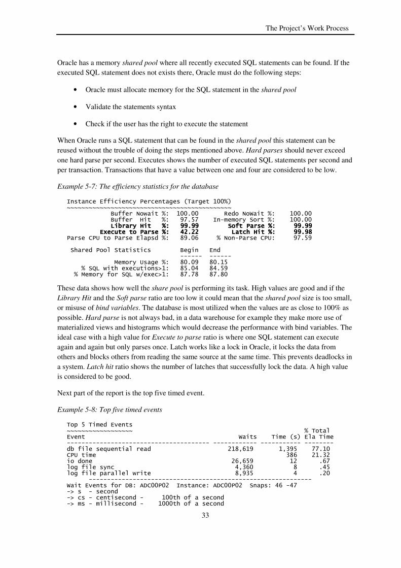
33
The Project’s Work Process
Oracle has a memory shared pool where all recently executed SQL statements can be found. If the executed SQL statement does not exists there, Oracle must do the following steps:
• Oracle must allocate memory for the SQL statement in the shared pool
• Validate the statements syntax
• Check if the user has the right to execute the statement
When Oracle runs a SQL statement that can be found in the shared pool this statement can be reused without the trouble of doing the steps mentioned above. Hard parses should never exceed one hard parse per second. Executes shows the number of executed SQL statements per second and per transaction. Transactions that have a value between one and four are considered to be low.
Example 5-7: The efficiency statistics for the database
Instance Efficiency Percentages (Target 100%) ~~~~~~~~~~~~~~~~~~~~~~~~~~~~~~~~~~~~~~~~~~~~~ Buffer Nowait %: 100.00 Redo NoWait %: 100.00 Buffer Hit %: 97.57 In-memory Sort %: 100.00 Library Hit %: 99.99 Soft Parse %: 99.99Library Hit %: 99.99 Soft Parse %: 99.99Library Hit %: 99.99 Soft Parse %: 99.99Library Hit %: 99.99 Soft Parse %: 99.99 Execute to Parse %: 42.22 Latch Hit %: 99.98Execute to Parse %: 42.22 Latch Hit %: 99.98Execute to Parse %: 42.22 Latch Hit %: 99.98Execute to Parse %: 42.22 Latch Hit %: 99.98 Parse CPU to Parse Elapsd %: 89.06 % Non-Parse CPU: 97.59 Shared Pool Statistics Begin End ------ ------ Memory Usage %: 80.09 80.15 % SQL with executions>1: 85.04 84.59 % Memory for SQL w/exec>1: 87.78 87.80
These data shows how well the share pool is performing its task. High values are good and if the Library Hit and the Soft parse ratio are too low it could mean that the shared pool size is too small, or misuse of bind variables. The database is most utilized when the values are as close to 100% as possible. Hard parse is not always bad, in a data warehouse for example they make more use of materialized views and histograms which would decrease the performance with bind variables. The ideal case with a high value for Execute to parse ratio is where one SQL statement can execute again and again but only parses once. Latch works like a lock in Oracle, it locks the data from others and blocks others from reading the same source at the same time. This prevents deadlocks in a system. Latch hit ratio shows the number of latches that successfully lock the data. A high value is considered to be good.
Next part of the report is the top five timed event.
Example 5-8: Top five timed events
Top 5 Timed Events ~~~~~~~~~~~~~~~~~~ % Total Event Waits Time (s) Ela Time --------------------------------------- ------------ ----------- -------- db file sequential read 218,619 1,395 77.10 CPU time 386 21.32 io done 26,659 12 .67 log file sync 4,360 8 .45 log file parallel write 8,935 4 .20 ------------------------------------------------------------- Wait Events for DB: ADC00P02 Instance: ADC00P02 Snaps: 46 -47 -> s - second -> cs - centisecond - 100th of a second -> ms - millisecond - 1000th of a second

34
The Project’s Work Process
The db file sequential read event as mentioned in chapter four is a wait event that the process is reading from a buffer and waiting for an I/O call to be returned. To tune this event try to change the value in PGA_AGGREGATE_TARGET. This parameter controls the amount of memory for the database to do sorting and hash join operations (page 11) [15]. The CPU time event shows that the database was doing CPU related work. If this event is at the top, CPU might be the bottleneck of the problem.
The overall results from the Statspack are good and there is no indication of any bad hard parses or any bad values in the efficiency statistics. Some SQL statements were investigated but no major changes have been made4.
Measuring the results from the Statspack with queueing theory can roughly estimate the report’s result for our system. Input the data into the queueing theory tool will give an idea to, if the system was processing or queueing for jobs. We use the value from example 5-6 in the excel tool in appendix A [3] to calculate the stress on the system, for the result see picture 5-3. The number of executes is 286.27, it was input to cell B7. The number of parses was input to cell B22. The maximum response time rmax was set to 0.01 second in cell B6. The result with theses parameter set showed that, 80.87% of all the SQL statements would be processed within 0.01 seconds per statement.
4 To see all the Statspack reports send an email to [email protected] to get the reports.

35
Performance tests’ results
Picture 5-3: The estimated calculation of the Statspack report
If the average service rate is increased to the double µ will be 330.8 SQL statements per seconds i.e. the system will process the jobs with double speed. Calculating it further with the new µ value rmax will be 96.3441% and this is valuable information before doing the actual work. The expected performance gain will be approxiamtely 16% of response time if a performance optimization is done. This is a good clue to if any more time should be spent on improving with the current conditions.
6 Performance tests’ results
The test results are divided into three parts. The first part shows the performance test results and a more detail specific description about each test. First parts test results were not planned in detail. The configurations setup was chosen mostly because of the Singl.eView documentations. This resulted into a few problems later with the bill-runs e.g. running with too many streams or spawning too many child processes and caused a bill-run failure. The first part of the tests indicated the test machines resource limit. The second part of the performance tests was to try the server

36
Performance tests’ results
configuration test setup which was more similar to the production machine. In these tests the input size has been decreased and all the configuration setup values have been lowered to a fairly stable level. During these tests some function improvements were also implemented and tested. The third part was to try the same configuration settings from part two with a larger number of customers. This will give a more reliable proof of the second part’s tests.
6.1 Part one: Performance tests’ with around 5000 customers
Tests 1-5 are the baseline with normal setting for the processes and can be up to a maximum twelve streams in Singl.eView with default settings. But my experiments were made with ten streams because of the IGP step which can only handle a load 1.2 times the number of CPUs. Streams are the number of bill-run instances that are running simultaneously. Default server settings have three of each type RGP, BGP and IGP. Later discoveries showed that the test machine could only use up to six streams in a bill-run, because there were only three RGP, BGP and IGP servers present.
Picture 6-1 shows that Denmark business two (DB2) spent more of the time in the RGP process compared to all the tested bill cycles. At that time the company still had unnessessary logics and calculations for the danish bill cycles such as tariffs. The actual time that a cycle has spent measured in hours is shown in picture 6-1. This shows that DB2 spent only 20.4 minutes (0.34 hours) in the RGP step but remember that the result was already divided into ten streams. The overall time for the danish bill cycles takes normally more time than the swedish cycles because due to unnecessary tariffs on the products. A number of these tariffis were removed later by the company to improve the performance.
Picture 6-1: Chart showing the actuall time spent in RGP’s mode calculated in hours
Looking at picture 6-1 we can see that SB4 is almost invisible in the chart. Table 5-1 and 5-3 listed that Sweden business four has only one customer and the size difference between the cycles is large. That is the reason for SB4 to almost look invisible in the chart. Each cycle is calculated with ten streams but SB4 with one customer can not divide any more customer by itself and the values are also ten times lesser than with other cycles while the rest of the streams was idle.The bill-run for SB4 was running with ten streams due to a missunderstanding in how stream works.
A recalculated chart where the SB4 cycle is not divided by ten see picture 6-2.
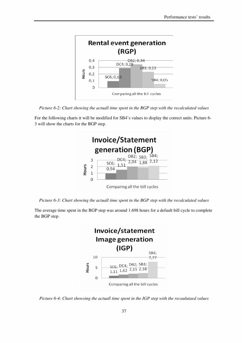
37
Performance tests’ results
Picture 6-2: Chart showing the actuall time spent in the RGP step with the recalculated values
For the following charts it will be modified for SB4’s values to display the correct units. Picture 6-3 will show the charts for the BGP step.
Picture 6-3: Chart showing the actuall time spent in the BGP step with the recalculated values
The average time spent in the BGP step was around 1.698 hours for a default bill cycle to complete the BGP step.
Picture 6-4: Chart showsing the actuall time spent in the IGP step with the recaulutaed values
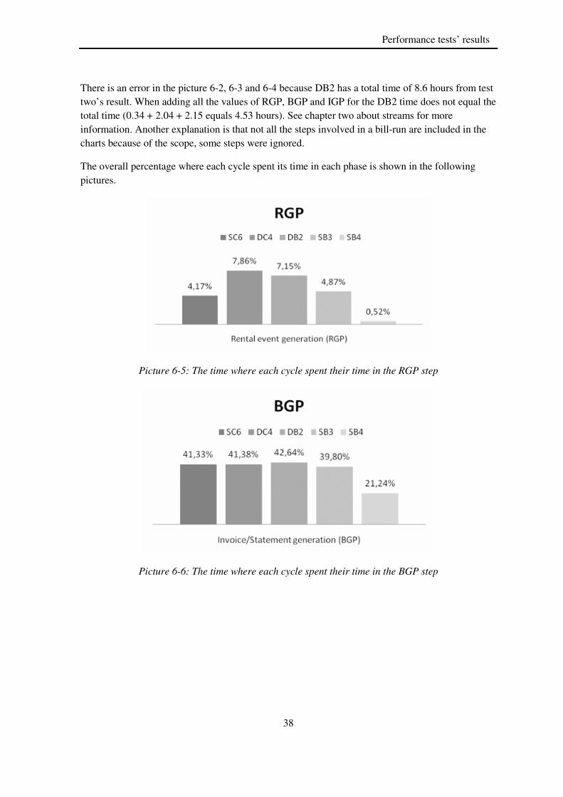
38
Performance tests’ results
There is an error in the picture 6-2, 6-3 and 6-4 because DB2 has a total time of 8.6 hours from test two’s result. When adding all the values of RGP, BGP and IGP for the DB2 time does not equal the total time (0.34 + 2.04 + 2.15 equals 4.53 hours). See chapter two about streams for more information. Another explanation is that not all the steps involved in a bill-run are included in the charts because of the scope, some steps were ignored.
The overall percentage where each cycle spent its time in each phase is shown in the following pictures.
Picture 6-5: The time where each cycle spent their time in the RGP step
Picture 6-6: The time where each cycle spent their time in the BGP step

39
Performance tests’ results
Picture 6-7: The time where each cycle spent their time in the IGP step
Test 6 was the first test with multiprocessing on the BGP configuration on a special cycle SB4. This test used twelve processes by multiplying node child processes with service child processes. Since SB4 only had one customer using two child processes would not give any benefit to the billing process in this case. This was one of the mistakes during the test experiment.
Test 8 was running from the beginning to the end of the BGP step. This run was done with eight service child processes and is equal to the number of CPUs on the server and it is the recommended settings when using multiprocessing according to [4]. With this setting the BGP step gained 36 minutes in total for SB4. In the second and third performance tests’ this setting turns out to be incorrect because of available server processes of RGP, BGP and IGP.
Picture 6-8: Improved BGP step with multiprocessing settings
Test 7 investigates if there was any possible gain by using the event child processes, but used too many processes resulted in a memory overload. An observation by using UNIX top command showed that each child process used large amount of memory and was running on full CPU utilization. Checking the log files there showed no indication of any processes that has been crashed since no new core dump files was found. A core dump file generates when a crash has been

40
Performance tests’ results
occurred during a bill-run. The process was supposed to run from the start to the end of the BGP stage. No performance gain was found and the bill-run was manually stopped.
Test 9 main purpose was to investigate if there are any gains by using the maximum number of available SCP. This was also tested with one stream to see if there was any difference in using ten streams. By checking the log files the process crashed with a core dump file and resulted to insufficient with memory. But theoretically this should be possible according to Intec [4]. In the third part of the performance tests showed that the maximum SCP should be three for the test machine.
Test 10 was to add more IGP processes by changing the IGP configuration item. This proved that the IGP step was faster than using batch streaming but still using a BGP configuration was faster in overall time. A hypothesis, to use more max child processes in IGP configuration, could give better performance and should be used on a bill cycle that spends most of their time in IGP phase. In second and third part of the performance tests showed that this parameter could improve the performance almost as much as with BGP server configuration. This test failed because too many processes were spawned.
Test 11 and 12 investigated in spawning more different BGP processes with multiprocessing. This was done by dividing the SB3 customers into two groups. One group had less than four services and the second group had four services or more. The first group was processed using the normal BGP1 configuration and the second group was processed by BGP2 configuration. The configuration file looks very similar to BGP1 default setting, except that two parameters were changed on line five and six for NCP and SCP child processes in BGP2 found in appendix C file C-2. Changing the setting will spawn more BGP processes with the following command.
cfg -f /sv/sv_pro2/work/xwuhmin/bgp.cfg
The bgp.cfg file is for example file C-2 in appendix C. The ubbconfig file is the configuration file for all the different tuxedo servers e.g. it contains the number of servers to spawn see example 5-2 from chapter five for a sample of the file that defines the number of trebgp servers to spawn. Using the new updated ubbconfig file will spawn three default trebgp servers using the BGP1 configuration and three trebgp servers using the BGP2 configuration. The eleventh test took very long time and the operation was aborted because the test took longer time to run than with the default setting. The next test was very time consuming but managed to finish the given task with no performance gained. This is also a good example when too many processes can cause a slow bill-run.
Test 13 was to measure if the batch size would affect the performance with same settings as the previous test. Lowering the batch size made the bill-run to stay much longer in the RGP step than in a normal run and this was aborted. Again too many processes were used and this bill-run was running out of resources early in the beginning which was the main reason for the slow bill-run.
Test 14 purpose was to see if the test machine could run a bill-run with many more server processes. The recommendation is to run the RGP, BGP and IGP setting equal to the number of CPUs. The test machine could not achieve the recommended settings, and the BGP child processes has been identified with insufficient with memory by checking the log files for errors.

41
Performance tests’ results
Test 15 was to analyze if another business cycle would benefit from the BGP setting by changing service and customer node. The main reason that this test failed was same as the previous test because of insufficient of resources. No performance gain was found.
Test 16 used the same settings on most parameters except on spawning three extra standard BGP processes. This should speed the process up if the BGP process does not exceed the eight CPU recommended settings. Adding extra BGP processes does not provide better performance on DB2 because the extra BGP servers were already exceeding the stable resource conditions.
Test 17 tested with smaller batch size and default server settings. The batch size was chosen based on the production machine’s setting. No improvement was found and there were some memory issues and problems with BGP child processes. The default server setting was too inappropriate with ten streams. A smaller batch size would increase the stress on the BGP child processes to consume more resources and increase the chance for a crash. An opposite case where the batch size was increased showed that the bill-run could complete with minor problem during the third performance test, see test 11 and 19 in table 5-8.
6.1.1 Summary for Part One
The following section shows charts with settings’ comparison of all the tests for different bill cycles.
Picture 6-9: Bill-run statistics for SB3 cycle
Picture 6-9 and 6-10 displays that all server- and multiserver-configurations did not perform better than the standard default bill-run. In most cases it was because of the bad settings that was used during the part one’s performance tests.

42
Performance tests’ results
Picture 6-10: DB2’s test result
In the next chart picture 6-11 shows one small improvement for the SB4 bill cycle. This improvement equals to almost 5% of performance gain.
Picture 6-11: SB4’s test result, * failed bill-run, ** testing to the BGP phase only
The rest of the bill cycles such as DC4 and SC6 had no other comparison except for the default test results that were recorded.
6.2 Part two: Results from the 100 customers cycles
Part two’s tests can be grouped into two groups where the first group was tested with eight streams while the second group was tested with three streams. The first group had 15 tests and the second group 14 tests. The tests were conducted with four cycles: DB2 (Denmark Business 2), DC4 (Denmark Consumer 4), SB3 (Sweden Business 3) and SC6 (Sweden Consumer 6). In all these tests a batch size of ten was used and a different server configuration setup was used.
The first four tests in group one were conducted with a default server configuration i.e. three of each RGP (Rental Generation Process), BGP (Bill Generation Process) and IGP (Invoice Generation Process). Same default settings as the previous performance test from the server configuration setup. All the function tests were performed with default settings from test 1-11 in table 5-6. Test 1-4 were to setup a base time for the coming tests. Tests 5-11 are the function tests. Each function change was tested with a different cycle each time to measure the performance. For

43
Performance tests’ results
most function improvements most of the changes gave a better result except for test 10. That test was testing these two functions fH3G_NUC_RecurringChgElig& and fHi3G_NUC_CampaignRecurringChgElig& on DC4. This test took 3.2 minutes longer than the baseline tests i.e. test 3. A normal default test for DC4 took 13.1 minutes. After this test these function were rolled back to its previous codes and was never tested on the other bill cycles. Testing other cycles was on a higher priority. The implemented functions gave a little performance gain the best function improvement gave 4.1 minutes of improved result of almost 32%. The average function tests gave very little performance gain shown in table 5-6. A further analysis on the server configuration setup gave at least 30% gain from the IGP tests. More time was spent in analyzing different configuration setup to increase the performance. Tests 12-15 were to measuring if all the bill cycles would benefit from the new IGP settings. These tests were done with eight MCP (Max Child Processes) in the IGP server configuration setup. Because the IGP test that was done from part one was also conducted with a mixed setup of BGP and IGP this might have cause some performance difference. Test 13 showed promising results with a gain of 32% with increased performance even with all the active function improvement. A further study for the IGP settings was made and that are the tests in group two.
In group two before the start of the tests for the baseline tests some unnecessary discount tariffs were removed from the system. In group two’s test the number of streams was changed from eight to three parallel streams. A baseline time was set and can be found in table 5-7. The IGP tests are listed from test number 5-8. An IGP test with three MCP was made for all the test cycles. This parameter is suitable for all cycle because there are no specific limitations. Each of these tests showed a major improvement when compared to the baseline test. SB3 gained most with this setting with 62% of improvement. For the BGP tests the SCP (Service Child Processes) parameter was analyzed most. This parameter is most suited for cycles with many cycles like SB4 in part one. An analyze DB2 cycle had most services per customers among the cycle see table 5-2 and test 9 was to measure the improvement. This test had a gain of 67% of improvement compared to the base time test. SB3 had 230 services and that is 60 services difference with DB2. Testing the same settings but for SB3 did not have the same effect. This test ended with only a very small performance gain of 1.7 minutes that is 6.6% gain. Another test with the Danish consumer cycle was also conducted and the result was almost the same as the baseline test with the same setting.
Test number nine to ten were to analyze if there are any performance gain when using two different setting simultaneously: three BGP SCP setting and three IGP MCP setting was used together. This setup was tested in part one before but not with this few streams. Using SB3 cycle did not improve the performance much compared to the base time. But same setting on DC4 gave the best gain for this cycle. A total gain of 44% in response time. One test with BGP NCP (Node Child Processes) parameter was tested but failed with a core dump and no other tests were performed.
6.2.1 Summary for part two
Reading from the charts SB3 was fastest to complete a bill-run with the IGP settings by changing the MAX_CHILD_PROCESSES parameter.
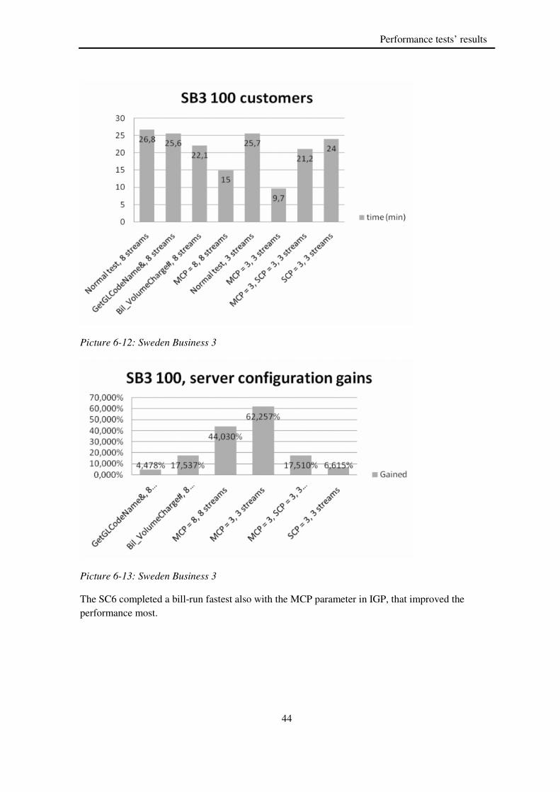
44
Performance tests’ results
Picture 6-12: Sweden Business 3
Picture 6-13: Sweden Business 3
The SC6 completed a bill-run fastest also with the MCP parameter in IGP, that improved the performance most.

45
Performance tests’ results
Picture 6-14: Sweden Consumer 6
Picture 6-15: Sweden Consumer 6
DC4 cycle performed best by running both the SCP and MCP parameter set.

46
Performance tests’ results
Picture 6-16: Denmark Consumer 4
Picture 6-17: Denmark Consumer 4
DB2 cycle had the best result of improvement with 67% by changing the SCP parameter.
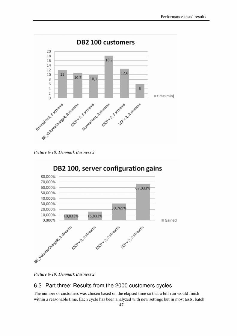
47
Performance tests’ results
Picture 6-18: Denmark Business 2
Picture 6-19: Denmark Business 2
6.3 Part three: Results from the 2000 customers cycles
The number of customers was chosen based on the elapsed time so that a bill-run would finish within a reasonable time. Each cycle has been analyzed with new settings but in most tests, batch

48
Performance tests’ results
size was set to 50 and three streams were always used. Each test is always compared to the baseline test. The SB3 cycle had a total of eight performance tests where one of them was a baseline test. Test 10 and 11 showed the resource limit of the test machine. When too many child processes were used with a small batch size then the BGP process might crash, see chapter 8.1 about process crashes. The IGP parameter MAX_CHILD_PROCESSES was once again able to increase the performance on all the tested bill cycles. Comparing with the second test phase the IGP parameter set to 3 for the MCP setting showed a performance gain of 34%. In this performance phase, problems with the SCP parameter were found. For the cause of all the bill-run crashes, see chapter 8.1 about process crashes. The BGP parameter CUSTOMER_CHILD_PROSESSES was also tested in this part and this parameter performed better than the MCP parameter in the IGP phase with one less child process and very stable bill-runs. For the SB4 cycle it gave a 40% performance boost. Combining the CCP and MCP settings gave a performance gain of 50% with the same cycle see table 5-8. The rest of the bill cycles were also tested with the same setting and the best result was attained with the CCP and MCP combination.
The SB4 cycle’s test results did not give much performance gain but it was the same as in the first phase tests’. The performance gain was 30 min when a combination of SCP and MCP was used. This cycle only has one customer so the CCP parameter would give no increased performance and with the NCP parameter gave a very small performance gain. This might indicate that the spawned child processes were too many. In table 5-9 test 2 and 3 (SB4) showed that of the spawned child processes only one was utilized. The rest of the child processes were not created. The reason was that the system only spawns one child per customer. This parameter is not very effective for bill cycles with a large customer hierarchy. All of the BGP child processes were created successfully but most of the time was spent in the IGP phase and the largest gain should also be there.
6.3.1 Summary for Part three
Picture 6-20: Sweden Consumer 6, star means stopped bill-run

49
Performance tests’ results
Picture 6-21: Sweden Consumer 6, star means stopped bill-run
Picture 6-22: Denmark Consumer 4

50
Performance tests’ results
Picture 6-23: Denmark Consumer 4
Picture 6-24: Sweden Consumer 6
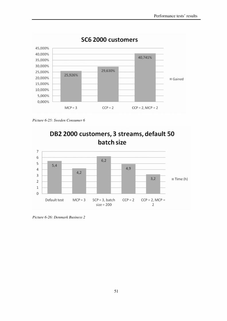
51
Performance tests’ results
Picture 6-25: Sweden Consumer 6
Picture 6-26: Denmark Business 2

52
Conclusion
Picture 6-27: Denmark Business 2
7 Conclusion
Different server configurations showed some improvements and should be tested on the production machine. Multiprocessing requires much more resources to run and can encountered more crashes than with standard settings e.g. when the wrong setting was used. To determine if multiprocessing is useful in the future smaller input to the bill-run is recommended. The settings are different from machine to machine and test result found in this project cannot be compared with the production machine’s hardware. Running more streams than available base servers e.g. RGP, BGP and IGP servers, is not recommended but can improve the performance slightly when comparing normal tests between more streamed and fewer streamed bill-runs, see picture 6-12. The best performance gain was with on a server setting with a combination of BGP and IGP settings. This result showed at least a 40% performance gain compared with the default tests with 2 000 customers on both Swedish and Danish customers. The Customer Child Processes (CCP) and the Max Child Processes (MCP) belongs to the BGP phase respectively IGP phase. These two parameters improved the performance the most on all the bill cycles with a customer count larger than one.
The abbreviations used in table 7-1 can be found in the abbreviation list at the beginning of the report.
Table 7-1: The performance gain for all the bill cycles
Server configuration
type
Parameter Customer
type
Country Gained time in
percent
BGP & IGP CCP & MCP Consumer 4 Denmark 53%
BGP & IGP CCP & MCP Business 2 Denmark 41%
BGP & IGP CCP & MCP Consumer 6 Sweden 41%
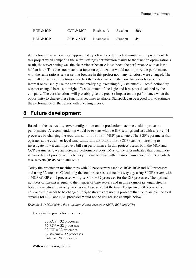
53
Future development
BGP & IGP CCP & MCP Business 3 Sweden 50%
BGP & IGP SCP & MCP Business 4 Sweden 4%
A function improvement gave approximately a few seconds to a few minutes of improvement. In this project when comparing the server setting’s optimization results to the function optimization’s result, the server setting was the clear winner because it can boost the performance with at least half an hour. This does not mean that function optimization would not improve the performance with the same ratio as server setting because in this project not many functions were changed. The internally developed functions can affect the performance on the core functions because the internal ones usually use the core functionality e.g. executing SQL statements. Core functionality was not changed because it might affect too much of the logic and it was not developed by the company. The core functions will probably give the greatest impact on the performance when the opportunity to change these functions becomes available. Statspack can be a good tool to estimate the performance on the server with queueing theory.
8 Future development
Based on the test results, server configuration on the production machine could improve the performance. A recommendation would be to start with the IGP settings and test with a few child-processes by changing the MAX_CHILD_PROCESSES (MCP) parameter. The BGP’s parameter that operates at the customer level CUSTOMER_CHILD_PROCESSES (CCP) can be interesting to investigate how it can improve a bill-run performance. In this project’s tests, both the MCP and CCP parameters gave an increased performance boost. Most of the tests indicated that using more streams did not provide with a better performance than with the maximum amount of the available base servers (RGP, BGP, and IGP).
Today the production machine runs with 32 base servers each i.e. RGP, BGP and IGP processes and using 32 streams. Calculating the total processes is done this way e.g. using 8 IGP servers with 4 MCP of IGP child processes will give 8 * 4 = 32 processes for the IGP processes. The optimal numbers of streams is equal to the number of base servers and in this example i.e. eight streams because one stream can only process one base server at the time. To spawn 8 IGP servers the ubbconfig file needs to be changed. If eight streams are used, a problem that could arise is the total streams for RGP and BGP processes would not be utilized see example below.
Example 8-1: Maximizing the utilization of base processes (RGP, BGP and IGP)
Today in the production machine:
32 RGP = 32 processes 32 BGP = 32 processes 32 IGP = 32 processes 32 streams = 32 processes Total = 128 processes
With server configuration.
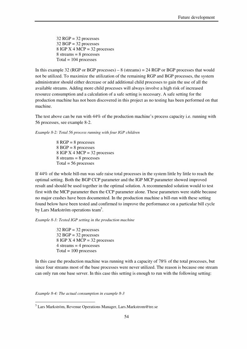
54
Future development
32 RGP = 32 processes 32 BGP = 32 processes 8 IGP X 4 MCP = 32 processes 8 streams = 8 processes
Total = 104 processes
In this example 32 (RGP or BGP processes) – 8 (streams) = 24 RGP or BGP processes that would not be utilized. To maximize the utilization of the remaining RGP and BGP processes, the system administrator should either decrease or add additional child processes to gain the use of all the available streams. Adding more child processes will always involve a high risk of increased resource consumption and a calculation of a safe setting is necessary. A safe setting for the production machine has not been discovered in this project as no testing has been performed on that machine.
The test above can be run with 44% of the production machine’s process capacity i.e. running with 56 processes, see example 8-2.
Example 8-2: Total 56 process running with four IGP children
8 RGP = 8 processes 8 BGP = 8 processes 8 IGP X 4 MCP = 32 processes 8 streams = 8 processes Total = 56 processes
If 44% of the whole bill-run was safe raise total processes in the system little by little to reach the optimal setting. Both the BGP CCP parameter and the IGP MCP parameter showed improved result and should be used together in the optimal solution. A recommended solution would to test first with the MCP parameter then the CCP parameter alone. These parameters were stable because no major crashes have been documented. In the production machine a bill-run with these setting found below have been tested and confirmed to improve the performance on a particular bill cycle by Lars Markström operations team5.
Example 8-3: Tested IGP setting in the production machine
32 RGP = 32 processes 32 BGP = 32 processes
8 IGP X 4 MCP = 32 processes 4 streams = 4 processes
Total = 100 processes
In this case the production machine was running with a capacity of 78% of the total processes, but since four streams most of the base processes were never utilized. The reason is because one stream can only run one base server. In this case this setting is enough to run with the following setting:
Example 8-4: The actual consumption in example 8-3
5 Lars Markström, Revenue Operations Manager, [email protected]

55
Future development
4 RGP = 4 processes 4 BGP = 4 processes 4 IGP X 4 MCP = 16 processes 4 streams = 4 processes
Total = 28 processes
In this case four streams were used and only four of the RGP, BGP and IGP base servers would be utilized. The rest would stay idle or waiting for an available stream. The total available process capacity compared with the default test is now 22%.
The BGP server has many options to create different levels of child processes. Due to a high risk of crashes during a bill-run when using the BGP setting this should be carefully tested as all of the crashes were associated with the BGP settings in this project. What could have caused the crashes could be resource problems or code problems in the system. As mentioned before the only stable parameter for the BGP servers is the CUSTOMER_CHILD_PROCESSES (CCP) parameter because no crashes were found when it was used.
The IGP step can also be improved with a software upgrade for Singl.eView version 7.0 according to Paul Velenik6.
8.1 How to approach the production machine
This section will provide some guidelines on how to approach the production machine with server settings. For the IGP phase example 8-4 was the setting that has been tested on the production machine. If child processes is going to be used on the production machine, a first approach is to try with a smaller input size than with the whole bill cycles. Creating smaller database tables of the bill cycles can reduce the test time and more time can be focused on finding a more stable configuration setting.
1. Create a small table from an existing table.
2. Document the solutions.
3. Run a baseline test i.e. a bill-run with default setting, to compare the next result with the baseline.
4. Calculate the required processes for this bill-run. The resource consumption should stay within the available resource limit (120 processes) for the production machine. 20% of the process capacity when using child processes is known to be stable.
5. Change the server setting to spawn the calculated processes described in example 5-1.
6. Analyze how the IGP child processes can affect the bill-run7.
7. Analyze how the BGP child processes can affect the bill-run.
6 Paul Velenik, a developer at the billing department, [email protected]
7 It is important to remember that child processes can consume more memory than a default bill-run, which means that 120 processes would not equal 120 child processes in memory consumption.

56
Future development
8. Combine the two settings if possible when positive result was obtained from steps 6 and 7.
9. Redo step one with more customers or increase the process capacity until the target ratio has been reached.
8.2 Possible problems during a bill-run
All the bill-runs did not successfully complete its task. In this project a few common problems have been uncovered. When running a server configuration, more processes will be spawned by the Tuxedo system. Which processes to spawn are based on the ubbconfig file and the server configuration items in Singl.eView. When changing the BGP setting like in example 5-1, more child processes will be spawned. Sometimes these processes needs to be terminated manually e.g. when changing from a child process setting to a default setting. The BGP children can remain after a changed setting (usually they will terminate automatically when the bill-run is done, but the system will always keep BGP child processes equal to the number of BGP servers). Use the ps UNIX command to see if there are any child processes in the background.
$ ps –alef | grep bgp_child_process
Another useful UNIX command is top. This command will show the most resource consuming processes at the top. If more processes are available they will be showed in the first page to toggle the next page press the j key to jump forward in the list and k key to jump backwards. The flag –dx followed with a number x, will refresh the first page x times. The –sy flag followed with a number y will refresh the current list every y second.
$ top –d5 –s1
When running a default bill-run and using the ps command, no child processes should be in the system e.g. bgp_child_process and igp_child. These processes should only exist when a server configuration is used, because child processes can lead to other problems during a bill-run. The symptoms can be described in the following way:
• Locked customers
• Process crash
• Slow bill-run
• Insufficient with memory
• A previous stopped bill-run running with child processes
The solution is to terminate all the Tuxedo processes with a billing_stop command and terminate the child processes by using the UNIX kill command. The ps command can find the process number for the kill command to terminate the correct process, when all the processes are cleared use the command below to clean all the remaining processes.
$ billing_clean sv_pro2 -r –F
The last step is to restart all the Tuxedo processes with a billing_start command.
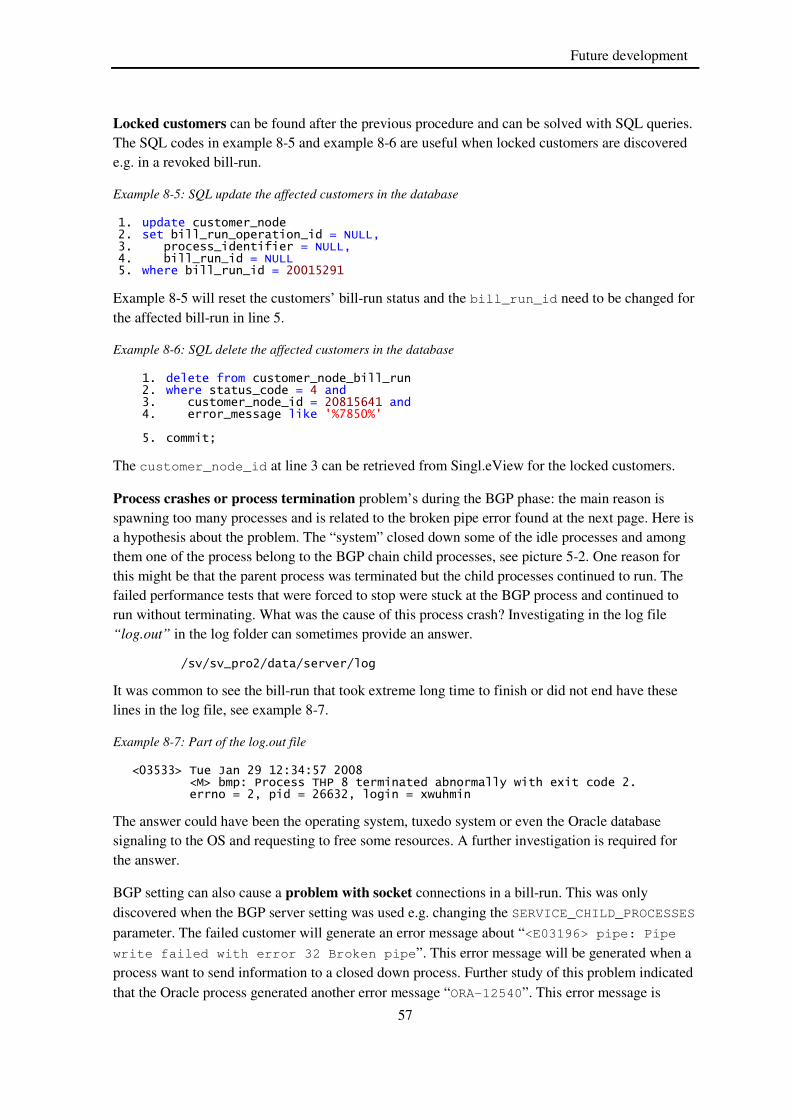
57
Future development
Locked customers can be found after the previous procedure and can be solved with SQL queries. The SQL codes in example 8-5 and example 8-6 are useful when locked customers are discovered e.g. in a revoked bill-run.
Example 8-5: SQL update the affected customers in the database
1. update customer_node 2. set bill_run_operation_id = NULL, 3. process_identifier = NULL, 4. bill_run_id = NULL 5. where bill_run_id = 20015291
Example 8-5 will reset the customers’ bill-run status and the bill_run_id need to be changed for the affected bill-run in line 5.
Example 8-6: SQL delete the affected customers in the database
1. delete from customer_node_bill_run 2. where status_code = 4 and 3. customer_node_id = 20815641 and 4. error_message like '%7850%'
5. commit;
The customer_node_id at line 3 can be retrieved from Singl.eView for the locked customers.
Process crashes or process termination problem’s during the BGP phase: the main reason is spawning too many processes and is related to the broken pipe error found at the next page. Here is a hypothesis about the problem. The “system” closed down some of the idle processes and among them one of the process belong to the BGP chain child processes, see picture 5-2. One reason for this might be that the parent process was terminated but the child processes continued to run. The failed performance tests that were forced to stop were stuck at the BGP process and continued to run without terminating. What was the cause of this process crash? Investigating in the log file “log.out” in the log folder can sometimes provide an answer.
/sv/sv_pro2/data/server/log
It was common to see the bill-run that took extreme long time to finish or did not end have these lines in the log file, see example 8-7.
Example 8-7: Part of the log.out file
<03533> Tue Jan 29 12:34:57 2008 <M> bmp: Process THP 8 terminated abnormally with exit code 2. errno = 2, pid = 26632, login = xwuhmin
The answer could have been the operating system, tuxedo system or even the Oracle database signaling to the OS and requesting to free some resources. A further investigation is required for the answer.
BGP setting can also cause a problem with socket connections in a bill-run. This was only discovered when the BGP server setting was used e.g. changing the SERVICE_CHILD_PROCESSES parameter. The failed customer will generate an error message about “<E03196> pipe: Pipe write failed with error 32 Broken pipe”. This error message will be generated when a process want to send information to a closed down process. Further study of this problem indicated that the Oracle process generated another error message “ORA-12540”. This error message is
58
Discussion
generated when too many processes are running simultaneously [16]. A suggested solution: calculate the number of spawned child processes and lower the number for the next run8.
Slow bill-runs can indicate that wrong server setting has been used if any settings were changed from the beginning. In many tests where the wrong setting was used i.e. spawning too many child processes made the bill-run finish slower than the default settings or in the worst case caused a process to terminate to early. Most test’s from the first test phase and ten and eleven in phase two in chapters five are some good examples. The cause of this problem was miscalculation of how many child processes that the machine can handle. This was the main reason for most of the bill-run failures this was discovered quite late in the project. For more information about spawned processes see chapter 5.2.
Problem with getstats. Getstats did not log all the functions that were used in a bill-run. Many BGP related settings did not show any statistics for the functions. It is unclear why this problem happens. Possible solution could be to increase the BGP statistic cache size found on line 19 in file 13-1 or maybe running server configuration is not supported by getstats. According to Adam Tong9 it could be a bug.
9 Discussion
What does the company benefit from doing more configuration tests?
Main positives factors
• A configuration setup is easy to change • Can be controlled by scripts • Can be tested unmanned by using the schedules in Singl.eView (during) night time • Performance gain for similar bill cycles • Fairly easy to get the statistics
Main negative factors
• It is very time consuming to perform • No sign of how long these test need to be done, a month or a year • Resource demanding • Hard to predict the amount of performance gain • Big difference between the production- and test-machine’s hardware setup, which means
there is a risk that there could be a memory issue involved
What can affect the configuration tests?
8 Note, when changing the number of processes other child processes might be active. Terminate these before restarting the server.
9 Adam Tong, Billing developer, [email protected]
59
Discussion
1. The available resources, because each child node that a stream creates can scale to a massive number of other new child processes when setup is incorrect.
2. The customer’s structure has an impact on how fast the bill-run can be completed e.g. the number of customers, services and events can affect the results.
3. Different machine hardware is also a very important point to consider. 4. The results found from the test machine do not have to resemble the production machine’s test
result. The consumer test cycles that were used in this project only represent less than 2% of the entire consumer cycles, while for the business cycles they represent 5% for SB3 and 13% for DB2.
Which hardware should be upgraded?
This is a very expensive last resort of investment to boost the performance. Same amount of investment money can be used to solve other problems in the company. Millsap 1999 (page 2) [14] uncovered a myth in his article: “MYTH: Installing a faster CPU always helps the performance”. He illustrated a problem by Neil Gunther with an Oracle system that process batch jobs from interactive users. Each job get processed by the CPU and then serviced by the hard drives. Neil calculated the performance gain with a five-times-faster CPU to predict how much faster the system can process the same amount of jobs. His example showed an increased performance of 20% in response time with a CPU upgrade. When the CPU was able to process the jobs faster, it made the competition of disc access even worse. This example shows the vulnerability of what happens when tuning the wrong bottleneck can decrease the performance. “When you add
capacity: add it to the bottleneck device” Millsap 1999 (page 3) [14].

60
Reference
Reference
[1] Cary Millsap, Jeffrey Holt. 2003. Optimizing Oracle Performance. O’Reilly Media, Inc. 978-0596005276
[2] ADC. 2004. Training Singl.eView, Convergent Billing v5.01. ADC Software Systems Ireland Limited.
[3] Jon Kleinberg. Éva Tardos. 2006. Algorithm Design, Pearson International Edition. Pearson Education, Inc. 0-321-37291-3
[4] Intec. 2004. System configuration guide for Singl.eView Convergent Billing v6.00. Intec Billing Ireland (An Intec Telecom Systems PLC Group Company).
[5] Intec. 2004. System operation guide for Singl.eView Convergent Billing v6.00. Intec Billing Ireland (An Intec Telecom Systems PLC Group Company).
[6] Intec. 2004. System Administration Guide for Singl.eView Convergent Billing v6.00. Intec Billing Ireland (An Intec Telecom Systems PLC Group Company).
[7] Microsoft Corporation. 20061101. Overview of Redundant Arrays of Inexpensive Disks
(RAID). Article ID 100110. URL: http://support.microsoft.com/kb/100110
[8] Dr. Myron Hlynka. 200606. FAQ on Queueing Theory. URL: http://www2.uwindsor.ca/~hlynka/qfaq.html
[9] Anjo Kolk, Shari Yamaguchi, Jim Viscusi. June 1999. Yet Another Performance Profiling
Method (or YAPP-Method). Oracle Corporation.
[10] Intec. 2004. Performance guide for Singl.eView Convergent Billing v6.00. Intec Billing Ireland (An Intec Telecom Systems PLC Group Company).
[11] Intec. 2004. Configurer’s Reference Guide for Singl.eView Convergent Billing v6.00 vol 3. Intec Billing Ireland (An Intec Telecom Systems PLC Group Company).
[12] Intec. 2004. Configurer’s Reference Guide for Singl.eView Convergent Billing v6.00 vol 2. Intec Billing Ireland (An Intec Telecom Systems PLC Group Company)
[13] Akadia AG. 20080107. Oracle Statspack Survival Guide. URL: http://www.akadia.com/services/ora_statspack_survival_guide.html
[14] Cary V. Millsap. June 28, 1999. Performance Management: Myths & Facts. Oracle Corporation.
[15] Guy Harrison. Quarter 4, 2006. Oracle performance tuning: a system approach. SELECT Journal.
[16] Oracle Corporation. June 2006. Oracle Database Error Messages 10g Release 2 (10.2)
B14219-01. Oracle Corporation.

61
Appendix A
Appendix A
Tools
[1] Simon Tatham. 20070429. Putty: A free Telenet/SSH client. URL:
http://www.chiark.greenend.org.uk/~sgtatham/putty/download.html
[2] Quest software. 2007. Toad for Oracle version 9.1.0.62. URL: http://www.quest.com/
[3] Ho Ming Wu. 2007. Queueing theory in excel spreadsheet. [email protected]

62
Appendix B
Appendix B
Table B-1: Top ten BGP functions for DB2 bill cycle
Functions Calls Elapsed time(s)
Avg(ms) Net(s) Net avg(ms)
InvoiceGenerate& 51 61738.97 1210567.96 61738.78 12105
64.22
fHi3G_Inv_GetSubStr
ing$
36412814 1380.00 0.04 1380.00 0.04
SQLQuery& 104435 1155.65 11.07 1155.65 11.07
fH3G_SplitString$[] 16043278 774.04 0.05 774.04 0.05
fH3G_ProductNames2I
ds$[]
4541770 659.40 0.15 659.40 0.15
fHi3G_Inv_GetSubStr
$
37203725 596.87 0.02 596.87 0.02
DerivedTableLookupB
yDatex&
6403638 436.67 0.07 436.67 0.07
fH3G_GetGLCodeName&
45257 1260.63 27.85 403.26 8.91
SQLQuery?[] 68888 358.90 5.21 358.90 5.21
biCustomerNodeFetch
Products&
5256 339.34 64.56 339.34 64.56
Table B-2: Top ten IGP functions for DB2
Functions Calls Elapsed time(s)
Avg(ms) Net(s) Net avg(ms)
SQLQuery& 47296 2327.27 49.21 2327.2
7
49.21
DerivedTableLookupByDatex
&
19953
148
850.30 0.04 850.30 0.04
fH3G_SearchMethod& 42443
54
1150.99 0.27 517.74 0.12
fHi3G_Inv_AggregateUsageD
etails&
44336
83
1294.00 0.29 498.76 0.11
fH3G_SplitString$[] 37676
81
463.52 0.12 463.52 0.12
fHi3G_Inv_GetDestTxt$ 21221
77
943.88 0.44 270.91 0.13

63
Appendix B
DerivedTableLookupByDate& 44336
83
228.98 0.05 228.98 0.05
biServiceSearch& 30940 128.65 4.16 128.65 4.16
CustomerNodeTableContents
?[]
5220 88.69 16.99 88.69 16.99
fHi3G_BMC_GetSortCode$ 44336
83
304.12 0.07 75.14 0.02
Table B-3: Top the RGP functions for DB2
Functions Calls Elapsed time(s)
Avg(ms) Net(s) Net avg(ms)
RentalGenerate& 102 17016.14 166824.8
5
11784.
71
115536.34
biServiceFetchByNa
me?[]
73379 3084.68 42.04 3084.6
8
42.04
biSQLQueryx& 44092
8
1092.26 2.48 1092.2
6
2.48
biSQLQueryRWx& 9023 522.93 57.96 522.93 57.96
fH3G_DerivedTableC
ontentsWpr?[]
47738
5
296.73 0.62 296.73 0.62
DerivedTableLookup
ByDatex&
95477
0
76.51 0.08 76.51 0.08
fH3G_NUC_Recurring
ChgElig&
46661
3
1524.84 3.27 57.31 0.12
biProductInstanceF
etchById&
9023 56.25 6.23 56.25 6.23
fH3G_SearchMethod& 47738
5
110.31 0.23 33.80 0.07
ReferenceCodeByLab
el&
44092
8
7.83 0.02 7.83 0.02
Table B-4: Top four NODB functions for DB2
Functions Calls Elapsed time(s) Avg(ms) Net(s) Net avg(ms)
CommandRunGetResults& 51 624.31 12241.33 624.31 12241.33
CommandRun& 5069 189.42 37.37 189.42 37.37
biCommandRun& 5069 189.76 37.44 0.34 0.07
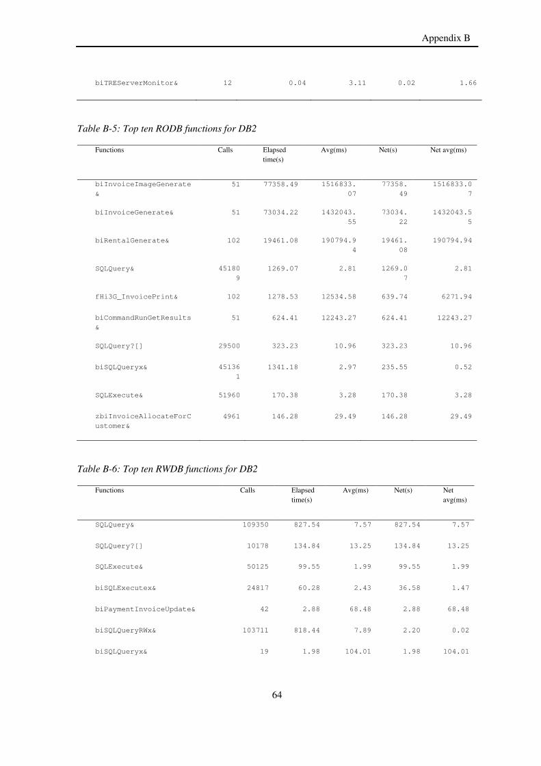
64
Appendix B
biTREServerMonitor& 12 0.04 3.11 0.02 1.66
Table B-5: Top ten RODB functions for DB2
Functions Calls Elapsed time(s)
Avg(ms) Net(s) Net avg(ms)
biInvoiceImageGenerate
&
51 77358.49 1516833.
07
77358.
49
1516833.0
7
biInvoiceGenerate& 51 73034.22 1432043.
55
73034.
22
1432043.5
5
biRentalGenerate& 102 19461.08 190794.9
4
19461.
08
190794.94
SQLQuery& 45180
9
1269.07 2.81 1269.0
7
2.81
fHi3G_InvoicePrint& 102 1278.53 12534.58 639.74 6271.94
biCommandRunGetResults
&
51 624.41 12243.27 624.41 12243.27
SQLQuery?[] 29500 323.23 10.96 323.23 10.96
biSQLQueryx& 45136
1
1341.18 2.97 235.55 0.52
SQLExecute& 51960 170.38 3.28 170.38 3.28
zbiInvoiceAllocateForC
ustomer&
4961 146.28 29.49 146.28 29.49
Table B-6: Top ten RWDB functions for DB2
Functions Calls Elapsed time(s)
Avg(ms) Net(s) Net avg(ms)
SQLQuery& 109350 827.54 7.57 827.54 7.57
SQLQuery?[] 10178 134.84 13.25 134.84 13.25
SQLExecute& 50125 99.55 1.99 99.55 1.99
biSQLExecutex& 24817 60.28 2.43 36.58 1.47
biPaymentInvoiceUpdate& 42 2.88 68.48 2.88 68.48
biSQLQueryRWx& 103711 818.44 7.89 2.20 0.02
biSQLQueryx& 19 1.98 104.01 1.98 104.01
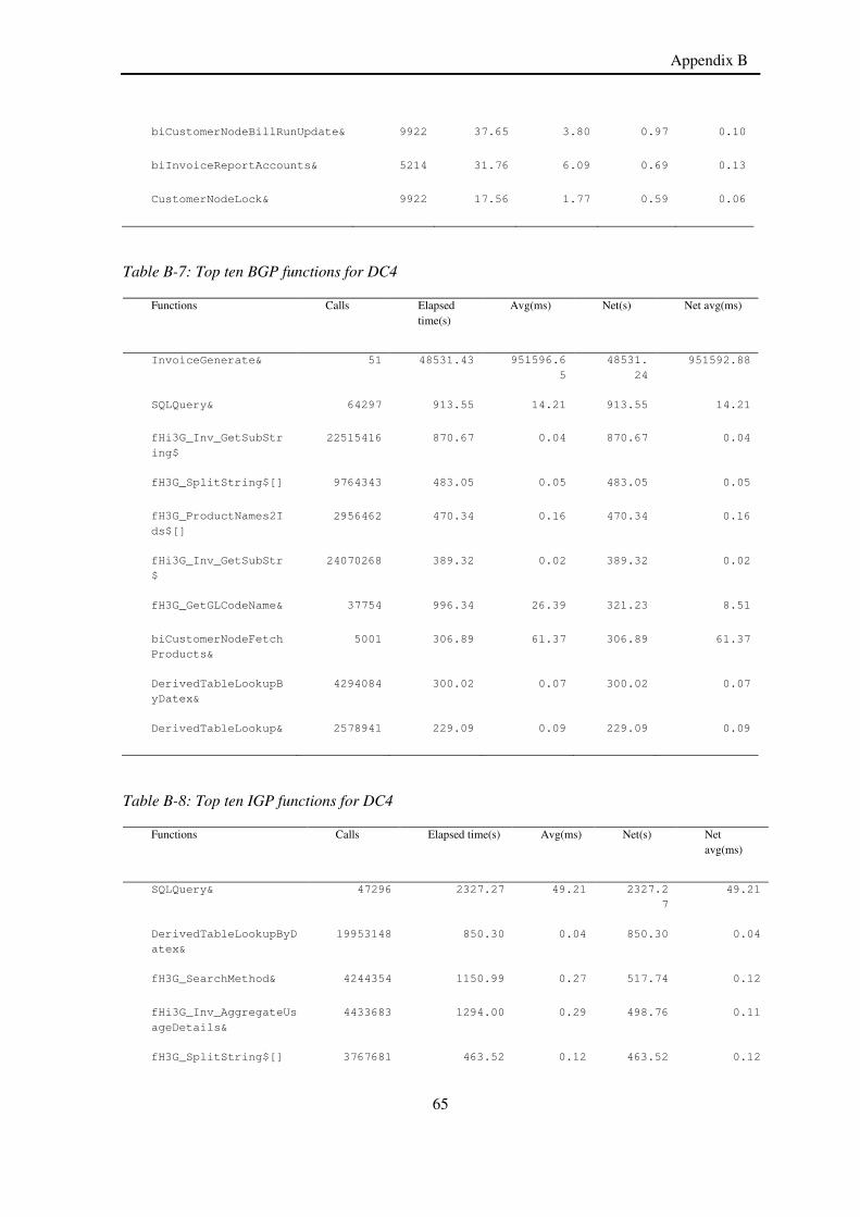
65
Appendix B
biCustomerNodeBillRunUpdate& 9922 37.65 3.80 0.97 0.10
biInvoiceReportAccounts& 5214 31.76 6.09 0.69 0.13
CustomerNodeLock& 9922 17.56 1.77 0.59 0.06
Table B-7: Top ten BGP functions for DC4
Functions Calls Elapsed time(s)
Avg(ms) Net(s) Net avg(ms)
InvoiceGenerate& 51 48531.43 951596.6
5
48531.
24
951592.88
SQLQuery& 64297 913.55 14.21 913.55 14.21
fHi3G_Inv_GetSubStr
ing$
22515416 870.67 0.04 870.67 0.04
fH3G_SplitString$[] 9764343 483.05 0.05 483.05 0.05
fH3G_ProductNames2I
ds$[]
2956462 470.34 0.16 470.34 0.16
fHi3G_Inv_GetSubStr
$
24070268 389.32 0.02 389.32 0.02
fH3G_GetGLCodeName& 37754 996.34 26.39 321.23 8.51
biCustomerNodeFetch
Products&
5001 306.89 61.37 306.89 61.37
DerivedTableLookupB
yDatex&
4294084 300.02 0.07 300.02 0.07
DerivedTableLookup& 2578941 229.09 0.09 229.09 0.09
Table B-8: Top ten IGP functions for DC4
Functions Calls Elapsed time(s) Avg(ms) Net(s) Net avg(ms)
SQLQuery& 47296 2327.27 49.21 2327.2
7
49.21
DerivedTableLookupByD
atex&
19953148 850.30 0.04 850.30 0.04
fH3G_SearchMethod& 4244354 1150.99 0.27 517.74 0.12
fHi3G_Inv_AggregateUs
ageDetails&
4433683 1294.00 0.29 498.76 0.11
fH3G_SplitString$[] 3767681 463.52 0.12 463.52 0.12

66
Appendix B
fHi3G_Inv_GetDestTxt$ 2122177 943.88 0.44 270.91 0.13
DerivedTableLookupByD
ate&
4433683 228.98 0.05 228.98 0.05
fHi3G_Inv_GetCountryT
xt$
2122177 703.34 0.33 186.70 0.09
SQLQuery?[] 10583 157.54 14.89 157.54 14.89
biSQLQueryRWx& 20868 147.33 7.06 147.33 7.06
Table B-9: Top four NODB functions for DC4
Functions Calls Elapsed time(s)
Avg(ms) Net(s) Net avg(ms)
CommandRunGetResults& 51 593.05 11628.40 593.05 11628.40
CommandRun& 5001 183.84 36.76 183.84 36.76
biCommandRun& 5001 184.19 36.83 0.35 0.07
biTREServerMonitor& 12 0.03 2.09 0.01 1.06
Table B-10: Top ten RGP functions for DC4
Functions Calls Elapsed time(s)
Avg(ms) Net(s) Net avg(ms)
RentalGenerate& 102 15004.53 147103.23 11422.85 111988.
71
biServiceFetchByName?[] 85461 1956.73 22.90 1956.73 22.90
biSQLQueryx& 344226 959.40 2.79 959.40 2.79
fH3G_DerivedTableConten
tsWpr?[]
386991 262.73 0.68 262.73 0.68
biSQLQueryRWx& 3668 228.19 62.21 228.19 62.21
DerivedTableLookupByDat
ex&
773982 64.49 0.08 64.49 0.08
fH3G_NUC_RecurringChgEl
ig&
377780 1333.16 3.53 48.24 0.13
fH3G_SearchMethod& 386991 93.05 0.24 28.56 0.07
biProductInstanceFetchB
yId&
3668 24.68 6.73 24.68 6.73

67
Appendix B
ReferenceCodeByLabel& 344226 6.62 0.02 6.62 0.02
Table B-11: Top ten RODB functions for DC4
Functions Calls Elapsed time(s)
Avg(ms) Net(s) Net avg(ms)
biInvoiceImageG
enerate&
51 58339.04 1143902.7
8
58339.04 1143902.78
biInvoiceGenera
te&
51 54194.64 1062639.9
3
54194.64 1062639.93
biRentalGenerat
e&
102 16125.45 158092.60 16125.45 158092.60
SQLQuery& 354543 1591.44 4.49 1591.44 4.49
fHi3G_InvoicePr
int&
102 1217.85 11939.73 609.28 5973.35
biCommandRunGet
Results&
51 593.15 11630.44 593.15 11630.44
SQLQuery?[] 20859 197.63 9.47 197.63 9.47
biSQLQueryx& 354433 977.74 2.76 157.77 0.45
zbiInvoiceAlloc
ateForCustomer&
5001 133.18 26.63 133.18 26.63
biCustomerNodeF
etchById&
10006 95.42 9.54 95.42 9.54
Table B-12: Top five RWDB functions for DC4
Functions Calls Elapsed time(s)
Avg(ms) Net(s) Net avg(ms)
SQLQuery& 66832 402.89 6.03 402.89 6.03
SQLQuery?[] 10002 116.74 11.67 116.74 11.67
SQLExecute& 50010 94.76 1.89 94.76 1.89
biSQLExecutex
&
25005 64.27 2.57 39.60 1.58
biPaymentInvo
iceUpdate&
66 4.14 62.78 4.14 62.78

68
Appendix B
Table B-13: Top ten BGP functions for SB3
Functions Calls Elapsed time(s) Avg(ms) Net(s) Net avg(ms)
InvoiceGenerate
&
42 61254.39 1458437.
80
61253.
77
1458423.1
6
fHi3G_Inv_GetSu
bString$
39084714 1602.50 0.04 1602.5
0
0.04
fH3G_SplitStrin
g$[]
19854203 1244.01 0.06 1244.0
1
0.06
SQLQuery& 71622 961.59 13.43 961.59 13.43
fHi3G_Inv_GetSu
bStr$
27761983 443.82 0.02 443.82 0.02
biCustomerNodeF
etchProducts&
4181 396.41 94.81 396.41 94.81
SQLQuery?[] 48392 365.87 7.56 365.87 7.56
DerivedTableLoo
kupByDatex&
4471764 311.34 0.07 311.34 0.07
DerivedTableLoo
kup&
2687001 236.87 0.09 236.87 0.09
fH3G_GetGLCodeN
ame&
33698 541.54 16.07 168.55 5.00
Table B-14: Top ten IGP functions for SB3
Functions Calls Elapsed time(s) Avg(ms) Net(s) Net avg(ms)
SQLQuery& 35850 2816.60 78.57 2816.6
0
78.57
DerivedTableLookupB
yDatex&
19124860 834.82 0.04 834.82 0.04
fH3G_SearchMethod& 4418008 1153.63 0.26 530.11 0.12
fHi3G_Inv_Aggregate
UsageDetails&
3332034 1072.85 0.32 423.31 0.13
fH3G_SplitString$[] 3248077 373.47 0.11 373.47 0.11
fHi3G_Inv_GetDestTx
t$
2209004 988.20 0.45 286.14 0.13
fHi3G_Inv_GetCountr
yTxt$
2209004 725.31 0.33 233.01 0.11
SQLQuery?[] 8431 213.33 25.30 213.33 25.30

69
Appendix B
DerivedTableLookupB
yDate&
3332034 184.97 0.06 184.97 0.06
DerivedTableLookup& 2552633 117.29 0.05 117.29 0.05
Table B-15: Top ten NODB functions for SB3
Functions Calls Elapsed time(s)
Avg(ms) Net(s) Net avg(ms)
CommandRunGetResults& 42 503.48 11987.58 503.48 11987.58
CommandRun& 4070 158.80 39.02 158.80 39.02
biCommandRun& 4070 159.08 39.09 0.28 0.07
biTREServerMonitor& 12 0.09 7.09 0.07 6.04
Table B-16: Top seven RGP functions for SB3
Functions Calls Elapsed time(s) Avg(ms) Net(s) Net avg(ms)
RentalGenerate& 78 14548.41 186518.11 12095.
37
155068.88
biSQLQueryRWx& 15395 884.96 57.48 884.96 57.48
biSQLQueryx& 246001 803.30 3.27 803.30 3.27
biServiceFetchB
yName?[]
5036 406.17 80.65 406.17 80.65
fH3G_DerivedTab
leContentsWpr?[
]
246127 164.44 0.67 164.44 0.67
biProductInstan
ceFetchById&
15395 95.64 6.21 95.64 6.21
DerivedTableLoo
kupByDatex&
492254 40.77 0.08 40.77 0.08
Table B-17: Top ten RODB functions for SB3
Functions Calls Elapsed time(s) Avg(ms) Net(s) Net avg(ms)
biInvoiceImageG
enerate&
42 85545.45 2036796.3
3
85545
.45
2036796.33

70
Appendix B
biInvoiceGenera
te&
42 67459.91 1606188.4
3
67459
.91
1606188.43
biRentalGenerat
e&
78 14548.70 186521.77 14548
.70
186521.77
SQLQuery& 255394 1125.26 4.41 1125.
26
4.41
fHi3G_InvoicePr
int&
84 1031.27 12277.05 515.9
1
6141.76
biCommandRunGet
Results&
42 503.70 11992.96 503.7
0
11992.96
SQLQuery?[] 17296 476.67 27.56 476.6
7
27.56
biSQLQueryx& 254773 1437.70 5.64 425.8
2
1.67
zbiInvoiceAlloc
ateForCustomer&
4058 335.77 82.74 335.7
7
82.74
SQLExecute& 42056 141.36 3.36 141.3
6
3.36
Table B-18: Top five RWDB functions for SB3
Functions Calls Elapsed time(s)
Avg(ms) Net(s) Net avg(ms)
SQLQuery& 68232 1029.27 15.08 1029.27 15.08
SQLQuery?[] 8196 312.30 38.10 312.30 38.10
SQLExecute& 40743 77.20 1.89 77.20 1.89
biSQLExecutex& 20302 48.63 2.40 29.74 1.46
biBillRunSummary?{} 2 9.80 4899.73 9.80 4899.73
Table B-19: Top ten BGP functions for SB4
Functions Calls Elapsed time(s) Avg(ms) Net(s) Net avg(ms)
InvoiceGenerate
&
1 7643.86 7643859.
14
7643.8
0
7643803.14
fHi3G_Inv_GetSu
bString$
8983397 326.01 0.04 326.01 0.04
fH3G_SplitStrin
g$[]
3995838 227.24 0.06 227.24 0.06

71
Appendix B
fHi3G_Inv_GetSu
bStr$
8270134 128.21 0.02 128.21 0.02
DerivedTableLoo
kupByDatex&
1358687 75.98 0.06 75.98 0.06
fHi3G_Inv_Deriv
eChargeFieldsIn
f%
1364184 304.63 0.22 35.23 0.03
SQLQuery?[] 10277 32.82 3.19 32.82 3.19
DerivedTableLoo
kup&
548891 31.53 0.06 31.53 0.06
fHi3G_Inv_IsDKC
ust&
5706751 27.28 0.00 27.28 0.00
fHi3G_FM_Decode
Multiple&
1902729 36.88 0.02 22.08 0.01
Table B-20: Top ten IGP functions for SB4
Functions Calls Elapsed time(s) Avg(ms) Net(s) Net avg(ms)
DerivedTableLookupByD
atex&
2439351 107.26 0.04 107.2
6
0.04
fHi3G_Inv_AggregateUs
ageDetails&
943845 185.36 0.20 69.81 0.07
fH3G_SplitString$[] 480312 58.67 0.12 58.67 0.12
fH3G_SearchMethod& 418216 108.63 0.26 49.26 0.12
DerivedTableLookupByD
ate&
943845 47.15 0.05 47.15 0.05
SQLQuery& 2599 41.85 16.10 41.85 16.10
biServiceSearch& 5134 28.55 5.56 28.55 5.56
SQLQuery?[] 11 25.99 2362.3
3
25.99 2362.33
fHi3G_Inv_GetDestTxt$ 209108 89.22 0.43 25.50 0.12
fHi3G_Inv_GetCountryT
xt$
209108 70.23 0.34 22.04 0.11
Table B-21: Top three NODB functions for SB4
Functions Calls Elapsed time(s)
Avg(ms) Net(s) Net avg(ms)
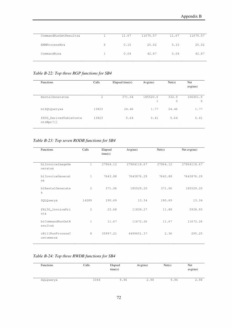
72
Appendix B
CommandRunGetResults& 1 11.67 11670.57 11.67 11670.57
ENMProcessNr& 6 0.15 25.02 0.15 25.02
CommandRun& 1 0.04 42.87 0.04 42.87
Table B-22: Top three RGP functions for SB4
Functions Calls Elapsed time(s) Avg(ms) Net(s) Net avg(ms)
RentalGenerate& 2 371.04 185520.6
1
332.9
0
166451.9
9
biSQLQueryx& 13823 24.46 1.77 24.46 1.77
fH3G_DerivedTableConte
ntsWpr?[]
13823 5.64 0.41 5.64 0.41
Table B-23: Top seven RODB functions for SB4
Functions Calls Elapsed time(s)
Avg(ms) Net(s) Net avg(ms)
biInvoiceImageGe
nerate&
1 27964.12 27964118.67 27964.12 27964118.67
biInvoiceGenerat
e&
1 7643.88 7643876.29 7643.88 7643876.29
biRentalGenerate
&
2 371.06 185529.20 371.06 185529.20
SQLQuery& 14289 190.69 13.34 190.69 13.34
fHi3G_InvoicePri
nt&
2 23.68 11838.27 11.88 5938.93
biCommandRunGetR
esults&
1 11.67 11672.26 11.67 11672.26
zBillRunProcessC
ustomers&
8 35997.21 4499651.37 2.36 295.25
Table B-24: Top three RWDB functions for SB4
Functions Calls Elapsed time(s)
Avg(ms) Net(s) Net avg(ms)
SQLQuery& 3344 9.96 2.98 9.96 2.98

73
Appendix B
biSQLQueryx& 72 2.25 31.26 2.25 31.26
ENMProcessNr& 31 1.52 49.08 1.52 49.08
Table B-25: Top ten BGP functions for SC6
Functions Calls Elapsed time(s) Avg(ms) Net(s) Net avg(ms)
InvoiceGenerate& 51 30433.81 596741.45 30433.63 596737.9
3
fHi3G_Inv_GetSub
String$
184127
04
740.93 0.04 740.93 0.04
fH3G_SplitString
$[]
103621
87
641.92 0.06 641.92 0.06
SQLQuery& 56223 634.72 11.29 634.72 11.29
biCustomerNodeFe
tchProducts&
5001 281.69 56.33 281.69 56.33
fHi3G_Inv_GetSub
Str$
140119
33
224.20 0.02 224.20 0.02
fH3G_GetGLCodeNa
me&
41077 573.35 13.96 186.67 4.54
biCommandRun& 5001 184.20 36.83 184.20 36.83
DerivedTableLook
upByDatex&
227214
0
164.76 0.07 164.76 0.07
SQLQuery?[] 29848 159.57 5.35 159.57 5.35
Table B-26: Top IGP functions for SC6
Functions Calls Elapsed time(s)
Avg(ms) Net(s) Net avg(ms)
SQLQuery& 36132 456.61 12.64 456.6
1
12.64
DerivedTableLookupByDate
x&
9057014 401.64 0.04 401.6
4
0.04
fH3G_SearchMethod& 1992496 544.80 0.27 247.8
4
0.12
fHi3G_Inv_AggregateUsage
Details&
1635365 506.97 0.31 199.5
7
0.12
fH3G_SplitString$[] 1531444 180.55 0.12 180.5
5
0.12

74
Appendix B
fHi3G_Inv_GetDestTxt$ 996248 454.01 0.46 132.9
3
0.13
fHi3G_Inv_GetCountryTxt$ 996248 341.38 0.34 99.26 0.10
biSQLQueryRWx& 20004 95.27 4.76 95.27 4.76
DerivedTableLookupByDate
&
1635365 89.87 0.05 89.87 0.05
SQLQuery?[] 10097 73.24 7.25 73.24 7.25
Table B-27: Top four NODB functions for SC6
Functions Calls Elapsed time(s)
Avg(ms) Net(s) Net avg(ms)
CommandRunGetResults& 51 542.97 10646.37 542.97 10646.37
CommandRun& 5001 176.35 35.26 176.35 35.26
biCommandRun& 5001 176.69 35.33 0.34 0.07
biTREServerMonitor& 36 0.10 2.79 0.05 1.35
Table B-28: Top eight RGP functions for SC6
Functions Calls Elapsed time(s) Avg(ms) Net(s) Net avg(ms)
RentalGenerate& 102 6365.64 62408.23 4634.80 45439.19
biSQLQueryRWx& 21260 1210.59 56.94 1210.59 56.94
biSQLQueryx& 86836 288.41 3.32 288.41 3.32
biProductInstanceF
etchById&
21260 132.21 6.22 132.21 6.22
fH3G_DerivedTableC
ontentsWpr?[]
86836 60.27 0.69 60.27 0.69
DerivedTableLookup
ByDatex&
173672 15.44 0.09 15.44 0.09
fH3G_NUC_Recurring
ChgElig&
53893 236.75 4.39 7.53 0.14
fH3G_SearchMethod& 86836 21.83 0.25 6.38 0.07

75
Appendix B
Table B-29: Top ten RODB functions for SC6
Functions Calls Elapsed time(s) Avg(ms) Net(s) Net avg(ms)
biInvoiceImag
eGenerate&
51 39830.51 780990.48 39830.51 780990.48
biInvoiceGene
rate&
51 33896.45 664636.23 33896.45 664636.23
biRentalGener
ate&
102 6932.15 67962.24 6932.15 67962.24
SQLQuery& 97829 611.57 6.25 611.57 6.25
fHi3G_Invoice
Print&
102 1115.98 10940.95 558.32 5473.77
biCommandRunG
etResults&
51 543.07 10648.42 543.07 10648.42
SQLQuery?[] 27554 205.68 7.46 205.68 7.46
zbiInvoiceAll
ocateForCusto
mer&
5001 121.32 24.26 121.32 24.26
biCustomerNod
eFetchById&
10046 88.99 8.86 88.99 8.86
biCustomerNod
eBillRunUpdat
e&
10002 74.47 7.45 74.47 7.45
Table B-30: Top seven RWDB functions for SC6
Functions Calls Elapsed time(s)
Avg(ms) Net(s) Net avg(ms)
SQLQuery& 64192 1267.36 19.74 1267.36 19.74
SQLQuery?[] 10002 106.12 10.61 106.12 10.61
SQLExecute& 50010 85.15 1.70 85.15 1.70
biSQLExecutex& 25005 60.94 2.44 37.43 1.50
biPaymentInvoiceUpdate& 73 2.84 38.86 2.84 38.86
biSQLQueryx& 60 1.85 30.84 1.85 30.84
biSQLQueryRWx& 58527 1257.35 21.48 1.18 0.02

76
Appendix B
Embedded excel spread sheet data
This functionality works only with Microsoft Word or other program that can open and edit doc files.
Table B-31: DB2 BGP function statistics (double click to edit)
Function Calls ElapsedTimeG_ElapsedPerG_ElapsedAvgElapsedMinElapsedMax
InvoiceGenerate& 51 61738,97 9,72 1210568 3418,41 2684702
fHi3G_Inv_GetSubString$36412814 61738,97 0,22 0,04 0,01 10,26
SQLQuery& 104435 1549,45 0,18 11,07 0,73 483,02
fH3G_SplitString$[]16043278 1399,54 0,12 0,05 0 7,4
fH3G_ProductNames2Ids$[]4541770 1380 0,1 0,15 0,04 11,42
fHi3G_Inv_GetSubStr$37203725 1260,63 0,09 0,02 0,01 13,76
DerivedTableLookupByDatex&6403638 1155,65 0,07 0,07 0,02 99,84
fH3G_GetGLCodeName&45257 904,63 0,2 27,85 0,04 140,32
SQLQuery?[] 68888 832,85 0,06 5,21 0,93 389,53
Table B-32: DB2 IGP function statistics
Function Calls ElapsedTimeG_ElapsedPerG_ElapsedAvgElapsedMinElapsedMax
SQLQuery& 47296 2327,27 0,37 49,21 0,81 24711,76
fHi3G_Inv_GetPackageCount&5217 1985,67 0,31 380,61 12,47 24713,13
fHi3G_Inv_AggregateUsageDetails&4433683 1294 0,2 0,29 0,06 424,54
fH3G_SearchMethod&4244354 1150,99 0,18 0,27 0,08 7,38
fHi3G_Inv_GetDestTxt$2122177 943,88 0,15 0,44 0,18 7,62
DerivedTableLookupByDatex&19953148 850,3 0,13 0,04 0,03 693,14
fHi3G_Inv_GetCountryTxt$2122177 703,34 0,11 0,33 0,19 7,43
fH3G_SplitString$[]3767681 463,52 0,07 0,12 0,01 4,29
fHi3G_BMC_GetSortCode$4433683 304,12 0,05 0,07 0,04 3,41
Table B-33: DB2 NODB function statistics
Function Calls ElapsedTimeG_ElapsedPerG_ElapsedAvgElapsedMinElapsedMax
biCommandRunGetResults&51 631,1 0,03 12374,48 1220,59 18087,05
CommandRunGetResults&51 631,09 0,03 12374,39 1220,51 18086,97
biCommandRun&5069 199,34 0,01 39,32 30,45 550,28
CommandRun& 5069 198,97 0,01 39,25 30,39 550,2
treStats?[] 12 0,06 0 4,78 0,18 36,43
biTREServerMonitor&6 0,01 0 1,45 1,38 1,63
biMonitorLog& 6 0 0 0,47 0,42 0,54
ProcessStats?{} 12 0 0 0,1 0,08 0,15
DerivedTableCacheStatistics&6 0 0 0,05 0,04 0,06
Table B-34: DB2 RGP function statistics

77
Appendix B
Function Calls ElapsedTimeG_ElapsedPerG_ElapsedAvgElapsedMinElapsedMax
biRentalGenerate&102 17101,21 1,69 167658,9 1395,4 401498
RentalGenerate& 102 17101,2 1,69 167658,8 1395,36 401497,9
biServiceFetchByName?[]73379 3195,85 0,32 43,55 0,56 2457,95
fH3G_NUC_RecurringChgElig&466613 1518,72 0,15 3,25 0,45 5668,01
biSQLQueryx&440928 1095,68 0,11 2,48 1,2 5666,96
fHi3G_RC_Eligibility&9023 600,38 0,06 66,54 56,7 1083,55
biSQLQueryRWx&9023 543,18 0,05 60,2 52,72 1077,56
fH3G_DerivedTableContentsWpr?[]477385 281,44 0,03 0,59 0,27 554,39
fH3G_SearchMethod&477385 115,3 0,01 0,24 0,12 737,12
Table B-35: DB2 RODB function statistics
Function Calls ElapsedTimeG_ElapsedPerG_ElapsedAvgElapsedMinElapsedMax
biBillRunExecute& 83 174947,9 3,22 2107806 94,44 8084547
zBillRunProcessCustomers&440 174947,5 3,22 397607,8 57,65 3976757
biBillRunInvoiceImageGenerate&51 86674,2 1,6 1699494 1590,45 3976721
biInvoiceImageGenerate&51 86674,19 1,6 1699494 1590,35 3976721
biBillRunInvoiceGenerate&51 66776,3 1,23 1309339 3549,49 3711334
biInvoiceGenerate&51 66552,85 1,23 1304958 3549,36 3711312
biRentalGenerate&102 19546,79 0,36 191635,2 1396,75 708277,3
biBillRunRentalGenerate&51 12404,89 0,23 243233,2 1555,25 708277,4
biBillRunRentalAdjustmentGenerate&51 7141,91 0,13 140037,5 1396,85 478707,5
Table B-36: DB2 RWDB function statistics
Function Calls ElapsedTimeG_ElapsedPerG_ElapsedAvgElapsedMinElapsedMax
SQLQuery& 109350 849,91 0,01 7,77 0,61 1074,44
biSQLQueryRWx&103711 840,48 0,01 8,1 0,75 1074,47
zbiInvoiceAllocateForCustomer&4961 144,39 0 29,1 1,44 2002,51
SQLQuery?[] 10178 142,46 0 14 0,7 988,89
SQLExecute& 50125 106,34 0 2,12 0,57 147,88
biSQLExecutex&24817 62,34 0 2,51 0,64 147,91
biCustomerNodeBillRunUpdate&9922 38,91 0 3,92 1,86 60,62
biInvoiceReportAccounts&5214 35,47 0 6,8 3,76 340,57
biCustomerNodeBillRunInsert&4961 28,62 0 5,77 0,93 147,08
Table B-37: DC4 BGP function statistics

78
Appendix B
Function Calls ElapsedTimeG_ElapsedPerG_ElapsedAvgElapsedMinElapsedMax
InvoiceGenerate& 51 48531,43 6,22 951596,7 4377,63 1619701
biInvoiceGenerate&51 48531,43 6,22 951596,7 4377,66 1619701
fH3G_AssignGLInfo&37754 1108,47 0,14 29,36 0,2 194,36
fHi3G_Inv_DeriveChargeFieldsInfo${}3937135 1021,11 0,13 0,26 0,05 20,59
fH3G_GetGLCodeName&37754 996,34 0,13 26,39 0,04 183,7
SQLQuery& 64297 913,55 0,12 14,21 0,82 425,94
fHi3G_Inv_GetSubString$22515416 870,67 0,11 0,04 0,01 25,55
fH3G_Bil_GetPerEventDiscounts&{}2924644 601,3 0,08 0,21 0,07 18,03
fHi3G_BIL_AssignRatedChargeFields&11784 597,29 0,08 50,69 0,24 177,2
Table B-38: DC4 IGP function statistics
Function Calls ElapsedTimeG_ElapsedPerG_ElapsedAvgElapsedMinElapsedMax
SQLQuery& 37073 1829,72 0,23 49,35 0,92 23199,69
fHi3G_Inv_GetPackageCount&5001 1586,15 0,2 317,17 13,51 23201,24
fH3G_SearchMethod&4391636 1276,48 0,16 0,29 0,08 28,15
fHi3G_Inv_GetDestTxt$2195818 1019,04 0,13 0,46 0,18 29,72
fHi3G_Inv_AggregateUsageDetails&2884291 984,35 0,13 0,34 0,06 29,66
DerivedTableLookupByDatex&19754143 861,22 0,11 0,04 0,03 26,94
fHi3G_Inv_GetCountryTxt$2195818 786,27 0,1 0,36 0,19 30,55
fH3G_SplitString$[]2643825 336,3 0,04 0,13 0,01 29,4
SQLQuery?[] 10205 258,94 0,03 25,37 0,85 6344,78
Table B-39: DC4 NODB function statistics
Function Calls ElapsedTimeG_ElapsedPerG_ElapsedAvgElapsedMinElapsedMax
CommandRunGetResults&51 593,05 0,04 11628,4 1349,92 15893,6
biCommandRunGetResults&51 593,05 0,04 11628,48 1349,99 15893,66
biCommandRun&5001 184,19 0,01 36,83 30,08 433,08
CommandRun& 5001 183,84 0,01 36,76 30 432,99
biTREServerMonitor&6 0,01 0 1,43 1,22 1,7
biMonitorLog& 6 0 0 0,47 0,4 0,53
treStats?[] 12 0 0 0,19 0,13 0,29
ProcessStats?{} 12 0 0 0,08 0,06 0,1
DerivedTableCacheStatistics&6 0 0 0,05 0,03 0,06
Table B-40: DC4 RGP function statistics

79
Appendix B
Function Calls ElapsedTimeG_ElapsedPerG_ElapsedAvgElapsedMinElapsedMax
biRentalGenerate&102 15004,54 1,92 147103,4 651,07 274728,8
RentalGenerate& 102 15004,53 1,92 147103,2 651,03 274728,7
biServiceFetchByName?[]85461 1956,73 0,25 22,9 0,57 1127,13
fH3G_NUC_RecurringChgElig&377780 1333,16 0,17 3,53 0,46 1511,41
biSQLQueryx&344226 959,4 0,12 2,79 1,21 1510,17
fH3G_DerivedTableContentsWpr?[]386991 262,73 0,03 0,68 0,27 19,06
fHi3G_RC_Eligibility&3668 253,58 0,03 69,13 55,98 670,32
biSQLQueryRWx&3668 228,19 0,03 62,21 51,87 663,61
fH3G_SearchMethod&386991 93,05 0,01 0,24 0,11 18,34
Table B-41: DC4 RODB function statistics
Function Calls ElapsedTimeG_ElapsedPerG_ElapsedAvgElapsedMinElapsedMax
biBillRunExecute& 51 130994,8 3,14 2568525 679604,3 4530873
zBillRunProcessCustomers&408 130994,5 3,14 321064,9 64,14 2600808
biBillRunInvoiceImageGenerate&51 58339,05 1,4 1143903 450589,2 2307145
biInvoiceImageGenerate&51 58339,04 1,4 1143903 450589 2307145
biBillRunInvoiceGenerate&51 54194,65 1,3 1062640 4379,41 2600764
biInvoiceGenerate&51 54194,64 1,3 1062640 4379,28 2600764
biRentalGenerate&102 16125,45 0,39 158092,6 652,5 371845,2
biBillRunRentalGenerate&51 10302,09 0,25 202001,7 2252,69 371845,4
biBillRunRentalAdjustmentGenerate&51 5823,37 0,14 114183,8 652,57 205266,5
Table B-42: DC4 RWDB functions statistics
Function Calls ElapsedTimeG_ElapsedPerG_ElapsedAvgElapsedMinElapsedMax
SQLQuery& 66832 402,89 0 6,03 0,61 659,76
biSQLQueryRWx&61226 391,74 0 6,4 0,73 659,79
zbiInvoiceAllocateForCustomer&5001 121,57 0 24,31 1,67 508,57
SQLQuery?[] 10002 116,74 0 11,67 0,78 308,77
SQLExecute& 50010 94,76 0 1,89 0,65 569,43
biSQLExecutex&25005 64,27 0 2,57 0,66 141
biCustomerNodeBillRunUpdate&10002 40,78 0 4,08 1,92 60,37
biInvoiceReportAccounts&5001 33,96 0 6,79 3,77 573,93
biCustomerNodeUnlock&10002 17,97 0 1,8 0,87 71,7
Table B-43: SB3 BGP function statistics

80
Appendix B
Function Calls ElapsedTimeG_ElapsedPerG_ElapsedAvgElapsedMinElapsedMax
InvoiceGenerate& 51 74456,44 4,39 1459930 362272,8 6130782
biInvoiceGenerate&44 37749,91 2,23 857952,4 362272,8 1200280
biInvoiceGenerateHighVolume&7 36706,58 2,17 5243797 3782087 6130782
fHi3G_Inv_GetSubString$41802189 1675,18 0,1 0,04 0,01 55,74
fH3G_SplitString$[]22611207 1415,14 0,08 0,06 0 61,28
fHi3G_Inv_DeriveChargeFieldsInfo${}5126975 1335,42 0,08 0,26 0,05 317,59
SQLQuery& 83555 1265,5 0,07 15,15 0,73 1030,55
fHi3G_Inv_GetFreeQuantity#3276293 918,52 0,05 0,28 0,23 61,66
fH3G_SplitStringPos$8403268 774,14 0,05 0,09 0,01 61,31
Table B-44: SB3 IGP function statistics
Function Direction Calls ElapsedTimeG_ElapsedPerG_ElapsedAvgElapsedMin
biInvoiceImageGenerate&IN 51 85238,16 6,7 1671337 580174,2
biSQLQueryRWx&OUT 20268 118,18 0,01 5,83 1,65
biServiceSearch&OUT 24660 102,67 0,01 4,16 1,77
biInvoiceReportAccounts&OUT 5063 63,64 0,01 12,57 6,34
biPersonFetchById&OUT 5067 51,35 0 10,13 6,43
biServiceFetchById?[]OUT 43 0,9 0 21,03 0,57
fH3G_InvoiceReportStatementAccounts&OUT 4 0,1 0 23,93 14,29
biMonitorLog&OUT 3 0 0 1,17 1,13
Table B-45: SB3 NODB function statistics
Function Calls ElapsedTimeG_ElapsedPerG_ElapsedAvgElapsedMinElapsedMax
CommandRunGetResults&51 647,06 0,03 12687,44 2930,89 25331,19
biCommandRunGetResults&51 647,06 0,03 12687,51 2930,95 25331,25
biCommandRun&4959 215,73 0,01 43,5 30,33 2580,76
CommandRun& 4959 215,38 0,01 43,43 30,26 2580,69
treStats?[] 12 0,09 0 7,34 0,13 42,07
biTREServerMonitor&6 0,01 0 1,45 1,23 1,73
biMonitorLog& 6 0 0 0,49 0,4 0,6
ProcessStats?{} 12 0 0 0,09 0,06 0,15
DerivedTableCacheStatistics&6 0 0 0,05 0,03 0,06
Table B-46: SB3 RGP function statistics

81
Appendix B
Function Calls ElapsedTimeG_ElapsedPerG_ElapsedAvgElapsedMinElapsedMax
biRentalGenerate&102 17038,27 1,34 167041,8 15935,15 652688,7
RentalGenerate& 102 17038,25 1,34 167041,7 15935,1 652688,6
fHi3G_RC_Eligibility&18414 1180,75 0,09 64,12 56,21 833,74
biSQLQueryRWx&18414 1071,09 0,08 58,17 52,34 827,95
fH3G_NUC_RecurringChgElig&266835 1041,66 0,08 3,9 0,45 200,25
biServiceFetchByName?[]26576 966,84 0,08 36,38 0,54 1950,5
biSQLQueryx&304089 922,6 0,07 3,03 1,2 80
fH3G_DerivedTableContentsWpr?[]304625 171,05 0,01 0,56 0,27 201,73
fHi3G_NUC_CampaignRecurringChgElig&37790 163,25 0,01 4,32 1,85 207,13
Table B-47: SB3 RODB function statistics
Function Calls ElapsedTimeG_ElapsedPerG_ElapsedAvgElapsedMinElapsedMax
biBillRunExecute& 80 286952,4 4,22 3586905 112,43 37098348
zBillRunProcessCustomers&437 286952 4,22 656640,6 110,31 29873186
biBillRunInvoiceGenerateHighVolume&7 126723,3 1,86 18103330 5249307 29873042
biInvoiceGenerateHighVolume&7 126723,3 1,86 18103324 5249307 29873025
biBillRunInvoiceImageGenerate&51 97844,16 1,44 1918513 580178,1 7169193
biInvoiceImageGenerate&51 97844,15 1,44 1918513 580178 7169193
biBillRunInvoiceGenerate&44 38338,57 0,56 871331,1 362274,7 1301101
biInvoiceGenerate&44 38129,39 0,56 866576,9 362274,6 1301101
biRentalGenerate&102 21300,46 0,31 208828 15936,85 1289645
Table B-48: SB3 RWDB function statistic
Function Calls ElapsedTimeG_ElapsedPerG_ElapsedAvgElapsedMinElapsedMax
SQLQuery& 82162 1241,96 0,01 15,12 0,61 825,16
biSQLQueryRWx&75460 1223,24 0,01 16,21 0,72 825,19
zbiInvoiceAllocateForCustomer&4945 411,86 0 83,29 2,02 1920,62
SQLQuery?[] 10012 393,31 0 39,28 0,73 1454,94
SQLExecute& 49698 93,91 0 1,89 0,59 244,94
biSQLExecutex&24741 58,85 0 2,38 0,62 98,06
biCustomerNodeBillRunUpdate&9890 37,14 0 3,75 1,9 134,66
biInvoiceReportAccounts&5063 34,11 0 6,74 3,63 128,09
biInvoiceAllocate&229 24,06 0 105,09 18,82 1872,35
Table B-49: SB4 BPG function statistic
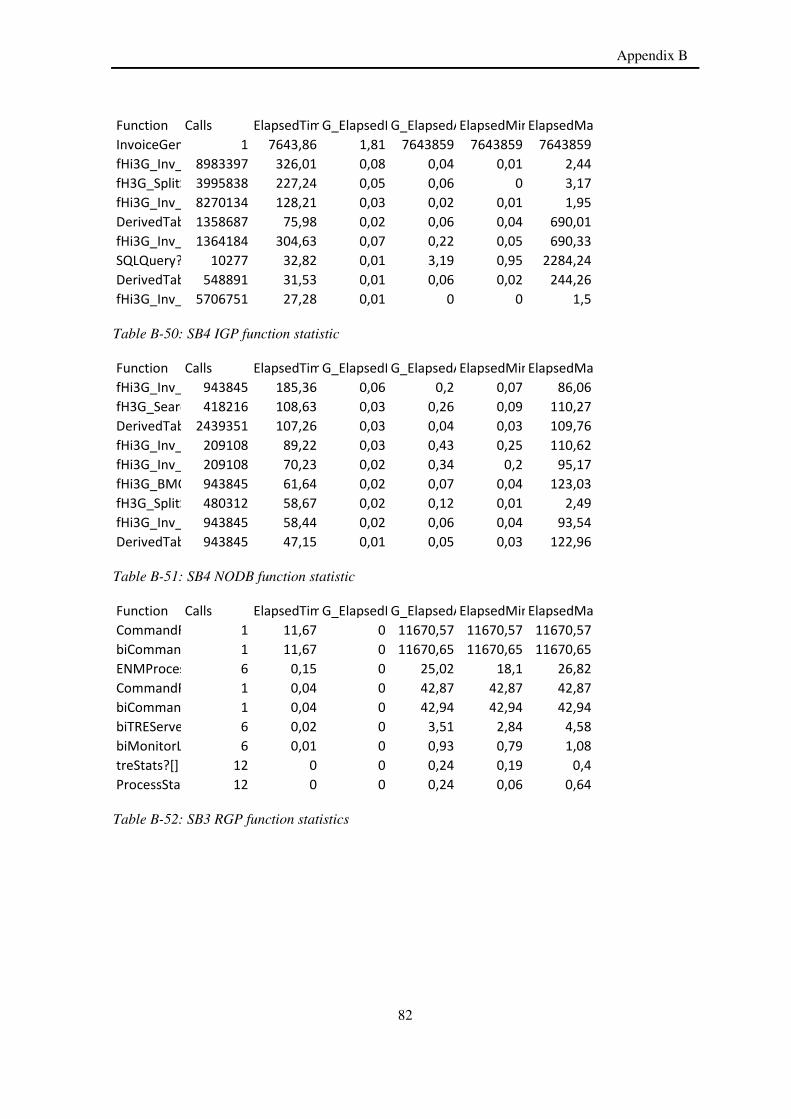
82
Appendix B
Function Calls ElapsedTimeG_ElapsedPerG_ElapsedAvgElapsedMinElapsedMax
InvoiceGenerate& 1 7643,86 1,81 7643859 7643859 7643859
fHi3G_Inv_GetSubString$8983397 326,01 0,08 0,04 0,01 2,44
fH3G_SplitString$[]3995838 227,24 0,05 0,06 0 3,17
fHi3G_Inv_GetSubStr$8270134 128,21 0,03 0,02 0,01 1,95
DerivedTableLookupByDatex&1358687 75,98 0,02 0,06 0,04 690,01
fHi3G_Inv_DeriveChargeFieldsInfo${}1364184 304,63 0,07 0,22 0,05 690,33
SQLQuery?[] 10277 32,82 0,01 3,19 0,95 2284,24
DerivedTableLookup&548891 31,53 0,01 0,06 0,02 244,26
fHi3G_Inv_IsDKCust&5706751 27,28 0,01 0 0 1,5
Table B-50: SB4 IGP function statistic
Function Calls ElapsedTimeG_ElapsedPerG_ElapsedAvgElapsedMinElapsedMax
fHi3G_Inv_AggregateUsageDetails&943845 185,36 0,06 0,2 0,07 86,06
fH3G_SearchMethod&418216 108,63 0,03 0,26 0,09 110,27
DerivedTableLookupByDatex&2439351 107,26 0,03 0,04 0,03 109,76
fHi3G_Inv_GetDestTxt$209108 89,22 0,03 0,43 0,25 110,62
fHi3G_Inv_GetCountryTxt$209108 70,23 0,02 0,34 0,2 95,17
fHi3G_BMC_GetSortCode$943845 61,64 0,02 0,07 0,04 123,03
fH3G_SplitString$[]480312 58,67 0,02 0,12 0,01 2,49
fHi3G_Inv_SEMergeUsageCategory$943845 58,44 0,02 0,06 0,04 93,54
DerivedTableLookupByDate&943845 47,15 0,01 0,05 0,03 122,96
Table B-51: SB4 NODB function statistic
Function Calls ElapsedTimeG_ElapsedPerG_ElapsedAvgElapsedMinElapsedMax
CommandRunGetResults&1 11,67 0 11670,57 11670,57 11670,57
biCommandRunGetResults&1 11,67 0 11670,65 11670,65 11670,65
ENMProcessNr& 6 0,15 0 25,02 18,1 26,82
CommandRun& 1 0,04 0 42,87 42,87 42,87
biCommandRun& 1 0,04 0 42,94 42,94 42,94
biTREServerMonitor&6 0,02 0 3,51 2,84 4,58
biMonitorLog& 6 0,01 0 0,93 0,79 1,08
treStats?[] 12 0 0 0,24 0,19 0,4
ProcessStats?{} 12 0 0 0,24 0,06 0,64
Table B-52: SB3 RGP function statistics

83
Appendix B
Function Calls ElapsedTimeG_ElapsedPerG_ElapsedAvgElapsedMinElapsedMax
RentalGenerate& 2 371,04 0,12 185520,6 183323 187718,3
biRentalGenerate& 2 371,04 0,12 185520,7 183323 187718,3
fH3G_NUC_RecurringChgElig&13761 34,39 0,01 2,5 1,69 387,89
biSQLQueryx& 13823 24,46 0,01 1,77 1,19 27,75
fH3G_DerivedTableContentsWpr?[]13823 5,64 0 0,41 0,27 97,94
fHi3G_RC_Eligibility&59 3,59 0 60,83 57,55 76,66
biSQLQueryRWx& 59 3,26 0 55,33 53,1 66,87
fH3G_SearchMethod&13823 2,84 0 0,21 0,14 266,47
DerivedTableLookupByDatex&27646 2 0 0,07 0,03 265,71
Table B-53: SB3 RODB function statistics
Function Calls ElapsedTimeG_ElapsedPerG_ElapsedAvgElapsedMinElapsedMax
biBillRunExecute& 1 35997,31 2,1 35997310 35997310 35997310
zBillRunProcessCustomers&8 35997,21 2,1 4499651 800,03 27964220
biInvoiceImageGenerate&1 27964,12 1,63 27964119 27964119 27964119
biBillRunInvoiceImageGenerate&1 27964,12 1,63 27964119 27964119 27964119
biInvoiceGenerate& 1 7643,88 0,45 7643876 7643876 7643876
biBillRunInvoiceGenerate&1 7643,88 0,45 7643876 7643876 7643876
biRentalGenerate& 2 371,06 0,02 185529,2 183338,9 187719,5
biSQLQueryx& 14286 191,72 0,01 13,42 0,66 24431,32
SQLQuery& 14289 190,69 0,01 13,34 0,65 24431,29
Table B-54: SB4 RWDB function statistics
Function Calls ElapsedTimeG_ElapsedPerG_ElapsedAvgElapsedMinElapsedMax
biSQLQueryRWx&3343 10,02 0 3 0,87 56,97
SQLQuery& 3344 9,96 0 2,98 0,86 56,95
zbiSearchAndFetch&72 2,41 0 33,42 3,98 167,9
biSQLQueryx& 72 2,25 0 31,26 2,24 164,82
ENMProcessNr& 31 1,52 0 49,08 17,61 151,53
biBillRunOperationSearchAndFetch&19 1,33 0 69,89 43,94 167,93
biTaskResultSearchAndFetch&45 0,92 0 20,52 4 135,79
SQLQuery?[] 2 0,35 0 174,93 20,82 329,03
zbiInvoiceAllocateForCustomer&1 0,33 0 329,08 329,08 329,08
Table B-55: SC6 BGP function statistics

84
Appendix B
Function Calls ElapsedTimeG_ElapsedPerG_ElapsedAvgElapsedMinElapsedMax
biInvoiceGenerate&51 30433,82 3,34 596741,5 5214,5 1723353
InvoiceGenerate& 51 30433,81 3,34 596741,5 5214,47 1723353
fHi3G_Inv_GetSubString$18412704 740,93 0,08 0,04 0,01 12,45
fH3G_AssignGLInfo&41097 643,6 0,07 15,66 0,17 150,64
fH3G_SplitString$[]10362187 641,92 0,07 0,06 0 7,55
SQLQuery& 56223 634,72 0,07 11,29 0,83 309,61
fHi3G_Inv_DeriveChargeFieldsInfo${}2261475 587,37 0,06 0,26 0,05 12,49
fH3G_GetGLCodeName&41077 573,35 0,06 13,96 0,04 131,46
fHi3G_AssignGLCode_Special&38389 511,85 0,06 13,33 0,19 150,71
Table B-56: SC6 IGP function statistics
Function Calls ElapsedTimeG_ElapsedPerG_ElapsedAvgElapsedMinElapsedMax
fH3G_SearchMethod&1992496 544,8 0,06 0,27 0,08 8,75
fHi3G_Inv_AggregateUsageDetails&1635365 506,97 0,06 0,31 0,07 6,84
SQLQuery& 36132 456,61 0,05 12,64 0,94 1923,28
fHi3G_Inv_GetDestTxt$996248 454,01 0,05 0,46 0,25 7,33
DerivedTableLookupByDatex&9057014 401,64 0,04 0,04 0,03 8,55
fHi3G_Inv_GetCountryTxt$996248 341,38 0,04 0,34 0,19 8,91
fHi3G_Inv_GetPackageCount&5001 329,66 0,04 65,92 13,38 1924,94
fH3G_SplitString$[]1531444 180,55 0,02 0,12 0,01 4,29
fHi3G_Inv_SEMergeUsageCategory$1635365 125,13 0,01 0,08 0,04 8,62
Table B-57: SC6 NODB function statistics
Function Calls ElapsedTimeG_ElapsedPerG_ElapsedAvgElapsedMinElapsedMax
CommandRunGetResults&51 542,97 0,03 10646,37 1123,9 11815,38
biCommandRunGetResults&51 542,97 0,03 10646,47 1123,99 11815,45
biCommandRun&5001 176,69 0,01 35,33 28,89 146,78
CommandRun& 5001 176,35 0,01 35,26 28,81 146,7
biTREServerMonitor&30 0,08 0 2,78 1,22 5,72
biMonitorLog& 30 0,03 0 0,98 0,4 2,44
treStats?[] 36 0,01 0 0,24 0,12 0,48
DerivedTableCacheStatistics&30 0 0 0,11 0,03 1,35
ProcessStats?{} 36 0 0 0,09 0,06 0,13
Table B-58: SC6 RGP function statistics

85
Appendix B
Function Calls ElapsedTimeG_ElapsedPerG_ElapsedAvgElapsedMinElapsedMax
biRentalGenerate&102 6365,65 0,7 62408,35 524,78 113101,4
RentalGenerate& 102 6365,64 0,7 62408,23 524,74 113101,3
fHi3G_RC_Eligibility&21260 1346,51 0,15 63,34 55,84 579,19
biSQLQueryRWx&21260 1210,59 0,13 56,94 51,71 571,92
biSQLQueryx& 86836 288,41 0,03 3,32 1,24 20650,35
fH3G_NUC_RecurringChgElig&53893 236,75 0,03 4,39 1,76 20652,18
fHi3G_NUC_CampaignRecurringChgElig&32943 147,59 0,02 4,48 1,84 98,01
fHi3G_Get_Base_Product_InstId?{}21260 133,43 0,01 6,28 3,36 129,14
biProductInstanceFetchById&21260 132,21 0,01 6,22 3,33 129,07
Table B-59: SC6 RODB function statistics
Function Calls ElapsedTimeG_ElapsedPerG_ElapsedAvgElapsedMinElapsedMax
biBillRunExecute& 51 82026,79 1,69 1608368 9348,24 6279599
zBillRunProcessCustomers&408 82026,5 1,69 201045,4 53,61 4328902
biBillRunInvoiceImageGenerate&51 39830,52 0,82 780990,6 536,75 4328871
biInvoiceImageGenerate&51 39830,51 0,82 780990,5 536,68 4328870
biBillRunInvoiceGenerate&51 33896,46 0,7 664636,4 5216,24 1723357
biInvoiceGenerate&51 33896,45 0,7 664636,2 5216,09 1723356
biRentalGenerate&102 6932,15 0,14 67962,24 526,22 134908,7
biBillRunRentalAdjustmentGenerate&51 3504,82 0,07 68721,87 526,29 134739,3
biBillRunRentalGenerate&51 3427,35 0,07 67202,9 904,23 134908,9
Table B-60: SC6 BGP function statistics
Function Calls ElapsedTimeG_ElapsedPerG_ElapsedAvgElapsedMinElapsedMax
SQLQuery& 64192 1267,36 0,01 19,74 0,6 569,08
biSQLQueryRWx&58527 1257,35 0,01 21,48 0,73 569,1
zbiInvoiceAllocateForCustomer&5001 110,64 0 22,12 1,48 1944,54
SQLQuery?[] 10002 106,12 0 10,61 0,74 312,61
SQLExecute& 50010 85,15 0 1,7 0,69 151,5
biSQLExecutex&25005 60,94 0 2,44 0,69 151,52
biCustomerNodeBillRunUpdate&10002 38,56 0 3,86 1,95 59,95
biInvoiceReportAccounts&5001 32,98 0 6,59 3,63 95,76
biCustomerNodeUnlock&10002 16,86 0 1,69 0,83 50,27

86
Appendix C
Appendix C
Files
File C-1: Default BGP configuration file.
1. [BGP.1] 2. Name=BGP1 3. Group=6 4. CUSTOMER_CHILD_PROCESSES=0 5. NODE_CHILD_PROCESSES=0 6. SERVICE_CHILD_PROCESSES=0 7. EVENT_CHILD_PROCESSES=0 8. SERVICE_MIN_EVENTS=0 9. EVENT_PERIOD=0 10. EVENT_PERIOD_TYPE=Days 11. NON_GLOBAL_DA_CACHE_SIZE=100 12. GLOBAL_DA_CACHE_SIZE=100 13. DISABLE_HASH_JOIN=False 14. DEBUG_LEVEL= 15. ERROR_THRESHOLD=100 16. USAGE_CHARGES_BEFORE_BILL_DATE=False 17. STATISTICS_TIMEOUT= 18. STATISTICS_FUNCTION=BGPLogStatistics& 19. VARIABLE_CACHE_SIZE=700
File C-2: BGP configuration file two.
1. [BGP.2] 2. Name=BGP2 3. Group=6 4. CUSTOMER_CHILD_PROCESSES=0 5. NODE_CHILD_PROCESSES=2 6. SERVICE_CHILD_PROCESSES=4 7. EVENT_CHILD_PROCESSES=0 8. SERVICE_MIN_EVENTS=0 9. EVENT_PERIOD=0 10. EVENT_PERIOD_TYPE=Days 11. NON_GLOBAL_DA_CACHE_SIZE=100 12. GLOBAL_DA_CACHE_SIZE=100 13. DISABLE_HASH_JOIN=False 14. DEBUG_LEVEL= 15. ERROR_THRESHOLD=100 16. USAGE_CHARGES_BEFORE_BILL_DATE=False 17. STATISTICS_TIMEOUT= 18. STATISTICS_FUNCTION=BGPLogStatistics& 19. VARIABLE_CACHE_SIZE=700
File C-3: Part of the original ubbconfig file
# trebgp for ordinary billing configuration trebgp SRVGRP=BILLING SRVID=200 RESTART=Y MAXGEN=5 CLOPT="-A -- BGP1" MIN=3 MAX=12 SEQUENCE=6
Code
In this section shows a few of the code pieces that were written for this project other codes were stored in the UAT2 environment.
Code C-1: SQL code to create profile table
def profile_start_date = '''01-SEP-2007''' def profile_end_date = '''01-OCT-2007''' create table SERVICE_PROFILE as

87
Appendix C
(select service_id, count(*) charge_count from charge where charge_date between to_date(&profile_start_date, 'dd-mon-yyyy') and to_date(&profile_end_date, 'dd-mon-yyyy') and customer_node_id is null group by service_id); create table CUSTOMER_NODE_PROFILE as (select s.customer_node_id, count(s.service_id) service_count, count(sp.service_id) active_service_count, sum(sp.charge_count) charge_count from service_history s, service_profile sp where sysdate between s.effective_start_date and s.effective_end_date and s.service_id = sp.service_id (+) group by s.customer_node_id); create table CUSTOMER_PROFILE as (select nvl(cnh.root_customer_node_id, cnh.customer_node_id) customer_node_id, count(*) node_count, sum(cnp.service_count) service_count, sum(cnp.active_service_count) active_service_count, sum(cnp.charge_count) charge_count from customer_node_history cnh, customer_node_profile cnp where sysdate between cnh.effective_start_date and cnh.effective_end_date and cnh.customer_node_id = cnp.customer_node_id (+) group by nvl(cnh.root_customer_node_id, cnh.customer_node_id)); create table SCHEDULE_PROFILE as (select cnh.schedule_id, count(*) customer_count, sum(pcf.node_count) node_count, sum(pcf.service_count) service_count, sum(pcf.active_service_count) active_service_count, sum(pcf.charge_count) charge_count from customer_node_history cnh, customer_profile pcf where sysdate between cnh.effective_start_date and cnh.effective_end_date and cnh.customer_node_id = pcf.customer_node_id group by cnh.schedule_id);
Code C-2: SQL code to update BGP service
update customer_node_history cnh set billing_configuration_code = 2 where customer_node_id in ( select tdata.customer_node_id from testuser.hmw_testsb3 tdata, testuser.customer_profile tcp where tcp.customer_node_id = tdata.customer_node_id and tcp.active_service_count >=4 );
Code C-3: Singl.eView code fHi3G_GetGLCodeHash?{}
fHi3G_GetGLCodeHash?{}() = { constconstconstconst cSQLText$ :='SELECT GL_CODE_ID,GL_CODE_NAME,ACCOUNT_CLASS_CODE,'+ ' EFFECTIVE_START_DATE, EFFECTIVE_END_DATE '+ ' FROM GL_CODE_HISTORY '; varvarvarvar resultHash?{}; varvarvarvar rows?[]; varvarvarvar i&; #Fetch all gl-codes rows?[] := SQLQuery?[](cSQLText$, [], []); #Build an hash with the information retrieved with the query forforforfor(i&:=0;i&<sizeof(rows?[]);i&++) { #Check if more than 1 history record ifififif ( !exists(resultHash?{}, to_string(rows?[i&][0])) ) { resultHash?{to_string(rows?[i&][0])}[] := [[to_string(rows?[i&][1]), to_string(rows?[i&][2]), rows~[i&][3], rows~[i&][4]]];

88
Appendix C
} elseelseelseelse { push(resultHash?{to_string(rows?[i&][0])}[],[to_string(rows?[i&][1]), to_string(rows?[i&][2]), rows~[i&][3], rows~[i&][4]]); } } returnreturnreturnreturn transfer(resultHash?{}); }
Code C-4: Singl.eView code fH3G_GetGLCodeName&
fH3G_GetGLCodeName&(constconstconstconst cGLCodeId&, constconstconstconst cGLDate~, varvarvarvar outGLString$, varvarvarvar outGLAccountCC$) = { cocococonstnstnstnst glHash?{} := fHi3G_GetGLCodeHash?{}(); constconstconstconst cGLStringIdx& := 0; constconstconstconst cGLAccountIdx& := 1; constconstconstconst cGLEffStartDateIdx& := 2; constconstconstconst cGLEffEndDateIdx& := 3; varvarvarvar i&; ifififif ( length(glHash?{to_string(cGLCodeId&)}[]) = 1 ) { # Return values immedatley outGLString$ := glHash${to_string(cGLCodeId&)}[0][cGLStringIdx&]; outGLAccountCC$ := glHash${to_string(cGLCodeId&)}[0][cGLAccountIdx&]; returnreturnreturnreturn 1; }elseelseelseelse { forforforfor(i&:=0; i& < sizeof(glHash?{to_string(cGLCodeId&)}[]); i&++) ifififif ( cGLDate~ >= glHash~{to_string(cGLCodeId&)}[i&][cGLEffStartDateIdx&] && cGLDate~ <= glHash~{to_string(cGLCodeId&)}[i&][cGLEffEndDateIdx&] ) { # iter over array until glHash?{to_string(glCodeId&)}[] GLDate between #startdate end date outGLString$ := glHash${to_string(cGLCodeId&)}[i&][cGLStringIdx&]; outGLAccountCC$ := glHash${to_string(cGLCodeId&)}[i&][cGLAccountIdx&]; returnreturnreturnreturn 1; } } returnreturnreturnreturn 0 }

89
Appendix D
Appendix D
RAID description
RAID stands for Redundant Array of Independent Disks or Redundant Arrays of Inexpensive Disks. There are several levels of settings that have different impact on the hard drives storage behavior.
RAID 1 is also called disk mirroring and it requires two disks with the same storage size. The secondary disk creates an identical copy of the main disk and will improve the read performance because two hard drives can fetch the data simultaneously. This setting provides safety for the data when one disk is malfunctioning. Writing data may affect the performance.
RAID 5 requires at least one hard drive of disk space for checksum storage and writes the error code as an array across the entire disk setup. The checksum is used for detecting errors across the disks and recreating the lost data on the other disks. This setting is using the striping method by splitting the files into parts that are stored on numerous disks. This will increase the performance on both read and write operations. When one disk is malfunctioning it will cause decreasing read performance [7].

TRITA-CSC-E 2008:046 ISRN-KTH/CSC/E--08/046--SE
ISSN-1653-5715
www.kth.se