THE PATHFINDER PROGRAM AND ITS APPLICATION TO ION OPTICS

by

P.J. STENNING1 and C.W. TROWBRIDGE2 ABSTRACT The FORTRAN computer program "Pathfinder" is described. This program calculates the electrostatic potential distribution for a defined translationally or rotationally symmetric electrode configuration and determines the trajectories of charged particles through the resultant electric field. A correlation with an analytic solution is made in order to demonstrate the validity of the program; these results indicate that accuracies of less than 0.5% can be achieved. The program is further checked by comparison with the best available experimental data on electrostatic lenses. 'Pathfinder' is then applied to several systems used in ion optics with special reference to aberrations, in particular: (1) Various configurations of einzel lenses (2) The cross-over or matching gap lens (3.) The accelerator tube, for which results of special interest are derived (4) Individual lens systems. May 1968 Note This version of the above paper has been transcribed into MS WORD by C W Trowbridge (Nov. 2002) now at Vector Fields Ltd, Oxford; contact E-Mail address bill@trowbridge.org.uk. The paper has some historical value as an early example of scientific computer based tool long since superseded but the results still have relevance today, particularly in the design of accelerator tubes as several citations in the literature show.

1 Department of Physical Sciences The University of Reading Berkshire 2 Rutherford Laboratory Science Research Council Chilton, Didcot, Oxon

1

Contents

1. INTRODUCTION 3

2. THE PROGRAM AND ITS EFFECTIVENESS 3 2.1 The Action of Pathfinder 3 2.2 Validity of Pathfinder 5 2.3 The Measurement of Spherical Aberration using the Computer Program 6 2.4 Some Computer Comparisons 7

(a) Three Configurations analysed by Ramberg [4] 7 (b) Three configurations investigated by Liebmann [6] 8 (c) Some Septier Configurations 8

3 THE ION-OPTICAL PROPERTIES OF SOME ELECTROSTATIC SYSTEMS 9 3.1 Einzel Lenses 9

(a) The shape of the electrodes 9 (b) The Cylindrical Einzel Lens 9

3.2 The Gap Lens 10 (a) The Practical Performance of the Gap Lens 10 (b) The Shape of the Electrodes 11 (c) Comparison with a Graduated Potential Lens 11

3. 3 Accelerator Tubes 11 3. 4 The Aperture Lens 12

4 APPLICATION TO A COMPLETE SYSTEM 14 4. The Ion Source Lens 14 4.2 The Gap Lens 14 4.3 The Accelerator Tube 14

5. CONCLUSION 15

ACKNOWLEDGEMENTS 15

REFERENCES 16

APPENDIX I 17

APPENDIX II 18

FIGURES 20

2

1. Introduction In the past, a wealth of information has been published on the properties of electrostatic lenses [1]. Experimental: determinations of the potential distributions within lenses have been made using electrolytic tank and resistance network techniques; theoretical determinations have assumed simplified boundary conditions or have been by relaxation methods. The optical properties have been found by various parallel beam and grid shadow experiments, or by integration of the paraxial ray equation and graphical ray tracing methods. There are many techniques which are helpful in the design of lenses to meet specific requirements. However there is still no general method by which to exactly predict the aberrations of a given system without recourse to at least numerical integration of the axial potential distribution, itself frequently only an approximation. We decided to use the computer from the beginning, to simulate practical cases and obtain readily usable results. The program Pathfinder produces both numerical values of the potential distribution for an extremely wide range of electrode-configurations, and the trajectories of charged particles through these electrode systems. It may be used for ray tracing in plane two dimensional systems and for those with axial symmetry; the latter case is applicable to rotationally symmetric lenses. The program is at present neither relativistic nor does it take account of space charge, or treat skew rays. In what follows, Section 2 discusses the "Pathfinder' program and its modus operandi, and presents the analytic check and comparison with some experimental results. The choice of these comparisons themselves is no easy matter, since the reliability of most of the experimental results is open to some question, as even with accurate measuring, techniques, variation of the conditions within the vacuum chamber enclosing the apparatus can cause not-insignificant changes in the optical properties of the lens under investigation, e.g. a mono-layer of hydro-carbon from the vacuum pumps deposited on the electrodes can cause charge to build up on them, with corresponding perturbations of the fields. The analytic configuration checks make it apparent that the program is capable of considerable accuracy, and the experimental comparisons, with one or two notable exceptions, show good agreement. Section 3 deals with various electrostatic systems, viz:- The einzel lens (b) The gap lens (c) Accelerator tubes (d) The aperture lens. Some of the ion-optical properties of these are given, with special reference to spherical aberration. From the results obtained, it seems that from the point of view of aberrations, the simple einzel 1ens is as effective as any of the much more complicated systems. By way of an illustration, Section 4 deals with the optics of a complete system:- the Injector System for the Oxford Electrostatic Generator.

2. The Program and Its Effectiveness

2.1 The Action of Pathfinder

The program is written in. FORTRAN and current versions are available for use with the I.C.T. Atlas Computer and the IBM 360/75 at the Rutherford Laboratory. The program is in two main parts. The first generates a suitable mesh based on the specified boundaries and

3

solves Laplace's equation to obtain the potential distribution. This part is based on a program developed at CERN, and its detailed mode of operation is described elsewhere [3]. The second part determines the paths of particles through the electrostatic field by solving the dynamical equations of motion; for systems with axial symmetry these are:

2.1 2 2

2 2

// /

md r dt e V rmd z dt e V z

= ∂ ∂

= ∂ ∂

/

The method used to determine the particle trajectories is essentially that due to Goddard [4]. At each stage of the trajectory calculation, the values of the components of accelerations in equation (2.1) are determined by numerical differentiation of the potential in the neighbourhood of the particle coordinates. The next stage is then calculated by suitable Lagrangian formulae using the gradients at the present stage and the co-ordinates and gradients at several of the proceeding stages. The exact formulae used depend on the number of previous stages available, viz: Four or less

2

1

1

12m m m

m m m

z z Tz T

z z Tz

+

+

= + +

= +

mz 2.2

Five, Six or Seven

2

1 2 3 1

1 1 2

1 (5 2 5 )4

(23 16 5 ) /12

m m m m m m m

m m m m m

z z z z T z z z

z z T z z z

+ − − −

+ − −

= + − + + +

= + − +

2− 2.3

More than Seven

21 4 5 1 2 3 4

1 1 2

(67 8 122 8 67 ) / 48(23 16 5 ) /12

m m m m m m m m m

m m m m m

z z z z T z z z z zz z T z z z

+ − − − − − −

+ − −

= + − + + + − += + − +

2.4

4

where z is the position coordinate after m+1 steps, and are the associated velocity and acceleration and T is the time interval. There is a similar set of equations for the radial co-ordinates.

z z

The values for the starting equation (2.2) are determined from the initial conditions; the time interval between steps is set by the time taken to transit one potential mesh at the initial velocity. At each stage of the calculation the energy of the particle is computed from the velocity components and compared with the interpolated value of the potential. This enables a check to be made on the accuracy and the time interval is automatically decreased until an error criterion is satisfied. In the present version the time interval is halved until the error is less than a specified amount. In the print out of results the spatial coordinates, velocity components and accelerations are tabulated. Also a graphical output may be obtained on which are depicted the potential boundaries and the particle paths. When using the program for ion optical systems the print out gives the optical constants. There is a third part of the program which calculates the paraxial focal lengths of systems by direct integration of the axial potential.

2.2 Validity of Pathfinder In order to assess the validity of the program it was necessary to find some configuration for which an analytic solution exists, so that a comparison between results obtained by numerical techniques and theory could be made. Initially, the program was checked against Goddard’s [12] values for the focal lengths of two cylinder lenses, in which he uses Bertram's formula for the axial potential distribution. No detailed comparison of actual potentials was made however, as it was decided to use a configuration with a mathematically simpler solution, and one for which relatively simple trajectory equations could be found. Neglecting as trivial the case of a uniform field in plane symmetry (e.g. two infinite parallel plates with a uniform gradient between), it can be shown that with axial symmetry Laplace's equation is completely solved by a certain family of hyperbolic equipotentials defined by:-

2 21 1( )2 2

z rφ λ C= − + 2.5

i.e. the set of hyperbolae whose common asymptote intersects the z axis at an angle given by

1tan ( 2)− . In 2.5,

2.6 2 2

2 1 2 12 2 2

2 1 1 2 1

2( ) /( )

( ) /(

V V q q

C V V q q q

λ = − −

= − − − )

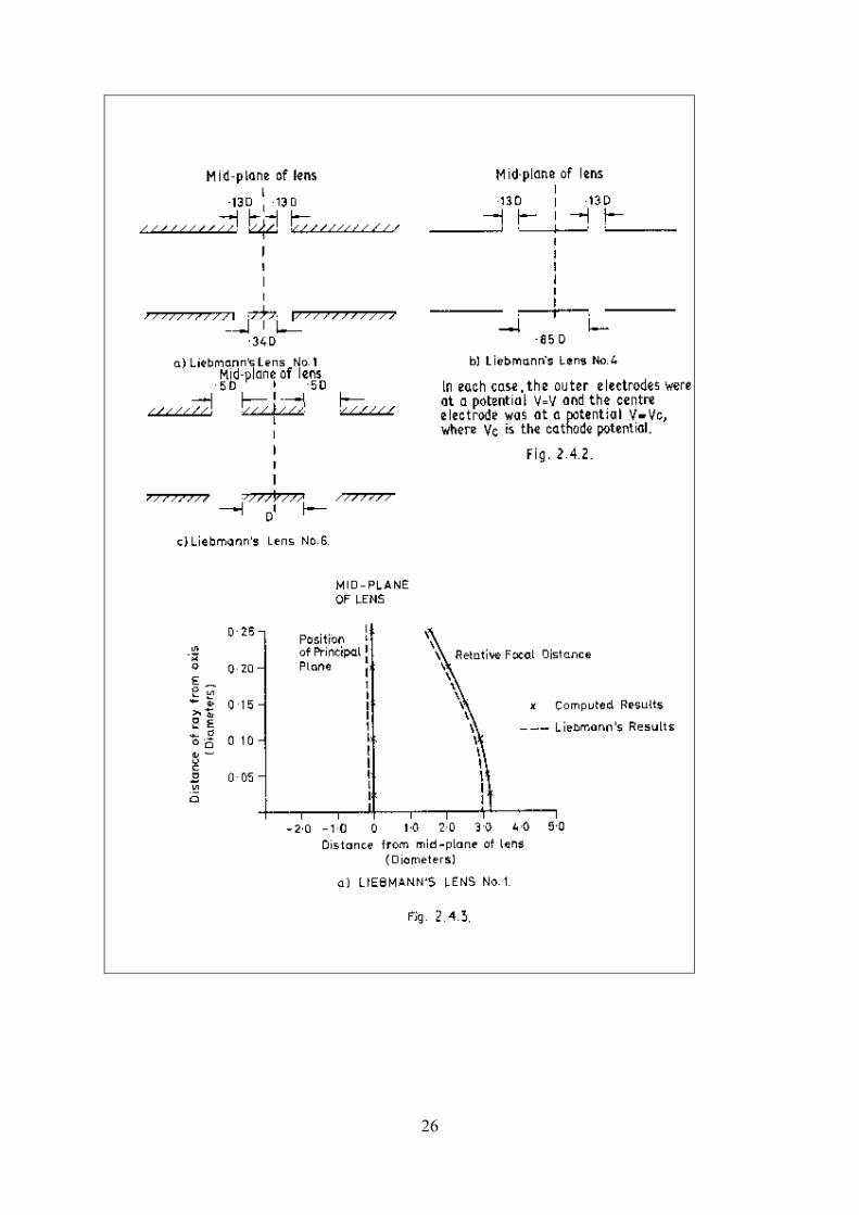
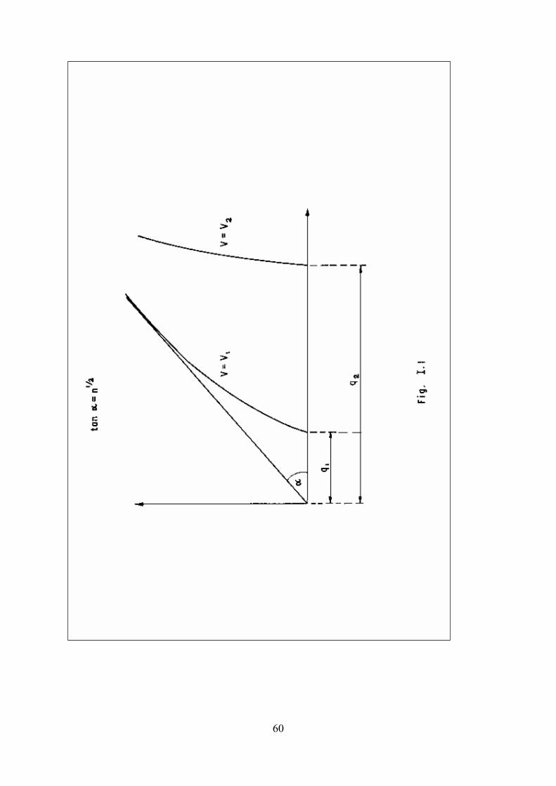
where V1 and V2 are the potentials at distances q1 and q2 from the origin along the z axis. Fig 2.2.1 shows the equipotentials appropriate to V=V1 and V=V2 where V is the potential at any point in space. A complete derivation of equations 2.5 and 2.6 is given in Appendix L. It may also be shown (see Appendix II) that in the above system for any plane through the axis of symmetry the position co-ordinates of charged particles are defined by:-

5

1

1 2

2 2 2 10 0

1 0 0 2 0

cos ( / 2 ) exp( ) exp( )

where ( 2 / ) , tan ( 2 / )and ( ) / 2 , C (

r k Ez C kt C kt

A r r k E r krC kz z k kz

−

−

= += + −

= + =

= + = − 0 ) / 2 , /z k k eλ=0

m

0z

2.8

r0 and z0 define the initial position, are the initial component velocities. Arbitrarily, the following conditions were chosen:-

0 and r

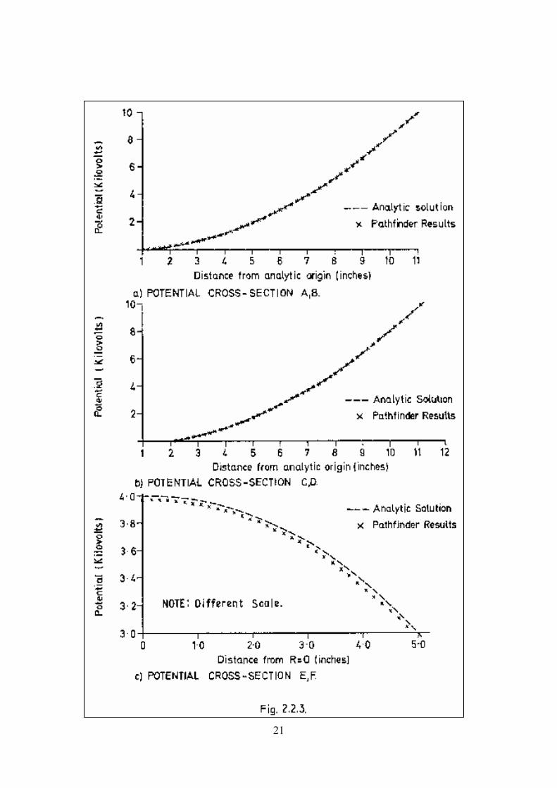
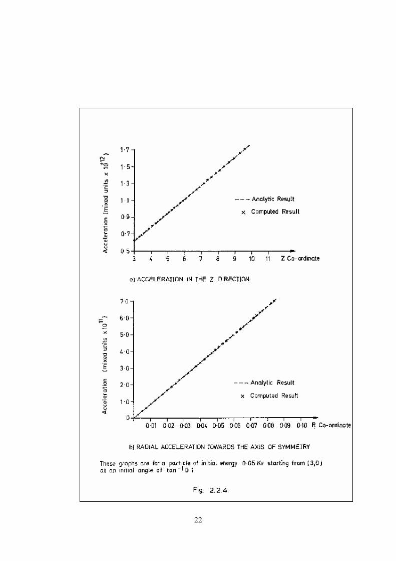
V1 =0, V2 =10, q1=1, and q2 =11. Pathfinder was given as its input configuration the area shown in Fig. 2.2.2 and a series of particle trajectories were computed. These were then checked against the exact solutions given by equations 2.8. Fig. 2.2.3 shows comparisons between the potential distribution obtained from the program and that predicted theoretically. The comparisons shown in the figures are for the potential distributions along lines ab, cd and ef in Fig. 2.2.2. It should be noted that the potential distribution along ef in Fig. 2.2.3 is plotted to a different scale than those along ab and ed; this diagram indicates that the potentials are accurate to better than 0.5%. Only the field (i. e. the rate of change of potential, the slope of the graph) is required to calculate the trajectories however, and this follows the analytic solution even more closely. All other potential and, field values considered compared at least as favourably as these. As can be seen in Appendix II, the components of the acceleration are given by:-

12

r

z kz

= −

=

kr 2.9

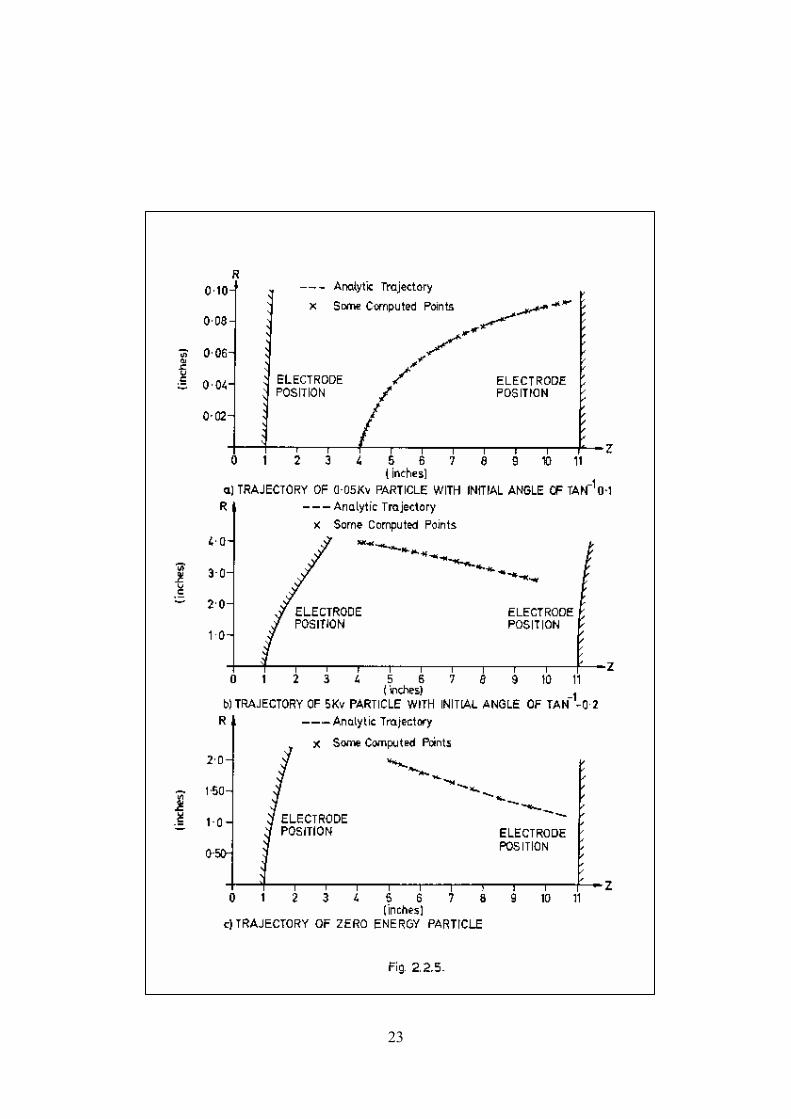
The computed and analytic results for accelerations are shown in Fig. 2.2.4. The ultimate test of the program is the comparison of actual trajectories. Fig, 2.2.5 shows three such comparisons covering a wide range of particle initial conditions. In each of these almost exact agreement between the computed and analytic results is demonstrated. Several other trajectory comparisons were made with equally favourable results. From these results it is estimated that the program produces trajectories which are accurate to at least one half per cent.

2.3 The Measurement of Spherical Aberration using the Computer Program

The Gaussian Theory of electron optics predicts a point focus for all rays emanating from an object and so a perfect image. This approaches the truth only under paraxial conditions however. With non-paraxial rays a wide variety of discrepancies from the ideal occur, and these are termed the aberrations. The mathematical theory of aberrations is already covered by an extensive literature and will pot be described here. Suffice it to say that to the next order of accuracy each of these radial deviations from the Gaussian Theory may be represented by a third order term. We are particularly concerned with the greatest of these,

6

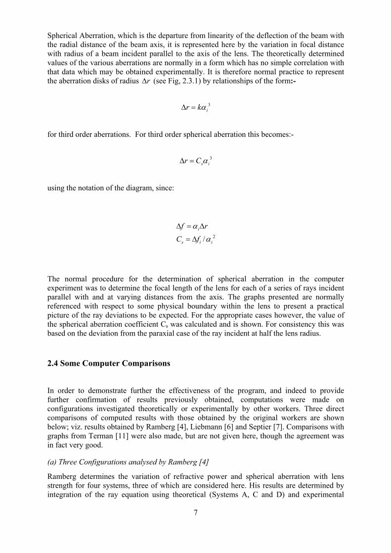
Spherical Aberration, which is the departure from linearity of the deflection of the beam with the radial distance of the beam axis, it is represented here by the variation in focal distance with radius of a beam incident parallel to the axis of the lens. The theoretically determined values of the various aberrations are normally in a form which has no simple correlation with that data which may be obtained experimentally. It is therefore normal practice to represent the aberration disks of radius (see Fig, 2.3.1) by relationships of the form:- r∆

3ir kα∆ =

for third order aberrations. For third order spherical aberration this becomes:-

3s ir C α∆ =

using the notation of the diagram, since:

2/

i

s i i

f r

C f

α

α

∆ = ∆

= ∆

The normal procedure for the determination of spherical aberration in the computer experiment was to determine the focal length of the lens for each of a series of rays incident parallel with and at varying distances from the axis. The graphs presented are normally referenced with respect to some physical boundary within the lens to present a practical picture of the ray deviations to be expected. For the appropriate cases however, the value of the spherical aberration coefficient Cs was calculated and is shown. For consistency this was based on the deviation from the paraxial case of the ray incident at half the lens radius.

2.4 Some Computer Comparisons

In order to demonstrate further the effectiveness of the program, and indeed to provide further confirmation of results previously obtained, computations were made on configurations investigated theoretically or experimentally by other workers. Three direct comparisons of computed results with those obtained by the original workers are shown below; viz. results obtained by Ramberg [4], Liebmann [6] and Septier [7]. Comparisons with graphs from Terman [11] were also made, but are not given here, though the agreement was in fact very good.

(a) Three Configurations analysed by Ramberg [4]

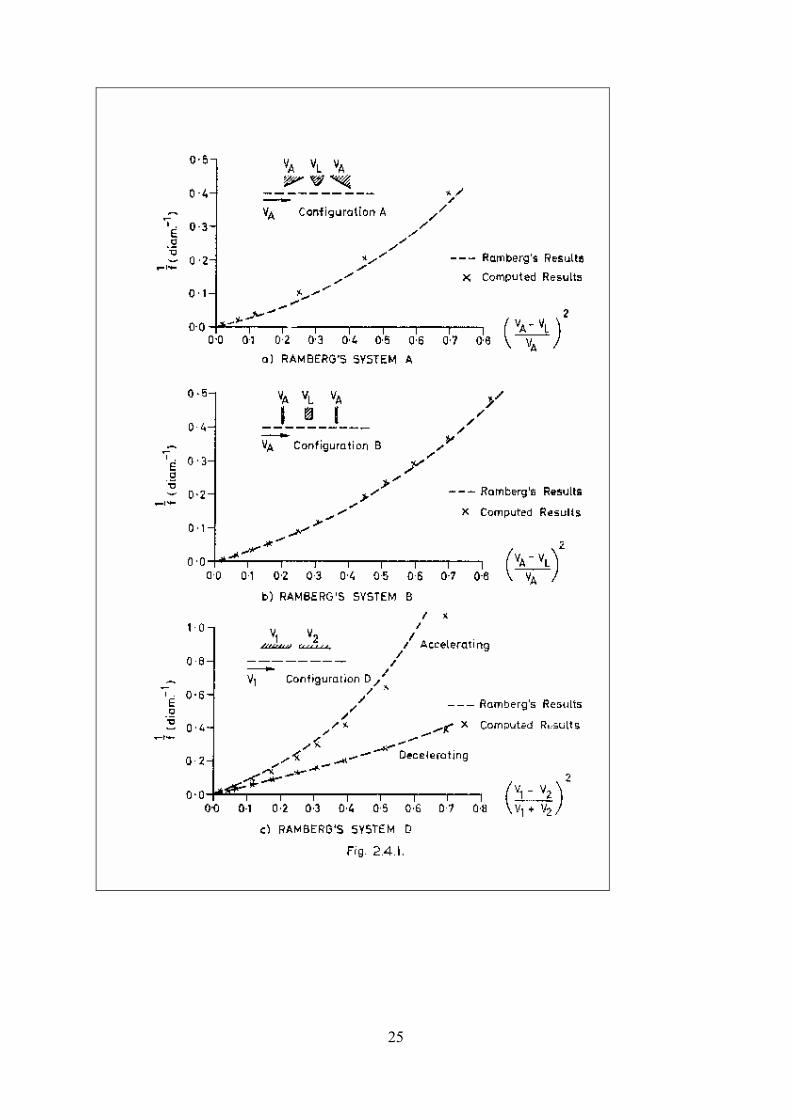
Ramberg determines the variation of refractive power and spherical aberration with lens strength for four systems, three of which are considered here. His results are determined by integration of the ray equation using theoretical (Systems A, C and D) and experimental

7

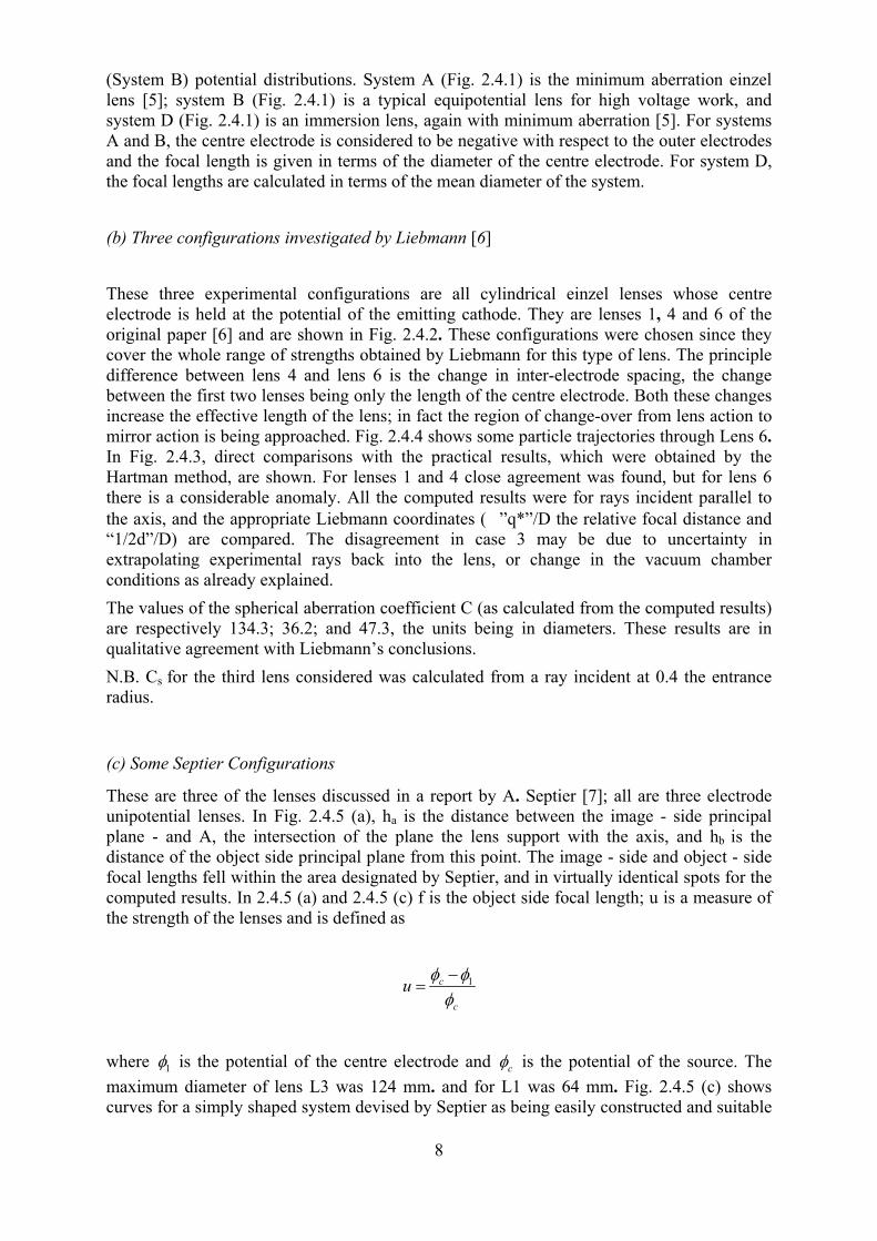
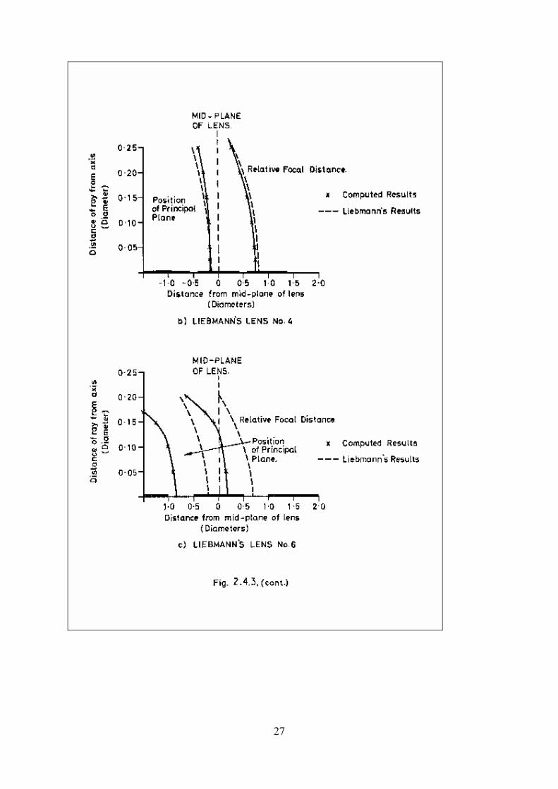
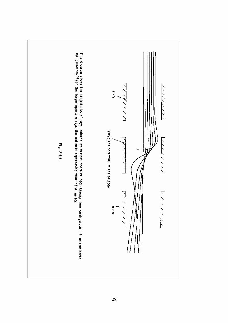
(System B) potential distributions. System A (Fig. 2.4.1) is the minimum aberration einzel lens [5]; system B (Fig. 2.4.1) is a typical equipotential lens for high voltage work, and system D (Fig. 2.4.1) is an immersion lens, again with minimum aberration [5]. For systems A and B, the centre electrode is considered to be negative with respect to the outer electrodes and the focal length is given in terms of the diameter of the centre electrode. For system D, the focal lengths are calculated in terms of the mean diameter of the system. (b) Three configurations investigated by Liebmann [6] These three experimental configurations are all cylindrical einzel lenses whose centre electrode is held at the potential of the emitting cathode. They are lenses 1, 4 and 6 of the original paper [6] and are shown in Fig. 2.4.2. These configurations were chosen since they cover the whole range of strengths obtained by Liebmann for this type of lens. The principle difference between lens 4 and lens 6 is the change in inter-electrode spacing, the change between the first two lenses being only the length of the centre electrode. Both these changes increase the effective length of the lens; in fact the region of change-over from lens action to mirror action is being approached. Fig. 2.4.4 shows some particle trajectories through Lens 6. In Fig. 2.4.3, direct comparisons with the practical results, which were obtained by the Hartman method, are shown. For lenses 1 and 4 close agreement was found, but for lens 6 there is a considerable anomaly. All the computed results were for rays incident parallel to the axis, and the appropriate Liebmann coordinates ( ”q*”/D the relative focal distance and “1/2d”/D) are compared. The disagreement in case 3 may be due to uncertainty in extrapolating experimental rays back into the lens, or change in the vacuum chamber conditions as already explained. The values of the spherical aberration coefficient C (as calculated from the computed results) are respectively 134.3; 36.2; and 47.3, the units being in diameters. These results are in qualitative agreement with Liebmann’s conclusions. N.B. Cs for the third lens considered was calculated from a ray incident at 0.4 the entrance radius.

(c) Some Septier Configurations

These are three of the lenses discussed in a report by A. Septier [7]; all are three electrode unipotential lenses. In Fig. 2.4.5 (a), ha is the distance between the image - side principal plane - and A, the intersection of the plane the lens support with the axis, and hb is the distance of the object side principal plane from this point. The image - side and object - side focal lengths fell within the area designated by Septier, and in virtually identical spots for the computed results. In 2.4.5 (a) and 2.4.5 (c) f is the object side focal length; u is a measure of the strength of the lenses and is defined as

1c

c

u φ φφ−

=

where 1φ is the potential of the centre electrode and cφ is the potential of the source. The maximum diameter of lens L3 was 124 mm. and for L1 was 64 mm. Fig. 2.4.5 (c) shows curves for a simply shaped system devised by Septier as being easily constructed and suitable

8

for normal practical use. This was one of the configurations which led to an optimum lens, which is shown in Section , 3.1 (a). The maximum diameter of the lens was 150 mm. All computations were for parallel incident rays. Septier's results were obtained by photographing, at various positions after the lens, the shadow on a screen of a beam which was incident parallel to the axis of symmetry, and from these photographs at known positions calculating the actual trajectories. He claimed an accuracy of; 5% in positioning. The computed results for his lens L3 agree to within this accuracy, as do the results over certain strength values for lens L1. For lens L5 and for lens L1 at lower strength however, agreement is at best only within 10%. Again, there several possible explanations for the discrepancies.

3 The Ion-optical Properties of some Electrostatic Systems

3.1 Einzel Lenses

(a) The shape of the electrodes

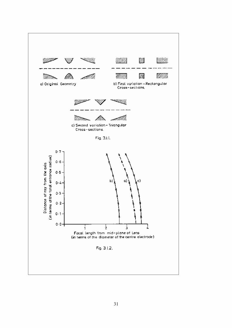
The geometry for the three electrode lens with minimum spherical aberration has been derived theoretically by Plass [5] and analysed by Ramberg [4]. The computed results for the variation of the focal length with lens strength have already been presented in Section 2.4 (a). In order to try and determine the practical importance of shaping the electrodes as specified, the spherical aberration curves for this lens and two simpler variations thereof (Fig. 3.1.1) were computed, and are shown in Fig. 3.1.2. In all cases, the cross-sectional area of the electrodes was constant. As can be seen, large quantitative changes in focal length occur, but little change in the percentage variation of focal length with beam radius. For a true comparison of the aberration coefficient of the three lenses, the aberration coefficient Cs must again be considered. Using this criterion, the geometric change into rectangular cross-section seems to provide an improvement, as indeed it does, but to evaluate the comparative merits of the lenses, the magnification should also be considered. (See Reference [7]). From the general trend of the results, which are as would be expected, it would seem that for ,'the "changes in focal length, it would seem that for a given focal length there is little need for specific complex shaping. Fig. 3.1.3 shows the spherical aberration curve for Septier's experimentally optimised asymmetric three electrode lens [7]. A simpler geometry is again compared, with a similar result. All computations were performed for rays incident parallel to the axis.

(b) The Cylindrical Einzel Lens

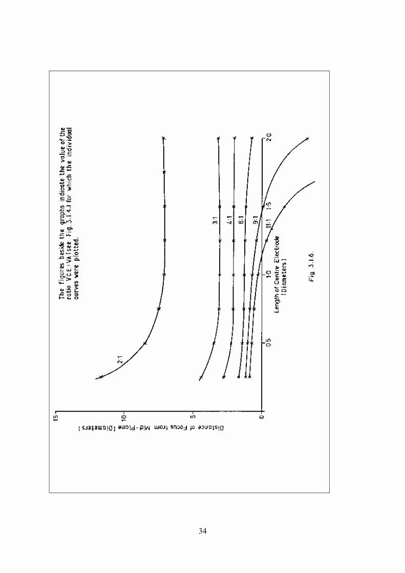
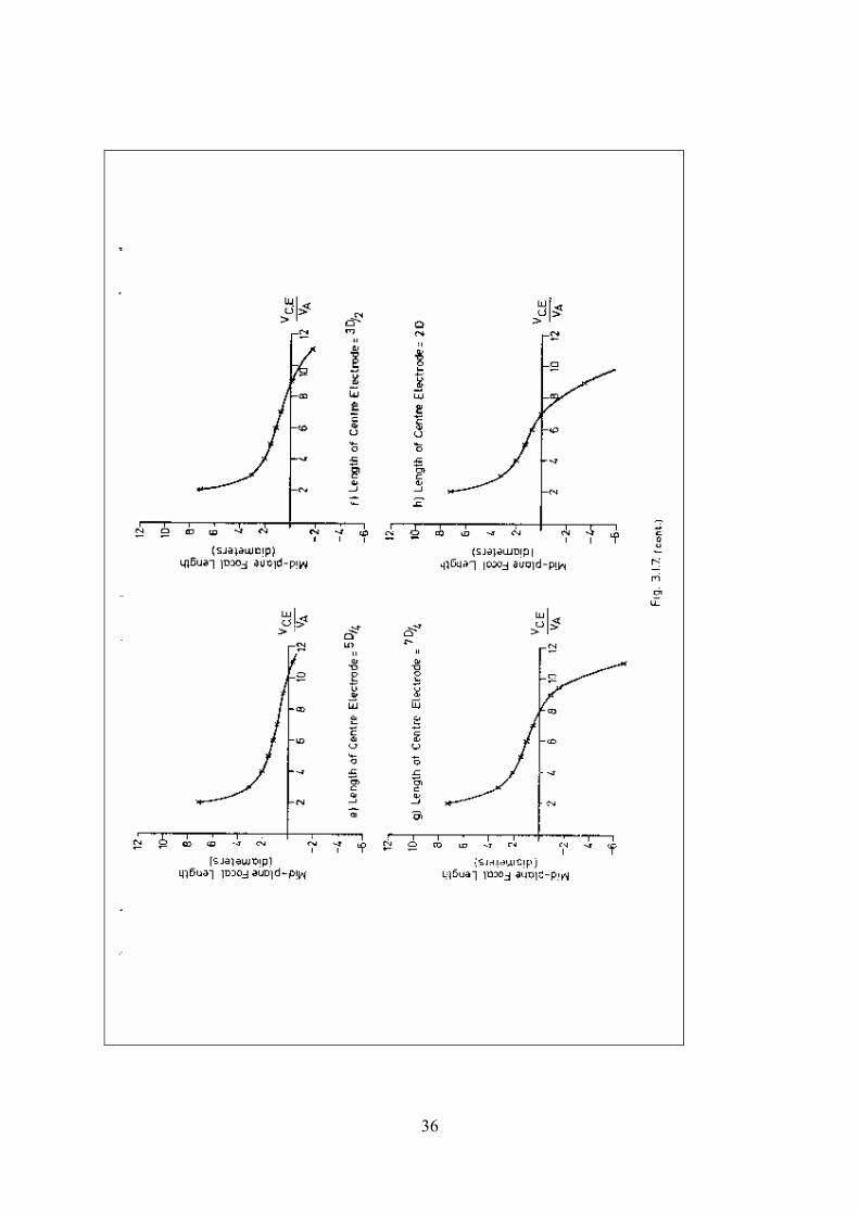
A systematic study of the cylindrical einzel lens with constant diameter was made to determine the effect of the variation in length of the centre electrode. The inter-electrode spacing was held constant at D/4, and computations made for various strengths. In the first place the centre electrode was made positive with respect to the outer electrodes, producing an accelerating, decelerating action. Rays incident parallel to the axis were considered. The basic configuration is shown in Fig. 3.1.4. Fig. 3.1.5 shows a typical aberration curve for the lens in this mode. These were similar for all strengths, so the results presented hereafter are for the axial focal lengths, i.e. the position in which a ray incident parallel to, and at an infinitesimal distance from the axis, would focus. Fig. 3.1.6 shows the variation in focus with the length of the centre electrode, for various values of the ratio Vce : Va, the voltages defined in Fig. 3.1.4. It can be seen that for the

9

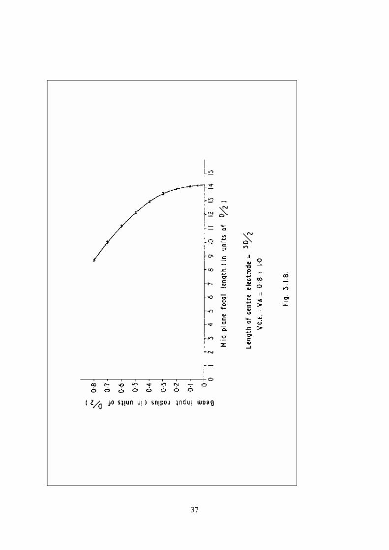
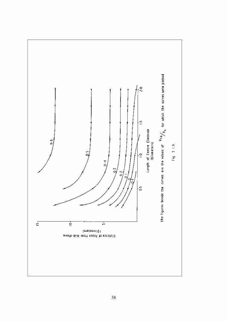
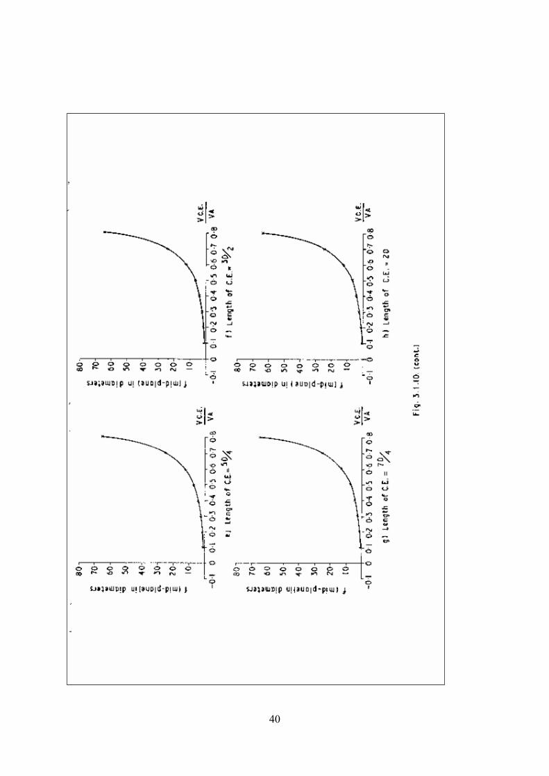
medium strength lenses (Vce : Va = 3:1 to 6:1), elongation of the centre electrode beyond D/2 produces little variation in focus. Fig. 3.1.7 shows plots of focal length against Vce/Va for various centre electrode lengths, and includes results for lens strengths not shown in Fig. 3.1.6. Secondly, the centre electrode was made negative w.r.t. the outer electrodes, producing a decelerating - accelerating action. The geometries of the configurations considered were identical to those of the first case, as were the position parameters of the input rays, and the corresponding results are shown in Figs. 3.1.8, 3.1.9 and 3.1.10. The strength parameter considered is Vce/Va, represented as a decimal. The spherical aberration curve (Fig. 3.1.8) shown is typical of those obtained for all the decelerating - accelerating cases. The value of Cs was 60.2. No direct comparison of aberration coefficients could be made since no computations over the appropriate range were available for lenses of similar focal lengths. For the medium strength lenses, elongation of the centre electrode beyond D produces little change in focal length (Fig. 3.1.9); in the case of the accelerating - decelerating lens, this critical value was rather less - about D/2. It is the decelerating - accelerating lens results which are of greater interest since these are the type more generally encountered in practice.

3.2 The Gap Lens

(a) The Practical Performance of the Gap Lens

As there was considerable local interest in the performance of gap lenses used for 'matching' in accelerator-tubes, an effort was made to gauge the performance of a typical example. For this purpose, a simplified version of the gap lens used in the injector system of the Oxford Electrostatic Generator (Section 4) was taken as the basic configuration (Fig. 3.2.1). The relative dimensions were the same (D = O.2R), but the aperture was eliminated. The waist formed by the paths of H - ions emerging from the Oxford ion source lens was used as the reference, to better approximate to practical usage. This waist was made to occur at various object positions within the lens (hereafter referred to as the 'drift-space focus positions'), and the effect on the image of varying, the lens strength was determined for each of these; (See Fig. 3.2.3). In Fig. 3.2.2 the ‘actual’ beam width at the drift-space focus positions is shown for various lens-strengths. This seems predictable - before the gap a beam has received little acceleration or focussing, whereas after it has undergone strength dependent acceleration and focussing action. Fig. 3.2.4 shows the ‘apparent’ variation in beam width against drift-space focus position for various lens strengths. Fig. 3.2.5 is an alternative representation of this. These results were obtained by linear extrapolation of the rays emerging from the lens. Fig. 3.2.6 shows the ‘apparent’ variation in both the width of the waist and its position as a function of the two variable parameters. For all the graphs, as the changes which occur must be continuous with variation of the parameters, it must be possible to interpolate between the specific points obtained. After this study had been performed, another computer program (similar to that written by P.P. Starling - see Reference [13]) was devised which traced beam envelopes through electrostatic fields. This was the numerical integration of equations given by Walsh [8].. Although no direct comparison of results could be made, the results, obtained showed qualitative agreement with those presented. The basic conclusions which can be drawn are as follows:-

10

(i) If a beam is initially focussed in the region 3R/2 to + R/2 about the mid-plane of a gap lens, then, over a wide range of lens strengths, there is no detrimental effect on the emerging beam. (ii) For very weak lenses, this region is considerably extended, so that the focus position is almost immaterial. (iii) For medium and strong lenses, an initial focus outside this region results in a considerably enlarged emerging beam. As any aperture inserted in the first half of the lens will have a focussing effect, it is possible from Fig. 3.2.2 to deduce the smallest aperture and its appropriate position through which all the incident beam would pass. This optimum position would appear to be between -R/2 and the mid-plane. It must be stressed however, that this takes no account of the effect which the aperture would have on the beam actually emerging from the complete lens. In the Oxford injector system, the aperture in the gap lens is placed at approximately 2R in front of the gap, and the beam would, with no lens action, focus here. This is outside the optimum region, but as the lens is relatively weak (1:2), little would be gained by any alteration of this position.

(b) The Shape of the Electrodes

As in the case of the einzel lens (section 5), the effect of electrode shaping was considered. In Fig. 3.2.8, a comparison of the minimum aberration lens geometry [5] (Fig. 3.2.7) with a plain cylindrical geometry is shown. Again the simple case is shown to be adequate, at least as far as spherical aberrations are concerned.

(c) Comparison with a Graduated Potential Lens

Fig. 3.2.10 shows a comparison of the spherical aberration curves for a simple gap lens (Fig. 3.2.7) with its equivalent graduated potential lens (Fig 3.2.9). In both cases, the total accelerating voltage is the same, but with the graduated potential lens it is received in a series of small steps. For the graphs, an energy increase by a factor 5 was considered, As is to be expected, the graduated potential lens has a larger basic focal length since the potential changes are less rapid. Consideration of the percentage change of focal length with aperture radius shows the graduated potential lens to be superior. Consideration of the aberration coefficient Cs however, shows a far greater reduction for the simple gap lens than can be explained in terms of the reduced focal length alone, and thus the simple gap lens is the better of the two. This is in agreement with the general prediction that Cs decreases as the region of divergent field outside the lens decreases, i.e. in this case as the length of the divergent field is decreased (see Reference [1]).

3. 3 Accelerator Tubes

The effect on the focussing properties of varying the size of the initial aperture of a typical accelerator tube was determined. In practice, this is between DE/2 and DE in front of the first of the actual accelerating electrodes (See Fig. 3.1.1), but the results show that even at this position, where it might more properly be referred to as an aperture between the matching lens and the accelerator tube, rather than the initial aperture to the tube itself, its diameter is significant. A slightly modified form of the configuration used in the Oxford project (section 4) was considered (Fig. 3.3.1); for this particular system the aperture was 0.65DE from the first electrode of the accelerating section of the tube, which was itself at the same potential as the aperture.

11

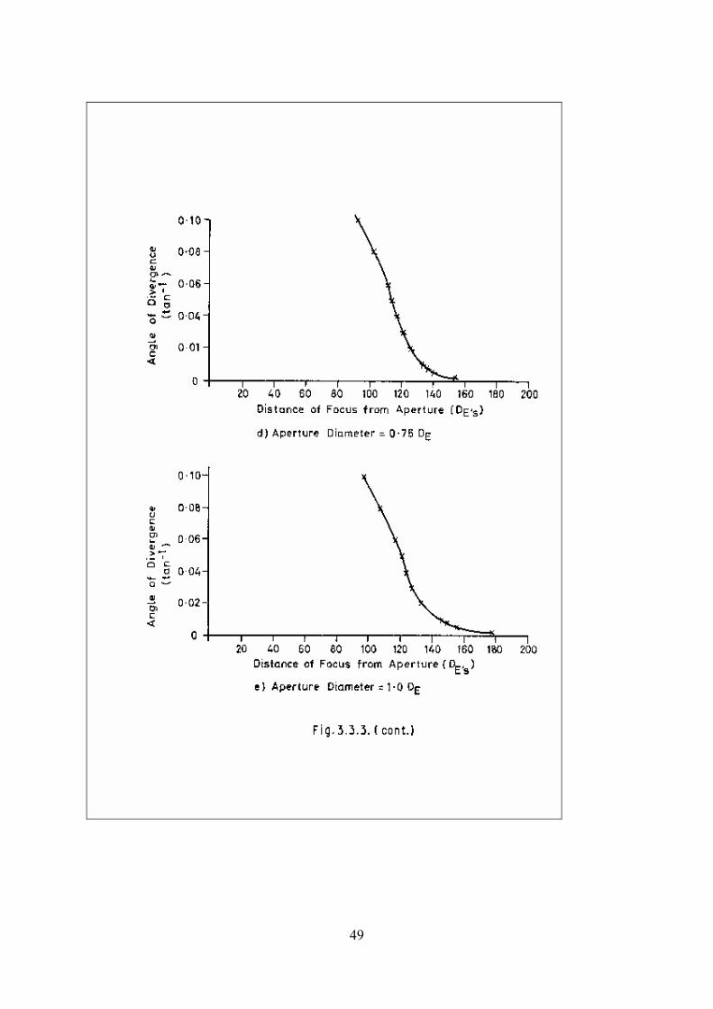
Rays originating from an axial point source 6 inches from the aperture were used for all the tests. The field inside the tube was nominally 3 KV/inch. The results are given in terms of' the diameter of the accelerating electrodes (DE ), which in fact was 4". Fig. 3.3.2 shows the foci of various rays from the point source against aperture size. The figures beside the graphs indicate tan-1 of the initial divergent angle. (These results and, those shown after, all assume a constant accelerating field over the whole region of focus. Neglecting the effects of the exit aperture, passage out from the accelerating field into a drift space would merely reduce the actual distance of focus, the qualitative picture remaining the same). Fig. 3.3.3 shows the variation of focus against initial angle for each of the apertures used. With the smaller apertures, the most divergent rays were lost to the boundaries. Taking as our measure of spherical aberration the difference in focus between the most and least divergent rays, it is obvious from Fig. 3.3.2 that for the particular conditions chosen there exists an aperture diameter between O.25DE and O.5DE for which this is a minimum (naturally dependent to some extent on the most divergent ray if none of the beam is to be lost). For a beam diverging at a maximum angle of tan-1 0.1, this is O.5DE; for tan-1 0.08 and all lesser angles it is approximately O.4DE. Computations with a different position of the point source produced similar results. Thus it is suggested that for this configuration generalisation is possible, i.e. for minimum spherical aberration the diameter of the initial aperture should be about a half that of the accelerating electrodes.

3. 4 The Aperture Lens

An approximation to the focal length of an aperture lens (a single circular aperture in a plane electrode separating two regions of different field is given by the formula

0

1 2

4fE E

φ=

− 3.1

where f is the focal length, 0φ is the potential on the electrode (with respect to zero energy particles), and E1 and E2 are the fields preceding and following the aperture. More accurately,

1 2

4 cfE E

φ=

− 3.2

where cφ is the potential at the centre of the aperture.

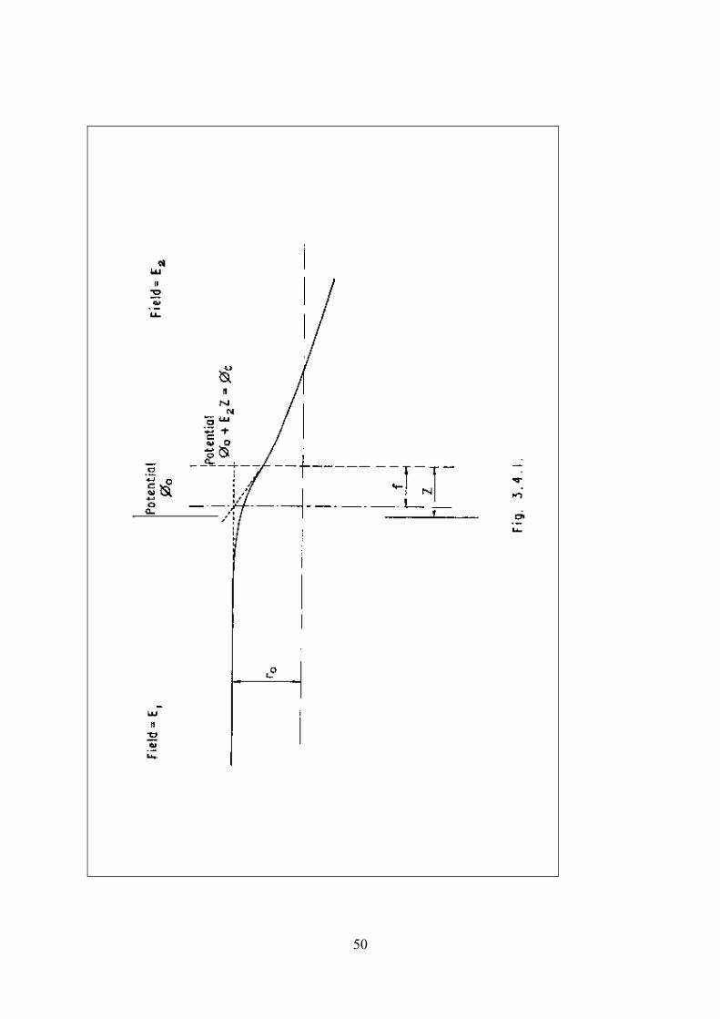
The focal length so defined is the axial distance between the intersection of the tangent to the particle path at 0 2 cE zφ φ+ = (Fig. 3.4.1) with the parallel incident ray, and with the axis. This definition is normally adopted since as constant fields (rather than constant potentials) are being considered, particle paths are parabolic before and after the lens action, and so the equations from which the lens parameters (as normally defined) may be calculated are complex, and in consequence rarely used. The equations are only valid if the fields on either side of the aperture are small compared to the ratio of the aperture potential to aperture diameter. (For a more detailed discussion on this topic, and the appropriate derivations see Reference [9]}

12

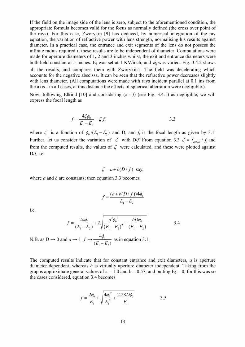
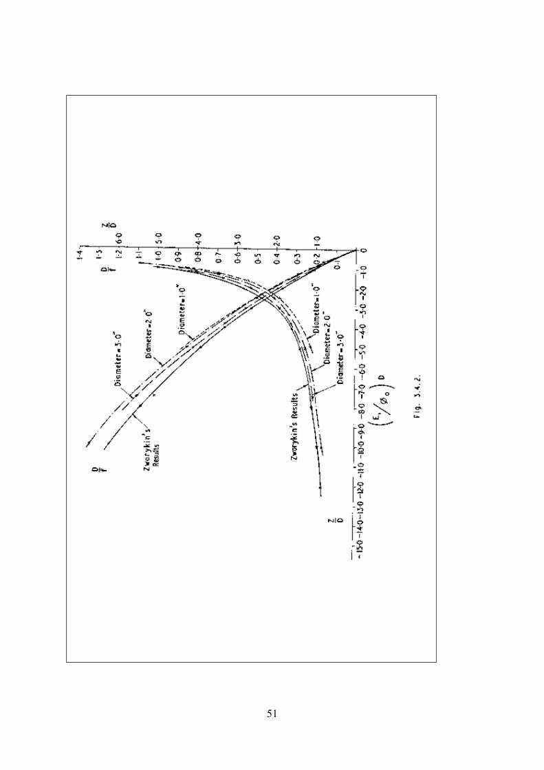
If the field on the image side of the lens is zero, subject to the aforementioned condition, the appropriate formula becomes valid for the focus as normally defined (the cross over point of the rays). For this case, Zworykin [9] has deduced, by numerical integration of the ray equation, the variation of refractive power with lens strength, normalising his results against diameter. In a practical case, the entrance and exit segments of the lens do not possess the infinite radius required if these results are to be independent of diameter. Computations were made for aperture diameters of 1, 2 and 3 inches whilst, the exit and entrance diameters were both held constant at 5 inches. E1 was set at 1 KV/inch, and 0φ was varied. Fig. 3.4.2 shows all the results, and compares them with Zworykin's. The field was decelerating which accounts for the negative abscissa. It can be seen that the refractive power decreases slightly with lens diameter. (All computations were made with rays incident parallel at 0.1 ins from the axis - in all cases, at this distance the effects of spherical aberration were negligible.) Now, following Elkind [10] and considering (z - f) (see Fig. 3.4.1) as negligible, we will express the focal length as

0

1 2

4tf f

E Eζφ ζ= =−

3.3

where ζ is a function of 0 1 2/( )E Eφ − and D, and ft is the focal length as given by 3.1. Further, let us consider the variation of ζ with D/f. From equation 3.3 /actual tf fζ = and from the computed results, the values of ζ were calculated, and these were plotted against D/f, i.e. ( / ) saya b D f ,ζ = +

where a and b are constants; then equation 3.3 becomes

0

1 2

( ( / ))4a b D ffE E

φ+=

−

i.e.

2 2

0 02

1 2 1 2 1 2

2 2( ) ( ) ( )

a a bDfE E E E E E

0φ φ= + +

− −φ−

3.4

N.B. as D → 0 and a → 1 0

1 2

4( )

fE E

φ→

− as in equation 3.1.

The computed results indicate that for constant entrance and exit diameters, a is aperture diameter dependent, whereas b is virtually aperture diameter independent. Taking from the graphs approximate general values of a = 1.0 and b = 0.57, and putting E2 = 0, for this was so the cases considered, equation 3.4 becomes

2

0 02

1 1 1

2 4 2.28DfE E E

0φ φ= + +

φ 3.5

13

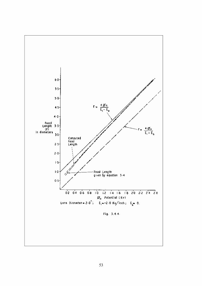
Using this formula, it was possible to predict over a wide range the focal lengths of other decelerating systems with field free image spaces, with an accuracy of better than 10% in all cases. Although the values a and b taken were approximate, the results predicted were far more accurate than those predicted by the simple formula (equations 3.2 and 3.1). An example is shown Fig.3.4.4 and Table 3.4.1. These results were for E1 = 2.0 KV /inch and D = 2.0 in. Equation 3.5 is thus presented as an empirical formula with which to predict the focal lengths of aperture lenses separating regions of constant decelerating field from field free image spaces to a greater accuracy than is possible by the lens formula alone.

4 Application to a Complete System Computations were made on the injector system of the Oxford Electrostatic Generator. [8,9]. A schematic of this is shown in Fig. 4.1. The configuration was considered in three sections:- a) The Ion Source Lens b) The Gap Lens c) The Accelerator Tube.

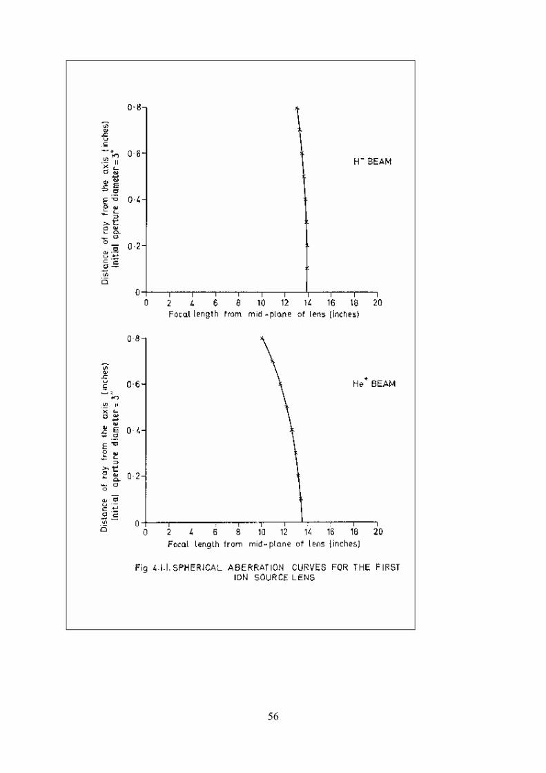
4. The Ion Source Lens

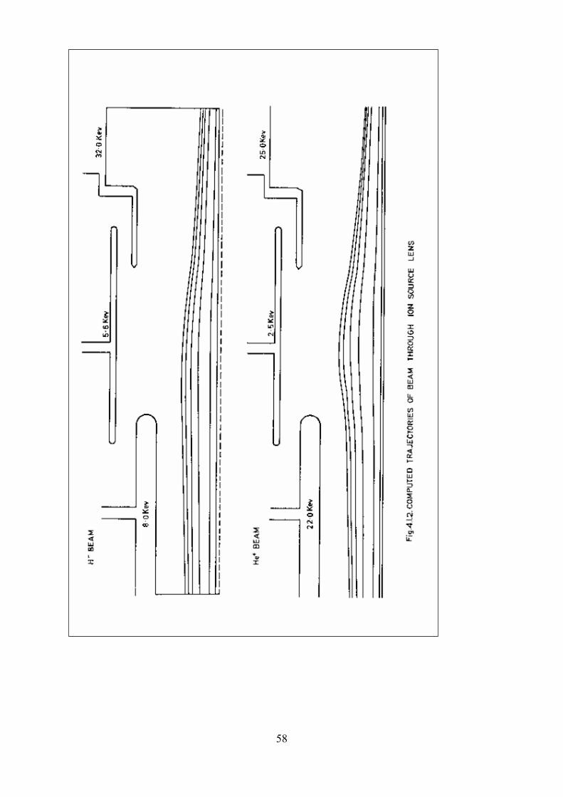
The fourth electrode of the ion source lens was held at the same potential as the third, so its focussing effect was negligible and thus only the first three were considered. The system was used to inject beams of both negative and positive ions, and there were thus two individual voltage configurations. Fig. 4.1.1 shows spherical aberration curves for the lens for these two conditions. The corresponding voltage configurations are shown in Fig. 4.1.2. The emittance of the ion source (assumed the same regardless of the type of ions) was known to approximate to a right ellipse with rmax = 1/16" and r'max = 1/40 radian. Several boundary rays were selected from this and an effective drift space assumed between the ion source and the first lens. In Fig. 4.1.2 the passage of these rays through the lens is shown for the two configurations. It was assumed that all other rays would lie within the envelope formed by these rays and their exact opposites (i.e. and i i ir r r ir′ ′= − = − )

4.2 The Gap Lens

The purpose of the gap lens was to match the potential of the particles emerging from the ion source lens with that at the beginning of the accelerator tube. In Fig. 4.2.1, the trajectories of the particles of the negative beam are shown, with the corresponding voltage configuration. A drift space was assumed between the lenses (Fig. 4.1). A more detailed investigation of gap lenses was performed, and has already been included. The beam was intended to focus in the aperture, which it does.

4.3 The Accelerator Tube

In Fig. 4.3.1, the trajectories of the same negative beam particles at the entrance to the accelerator tube are shown. This section continues straight on after the gap lens. Assuming that after the initial field disturbance at the entrance the particles are merely accelerated by a linear field (in fact, this was 24 KV/inch), then using the simple parabolic equations of motion their positions at any point thereafter can be calculated. In Fig. 4.1, the beam envelope through the initial focussing stages is shown. Again, further results on accelerator

14

tubes are shown later. These results show merely the performance of the actual configuration and experimentally optimised focussing potential in use.

5. Conclusion General consideration of the results indicates that, although many geometrically complicated systems have been designed, for a given lens strength (i.e. focal length), with regard to spherical aberration, these have little advantage over the simpler, more easily constructed systems. So long as the basic problem of inter-electrode breakdown is solved, then complex shaping of the electrodes is not worth the time and effort involved. The plain cylindrical einzel lens seems as adequate as any. A table of the collected results for the aberration coefficients determined is appended (Table 5.1). As stated previously, it is difficult to make any real comparisons between different types of lens, since to compare Cs in true fashion, the magnification of the lens must be taken into account. Even with lenses of the same type, in particular einzel lenses, it is difficult since there is a dependence on the focal length which Liebmanns [6] work suggests is not in fact linear; thus even the last column of the table is not a real comparison. In general however it may be said that the results follow the expected trends as indicated the individual sections. The program has shown its applicability to the analysis of particular lenses and some new results on the einzel, gap and aperture lenses have been presented. Further investigation of the last of these three lenses might be of use. Results of particular interest to accelerator tube designers have been obtained, and the properties of a complete system have also been computed, and it would seem that here, i.e. in predicting the action of a particular configuration, rather than in more generalised investigations, lies the most probable future application of the program.. In fact the program has already contributed to several specific projects, amongst these being the design of a novel configuration of electron gun for the Wantage Research Laboratory; to be used for paint curing purposes, and an analysis of the injector system of the Rutherford Laboratory's Proton Linear Accelerator. Present uses includes its exploitations a tool to investigate the effect of field emission on voltage breakdown in vacuum, and the prediction of the performance of an accelerator tube to be used at Tokio University.

Acknowledgements We wish to express our sincere thanks to Professor W. D. Allen for his many suggestions both on the computer experiments and in the compilation of this report. We are indebted to J. S. Hornsby now at the University College of North Wales, Bangor, for the provision of the first section of the program, and to N J Diserens for his early work on the program and subsequent helpful discussions. Finally we acknowledge the assistance of the Rutherford and Atlas Laboratories in the provision of computing facilities.

15

References [1] For a comprehensive bibliography, see P. Grivet, Electron Optics., Pergamon Press, 1965 [2] J S Hornsby, CERN 63-7, 1963 [3] L.S. Goddard, Proc. Phys. Soc. 56, 372, 1944 [4] E.G. Ramberg, J.App. Phys. 13, 582, 1942 [5] G.N. Plass, J.App. Phys. 13, 55 1942 [6] G. Liebmann, Proc. Phys, Soc. 213, 62, 1949. [7] A. Septier, CERN 60-39, 1960 [8] T R. Walsh, Plasma Physics 5, 17, 1963 [9] V.K. Zworykin, et. al., Electron Optics and the Electron Microscope, J Wiley’s, 1945 [10] M.M. Elkind, Rev. Sci. Inst. 24, 129, 1953. [11] F E Terman , Radio Engineers Handbook, McGraw Hill, 1943 [12] L.S. Goddard, Proc. Camb. Phil. Soc. 42, 106,1946 [13] P.P. Starling and J.V. Hoare, NIRL/M/58, 1963

16

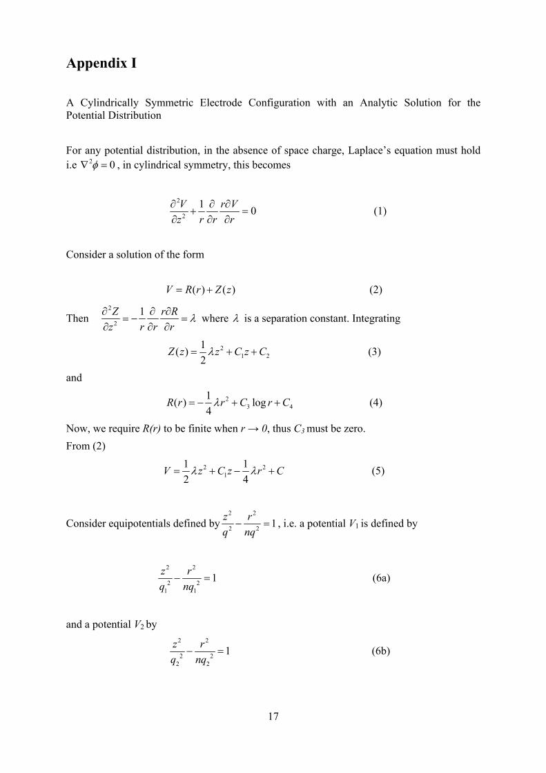
Appendix I A Cylindrically Symmetric Electrode Configuration with an Analytic Solution for the Potential Distribution For any potential distribution, in the absence of space charge, Laplace’s equation must hold i.e , in cylindrical symmetry, this becomes 2 0φ∇ =

2

2

1 0V r Vz r r r

∂ ∂ ∂+

∂ ∂ ∂= (1)

Consider a solution of the form (2) ( ) ( )V R r Z z= +

Then 2

2

1Z r Rz r r r

λ∂ ∂ ∂= − =

∂ ∂ ∂ where λ is a separation constant. Integrating

21

1( )2 2Z z z C zλ= + +C (3)

and

23

1( ) log4 4R r r C rλ= − + +C (4)

Now, we require R(r) to be finite when r → 0, thus C3 must be zero. From (2)

21

1 12 4

V z C z rλ λ= + − +2 C (5)

Consider equipotentials defined by2 2

2 2 1z rq nq

− = , i.e. a potential V1 is defined by

2 2

2 21 1

1z rq nq

− = (6a)

and a potential V2 by

2 2

2 22 2

1z rq nq

− = (6b)

17

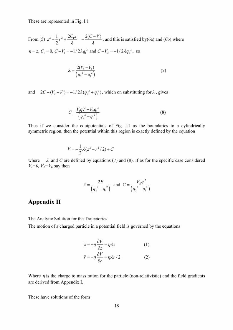
These are represented in Fig. I.1

From (5) 2 2 121 2(2

C z C Vz rλ λ

−− + = −

)

2

, and this is satisfied by(6a) and (6b) where

2 21 1 1 2, 0, 1/ 2 and 1/ 2n z C C V q C V qλ λ= = − = − − = − , so

( )

2 12 2

2 1

2( )V Vq q

λ −=

− (7)

and , which on substituting for2 22 1 2 12 ( ) 1/ 2 (C V V q qλ− + = − + ) λ , gives

( )

2 21 2 2 1

2 22 1

V q V qCq q

−=

− (8)

Thus if we consider the equipotentials of Fig. I.1 as the boundaries to a cylindrically symmetric region, then the potential within this region is exactly defined by the equation

2 21 ( / 2)2

rλV z C= − − +

where λ and C are defined by equations (7) and (8). If as for the specific case considered V1=0, V2=VE say then

( ) ( )

21

2 2 2 22 1 2 1

2 and EV qE Cq q q q

λ −= =

− −

Appendix II The Analytic Solution for the Trajectories The motion of a charged particle in a potential field is governed by the equations

(1)

/ 2 (2)

Vz zzVr rr

η ηλ

η ηλ

∂= − =

∂∂

= − =∂

Where η is the charge to mass ration for the particle (non-relativistic) and the field gradients are derived from Appendix I. These have solutions of the form

18

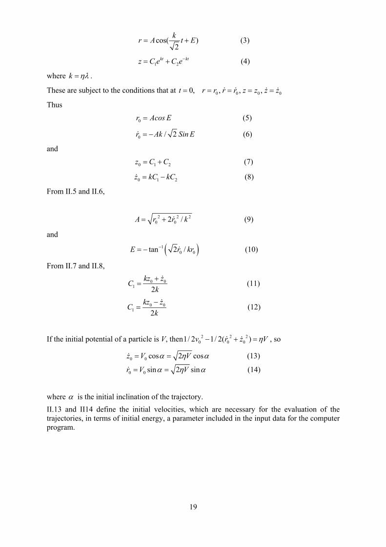
cos( )2

kr A t E= + (3)

1 2kt ktz C e C e−= + (4)

where k ηλ= .

These are subject to the conditions that at t r 0 0 00, , , ,r r r z z z 0z= = = = =

Thus

(5) 0r Acos= E

0 / 2r Ak Sin= − E

2

2

(6)

and

(7) 0 1z C C= +

(8) 0 1z kC kC= −

From II.5 and II.6,

2 20 02 / 2A r r k= + (9)

and

( )10 0tan 2 /E r−= − kr (10)

From II.7 and II.8,

0 01 2

kz zCk+

= (11)

01 2

kz zCk−

= 0

V

(12)

If the initial potential of a particle is V, then1/ 2 2 20 0 02 1/ 2( )v r z η− + = , so

0 0

0 0

cos 2 cos (13)

sin 2 sin (14)

z V V

r V V

α η α

α η α

= =

= =

where α is the initial inclination of the trajectory. II.13 and II14 define the initial velocities, which are necessary for the evaluation of the trajectories, in terms of initial energy, a parameter included in the input data for the computer program.

19

Figures

20

21

22

23

24

25

26

27

28

29

30

31

32

33

34

35

36

37

38

39

40

41

42

43

44

45

46

47

48

49

50

51

52

53

54

55

56

57

58

59

60