the path of the ultimate loss ratio estimate

The Path of the Ult imate Loss Ratio Est imate

Michae l G. Wacek , FCAS, M A A A

Abstract This paper presents a framework for stochastically modeling the path of the ultimate loss ratio estimate through time from the inception of exposure to the payment of all claims. The framework is illustrated using Hayne's lognormai loss development model, but the approach can be used with other stochastic loss development models. The behavior of chain ladder and Bornhuetter-Ferguson estimates consistent with the assumptions of Hayne's model is examined. The general framework has application to the quantification of the uncertainty' in loss ratio estimates used in reserving and pricing as well as to the evaluation of risk-based capital requirements for solvency and underwriting analysis.

Keywords: Stochastic model, diffusion process, loss development, loss ratio estimation, lognormal, Student's l, log t, parameter uncertainty"

1. I N T R O D U C T I O N

Ultimate loss ratio estimates change over time. The initial loss ratio estimate that emerges

from the pricing analysis for a tranche of policies soon gives way to a new estimate as time

passes and claims begin to emerge (or not). By the time all claims have been paid, the loss

ratio is likely to have been re-estimated many times. The focus of this paper is on how to

model the future revisions of these ultimate loss ratio estimates. We illustrate the approach

using loss ratio estimates based on chain ladder and Bornhuetter-Ferguson methods

underpinned by a simple stochastic model described by Hayne [1].

There appears to be little, if any, actuarial literature on the subject of behavior of a

ultimate loss ratio estimate behveen the time when it is made and the time when its final value

becomes known, i.e., the point at which all claims have been paid. Various authors have

sought to address uncertainty in the ultimate loss ratio estimate, but generally from the

perspective of a single point in time.

For example, Hayne [1] proposed a lognormal model of loss development that supports

the construction of confidence intervals around the ultimate loss ratio estimate ~. Kelly [2]

and Kreps [3] also used a lognormal framework to explore issues of parameter estimation

and parameter uncertainty, respectively. Hodes, Feldblum and Blumsohn [4] used a slightly

different lognormal development model to quantify the uncertainty in workers

compensation reserves. Mack, Venter and Zehnwirth have all written extensively about

1 Conscious that the confidence intervals he derived were dependent on the lognormal model being the correct choice, he cautiously described his results as providing a "range of reasonableness."

339

The Path of the Ultimate Loss Ratio Estimate

stochastic modeling of the loss development process:. Others, including Van Kampen [11],

Wacek [12] and the American Academy of Actuaries Property & Casualty Risk-Based Capital

Task Force [13], have sought to quantify the uncertainty in the ultimate loss ratio estimate

used in pricing and reserving applications direcdy, without reference to the loss development

process. The question on which all of these authors focused their attention is the potential

variation in the final loss ratio at ultimate compared to the current ultimate loss ratio

estimate, with no reference to how the ultimate loss ratio estimate might vary at intermediate

points in time.

In contrast, in his acclaimed paper on solvemy measurement Butsic [14] observed that

loss estimates change in their march through time. He recognized that they, like stock

prices, are governed by a diffusion process, a type of continuous stochastic process with a

time-dependent probability structure. However, he did not propose a model of this

stochastic process.

How ultimate loss ratio estimates change in the future depends in part on the method

used to make the estimates. In this paper we assume that loss ratio estimates are derived

from a consistently applied estimation process with minimal subjective overriding of the

indicated result. We model the behavior of loss ratio estimates using stochastic versions of

two loss development methods: the chain ladder method and the Bornhuetter-Ferguson

method, both using paid development data. To model chain ladder estimates, we combine

Hayne's and Butsic's ideas to synthesize a lognormal diffusion model for the path of the

ultimate loss ratio. Then we adapt that model to the Bornhuetter-Ferguson method.

This conceptual framework, which could easily be adapted to handle other loss

development models, provides actuaries with the means to give their clients more

information about how much their loss ratio or reserve estimates may fluctuate from period

to period. As such, it can be a useful tool for managing expectations about the variability of

loss reserve estimates. It also has potential application in a number of other areas of

actuarial analysis, as we will discuss later.

1.1 O r g a n i z a t i o n o f t h e P a p e r

The paper comprises six sections, the first being this introduction. In Section 2 we

outline Hayne's lognormal model of chain ladder loss development and illustrate its

application using industry Private Passenger Auto Liability data from the 2004 Schedule P.

We illustrate the main benefit of a stochastic model for loss development, namely, the ability

2 For example, see Mack 151, 16], Venter 17], 18] and Zehnwirth [9], [10] (the last co-authored with Barnett).

340 Casua l t y Actuar ia l Socie ty Forum, W i n t e r 2 0 0 7


to measure the uncertainty in loss development factors and in the ultimate loss ratio

estimate.

In Section 3 we discuss the effect of future loss emergence on future ultimate loss ratio

estimates. We show how to use information implicit in Hayne's model to determine the

distribution of future estimates derived from our stochastic versions of the chain ladder and

Bornhuetter-Ferguson methods, with particular attention to the loss ratio estimate one year

out. We again use industry Private Passenger Auto Liability data to illustrate the process.

In Section 4 we adjust Hayne's model to allow for parameter uncertainty, and illustrate

the effect. Because the adjusted distribution does not have the multiplicative properties of

the lognormal, we illustrate the use of Monte Carlo simulation to model the distribution of

future ultimate loss ratio estimates.

In Section 5 we conclude with an outline of potential applications of the framework for

future ultimate loss ratio estimates in loss reserving and risk-based capital applications.

2. HAYNE'S L OGNORMAL LOSS D E V E L O P M E N T M O D E L

Hayne presented two models of chain ladder loss development: one that assumed that

development is independent from one period to the next, and a second one that relaxed the

independence assumption. We will adopt the first model (and henceforth refer to it simply

as "Hayne's model"). Kelly [2] argued that independence is more plausible for paid loss

development than for case incurred development. Therefore, we will use paid losses as the

basis of our framework.

Hayne's model is quite simple. He assumed that age-to-age development factors are

lognormally distributed. The product of independent lognormal random variables is also

lognormal, which implies that age-to-ultimate loss development factors are lognormal.

Because the product of a constant and a lognormal random variable is lognormal, if we are

given the cumulative paid loss ratio at any age and the estimated parameters of the matching

age-to-ultimate factor, we can determine the parameter estimates of the ultimate loss ratio.

Using these parameters we can estimate the expected loss ratio (which we will take as the

"best" estimate) as well as confidence intervals around that estimate.

The lognormal parameters g. and ~ of the age-to-age factors can be estimated by a

variety of methods. Hayne used (and we also prefer) the unbiased estimators 1 n : n - 2

1,__~l =n,__ ~ , ~ ~1----[ f°r t* and ° - ' respectively' where ~;=n,= y' /n(:c ) and s 2 = y ( 3 " - Y )

Casua l t y Ac tua r i a l Socie ty Forum, W i n t e r 2 0 0 7 341

The Path of the Ultimate Loss RaHo Estimate

"\~1~ "X'2' "X'3)"') ~'n

estimator.

are the, observed age-to-age factors 3. is also a m a ~ m u m likelihood

2.1 IUustration of Model Parameter Estimation

We illustrate the parameter estimation for Hayne's model using the real loss

development data presented in Exhibits 1 and 2. Exhibit 1 shows industry aggregate

Schedule P net paid loss development data for Private Passenger Auto Liability- for accident

years 1995 through 2004 from the 2004 Annual Statement 4 together with ~ e associated paid

loss age-to-age development factors. The paid loss ratios at age one year are also included in

the development factor exhibit. Exhibit 2 shows the natural logarithms of the age-to-age

factors and the age one year paid loss ratios. The rows labeled "Mean" and "S.D." in

Exhibit 2 show the unbiased estimators for p. and e , respectively, given the data in the

body of the column 5.

For example, in Exhibit 2 the mean and standard deviation of the natural logarithms of

the observed age 1 to 2 development factors are 0.569 and 0.016, respectively. I f we set

bt = 0.569 and a = 0.0166, these parameter estimates for prospective age 1 to~2 development

imply a lognormal mean, defined as E(x) = e ~+°s*~ , of 1.767, which matches the mean loss

development factor calculated by the traditional method in Exhibit 1. The same is true for

all of the other age-to-age factors. Similarly, the parameter estimates for the age one paid

loss ratio are -1.246 and 0.069 for ~t and or, respectively, which imply a lognormal mean of

28.8%. This, too, matches the mean age one paid loss ratio shown in Exhibit 1.

The parameter estimates for the prospective age-to-age factors can 'be combined using

the multiplicative property of lognormal distributions to determine parameter estimates for

prospective age-to-ultimate factors. The product of n lognormal random variables with

respective parameter sets (~q,%), (~z,a2) , (~t3,a3),..., (bt,,,¢~,) is a lognormal random I

variable with parameters ~ = ~, and ~ = o, . For example, treating age 10 as

ultimate, in Exhibit 2 the ~. parameter estimate for the age 7 to ultimate development factor

is the sum of the mean age-to-age factors forages 7 to 8, 8 to 9 and 9 to 10:0.005 + 0.003 +

3 We used unweightcd estimators throughout this paper. For formulas for estimators using unequal weights for the observations, see Section 5.5 of [12].

4 Source: Highline Data LLC as reported in the statutory filings (OneSource). 5 Note that the standard deviation for the age 9 to 10 development factor, which is undefined, 'has been

selected to be equal to that of the age 8 to 9 development factor in both Exhibit 1 and Exhibit 2. 6 These parameters define the lognormal distribution that best fits the data, using unbiasedness as the criterion

for "best." However, there is uncertain~" about whether those parameters are correct. We address the issue of parameter uncertainty later in the paper.

3 4 2 C a s u a l t y A c t u a r i a l Soc i e ty Forum, W i n t e r 2 0 0 7

The Path, of the Ultimate Loss Ratio Estimate

0.001 = 0.009. The corresponding o parameter is the square root of the sum of the

variances of the same age-to-age factors: ~/0.0002 + 0 .0012 + 0 .0012 = 0.001. Note that the

lognormal means (labeled "LN Fit LDFs" in Exhibit 2) implied by these age-to-ultimate

parameters match the age-to-ultimate development factors shown in Exhibit 1.

The ultimate chain ladder loss ratio estimates indicated by this analysis as of the end of

2004 for accident years 1995 through 2004 are summarized in Exhibit 3. In this example,

the lognormal loss development model produces the same loss ratio estimates as the

traditional deterministic chain ladder loss development method. I f we were interested only

in these mean estimates, the traditional approach would suffice. However, we also want to

measure the uncertainty" in the loss ratio estimates, and for that purpose the richer lognormal

model is superior.

2.2 Measurement of Loss Development Uncertainty

If we assume ~t = ~ and G = s based on the data for each age-to-age development period,

we can calculate the lower and upper bounds of a two-sided 95% confidence intetaTal for

prospective age-to-age factors as e J'-'\-*(97's%)* and e '}+N-~(97's'~'')'s, respectively, where

N-1(97.5%) is the value of the standard normal cdf corresponding to a cumulative

probability" of 97.5% v. Similarly, using the parameter estimates for the age-to-ultimate

factors we can also determine confidence intervals for age-to-ultimate factors. We have

tabulated these 95% confidence intervals based on the industry. Private Passenger Auto

Liabilit T Schedule P data as of the end of 2004 in Exhibit 48.

Exhibit 4 indicates that the age 1 to 2 development factor, which has an estimated mean

of 1.767, should fall within a range of 1.710 to 1.824 95% of the time. The age 1 to ultimate

development factor, which has an estimated mean of 2.508, can be expected to fall within a

range of 2.423 to 2.595 95% of the time. Given the accident year 2004 paid loss ratio of

26.6% at age 1, these confidence intervals imply a paid loss ratio range at age 2 of 45.5% to

48.5% (47.0% + 1.5%) and an ultimate loss ratio range of 64.4% to 69.0% (66.7% + 2.3%) 9.

As we would expect, the development factors for more mature accident )'ears have tighter

confidence intervals. For example, the age 5 to 6 factor, which in a year end 2004 analysis

v N-I (97.5%) is replicated in Excel by NORAISIN[ r(0.975). Bear in mind that these confidence intervals, are premised on the parameter estimates being correct and are narrower than confidence inte~'als that incorporate parameter uncertainty.

9 While the lognormal is a skewed distribution, the skewness is imperceptible for small values of G and the confidence intervals are, for most practical pt4rposes, symmetrical. In this example with G = 0.016 the skewness coefficient is 0.05. In contrast, m the case ofo = 1 it ts 6.18.

C a s u a l t y A c t u a r i a l S o c i e t y Forum, W i n t e r 2 0 0 7 3 4 3


would be applicable to accident year 2000, has an estimated mean of 1.020 and a 95%

confidence range of 1.018 to 1.022. That implies that, 95% of the time, the accident year

2000 paid loss ratio of 76.7% as of the end of 2004 will develop to a paid loss ratio of 78.1%

to 78.4% by the end of 2005, a range of 0.3 points. The 95% confidence interval for the age

5 to ultimate factor, which has an estimated mean of 1.039, is a range of 1.034 to 1.043.

That implies an ultimate loss ratio range of 79.3% to 80.0%, or 0.7 points.

All of these development factor, loss ratio and confidence interval estimates are as of the

end of 2004. They are all subject to change as new information in the form'of actual future

loss emergence becomes available. In the next section we will show how to use information

implicit in Hayne's approach to model the effect of future loss emergence on these

estimates.

3. A M O D E L FOR F U T U R E ULTIMATE LOSS RATIO ESTIMATES

Any estimate of the ultimate loss ratio for a particular accident year is quickly made

obsolete by subsequent actual loss emergence. Because of this rapid obsolescence, the

ultimate loss ratio must be re-estimated periodically in light of the loss development in the

period since the previous evaluation. That loss development affects the new estimate in two

ways.

3.1 Sources of Variation in Future Loss Ratio Estimates

First, the actual accident year loss emergence replaces the expected emergence in the loss

ratio projection. For example, in Exhibit 3 the Private Passenger Auto Liability accident year

2004 ultimate loss ratio of 66.7%, estimated as of the end of 2004, was determined by

applying an age-to-ultimate factor of 2.508 to the paid loss ratio of 26.6%. That age-to-

ultimate factor reflected an exT~ected age 1 to 2 development factor of 1.767 combined with an

age 2 to ultimate factor of 1.420.

It is likely that actual age 1 to 2 loss development will vat 3, from the expected. If, for

example, the actual accident year 2004 emergence during 2005 (from age 1 to 2) corresponds

to a development factor of 1.75, then in the ultimate loss ratio analysis conducted at the end

of 2005 this actual development factor will replace the expected development factor of

1.767. If the age 2 to ultimate factor remains unchanged at 1.420, the revised chain ladder

estimate of the ultimate loss ratio will become 26.6% x 1.75 x 1.42 = 66.1%. The revised

344 Casualty Actuarial Society Forum, Winter 2007

The Path,of the Ultimate Loss Ratio Estimate

Bornhuetter-Ferguson loss ratio estimate will become 26.6%,.x:.(1.75 - 1.767) + 26.6% x

1.767 x 1.42 = 66.1% 1°.

O f course, loss emergence with respect to older accident years might cause a revision in

the prospective age 2 to ultimate factor. This potential for tail factor revision is a second

source of uncertainty. For example, suppose the actual age 2 to 3 development on accident

year 2003 during 2005 corresponds to a factor of 1.210. I f that factor is averaged with the

previous eight-point mean of 1.198 determined in Exhibit 1 (using loss development data

through 2004), the result is a revised age 2 to 3 development factor of 1.199. Assuming the

same process is repeated for the other development periods, a revised age 2 to ultimate

factor will be obtained. I f the resulting age 2 to ultimate factor is 1.425, the revised chain

ladder ultimate loss ratio estimate is given by 26.6% x 1.75 x 1.425 = 66.3%, a reduction of

0.4% from the year end 2004 ultimate loss ratio estimate of 66.7%. The revised

Bornhuetter-Ferguson estimate in this case is given by 26.6% x (1.75 - 1.767) + 26.6% x

1.767 x 1.425 = 66.5%.

The foregoing is an illustration of just one scenario of the loss development that might

occur in 2005 and its effect on the ultimate loss ratio estimate. We can use information

developed in Hayne's framework to model these two effects generally.

3.2 M o d e l i n g t h e F i r s t S o u r c e o f V a r i a t i o n - A c c i d e n t Y e a r D e v e l o p m e n t

The first effect is captured by the lognormal random variable estimated for the next year

of development with respect to the adcident year under review. For example, for accident

year 2004, which at. the end of 2004 is age 1, the log, normal distribution with i ~ = 0.569 and

o = 0.016 models age 1 to 2 paid development. Then, since the age 1 paid loss ratio is

26.6%, the paid loss ratio distributioti at age 2 is lognormal with parameters bt = / n 26.6% +

0.569 = - 0 J 5 6 and o = 0.016, implying a mean of'47.0%.

I f the mean age 2 to ultimate factor (the tail factor) of 1.42 does not change, then the

distribution of the revised chain ladder ultimate loss ratio estimate at age 2 (i.e., one ),ear out)

has lognormal parameters ~ = /n 26.6% + 0.569 + /n 1.42 = -0.406 and c = 0.016. The

random variable for this chain ladder estimate xc~ can be expressed as a function of the

paid loss ratio random variable xp and:the expected value of the mean tail factor: I

Xcl = xp " E ( tai/) (3.1)

m Assume the Bornhuetter-Ferguson expected loss ratio is 66.7%. In general, we will assume the Bomhuetter- Ferguson expected loss ratio for each accident year as of the end of 2004 is equal to the chain ladder ultimate shown in Exhibit 3, allowing us to treat the year end 2004 loss ratio estimates as identical from both methods.

C a s u a l t y A c t u a r i a l S o c i e t y F o r u m , W i n t e r 2 0 0 7 3 4 5


The random variable xm:,. for the comparable Bornhuetter-FergUson.estimate is a shifted

version of the random variable for the age 2 paid loss ratio:

x m- = xp - E( . , :p ) + E ( x p ) . E ( t a i / ) (3.2)

As defined by Formulas 3.1 and 3.2, both Xcl and xnF reflect the uncertain impact of

accident year 2004 development during 2005 on the updated ultimate loss ratio estimate that

will be made at the end of 2005, but do not reflect the potential impact of tail factor revision.

3.3 M o d e l i n g t h e S e c o n d S o u r c e o f V a r i a t i o n - T a i l F a c t o r R e v i s i o n

The second effect, due to tail factor revision, is captured by measuring the effect of the

lognormal loss development modeled for the next year on the existing mean age-to-age and

age-to-ultimate factors. For example, the mean age 2 to 3 development factor shown in

Exhibit 1 is 1.198. This is a mean of eight data points. What will b e the effect on the mean

of adding a ninth data point (representing 2005 development on accident year 2003), given

that it will arise from a lognormal distribution with parameters ta = 0.18l and o = 0.005

(and mean of 1.198)? The uncertain ninth data point will contr ibute 'one-ninfh weight to the

revised mean age-to-age factor. There is no uncertainty about the existing mean age 2 to 3

factor - it is a constant. Therefore, the o parameter of the distribution of the revised mean

age 2 to 3 factor one year out, given an additional year of actual development, is given by

~/(9-0)2 +(9 .0 .005)2 =0.001. T h e ~ parameter is given by /t11.198-0.5-0.0012 =0.181.

We can use the same process to estimate ~ and cr parameters for the comparable

distributions of mean age-to-age factors one year out for all such factors comprising the

development tail". We can then combine the revised mean age-to-age factor parameters to

determine the parameters of the revised mean age-to-ultimate factor distributions. See

Exhibit 5 for a tabulation of the parameters of these revised mean age-to-age and age-to-

ultimate distributions for all ages. The a of the distributions of revised factors for age 3 to

4 and beyond is less than 0.0005 (and thus displayed as 0.000 in Exhibit 5), indicating that

for Private Passenger Auto Liability, the uncertainty arising from the potential for tail factor

revision is very small. This is confirmed by the veq, narrow confidences intervals.

t l Bear in mind that these parameters refer to distributions of the mean age-to-age development factor one year out and not to distributions of the development factor itself. We are interested in the distribution of the mean development factor because changes in the mean directl)7 affect the ultimate loss ratio estimate (which is also a mean).

3 4 6 C a s u a l t y A c t u a r i a l Soc i e ty F o r u m , W i n t e r 2 0 0 7

The Path. of the Ultimate Loss Ratio Estimate

3.4 Modeling the Revised Loss R a t i o E s t i m a t e O n e Y e a r O u t

We can now combine these two effects to determine the distribution of the revised

ultimate loss ratio estimate that will be determined in one year's time based on the updated

loss development experience that will then be available.

To determine the distribution of the revised chain ladder estimate, we start with the actual

accident year paid loss ratio, which we then multiply by the lognormal random variables for

l) the age-to-age factor for the next year of development (obtaining the random variable xp

of the paid loss .ratio one year out) and 2) the revised age-to-ultimate factor beyond the next

year of development. Using accident year 2004 as an example, as of the end of 2004 the

ultimate loss ratio estimate is 66.7%, which has been determined by multiplying the paid loss

ratio of 26.6% first by an age 1 to 2 factor of 1.767 and then by an age 2 to ultimate factor of

1.420. In order to model the ultimate loss ratio estimate one year later, at the end of 2005,

we replace the constant age 1 to 2 factor of 1.767 with the lognormal random variable with

parameters I~1 = 0:569 and o I = 0.016. In addition, we replace the constant age-to-ultimate

factor of 1.420 with the lognormal random variable with parameters bt2 = 0.350 and 02 =

0.001. The expected values of these two lognormal random variables are 1.767 and 1.420,

respectively. The product of the paid loss ratio (a constant) and these two lognormal

random variables is lognormal with parameters p. = / n P + bt~ + g-2 and o = ~ 7 + 022 , where

P represents the actual paid loss ratio at the end of 2004, which in this example, implies I* =

-1.325 + 0.569 + 0.350 = -0.406 and o = ~/1.0162 + 0.0012 = 0.017.

Generally, we can express the random variable XcL as the product of the two lognormal

random variables x I, and tai/, representing the paid loss ratio one year out and the mean tail

factor:

x c l = x l , . tail (3.3)

Now we are in a position to determine confidence intervals for the revised chain ladder

ultimate loss ratio estimate at the end of 2005. The endpoints of the two-sided 95% la+N-I (97.5%p~ confidence interval are given by e "-'\-~(vTs%;° and e , which imply an estimated

loss ratio range one year out for accident year 2004 of 64.5% to 68.8%, or approximately

66.7% + 2.1%. Confidence intervals for ultimate loss ratio estimates one year out for the

other accident years can be estimated in the same way, and are tabulated together with those

for accident year 2004 in Exhibit 6.

To determine the distribution of tl~e comparable revised Bornhuetter-Ferguson estimate,

we replace the constant E( ta i l ) in Formula 3.2 with the random variable tail'.

C a s u a l t y A c t u a r i a l S o c i e t y F o r u m , W i n t e r 2 0 0 7 3 4 7


x~r = xp - E ( x v ) + E ( x p ) . tail (3.4)

We can also determine confidence intervals for the revised Bornhuetter-Ferguson loss

ratio estimate at the end of 2005. However, because the sum of two lognormal random

variables, in this case xp and tail, is not expressible in closed distributional form, the

confidence intervals must be estimated using Monte Carlo simulation. The results of a

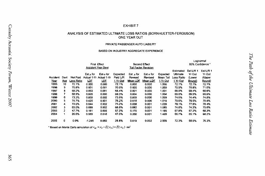
simulation involving 10,000 trials are shown in Exhibit 7. For each of the trials we randomly

selected observations from the distributions of x v and tail, assuming independence, and

combined them according to Formula 3.4 to arrive at a simulated Bomhuetter-Ferguson

estimate. After tabulating the results of 10,000 such trials, we determined the lower and

upper bounds of the 95% confidence interval of the loss ratio estimate by identifying the 2.5

percentile and the 97.5 percentile of the trial values. Not surprisingly, the 95% confidence

intervals for the revised Bornhuetter-Ferguson estimates are narrower in every case than the

revised chain ladder estimates.

3.5 M o d e l i n g the R ev i s ed Loss Ratio E s t i m a t e - Other T i m e H o r i z o n s

We can extend this process to longer time horizons and determine the distribution of the

ultimate loss ratio estimate two years out, three years out and so on, until the time horizon

encompasses the point when all claims are expected to have been setded. The modeling is

conducted in essentially the same way as for the one year time horizon. For example, in the

case of a two-year horizon, the first source of uncertainty (accident year development) is

modeled using the distribution of the agej t o / + 2 development factor, where j is the age in

years of the accident year under review. The second source of uncertainty (potential tail

factor revision) is modeled by reference to the potential effect of two additional

development data points on the mean tail factor for a g e j + 2 to ultimate development. The

analysis of a three year time horizon focuses on accident year development from age j

to j + 3 and the tail factor from j + 3 to ultimate, but is otherwise identical to that for the

one year and two year time horizons. The analysis of the ultimate loss ratio estimate at

points further in the future proceeds in the same way.

Alternatively, we can model the path of the ultimate loss ratio estimate as a succession of

annual revaluations. Exhibit 8 illustrates this by plotting the results of one simulation of the

path of the accident year 2004 loss ratio estimates through time for estimates determined

from both chain ladder and Bornhuetter-Ferguson methods. It represents just one path

among many possibilities. The simulation was performed from the vantage point of the end

of 2004. As such it incorporates everything we know about actual loss development through

that time as well as what we can infer about the structure of future development. We started

348 C a s u a l t y Ac tua r i a l Soc ie ty F o r u m , W i n t e r 2 0 0 7


with the accident year 2004 loss ratio estimate as of the end of 2004, which was 66.7%.

Then, based on one random simulation of loss development during calendar year 2005, we

made new chain ladder and Bornhuetter-Ferguson estimates of the ultimate loss ratio as of

the end of 2005. We repeated the process for calendar years 2006 through 2013 using the

simulated cumulative loss development through each valuation date. Exhibit 8 is a plot of

the results. A complete description of the probability structure of the path can be built up

from a simulation involving a large number of random trials, or in the chain ladder case,

directly from the properties of the lognormal distribution.

In practice, there might not be much benefit in determining the distribution of the chain

ladder ultimate loss ratio estimate for time horizons between one },ear and the ultimate

horizon (when all claims have been settled), at least for Private Passenger Auto Liabilit3/2.

We see this in Exhibit: 9, the top half of which compares the 95% confidence intervals for

the accident year 1995 through 2004 chain ladder loss ratio estimates one year out with

confidence intervals for the accident year loss ratio estimates over the ultimate time horizon.

I f we contrast the 95% confidence interval for accident year 2004 for the one year horizon

with the 95% confidence interval for the chain ladder loss ratio estimate over the ultimate

time horizon, we can see that the contribution from the out years is dwarfed by the

contribution from the next twelve months. The 95% confidence interval for the ultimate

time horizon indicates a range for the accident year 2004 loss ratio of 66.7%_+ 2.3%, which

is barely wider than the range for just one year out. This is true not only for accident year

2004, but also holds for accident years 1995 through 2003.

For example, the accident year 2003 confidence interval of approximately 67.8% + 0.7%

for a one year time horizon is almost as wide as that for the time horizon to ultimate of

67.8%_+0.8%. For all of the older accident years, the first year of future development

accounts for more than half of the variation associated with the ultimate time horizon.

This phenomenon is not confined to loss ratio estimates over short vs. longer time

horizons. The same effect is also seen in other situations not related to insurance, where

variability" is a function of time. For example, given the common assumption that future

stock price movements are lognormally distributed and independent, the 95% confidence

interval for a stock price one year out, given constant annualized volatilit3T of o = 20% and an

expected value of $66.70, is $45.07 to $98.71, a range of $53.64. Assuming the same

expected value of $66.70, the 95% confidence interval for the stock price two years out is

$38.22 to $116.11, a range of $77.80. The confidence interval range for the one-year time

12 There might be value in doing so for other lines that display more loss development variability.

Casualty Actuarial Society Forum, Winter 2007 349


horizon stock price is 69% of the price range for the two-year time horizon. The reason for

the disproportionate impact of the first period is that the confidence interval is not a linear

function of a but rather of off7, where t represents the time lag in years. In the case of

chain ladder ultimate loss ratio estimation, where the age-to-age a typically declines as the

accident year ages, this effect can be even more pronounced.

Turning now to the Bornhuetter-Ferguson estimates, which are inherently less variable,

the effect is smaller but still evident. The bot tom half of Exhibit 9 compares the 95%

confidence intervals for accident year 1995 through 2005 loss ratio estimates one ),ear out

with the confidence intervals for the loss ratio estimates over the ultimate time horizon. In

the Private Passenger Auto Liability example considered here, the 95% confidence interval

for the accident year 2004 loss ratio estimate is appro:dmately 66.7%_ 1.6%, which is about

two-thirds of the range of the confidence interval for estimates at the ultimate time horizon.

For all of the older accident years, as in the case of the chain ladder estimates, the first ),ear

of future development accounts for more than half of the variation associated with the

ultimate time horizon.

3 .6 M o d e l i n g t h e L o s s R a t i o E s t i m a t e a t Inception Up to this point we have focused on modeling the distribution of the ultimate loss ratio

after losses have begun to emerge. However, there is no reason why we cannot extend

essentially the same procedure backward to the inception of loss exposure at age 0. Indeed,

the benefit of doing so is that we can obtain a complete model of the path of the ultimate

loss ratio from inception to ultimate.

The main difference in the procedure is that the lognormal model for loss emergence

between age 0 and 1 describes the behavior of the paid loss ratio rather than an age-to-age

factor. The rest of the analysis is merely an application of Formula 3.3.

For example, assume for the sake of illustration that the age 1 paid loss ratios in Exhibit 1

are lognormally distributed and reflect "on level" adjustments to the accident ),ear 2005 level.

The mean age 1 paid loss ratio is 28.8%, which we can take as an estimate of the 2005 "on

level" age 1 paid loss ratio. The unbiased estimates of the parameters of the lognormal

distribution representing the paid loss ratio at age 1 arc ~ = - 1 . 2 4 6 and ~ -- 0.069. These

parameters imply a lognormal mean paid loss ratio of 28.8% that matches the sample mean.

The age l to ultimate development factor of 2.508 implies an ultimate loss ratio estimate at

inception of 72.3%.

3 5 0 C a s u a l t y A c t u a r i a l Soc i e ty Forum, W i n t e r 2 0 0 7

The Path o f the Ultimate Loss Ratio Estimate

Applying the lognormal multiplicative rule described in Section 2, the parameters of the

lognormally distributed ultimate loss ratio (at the ultimate time horizon) are

~. = -1.246 + 0.919 = -0.327 and o = x/0.0692 + 0.0182 = 0.071, implying a 95% confidence

interval of 62.8% to 82.9%, a range of 20.1%. The parameters of the ultimate loss ratio one

year out are ~t = -1.246 + 0.919 = -0.327 and o = ff0.0692 + 0.0022 = 0.069. The indicated

95% confidence interval is 63.0% to 82.6%, a range of 19.6%. These calculations are

summarized in Exhibit 6.

The comparable Bornhuetter-Ferguson estimate can be determined by applying Formula

3.4. Exhibit 7 shows that the 95% confidence interval for the revised Bornhuetter-Ferguson

estimate of the accident year 2005 loss ratio one year out is 68.6% to 76.4%, a range of 7.8%.

4. A D J U S T I N G T H E M O D E L F O R P A R A M E T E R U N C E R T A I N T Y

In Section 2 we explained that, given the observations x~, x 2, x 3,..., x arising from a

lognormal process and the natural logarithms of the same observations

Y~,Y2,Y3,...,Y, (wherey, =lnx), the mean .~ and standard deviation s of the log-

transformed sample are unbiased estimators of the lognormal process parameters ~. and 0 ,

respectively. The parameter selections 8 = ) and cr = s define the lognormal distribution

f ( x I ~t, o) that best fits the data, using unbiasedness as the criterion for "best."

However, while these are good estimates of the parameters, there is uncertaint T about

their true values. Fortunately, by combining information contained in the sample with

results from sampling theory, it is possible to determine the mixed d i s t r ibu t ion f (x ) that

reflects the probability weighted contribution of all of the potential parameter values. Wacek

[12] showed that f (x) defines a "log t ' distribution t3 and, in particular that the random

variable y = / n x is Student's t with n - 1 degrees of freedom, mean 3' and variance

2 n + l n - 1 .f

rl ,l--3"

4.1 L o g t C o n f i d e n c e I n t e r v a l s

The bounds of the two-sided log t 95% confidence interval are given by

e ~-7;~'(97"5"/')'s'~ and e ' % 1 " - ' - ' ' ( 9 7 ' 5 ' ; " 3 ' ~ ' ~ , respectively, where T,-__t~(97.5%) is the value of

the standard Student's t cdf with n - 1 degrees of freedom corresponding to a cumulative

probabilit T of 97.5% ~4. Two-sided 95% confidence intervals for Private Passenger Auto

ts The log t bears the same relafonship to the Student's t distribution that the lognormal bears to the normal.

14 T,711(97.5%) is replicated in Excel by T/NV(0.05, n-l).

C a s u a l t y A c t u a r i a l S o c i e t y Forum, W i n t e r 2 0 0 7 351


Liability, age-to-age factors, based on the log t distribution, are shown in Exhibit 10.

Unfortunately, the log t distribution does not share the multiplicative property of the

lognormal. As a result, we cannot specify the distribution of age-to-ultimate development

factors in closed form. Instead the age-to-ultimate factor distributions and related

confidence intervals must be estimated using a Monte Carlo simulation procedure that

determines the age-to-ultimate factor from the underlying age-to-age factors for each

random trial.

In the top section of Exhibit 10, we have tabulated the indicated log t 95% confidence

intervals for age-to-age factors based on the industi 3, Private Passenger Auto Lability 2004

Schedule P data, together with the ratios of these confidence interval bounds to the

lognormal confidence interval bounds given in Exhibit 4. In addition, we have tabulated the

sample size for each development period as well as T~-11 (97.5%) and the degrees of freedom

used in the calculations. At the risk of being seen as statistically less than rigorous, we set a

minimum degrees of freedom value of 3 for purposes of calculating the confidence intervals

to avoid using log t distributions with an undefined variance.

The log t confidence intervals shown in Exhibit 10 for age-to-age factors are very close to

the lognormal confidence intervals given in Exhibit 4. The largest difference is in the age 1

to 2 factor, where upper bound of the log t interval is 1.839, which is only, 0.8% larger than

the lognormal upper bound of 1.824. The percentage differences for the other age-to-age

factors are smaller.

In the lower section of Exhibit 10, we have tabulated the 95% confidence intervals for

age-to-ultimate factors indicated by a Monte Carlo simulation involving 10,000 trials. As was

the case with the age-to-age factors, the differences between the log t confidence intervals

and lognormal confidences intervals for the age-to-ultimate factors are quite small. For

example, the largest difference is in the age 1 to ultimate confidence interval, where the

upper bound of the log t interval is 2.619. This is only 0.9% larger than the lognormal upper

bound of 2.595. The percentage differences for the other age-to-ultimate factors are smaller.

This suggests that, at least for Private Passenger Auto Liability., the effect of parameter

uncertainty is small enough that it can be ignored. However, it is important to bear in mind

that this might not be the case for other lines of business.

4.2 Log t Simulation of Development Factors

in the Monte Carlo simulation of age-to-ultimate factors, for each trial we randomly

selected one age-to-age factor from each of the log t distributions representing development



from age 1 to 2, age 2 to 3, ..., age 9 to 10. Treating age 10 as ultimate, we then multiplied

these age-to-age factors in the usual way to determine a set of age-to-ultimate factors for that

trial. After the results of the 10,000 trials were tabulated, we determined the lower and

upper bounds of the 95% confidence interval for each age-to-ultimate factor (age 1 to

ultimate, age 2 to ultimate, etc.) by identifying the 2.5 percentile and the 97.5 percentile of

the 10,000 trial values.

To make the random age-to-age factor selections, we started with a random draw R from

the uniform distribution defined on the interval [0, l]. Because R has a value between 0 and

1, it can be treated as though it is a cumulative probability. The number T-_I~(R) that

corresponds to a standard Student's t cumulative probability of R is a random number from

the standard Student's t distribution with pi- 1 degrees of freedom, which has a mean of zero

and a variance of n - l . More generally, the corresponding random number from the n - - 3

Student's t distribution with n - 1 degrees of freedom, mean M and variance C 2 n - 1 is n - - 3

given by M + T~<,(R) • C , which corresponds to a random number of e al+~7'-~(R)'c from the

related log t distribution. Substituting the appropriate values o f ) for M and s f f~ + 1) / n

for C, we obtain e > ~ 2 ' ~ 8 ~ ' ~ as the value of a randomly selected age-to-age factor.

Putting some numbers to it, a draw of R = 0.873 implies a random age 1 to 2

development factor from the corresponding log I with 8 degrees of freedom of

ea, p(0.569 + 1.229.0.016ffT079) = 1.803 ~s. If the next draw is R = 0.239, then the random

age 2 to 3 factor, drawn from the corresponding log t with 7 degrees of freedom, is

exp(0.181+ ( - 0 . 7 4 9 ) . 0 . 0 0 5 " ~ ) = 1 . 1 9 4 . Random numbers corresponding to the other

development periods are similarly obtained. Then the age 1 to ultimate factor, the age 2 to

ultimate factor, age 3 to ultimate factor, and so on, are obtained by multiplication.

Tabulation of these results completes the first trial. The process is repeated in the same way

for 10,000 trials.

4.3 Log t Simulation of Future Loss Ratio Estimates

Under conditions of parameter uncertainty the distribution of future loss ratio estimates

must also be modeled using Monte Carlo simulation. Each of the lognormal age-to-age

15 T,~_~l (R) is replicated in Excel by TIN[ "(2(1 - R), n - 1) if R > 0.5, and - ' / 7 N [ Z ( 2 R , n - I ) , if R _< 0.5. T I N V

assumes users are interested in two-tailed applications and therefore takes as its first a rgument the total two- tail probability. It returns values only from the right half o f the distribution.

C a s u a l t y Ac tua r i a l Soc i e ty F o r u m , W i n t e r 2 0 0 7 353


development components identified in Section 3 must be replaced with corresponding log t

components.

For example, to estimate the distribution of the updated chain ladder estimate of the

accident year 2004 ultimate loss ratio at the end of 2005, given the year end 2004 estimate of

66.7%, we tabulated 10,000 randomly obtained year end 2005 loss ratio estimates. To

determine each loss ratio estimate, we randomly selected from the log t distributions that

represent the factors that contribute to the uncertainty in that estimate. For each trial we

randomly selected one factor from the distribution of accident year 2004 development

during 2005 and one factor from each of the age-to-age factor distributions that contribute

to the revised tail factor. Then we multiplied all of these factors and the paid loss ratio as of

year end 2004 to arrive at the ultimate loss ratio estimate for that trial.

This is illustrated in detail in Exhibit 1l for one trial, where the simulated actual accident

year 2004 age 1 to 2 development factor is 1.727 (compared to an expected factor of 1.767)

and the revised tail factor is 1.418 (compared to an expected 1.420). The product of the year

end 2004 paid loss ratio and these two factors is the revised estimated ultimate loss ratio for

accident year 2004 as of the end of 2005.

To arrive at approximate distributions of revised chain ladder ultimate loss ratio estimates

for all of the accident }'ears 1995 through 2004 as of the end of 2005, the process described

in the preceding paragraph was repeated 10,000 times for each accident }rear. The results of

this process are summarized in Exhibit 12, which, as the log l version of Exhibit 9, compares

the 95% confidence intervals for the accident },ear 1995-2004 loss ratio estimates one year

out with the confidence intervals for the estimates over the ultimate time horizon. The

chain ladder estimates are summarized in the top half of the exhibit and the Bornhuetter-

Ferguson estimates in the bot tom half. As we observed in the lognormal case, much of the

potential variation in the ultimate loss ratio estimates that is expected over the time horizon

to ultimate is encompassed in the variation expected over a one-year time horizon. For

example, the log t 95% confidence interval for the chain ladder estimate of the accident }Tear

2004 loss ratio one year out of 66.7%_+ 2.7% is nearly as wide as the 95% confidence

interval of 66.7% + 2.9% for the same loss ratio over the ultimate time horizon. Similarly,

the accident year 2003 confidence interval for the chain ladder estimate of approximately

66.7% + 0.9% for a one )'ear time horizon is also nearly as wide as that for the time horizon

to ultimate of 67.8%_+ 1.1%. For the older accident years, the proportion of the variation

associated with the ultimate time horizon accounted for by the first }'ear of future

development is somewhat smaller, but the absolute size and significance of the confidence

intervals for those years is much smaller.

3 5 4 C a s u a l t y A c t u a r i a l S o c i e t y Forum, W i n t e r 2 0 0 7


Note that the log l confidence intetwals are at least as wide in ever), case as the

comparable lognormal confidence intervals shown in Exhibit 7.. In fact, in the case of the

chain ladder estimates, for every accident year 1995-2004 the log l confidence intervals for

the one-year time horizon are at least as wide as the lognormal confidence intervals for the

ultimate time horizon!

5. C O N C L U S I O N S

There are a number of potential applications of the framework we have described for

modeling future estimates of the ultimate loss ratio, ranging from loss reserving to pricing to

analysis of risk-based capital. While a detailed discussion of these applications is beyond the

scope of this paper, we will touch briefly on some examples.

5.1 Loss Reserving

The framework presented in this paper gives reserve actuaries a way to manage their

clients' expectations. Reserve clients don't like surprises and often express frustration that

loss ratio or reserve estimates change significantly from one period to the next. We have

shown in this paper that a large proportion of the potential variation in ultimate estimates

can be present in the first year of future development. As we saw in the Private Passenger

Auto Liabili~, example we presented, this phenomenon is particularly pronounced when the

estimates are determined using the chain ladder method, but it can also be present if the

estimates are derived from the Bornhuetter-Ferguson approach. It seems likely that most

reserve clients do not understand this phenomenon. Actuaries have done a good job in

getting clients to understand that ultimate loss estimates are subject to large potential

variation, but many clients seem to expect that variation to emerge only in the distant future,

if at all.

We suggest that the uncertainty in loss ratio and reserve estima.tes be framed in terms of

how these estimates might change at the next valuation by presenting the ultimate estimates

together with confidence intervals consistent with the valuation time horizon. For example,

if the next valuation will be in one year, then the results would be presented with one-year

time horizon confidence intervals. Then, because the potential variation has been explained

to them in advance, clients might be better able to accept the revised estimates produced at

the next valuation. This framework also naturally facilitates the explanation of the reasons

for estimate revisions in terms of the sources of variation. For example, how much of the

C a s u a l t y A c t u a r i a l Soc i e ty Forum, W i n t e r 2 0 0 7 355


revision is due to actual accident },ear development and how much is due to a tail factor

revision caused by loss emergence on the older accident years?

While we have focused much of our discussion on historical accident years and thus

implicitly on reserving, we can easily extend this framework to encompass certain aspects of

the pricing and underwriting, which can be used to assess risk load requirements, reinsurance

risk transfer characteristics as well as to establish expectations for paid loss emergence

during the first year after inception.

5.2 R i s k - B a s e d C a p i t a l

The framework described can also be applied to analysis of the issues outlined by Butsic

[14] in his paper on solvency measurement in risk-based capital applications. He advocated

the use of a common time horizon for measurement of all kinds of risks on both sides of the

balance sheet. He showed how long term solvency protection could be achieved by periodic

assessment and adjustment of risk-based capital using a short time horizon, e.g., one },ear. In

particular, 13utsic proposed that the risk-based capital charge at the beginning of each period

be calibrated to a suitably small Expected Policyholder Deficit (EPD) 16 expressed as a ratio

to expected unpaid losses. The capital charge would be reset at the be~nning of each new

period based on asset and/or liability changes during the period just ended. While he

illustrated his approach with numerical examples, he did not describe a model for how claim

liabilities change from one period to the next. The model presented in this paper, using

parameters determined from Schedule P data, could be used together with Butsic's approach

to test and refine the capital charges employed in the NAIC and rating agency risk-based

capital models tT. Moreover, to the extent that these risk-based capital charges imply the

minimum amount of capital needed by an underwriter to assume risk, the model potentially

has application to the problem of capital allocation for pricing applications as well.

5.3 O t h e r S t o c h a s t i c L o s s D e v e l o p m e n t M o d e l s

We have used Hayne's simple lognormal model to illustrate how to model the future

behavior of loss ratio estimates. However, the same conceptual approach can be used with

other stochastic models. If ultimate loss ratios are estimated using a different stochastic

model, the path of future revisions to those ultimate loss ratio estimates can be determined

using the ideas presented in this paper.

16 The EPD is defined as the expectation of losses exceeding available assets. It can be viewed as the expected value of the proportion of pohcyholder claims that will be unrecoverable because of insurer insolvency.

~v For stress testing these solvency models it may make sense to use the chain ladder model, which produces more variable loss ratio estimates, rather than the Bornhuetter-Ferguson model.

356 Casua l t y Ac tua r i a l Soc i e ty Forum, W i n t e r 2 0 0 7


7. REFERENCES

111 Hayne, Roger M., "An Estimate of Statistical Variation in Development Factor Methods", PCAS I.\7~II, 1985, 25-43, btqx//www.casact.,,r~I/pubs/pr,,cced/procccd85/85(~25.pdf

[2] Kelly, Mary V., "Practical Loss Reserving Method with Stochastic Development Factors", Casaa/ty ActuaHa/Soc~tv Discassion Paper Program. May 1992 (Volume 1), 355-381, http://www.casact.or~/pubs/dpp/dpp92/92dpp355.pd f

[31 Kreps, Rodney E., ':Parameter Uncertaint3" in (Log)Normal Distributions", PCAS LX~'~LXIV, 1997, 553- 580, htqx/ / www.casact.or~tpubs/procccdtprocecd97 /97553.pdf

141 Hodes, Douglas M.= Sholom Feldblum and Ga D, Blumsohn, "Workers Compensation Reserve Uncertainty", CasualO' ActaadalSocie.~' F}rum, Volume: Summer, 1996, 61-150, http: / / wwx~ .casact., >re / pubs / forum /')Osforun~ / 96s ff )61.pdf

[5] Mack, Thomas, "Distribution-Free Calculation of the Standard Error of Chain Ladder Reserve Estimates", ASTIN Bul/etin, Volume: 23:2, 1993, 213-225, http: / t www.ca~act., )rv / librar3" / astin / w)123no21213.pdf

[6] Mack, Thomas, "Measuring the Variability." of Chain Ladder Reserve Estimates", Casua/~ Actuarial Society Forum, Volume: Spring (Volume 1), 1994, 101-182, htqx//www.casact., )rg/pubs / fi)rum/94spfi)rum/94spf101.pd f

i7] Venter, Ga U G., "Introduction to Selected Papers from the Variabfllt 3' in Reserves Prize Program", CasualS, Actuarial Sodety Pbrum, Volume: Spring (Volume 1 ), 1994, 91 - 100, http://www.casact.,)rg/pubs / forum/94spfi)rum/94spf()91.pd f

[8] Venter, Gary, G., "Testing the Assumptions of Age-to-Age Factors", PCAS LXXXV, 1998, 807-847, http:/ /www.casact.<,rg/pubs/pn)cccd/pr()cccd98/98i1807.pdf

[9] Zehnwirth, Benjamin, "Probabilistic Development Factor blodels with Applications to Loss Reserve Variability.', Prediction Intervals and Risk Based Capital", CasualS' Acluatial 5ocie(y Fbru.w, Volume: Spring (Volume 2), 1994, 447-606, http://v ww.casact.nrg/pubs/fi,runl/94spfiorum/94spf447.pdf

[10] Barnett, Glen and Benjamin Zehnwirth, "Best Estimates for Reserves", PCAS L.NLX2-[VII, 2000, 245-321, l~ttp:/ /~ ww.casact.org/pubs/procced/pr,~cecdOO/OO245.pdf

[11] Van Kampen, Charles E., "Estimating the Parameter Risk of a Loss Ratio Dlsmbution", Casualty Actuaria/Sac~, Formn, Volume: Spring, 2003, 177-213, http:/ /www.casact.org/pubs/ fi,rum/()3spfi~rum/(13spf177.pdf

[12] Wacek, Michael G., "Parameter Uncertaint T in Loss Ratio Distributions and its Implications", Casually Actuar&lSocie~, Forum, Volume: Fall, 2005, 165-202, http: / / casact.(,rg/ pubs / forum / f)Sffi )rum /O5f165.pdf

[13] American Academy o f Actuaries Property/Casualt3, Risk-Based Capital Task Force, "Report on Reserve and Underwriting Risk Factors", Casual.lyActuaHa/Soc~(y Forum, Volume: Summer, 1992,, 105-171, http:/ /casact.~)rg~/pubs/fi)rum/93sfi,rum/93sflO5.pdf

[14] Butsic, Robert P., "Solvency Measurement for Property-Liabllit3" Risk-Based Capital Applications" , CasuaLg, Acluarlal Sodety Discussion Paper Program, May 1992 (Volume 1), 311-354, h ttp: / / www.casact.org/ pubs / dpp / dpp9 2 / 9 2dpp3 i I.pdf

Abbreviations and notations

gt, first parameter oflognormal, E(.~,)=~1

O, second parameter of lognormal, E(s 2 ) = o2 EPD, expected policyholder deficit f ( x I hi,o), distribution of x, given known parameters ~1,~ f ( x ) , distribution of x (unknown parameters) n, number of points in sample

N -1 (,prob), standard normal inverse distribution function P, actual paid loss ratio R, random number from unit uniform distribution s, standard deviation of log-transformed sample

T~-ll (prob), standard normal inverse distribution function



t a i l , random variable for mean tail factor one 3"car out

x t , . \~, N 3 ,..., . \ ' , , lognormal sample

\ 'm: , Bornhuetter-Ferguson estimate o f ultimate loss ratio

"\'c.t., chain ladder estimate o f ultimate loss ratio

&'p, cumulative paid loss ratio

Y l , .Y2 , Y:s . . . . . . y , log-transformed sample ~,,, mean o f log-transformed sample

Biography of the Author

Michae l W a c e k is President o f Odyssey America Reinsurance Corporation based in Stamford, CT. Over the course o f more than 25 years in the industry, including nine years in the London Market, Mike has seen the business from the vantage point o f a primat T insurer, reinsurance broker and reinsurer. He has a BA from Macalester College (Math, Economics), is a Fellow of the CasualS" Actuarial Society and a Member o f the American Academy of Actuaries. He has authored a number o f papers.


P_.

(./3 O ~°

t~

--,J

EXHIBIT 1

A N N U A L S T A T E M E N T F O R T H E Y E A R 2004 OF T H E * INDUSTRY A G G R E G A T E * S C H E D U L E P - P A R T 3B - PR IVATE P A S S E N G E R A U T O L IABIL ITY /MEDICAL

CUMULATIVE PAID NET LOSSES AND DEFENSE AND COST CONTAINMENT EXPENSES REPORTED AT ANNUAL INTERVALS ($000,000 OMITTED)

A_XY 1 2 3 4 1995 17.674 32 ,062 3 8 , 6 1 9 42,035 1996 18,315 32,791 3 9 , 2 7 1 42,933 1997 18,606 32 ,942 3 9 , 6 3 4 43,411 1998 18,816 33 ,667 4 0 , 5 7 5 44,446 1999 20,649 36 ,515 4 3 , 7 2 4 47,684 2000 22,327 39 ,312 4 6 , 8 4 8 51,065 2001 23,141 40 ,527 4 8 , 2 8 4 52,661 2002 24,301 4 2 , 1 6 8 50,356 2003 24,210 41,640 2004 24,468

5 . m E 7 8 9 10 43,829 4 4 , 7 2 3 4 5 , 1 6 2 4 5 , 3 7 5 45 ,483 45,540 44,950 4 5 , 9 1 7 4 6 , 3 9 2 4 6 , 6 0 0 46,753 45,428 4 6 , 3 5 7 46 ,681 46,921 46,476 4 7 , 3 5 0 47,809 49,753 50,716 53,242

PAID AGE-TO-AGE LOSS DEVELOPMENT FACTORS

1 1-2 2-3 3-4 AY Loss Ratio LDF LDF LDF

1995 28.0% 1.814 1.205 1.088 1996 27.7% 1.790 1.198 1.093 1997 27.1% 1.771 1.203 1.095 1998 27.1% 1.789 1.205 1.095 1999 29.8% 1.768 1.197 1.091 2000 32.2% 1.761 1.192 1.090 2001 31.6% 1.751 1.191 1,091 2002 30.4% 1.735 1.194 2003 27.7% 1.720 2004 26.6%

Mean 28.8% 1.767 1.198 1.092 S.D. 2.0% 0.029 0.006 0.003 C.V. 7.0% 0.016 0.005 0.002 Cum Mean 2.508 1.420 1.185

4-5 5-6 6-7 7-8 8-9 9-10 LDF LDF LDF LDF LDF LDF

1.043 1.020 1.010 1.005 1.002 1.001 1.047 1.022 1.010 1.00A 1.003 1.046 1.020 1.007 1.005 1.046 1.019 1.010 1.043 1.019 1.043

1.045 1.020 1.009 1.005 1.003 1.001 0.002 0,001 0.002 0.000 0.001 0.000 0.002 0.001 0.002 0.000 0.001 0.000 1.085 1.039 1.018 1.009 1.004 1.001

r'~

¢3

Source: Highline Data LLC as reported in the statutory filings (OneSource)

G~ EXHIB IT 2

A N N U A L S T A T E M E N T FOR THE Y E A R 2004 OF T H E * I N D U S T R Y A G G R E G A T E * S C H E D U L E P - PART 3B - P R I V A T E P A S S E N G E R A U T O L IABIL ITY/MEDICAL

NATURAL LOGARITHMS OF PAID AGE-TO-AGE LOSS DEVELOPMENT FACTORS IN EXHIBIT 1

P-

O

t~

-.,j

1 1-2 2-3 AY Loss Ratio LDF LDF

1995 -1.274 0.596 0.186 1996 -1.282 0.582 0.180 1997 -1.307 0.571 0.185 1998 -1.304 0.582 0,187 1999 -1.210 0.570 0.180 2000 -1.135 0.566 0.175 2001 -1.151 0.560 0.175 2002 -1.191 0.551 0.177 2003 -1.282 0.542 2004 -1.325

3-4 4-5 5-6 6-7 7-8 8-9 9-10 LDF LDF LDF LDF LDF LDF LDF

0.085 0.042 0.020 0.010 0.005 0.002 0.001 0.089 0.046 0.021 0.010 0.004 0.003 0.091 0.045 0.020 0.007 0.005 0,091 0,045 0.019 0.010 0.087 0.042 0,019 0.086 0.042 0.087

0.088 0.044 0.020 0.009 0,005 0.003 0.001 0.002 0.002 0.001 0.002 0.000 0.001 0.001 1.092 1.045 1.020 1.009 1.005 1.003 1.001

0.170 0.082 0.038 0.018 0.009 0.004 0.001 0.004 0,003 01002 0,002 0.001 0.001 0.001 1.185 1.085 1,039 1.018 1.009 1.004 1,001

Mean -1.246 0.569 0.181 S,D. 0.069 0.016 0.005 LN Fit LDFs 28.8% 1.767 1.198

Cum Mean -0.327 0.919 0.350 Cum S.D. 0.071 0.018 0,006 LN Fit LDFs 72.3% 2.508 1.420

Source: Highline Data LLC as reported in the statutory filings (OneSource)


EXHIBIT 3

S U M M A R Y OF ESTIMATED ULTIMATE LOSS RATIOS FROM PAID LOSS DEVELOPMENT ANALYSIS

PRIVATE PASSENGER AUTO LIABILITY

INDUSTRY AGGREGATE EXPERIENCE

Net Estimated Accident Earned Net Paid Net Paid Age-to-UIt Ultimate

Year Premiums Losses Loss Ratio Factor Loss Ratio 1995 63,183 45,540 72.1% 1.000 72.1% 1996 66,006 46,753 70.8% 1.001 70.9% 1997 68,764 46,921 68.2% 1.004 68.5% 1998 69,343 47,809 68.9% 1.009 69.6% 1999 69,231 50,716 73.3% 1.018 74.6% 2000 69,444 53,242 76.7% 1.039 79.6% 2001 73,143 52,661 72.0% 1.085 78.1% 2002 79,922 50,356 63.0% 1.185 74.6% 2003 87,242 41,640 47.7% 1.420 67.8% 2004 92,064 24,468 26.6% 2.508 66.7%



E X H I B I T 4

S U M M A R Y OF PAID L O S S D E V E L O P M E N T F A C T O R S

WITH A S S O C I A T E D L O G N O R M A L 9 5 % C O N F I D E N C E I N T E R V A L S


BASED ON INDUSTRY AGGREGATE EXPERIENCE

AGE-TO-AG E FACTORS

Paid Loss Development Est IJ for Est a for

Period LDF LD.._.FF 9-Uff* 0.001 0.001 8-9 0.003 0.001 7-8 0.005 0.000 6-7 0.009 0.002 5,-6 0.020 0.001 4-5 0,044 0.002 3-4 0,088 0.002 2-3 0.181 0.005 1-2 0.569 0.016

Lognormal 95% Confidence

Mean LDF Lower LDF Upper LDF Bound Bound

1.001 1.000 1.002 1.003 1.002 1.004 1.005 1.004 1.005 1.009 1.006 1.012 1.020 1.018 1,022 1.045 1.041 1,048 1.092 1.087 1.097 1.198 1,187 1.209 1.767 1,710 1.824

AGE-TO-ULTIMATE FACTORS

Paid Loss Development Est p. for Est a for

Period LDF LDF 9 - Ult* 0.001 0.001 8 - UIt 0.004 0.001 7 - UII 0.009 0.001 6 - UIt 0.018 0.002 5 - UIt 0.038 0.002 4 - UIt 0.082 0.003 3 - UIt 0.170 0.004 2 - UIt 0.350 0.006 1 - UIt 0.919 0.018


Mean LDF Lower LDF Upper LD__FF Bound Bound

1.001 1.000 1.002 1.004 1.002 1.006 1.009 1.007 1.011 1.018 1.015 1.022 1.039 1.034 1.043 1.085 1.079 1.091 1.185 1.176 1.193 1.420 1.403 1.436 2.508 2.423 2.595

* Age 10 deemed to be ultimate



E X H I B I T 5

S U M M A R Y OF R E V I S E D M E A N P A I D L O S S D E V E L O P M E N T F A C T O R S

O N E Y E A R O U T



MEAN AGE-TO-AGE FACTORS ONE YEAR OUT


Paid Loss Est a for Actual Est a for Est li for Development Actual LDF Revised Revised Revised

Period LDF Wei.g.~ Mean LDF Mean LDF Mean LDF 9-Ult* 0.001 1/2 0.000 0.001

8-9 0.001 1/3 9.000 0.003 7-8 0.000 1/4 0.000 0.005 6-7 0.002 115 0.000 0,009 5-6 0.001 1/6 0.000 0.020 4-5 0.002 1/7 0.000 0.044 3-4 0.002 118 0.000 0,088 2-3 0,005 1/9 0.001 0.181 1-2 0,016 1/10 0.002 0.569

Revised Revised Mean LDF Mean LDF

(Lower (Upper Bound) Bound)

1.001 1.001 1.002 1.003 1.002 1.003 1.005 1.005 1.005 1.009 1.009 1.010 1.020 1.020 1.020 1.045 1.044 1.045 1.092 1.091 1.093 1.198 1.197 1.199 1.767 1.761 1.772

MEAN AGE-TO-ULTIMATE FACTORS ONE YEAR OUT


Paid Loss Est a for Est p. for Development Revised Revised Revised

Period Mean LDF Mean LDF Mean LDF 9 - UIt ° 0.000 0.001 1.001 8 - UIt 0.000 0.004 1.004 7 - UIt 0.000 0.009 1.009 6 - UIt 0.000 0.018 1.018 5 - UIt 0.001 0.038 1.039 4 - UIt 0.001 0.082 1.085 3 - Ult 0.001 0.170 1.185 2 - Ult 0.001 0.350 1.420 1 - Ult 0.002 0.919 2.508

Revised Revised Mean LDF Mean LDF

(Lower (Upper Bound) Bound) 1.001 1.002 1.003 1.005 1.008 1,010 1.017 1.019 1.038 1.040 1.084 1.086 1.183 1.186 1.417 1.422 2.499 2.517

* Age 10 deemed to be ultimate


L.~ EXHIBIT 6

P_-

> t3

P_.

O

bo

-,,j

ANALYSIS OF ESTIMATED ULTIMATE LOSS RATIOS (CHAIN LADDER) ONE YEAR OUT




Estimat~ Est L/R 1 EstUR 1 Est p, for Est a for Est p. for Est a for Est F, for Est o for Ultimate Yr Out Yr Out

Accident Devt Net Paid Actual 1-Yr Actual 1-Yr Revised Revised Est UIt L/R Est UIt L/R Loss Ratio (Lower (Upper Year ~ Loss Ratio LDF LDF Mean LDF Mean LDF 1 Yr Out 1 Yr Out ~ Bound) 1995 10 72.1% 0,000 0,000 0,000 0,000 -0.327 0.000 72.1% 7 2 . 1 % 72.1% 1996 9 70.8% 0.001 0.001 0.000 0.000 -0,344 0.001 70.9% 7 0 . 8 % 71.0% 1997 8 68.2% 0.003 0.001 0.001 0,000 -0.378 0.001 68.5% 6 6 . 4 % 68.6% 1996 7 6 8 . 9 % 0.005 0.000 0.004 0.000 -0.363 0.001 69.6% 6 9 . 5 % 69.6% 1999 6 73.3% 0,009 0.002 0.009 0.000 -0.293 0.002 74,6% 7 4 . 4 % 74.8% 2000 5 76.7% 0.020 0.001 0.018 0.000 -0.228 0.001 79,6% 7 9 , 5 % 79,8% 2001 4 72.0% 0,044 0.002 0.038 0.001 -0.247 0,002 78.1% 7 7 , 8 % 78.4% 2002 3 63.0% 0.088 0.002 0.082 0.001 -0.292 0.003 74.6% 7 4 , 3 % 75,0% 2003 2 47.7% 0,181 0,005 0,170 0,001 -0.389 0.005 67.8% 6 7 . 1 % 68.4% 2004 1 26.6% 0.569 0,016 0,350 0.001 -0.406 0.017 66.7% 64.5% 68.8%

First Effect Second Effect Accident Year DeW Tail Factor Revision

2005 0 0.0% -1.246 0,069 0.919 0.002 -0.327 0.069 72.3% 6 3 . 0 % 82.6%

C~

P-

~°

(./3 ©

i'D

~t

-..a

EXHIBIT 7

ANALYSIS OF ESTIMATED ULTIMATE LOSS RATIOS (BORNHUETTER-FERGUSON) ONE YEAR OUT



First Effect Second Effect Accident Year Devt Tail Factor Revision

Lognormal 95% Confidence"

Estimated Est L/R 1 Est L/R 1 Est p. for Est a for Expected Est ~ for Est a for Expected Ultimate Yr Out Yr Out

Accident Devt Net Paid Actual 1-Yr Actual l -Yr Paid L/R Revised Revised Mean Tail Loss Ratio (Lower (Upper Year Aae Loss Ratio LDF LDF 1 Yr Out Mean LDF Mean LDF 1 Yr Out 1 Yr Out Bound~ Bound) 1995 10 72.1% 0.000 0.000 72.1% 0.000 0.000 1.000 72.1% 72.1% 72.1% 1996 9 70.8% 0.001 0.001 70.9% 0.000 0.000 1.000 70.9% 70.8% 71.0% 1997 8 68.2% 0.003 0.001 68.4% 0.001 0.000 1.001 68.5% 68.4% 68.6% 1998 7 68.9% 0.005 0.000 69.3% 0.004 0.000 1.004 69.6% 69.5% 69.6% 1999 6 73.3% 0.009 0.002 73.9% 0.009 0.000 1.009 74.6% 74.4% 74.8% 2000 5 76.7% 0.020 0.001 78.2% 0.018 0.000 1.018 79.6% 79.5% 79.8% 2001 4 72.0% 0.044 0,002 75.2% 0.038 0.001 1.039 78.1% 77.8% 78.4% 2002 3 63.0% 0.088 0.002 68.8% 0.082 0.001 1.085 74.6% 74.3% 75.0% 2003 2 47.7% 0.181 0.005 57.2% 0.170 0.001 1.185 67.8% 67.2% 68.3% 2004 1 26.6% 0.569 0.016 47.0% 0.350 0.001 1.420 66.7% 65.1% 68.2%

2005 0 0.0% -I .246 0.069 28.8% 0.919 0.002 2.508 72.3% 68.6% 76.3%

* Based on Monte Carlo simulation of:~Bv =xe -E(xe)+E(xr)"/ail

r'~

q3

G~

E X H I B I T 8

One Path o f the Accident Year 2004 Ultimate Loss Ratio Estimate

('3

> t'3

~-t V-- (/3 ©

t~ ,q

bo

-.q

66.7%

66.6%

66.5%

to

o "~ 66.4%

~ 66.3%

66.2%

66.1%

66.0%

\ ; \ / 1 %

2004 2005 2006 2007 2008 2009 2010 2011 2012 2013

Cal Year E n d

' - " l ~ CL LR

- ' O - - - BF LR

e~

% %


EXHIBIT 9

LOGNORMAL CONFIDENCE INTERVALS - ULTIMATE LOSS RATIOS ONE YEAR VS. ULTIMATE TIME HORIZONS



Accident Year Dec 2004 1995 72.1% 1996 70.9% 1997 68.5% 1998 69.6% 1999 74.6% 2000 79.6% 2001 78.1% 2002 74.6% 2003 67,8% 2004 66.7%

95% Confidence Intervals - Chain Ladder Estimates

One Year Horizon Ultimate Horizon 72.1% 72.1% 72.1% 72.1% 70.8% 71.0% 70.8% 71.0% 68.4% 68.6% 68.4% 68.6% 69.5% 69.6% 69.4% 69.7% 74.4% 74.8% 74.3% 74.8% 79.5% 79.8% 79.3% 80.0% 77.8% 78.4% 77.7% 78.5% 74.3% 75.0% 74.1% 75.2% 67.1% 68.4% 67.0% 68.6% 64,5% 68.8% 64.4% (39.0%

Accident Year Dec 2004 1995 72.1% 1996 70.9% 1997 68.5% 1998 69.6% 1999 74.6% 2000 79.6% 2001 78.1% 2002 74.6% 2003 67.8% 2004 66.7%

95% Confidence Intervals - B-F Estimates

One Year Horizon Ultimate Horizon 72.1% 72.1% 72.1% 72.1% 70.8% 71.0% 70.8% 71.0% 68.4% 68.6% 68.4% 68.6% 69.5% 69.6% 69.4% 69.7% 74.4% 74.8% 74.3% '74.8% 79.5% 79.8% 79.3% 80.0% 77.8% 78.4% 77.7% 78.5% 74.3% 75.0% 74.1% "?5.2% 67.2% 68.3% 67.0% 68.6% 65.1% 68.2% 64.4% (39.0%



EXHIBIT 10

LOG t CONFIDENCE INTERVALS FOR PAID LOSS DEVELOPMENT FACTORS REFLECTING PARAMETER UNCERTAINTY



AGE-TO-AGE FACTORS

Supporting Information for Confidence Interval Determination

Log t 95% Confidence

Log t Ratio to Lognormal

Paid Loss Degrees of LDF Development Sample Freedom Lower LDF

Period Size n n-1 ** "/',-_~1(97.5%) Bound Mean

9-UIt* 1 3 3.182 0.998 1.001 8-9 2 3 3.182 1.000 1.003 7-8 3 3 3.182 1.004 1.005 6-7 4 3 3.182 1.004 1.009 5-6 5 4 2.776 1.017 1.020 4-5 6 5 2.571 1.039 1.045 3-4 7 6 2.447 1.085 1.092 2-3 8 7 2.365 1.184 1.198 1-2 9 8 2.306 1.697 1.767

LDF At At Upper Lower Upper Bound Bound Bound 1.004 0.998 1.002 1.005 0.999 1.001 1.006 0.999 1.001 1.015 0.998 1.002 1.023 0.999 1.001 1.050 0.998 1.002 1.099 0.998 1.002 1.212 0.997 1.003 1.839 0.992 1.008

AGE-TO-ULTIMATE FACTORS***

Log t Log t 95% Confidence Ratio to Lognormal

Paid Loss LDF LDF At At Development Lower LDF Upper Lower Upper

Period Bound Mean Bound Bound Bound 9 - Ult* 0.998 1 . 0 0 1 1,004 0.998 1,002 8 - UIt t .000 1.004 1.008 0.998 1.002 7 - UIt 1.005 1.009 1.013 0.998 1.002 6 - UIt 1.011 1.018 1.025 0.997 1.003 5 - UIt 1.031 1.039 1.047 0.997 1.004 4 - UIt 1.075 1.085 1.095 0.996 1.004 3 - UIt 1.171 1.185 1.198 0.996 1.004 2 - UIt 1.397 1.420 1.443 0.996 1.005 1 - UIt 2.401 2.508 2.619 0.991 1.009

* Age 10 deemed to be ultimate °* Judgmentally limited to a minimum of 3. (Variance not defined, if d.f. < 3.) *** From Monte Cado simulation (10,000 trials)


(3

P_

~t

(J3 O

r'b

=

t~

-..j

EXHIBIT 11

MONTE CARLO SIMULATION OF ESTIMATED ULTIMATE LOSS RATIO FOR ACCIDENT YEAR 2004 ONE YEAR OUT

ILLUSTRATION OF ONE RANDOM TRIAL - REFLECTING PARAMETER UNCERTAINTY



Degrees Uniform Random Random of Random ~ LDF: LDF:

Devt Expected Sample Freedom Number ",-T-~ I ( R ) V n ' / n + l Accident Revised Period LD___FF Size n n -1 ** R .~' j" Yr Devt * Tail *

9-UIt*** 1.001 2 3 0.561 0.167 0.001 0.000 1.225 1.001 8-9 1.003 3 3 0.074 - 1.938 0.003 0.00(3 1.155 1.002 7-8 1.005 4 3 0.084 -1.810 0.005 0.000 1.118 1.005 6-7 1.009 5 4 0.484 -0.043 0.009 0.000 1.095 1.009 5-6 1.020 6 5 0.899 1.468 0.020 0.000 1.080 1.020 4-5 1.045 7 6 0.128 -1.255 0.044 0.000 1.069 1.044 3-4 1.092 8 7 0.131 -1.220 0.088 0.000 1.061 1.092 2-3 1.198 9 8 0.396 -0.273 0.181 0.001 1.054 1.196

1-2 1.767 9 8 0.116 -1.293 0.569 0.016 1.054 1.727 1.727 1.418

Revised Chain Ladder Loss Ratio Estimate One Year Out = Paid Loss Ratio x Actual Acc Year Devt x Revised Tail Factor

= 26.6% x 1.727 x 1.418 = 65.1%

Revised B - F L/R Estimate One Year Out = Actual Paid UR - Expected Paid LJR + Expected Paid L/R x Revised Tail Factor

= (26.6% x 1.727) - (26,6% x 1.767) + (26,6% x 1.767) x 1,418 = 65.6%

q3

* = e x p ( . ~ + T - _ t l ( R ) . s x f ' ~ + l ) / n )

** Judgmentally limited to a minimum of 3. (Variance not defined, if d.f. < 3.) *** Age 10 deemed to be ultimate


EXHIBIT 12

LOG t CONFIDENCE INTERVALS - ULTIMATE LOSS RATIOS

ONE YEAR VS. ULTIMATE TIME HORIZONS



Accident Year Dec 2004 1995 72.1% 1996 70.9% 1997 68.5% 1998 69.6% 1999 74.6% 2000 79,6% 2001 78.1% 2002 74.6% 2003 67.8% 2004 66.7%

95% Confidence Intervals - Chain Ladder Estimates

One Year Horizon Ultimate Horizon 72.1% 72.1% 72.1% 72.1% 70.7% 71.1% 70.7% 71.1% 68.3% 68.7% 68.3% 68.8% 69.4% 69.7% 69.3% 69.8% 74.2% 75.0% 74.1% 75.1% 79.3% 79.9% 79.0% 80.3% 77.7% 78.5% 77.4% 78.9% 74.1% 75.1% 73.8% 75.5% 66.9% 68,6% 66.7% 68.9% 64,0% 69.4% 63.8% 69.6%

Accident Year Dec 2004 1995 72.1% 1996 70.9% 1997 68.5% 1998 69.6% 1999 74.6% 2000 79.6% 2001 78.1% 2002 74.6% 2003 67.8% 2004 66.7%

95% Confidence Intervals - B-F Estimates

One Year Horizon Ultimate Horizon 72.1% 72.1% 72.1% 72.1% 70.7% 71.1% 70.7% 71.1% 68.3% 68.7% 68.3% 68.8% 69.4% 69.7% 69.3% 69.8% 74.2% 75.0% 74.1% 75.1% 79.3% 79.9% 79.0% 80.3% 77.7% 78.5% 77,4% 78,9% 74.2% 75.1% 73.8% 75.5% 67.1% 68.4% 66.7% 68.9% 64.8% 68.5% 63.8% 69.6%


the path of the ultimate loss ratio estimate

Documents