the paradox of voter participation? a ...lyariv/political_economy_files/...the paradox of voter...

THE PARADOX OF VOTER PARTICIPATION? A LABORATORYSTUDY

DAVID K. LEVINE, UCLATHOMAS R. PALFREY, PRINCETON UNIVERSITY

ABSTRACT. It is widely believed that rational choice theory is grosslyinconsistent with empirical observations about voter turnout. We reportthe results of an experiment designed to test the voter turnout predic-tions of the rational choice Palfrey-Rosenthal model of participation withasymmetric information. We find that the three main comparative stat-ics predictions are observed in the data: the size effect, whereby turnoutgoes down in larger electorates; the competition effect, whereby turnoutis higher in elections that are expected to be close; and the underdog ef-fect, whereby voters supporting the less popular alternative have higherturnout rates. We also compare the quantitative magnitudes of turnout tothe predictions of Nash equilibrium. We find that there is under-votingfor small electorates and overvoting for large electorates, relative to Nashequilibrium. These deviations from Nash equilibrium are consistent withthe logit equilibrium, which provides a good fit to the data.

Keywords: Voting, Turnout, Participation, Abstention, Experiments.JEL Classification: A1; A2

Date: First Version: 2nd June 2004, This Version: 14th September 2005.We thank National Science Foundation Grants SES-0314713 and SES-0079301 for fi-

nancial support. We are grateful to Brian Rogers, Richard Scheelings, and Stephanie Wangfor research assistance.

Corresponding Author: Thomas R. Palfrey, Department of Politics, Princeton Univer-sity, Princeton, NJ 08544, USA. Fax: 609-258-8854. Email: [email protected].

THE PARADOX OF VOTER PARTICIPATION? A LABORATORY STUDY 1

1. INTRODUCTION

The rational choice theory of turnout, as originally formulated by Downs(1957) as a decision theory problem, and later formulated by political scien-tists in game theoretic terms, is perhaps the most controversial formal theoryin political science. The main reason for this controversy is that in its purestinstrumental form - where voting is costly, no voter obtains direct utilityfrom the act of voting itself, and benefits are discounted by the probabil-ity of casting a pivotal vote - the basic theory grossly underpredicts turnoutrates in mass elections. This should not be a huge surprise - it is probablymore than mere coincidence that the act of voting is one of the least wellunderstood phenomena in the study of politics. Why do some people voteand others not? What affects turnout rates? Indeed, differences betweenpoll predictions and actual electoral outcomes can often be accounted forby a failure to accurately predict turnout.

This underprediction of turnout rates in mass election has been called“the paradox of voter turnout.” This paradox has kindled intense debateabout the value of the rational choice approach to the study of politicalbehavior in general. Green and Shapiro (1994), in their harsh critique ofrational choice theory use it as a centerpiece, and it serves as a poster boyfor critics of the “homo economicus” approach to political science. Fiorina(1989), himself sympathetic to the rational choice approach, dubbed it “theparadox that ate rational choice theory.”1

A variety of modifications to the basic model lead to a correction of theunderprediction of turnout, but such revisions are justifiably criticized as be-ing ad hoc and narrowly tailored to the voter turnout problem itself. Therehas been extensive empirical work that examines the comparative static pre-dictions of the theory, and some that even try to estimate parametric modelsof the rational choice theory of turnout. But with rare exceptions, field datasets provide too little control over the distribution of voter preferences andvoting costs to give much power to the tests. However, regardless of thescientific nature of these tests, in elections with over 100 million voters, theparameters required to justify turnout rates much above 0, using a modelwhere voting is instrumental and costly, would seem implausible to many.

What about other implications of the rational choice theory of turnout?For example, there are a number of comparative static effects. This paperfocuses on three of them. First, an increase in the size of the electorateshould lead to lower turnout rates. We call this the size effect. Second,turnout should be higher in elections that are expected to be closer if every-one voted. We call this the competition effect. Third, turnout among sup-porters of the more popular candidate or party should be less than turnout

1Grofman (1993) attributes this quote to Fiorina.


among supporters of the less popular candidate. We call this the under-dog effect. All three of these “comparative static” properties of the rationalchoice theory of turnout are stated with the usual ceteris paribus condition.That is, they are only necessarily true according to the theory if absolutelyevery other factor affecting turnout is held constant. That includes voter in-formation, the distribution of voting costs, candidate quality, weather, elec-tion technology, age, income, education, voter accessibility to poll sites,and on and on. Some of these variables can and have been controlled forin empirical studies as we discuss below. It turns out that the theory is hardto reject, but this is partly due to weak tests, and the fact that all these testsare highly parametric. Consequently, the theory may fit a particular datasetwell with one parametrization of the distribution of voting costs and benefitsand less well under other parametric assumptions. The choice of parameterspace is usually made for reasons of convenience or analytical tractability,rather than a priori theoretical reasons.

This paper takes a different approach. We use laboratory experiments tofully control for the preferences, voter information, costs, electorate size,and competitiveness. We choose a voting environment that, for very largeelections, would predict very low turnout.2 While our experiments do notemploy 100 million subjects, they are large by the standards of laboratoryexperiments - large enough for us to obtain great variation in predictedturnout rates. We have a two dimensional design of treatments that allow usto simultaneously test the size effect, the competition effect, and the under-dog effect. Perhaps even more significantly, we have chosen parameters forour experimental voting environments that imply a unique quantitative pre-diction of the rational choice theory of turnout for each of the treatments.By varying the parameters the design enables us to see where the theoryfares well and where it fares less well, both qualitatively (the comparativestatic predictions) and quantitatively (the exact turnout rates).

Previous papers by Schram and Sonnemans (1996), Cason and Mui (2005),and Grosser, Kugler and Schram (2005) have studied strategic voter par-ticipation in the laboratory. However, these experiments have focused onhomogeneous voting costs. This implies a plethora of mixed strategy equi-libria as characterized in Palfrey and Rosenthal (1983), and so makes itdifficult to determine how well the theory performs. In the field of course,voter participation costs are heterogeneous. Here we study a model with

2Asymptotically, turnout for our parametrization is 2%. Previous voter turnout exper-iments have explored environments where theoretical turnout is always large, regardlessof the number of voters. Not surprisingly, they observe high turnout rates. We choose aparametrization that leads to relatively rapidly declining turnout for two reasons: first, itenables us to test that turnout declines as the theory predicts. Second, if we allowed manyvoters with negative costs, we would have many fewer useful observations.


heterogeneous and privately known participation costs, as in Palfrey andRosenthal (1985). This leads to strong predictions, as the Nash equilib-rium under our parameters is unique. We find in the laboratory that thetheory performs remarkably well at the aggregate level, predicting partici-pation rates and comparative statics well, and doing a good job predictingparticipation even in relatively large elections, with only moderate amountsof overparticipation. At the individual level, the model fares less well, asindividual behavior is too noisy to be consistent with Nash equilibrium. Aquantal response equilibrium model based on stochastic choice, on the otherhand, does somewhat better in the aggregate, while accounting much betterfor individual behavior. One feature of strategic voting that deserves em-phasis is that the types of individual errors predicted by quantal responseequilibrium have relative little impact on aggregate participation rates - this"robustness" appears to be a key feature of strategic models of voter turnout.

2. THE MODEL

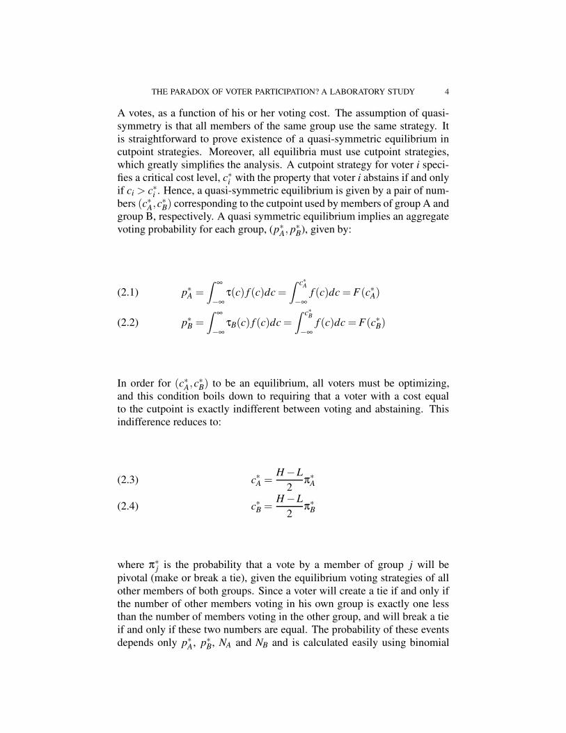
The experiments are based on the Palfrey and Rosenthal (1985) model ofturnout when voters have privately known voting costs. There are N voters,divided into two groups, the supporters of candidate A and the supporters ofcandidate B. In Palfrey and Rosenthal, it was assumed that the two groupswere equal in size, but here we consider the minor extension where the sizeof group A is NA and the size of group B is NB, and NA < NB. The two sizesare assumed to be common knowledge to all voters. We will refer to groupA as the minority group and group B as the majority group. We will refer tocandidate A as the underdog and candidate B as the frontrunner. The votingrule is simple plurality. Voters decide simultaneously whether to cast a votefor their preferred candidate or to abstain. Whichever candidate receivesmore votes wins the election, with ties broken randomly. If candidate Awins then all members of group A receive a reward of H and all members ofgroup B receive a reward of L < H. If candidate B wins then all membersof group B receive a reward of H and all members of group A receive areward of L < H. These reward are common knowledge. Voting is costly,and the voting cost to voter i is denoted ci. Voter i knows ci before decidingwhether to vote or abstain, but the distribution from which the voting costsof other voters are drawn - each voter’s cost is an independent draw fromthe same distribution. The density function of the cost distribution, f (c),exists and is common knowledge and assumed to be positive everywhereon the support.

A quasi-symmetric equilibrium of the voting game is a pair of turnoutstrategies, (τA,τB), where τA specifies the probability a member of group


A votes, as a function of his or her voting cost. The assumption of quasi-symmetry is that all members of the same group use the same strategy. Itis straightforward to prove existence of a quasi-symmetric equilibrium incutpoint strategies. Moreover, all equilibria must use cutpoint strategies,which greatly simplifies the analysis. A cutpoint strategy for voter i speci-fies a critical cost level, c∗i with the property that voter i abstains if and onlyif ci > c∗i . Hence, a quasi-symmetric equilibrium is given by a pair of num-bers (c∗A,c∗B) corresponding to the cutpoint used by members of group A andgroup B, respectively. A quasi symmetric equilibrium implies an aggregatevoting probability for each group, (p∗A, p∗B), given by:

p∗A =Z ∞

−∞τ(c) f (c)dc =

Z c∗A

−∞f (c)dc = F(c∗A)(2.1)

p∗B =Z ∞

−∞τB(c) f (c)dc =

Z c∗B

−∞f (c)dc = F(c∗B)(2.2)

In order for (c∗A,c∗B) to be an equilibrium, all voters must be optimizing,and this condition boils down to requiring that a voter with a cost equalto the cutpoint is exactly indifferent between voting and abstaining. Thisindifference reduces to:

c∗A =H −L

2 π∗A(2.3)

c∗B =H −L

2π∗

B(2.4)

where π∗j is the probability that a vote by a member of group j will be

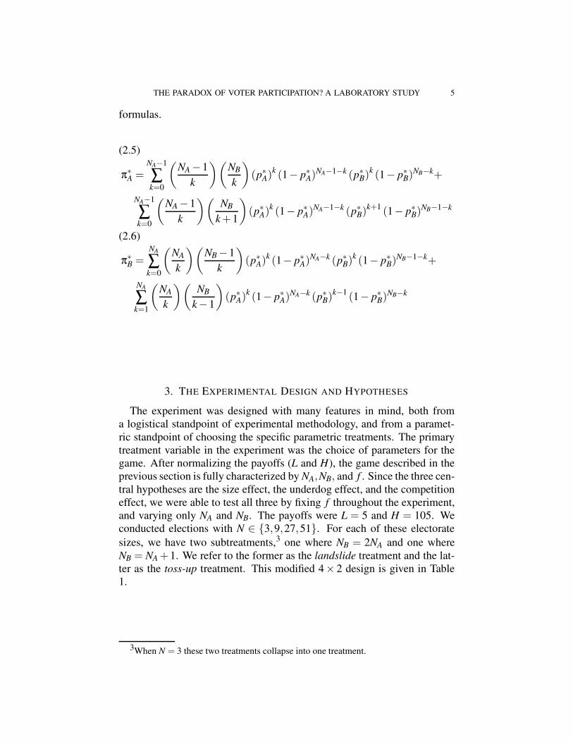
pivotal (make or break a tie), given the equilibrium voting strategies of allother members of both groups. Since a voter will create a tie if and only ifthe number of other members voting in his own group is exactly one lessthan the number of members voting in the other group, and will break a tieif and only if these two numbers are equal. The probability of these eventsdepends only p∗A, p∗B, NA and NB and is calculated easily using binomial


formulas.

π∗A =

NA−1

∑k=0

(NA −1

k

)(NBk

)(p∗A)k (1− p∗A)NA−1−k (p∗B)k (1− p∗B)NB−k+

(2.5)

NA−1

∑k=0

(NA −1

k

)(NB

k +1

)(p∗A)k (1− p∗A)NA−1−k (p∗B)k+1 (1− p∗B)NB−1−k

π∗B =

NA

∑k=0

(NAk

)(NB −1

k

)(p∗A)k (1− p∗A)NA−k (p∗B)k (1− p∗B)NB−1−k+

(2.6)

NA

∑k=1

(NAk

)(NB

k−1

)(p∗A)k (1− p∗A)NA−k (p∗B)k−1 (1− p∗B)NB−k

3. THE EXPERIMENTAL DESIGN AND HYPOTHESES

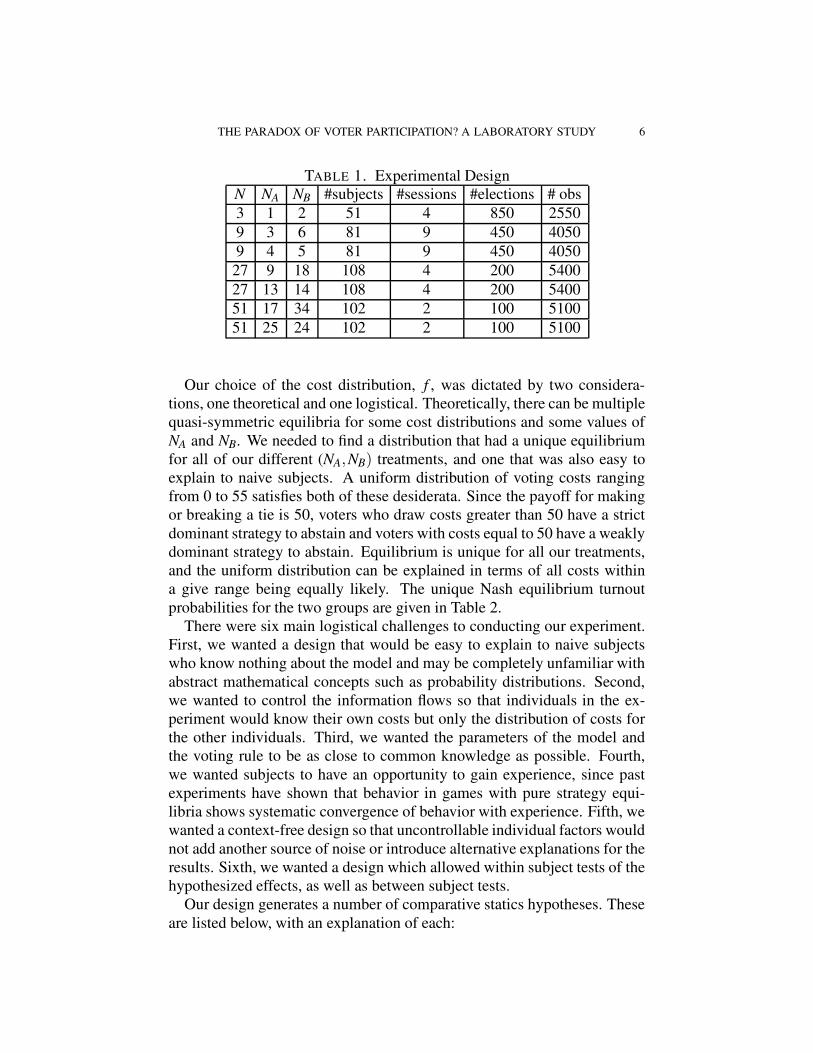
The experiment was designed with many features in mind, both froma logistical standpoint of experimental methodology, and from a paramet-ric standpoint of choosing the specific parametric treatments. The primarytreatment variable in the experiment was the choice of parameters for thegame. After normalizing the payoffs (L and H), the game described in theprevious section is fully characterized by NA,NB, and f . Since the three cen-tral hypotheses are the size effect, the underdog effect, and the competitioneffect, we were able to test all three by fixing f throughout the experiment,and varying only NA and NB. The payoffs were L = 5 and H = 105. Weconducted elections with N ∈ {3,9,27,51}. For each of these electoratesizes, we have two subtreatments,3 one where NB = 2NA and one whereNB = NA +1. We refer to the former as the landslide treatment and the lat-ter as the toss-up treatment. This modified 4× 2 design is given in Table1.

3When N = 3 these two treatments collapse into one treatment.


TABLE 1. Experimental DesignN NA NB #subjects #sessions #elections # obs3 1 2 51 4 850 25509 3 6 81 9 450 40509 4 5 81 9 450 4050

27 9 18 108 4 200 540027 13 14 108 4 200 540051 17 34 102 2 100 510051 25 24 102 2 100 5100

Our choice of the cost distribution, f , was dictated by two considera-tions, one theoretical and one logistical. Theoretically, there can be multiplequasi-symmetric equilibria for some cost distributions and some values ofNA and NB. We needed to find a distribution that had a unique equilibriumfor all of our different (NA,NB) treatments, and one that was also easy toexplain to naive subjects. A uniform distribution of voting costs rangingfrom 0 to 55 satisfies both of these desiderata. Since the payoff for makingor breaking a tie is 50, voters who draw costs greater than 50 have a strictdominant strategy to abstain and voters with costs equal to 50 have a weaklydominant strategy to abstain. Equilibrium is unique for all our treatments,and the uniform distribution can be explained in terms of all costs withina give range being equally likely. The unique Nash equilibrium turnoutprobabilities for the two groups are given in Table 2.

There were six main logistical challenges to conducting our experiment.First, we wanted a design that would be easy to explain to naive subjectswho know nothing about the model and may be completely unfamiliar withabstract mathematical concepts such as probability distributions. Second,we wanted to control the information flows so that individuals in the ex-periment would know their own costs but only the distribution of costs forthe other individuals. Third, we wanted the parameters of the model andthe voting rule to be as close to common knowledge as possible. Fourth,we wanted subjects to have an opportunity to gain experience, since pastexperiments have shown that behavior in games with pure strategy equi-libria shows systematic convergence of behavior with experience. Fifth, wewanted a context-free design so that uncontrollable individual factors wouldnot add another source of noise or introduce alternative explanations for theresults. Sixth, we wanted a design which allowed within subject tests of thehypothesized effects, as well as between subject tests.

Our design generates a number of comparative statics hypotheses. Theseare listed below, with an explanation of each:


Hypotheses

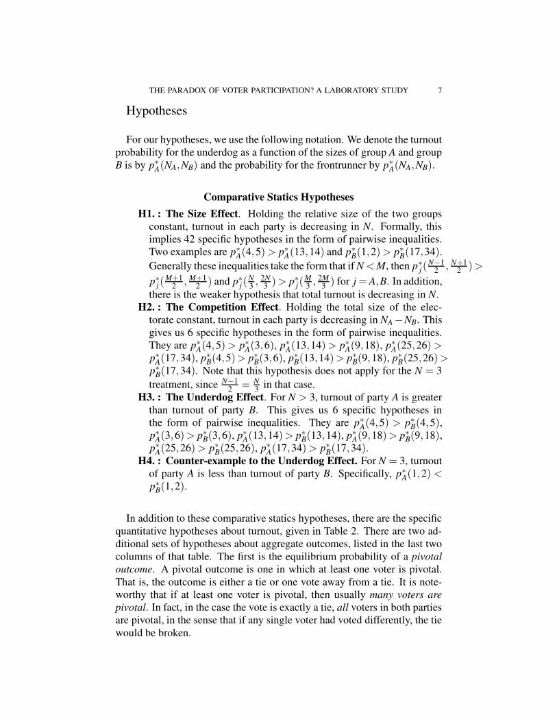
For our hypotheses, we use the following notation. We denote the turnoutprobability for the underdog as a function of the sizes of group A and groupB is by p∗A(NA,NB) and the probability for the frontrunner by p∗A(NA,NB).

Comparative Statics HypothesesH1. : The Size Effect. Holding the relative size of the two groups

constant, turnout in each party is decreasing in N. Formally, thisimplies 42 specific hypotheses in the form of pairwise inequalities.Two examples are p∗A(4,5) > p∗A(13,14) and p∗B(1,2) > p∗B(17,34).Generally these inequalities take the form that if N < M, then p∗j(N−1

2 ,N+1

2 ) >

p∗j(M+12 ,

M+12 ) and p∗j(N

3 ,2N3 ) > p∗j(M

3 ,2M3 ) for j = A,B. In addition,

there is the weaker hypothesis that total turnout is decreasing in N.H2. : The Competition Effect. Holding the total size of the elec-

torate constant, turnout in each party is decreasing in NA−NB. Thisgives us 6 specific hypotheses in the form of pairwise inequalities.They are p∗A(4,5) > p∗A(3,6), p∗A(13,14) > p∗A(9,18), p∗A(25,26) >

p∗A(17,34), p∗B(4,5) > p∗B(3,6), p∗B(13,14) > p∗B(9,18), p∗B(25,26) >

p∗B(17,34). Note that this hypothesis does not apply for the N = 3treatment, since N−1

2 = N3 in that case.

H3. : The Underdog Effect. For N > 3, turnout of party A is greaterthan turnout of party B. This gives us 6 specific hypotheses inthe form of pairwise inequalities. They are p∗A(4,5) > p∗B(4,5),p∗A(3,6) > p∗B(3,6), p∗A(13,14) > p∗B(13,14), p∗A(9,18) > p∗B(9,18),p∗A(25,26) > p∗B(25,26), p∗A(17,34) > p∗B(17,34).

H4. : Counter-example to the Underdog Effect. For N = 3, turnoutof party A is less than turnout of party B. Specifically, p∗A(1,2) <

p∗B(1,2).

In addition to these comparative statics hypotheses, there are the specificquantitative hypotheses about turnout, given in Table 2. There are two ad-ditional sets of hypotheses about aggregate outcomes, listed in the last twocolumns of that table. The first is the equilibrium probability of a pivotaloutcome. A pivotal outcome is one in which at least one voter is pivotal.That is, the outcome is either a tie or one vote away from a tie. It is note-worthy that if at least one voter is pivotal, then usually many voters arepivotal. In fact, in the case the vote is exactly a tie, all voters in both partiesare pivotal, in the sense that if any single voter had voted differently, the tiewould be broken.


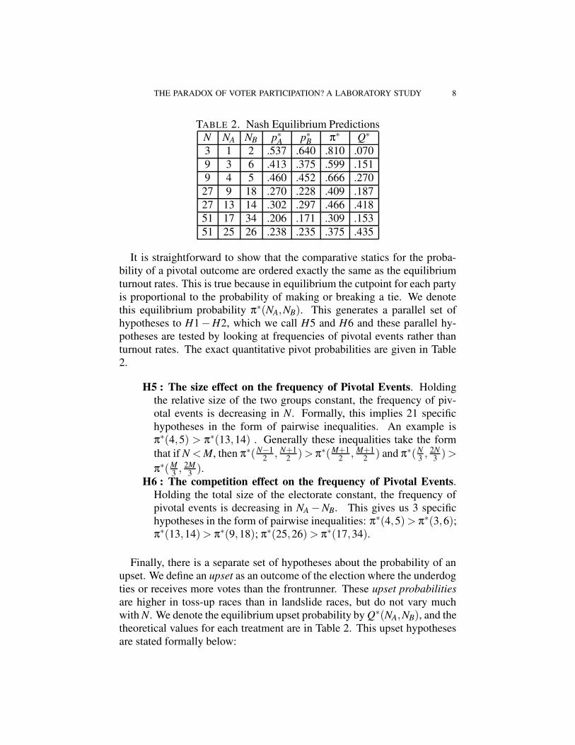
TABLE 2. Nash Equilibrium PredictionsN NA NB p∗A p∗B π∗ Q∗

3 1 2 .537 .640 .810 .0709 3 6 .413 .375 .599 .1519 4 5 .460 .452 .666 .270

27 9 18 .270 .228 .409 .18727 13 14 .302 .297 .466 .41851 17 34 .206 .171 .309 .15351 25 26 .238 .235 .375 .435

It is straightforward to show that the comparative statics for the proba-bility of a pivotal outcome are ordered exactly the same as the equilibriumturnout rates. This is true because in equilibrium the cutpoint for each partyis proportional to the probability of making or breaking a tie. We denotethis equilibrium probability π∗(NA,NB). This generates a parallel set ofhypotheses to H1−H2, which we call H5 and H6 and these parallel hy-potheses are tested by looking at frequencies of pivotal events rather thanturnout rates. The exact quantitative pivot probabilities are given in Table2.

H5 : The size effect on the frequency of Pivotal Events. Holdingthe relative size of the two groups constant, the frequency of piv-otal events is decreasing in N. Formally, this implies 21 specifichypotheses in the form of pairwise inequalities. An example isπ∗(4,5) > π∗(13,14) . Generally these inequalities take the formthat if N < M, then π∗(N−1

2 ,N+1

2 ) > π∗(M+12 ,

M+12 ) and π∗(N

3 ,2N3 ) >

π∗(M3 ,

2M3 ).

H6 : The competition effect on the frequency of Pivotal Events.Holding the total size of the electorate constant, the frequency ofpivotal events is decreasing in NA −NB. This gives us 3 specifichypotheses in the form of pairwise inequalities: π∗(4,5) > π∗(3,6);π∗(13,14) > π∗(9,18); π∗(25,26) > π∗(17,34).

Finally, there is a separate set of hypotheses about the probability of anupset. We define an upset as an outcome of the election where the underdogties or receives more votes than the frontrunner. These upset probabilitiesare higher in toss-up races than in landslide races, but do not vary muchwith N. We denote the equilibrium upset probability by Q∗(NA,NB), and thetheoretical values for each treatment are in Table 2. This upset hypothesesare stated formally below:


H7 : Upset Rates. The underdog is more likely to tie or win in toss-up races than in landslide races, and these upset probabilities aredecreasing in N. This generates 15 specific hypotheses in the formof pairwise inequalities. Twelve of these hypotheses are of the formQ∗(N−1

2 ,N+1

2 ) > Q∗(M+12 ,

M+12 ) and Q∗(N

3 ,2N3 ) > Q∗(M

3 ,2M3 ) for

N < M. The other three hypotheses are Q∗(N−12 ,

N+12 ) > Q∗(N

3 ,2N3 ),

N = 9,27,54.In addition to hypotheses about aggregate behavior, the unique BayesianNash equilibrium also makes very sharp predictions about individual be-havior. Specifically, all individuals should be using exact cutpoint rules.Moreover, these cutpoint rules should be precisely those corresponding tothe turnout rates listed in Table 2. Obviously, hypotheses as sharp as thiswill inevitably be rejected. The cutpoint rules are pure strategies, so a sin-gle violation of the exact cutpoint rule by any subject in will completelyreject the theory. Accordingly, we will pursue these hypotheses in the re-sults section more descriptively, rather than formally testing them. We willhowever, consider a bounded rationality model in which subjects follow acutpoint rule stochastically - that is, they follow it most of the time, but vi-olate it some of the time. This allows us to classify subjects according totheir propensity to vote, which we expect to vary due to many diverse fac-tors such as expectations about pivotal events, risk aversion, attitudes aboutgroup norms, social preferences, judgement fallacies and so forth.

There are also qualitative hypotheses that can be addressed at the indi-vidual level. In our design, subjects were in only one electorate size (3, 9,27, or 51), but participated in a multiple elections, both toss-up and land-slide, and participated as members of both the small group and the largegroup. This is explained in more detail in the next session. Accordingly, weaddress H2, H3, and H4 at the individual level as well as at the aggregatelevel.

4. EXPERIMENTAL PROTOCOL

Subjects were recruited by email announcement from a subject pool con-sisting of registered UCLA students. A total of 284 different subjects par-ticipated in the study. We conduced 20 separate sessions using networkedcomputers at the CASSEL experimental facility.4 In each session, N washeld fixed throughout the entire session. For the N > 3 sessions, there weretwo subsessions of 50 rounds each; one subsession was the toss-up treat-ment and the other subsession was the landslide treatment. The sequencing

4The software was programmed as server/client applications in Java,using the open source experimental software package called Multistage(http://multistage.ssel.caltech.edu/).


of the two treatments was done both ways for each N. Before each round,each subject was assigned to either group A or group B and assigned a vot-ing cost, drawn independently from the uniform distribution between 0 and55, in integer increments.5 Therefore, each subject gained experience as amember of the majority and minority party for exactly one value of N, andparticipated in both 50 landslide and 50 toss-up elections. Instructions wereread aloud so everyone could hear, and Powerpoint slides were projectedin front of the room to help explain the rules and to make all the commonknowledge to the extent possible. After the instructions were read, subjectswere walked through two practice rounds with randomly forced choices andthen were required to correctly answer all the questions on a computerizedcomprehension quiz before the experiment began. After the first 50 rounds,a very short set of new instructions were read aloud, explaining that thesizes of group A and group B would be different for the next 50 rounds.

The wording in the instructions was written so as to induce as neutralan environment as possible.6 There was no mention of voting or winningor losing or costs. The labels were abstract. The smaller groups was re-ferred to the alpha group (A) and the larger group was referred to as thebeta group (B). Individuals were asked in each round to choose X or Y. Ifmore members of A(B) chose X than members of B(A) chose X, then eachmember of A(B) received 105 and each member of group B(A) received 5.In case of a tie, each member of each group received 55 (the expected valueof a fair coin toss). Therefore, voting corresponded to “choosing X” andabstaining corresponded to “choosing Y.” The voting cost was referred toas a “Y bonus,” and was added to a player’s earnings if that player choseY instead of X in an election. Therefore, the voting cost was implementedas an opportunity cost. If a player chose X, that player did not receive theirY bonus for that election. Bonuses were randomly redrawn in every round,independently for each subject, and subjects were only told their own Ybonus. 7

The N = 3 sessions were conducted slightly differently. First, there wereonly 50 rounds, since the toss-up and landslide treatments were identical.Second, the sessions were conducted with either 12 or 15 subjects, whowere randomly rematched each round into subgroups of 3 each period, be-fore being assigned a party and a voting cost. This allowed us to obtain a

5Every 100 points paid off $.37.6A sample of the instructions from one of the 27 person sessions is in the Appendix.7We ran two additional sessions with n = 9 where the instructions were presented in the

context of voting decision in elections, and the two groups were referred to as parties. Theresults were nearly identical and are discussed briefly in the results section.


comparable number of subjects for the N = 3 treatment as the other treat-ments.

5. RESULTS

5.1. Aggregate results. The analysis of results at the aggregate level iscarried out at three levels. First, we look at the empirical turnout rates,and how they vary with respect electorate size, the competitiveness of theelection, and whether voters are from the majority or minority parties. Thisenables us to address hypotheses H1−H4. Next, we focus on outcomes,and show how the empirical frequencies of pivotal events and upsets varywith electorate size and electoral competitiveness.

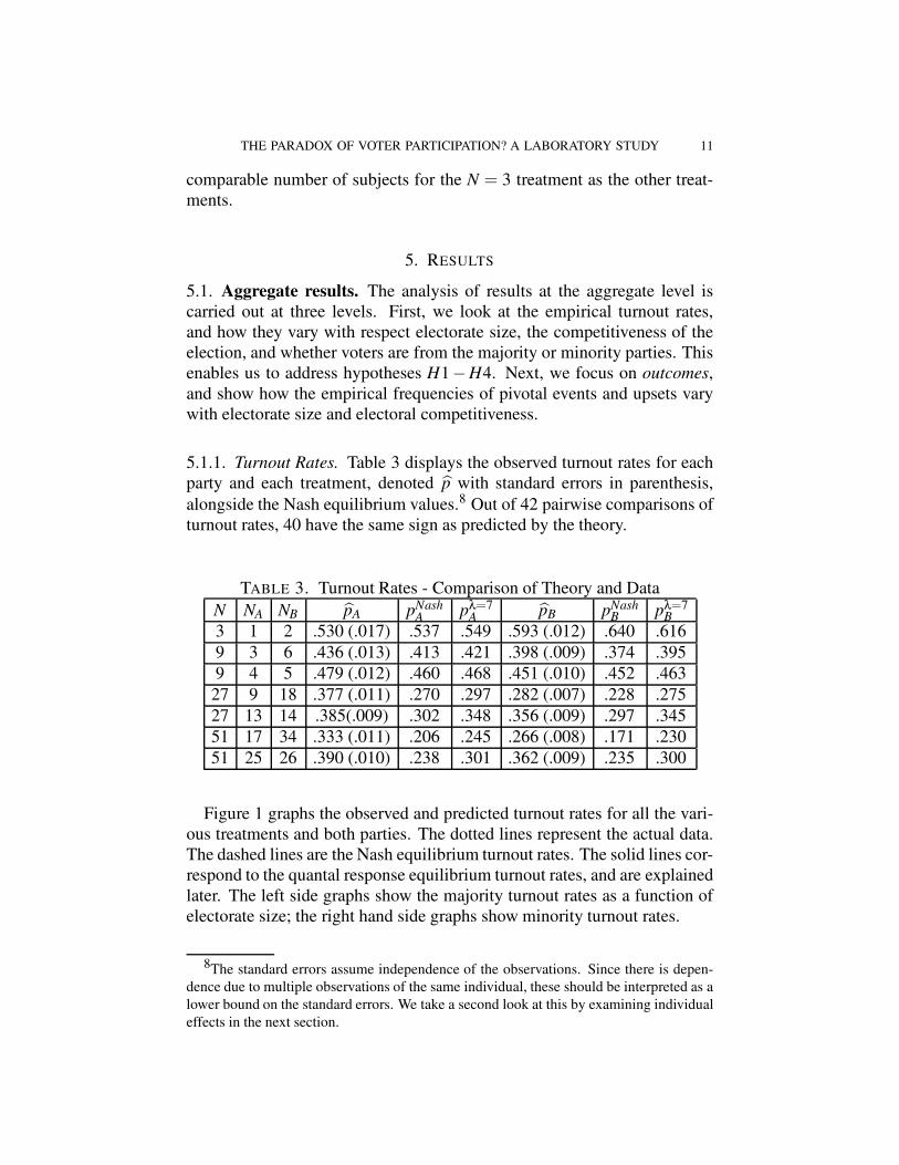
5.1.1. Turnout Rates. Table 3 displays the observed turnout rates for eachparty and each treatment, denoted p with standard errors in parenthesis,alongside the Nash equilibrium values.8 Out of 42 pairwise comparisons ofturnout rates, 40 have the same sign as predicted by the theory.

TABLE 3. Turnout Rates - Comparison of Theory and DataN NA NB pA pNash

A pλ=7A pB pNash

B pλ=7B

3 1 2 .530 (.017) .537 .549 .593 (.012) .640 .6169 3 6 .436 (.013) .413 .421 .398 (.009) .374 .3959 4 5 .479 (.012) .460 .468 .451 (.010) .452 .463

27 9 18 .377 (.011) .270 .297 .282 (.007) .228 .27527 13 14 .385(.009) .302 .348 .356 (.009) .297 .34551 17 34 .333 (.011) .206 .245 .266 (.008) .171 .23051 25 26 .390 (.010) .238 .301 .362 (.009) .235 .300

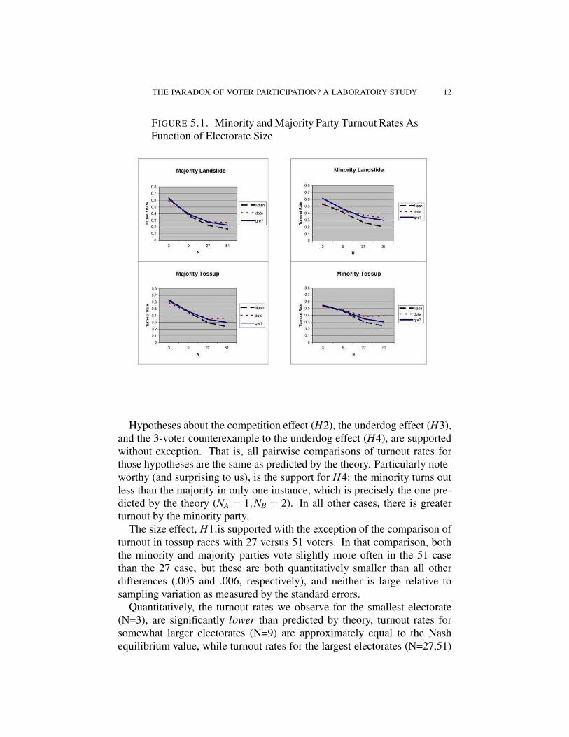
Figure 1 graphs the observed and predicted turnout rates for all the vari-ous treatments and both parties. The dotted lines represent the actual data.The dashed lines are the Nash equilibrium turnout rates. The solid lines cor-respond to the quantal response equilibrium turnout rates, and are explainedlater. The left side graphs show the majority turnout rates as a function ofelectorate size; the right hand side graphs show minority turnout rates.

8The standard errors assume independence of the observations. Since there is depen-dence due to multiple observations of the same individual, these should be interpreted as alower bound on the standard errors. We take a second look at this by examining individualeffects in the next section.


FIGURE 5.1. Minority and Majority Party Turnout Rates AsFunction of Electorate Size

Hypotheses about the competition effect (H2), the underdog effect (H3),and the 3-voter counterexample to the underdog effect (H4), are supportedwithout exception. That is, all pairwise comparisons of turnout rates forthose hypotheses are the same as predicted by the theory. Particularly note-worthy (and surprising to us), is the support for H4: the minority turns outless than the majority in only one instance, which is precisely the one pre-dicted by the theory (NA = 1,NB = 2). In all other cases, there is greaterturnout by the minority party.

The size effect, H1,is supported with the exception of the comparison ofturnout in tossup races with 27 versus 51 voters. In that comparison, boththe minority and majority parties vote slightly more often in the 51 casethan the 27 case, but these are both quantitatively smaller than all otherdifferences (.005 and .006, respectively), and neither is large relative tosampling variation as measured by the standard errors.

Quantitatively, the turnout rates we observe for the smallest electorate(N=3), are significantly lower than predicted by theory, turnout rates forsomewhat larger electorates (N=9) are approximately equal to the Nashequilibrium value, while turnout rates for the largest electorates (N=27,51)


are higher than predicted by theory.9 As a general rule, we find that turnoutrates are closer to .5 than theory predicts. This mirrors findings by Goereeand Holt (2005) for a broad class of games with a similar structure to ourvoter turnout experiments.10

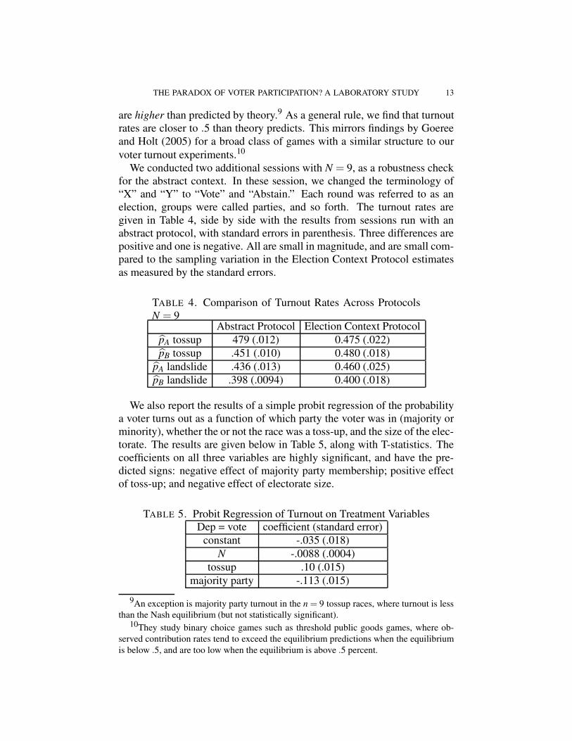
We conducted two additional sessions with N = 9, as a robustness checkfor the abstract context. In these session, we changed the terminology of“X” and “Y” to “Vote” and “Abstain.” Each round was referred to as anelection, groups were called parties, and so forth. The turnout rates aregiven in Table 4, side by side with the results from sessions run with anabstract protocol, with standard errors in parenthesis. Three differences arepositive and one is negative. All are small in magnitude, and are small com-pared to the sampling variation in the Election Context Protocol estimatesas measured by the standard errors.

TABLE 4. Comparison of Turnout Rates Across ProtocolsN = 9

Abstract Protocol Election Context ProtocolpA tossup 479 (.012) 0.475 (.022)pB tossup .451 (.010) 0.480 (.018)

pA landslide .436 (.013) 0.460 (.025)pB landslide .398 (.0094) 0.400 (.018)

We also report the results of a simple probit regression of the probabilitya voter turns out as a function of which party the voter was in (majority orminority), whether the or not the race was a toss-up, and the size of the elec-torate. The results are given below in Table 5, along with T-statistics. Thecoefficients on all three variables are highly significant, and have the pre-dicted signs: negative effect of majority party membership; positive effectof toss-up; and negative effect of electorate size.

TABLE 5. Probit Regression of Turnout on Treatment VariablesDep = vote coefficient (standard error)

constant -.035 (.018)N -.0088 (.0004)

tossup .10 (.015)majority party -.113 (.015)

9An exception is majority party turnout in the n = 9 tossup races, where turnout is lessthan the Nash equilibrium (but not statistically significant).

10They study binary choice games such as threshold public goods games, where ob-served contribution rates tend to exceed the equilibrium predictions when the equilibriumis below .5, and are too low when the equilibrium is above .5 percent.


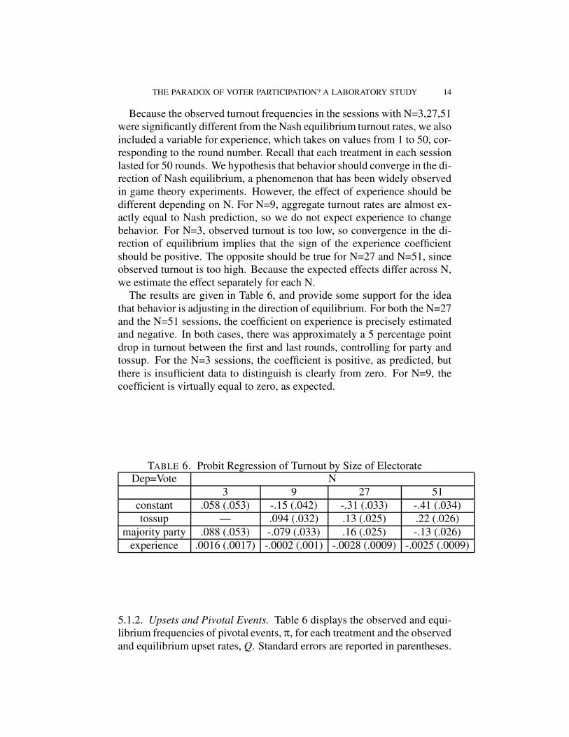
Because the observed turnout frequencies in the sessions with N=3,27,51were significantly different from the Nash equilibrium turnout rates, we alsoincluded a variable for experience, which takes on values from 1 to 50, cor-responding to the round number. Recall that each treatment in each sessionlasted for 50 rounds. We hypothesis that behavior should converge in the di-rection of Nash equilibrium, a phenomenon that has been widely observedin game theory experiments. However, the effect of experience should bedifferent depending on N. For N=9, aggregate turnout rates are almost ex-actly equal to Nash prediction, so we do not expect experience to changebehavior. For N=3, observed turnout is too low, so convergence in the di-rection of equilibrium implies that the sign of the experience coefficientshould be positive. The opposite should be true for N=27 and N=51, sinceobserved turnout is too high. Because the expected effects differ across N,we estimate the effect separately for each N.

The results are given in Table 6, and provide some support for the ideathat behavior is adjusting in the direction of equilibrium. For both the N=27and the N=51 sessions, the coefficient on experience is precisely estimatedand negative. In both cases, there was approximately a 5 percentage pointdrop in turnout between the first and last rounds, controlling for party andtossup. For the N=3 sessions, the coefficient is positive, as predicted, butthere is insufficient data to distinguish is clearly from zero. For N=9, thecoefficient is virtually equal to zero, as expected.

TABLE 6. Probit Regression of Turnout by Size of ElectorateDep=Vote N

3 9 27 51constant .058 (.053) -.15 (.042) -.31 (.033) -.41 (.034)tossup — .094 (.032) .13 (.025) .22 (.026)

majority party .088 (.053) -.079 (.033) .16 (.025) -.13 (.026)experience .0016 (.0017) -.0002 (.001) -.0028 (.0009) -.0025 (.0009)

5.1.2. Upsets and Pivotal Events. Table 6 displays the observed and equi-librium frequencies of pivotal events, π, for each treatment and the observedand equilibrium upset rates, Q. Standard errors are reported in parentheses.


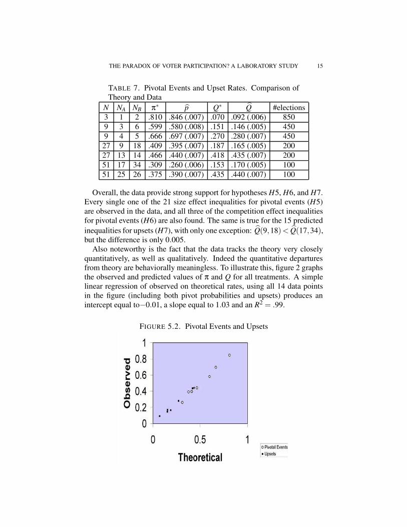
TABLE 7. Pivotal Events and Upset Rates. Comparison ofTheory and Data

N NA NB π∗ p Q∗ Q #elections3 1 2 .810 .846 (.007) .070 .092 (.006) 8509 3 6 .599 .580 (.008) .151 .146 (.005) 4509 4 5 .666 .697 (.007) .270 .280 (.007) 45027 9 18 .409 .395 (.007) .187 .165 (.005) 20027 13 14 .466 .440 (.007) .418 .435 (.007) 20051 17 34 .309 .260 (.006) .153 .170 (.005) 10051 25 26 .375 .390 (.007) .435 .440 (.007) 100

Overall, the data provide strong support for hypotheses H5, H6, and H7.Every single one of the 21 size effect inequalities for pivotal events (H5)are observed in the data, and all three of the competition effect inequalitiesfor pivotal events (H6) are also found. The same is true for the 15 predictedinequalities for upsets (H7), with only one exception: Q(9,18)< Q(17,34),but the difference is only 0.005.

Also noteworthy is the fact that the data tracks the theory very closelyquantitatively, as well as qualitatively. Indeed the quantitative departuresfrom theory are behaviorally meaningless. To illustrate this, figure 2 graphsthe observed and predicted values of π and Q for all treatments. A simplelinear regression of observed on theoretical rates, using all 14 data pointsin the figure (including both pivot probabilities and upsets) produces anintercept equal to−0.01, a slope equal to 1.03 and an R2 = .99.

FIGURE 5.2. Pivotal Events and Upsets


5.2. Quantal Response Equilibrium turnout rates. In this voter partic-ipation game, subjects with cutpoints close to the equilibrium cutpoint arenearly indifferent between voting and abstaining. Consequently, very smallerrors in their judgment about the pivot probabilities, or other factors, couldlead them to make a suboptimal decision. With this in mind, it makes senseto explore models such errors are possible and where the probability of sucherrors are derived endogenously in the model.

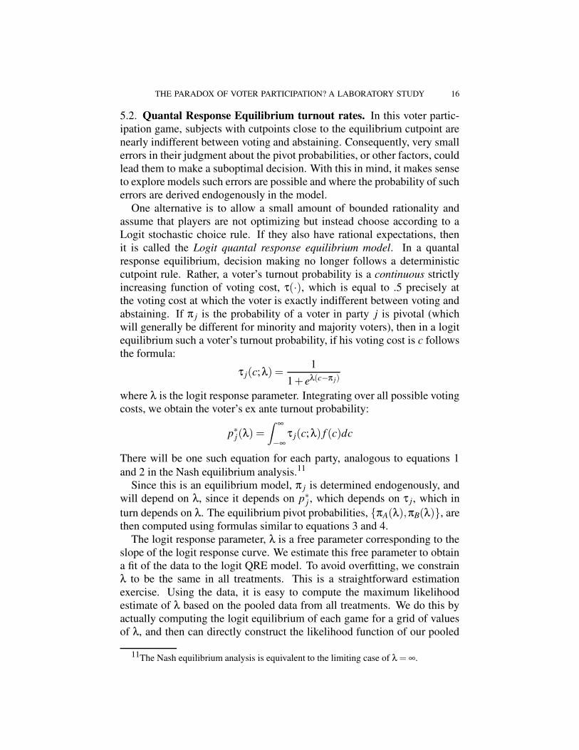
One alternative is to allow a small amount of bounded rationality andassume that players are not optimizing but instead choose according to aLogit stochastic choice rule. If they also have rational expectations, thenit is called the Logit quantal response equilibrium model. In a quantalresponse equilibrium, decision making no longer follows a deterministiccutpoint rule. Rather, a voter’s turnout probability is a continuous strictlyincreasing function of voting cost, τ(·), which is equal to .5 precisely atthe voting cost at which the voter is exactly indifferent between voting andabstaining. If π j is the probability of a voter in party j is pivotal (whichwill generally be different for minority and majority voters), then in a logitequilibrium such a voter’s turnout probability, if his voting cost is c followsthe formula:

τ j(c;λ) =1

1+ eλ(c−π j)

where λ is the logit response parameter. Integrating over all possible votingcosts, we obtain the voter’s ex ante turnout probability:

p∗j(λ) =Z ∞

−∞τ j(c;λ) f (c)dc

There will be one such equation for each party, analogous to equations 1and 2 in the Nash equilibrium analysis.11

Since this is an equilibrium model, π j is determined endogenously, andwill depend on λ, since it depends on p∗j , which depends on τ j, which inturn depends on λ. The equilibrium pivot probabilities, {πA(λ),πB(λ)}, arethen computed using formulas similar to equations 3 and 4.

The logit response parameter, λ is a free parameter corresponding to theslope of the logit response curve. We estimate this free parameter to obtaina fit of the data to the logit QRE model. To avoid overfitting, we constrainλ to be the same in all treatments. This is a straightforward estimationexercise. Using the data, it is easy to compute the maximum likelihoodestimate of λ based on the pooled data from all treatments. We do this byactually computing the logit equilibrium of each game for a grid of valuesof λ, and then can directly construct the likelihood function of our pooled

11The Nash equilibrium analysis is equivalent to the limiting case of λ = ∞.


data, as a function of λ. This yields a maximum likelihood estimate equalto λ = 7.

We then use that estimated value, λ = 7, along with the actual drawsof voting costs, to compute for each treatment and each part, theoreticalQRE turnout rates, denoted pλ=7. These are given in two columns of Table3, and also displayed in Figure 1. Two observations are clear. First, theQRE model fits the data better. Second, the QRE model provides exactlythe right qualitative correction to the Nash model. Recall that the Nashmodel underpredicted turnout in larger elections and overpredicted turnoutin small elections, and did fairly well for intermediate-sized elections. TheQRE predicts less turnout than Nash equilibrium in the smallest election,and more turnout than Nash equilibrium in the large elections. QRE alsopredicts even greater amounts of overvoting (relative to Nash), as the sizeof the election becomes larger and larger, which is what we observed in thedata.

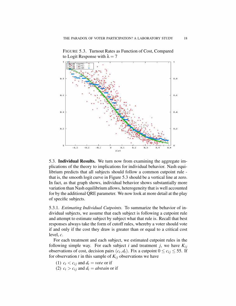
As an alternative way to see how well the logit choice model is capturingvoter behavior, Figure 5.3 graphs turnout rates by “normalized” voting cost.For each treatment and each party, we define a normalized voting cost as thedifference between a voter’s actual voting cost and the logit equilibrium cut-point (for λ = 7). Thus, for example, if the QRE cutpoint for an A voter insome treatment were, say, 15, and their actual cost were 25, their normal-ized voting cost would be 10. Thus our normalization allows us to displayall the voting behavior in a single graph. According to the logit QRE, thevoting probabilities should follow a logit curve, which is the smooth de-creasing curve in the figure (for λ = 7). The decreasing step-function curveaverages the data across normalized cost intervals of .03.


FIGURE 5.3. Turnout Rates as Function of Cost, Comparedto Logit Response with λ = 7

5.3. Individual Results. We turn now from examining the aggregate im-plications of the theory to implications for individual behavior. Nash equi-librium predicts that all subjects should follow a common cutpoint rule -that is, the smooth logit curve in Figure 5.3 should be a vertical line at zero.In fact, as that graph shows, individual behavior shows substantially morevariation than Nash equilibrium allows, heterogeneity that is well accountedfor by the additional QRE parameter. We now look at more detail at the playof specific subjects.

5.3.1. Estimating Individual Cutpoints. To summarize the behavior of in-dividual subjects, we assume that each subject is following a cutpoint ruleand attempt to estimate subject by subject what that rule is. Recall that bestresponses always take the form of cutoff rules, whereby a voter should voteif and only if the cost they draw is greater than or equal to a critical costlevel, c.

For each treatment and each subject, we estimated cutpoint rules in thefollowing simple way. For each subject i and treatment j, we have Ki jobservations of cost, decision pairs (ct ,dt). Fix a cutpoint 0 ≤ ci j ≤ 55. Iffor observation t in this sample of Ki j observations we have

(1) ct < ci j and dt = vote or if(2) ct > ci j and dt = abstain or if


(3) ct = ci j

we say that observation t is consistent with the cutpoint ci j. Otherwise, wesay that observation t is an error with respect to the cutpoint ci j.12 Theestimated cutpoint, ci j is the cutpoint that one that minimizes the number oferrors.13

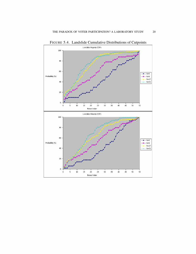
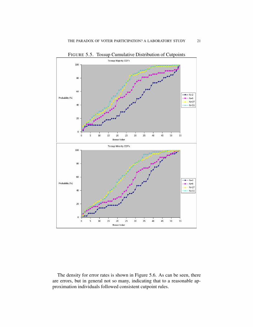
Using this procedure, we can produce a distribution of cutpoints for eachtreatment and a distribution of error rates for each treatment. Figures 5.4and 5.5 show the cumulative distribution of cutpoints for all of the treat-ments.

12Alternatively, one could discount the error by how close the cost is to the cutpoint.This could be done for example by estimating for each i j pair a logit choice function anddefining the estimated cutpoint as the point at which the estimated logit choice probabilityis exactly .5.

13In case there are multiple error-minimizing cutpoints, we use the average of them.


FIGURE 5.4. Landslide Cumulative Distributions of Cutpoints


FIGURE 5.5. Tossup Cumulative Distribution of Cutpoints

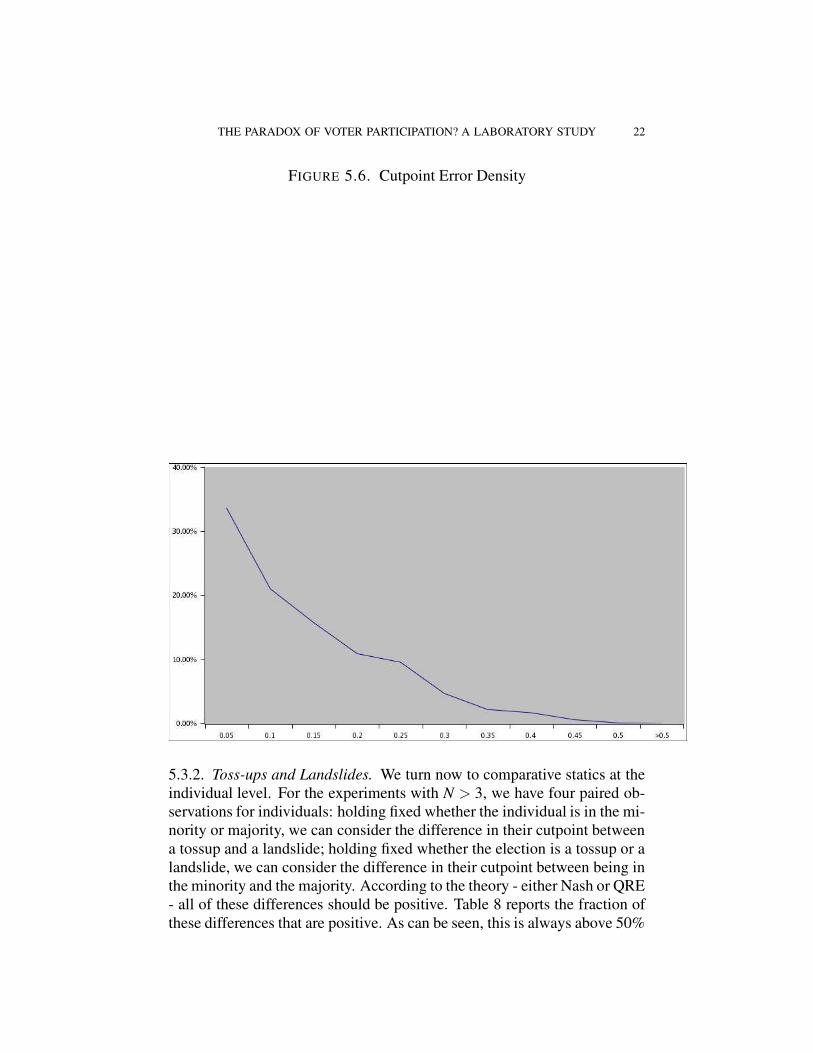
The density for error rates is shown in Figure 5.6. As can be seen, thereare errors, but in general not so many, indicating that to a reasonable ap-proximation individuals followed consistent cutpoint rules.


FIGURE 5.6. Cutpoint Error Density

5.3.2. Toss-ups and Landslides. We turn now to comparative statics at theindividual level. For the experiments with N > 3, we have four paired ob-servations for individuals: holding fixed whether the individual is in the mi-nority or majority, we can consider the difference in their cutpoint betweena tossup and a landslide; holding fixed whether the election is a tossup or alandslide, we can consider the difference in their cutpoint between being inthe minority and the majority. According to the theory - either Nash or QRE- all of these differences should be positive. Table 8 reports the fraction ofthese differences that are positive. As can be seen, this is always above 50%


and generally 60% or higher. This is reinforced by Table 9 which reportsthe average size of these differences. These numbers are all positive.

TABLE 8. Fraction of Positive Paired DifferencesMinority Majority Tossup Landslide

N Tossup-Landslide Tossup-Landslide Minority-Majority Minority-Majority51 0.60 0.75 0.52 0.6527 0.56 0.68 0.56 0.689 0.56 0.60 0.62 0.563 0.57

TABLE 9. Average Size of Paired DifferencesMinority Majority Tossup Landslide

N Tossup-Landslide Tossup-Landslide Minority-Majority Minority-Majority51 3.2 4.4 1.8 3.127 1.1 4.6 1.2 4.79 2.6 1.7 2.7 1.83 0.10

6. CONCLUSIONS

There are six main findings from this voter turnout experiment.First, and most important, all of the comparative statics from the standard

Bayesian Nash equilibrium model of instrumental strategic voting werestrongly supported by the data. We find strong evidence for the size ef-fect, the competition effect, and the underdog effect. The evidence is basedon turnout rates, frequency of pivotal events, and upset probabilities. It isfurther supported by individual level analysis that was possible because ofthe experiment’s mixed within/across subject design, which allows us tocompare an individual subject’s decisions in multiple treatments.

Second, voters are highly responsive to voting cost, with turnout ratesdeclining sharply with the cost of voting. As a first approximation, mostvoters use cutpoint strategies, as predicted by the theory.

Third, a close look at individual behavior reveals that few voters use exactdeterministic cutpoint strategies; choice behavior appears to have a stochas-tic element. This replicates a finding from several other studies of gameswith binary choices and continuous types, where best response rules arecutpoint strategies.14

14See, for example, Casella, Gelman, and Palfrey (2005), Palfrey and Prisbrey (1997),and Palfrey and Rosenthal (1991).


Fourth, voters were less responsive to changes in the parameters of theenvironment than the equilibrium. In particular, this resulted in turnout ratesthat were too low for N = 3 and that exceeded the Nash equilibrium ratesfor the larger groups, with overvoting especially noticeable in the N = 51treatment.

Fifth, an equilibrium approach based on the logit version of QRE, whichincorporates the kind of stochastic choice observed at the individual level,provides a significant improvement in fit over the Nash model, as well asproviding an explanation for undervoting (relative to Nash) in small elec-tions and overvoting in large elections. Furthermore, the responsiveness ofparticipation rates to voting costs is tracked very closely by a logit curve(Figure 3). Nonetheless, the logit QRE model may not fully account for themagnitude of overvoting in the largest elections of our sample, unless thereare higher error rates (smaller λ) in larger elections, a possibility which doesnot have an obvious rationale a priori.

Sixth, the experiment was conducted in a neutral abstract context with nomention of voting, or winning, or parties or elections. In the two extra ses-sions conducted specifically in a voting context, subject behavior was thesame as the abstract context. Hence the phenomena we observe apparentlyare not limited to elections, but are more general. In particular the observa-tion of overvoting relative to the equilibrium cannot be easily dismissed byappealing to arguments such as citizen duty, high school civics classes, orfear that one’s spouse of workmates will castigate one for not voting.

The challenge now is to come up with an explanation of over voting thatis not specific to elections, but applies more broadly to participation gamesin general. The one alternative explored here, QRE, provides a partial ex-planation, but undershoots the overvoting in large elections. Another ex-planation we have considered, that voters systematically overestimate theprobability of being pivotal, is directly contradicted by the N = 3 data,where we observe overvoting. For the same reason, our data also contradictsgroup-specific altruism models, and also the group-utilitarian approach ofHarsanyi (1980), recently proposed as an explanation of high voter turnoutby Feddersen and Sandroni (2002).

Another alternative model minimax regret, is due to Ferejohn and Fio-rina. That model is easily rejected, because it implies that turnout shouldindependent the probability of being decisive, which contradicts the sizeeffect, the competition effect, and the underdog effect.

We conjecture that some kind of mixture of models such as these, thatwould include a variety of behavioral types, will ultimately be needed fora more complete explanation of this phenomenon. One framework forbuilding and estimating such models has been developed by El-Gamal and


Grether (1995), and such an approach may be worth exploring here. How-ever, developing a specification of types for the voting context that is notsimply ad hoc would be a challenge, and the actual computation and esti-mation of such a model may be difficult.

In conclusion, the strength of the comparative statics results should notbe understated. The fact that the experiment clearly supports the three mainequilibrium comparative static effects (size, competition, and underdog) inparticipation games, and the finding that voters use approximate cutpointstrategies, demonstrates that voting behavior is highly strategic, with votersresponding to both the cost of voting and the probability of being pivotal.


REFERENCES

[1] Casella, A., A. Gelman, and T. Palfrey. 2005. “An Experimental Study of StorableVotes.” Games and Economic Behavior. Forthcoming.

[2] Cason, T. and V.-L. Mui, 2005. “Uncertainty and resistance to reform in laboratoryparticipation games. “European Journal of Political Economy. forthcoming

[3] Coate, Stephen and M. Conlin. 2005. “A Group Rule-Utilitarian Approach to VoterTurnout: Theory and Evidence.” American Economic Review. Forthcoming.

[4] Downs, A. 1957. An Economic Theory of Democracy. New York: Harper and Row.[5] El-Gamal, M. and D. Grether. “Are People Bayesian? Uncovering Behavioral Strate-

gies.” Journal of the American Statistical Association. 90, 1137-45.[6] Grosser, Jens, T. Kugler, and A. Schram. 2004. “Preference Uncertainty and Voter

Participation: An Experimental Study.” Working Paper. University of Amsterdam.[7] Feddersen, T. and A. Sandroni (2002), “A Theory of Participation in Elections with

Ethical Voters.” Working Paper. Northwestern University.[8] Goeree, J, and C. Holt. 2005. “An Explanation of Anomalous Behavior in Models of

Political Participation” American Political Science Review.[9] Green, D. and I. Shapiro. 1994. Pathologies of Rational Choice Theory. New Haven:

Yale University Press.[10] Grofman, B. 1993. “Is Turnout the Paradox that Ate Rational Choice Theory?” in In-

formation, Participation, and Choice. ed. B. Grofman. University of Michigan Press:Ann Arbor.

[11] Grosser, J., T. Kugler and A. Schram. 2005. “Preference Uncertainty, Voter Partici-pation and Electoral Efficiency: An Experimental Study.” mimeo Cologne.

[12] Hansen, S., T. Palfrey, and H. Rosenthal. 1987. “The Downsian Model of ElectoralParticipation: Formal Theory and Empirical Analysis of the Constituency Size Ef-fect.” Public Choice. 52: 15-33.

[13] Harsanyi, J. (1980). “Rule Utilitarianism, Rights, Obligations, and the Theory ofRational Behavior.” Theory and Decision. 12: 115-33.

[14] Palfrey, T. and J. Prisbrey. 1997. “Anomalous Behavior in Linear Public Goods Ex-periments: How Much and Why?” American Economic Review. 87, 829-46.

[15] Palfrey, T. and H. Rosenthal. 1983. “A Strategic Calculus of Voting.” Public Choice.[16] Palfrey, T. and H. Rosenthal. 1985. “Voter Participation and Strategic Uncertainty.”

American Political Science Review. 79: 62-78.[17] Palfrey, T. and H. Rosenthal. 1991. “Testing Game-Theoretic Models of Free Riding:

New Evidence on Probability Bias and Learning,” in Laboratory Research in PoliticalEconomy (T. Palfrey, ed.), University of Michigan Press:Ann Arbor.

[18] Schram, A. and J. Sonnemans (1991), “Why people vote: Free riding and the pro-duction and consumption of social pressure,” Journal of Economic Psychology 12,575-620.

[19] Schram, A. and J. Sonnemans (1996), “Why people vote: Experimental evidence,”Journal of Economic Psychology 17, 417-442.

[20] Schram, A. and J. Sonnemans (1996), “Voter Turnout as a Participation Game: AnExperimental Investigation,” International Journal of Game Theory 25, 385-406.


APPENDIXSample instructions from a 9 person session (abstract protocol)

Thank you for agreeing to participate in this research experiment ongroup decision making. During the experiment we require your complete,undistracted attention. So we ask that you follow instructions carefully.Please do not open other applications on your computer, chat with otherstudents, read books or do homework.

For your participation, you will be paid in cash, at the end of the experi-ment. Different participants may earn different amounts. What you earn de-pends partly on your decisions, partly on the decisions of others, and partlyon chance. So it is important that you listen carefully, and fully understandthe instructions before we begin. There will be a short comprehension quizafter the upcoming practice round, which you all need to pass before wecan begin the paid sessions.

The entire experiment will take place through computer terminals, andall interaction between you will take place through the computers. It isimportant that you not talk or in any way try to communicate with otherparticipants during the experiments, except according to the rules describedin the instructions.

We will start with a brief instruction period. During the instruction pe-riod, you will be given a complete description of the experiment and willbe shown how to use the computers. If you have any questions during theinstruction period, raise your hand and your question will be answered outloud so everyone can hear. If any difficulties arise after the experiment hasbegun, raise your hand, and an experimenter will come and assist you pri-vately.

Please open your envelope and remove the Record Sheet. Do not losethis Record Sheet, as you will need the sheet throughout the experiment torecord your earnings.

This experiment will begin with two brief practice sessions to help fa-miliarize you with the rules. The practice session will be followed by 2different paid sessions. Each paid session will consist of 50 rounds.

At the end of the last paid session, you will be paid the sum of what youhave earned in the two paid sessions, plus the show-up fee of $5.00. Ev-eryone will be paid in private and you are under no obligation to tell othershow much you earned. Your earnings during the experiment are denomi-nated in POINTS. Your DOLLAR earnings are determined by multiplying


your earnings in POINTS by a conversion rate. In this experiment, the con-version rate is 0.0037, meaning that 100 POINTS is worth 37 cents.

There are 9 participants in today’s experiment. You will participate in 2brief practice sessions and then 2 paid sessions of 50 rounds each.

Please turn your attention to the screen at the front of the room. We willdemonstrate how the rounds are played.

SCREEN 1 (menu)Everyone should have a screen like the screen projected on stage. If you

have something different from what is projected on stage, please raise yourhand and the staff will assist you.

[CHECK TO SEE IF ANYONE RAISES THEIR HAND]Please do not begin unless we tell you to do so. Please have your attention

focused on the stage during this demonstration period. Please click on theMENU icon. This will bring up screen 2 showing the icons underneath.

SCREEN 2 (icons)On this second screen click on the MULTISTAGE CLIENT icon. A pop

up window will appear right in front of you.SCREEN 3 (client information)Enter your first and last name in the box that appears and then click sub-

mit. You will then see screen 4SCREEN 4 (initializing)Once everyone has logged in, you will be randomly assigned to one of

two groups the ALPHA group or the BETA group. You will see screen 5SCREEN 5 (user interface)At the top of the screen is your id number. Please record this on your

Record Sheet. Below this the screen informs you which group you are inand how many members there are in each group. In this practice session,the ALPHA group has 4 members and the BETA group has 5 members.Next on the screen is a table, describing how your earnings depend on yourchoice of either X or Y and on which group has the most members choosingX. The display in front of the room shows you what the screen looks likefor a member of the Alpha group. It also tells you what your Y bonus is.We will explain what this means in a moment.

You will choose either X and Y by highlighting the corresponding rowlabel and clicking with your mouse.

SCREEN 6x and 6y and 7 (showing highlighting)Your earnings are computed in the following way. It is very important

that you understand this, so please listen carefully. Suppose you chooseX. If your group has more members choosing X than the other group, thenyou will earn 105 points; if both groups have the same number of memberschoosing X, then you will earn 55 points, and if the other group has moremembers choosing X than your group, then you will earn 5 points.


Alternatively, suppose you choose Y. If your group has more memberschoosing X than the other group, then you will earn 105 points plus yourY bonus; if both groups have the same number of members choosing X,then you will earn 55 points plus your Y bonus, and if the other group hasmore members choosing X than your group, then you will earn 5 pointsplus your Y bonus. The amount of your Y-bonus is assigned randomly bythe computer and is shown in the fourth line down from the top of yourscreen. In any given round you have an equal chance of being assignedany Y-bonus between 0 and 55 points. Your Y-bonus in each round doesnot depend on your Y-bonus or decisions in previous rounds, or on the Y-bonuses and decisions of other participants. Since Y-bonuses are assignedseparately for each participant, different participants will typically have dif-ferent Y-bonuses. While you are told your own Y-bonus, you are never toldthe Y-bonuses of other participants. You only know that each of the otherparticipants has a Y-bonus that is some number between 0 and 55.

Here is an example: Suppose that one member of the ALPHA groupchose X and two members of the BETA group choose X. Then the BETAgroup has more members choosing X than the ALPHA group. Each mem-ber of the ALPHA group who chose X earns 5 points; each member of theALPHA group who chose Yearns 5 points plus his or her own personal Y-bonus ; the members of the BETA group who chose X earn 105 points, andeach member of the BETA group who chose Yearns 105 points plus his orher personal Y-bonus.

The bottom of the screen contains a history panel. During the varioussessions and rounds, this panel will be updated to reflect the history of yourpast sessions.

After you and the other participants have all made your choices of Xor Y the screen will change to highlight the row corresponding to your ownchoice, and the column of the group which had the greatest number of mem-bers choose X.

At the end of each round until the session ends, you will be randomlydivided between groups, and will have the opportunity to choose between Xand Y. In other words, you will not necessarily be in the same group duringeach round. At the end of each session, you will see a screen summarizingthe amount that you earned.

SCREEN 8 (match complete)If you have any questions at this time, please raise your hand and

ask your question so that everyone in the room may hear it.PRACTICE SESSION[BRING UP PAYMENT SCREEN FOR PRACTICE SESSION]We will now give you a chance to get used to the computers with a short

practice session. Please take your time, and do not press any keys or use


your mouse until instructed to do so. You will NOT be paid for this ses-sion, it is just to allow you to get familiar with the experiment and yourcomputers.

If your ID number is even, please highlight the Y row and click; if yourID number is odd, please highlight the X row and click. Once everyone hasmade their selection, the results from this first practice round are displayedon your screen.

Remember, you are not paid for this practice round.We will now proceed to the second practice round. Notice that you may

have been reassigned to a new group, since the group assignments are shuf-fled randomly between each round. Please make the opposite choice fromthe choice you made in the first practice round. That is, if your ID numberis even, please highlight the X row label and click; if your ID number isodd, please highlight the Y row label and click. Once everyone has madetheir selection, the results from this second practice round are displayed onyour screen.

Since this is the end of the practice round, your total earnings for thispractice session are displayed on your screen in points (though of course,you wont actually receive that money). We have now completed the practicesession.

[QUIZ]You will notice that a quiz has popped up on your screen. Please read

each question carefully and check the correct answer. Once everyone hasanswered the questions correctly, you may all go on to the second stage ofthe quiz. After successfully completing the second round of questions, wewill commence with the first paid session. If you have difficulty with thequiz or have other questions please your hand.

[END QUIZ]The first paid session will follow the same rules as the practice session.

Let me summarize those rules before we start. Please listen carefully. Ineach round of this session, 4 players will be randomly assigned to the AlphaGroup and 5 players will be assigned to the Beta Group. You may chooseX or Y. As you can see on the table of this screen, if you choose X, yourpayoff will be 105 POINTS if your group has more members choosing Xthan the other group, 5 POINTS if your group has fewer members choosingX, and 55 POINTS if it is a tie. If you choose Y, you will also receive theY-bonus shown on your screen..

There will be 50 rounds in this session. After each round, group assign-ments will be randomly reshuffled. Therefore, in some rounds you will bein the Alpha group and in other rounds you will be in the Beta group. Ineither case, everyone is told which group they are in before making a choiceof X or Y.


Are there any questions before we begin the first paid session[Answer questions.]Please pull out your dividers.SESSION 1We will now begin with session 1. Do not click anything else on the

screen until you are told to do so.[BRING UP PAYMENT SCREEN FOR SESSION 1]Please begin.(Play rounds 1 50)Session 1 is now over. Please record your total payoffs for this session

on your record sheet.[WAIT FOR STAFF TO VERIFY PARTICIPANTS RECORD SHEET]SESSION 2We will now begin session 2.[BRING UP PAYMENT SCREEN FOR SESSION 2]The second paid session will be slightly different from the first session.

Let me summarize those rules before we start. Please listen carefully. Ineach round of this session, 3 players will be randomly assigned to the AlphaGroup and 6 players will be assigned to the Beta Group. You may chooseX or Y. As you can see on the table of this screen, if you choose X, yourpayoff will be 105 POINTS if your group has more members choosing Xthan the other group, 5 POINTS if your group has fewer members choosingX, and 55 POINTS if it is a tie. If you choose Y you will also receive theY-bonus shown on your screen..

There will be 50 rounds in this session. After each round, group assign-ments will be randomly reshuffled. Therefore, some rounds you will be inthe Alpha group and other rounds you will be in the Beta group. In eithercase, everyone is told which group they are in before making a choice of Xor Y.

Are there any questions before we begin the second paid session?Please Begin.(Play rounds 1-50)Session 2 is now over. Please record your total payoffs for this session

on your record sheet.

the paradox of voter participation? a ...lyariv/political_economy_files/...the paradox of voter...

Documents