The Paradox of Skill: Lessons from Golf

1

Richard J. Rendleman, Jr.

April 6, 2015

1Richard J. Rendleman, Jr. is Visiting Professor, Tuck School of Business at Dartmouth and ProfessorEmeritus, Kenan-Flagler Business School, University of North Carolina, Chapel Hill. The author thanks thePGA TOUR for providing the ShotLink data used in connection with this study and Ken Lovell, Je↵ Adams,and Royce Thompson, all associated with the PGA Tour, for providing useful background information. He isespecially thankful to Philip Howard, who provided invaluable assistance with respect to the mathematicalderivations shown in the appendix and to Mark Broadie, who provided comments in the early stages ofthis work. The author also thanks Jon Lewellen and Kent Womack for helpful comments. Please addresscomments to Richard J. Rendleman, Jr. (e-mail: richard rendleman@unc.edu; phone: (919) 962-3188).

1. Introduction

“As skill improves, performance becomes more consistent, and therefore, luck becomes more im-

portant” (Mauboussin 2012, p. 53). This is “the paradox of skill,” based on insights of Gould

(2003) and ‘coined’ and developed further by Mauboussin (2012). Framing the paradox of skill in

terms of the evolution of skill and luck over time, Mauboussin shows that between 1932 and 2008,

the winning time in the men’s Olympic marathon dropped by twenty-five minutes. At the same

time, the gap between the winning time and that of the 20th-place finisher fell from forty to nine

minutes. Similarly, in explaining why no Major League Baseball player since Ted Williams has

recorded a batting average1 of .400 or better, Gould shows that since Williams’ time (Williams’

batting average was .406 in 1941), the skill of batters, pitchers and fielders in general has improved,

while the variance in performance has narrowed. As a result, it has been very di�cult for players in

the modern era to match Williams’ batting average. According to Mauboussin (p. 58) “If everyone

gets better at something, luck plays a more important role in determining who wins.”

The paradox of skill can also be framed in cross-sectional terms. Presumably, for a given activity,

the variance of skills for high-skill populations will be lower than that of lower-skill populations

involving the same activity.2 For example, one would reasonably expect that the variance of skills

among college baseball players would be substantially higher than that of Major League players

and that within the college baseball ranks, the variance should increase in going from Division I

(the highest level of competition) to Division III (the lowest level). As a result, it should be much

easier for a college player to bat .400 compared with a player in the major leagues, and it should

also be easier for college players at the Division II and III levels to bat .400 or better compared with

Division I players. In fact, during the 2013-2014 college baseball season, seven Division I players,

32 Division II players, and 100 Division III players recorded batting averages of .400 or better.3 At

the same time, the highest batting average in the Major Leagues was that of Jose Altuve, who hit

1In baseball, a player’s batting average is the number of hits recorded by the player divided by his “at bats.” “Atbats” is the number of times the player completes his opportunity to hit, less the number of times he reaches firstbase in a fashion that does not involve a hit, such as a walk (“base on balls”) and the number of sacrifice hits. Bytradition, batting averages are expressed without a zero preceding the decimal and expressed verbally as if they hadbeen multiplied by 1,000.

2See Mauboussin (2012, pp. 82-84) for a discussion of how skill will improve, while variation in skill shrinks, asthe population of individuals engaged in a given activity grows.

3Source: http://web1.ncaa.org/stats/StatsSrv/rankings, last accessed on March 25, 2015.

1

0.341.4

The cross-sectional version of the paradox of skill appears to be confirmed in studies by Levitt,

Miles, and Rosenfield (2012) and Levitt and Miles (2014) in response to the 2006 passage of the

Unlawful Internet Gambling Enforcement Act. These two groups studied the extent to which skill

and luck contribute to determining who wins and loses in the popular game of Texas Hold ‘Em

poker. By studying outcomes in the 2010 World Series of Poker (a series of 57 separate tournaments

conducted between May 28 and July 17 at the Rio All Suite Hotel and Casino in Paradise, Nevada),

which, arguably, attracts the the best among professional poker players, Levitt and Miles (2014)

found that players identified from rankings as the most highly skilled at the beginning of Series were

far more successful than players who were not so identified. Levitt, Miles, and Rosenfield (2012)

studied outcomes between May 2006 and May 2007 on an online poker site, which, presumably,

attracts players of lower skill on average compared with World Series participants. They find that

expected payo↵s vary widely across players and “resoundingly” reject the hypothesis that no-limit

Texas Hold ‘Em is a game of pure luck.

Croson, Fishman, and Pope (2008) also study the skill versus luck question in connection with

the World Series of Poker. They find that there is a significant skill component in determining

relative success among the top 18 finishers in 2001-2005 World Series events and that the skill/luck

mix is comparable to that of players who finish among the top-18 in professional golf tournaments

conducted by the PGA Tour. Although they find “the skill di↵erences among top poker players

are similar to skill di↵erences across top golfers” (p. 28), earlier they state “if the [regression]

coe�cients in golf are not statistically di↵erent than those in poker, we will conclude that poker

has similar amounts of skill (and luck) as golf” (p. 27).

The cross-sectional version of the paradox of skill and the results I present in this paper suggest

that a conclusion that “poker has similar amounts of skill (and luck) as golf” may not be warranted

in a study that focuses only on the most highly skilled. As I will show in this paper, the skill/luck

mix varies widely in golf. At the PGA Tour level, the highest level of competition in professional

4Source: http://espn.go.com/mlb/statistics, last accessed March 25, 2015. It should also be noted that aluminumbats are used in college, which, apparently, lead to more hits than wooden bats, which are used in the major leagues.Di↵erence in bat composition could explain some of the gap between Major League batting averages and those atthe Division I college level but, certainly, not the entire gap.

2

golf, players are very homogeneous in skill, and therefore, luck plays a large role in determining

player success in any given event. On the other hand, in amateur competition involving players of

much lower skill, skill can play a larger role than luck in determining tournament outcomes. Thus,

a conclusion that one activity involves a comparable mix of skill and luck as another, when only

the most highly skilled are studied, can be misleading, especially if it takes great skill to reach the

highest level and player skills at the highest level are very homogeneous.5

1.1. Skill versus Luck in Non-Sports-Related Activities

Characterizing a performance activity in terms of its skill and luck components is of interest not

only in sports and games but in many other areas including business, investing, and life in general.

When the question of skill versus luck has been studied in business and investing, the focus has

tended to be on business and investment populations for which data is readily available. Since far

more data has been available for large businesses and large portfolio investors, when the question

of skill versus luck has been studied, the data itself has tilted the skill versus luck question to-

ward (presumably) the most highly skilled. Only recently have the the performance attributes of

lower-skilled populations been studied.6 An excellent example is the study of performance and be-

havioral tendencies among individual investors championed by Barber and Odean and summarized

in Barber and Odean (2013). Although researchers other than Barber and Odean have studied

the investment performance of individual investors, the data used in these studies have been either

proprietary or di�cult to acquire.7,8 Otherwise, the question of skill versus luck in investing has

focused almost entirely on mutual fund performance9 and the performance of institutional investors

5While it is the case that the World Series of Poker attracts poker’s finest players, World Series events are opento anyone willing to pay the entry fee, which can vary from $1,000 to $50,000 per event. As a result, if skill plays arole in determining success and failure in poker, it should be revealed in a study of World Series events.

6A notable exception is the work on individual investor performance initiated by Lease, Lewellen, and Schlarbaum(1974) and continued by the same authors in related studies through 1978.

7Rather than make specific reference to the other researchers, I simply refer the reader to Barber and Odean’sexcellent review paper (2013), which lists and summarizes the most influential and relevant studies in this area.

8In email correspondence, Odean has indicated that he has made his U.S. data available to over 100 academicresearchers, but that U.S. data sets used by other researchers are few and di�cult to obtain. Similarly, he indicatesthat individual investor data for China, India, Germany, Netherlands, and Australia used in other studies is notgenerally available. On the other hand, researchers can gain access to data for Sweden, Norway, and Finland throughgovernment agencies. Even though Odean has made his data available to many researchers, it is not updated regularly,as would be the case with most commercially-available data sets.

9Excellent examples include Grinblatt and Titman (1989), Grinblatt and Titman (1992), Carhart (1997), Daniel,Grinblatt, Titman, and Wermers (1997), Chevalier and Ellison (1999), Kosowski, Timmermann, Wermers, and White

3

in general (Lewellen 2011). Although most mutual fund and institutional investor studies di↵er in

methodology, focus, and the period of time studied, in the broadest of terms, the evidence shows

that if this set of investors can beat the market on a risk- and fee-adjusted basis, it is not by much.

By contrast, the overwhelming evidence is that the performance of individual investors in the long

run is far worse. A similar line of research examines the performance of venture capital and pri-

vate equity funds (for example, Kaplan and Schoar (2005), Phalippou and Gottschalg (2009), and

Phalippou (2010)).

In the more general business realm, a number of studies have addressed the question of “pay-for-

luck” in CEO compensation, including Bertrand and Mullainathan (2001), Garvey and Milbourn

(2006), Bebchuck, Grinstein and Peyer (2010), Cremers and Grinstein (2014), and Bennett, Custdio

and Cvijanovi (2014), among others. In each of these studies, the focus is on CEO performance in

relatively large corporations.10 By contrast, there has been almost no work on the role of luck in

the compensation of small business executives.

In other areas of business, Near and Olshavsky (1985) o↵er an analysis of whether the success

of Japanese automakers has been due to skill or luck. Henderson, Raynor, and Ahmed (2012) study

the extent to which a firm must perform at a high level to eliminate randomness as a su�cient

explanation for its success. Gompers, Kovner, Lerner, and Scharfstein (2010) study the role of skill

among venture-capital-backed entrepreneurs and find that entrepreneurs who are successful in an

initial venture are more likely to be successful in a second compared with those starting a venture

(2006), Cremers and Petajisto (2009), Barras, Scaillet, and Wermers (2010), Fama and French (2010), Berk and vanBinsbergen (2013), Hunter, Kandel, Kandel, and Wermers (2014), and del Guercio and Reuter (2014).

10Bertrand and Mullainathan (p. 902) find that “CEO pay is as sensitive to a lucky dollar as to a general dollar,”but that pay for luck is strongest among poorly-governed firms. Their finding that CEO pays is equally sensitiveto lucky and general dollars is confirmed by Garvey and Milbourn (2006), but they also show that executive pay isinsulated from bad luck. Cremers and Grinstein (2014) also show that CEOs are paid for luck outcomes, but thatthe e↵ect is greater in industries with a high percentage of outsider CEOs. Bennett, Custdio and Cvijanovi (2014)find that CEOs are rewarded for their reactions to luck rather than to pure luck itself. Bebchuck, Grinstein andPeyer (2010) show that CEOs benefit from the opportunistic timing of “lucky” stock option grants given on days ofthe month with the lowest stock price and that the benefit is the greatest when board members are compensated insimilar fashion.

Bertrand and Mullainathan study the pay and performance for 51 of the largest American oil companies for years1977-1994. They also employ a data set of 792 large corporations provided by Yermack (1995) covering the 1984-1991 period. “To be included, firms must qualify for Forbes magazines annual list of the 500 largest U.S. publiccorporations in any of the categories of sales, assets, net income, or market capitalization at least four times between1984 and 1991” (Yermack 1995, p. 248). The studies of Garvey and Milbourn, Cremers and Grinstein, and Bennett,Custdio and Cvijanovi employ ExecuComp data, which covers companies included in the S&P 1500 composite index.Bebchuck, Grinstein and Peyer employ a data set that combines the Thomson Financial’s Insider Trading databasewith the Center for Research in Security Prices (CRSP) returns files.

4

for the first time.

Clearly, I could make reference to many more studies. The point I am trying to make, however,

is not so much in the details of the studies listed above or in those I have omitted but the fact that

separating outcomes into their skill and luck components is important in many areas unrelated to

sports, and often in these studies, the analysis is tilted toward high-skill populations.

In this study, I test a cross-sectional version of the paradox of skill in which I estimate the

extent to which di↵erences in player skills and luck determine competitive outcomes among selected

populations of professional and amateur golfers. Consistent with the paradox of skill, I show that

luck plays a much larger role in determining competitive outcomes in high-skill golfer populations

compared with lower-skill groups. In testing a temporal version of the paradox, I show that over

time, there has been a systematic decrease in the variation of player skills on three PGA Tour-

a�liated professional tours, which, in turn, has been accompanied by across-the-board improvement

in player skills.

1.2. Why Golf?

When studying the roles of skill and luck in business and investment activities, data is often subject

to survivorship bias. For example, CEO performance and compensation data tends to be subject

to censoring, since those who under-perform often lose their jobs and disappear from the data. In

these cases it is di�cult, if not impossible, to measure how such CEOs would have performed and

how they might have been compensated if they had been allowed to continue in their jobs. This

same type of censoring also occurs in portfolio management, venture capital investing and in many

team sports. If a basketball player is “hot” and performing well, he is likely to be kept in the game;

if he is performing poorly, he is likely to be removed.

Another problem in evaluating business and investment performance is the di�culty in acquir-

ing data and applying consistent evaluation methods across various populations that might be of

interest. For example, large-business performance tends to be evaluated in terms of stock market

returns, but obviously, the same methods cannot be used to evaluate performance in businesses

whose stocks are not publicly traded.

5

Even when data are available, measuring performance can be problematic. For example, when

estimating the relative performance skills of portfolio managers, how should performance results

be evaluated and risk adjusted?11 In estimating the contribution of luck to CEO performance and

compensation, what portion of performance should be attributed to skill and what portion should

one attribute to luck?

By contrast, the analysis of sports-related phenomena tends to be ‘cleaner,’ and for many sports,

data are plentiful. According to Lieberson (1997),

“Sports have rules, and these rules in e↵ect reduce the usual problems that we encounterin social research, namely the almost infinite and uncontrolled sources of variance thatoperate in social processes. Sports gives us a chance to observe events in an environmentthat is not as ‘uncontrolled’ as what we normally encounter. And, as a bonus, comparedto many historically uncommon events, sports generates both a better N and the datahave less of a problem with unmeasured selectivity.”

But even in sports, performance evaluation is not necessarily straightforward. For example, in

team sports, how should one properly account for the (often) endogenous e↵ects of defense and

the performance interactions among players on the same team? Fortunately, golf presents fewer

problems. As Connolly and Rendleman (2008, p. 86) explain:

“Compared with other competitive sports, measuring success and failure in golf canbe done with greater precision. Unlike competitors in team sports, golfers engaged instroke play12 do not have to face defenses or deal with the responses of teammates whomay attempt to adapt to their level of play. Although each stroke in golf represents aunique challenge, the strokes taken collectively over an entire 18-hole round represent areasonably homogeneous challenge for most competitors in a golfing event. And unlikea sport such as basketball, in which a player either makes or misses a basket, it is mucheasier to measure varying degrees of success and failure in golf.” (Footnote added.)

In this paper, I address the question of skill versus luck by examining first- and second-round

scores in stroke-play golf tournaments. Compared with other areas in which the skill/luck question

might be addressed, data are readily available for many di↵erent golfer population groups, ranging

11In perhaps the most influential study of mutual fund performance, Fama and French (2010) find that their resultsare relatively insensitive to risk adjusting methods, including adjustments based on a single market factor (CapitalAsset Pricing Model-based), the Fama and French (1993) three-factor model and the four-factor model of Carhart(1997). Hunter, Kandel, Kandel, and Wermers (2014) employ the Carhart four-factor model augmented by their“Active Peer Benchmark” to evaluate mutual fund performance. In a study of hedge fund performance, Fung andHsieh (1997) employ an eight-asset class (factor) model to adjust returns for common return features.

12In stroke play, all player strokes must be recorded and count equally over an entire tournament. The player withthe lowest total score wins.

6

from the highest-level professionals (PGA Tour players) to junior and senior players (both male and

female) at the national level, and men and senior men players at the state level. Moreover, players

do not get censored from the data; no matter how poorly a player might perform in the first round,

one can still observe his second-round score, unless he is disqualified or chooses to withdraw.

The golf data used in this paper reflect various levels of tournament competition. As such,

the players whose performance is being evaluated are generally more skilled than typical weekend

amateur players. Although it would be informative to include such players in the analysis, non-

tournament scores in golf are generally self-reported and unreliable.13

2. Golfer Populations

I conduct tests for eight male golfer populations and three female populations. The male/female

imbalance reflects the relative lack of data available for female golfers. Data for each population

group covers the 2002-2014 period, although data for specific years is not available for some groups.

Each of the 11 groups falls within one of the following three broad classifications.

2.1. PGA Tour and Related Tours

The PGA Tour conducts competition on its flagship PGA Tour and on two a�liate tours, the

Web.com Tour and Champions (henceforth, Senior PGA) Tour. Data used in connection with

tests of scoring on these these tours was obtained courtesy of the PGA Tour. In all but the final

set of tests, I restrict the data for each tour to first- and second-round scores in connection with

stroke-play events conducted on a single course over the 2002-2014 period. Web.com Tour data was

not available for 2011, and data for the Senior PGA Tour was not available for 2011 and 2012. (In

the final tests, I employ data prior to 2002 for the three tours and employ 18-hole scoring data for

all rounds of all stroke-play events, not just those played on a single course, when making direct

estimates of player skill.)

13Amateur players who wish to establish a handicap must post scores, but there is often no control over the scoresthat actually get posted or whether the scores that do get posted are actually accurate. Often players will pick andchoose scores to post and how to score individual holes based on the direction they would like their handicap tomove. Also, many amateurs, acting in good faith, simply do not turn in accurate scores. Moreover, under the presentUSGA handicap system, players must adjust bad outlying hole-specific scores downward. Finally, unlike first- andsecond-round scores in a tournament, there is no real equivalent to first- and second-round scoring in non-tournamentamateur play.

7

The Web.com Tour serves as a developmental tour for the PGA Tour.14 During a large portion

of this study, the 25 leading money winners on the Web.com Tour earned PGA Tour playing

privileges the following year.15 The Senior PGA Tour includes players who have reached their

50th birthday who, otherwise, had successful careers on the PGA Tour. There is also an annual

qualifying event that allows a limited number of other players to participate in Senior PGA Tour

competition.

All of the PGA Tour and Web.com Tour events included in this study are 4-round events and

most employ a cut made at the end of the second round. In most PGA Tour events that employ a

cut, the top 70 players and ties after the second round earn the right to continue play in the final

two rounds. On the Web.com Tour, only the top 60 players and ties advance. Senior PGA Tour

events are played for three rounds and do not employ a cut.

2.2. USGA Championships

Each year the United States Golf Association (USGA) conducts a number of championships for

male and female golfers. I include the following six USGA Championship events in this study, with

data covering 2002-2014 for each event.

• The U.S. Amateur Championship (men)

• The U.S. Senior Amateur Championship (men 55 years of age or older)

• The U.S. Junior Amateur Championship (boys 17 years of age or younger)

• The U.S. Women’s Amateur Championship

• The U.S. Senior Women’s Amateur Championship (55 years of age or older)

• The U.S. Junior Girls Amateur Championship (boys 17 years of age or younger)

Scoring data prior to 2002 is not available online for any of these championships nor for the New

Hampshire championships described below.

14Over the period of this study, what is now the Web.com Tour has also been called (in sequential order) the BenHogan Tour, the Nike Tour, The Buy.com Tour, and the Nationwide Tour.

15According to PGA Tour o�cials, five Web.com players were issued PGA Tour playing privileges in 1990 and1991, 10 from 1992 to 1996, 15 from 1997 to 2002, 20 from 2003 to 2006, 25 from 2007 to 2012, and 50 from 2013 tothe present. (Also, one additional player qualified for the PGA Tour in 2005 and two additional players qualified in 22in 2006 due to unique circumstances.) Until 2012, all players who reached the final stage of the PGA Tour QualifyingTournament (“Q-School”) who did not otherwise qualify for the PGA Tour earned Web.com playing status. Startingin 2013, Q-School became a qualifying tournament for the Web.com Tour only.

8

These six events represent the highest level of amateur competition in the U.S. within each re-

spective age group.16 For each event, players must participate in local and regional qualifying before

advancing to actual championship competition. The first two days of championship competition

consist of two 18-hole rounds in stroke play format. After the second round, the 64 lowest-scoring

players advance to single-elimination match play competition. In this study, I focus on the two-

round stroke play portion of the competition only. Data were obtained from the USGA archives,

http://www.usga.org/champarchive.aspx (last accessed March 9, 2015).

2.3. New Hampshire State Amateur Championships

In an e↵ort to examine the performance of amateur golfers with a (presumably) lower level of skill,

I include New Hampshire golfers in the study, since the golfing population is relatively small and

the amount of time that one can devote to golf in the state of New Hampshire is generally limited

to the months of May through October. As such, one would expect average skill levels of golfers

participating in state-level championships in New Hampshire to be substantially lower and subject

to greater variation across players than in places like Florida and Southern California, where the

populations are large and golf can be played year-round.

I include two New Hampshire state championship events only, the New Hampshire State Am-

ateur Championship (men) and the New Hampshire Senior Championship (men 55 years of age

or older). The format for the State Amateur Championship is the same as that employed in

connection with the USGA championships. Therefore, I focus on the two-round stroke play por-

tion of the competition only. The Senior Championship consists solely of two 18-hole rounds of

stroke play competition. Therefore, I focus on these two rounds of competition. Data for both

New Hampshire events cover the 2002-2014 periods, but 2008 data are not available for the State

Amateur Championship. Data were obtained from the archives of the New Hampshire Golf As-

sociation, http://www.nhgolfassociation.org/tournament-results-archive/ (last accessed March 4,

2015). State-level competition for females in New Hampshire is conducted by the New Hamp-

shire Women’s Golf Association but no archived tournament results are provided on its website

(http://www.nhwga.org/).

16Although these events are conducted by the USGA, tournament fields are open to players worldwide.

9

2.4. Data Characteristics

Table 1 summarizes the number of events, the number of round-1/round-2 scoring pairs, and the

mean number of scoring pairs per event. Although not shown, because of disqualifications and

withdrawals, approximately 1% of players who record a first-round score do not record a score

in the second round. Field sizes for the amateur events are relatively constant in each year of

competition. However, field sizes for the three professional tours can vary widely, from a minimum

of 30 players in the PGA Tour’s end-of-year Tour Championship to 156 players in regular full-field

PGA Tour events. Due to the very large field size in the US Amateur Championship (men), the

two rounds of stroke play competition are conducted on two courses, with approximately half of

the participants playing on each course in round 1 and then rotating to the other course in round 2.

There are a total 519, 308, and 281 PGA Tour, Web.com, and Senior PGA Tour events, respectively,

included in the data, but (with one exception) only 13 events per amateur group.

3. Estimating the Skill/Luck Mix within each Golfer Population

Consider the first two rounds in a typical stroke-play golf tournament. After the first round, assign

the players to two groups, the top half (the players with the lowest scores, Group 1), and the

bottom half, Group 2. Compute the average first-round score for each group. Next, compute the

average second-round score for the same two player groups.

Now consider how a player might be included in one of the two groups. First, those in Group

1 might be more skilled than those in Group 2. Second, those in Group 1 might have experienced

more favorable random variation in scoring (‘good luck’) in round 1 relative to those in Group 2.

If skill alone is what determines a player’s group placement after round 1, then (all other factors

being the same) one would expect the average second-round score for those in Group 1 to be

approximately the same as the group average score in the first round, and, similarly, one would

expect the average second-round score for those in Group 2 to be approximately the same as the

average Group 2 first-round score. Or, more generally, if skill alone is the determining factor in

group placement, one would expect the di↵erence in the two mean group scores to be approximately

the same in rounds 1 and 2. On the other hand, if luck alone is what determines group placement,

one would expect the average second-round score to be approximately the same for both groups

10

(or the di↵erence in mean group scores to be zero). More realistically, if a combination of skill and

luck is what determines first-round group placement, one would expect the di↵erence in average

second-round scores to be less than the di↵erence in average first-round scores, unless all luck, good

or bad, experienced in round 1 carries over into round 2.

This characterization represents an example of the classic “regression to the mean” phenomenon.

Any time a performance outcome, in this case an 18-hole golf score, is measured with error or subject

to random variation, extreme values of the outcome observed in one set of observations will tend to

regress toward their true mean values in a second set.17 If deviations between players’ actual scores

and expected scores (i.e., residual scores) are not correlated between rounds 1 and 2, mean scores

in round 2 for both groups should represent unbiased estimates of true group mean scores. As such,

the di↵erence in mean scores for the two groups in round 2 should represent an unbiased estimate

of the di↵erence in true group means. On the other hand, if residual scores in rounds 1 and 2

are positively (negatively) correlated, the di↵erence in round-2 group mean scores should overstate

(understate) the true di↵erence in group means.18 Except where noted otherwise, throughout this

study, I assume that residual scores in rounds 1 and 2 are uncorrelated.19

3.1. “Back-of-the-Envelope” Assessments of the Roles of Skill and Luck

For any golfer population group, a comparison of the di↵erence in Group-1 and Group-2 mean scores

in rounds 1 and 2 provides a “back-of-the-envelope” indication of the relative roles of skill and luck

within the population. For example, if the di↵erence in Group-1 and Group-2 mean scores in round

1 is 6.00 strokes but zero in round 2, one can conclude that luck alone determines di↵erences in

scoring among players in any given round. On the other hand, if the di↵erence in Group-1 and

Group-2 mean scores in both rounds is 6.00, one can conclude that luck plays essentially no role

in determining scoring di↵erences among players. More realistically, assume that the di↵erence in

17In his best-selling book, Thinking Fast and Slow, Daniel Kahneman (2011) uses the same example of first- andsecond-round scoring in golf tournaments to illustrate regression to the mean but does not present any specific results.

18See Stigler (1997) for a similar, but non-golf-related, description of regression to the mean in more general terms.19In their study of PGA Tour scoring over the 1998-2001 period, Connolly and Rendleman (2008) find that the

estimated first-order autocorrelation in 18-hole residual scoring is positive for 155 of 253 players in their sample. 12of 253 autocorrelation coe�cients are significantly negative at the 5% level and 24 are significantly positive. ApplyingStorey’s (2002) false discovery analysis to the distribution of p-values, Connolly and Rendleman show that most ofthe 12 significantly negative coe�cients represent false discoveries. Among the 24 significantly positive coe�cients,15 are associated with false discovery probability estimates of 0.18. Although Connolly and Rendleman’s resultsindicate that residual scoring for some players displays evidence of statistically significant autocorrelation, there isno such evidence for the great majority of players in their sample.

11

Group-1 and Group-2 mean scores is 6.00 and 1.00 strokes in rounds 1 and 2, respectively for golfer

population “A” and 7.00 and 3.5 strokes in rounds 1 and 2, respectively for population “B.” Then

one can conclude that variation in skill contributes more to scoring di↵erences among players in

population B than in A. The only assumption required in making these assessments is that residual

scoring between rounds 1 and 2 is uncorrelated. Later, when making specific estimates of variation

in scoring due to variation in skill and variation in residual scoring, I will make more restrictive

assumptions.

Throughout, when dealing with all but the USGA men’s amateur championship, the scores to

which I refer are actual scores minus the mean score in the round in which a score is recorded. To

eliminate di↵erences in scoring due to potential di↵erences in the di�culty of the two courses in

which the USGA men’s championship is conducted, the scores to which I refer in this event are

actual scores minus the mean score for the round/course combination associated with the score.

Table 2 summarizes mean group scoring di↵erences in round 1 and round 2 for all golfer pop-

ulation groups. In Panel A, when determining Group-1 and Group-2 placement, I treat all scores,

reduced by their respective mean scores per round, as scores in a single hypothetical competition.

In Panel B, Group-1 and Group-2 placement is determined separately by event. I focus on Panel

A results, and in subsequent analysis involving players in Groups 1 and 2, I continue to base group

placement on a single large-scale event.20 However, as is evident from a comparison of the entries

in Panels A and B, there is little di↵erence between the two set of results.

Within the table, di,j

denotes the di↵erence in means of bottom- (Group 2) and top-half (Group

1) scores in round i = 1, 2 when top- and bottom-half groups are formed on the basis of scoring in

round j = 1, 2. (Later, I perform the analysis in reverse by forming groups on the basis of second-

round scores and then examining mean group scoring di↵erences in rounds 2 and 1.) Initially, the

two groups are formed on the basis of scoring in round 1. Therefore, d1,1 denotes the di↵erence in

means of bottom- and top-half scores in round 1, and d2,1 denotes the di↵erence in means for the

same two player groups in round 2. The ratio d2,1/d1,1 is shown in the final column.

Within the eight male golfer populations, d1,1, the mean first-round bottom- and top-half group

scoring di↵erence, tends to be the smallest among professional golfers, an average of approximately

20Treating the data as arising from a single large-scale competition is ‘cleaner’ analytically and avoids the problemof having to determine the ‘right way’ to combine results across individual tournament competitions.

12

4.84 strokes for the professionals in Panel A. The mean di↵erence increases to approximately 6.24

within the three groups of high-level male amateur players and is even higher, approximately 8.23

strokes, for the male amateur players in New Hampshire. Generally d1,1 is higher for high-level

female golfers than for male golfers at the same level of competition.

The mean second-round scoring di↵erence for players in Group 2 and Group 1, denoted d2,1, is

approximately 0.73 for players on the PGA and Web.com tours, suggesting that the true di↵erence

in expected scoring for the two groups in less than a single stroke, despite the fact that the first-

round scoring di↵erence for the two groups averages 4.70 strokes. Values of d2,1 are much higher

among the amateur players, as high as 4.80 strokes for senior men players in New Hampshire.

The ratio d2,1/d1,1 provides insight into the relative influence of skill and luck on player scoring

within each golfer population. For the PGA Tour and Web.com Tour players, d1,1/d2,1 is approx-

imately the same, 0.159 and 0.155, respectively, suggesting that a large portion of the variation

in scoring on these two tours is due to random variation rather than variation in player skill. For

PGA Senior Tour players, this ratio increases to 0.279, suggesting that variation in skill plays a

larger role on the senior tour than on the PGA and Web.com Tours.

The d2,1/d1,1 ratio increases to 0.303, 0.347, and 0.385 for the male golfers in USGA men’s,

senior, and boys’ competition, respectively. For female golfers at the same level of competition,

the ratios increase to 0.490, 0.540 and 0.511, respectively, suggesting that variation in skill plays

a larger role at the USGA championship level for female golfers compared with male golfers. The

relative influence of skill vs. luck for golfers in the New Hampshire men’s and senior championships

appears to be comparable to that of female golfers who participate in championships of the USGA.

As I will show in Section 4.1, if mean player scores and round-by-round deviations from mean

scores (residual scoring) are normally distributed and residual scoring is uncorrelated from one

round to the next, the ratio d2,1/d1,1 equals the variance of mean scores as a proportion of the

total variance in scoring. As such,p

d2,1/d1,1, shown in the final columns of the A and B panels,

is the ratio of the standard deviation of mean scores to the standard deviation in scoring. Thus,

depending on the golfer population group, under the above assumptions the standard deviation

of mean scores as a proportion of the standard deviation in scoring ranges from approximately

0.39 to 0.74. In the golfer populations for which this ratio is the lowest (Web.com and PGA Tour

players), luck will play a much larger role in determining who wins a given competition than in

13

the populations for which the ratio is the highest (New Hampshire senior men and USGA senior

women).

Occasionally, when I have explained the top/bottom results to others, I am told “Obviously

the guys who do well in the first round don’t try as hard in the second round, and those who

recorded bad scores in the first round have to step up their games in round 2.” Although it might

be reasonable to assume that bottom-half players might try harder in the second round, especially

if they are facing the possibility of being cut, it is hard to imagine that top-half players would give

less e↵ort in the second round, given how much is at stake. Nevertheless, some, such as Brown

(2011) believe that players “turn it on” and “turn it o↵” based on the state of competition.21

To address this issue, consider conducting the same top/bottom-half analysis in reverse, by

forming top- and bottom-half groups based on second-round scores, and then computing average

second and first-round scores for the two player groups. We then have two ways of analyzing the

data: a “normal” analysis, where we form top- and bottom-half groups based on first-round scoring

and a “reverse” analysis where we form top- and bottom-half groups based on second-round scoring.

If top-half players indeed reduce their e↵ort, one would expect these golfers to play with less

skill in round 2; therefore, each player’s expected round-2 score would be worse (higher) than his

expected score in round 1. On the other hand, if bottom-half players are able to expend more e↵ort

in the second round and actually play better, each player’s expected round-2 score should be lower

than his expected score in round 1. This suggests that if one were to conduct the top/bottom-half

test in reverse, one would expect less of a di↵erence in group average second-round scores than the

di↵erence in group average scores in the first round, when top- and bottom-half groups are based

on first-round scoring, i.e., d2,2 < d1,1. Moreover, one would expect a greater di↵erence in average

round-1 scores for these same players than the di↵erence in average round-2 scores we observe when

I form top- and bottom-half groups based on first-round scores, or d1,2 > d2,1. Table 3 summarizes

the results of the analysis performed in normal order and in reverse order.

The values in the d1,1 and d2,2 columns are generally of the same order of magnitude as those

in the d2,1 and d1,2 columns. This would suggest that a change in player e↵ort based on first-round

21Brown provides evidence that players give less e↵ort when Tiger Woods is in the field. However, Connolly andRendleman (2014) have shown that Brown’s conclusions are based on a problematic methodology and numerous dataand event selection errors; once corrected, they find no evidence that Woods’ presence in a PGA Tour event causesother players to give less e↵ort.

14

performance does not explain the di↵erences in group mean scores in rounds 1 and 2 observed in

Table 2 (and shown again in the “Sort Round 1” section of Table 3). More formally, p-values for

tests of di↵erences between d1,1 and d2,2 as well as d2,1 and d1,2 indicate for the most part, d1,1 and

d2,2 values are not significantly di↵erent, as is also the case in connection with d2,1 and d1,2 values.

For the two cases in which p-values are less than 0.05, di↵erences between d1,1 and d2,2 are in the

wrong direction to be consistent with the e↵ort story.

4. Direct Estimates of Variation in Scoring due to Variation in Skilland Luck

4.1. Estimates Based on Di↵erences in Means of Bottom- and Top-Half Scores

In this section I estimate the standard deviations of mean scores and residual scoring using the

information in the “Combined” columns of Table 3. To do so requires additional assumptions about

the distribution of mean player scores and residual scoring. More specifically, let S1 = M + X1,

where S1 is a player’s actual score in round 1, M is the player’s true mean score centered on

zero, with M ⇠ N�0,�2

M

�, and X1 is an error term representing the player’s residual score, with

X1 ⇠ N�0,�2

X1

�. Similarly, assume that the player’s second-round score, S2, reflects the same

mean score, M , with error term X2 ⇠ N�0,�2

X2

�and covariance in residual scoring, �

X1,X2 . In

this section I assume �2X1

= �2X2

= �2X

.

Under these assumptions, the expected first-round scores of bottom- and top-half players can be

computed as expected values from the bottom and top-halves of a truncated normal distribution.

Inasmuch as first-round scores are assumed to be normally distributed, with E [S1] = 0, the expected

first-round score of bottom-half players (those with the highest scores) is E [S1|S1 > 0] = �S

⇣2p2⇡

⌘,

where �S1 = �

S2 = �S

. Letting d1 denote the di↵erence in mean scores of bottom-and top-half

players,

d1 = E [S1|S1 > 0]� E [S1|S1 < 0]

=4�

Sp2⇡

. (1)

Solving for �S

in terms of d1 yields:

15

�S

=d1p2⇡

4. (2)

Now consider scoring in the second round among players who were in the bottom- and top-

halves of scoring in round 1. Let S2 denote second-round scores with E [S2] = 0. As shown in the

appendix, the expected second-round score of round-1 bottom-half players is given by:

E [S2|S1 > 0] =2p2⇡

�2M

+ �X1,X2

�S

. (3)

Denote the expected di↵erence in round-2 scores of players who were in the bottom- and top-

halves of scoring in round 1 as d2. Then,

d2 =4p2⇡

�2M

+ �X1,X2

�S

. (4)

(Note, if we assume residual scoring in rounds 1 and 2 is uncorrelated (i.e., �X1,X2 = 0), the ratio

d2/d1 equals �2M

/�2S

.) Solving for �M

in terms of d1 and d2 yields:

�M

=

s�S

d2p2⇡

4� �

X1,X2

=

r2⇡d1d2

16� �

X1,X2 . (5)

Finally, assuming that the residual error terms, X1 and X2, are independent of the true mean score,

M , it follows that �2X

= �2S

� �2M

.22 Therefore,

�X

=

r2⇡d1 (d1 � d2)

16+ �

X1,X2 (6)

22In golf, it is likely that player mean scores and the standard deviation of residual scores are positively correlated,that is, greater variation leads to higher scores. Using PGA Tour scoring data from 1998 to 2001, Connolly andRendleman (2008, p. 82), provide evidence that a 1-unit increase in the standard deviation of residual scores leadsto a 1.91 increase in the mean score (R2 = 0.056 with p-value< 10�4). They also indicate that the range of standarddeviations in residual scoring is 2.14 to 3.44, with a median value of 2.68 strokes. In the results that follow, we showthat even with the independence assumption, the methodology we employ in this section predicts a standard deviationin residual scores for PGA Tour players between 2.73 and 2.75 strokes, very close to the median 2.68 reported byConnolly and Rendleman. As a result, we believe that the potential violation of the independence assumption shouldnot bias our findings in a substantial way.

16

If residual scores in rounds 1 and 2 are uncorrelated, this expression simplifies to:

�X

=1

4

p2⇡d1 (d1 � d2). (7)

In estimating (5)-(7), I set d1 = d1,1+d2,2

2 and d2 = d2,1+d1,2

2 , the averages of bottom-and top-half

scoring di↵erences, when sort groups are based on both round-1 and round-2 scoring.

Panel A of Table 4 provides direct estimates of the standard deviation of mean scoring, �M

, and

residual scoring, �X

, based on (5)-(7), assuming there is no correlation in residual player scoring

(i.e, �X1,X2 = 0). The two sets of estimates are shown in the “Est.” columns of Panel A. 95%

confidence intervals, based on 1,000 bootstrap samples per golfer population group, are also shown

in connection with each standard deviation estimate.

The estimates of the standard deviation of mean scores, �M

, are substantially lower for the

three groups of professional men golfers than for the other player groups. Moreover, the lowest

estimates, 1.16 and 1.18 strokes per round, for Web.com and PGA Tour players, respectively,

suggest that players on these two tours are far more homogeneous in skill than those in the other

golfer populations. The estimated standard deviation of mean scores for male golfers in USGA

championships is approximately twice that of PGA Tour and Web.com Tour players and even

greater for female players in USGA events. The estimated standard deviation of mean scores for

men players in the New Hampshire State Championship is somewhat higher than that of female

golfers in the USGA championships, while the estimate for senior men players in New Hampshire

is the highest among all player groups, 4.08 strokes per round.

Compared with standard deviations of mean scoring, the estimated standard deviations of resid-

ual scoring, �X

, are more uniform across the 11 golfer populations. The average of the estimated

residual standard deviations for the three professional golfer groups is 2.74, not much di↵erent from

the 2.68 median standard deviation of residual scoring among PGA Tour players as reported in

Connolly and Rendleman (2008, p. 82). They report a range of individual player estimates between

2.14 and 3.44 strokes per round. Their high-end estimate of 3.44 is comparable to the mean of

the residual standard deviation estimates, 3.30, among the eight non-professional player groups

represented in Table 4.23

23Connolly and Rendleman employ the spline model of Wang (1998) to estimate individual player skill functions,while simultaneously estimating random player-course and random round-course e↵ects. The estimation of individual

17

The 95% confidence intervals reported in Panel A are uniformly tighter for standard deviations

of residual scoring, �X

, than for mean scoring, �M

. With the exception of the three populations

of female golfers, there is su�cient overlap among the upper and lower �X

tails within each of the

three broad male population groups (professionals, USGA and New Hampshire) that one could

not reject the hypothesis that the standard deviation of residual scoring is the same for the golfer

populations within each broad group. Moreover, there is su�cient overlap between the upper and

lower �X

tails among all non-professional golfer populations that, with the exception of USGA

Women, it would be di�cult to reject the hypothesis that the residual standard deviations for the

remaining seven golfer populations was not drawn from the same distribution. On the other hand,

it is clear that the standard deviation of mean scores, �M

, is lower for PGA and Web.com Tour

players compared with players on the PGA Senior Men’s Tour and that as a group, the standard

deviation of mean scores is lower for the three professional populations compared with the other

golfer groups. Also, it is clear that the standard deviation of mean scores is lower for USGA male

golfers compared with USGA female golfers and even lower for USGA male golfers compared with

New Hampshire men and senior players.

In the broadest of terms, the “takeaway” from Panel A is that the professional golfers tend to

be more precise in their residual scoring than the other golfer populations, but with the exception

of USGA women, the standard deviation of residual scoring is reasonably homogeneous among the

other groups of players. However, as we move from golfer populations that are clearly the least

skilled to those that are the most highly skilled, there is a distinct reduction in the estimated

standard deviation of mean scores within the various golfer populations. These two observations

together are consistent with the cross-sectional version of the paradox of skill: for a given activity,

the variance of skills for high-skill populations will be lower than that of lower-skill populations

involving the same activity.

4.2. Regression-Based Estimates

The estimates in this section build on the regression-based methodology of Morrison (1973), also

employed by Smith and Smith (2005), and are based on the same assumptions regarding the distri-

player skill functions via Wang’s spline model reflects potential first-order autocorrelation in residual player scoring.2.68 strokes per round is the median standard deviation of residual scoring around individual player estimated skillfunctions.

18

butions of mean player scores and residual scoring as employed in the previous section. Although

I continue to assume that �2X2

= �2X1

, it is more clear in this section if I notate the two variances

separately. Extending the methodology of Morrison to include potential correlation in residual

scoring, the standard deviation of true mean scores, �M

, is given by:

�M

=q�S2,S1�

2S1

+ �X1,X2 (8)

=q�S1,S2�

2S2

+ �X1,X2 , (9)

where �S2,S1 is the slope coe�cient estimated in connection with an Ordinary Least Squares (OLS)

regression of S2 on S1. (The derivation of (8) is provided in the appendix.) Again, assuming that

the residual error terms, X1 and X2, are independent of the true mean score, M , it follows that

�2X1

= �2S1

� �2M

(10)

�2X2

= �2S2

� �2M

. (11)

Panel B of Table 4 provides direct estimates of the standard deviation of mean and residual

scoring based on equations 8-11, assuming there is no correlation in residual player scoring. In

estimating �M

, I square the �M

estimates from equations 8 and 9 to obtain equivalent variances of

mean scoring, and then take the square root of the average of the two variance estimates to obtain

my estimate of �M

. In estimating the standard deviation of residual scoring, I first estimate the

variance of residual scoring by computing the average of the variances of actual scoring in rounds

1 and 2 and subtracting the square of the �M

estimate. My estimate of the standard deviation of

residual scoring, �X

, is the square root of this value.

Almost all the regression-based estimates of �M

and �X

shown in Panel B are lower than those

based on truncated normal distributions shown in Panel A. Moreover, the spread between the 97.5%

and 2.5% tails tends to be a little tighter for the regression-based estimates. However, the relative

values of the two sets of estimates between and among golfer population groups is essentially the

same in the two panels. As such, no new story arises from the panel B estimates.

19

4.3. Combined Estimates

There are any number of reasons why the two sets of standard deviation estimates might be di↵erent.

Both rely on the assumption that the distribution of mean player scores is normally distributed as

well as the distribution of residual scoring. Also, each depends on the assumption that the variance

in residual scoring is the same for all players within a given golfer population group. But according

to Connolly and Rendleman (2008), estimates of the standard deviation of individual PGA Tour

player residual scoring range from 2.14 to 3.44 strokes per round. Finally, both sets of estimates

reflect the assumption that there is no correlation in round-1 and round-2 residual scores.

The mathematics underlying the two sets of estimates allow me to relax the zero-correlation

assumption and determine the correlation in residual scoring per golfer population that will cause

both sets of standard deviation estimates to be the same.24 Table 5 summarizes these �M

and �X

estimates along with the corresponding estimates of the correlation in residual scoring.

Two striking observations arise from the Table 5 estimates. First, there is a tendency for the

correlation estimates to be slightly negative, with five of 11 estimates being both negative and

statistically significant at the 0.05 level. Second, although the estimates of the standard deviation

of mean player skill fall between the two sets of zero-correlation-based estimates shown in Table 4,

the estimates of the standard deviation of residual scoring are uniformly higher than those shown

in connection with both sets of Table 4 estimates.

Although nine of 11 correlation estimates are negative, and five of the nine are statistically

significant at the 0.05 level, it is hard to argue that there is a great deal of economic significance

associated with the negative estimates. It is entirely possible that the negative tendency simply

reflects that the underlying assumptions of the two estimation methods are not totally satisfied

in the data. But putting that explanation aside, perhaps the negative tendency provides weak

evidence for the e↵ort story to which I refer in Section 3.1 – players who do well in round 1 give less

e↵ort in round 2 and those who do poorly in round 1 give greater e↵ort in the second round. A more

plausible explanation is that those who do poorly in round 1 attempt to make corrections to their

swing mechanics or adjustments to their playing strategies between rounds, and those who do well

24Although both estimation methods produce two estimates per golfer population, �M and �X , the standarddeviation (or variance) of actual player scores is the same for both estimation methods. Therefore, once �M isdetermined, �X follows by subtraction. As such, the correlation in residual scoring that causes the estimate �M tobe the same for both estimation methods will also cause the corresponding estimates of �X to be the same.

20

in the first round are likely to continue with the same swing thoughts and playing strategies going

into round 2. Notwithstanding such an explanation, the evidence in Table 5 suggests that such

an e↵ect would be negligible in terms of player scoring. For example, consider the most negative

correlation estimate, �0.034 for senior men players in New Hampshire. Suppose the first-round

score of a given senior player is two residual standard deviations worse than his normal score, in

this case 2⇥ 3.64 = 7.28. One would then expect his second-round score to be 0.034⇥ 7.28 = 0.25

strokes better than average. Inasmuch as golf is scored in integers, this is an insu�cient amount to

a↵ect the player’s actual score.25

5. Time-Series Tests of the Paradox of Skill

The tests above cover the 2002-2014 period. There is nothing special about this period other

than the availability of data; no data is readily available online for the amateur groups prior to

2002. However, the PGA Tour’s Shotlink archives include 18-hole scoring data for all PGA Tour

events from 1983-2014, for Web.com Tour events from 1990-2010 and 2013-2014,26 and for PGA

Senior Tour events from 1985-2009 and 2013-2014.27 As a result, it is possible to estimate how the

standard deviations of player skills (�M

) and residual scoring (�X

) have evolved over time.

Table 6 summarizes estimates of �M

and �X

for each tour in (approximate) four-year sub-

periods, using the methodology in which I determine the correlation in residual scoring per golfer

population that causes estimates of �M

(and by subtraction, �X

) to be the same using truncated

normal-based estimates (equation 6) and regression-based estimates (equations 8-9) in combination.

Estimated correlations in residual scoring are not shown but are of the same order of magnitude

reported in Table 5. For all three tours, there is very little change in the estimated standard

deviation of residual scoring, �X

, over time. However, for each tour, the estimated standard

deviation of mean scores, �X

, has fallen with time, especially for the Web.com and PGA Tours.

25I considered the fact that integer-based scoring might cause a spurious negative correlation in residual scoringwhen none is actually present. To test this idea, I generated 100,000,000 simulated first- and second-round residualscores from normal distributions with zero mean, a 2.76 standard deviation, and zero correlation between the two setsof scores. The 2.76 standard deviation is the same as that shown for PGA Tour players in Table 5. I then computedthe correlation in the two sets of simulated residual scores and the two sets of simulated scores rounded to the nearestinteger. The integer-based correlation was lower than the correlation based on non-integer scores but by an amountless than 10�5 strokes, an insu�cient di↵erence to explain the negative correlations reported in Table 5.

26The Shotlink archives actually includes data for two events in 2011 but none in 2012.27The Shotlink archives actually includes data for five events in 1983, none in 1984, four events in 2010, and none

in 2011 and 2012.

21

The implication is that all three of the professional tours have become more competitive and player

skills have become more uniform on the three tours. From a pure golf perspective, it is interesting

that the reduction in �M

has been the greatest on the Web.com Tour, the developmental tour for

the PGA Tour. As the developmental tour has become more competitive, one would expect the

PGA Tour, which is fed by Web.com Tour players, to also become more competitive over time.28

Despite the fact that player skill on the three professional tours appears to have become more

homogeneous, the question remains as to whether player skill has also improved. To test the

relationship between player skill and concentration in skill, I employ a modified version of the

Connolly-Rendleman (2008) model for estimating individual player skill functions. Connolly and

Rendleman employ the spline model of Wang (1998) to estimate individual player skill functions,

while simultaneously estimating random player-course and random round-course e↵ects. The esti-

mation of player skill functions via Wang’s spline model reflects potential first-order autocorrelation

in residual player scoring. For each professional tour, I employ 18-hole scoring data for each round

of each stroke-play event for which data are available without gaps between years.

In modifying the original model, I include the estimation of fixed course e↵ects while simulta-

neously estimating random round-course and player-course e↵ects. The idea behind this modified

specification is that each course has a “fixed” level of di�culty, but that round-to-round di↵erences

in scoring (due primarily to di↵erences in course setup and weather) centered on each fixed course

e↵ect can best be thought of as random. In estimating player skill functions for players on the

three professional tours, I assume that the correlation in residual player scoring is zero; otherwise,

it would take many weeks, if not months to estimate the model for the three tours, and the result-

ing skill functions would most likely be very similar to those estimated under the zero-correlation

assumption.29

When estimating the modified Connolly-Rendleman model for PGA Tour players, I include all

players who recorded at least 100 scores over the 1983-2014 period. When estimating the model for

PGA Senior Tour players, I include all players who recorded at least 100 scores over the 1985-2009

period. I also employed a 100-score minimum when estimating the Connolly-Rendleman model

28See footnote 15 for further details on how the connection between the Web.com Tour and PGA Tour has evolvedover time.

29When comparing player skill functions for PGA Tour players over shorter time periods, with and without takinginto account first-order correlation in residuals, there is very little di↵erence in the two sets of functions.

22

for players on the Web.com Tour, with estimates covering the 1990-2010 period. Estimating the

model for Web.com Tour players is potentially problematic, however, because the very best players

each year will qualify for the PGA Tour the following year, and therefore, get removed from the

Web.com Tour population for a minimum of one year. As such, imposing a 100-score minimum

might actually cause some of the very best Web.com Tour players to be excluded from the skill

estimates. Also, the connection between the Web.com and PGA Tours was not stable over the

entire 1990-2010 estimation period, which, in turn, could cause the mix of player skills on the tour

to be less stable than those on the PGA Tour and PGA Senior Tour. (See footnote 15.)

Using the same estimation procedure underlying Table 6, I estimate the standard deviation of

player skills by year for each of the three professional tours. Using (modified) Connolly-Rendleman

skill estimates for each tour, I compute two skill levels for each player at the end of each year. The

first, skill1, is the average value of the player’s expected spline-based score (after removing the

estimated fixed course and random round-course e↵ects) for the year. The second, skill2, is the

player’s last spline-based estimate for the respective year. Correlations between mean skill1 and

the estimated standard deviation of mean skill, �M

, for the top 100 PGA, Web.com, and Senior

Tour players are 0.826, 0.429, and 0.439, respectively, while the respective correlations between

skill2 for the top 100 players and �M

are 0.833, 0.533, and 0.443. All except the 0.429 estimate for

the Web.com Tour (p-value of 0.053) are statistically significant at the 0.03 level or better.

The high correlation between mean skill of the top 100 players (based on skill2) and the esti-

mated standard deviation of player skills for PGA Tour players is evident in the two plots in the

top row of Figure 1. In the first of the two plots, mean skill of the top 100 players is plotted against

the estimated standard deviation of player skills. The second of the two plots shows both measures

plotted separately against time. The two plots in the middle row show the same relationships for

players on the Web.com Tour. Here, there is a clear tendency for the standard deviation of player

skills to decrease from the beginning to the end of the 1990-2010 Web.com sample period. However,

top-100 player skills appear to have gotten worse from 1990-1999 (higher skill values denote higher

(worse) expected scores), but after 1999, skill tended to improve with time. The fact that the tem-

poral pattern of mean player skills in the early years is at odds with the the paradox of skill may

well reflect that in the early years, the Web.com Tour may not have attracted the best non-PGA

Tour players, since the number of PGA Tour qualifying positions available for Web.com players was

23

limited. (See footnote 15.) The third row of Figure 1 shows plots of the skill/standard deviation

of skill relationships for PGA Senior Tour players. Except for the relatively low estimate of the

standard deviation of player skills in 1985, both plots show a tendency for player skills to have

improved over time while the estimated standard deviation of player skills was becoming smaller.

The evidence is clear, especially in more recent years – on all three tours, skill has improved

while player skill levels have become more homogeneous. As a result, luck should play a larger role

today in determining who wins and loses on each tour than in earlier years.

6. Conclusions

In this study I test the paradox of skill, introduced originally by Gould (2003) and developed further

by Mauboussin (2012). According to the paradox, “as skill improves, performance becomes more

consistent, and therefore, luck becomes more important” (Mauboussin 2012, p. 53).

In a test of a cross-sectional version of the paradox of skill, I estimate the extent to which

di↵erences in player skills and luck determine competitive outcomes among selected populations

of professional and amateur golfers. In the study, the PGA Tour represents the highest level of

competition, and players in the New Hampshire Senior Men’s Championship represents the lowest

level. At the highest levels of competition, player skills are relatively homogeneous, and consistent

with the paradox of skill, luck plays a large role in determining tournament outcomes. By contrast,

at the lowest levels of competition, variation in player skills dominates luck. In testing a temporal

version of the paradox, I show that there has been a systematic decrease in the variation of player

skills on the three professional tours (PGA Tour, Web.com Tour and PGA Senior Tour) over time

accompanied by improvement in skills on all three tours.

Using the mathematics of truncated normal distributions, I introduce a new method for esti-

mating the mix between variation in scoring due to di↵erences in player skill and that due to luck. I

find the correlation in residual player scoring for which skill/luck estimates based on the new trun-

cated normal methodology equal those using the more familiar regression-based methodology of

Morrison (1973). By combining the two methods, I am able to estimate the skill/luck mix without

having to make a specific assumption about correlation in residual player scores.

Neither Gould nor Mauboussin o↵ers an explanation for the competitive mechanism underlying

24

the paradox of skill. What is the cause and e↵ect? Does an increase in skill cause skills to become

more homogeneous or does homogeneity in skills cause skill in general to improve? I would think

the later. If the best players (in golf or any other activity) are very homogeneous in their individual

skill levels, then each player should have an incentive to improve to distinguish himself from the

others or, stated di↵erently, an incentive to reduce the influence of luck.

This study should illustrate the importance of avoiding generalizations about the relative impor-

tance of skill and luck when studying specific economic populations, especially those that represent

the highest level of skill. If one focuses exclusively on high-skill populations when addressing the

skill versus luck issue, the paradox of skill suggests that one is likely to find that luck dominates

skill. This does not mean, however, that in general, luck dominates, since it might have taken great

skill to have had the opportunity to be included in the study population to begin with.

25

Appendix: Derivation of Equations (3) and (8)

by Philip Howard30

A. Derivation of Equation (3)

Define the multivariate normal distribution X = [M,X1, X2]0

X ⇠N

0

BBBB@

2

66664

0

0

0

3

77775,

2

66664

�2M

0 0

0 �2X

�X1,X2

0 �X1,X2 �2

X

3

77775

1

CCCCA

with M denoting a mean score drawn from a normal distribution centered on zero and X1 and X2

denoting residual scores in rounds 1 and 2, respectively. With this specification, the variances of

round-1 and round-2 residual scoring are assumed to be equal. Moreover, there is no correlation

between mean scores, M , and residual scores, X1 and X2, but round-1 and round-2 residual scores

can be correlated with covariance �X1,X2 .

Actual scores in rounds 1 and 2 are defined as follows:

S1 =M +X1

S2 =M +X2.

Here, S = [S1, S2]0 has a bivariate normal distribution

S ⇠N

0

B@

2

640

0

3

75 ,

2

64�2S

�Cov

�Cov

�2S

3

75

1

CA

�2S

=�2M

+ �2X

�Cov

=�2M

+ �X1,X2

⇢S

=�Cov

�2S

30Philip Howard was a Ph.D. student in Finance at the Kenan-Flagler Business School, University of North Carolinaat Chapel Hill, at the time of this writing.

26

The conditional expectation of S2 given S1 = s1 is

E [S2|S1 = s1] =⇢S

s1

=�Cov

�2S

E [S1|S1 = s1] .

Thus the conditional expectation of S2 given S1 > s1 is

E [S2|S1 > s1] =�Cov

�2S

E [S1|S1 > s1]

=�Cov

�S

�⇣

s1�S

⌘

1� �⇣

s1�S

⌘ .

Finally, the conditional expectation of S2 given S1 > 0 is

E [S2|S1 > 0] =2p2⇡

�Cov

�S

=2p2⇡

�2M

+ �X1,X2

�S

.

B. Derivation of Equation (8)

Maintaining the same assumptions, and for clarity, expressing the variance of first-round scores as

�2S1, the conditional expectation of S2 given S1 = s1 is:

E [S2|S1 = s1] =⇢S

s1

=�Cov

�2S1

E [S1|S1 = s1] .

This implies a slope coe�cient �S2,S1 of

�S2,S1 =

�Cov

�2S1

=�2M

+ �S1,S2

�2S1

.

27

Rearranging in terms of �M

,

�M

=q�S2,S1�

2S1

+ �X1,X2 .

28

References

Barber, Brad M. and Terrance Odean. 2013. “The Behavior of Individual Investors.” Handbook ofthe Economics of Finance 2: 1533-70.

Bebchuk, Lucian A., Yaniv Grinstein and Urs Peyer. 2010. “Lucky CEOs and Lucky Directors.”Journal of Finance 65(6): 2363-2401.

Bennett, Ben, Cludia Custdio, and Dragana Cvijanovic. 2014. “CEO Compensation and RealEstate Prices: Are CEOs Paid for Pure Luck?” Working paper.

Berk, Jonathan B. and Jules H. van Binsbergen. 2013. “Measuring Skill in the Mutual FundIndustry.” Working paper, November 4.

Bertrand, Marianne and Sendhil Mullainathan. 2001. “Are CEOs Rewarded for Luck? The Oneswithout Principals Are.” The Quarterly Journal of Economics 116(3): 901-32.

Brown, Jennifer. 2011. “Quitters Never Win: The (Adverse) Incentive E↵ects of Competing withSuperstars.” Journal of Political Economy 119(5): 982-1013.

Carhart, Mark M. 1997. “On Persistence in Mutual Fund Performance.” Journal of Finance 52(1):57-82.

Chevalier, Judith and Glenn Ellison. 1999. “Are Some Mutual Fund Managers Better than Others?Cross-Sectional Patterns in Behavior and Performance.” Journal of Finance 54(3): 875-99.

Connolly, Robert A. and Richard J. Rendleman, Jr. 2008. “Skill, Luck and Streaky Play on thePGA Tour.” Journal of the American Statistical Association, 103(1): 74-88.

Connolly, Robert A. and Richard J. Rendleman, Jr. “Going for the Green: A Simulation Studyof Qualifying Success Probabilities in Professional Golf.” Journal of Quantitative Analysis inSports 7(4): article 7.

Connolly, Robert A. and Richard J. Rendleman, Jr. 2014. “The (Adverse) Incentive E↵ects ofCompeting with Superstars: A Reexamination of the Evidence,” working paper, UNC ChapelHill, December 8.

Cremers, K.J. Martijn and Antti Petajisto. 2009. “How Active Is Your Fund Manager? A NewMeasure That Predicts Performance.” The Review of Financial Studies 22(9): 3329-65.

Cremers, K.J. Martijn and Yaniv Grinstein. 2014. “Does the Market for CEO Talent ExplainControversial CEO Pay Practices?” Review of Finance 18(3): 921-60.

Croson, Rachel, Peter Fishman, and Devin G. Pope. 2008. “Poker Superstars: Skill or Luck?”Chance 21(4): 25-28.

Daniel, Kent, Mark Grinblatt, Sheridan Titman, and Russ Wermers, 1997, “Measuring MutualFund Performance with Characteristic Based Benchmarks, Journal of Finance 52(3): 1035-58.

del Guercio, Diane, and Jonathan Reuter. 2014. “Mutual Fund Performance and the Incentive toGenerate Alpha.” Journal of Finance 64(2); 1673-1704.

29

Fama, Eugene F., and Kenneth R. French. 1993. “Common Risk Factors in the Returns on Stocksand Bonds,” Journal of Financial Economics 33(1): 3-56.

Fung, William and David Hsieh. 1997. “Empirical Characteristics of Dynamic Trading Strategies:The Case of Hedge Funds,” The Review of Financial Studies 10(2): 275-302.

Garvey,Gerald T. and Todd T. Milbourn. 2006. “Asymmetric Benchmarking in Compensation:Executives are Rewarded for Good Luck but not Penalized for Bad.” Journal of FinancialEconomics 82(1): 197-225.

Gompers, Paul, Anna Kovner, Josh Lerner, and David Scharfstein. 2010. “Performance Persistencein Entrepreneurship.” Journal of Financial Economics 96(1): 18-32.

Gould, Stephen J. 2003. Triumph and Tragedy in Mudville. New York. W.W. Norton & Company.

Grinblatt, Mark, and Sheridan Titman. 1989. “Mutual Fund Performance: An Analysis of Quar-terly Portfolio Holdings.” Journal of Business 62(3): 393-416.

Grinblatt, Mark, and Sheridan Titman. 1992. “Performance Persistence in Mutual Funds.” Journalof Finance 47(5): 1977-84.

Henderson, Andrew D., Michael E. Raynor and Mumtaz Ahmed. 2012. “How Long Must a Firm beGreat to Rule Out Luck? Benchmarking Sustained Superior Performance without being Fooledby Randomness.” Strategic Management Journal 33(4): 387-406.

Hunter, David, Eugene Kandel, Shmuel Kandel, and Russ Wermers. 2014. “Mutual Fund Per-formance Evaluation with Active Peer Benchmarks.” Journal of Financial Economics 112(1):129.

Kahneman, Daniel. 2011. Thinking Fast and Slow, Farrar, Straus and Giroux, New York, NewYork.

Kaplan, S., Schoar, A. (2005). “Private Equity Performance: Returns, Persistence, and CapitalFlows.” Journal of Finance 60(4): 1791-1823.

Kosowski, Robert, Allan Timmermann, Russ Wermers, and Hal White. 2006. Can Mutual Fund‘Stars’ Really Pick Stocks? New Evidence from a Bootstrap Analysis.” Journal of Finance 61(6):2551-95.

Lease, Ronald C., Lewellen, Wilbur G., and Schlarbaum, Gary G. 1974. The Individual Investor:Attributes and Attitudes. Journal of Finance 29(2): 413-33.

Levitt, Steven D. and Thomas J. Miles. 2014. “The Role of Skill Versus Luck in Poker Evidencefrom the World Series of Poker,” Journal of Sports Economics 15(1): 31-44.

Levitt, Steven D., Thomas J. Miles and Andrew M. Rosenfield. 2012. “Is Texas Hold Em a Gameof Chance? A Legal and Economic Analysis.” The Georgetown Law Journal 101(3): 581-636.

Lewellen, Jonathan. 2011. “Institutional Investors and the Limits of Arbitrage.” Journal ofFinancial Economics 102(1): 62-80.

Lieberson, Stanley. 1997. “Modeling Social Processes: Some Lessons from Sports,” SociologicalForum 12(1): 11-35.

30

Mauboussin, Michael. 2012. The Success Equation. Boston, Massachusetts. Harvard BusinessSchool Publishing.

Morrison, Donald. 1973. “Reliability of Tests: A Technique for Using the ‘Regression to the Mean’Fallacy,” Journal of Marketing Research, 10(1): 91-93.

Near, Janet P. and Richard W. Olshavsky, “Japan’s Success: Luck or Skill?” Business Horizons28(6): 15-22.

Phalippou, Ludovic. 2010. “Venture Capital Funds: Performance Persistence and Flow-PerformanceRelation.” Journal of Banking and Finance 34(3): 568-77.

Phalippou, Ludovic and Oliver Gottschalg. 2009. “The Performance of Private Equity Funds.”The Review of Financial Studies 22(4): 1747-76.

Schlarbaum, Gary G., Wilbur G. Lewellen, and Ronald C. Lease. 1978. “Realized Returns onCommon Stock Investments: The Experience of Individual Investors.” Journal of Business,51(2): 299-325.

Smith, Gary and Joanna Smith. 2005. “Regression to the Mean in Average Test Scores,” Educa-tional Assessment, 10(4): 377-99.

Stigler, Stephen M. 1997. “Regression Towards the Mean, Historically Considered.” StatisticalMethods in Medical Research 6(2): 103-114.

Storey, John D. 2002. “A Direct Approach to False Discovery Rates.” Journal of the RoyalStatistical Society B 64(3): 479-98.

Wang, Yuedong. 1998, “Smoothing Spline Models With Correlated Random Errors.” Journal ofthe American Statistical Association 93(1): 341-48.

Welch, B. L. 1947. “The Generalization of ’Student’s’ Problem when Several Di↵erent PopulationVariances are Involved,” Biometrika 34(12): 28-35.

Yermack, David. 1995. “Do Corporations Award CEO Stock Options E↵ectively?” Journal ofFinancial Economics 39(2-3): 237-69.

31

●●

●●

●

●

●●●

●●

●●●

●

●

●●

●●●● ●●

●●●

●

●

●

●

●

1.0 1.1 1.2 1.3 1.4 1.5 1.6

−1.8

−1.4

−1.0

−0.6

PGA TOUR 1983−2014, Cor. = 0.833

Est. Std. Deviation of Skill

Mea

n Sk

ill To

p 10

0

●●

●●

●

●

● ●●

● ●

● ●●

●

●

●●

● ● ●● ● ●

● ●●

●

●

●

●

●

PGA TOUR 1983−2014, Cor. = 0.833

Mea

n Sk

ill To

p 10

0

−1.8

−1.6

−1.4

−1.2

−1.0

−0.8

−0.6

Est.

Std.

Dev

iatio

n of

Ski

ll

1.0

1.1

1.2

1.3

1.4

1.5

1.6

1985 1990 1995 2000 2005 2010 2015

●

●

●

●

●●

●●

●

●

●

●●

●

●

●

●●

●

●

●

1.2 1.4 1.6 1.8 2.0

−1.4

−1.2

−1.0

−0.8

−0.6

−0.4

WEB.COM TOUR 1990−2010, Cor. = 0.533

Est. Std. Deviation of Skill

Mea

n Sk

ill To

p 10

0 ●

●

●

●

●●

●●

●

●

●

●●

●

●

●

● ●

●

●

●

WEB.COM TOUR 1990−2010, Cor. = 0.533

Mea

n Sk

ill To

p 10

0

−1.4

−1.2

−1.0

−0.8

−0.6

−0.4

Est.

Std.

Dev

iatio

n of

Ski

ll

1.2

1.4

1.6

1.8

2.0

1990 1994 1998 2002 2006 2010

● ●●

●

●

●

●

●

●

●

●

●

●●

●

●

●

●

●

●

●●

●●●

1.6 1.7 1.8 1.9 2.0 2.1

−2−1

01

2

PGA SENIOR TOUR 1985−2009, Cor. = 0.443

Est. Std. Deviation of Skill

Mea

n Sk

ill To

p 10

0

● ●●

●

●

●

●

●

●

●

●

●

●●

●

●

●

●

●

●

●●

● ● ●

PGA SENIOR TOUR 1985−2009, Cor. = 0.443

Mea

n Sk

ill To

p 10

0

−2

−1

0

1

2

Est.

Std.

Dev

iatio

n of

Ski

ll

1.6

1.7

1.8

1.9

2.0

2.1

1986 1990 1994 1998 2002 2006

Figure 1: Mean Skill Estimates of Top 100 Players vs. Estimated Standard Deviation of PlayerSkills by Professional Tour. For all plots in the first column, the straight line represents the least-squares fit of a regression of the mean skill of the top 100 players against the estimated standarddeviation of player skills. For all plots in the second column, dots denote player skill estimates,with accompanying axis on the left, and “+” marks denote estimates of the standard deviation ofmean player skill, with accompanying axis on the right. Skill estimate values are small, becauseestimated fixed course e↵ects have been removed.

32

Table 1: Sample Characteristics by Golfer Population Group

Scoring PairsGolfers Years Events Pairs Per EventPGA Tour 2002-2014 519 66,568 128Web.com Tour 2002-2014* 308 44,787 145PGA Senior Tour 2002-2014† 281 23,123 82USGA Men 2002-2014 13 4,039 311USGA Senior Men 2002-2014 13 1,995 153USGA Boys 2002-2014 13 2,016 155NH Men 2002-2014‡ 12 1,687 130NH Senior Men 2002-2014 13 717 55USGA Women 2002-2014 13 2,002 154USGA Senior Women 2002-2014 13 1,705 131USGA Girls 2002-2014 13 2,018 155*Data not available for 2012. †Data not available for 2011 and2012. ‡Data not available for 2008.

33

Table 2: Mean Group-1 and Group-2 Scoring Di↵erences in Rounds 1 and 2

Panel A: Single Large-Scale Competition

Golfers d1,1 d2,1 d2,1/d1,1pd2,1/d1,1

PGA Tour 4.67 0.74 0.159 0.399Web.com Tour 4.73 0.73 0.155 0.394PGA Senior Tour 5.13 1.43 0.279 0.528USGA Men 6.19 1.88 0.303 0.551USGA Senior Men 6.40 2.22 0.347 0.589USGA Boys 6.54 2.52 0.385 0.621NH Men 7.68 3.92 0.510 0.714NH Senior Men 8.78 4.80 0.547 0.739USGA Women 6.71 3.29 0.490 0.700USGA Senior Women 8.51 4.59 0.540 0.735USGA Girls 7.44 3.81 0.511 0.715

Panel B: Each Event Treated Separately

Golfers d1,1 d2,1 d2,1/d1,1pd2,1/d1,1

PGA Tour 4.61 0.73 0.158 0.398Web.com Tour 4.69 0.72 0.154 0.393PGA Senior Tour 4.96 1.29 0.260 0.510USGA Men 6.17 1.85 0.300 0.548USGA Senior Men 6.36 2.20 0.345 0.588USGA Boys 6.49 2.54 0.391 0.625NH Men 7.66 3.75 0.490 0.700NH Senior Men 8.68 4.81 0.554 0.744USGA Women 6.69 3.35 0.501 0.708USGA Senior Women 8.47 4.59 0.543 0.737USGA Girls 7.40 3.90 0.527 0.726di,j

denotes the di↵erence in means of bottom- and top-halfgroup scores in round i = 1, 2 when top- and bottom-halfgroups are based on scoring in round j = 1, 2. Therefore,when top- and bottom-half groups are formed on the basisof scoring di↵erences in round 1, d1,1 denotes the di↵erencein means of bottom- and top-half scores in round 1, andd2,1 denotes the di↵erence in means for the same two playergroups in round 2.

34

Tab

le3:

Regressionto

theMeanin

Rou

nd1an

dRou

nd2Scoresby

GolferPop

ulation

Group

Com

bined

SortRou

nd1

SortRou

nd2

p-value

p-value

Sort

Non

-Sort

Golfers

d 1,1

d 2,1

d 1,2

d 2,2

d 1,1�d 2

,2d 2

,1�

d 1,2

Rou

nd

Rou

nd

PGA

Tou

r4.67

0.74

0.75

4.79

0.000

0.879

4.73

0.75

Web.com

Tou

r4.73

0.73

0.71

4.84

0.000

0.504

4.79

0.72

PGA

SeniorTou

r5.13

1.43

1.48

5.16

0.425

0.395

5.14

1.45

USGA

Men

6.19

1.88

1.93

6.15

0.657

0.747

6.17

1.90

USGA

SeniorMen

6.40

2.22

2.27

6.42

0.894

0.848

6.41

2.24

USGA

Boy

s6.54

2.52

2.36

6.74

0.172

0.464

6.64

2.44

NH

Men

7.68

3.92

3.69

7.47

0.304

0.413

7.58

3.80

NH

SeniorMen

8.78

4.80

4.97

8.58

0.569

0.733

8.68

4.88

USGA

Wom

en6.71

3.29

3.31

6.58

0.399

0.935

6.64

3.30

USGA

SeniorWom

en8.51

4.59

4.65

8.12

0.084

0.856

8.31

4.62

USGA

Girls

7.44

3.81

3.84

7.51

0.732

0.901

7.47

3.82

d i,jdenotes

thedi↵erence

inmeansof

bottom-an

dtop-halfscores

inroundi=

1,2when

top-an

dbottom-halfgrou

ps

arebased

onscoringin

roundj=

1,2.

p-values

arebased

ontheWelch

two-sample

t-test.

35

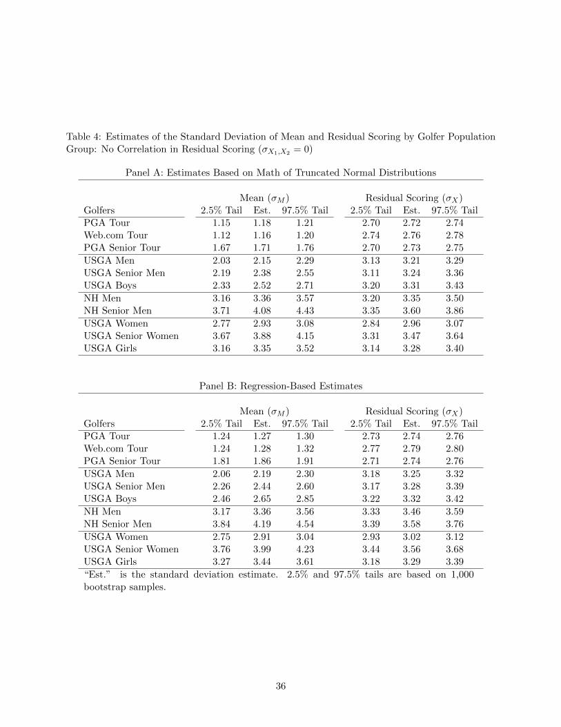
Table 4: Estimates of the Standard Deviation of Mean and Residual Scoring by Golfer PopulationGroup: No Correlation in Residual Scoring (�

X1,X2 = 0)

Panel A: Estimates Based on Math of Truncated Normal Distributions

Mean (�M

) Residual Scoring (�X

)Golfers 2.5% Tail Est. 97.5% Tail 2.5% Tail Est. 97.5% TailPGA Tour 1.15 1.18 1.21 2.70 2.72 2.74Web.com Tour 1.12 1.16 1.20 2.74 2.76 2.78PGA Senior Tour 1.67 1.71 1.76 2.70 2.73 2.75USGA Men 2.03 2.15 2.29 3.13 3.21 3.29USGA Senior Men 2.19 2.38 2.55 3.11 3.24 3.36USGA Boys 2.33 2.52 2.71 3.20 3.31 3.43NH Men 3.16 3.36 3.57 3.20 3.35 3.50NH Senior Men 3.71 4.08 4.43 3.35 3.60 3.86USGA Women 2.77 2.93 3.08 2.84 2.96 3.07USGA Senior Women 3.67 3.88 4.15 3.31 3.47 3.64USGA Girls 3.16 3.35 3.52 3.14 3.28 3.40

Panel B: Regression-Based Estimates

Mean (�M

) Residual Scoring (�X

)Golfers 2.5% Tail Est. 97.5% Tail 2.5% Tail Est. 97.5% TailPGA Tour 1.24 1.27 1.30 2.73 2.74 2.76Web.com Tour 1.24 1.28 1.32 2.77 2.79 2.80PGA Senior Tour 1.81 1.86 1.91 2.71 2.74 2.76USGA Men 2.06 2.19 2.30 3.18 3.25 3.32USGA Senior Men 2.26 2.44 2.60 3.17 3.28 3.39USGA Boys 2.46 2.65 2.85 3.22 3.32 3.42NH Men 3.17 3.36 3.56 3.33 3.46 3.59NH Senior Men 3.84 4.19 4.54 3.39 3.58 3.76USGA Women 2.75 2.91 3.04 2.93 3.02 3.12USGA Senior Women 3.76 3.99 4.23 3.44 3.56 3.68USGA Girls 3.27 3.44 3.61 3.18 3.29 3.39“Est.” is the standard deviation estimate. 2.5% and 97.5% tails are based on 1,000bootstrap samples.

36

Tab

le5:

Com

bined

Truncation

-an

dRegression-B

ased

Estim

ates

oftheStandardDeviation

ofMeanan

dResidual

Scoringby

Golfer

Pop

ulation

Group

MeanSkill(�

M

)Residual

Scoring(�

X

)Residual

Correlation

(�

X1,X

2�

2 X)

Golfers

2.5%

Tail

Est.

97.5%

Tail

2.5%

Tail

Est.

97.5%

Tail

2.5%

Tail

Est.

97.5%

Tail

PGA

Tou

r1.19

1.23

1.26

2.75

2.76

2.78

-0.018

-0.015

-0.012

Web

.com

Tou

r1.18

1.22

1.26

2.79

2.81

2.83

-0.021

-0.018

-0.014

PGA

Sen

iorTou

r1.74

1.79

1.84

2.76

2.79

2.81

-0.039

-0.033

-0.027

USGA

Men

2.06

2.17

2.29

3.19

3.26

3.34

-0.021

-0.008

0.00

8USGA

Sen

iorMen

2.23

2.41

2.57

3.19

3.31

3.41

-0.034

-0.015

0.00

8USGA

Boy

s2.40

2.59

2.77

3.26

3.37

3.48

-0.055

-0.030

-0.008

NH

Men

3.17

3.36

3.55

3.33

3.46

3.60

-0.025

0.00

20.02

9NH

Sen

iorMen

3.79

4.14

4.48

3.43

3.64

3.85

-0.087

-0.034

0.02

4USGA

Wom

en2.77

2.92

3.06

2.90

3.01

3.11

-0.015

0.00

80.03

3USGA

Sen

iorWom

en3.72

3.94

4.18

3.48

3.61

3.75

-0.063

-0.030

0.00

8USGA

Girls

3.22

3.40

3.56

3.22

3.34

3.45

-0.055

-0.029

-0.003

“Est.”

isthestan

darddeviation

estimate.

2.5%

and97

.5%

tailsarebased

on1,00

0boo

tstrap

samples.

37

Tab

le6:

Com

bined

Truncation

-an

dRegression-B

ased

Estim

ates

oftheStandardDeviation

ofMeanan

dResidual

Scoringby

Professional

GolferGroup/Tim

ePeriod

MeanSkill(�

M

)Residual

Scoring(�

X

)Golfers

Period

NEvents

2.5%

Tail

Est.

97.5%

Tail

2.5%

Tail

Est.

97.5%

Tail

PGA

Tou

r19

83-86

143

1.48

1.53

1.58

2.74

2.77

2.80

1987

-90

141

1.50

1.55

1.61

2.71

2.74

2.77

1991

-94

142

1.41

1.47

1.52

2.73

2.76

2.79

1995

-98

149

1.36

1.41

1.46

2.71

2.74

2.77

1999

-02

159

1.36

1.42

1.46

2.70

2.72

2.75

2003

-06

160

1.23

1.29

1.34

2.75

2.78

2.80

2007

-10

164

1.11

1.17

1.22

2.72

2.75

2.78

2011

-14

154

1.09

1.15

1.21

2.74

2.77

2.80

Web

.com

Tou

r19

90-93

119

1.99

2.04

2.10

2.83

2.87

2.90

1994

-97

116

1.68

1.74

1.80

2.81

2.84

2.87

1998

-01

118

1.36

1.42

1.48

2.73

2.77

2.80

2002

-05

115

1.23

1.29

1.37

2.80

2.83

2.86

2006

-09

116

1.19

1.26

1.32

2.77

2.80

2.83

2010

-14

770.95

1.04

1.12

2.75

2.79

2.83

PGA

Sen

iorTou

r19

85-88

104

1.88

1.96

2.04

2.68

2.73

2.78

1989

-92

135

1.79

1.86

1.92

2.70

2.75

2.79

1993

-96

154

1.85

1.91

1.97

2.75

2.79

2.83

1997

-00

156

1.77

1.83

1.89

2.75

2.79

2.83

2001

-04

132

1.78

1.85

1.92

2.78

2.81

2.86

2005

-08

110

1.72

1.79

1.86

2.73

2.77

2.81

2009

-14

761.61

1.71

1.79

2.71

2.77

2.82

DatafortheWeb

.com

Tou

rexcludes

2012

,an

dthereareon

lytw

oevents

included

in20

11.DataforthePGA

Sen

iorTou

rexcludes

2011

and20

12,an

dthereareon

ly4events

included

in20

10.“E

st.”

isthestan

dard

deviation

estimate.

2.5%

and97

.5%

tailsarebased

on1,00

0boo

tstrap

samples.

38