United States Environmental Protection Agency

Measuring Progress through 2003

80 84 86 88 90 92 94 96 98 00

8-H

ou

r O

zon

e

.00

0.05

0.10

0.15

0.20

0282

Mean

The Ozone Report

1980–2003: -21%

National Standard

EPA 454/ K-04-001

April 2004

The Ozone ReportMeasuring Progress through 2003

Contract No. 68-D-02-065 Work Assignment No. 2-01

U.S. Environmental Protection Agency Office of Air Quality Planning and Standards Emissions, Monitoring, and Analysis Division

Research Triangle Park, North Carolina

Contents

Introduction . . . . . . . . . . . . . . . . . . . . . . . . . . . . . . . . . . . . . . . . . . . 2

A Look at 2003 . . . . . . . . . . . . . . . . . . . . . . . . . . . . . . . . . . . . . . . . . 4

Measuring Progress . . . . . . . . . . . . . . . . . . . . . . . . . . . . . . . . . 8

A Closer Look . . . . . . . . . . . . . . . . . . . . . . . . . . . . . . . . . . . . . . . . . 11

Ozone by EPA Region . . . . . . . . . . . . . . . . . . . . . . . . . . . . . . . 11

Meteorological Adjustment . . . . . . . . . . . . . . . . . . . . . . . . . . 13

Emission Trends by EPA Region . . . . . . . . . . . . . . . . . . . . . . . 14

A New Look at Patterns in Ozone Trends. . . . . . . . . . . . . . . . 15

National Parks and Other Federal Lands . . . . . . . . . . . . . . . . 16

Looking Toward the Future . . . . . . . . . . . . . . . . . . . . . . . . . . . . . . 17

Summary . . . . . . . . . . . . . . . . . . . . . . . . . . . . . . . . . . . . . . . . . . . . . 18

The Ozone Report: Measuring Progress through 2003

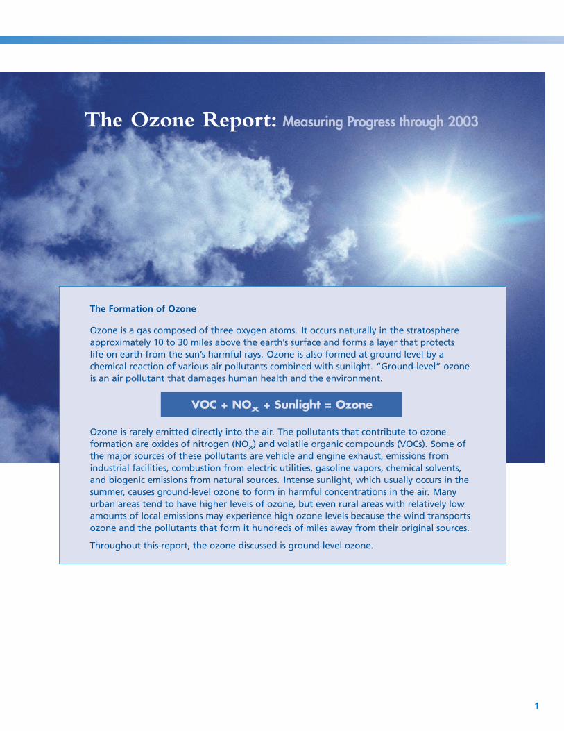
The Formation of Ozone

is an air pollutant that damages human health and the environment.

VOC + NOx + Sunlight = Ozone

formation are oxides of nitrogen (NOxthe major sources of these pollutants are vehicle and engine exhaust, emissions from industrial facilities, combustion from electric utilities, gasoline vapors, chemical solvents,

urban areas tend to have higher levels of ozone, but even rural areas with relatively low amounts of local emissions may experience high ozone levels because the wind transports ozone and the pollutants that form it hundreds of miles away from their original sources.

Throughout this report, the ozone discussed is ground-level ozone.

Ozone is a gas composed of three oxygen atoms. It occurs naturally in the stratosphere approximately 10 to 30 miles above the earth’s surface and forms a layer that protects life on earth from the sun’s harmful rays. Ozone is also formed at ground level by a chemical reaction of various air pollutants combined with sunlight. “Ground-level” ozone

Ozone is rarely emitted directly into the air. The pollutants that contribute to ozone ) and volatile organic compounds (VOCs). Some of

and biogenic emissions from natural sources. Intense sunlight, which usually occurs in the summer, causes ground-level ozone to form in harmful concentrations in the air. Many

1

IntroductionIn 2003, ozone levels nationwide were the lowest they have been since 1980. Yet ozone continues to be a pervasive air pollution problem, affecting many areas across the country and, at times, harming millions of people, sensitive vegetation, and ecosystems. This report analyzes ozone levels in 2003, summarizes the progress we have made in reducing levels of ozone since 1980, investigates how we have made progress, and looks at our current challenges and long-term prospects for continuing to reduce ground-level ozone. This report does not provide all of the answers, but may bring us closer to understanding the ozone problem, including the links between emission reduction programs, changes in emissions and meteo-rology, and ozone air quality.

Major Findings

■ Ozone levels have decreased over the past 10 to 25 years, and these reductions resulted from emission control programs. In 2003, the improved air quality resulted mainly from favorable weather conditions and continuing reductions in emissions.

■ Ozone is at its lowest level nationally since 1980, but the downward trend is slowing. One-hour levels have been reduced by 29% and 8-hour levels by 21%. Ozone levels are still decreasing nationwide, but the rate of decrease for 8-hour levels has slowed since 1990.

■ The VOC and NOx emissions that contribute to the formation of ground-level ozone have decreased 54% and 25%, respectively, since 1970 despite significant increases in vehicle miles traveled (VMT) (155%), population (39%), energy consumption (45%), and the economy (176%). These emissions declined during the 1980s and 1990s and showed continued reductions in 2003.

■ Looking at 2003 alone, more than 100 million people lived in the 209 counties with poor ozone air quality based on the nation’s 8-hour ozone standard. Most of these counties are located in the Northeast, Mid-Atlantic, Midwest, and California, with smaller numbers of areas in the South and south-central United States.

■ The most consistent and substantial improvements in 8-hour ozone levels occurred in the Northeast and southern West Coast. In other areas, where regional transport of emissions is significant, ozone trends appear flatter, indicating the need for greater attention to sources of long-range transported pollutants.

■ Meteorologically adjusted trends in many eastern U.S. cities reveal interesting patterns in similar ozone behavior. Many eastern cities exhibited increases in ozone levels during the mid-1990s followed by improvements since the late 1990s.

■ Improvements in eastern ozone air quality since the mid-1990s coincide with continued decreases in VOCs together with NOx emission reductions from the Acid Rain Program and vehicle emis-sion reduction programs. EPA recently proposed rules to reduce transported precursors of ozone and particulate pollution from stationary sources. These rules, along with rules on vehicles and off-road engines, will provide additional NOx

emission reductions.

■ Since 1990, most eastern national parks and other federal lands experienced generally improving ozone air quality. However, air quality in western parks appeared to degrade. Ozone trends in eastern national parks/federal lands appear to closely track air quality changes in nearby urban areas.

■ Over the next 10 to 15 years, scheduled regional emission reductions are expected to result in significantly fewer areas with unhealthy ozone. However, in several highly populated sections of the country, supplemental local emission control measures will be needed to attain the national air quality standards for ozone. Existing emission control measures are not expected to achieve attainment in those areas even as late as 2015.

2

significant decreases in lung function, inflammation of the airways, and increased respiratory symptoms, such as cough and pain when taking a

leading to increased medication use and increased hospital admissions and

ozone exposure because they often spend a large part of the summer

who are active outdoors (e.g., some outdoor workers) and individuals with lung diseases such as asthma and chronic obstructive pulmonary disease. In addition, long-term exposure to moderate levels of ozone may cause permanent changes in lung structure, leading to premature aging of the lungs and worsening of chronic lung disease.

agricultural crop and commercial forest yields, reduced growth and surviv-ability of tree seedlings, and increased plant susceptibility to disease, pests,

level ozone injury to trees and plants can lead to a decrease in the natural beauty of our national parks and recreation areas.

Ambient Air Quality Standards (NAAQS) for ozone by establishing 8-hour

standards are met when the expected number of days per calendar year with maximum hourly average concentrations above 0.12 ppm is equal to

the annual fourth highest daily maximum 8-hour average concentration

after an area is designated under the 8-hour standards.

Health and Ecological Effects of Ozone

Exposure to ozone has been linked to a number of health effects, including

deep breath. Exposure can also aggravate lung diseases such as asthma,

emergency room visits. Active children are the group at highest risk from

playing outdoors. Children are also more likely to have asthma, which may be aggravated by ozone exposure. Other at-risk groups include adults

Ozone also affects vegetation and ecosystems, leading to reductions in

and other environmental stresses (e.g., harsh weather). In long-lived species, these effects may become evident only after several years or even decades and may result in long-term effects on forest ecosystems. Ground-

The National Ozone Standards

In 1997, EPA revised the primary (health) and secondary (welfare) National

standards. One-hour standards have been in place since 1979. The 1-hour

or less than 1. The 8-hour standards are met when the 3-year average of

is less than 0.08 ppm. EPA expects to revoke the 1-hour standards 1 year

3

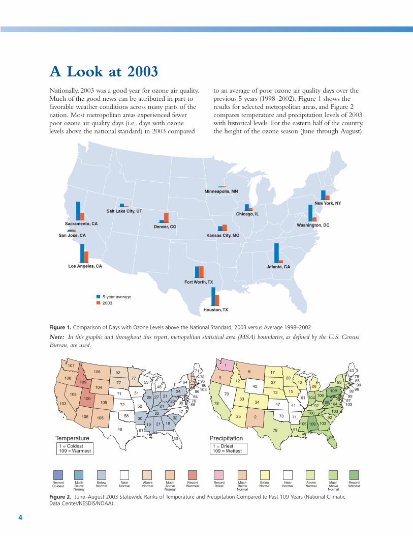
A Look at 2003Nationally, 2003 was a good year for ozone air quality. Much of the good news can be attributed in part to favorable weather conditions across many parts of the nation. Most metropolitan areas experienced fewer poor ozone air quality days (i.e., days with ozone levels above the national standard) in 2003 compared

to an average of poor ozone air quality days over the previous 5 years (1998–2002). Figure 1 shows the results for selected metropolitan areas, and Figure 2 compares temperature and precipitation levels of 2003 with historical levels. For the eastern half of the country, the height of the ozone season (June through August)

2003

5-year average

San Jose, CA

Los Angeles, CA

Salt Lake City, UT

Sacramento, CA

Houston, TX

Atlanta, GA

Kansas City, MO

Minneapolis, MN

Chicago, IL

New York, NY

Washington, DC

Fort Worth, TX

Denver, CO

Figure 1. Comparison of Days with Ozone Levels above the National Standard, 2003 versus Average 1998–2002.

Note: In this graphic and throughout this report, metropolitan statistical area (MSA) boundaries, as defined by the U.S. Census Bureau, are used.

107

108 109

106

103

105

105

106

92

104

109

77

30

52

53 77

48

58

72

71 51

22

21

31

68 76 64 86 103

86 95

71

27

78

48

21

61 19

32

47

34

39

64

26

53

18

28

1

5 12

6

70

78

25

34

2

17

42

33

27

71

41

12 20

78

73

47

13 15

100

97

106

103 97 99 92 98

90 65

43

104

78

28

109 91

105

92

103

109

104

93

109

105

103

61 108

Precipitation 1 = Coldest 1 = Driest

109 = Wettest

Temperature

109 = Warmest

Record Much Below Near Above Much Record Record Much Below Near Above Much Record Coldest Below Normal Normal Normal Above Warmest Driest Below Normal Normal Normal Above Wettest

Normal Normal Normal Normal

Figure 2. June–August 2003 Statewide Ranks of Temperature and Precipitation Compared to Past 109 Years (National Climatic Data Center/NESDIS/NOAA).

4

was cooler and wetter than normal; therefore, it was less conducive to the formation of ozone than in past years. Despite being warmer than normal between June and August, California experienced a wetter-than-normal summer, which likely contributed to lower ozone levels. Some areas, such as Denver, where the weather in 2003 was warmer and drier than usual, had more poor air quality days in 2003 than they did on average during each of the previous 5 years.

Not only were weather conditions generally good last year, but emissions of ozone precursors were also lower in 2003. Trends show that VOCs and NOx, the pollutants that contribute to ozone formation, were at their lowest levels since 1970 (see “Measuring Progress” on page 8). Determining exactly how much

Number of Counties Above the Level of the 1-hour NAAQS

94 100

46 49

98

38

of the improvement in ozone air quality is a result of weather conditions rather than lower emissions is difficult because the formation of ozone is such a complex process. This question is explored further in later sections of this report.

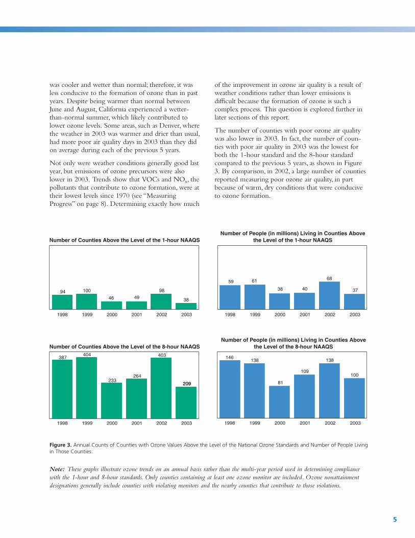
The number of counties with poor ozone air quality was also lower in 2003. In fact, the number of coun-ties with poor air quality in 2003 was the lowest for both the 1-hour standard and the 8-hour standard compared to the previous 5 years, as shown in Figure 3. By comparison, in 2002, a large number of counties reported measuring poor ozone air quality, in part because of warm, dry conditions that were conducive to ozone formation.

Number of People (in millions) Living in Counties Above the Level of the 1-hour NAAQS

59 61

38 40

68

37

1998 1999 2000 2001 2002 2003 1998 1999 2000 2001 2002 2003

Number of People (in millions) Living in Counties Above Number of Counties Above the Level of the 8-hour NAAQS the Level of the 8-hour NAAQS

387 404

233 264

403

209

146 138

81

109

138

100

209

1998 1999 2000 2001 2002 2003 1998 1999 2000 2001 2002 2003

Figure 3. Annual Counts of Counties with Ozone Values Above the Level of the National Ozone Standards and Number of People Living in Those Counties.

Note: These graphs illustrate ozone trends on an annual basis rather than the multi-year period used in determining compliance with the 1-hour and 8-hour standards. Only counties containing at least one ozone monitor are included. Ozone nonattainment designations generally include counties with violating monitors and the nearby counties that contribute to those violations.

5

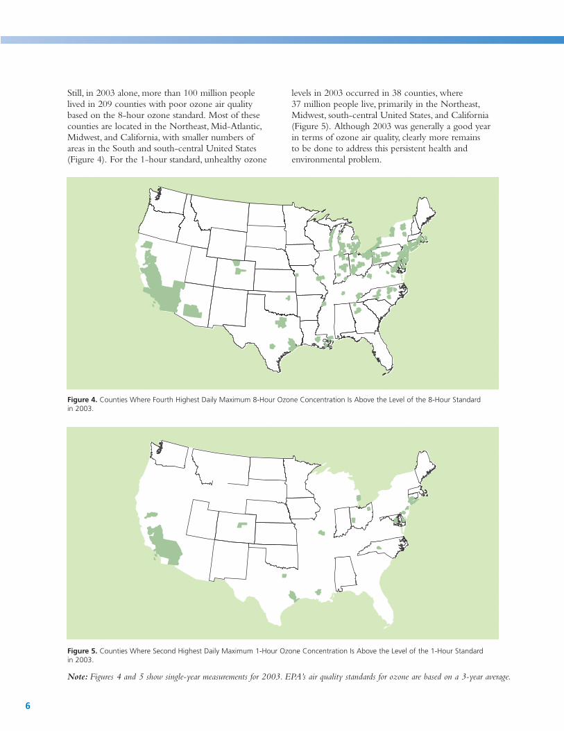
Still, in 2003 alone, more than 100 million people lived in 209 counties with poor ozone air quality based on the 8-hour ozone standard. Most of these counties are located in the Northeast, Mid-Atlantic, Midwest, and California, with smaller numbers of areas in the South and south-central United States (Figure 4). For the 1-hour standard, unhealthy ozone

levels in 2003 occurred in 38 counties, where 37 million people live, primarily in the Northeast, Midwest, south-central United States, and California (Figure 5). Although 2003 was generally a good year in terms of ozone air quality, clearly more remains to be done to address this persistent health and environmental problem.

Figure 4. Counties Where Fourth Highest Daily Maximum 8-Hour Ozone Concentration Is Above the Level of the 8-Hour Standard in 2003.

Figure 5. Counties Where Second Highest Daily Maximum 1-Hour Ozone Concentration Is Above the Level of the 1-Hour Standard in 2003.

Note: Figures 4 and 5 show single-year measurements for 2003. EPA’s air quality standards for ozone are based on a 3-year average.

6

7

Attainment or Unclassifiable Areas (2,668 counties)

Nonattainment Areas (432 entire counties)

Nonattainment Areas (42 partial counties)

Trends in ozone concentrations can be difficult to discern because

of the year-to-year variability of the data. By using a rolling 3-year

time period, we can smooth out the “peaks” and “valleys” in the

trend, making it easier to read without changing the overall trend

statistic. Three years is consistent with the 3-year period used to

assess compliance with the ozone standards. For the 1-hour trends

in this report, we use the fourth highest daily maximum over a

3-year period to be consistent with the 1-hour ozone standard. For

the 8-hour trends in this report, we use a 3-year average of the

fourth highest daily maximum in each year to be consistent with

the 8-hour ozone standard.

The 3-year statistic is assigned to the last year in each 3-year

period. For example, 1990 is based on 1988–1990, and 2003 is

based on 2001–2003. Thus, when endpoint comparisons are used

in this report to describe long-term changes (1980–2003 or

1990–2003), they are based on the first 3-year period and the

last 3-year period.

80 84 86 88 90 92 94 96 98 00

Con

cent

ratio

n, p

pm

0.00

0.05

0.10

0.15

0.20

0282

Year-to-year Rolling

Year-to-Year Versus Rolling AverageNational 8-Hour Ozone Trends, 1980–2003

On April 15, 2004, EPA identified, or designated, areas as

“attainment” or “nonattainment” for the more protective

national air quality standard for 8-hour ozone. EPA designates

an area as nonattainment if it has violated the national 8-hour

ozone standard (assessed over a 3-year period) or has contributed

to violations of this standard. The designations take effect on

June 15, 2004. They are a crucial first step in state, tribal, and

local governments’ efforts to reduce ground-level ozone.

The map below shows the 8-hour ozone nonattainment areas.

These 126 areas include 474 counties and are home to 159 million

people. These 474 counties are comprised of those with monitors

violating the standard between 2000 and 2003 and others that

contribute to the areas' ozone problems. In addition to metropol-

itan areas, some of our national parks, including Great Smoky

Mountains in Tennessee and North Carolina, Shenandoah in

Virginia, and Point Reyes National Seashore in California, are not

meeting the 8-hour ozone standards. Nonattainment areas must

take actions to improve their ozone air quality on a certain time-

line. For more details on 8-hour ozone designations, visit

www.epa.gov/ozonedesignations.

8-hour Ozone Designations

Smoothing Out the Trends

Measuring Progress

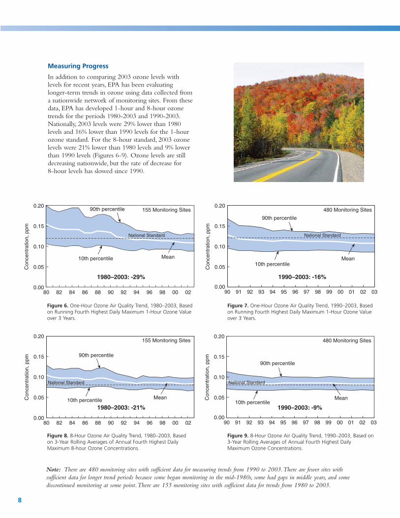
In addition to comparing 2003 ozone levels with levels for recent years, EPA has been evaluating longer-term trends in ozone using data collected from a nationwide network of monitoring sites. From these data, EPA has developed 1-hour and 8-hour ozone trends for the periods 1980-2003 and 1990-2003. Nationally, 2003 levels were 29% lower than 1980 levels and 16% lower than 1990 levels for the 1-hour ozone standard. For the 8-hour standard, 2003 ozone levels were 21% lower than 1980 levels and 9% lower than 1990 levels (Figures 6-9). Ozone levels are still decreasing nationwide, but the rate of decrease for 8-hour levels has slowed since 1990.

0.00

0.05

0.10

0.15

0.20 90th percentile

National Standard

10th percentile Mean

0.00

0.05

0.10

0.15

0.20

90th percentile

10th percentile Mean

National Standard

Con

cent

ratio

n, p

pm

155 Monitoring Sites

1980–2003: -29%

Con

cent

ratio

n, p

pm

480 Monitoring Sites

1990–2003: -16%

80 82 84 86 88 90 92 94 96 98 00 02 90 91 92 93 94 95 96 97 98 99 00 01 02 03

Figure 6. One-Hour Ozone Air Quality Trend, 1980–2003, Based on Running Fourth Highest Daily Maximum 1-Hour Ozone Value over 3 Years.

Figure 7. One-Hour Ozone Air Quality Trend, 1990–2003, Based on Running Fourth Highest Daily Maximum 1-Hour Ozone Value over 3 Years.

0.00

0.05

0.10

0.15

0.20

90th percentile

10th percentile Mean

National Standard

0.00

0.05

0.10

0.15

0.20

90th percentile

10th percentile Mean

National Standard

Con

cent

ratio

n, p

pm

480 Monitoring Sites

1990–2003: -9%

Con

cent

ratio

n, p

pm

155 Monitoring Sites

1980–2003: -21%

80 82 84 86 88 90 92 94 96 98 00 02 90 91 92 93 94 95 96 97 98 99 00 01 02 03

Figure 8. 8-Hour Ozone Air Quality Trend, 1980–2003, Based on 3-Year Rolling Averages of Annual Fourth Highest Daily Maximum 8-hour Ozone Concentrations.

Figure 9. 8-Hour Ozone Air Quality Trend, 1990–2003, Based on 3-Year Rolling Averages of Annual Fourth Highest Daily Maximum Ozone Concentrations.

Note: There are 480 monitoring sites with sufficient data for measuring trends from 1990 to 2003.There are fewer sites with sufficient data for longer trend periods because some began monitoring in the mid-1980s, some had gaps in middle years, and some discontinued monitoring at some point.There are 155 monitoring sites with sufficient data for trends from 1980 to 2003.

8

70 019580 90 96 97 98 99 00 02

-50%

0%

50%

100%

150%

200%

176%

155%

45%

39%

-54%

03

-25% NOx Emissions

Gross Domestic Product

Energy Consumption

x

VOC Emissions

Vehicle Miles Traveled

Population

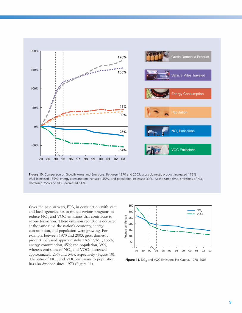
Figure 10. Comparison of Growth Areas and Emissions. Between 1970 and 2003, gross domestic product increased 176% VMT increased 155%, energy consumption increased 45%, and population increased 39%. At the same time, emissions of NOdecreased 25% and VOC decreased 54%.

Over the past 30 years, EPA, in conjunction with state and local agencies, has instituted various programs to reduce NOx and VOC emissions that contribute to ozone formation. These emission reductions occurred at the same time the nation’s economy, energy consumption, and population were growing. For example, between 1970 and 2003, gross domestic product increased approximately 176%; VMT, 155%; energy consumption, 45%; and population, 39%, whereas emissions of NOx and VOCs decreased approximately 25% and 54%, respectively (Figure 10). The ratio of NOx and VOC emissions to population has also dropped since 1970 (Figure 11).

Pou

nds

per

Per

son

350

300

250

200

150

100

50

070 9590 9996 98 00 0280 97 0301

NOx VOC

Figure 11. NOx and VOC Emissions Per Capita, 1970–2003.

9

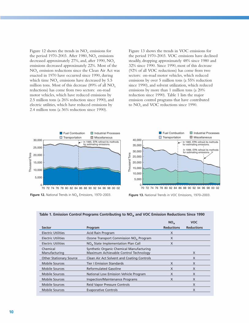
Figure 12 shows the trends in NOx emissions for the period 1970-2003. After 1980, NOx emissions decreased approximately 27%, and, after 1990, NOx

emissions decreased approximately 22%. Most of the NOx emission reductions since the Clean Air Act was enacted in 1970 have occurred since 1990, during which time NOx emissions have decreased by 5.5 million tons. Most of this decrease (89% of all NOx

reductions) has come from two sectors: on-road motor vehicles, which have reduced emissions by 2.5 million tons (a 26% reduction since 1990), and electric utilities, which have reduced emissions by 2.4 million tons (a 36% reduction since 1990).

Fuel Combustion Industrial Processes

Transportation Miscellaneous

Figure 13 shows the trends in VOC emissions for the period 1970-2003. VOC emissions have declined steadily, dropping approximately 48% since 1980 and 32% since 1990. Since 1990, most of this decrease (92% of all VOC reductions) has come from two sectors: on-road motor vehicles, which reduced emissions by over 5 million tons (a 55% reduction since 1990), and solvent utilization, which reduced emissions by more than 1 million tons (a 20% reduction since 1990). Table 1 lists the major emission control programs that have contributed to NOx and VOC reductions since 1990.

Fuel Combustion Industrial Processes

Transportation Miscellaneous 30,000 40,000

In 1985, EPA refined its methods for estimating emissions.

Tho

usan

d To

ns

10,0005,000

5,000

0 0 70 72 74 76 78 80 82 84 86 88 90 92 94 96 98 00 02 70 72 74 76 78 80 82 84 86 88 90 92 94 96 98 00 02

In 1996, EPA refined its methods for estimating emissions.

In 1985, EPA refined its methods for estimating emissions.

Figure 12. National Trends in NOx Emissions, 1970–2003. Figure 13. National Trends in VOC Emissions, 1970–2003.

35,00025,000

30,000

Tho

usan

d To

ns

20,000 25,000

20,00015,000

15,00010,000

x and VOC Emission Reductions Since 1990

NOx VOC

Sector Reductions Reductions

Electric Utilities Acid Rain Program X

Electric Utilities x Program X

Electric Utilities NOx X

Chemical Synthetic Organic Chemical Manufacturing Manufacturing X

Other Stationary Source Clean Air Act Solvent and Coating Controls X

Mobile Sources X X

Mobile Sources Reformulated Gasoline X X

Mobile Sources X X

Mobile Sources Inspection/Maintenance Programs X X

Mobile Sources X

Mobile Sources Evaporative Controls X

Table 1. Emission Control Programs Contributing to NO

Program

Ozone Transport Commission NO

State Implementation Plan Call

Maximum Achievable Control Technology

Tier I Emission Standards

National Low Emission Vehicle Program

Reid Vapor Pressure Controls

10

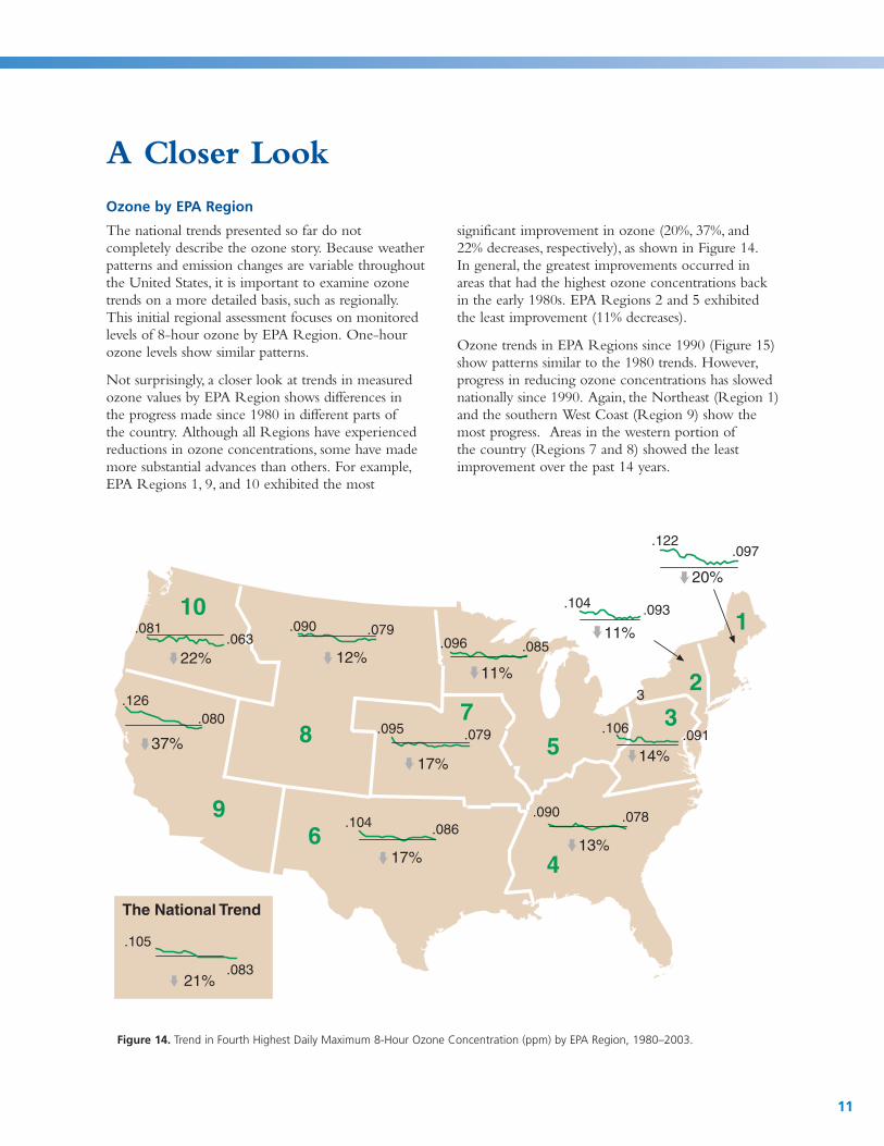
A Closer LookOzone by EPA Region

The national trends presented so far do not completely describe the ozone story. Because weather patterns and emission changes are variable throughout the United States, it is important to examine ozone trends on a more detailed basis, such as regionally. This initial regional assessment focuses on monitored levels of 8-hour ozone by EPA Region. One-hour ozone levels show similar patterns.

Not surprisingly, a closer look at trends in measured ozone values by EPA Region shows differences in the progress made since 1980 in different parts of the country. Although all Regions have experienced reductions in ozone concentrations, some have made more substantial advances than others. For example, EPA Regions 1, 9, and 10 exhibited the most

significant improvement in ozone (20%, 37%, and 22% decreases, respectively), as shown in Figure 14. In general, the greatest improvements occurred in areas that had the highest ozone concentrations back in the early 1980s. EPA Regions 2 and 5 exhibited the least improvement (11% decreases).

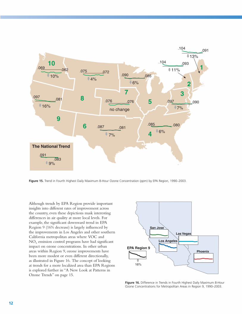
Ozone trends in EPA Regions since 1990 (Figure 15) show patterns similar to the 1980 trends. However, progress in reducing ozone concentrations has slowed nationally since 1990. Again, the Northeast (Region 1) and the southern West Coast (Region 9) show the most progress. Areas in the western portion of the country (Regions 7 and 8) showed the least improvement over the past 14 years.

.122 .097

10

9

8 7

6

5

4

3

2

1

.080 .126 3

37%

.105

.083 21%

.081 .063

22%

.090 .079

12%

.104 .086

17%

.095 .079

17%

.090 .078

13%

.096 .085

11%

.104 .093

11%

20%

.106 .091

14%

The National Trend

Figure 14. Trend in Fourth Highest Daily Maximum 8-Hour Ozone Concentration (ppm) by EPA Region, 1980–2003.

11

.104

10

9

8 7

6

5

4

3

2

1

.076 .076

.087 .081

.075 .072

.081.097

.090 .085

.104 .093

.097 .090

.085 .080

7%

no change 16%

6%

7%

11%

.091

13%

.069 .062

10%

6%

4%

.091 .083

9%

The National Trend

Figure 15. Trend in Fourth Highest Daily Maximum 8-Hour Ozone Concentration (ppm) by EPA Region, 1990–2003.

Although trends by EPA Region provide important insights into different rates of improvement across the country, even these depictions mask interesting differences in air quality at more local levels. For example, the significant downward trend in EPA Region 9 (16% decrease) is largely influenced by the improvements in Los Angeles and other southern California metropolitan areas where VOC and NOx emission control programs have had significant impact on ozone concentrations. In other urban areas within Region 9, ozone improvements have been more modest or even different directionally, as illustrated in Figure 16. The concept of looking at trends for a more localized area than EPA Regions is explored further in “A New Look at Patterns in Ozone Trends” on page 15.

Phoenix

San Jose

16%

Los Angeles

Las Vegas

EPA Region 9

Figure 16. Difference in Trends in Fourth Highest Daily Maximum 8-Hour Ozone Concentrations for Metropolitan Areas in Region 9, 1990–2003.

12

50

40

Meteorological Adjustment

Ozone is formed through complex chemical reactions of VOC and NOx emissions during periods of conducive weather conditions. Ozone is more readily formed when it is sunny and hot and the air is stag-nant. Conversely, ozone production is more limited when it is cloudy, cool, rainy, and windy. For these reasons, ozone concentrations are generally the highest during the summer.

To separate the effects of weather from those of VOC and NOx emissions, measured ozone levels can be adjusted to account for the impact of meteorology. This meteorological adjustment technique helps us understand how much of the year-to-year variability of an ozone trend is due to the weather rather than to the effects of emission control programs.

The number of summertime days above 90˚ is one of the indicators of conditions conducive to ozone formation. Figure 17 shows temperature data together with the meteorologically adjusted trends (1990–2003) for two example metropolitan areas. For these eastern cities, the meteorological adjustment generally lowers the measured ozone when the summer is relatively hot. Similarly, when the summer is cool, the adjusted value is usually increased. For Atlanta, you can see these adjustments for the hot summer of 1993 (where the meteorologically adjusted value is lower) and the cool summer of 2003 (where the adjusted ozone value is higher). These graphics help explain how meteorologically adjusted trends smooth out some of the year-to-year variability in observed ozone levels.

Bridgeport, CT 80

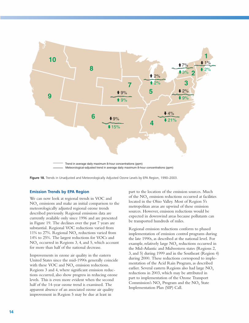
Figure 18 presents trends in meteorologically adjusted ozone levels by EPA Region from 1990 to 2003. These results are based on summertime average daily maximum 8-hour ozone and meteorological data for 35 selected eastern cities. (At the time of publication, meteorologically adjusted data for western cities were not available.) With these analyses, we can begin to look at some of the influence of meteorology on ozone. However, these analyses are based on a limited number of cities in each EPA Region, so these regional trends should not be compared directly to the regional trends presented in the previous section. Before adjusting for weather, EPA Regions 3, 4, and 6 show improving air quality, with average reductions in ozone levels of 9% to 21%. After adjusting for weather, however, each Region demonstrates a more moderate decline. The most dramatic effect of the meteorological adjustment is in Region 4, where the adjusted trend shows a 4% decrease, compared with a 21% decrease for the unadjusted trend. Region 6 shows the largest improvement, 9%, after adjusting for meteorology. Ozone levels in the midwest and central regions of the country show the same percent increase in ozone both with and without the meteorological adjustment. EPA Region 2 shows a larger increase in ozone levels after the meteorological adjustment is applied.

The current meteorological adjustment method does not reflect all of the influences of meteorology on ozone. For example, future analyses will try to better account for year-to-year variations in ozone levels due to regional transport.

Atlanta, GA 100 80

70 80 70

Num

ber

of D

ays

>90

º

Ozo

ne, p

pm

Ozo

ne, p

pm

Num

ber

of D

ays

>90

º

60 60 60

50 40 50

40 20 40

30 00 30 90 91 92 93 94 95 96 97 98 99 00 01 02 03 90 91 92 93 94 95 96 97 98 99 00 01 02 03

Unadjusted Ozone Meteorologically Adjusted Ozone

Figure 17. Number of Days Daily Maximum Temperatures Exceed 90 (bar) Compared to Unadjusted Ozone (red line) and ˚ Meteorologically Adjusted Ozone (blue line) for Bridgeport and Atlanta, 1990–2003. Ozone Concentrations are Annual Average Daily Maximum 8-Hour Values between June and August.

13

30

20

10

10

9

8

7

6

5

4

3

2

1

9%

2%

7%

3%

1%

2%

21%

4%

15%

9%

9%

9%

2%

2%

Trend in average daily maximum 8-hour concentrations (ppm) Meteorological-adjusted trend in average daily maximum 8-hour concentrations (ppm)

Figure 18. Trends in Unadjusted and Meteorologically Adjusted Ozone Levels by EPA Region, 1990–2003.

Emission Trends by EPA Region

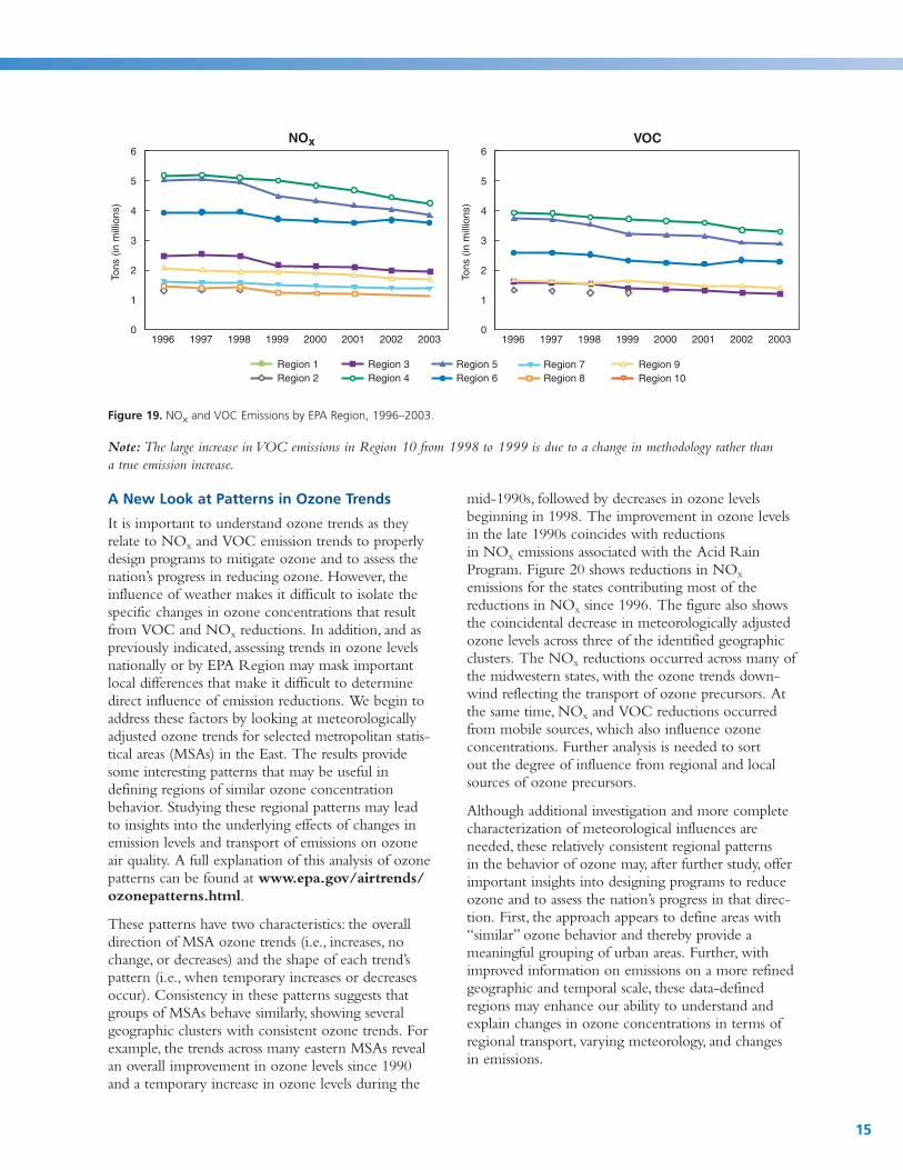
We can now look at regional trends in VOC and NOx emissions and make an initial comparison to the meteorologically adjusted regional ozone trends described previously. Regional emissions data are currently available only since 1996 and are presented in Figure 19. The declines over the past 7 years are substantial. Regional VOC reductions varied from 11% to 27%. Regional NOx reductions varied from 14% to 25%. The largest reductions for VOCs and NOx occurred in Regions 3, 4, and 5, which account for more than half of the national decrease.

Improvements in ozone air quality in the eastern United States since the mid-1990s generally coincide with these VOC and NOx emission reductions. Regions 3 and 4, where significant emission reduc-tions occurred, also show progress in reducing ozone levels. This is even more evident when the second half of the 14-year ozone trend is examined. The apparent absence of an associated ozone air quality improvement in Region 5 may be due at least in

part to the location of the emission sources. Much of the NOx emission reductions occurred at facilities located in the Ohio Valley. Most of Region 5’s metropolitan areas are upwind of these emission sources. However, emission reductions would be expected in downwind areas because pollutants can be transported hundreds of miles.

Regional emission reductions conform to phased implementation of emission control programs during the late 1990s, as described at the national level. For example, relatively large NOx reductions occurred in the Mid-Atlantic and Midwestern states (Regions 2, 3, and 5) during 1999 and in the Southeast (Region 4) during 2000. These reductions correspond to imple-mentation of the Acid Rain Program, as described earlier. Several eastern Regions also had large NOx

reductions in 2003, which may be attributed in part to implementation of the Ozone Transport Commission’s NOx Program and the NOx State Implementation Plan (SIP) Call.

14

4

3

2

Tons

(in

mill

ions

)

NOx VOC 6 6

5 5

Tons

(in

mill

ions

)

4

3

2

1 1

0 0 1996 1997 1998 1999 2000 2001 2002 2003 1996 1997 1998 1999 2000 2001 2002 2003

Region 1 Region 3 Region 5 Region 7 Region 9 Region 2 Region 4 Region 6 Region 8 Region 10

Figure 19. NOx and VOC Emissions by EPA Region, 1996–2003.

Note: The large increase in VOC emissions in Region 10 from 1998 to 1999 is due to a change in methodology rather than a true emission increase.

A New Look at Patterns in Ozone Trends

It is important to understand ozone trends as they relate to NOx and VOC emission trends to properly design programs to mitigate ozone and to assess the nation’s progress in reducing ozone. However, the influence of weather makes it difficult to isolate the specific changes in ozone concentrations that result from VOC and NOx reductions. In addition, and as previously indicated, assessing trends in ozone levels nationally or by EPA Region may mask important local differences that make it difficult to determine direct influence of emission reductions. We begin to address these factors by looking at meteorologically adjusted ozone trends for selected metropolitan statis-tical areas (MSAs) in the East. The results provide some interesting patterns that may be useful in defining regions of similar ozone concentration behavior. Studying these regional patterns may lead to insights into the underlying effects of changes in emission levels and transport of emissions on ozone air quality. A full explanation of this analysis of ozone patterns can be found at www.epa.gov/airtrends/ ozonepatterns.html.

These patterns have two characteristics: the overall direction of MSA ozone trends (i.e., increases, no change, or decreases) and the shape of each trend’s pattern (i.e., when temporary increases or decreases occur). Consistency in these patterns suggests that groups of MSAs behave similarly, showing several geographic clusters with consistent ozone trends. For example, the trends across many eastern MSAs reveal an overall improvement in ozone levels since 1990 and a temporary increase in ozone levels during the

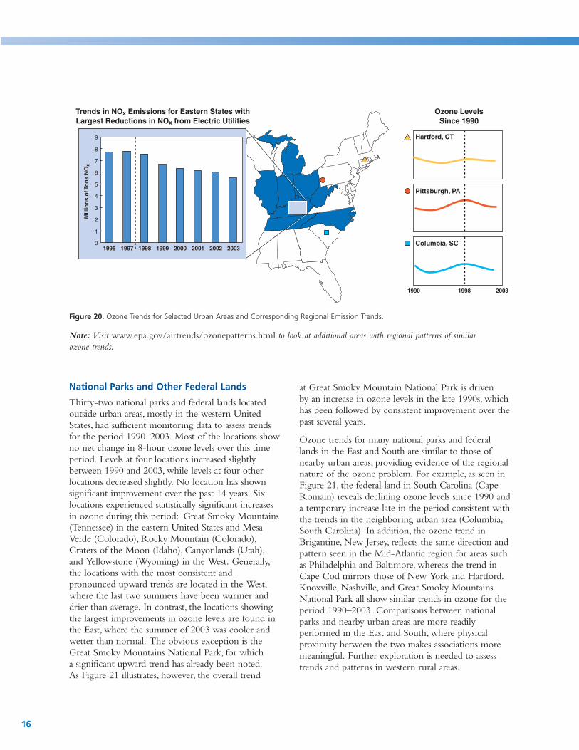
mid-1990s, followed by decreases in ozone levels beginning in 1998. The improvement in ozone levels in the late 1990s coincides with reductions in NOx emissions associated with the Acid Rain Program. Figure 20 shows reductions in NOx

emissions for the states contributing most of the reductions in NOx since 1996. The figure also shows the coincidental decrease in meteorologically adjusted ozone levels across three of the identified geographic clusters. The NOx reductions occurred across many of the midwestern states, with the ozone trends down-wind reflecting the transport of ozone precursors. At the same time, NOx and VOC reductions occurred from mobile sources, which also influence ozone concentrations. Further analysis is needed to sort out the degree of influence from regional and local sources of ozone precursors.

Although additional investigation and more complete characterization of meteorological influences are needed, these relatively consistent regional patterns in the behavior of ozone may, after further study, offer important insights into designing programs to reduce ozone and to assess the nation’s progress in that direc-tion. First, the approach appears to define areas with “similar” ozone behavior and thereby provide a meaningful grouping of urban areas. Further, with improved information on emissions on a more refined geographic and temporal scale, these data-defined regions may enhance our ability to understand and explain changes in ozone concentrations in terms of regional transport, varying meteorology, and changes in emissions.

15

Trends in NOx Emissions for Eastern States with Largest Reductions in NOx from Electric Utilities

0

1

2

3

4

5

6

7

8

9

1996 1997 1998 1999 2000 2001 2002 2003

x M

illio

ns

of T

on

s N

O

1990 1998 2003

Figure 20. Ozone Trends for Selected Urban Areas and Corresponding Regional Emission Trends.

Note: Visit www.epa.gov/airtrends/ozonepatterns.html to look at additional areas with regional patterns of similar

Ozone Levels Since 1990

Columbia, SC

Pittsburgh, PA

Hartford, CT

ozone trends.

National Parks and Other Federal Lands

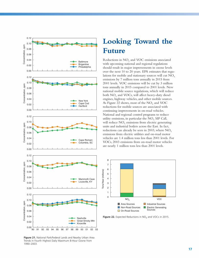
Thirty-two national parks and federal lands located outside urban areas, mostly in the western United States, had sufficient monitoring data to assess trends for the period 1990–2003. Most of the locations show no net change in 8-hour ozone levels over this time period. Levels at four locations increased slightly between 1990 and 2003, while levels at four other locations decreased slightly. No location has shown significant improvement over the past 14 years. Six locations experienced statistically significant increases in ozone during this period: Great Smoky Mountains (Tennessee) in the eastern United States and Mesa Verde (Colorado), Rocky Mountain (Colorado), Craters of the Moon (Idaho), Canyonlands (Utah), and Yellowstone (Wyoming) in the West. Generally, the locations with the most consistent and pronounced upward trends are located in the West, where the last two summers have been warmer and drier than average. In contrast, the locations showing the largest improvements in ozone levels are found in the East, where the summer of 2003 was cooler and wetter than normal. The obvious exception is the Great Smoky Mountains National Park, for which a significant upward trend has already been noted. As Figure 21 illustrates, however, the overall trend

at Great Smoky Mountain National Park is driven by an increase in ozone levels in the late 1990s, which has been followed by consistent improvement over the past several years.

Ozone trends for many national parks and federal lands in the East and South are similar to those of nearby urban areas, providing evidence of the regional nature of the ozone problem. For example, as seen in Figure 21, the federal land in South Carolina (Cape Romain) reveals declining ozone levels since 1990 and a temporary increase late in the period consistent with the trends in the neighboring urban area (Columbia, South Carolina). In addition, the ozone trend in Brigantine, New Jersey, reflects the same direction and pattern seen in the Mid-Atlantic region for areas such as Philadelphia and Baltimore, whereas the trend in Cape Cod mirrors those of New York and Hartford. Knoxville, Nashville, and Great Smoky Mountains National Park all show similar trends in ozone for the period 1990–2003. Comparisons between national parks and nearby urban areas are more readily performed in the East and South, where physical proximity between the two makes associations more meaningful. Further exploration is needed to assess trends and patterns in western rural areas.

16

0.00

0.02

0.06

0.04

0.00

0.02

0.10

0.06

0.12

0.04

0.08

Baltimore

Philadelphia

Con

cent

ratio

n, p

pm

Brigantine

Looking Toward the Future Reductions in NOx and VOC emissions associated with upcoming national and regional regulationsshould result in major improvements in ozone levels

0.00

0.02

0.10

0.06

0.12

0.04

0.08

Cape CodCon

cent

ratio

n, p

pm

New York

Hartford

over the next 10 to 20 years. EPA estimates that regu-lations for mobile and stationary sources will cut NOx

emissions by 7 million tons annually in 2015 from 2001 levels. VOC emissions will be cut by 3 million tons annually in 2015 compared to 2001 levels. New national mobile source regulations, which will reduce both NOx and VOCs, will affect heavy-duty diesel engines, highway vehicles, and other mobile sources.As Figure 22 shows, most of the NOx and VOC reductions for mobile sources are associated with

Con

cent

ratio

n, p

pm

Cape Romain Columbia, SC

Mammoth Cave Louisville, KY

Tons

/Yea

r (m

illio

ns)

0.12

0.10

0.08

0.06

0.04

0.02 are nearly 1 million tons less than 2001 levels.

0.00

0.12

80.10

7 0.08

continuing improvements in on-road vehicles. National and regional control programs to reduce utility emissions, in particular the NOx SIP Call, will reduce NOx emissions from electric generating units and industrial boilers across the East. In fact, reductions can already be seen in 2003, where NOx

emissions from electric utilities and on-road motor vehicles are 1.4 million tons less than 2001 levels. For VOCs, 2003 emissions from on-road motor vehicles

Con

cent

ratio

n, p

pm

Con

cent

ratio

n, p

pm

6

5

4

3

2

1 0.12

Nashville Great Smoky Mtn Knoxville

0 NOx VOC 0.10

Area Sources Industrial Sources 0.08

Non-Road Sources Electric Generating SourcesOn-Road Sources0.06

0.04 Figure 22. Expected Reductions in NOx and VOCs in 2015.

0.02

0.00 90 91 92 93 94 95 96 97 98 99 00 01 02 03

Figure 21. National Park/Federal Lands and Nearby Urban Area Trends in Fourth Highest Daily Maximum 8-Hour Ozone from 1990–2003.

17

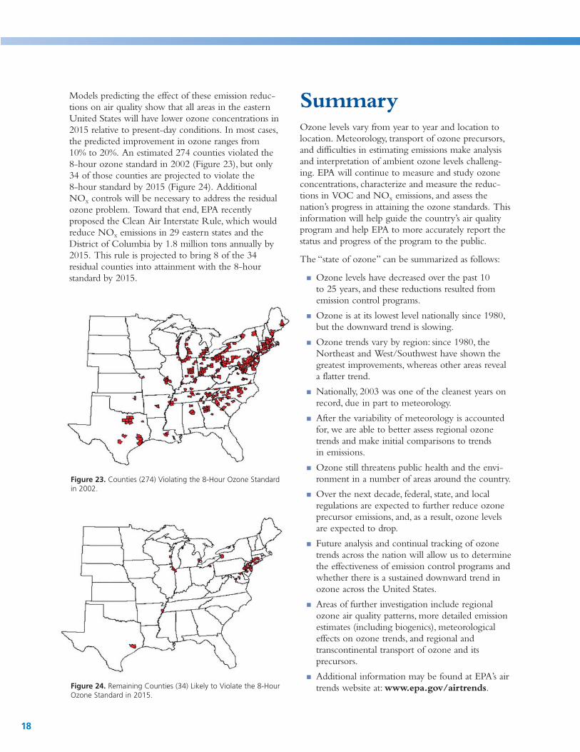
Models predicting the effect of these emission reduc-tions on air quality show that all areas in the eastern United States will have lower ozone concentrations in 2015 relative to present-day conditions. In most cases, the predicted improvement in ozone ranges from 10% to 20%. An estimated 274 counties violated the 8-hour ozone standard in 2002 (Figure 23), but only 34 of those counties are projected to violate the 8-hour standard by 2015 (Figure 24). Additional NOx controls will be necessary to address the residual ozone problem. Toward that end, EPA recently proposed the Clean Air Interstate Rule, which would reduce NOx emissions in 29 eastern states and the District of Columbia by 1.8 million tons annually by 2015. This rule is projected to bring 8 of the 34 residual counties into attainment with the 8-hour standard by 2015.

SummaryOzone levels vary from year to year and location to location. Meteorology, transport of ozone precursors, and difficulties in estimating emissions make analysis and interpretation of ambient ozone levels challeng-ing. EPA will continue to measure and study ozone concentrations, characterize and measure the reduc-tions in VOC and NOx emissions, and assess the nation’s progress in attaining the ozone standards. This information will help guide the country’s air quality program and help EPA to more accurately report the status and progress of the program to the public.

The “state of ozone” can be summarized as follows:

■ Ozone levels have decreased over the past 10 to 25 years, and these reductions resulted from

Figure 23. Counties (274) Violating the 8-Hour Ozone Standard in 2002.

Figure 24. Remaining Counties (34) Likely to Violate the 8-Hour Ozone Standard in 2015.

emission control programs.

■ Ozone is at its lowest level nationally since 1980, but the downward trend is slowing.

■ Ozone trends vary by region: since 1980, the Northeast and West/Southwest have shown the greatest improvements, whereas other areas reveal a flatter trend.

■ Nationally, 2003 was one of the cleanest years on record, due in part to meteorology.

■ After the variability of meteorology is accounted for, we are able to better assess regional ozone trends and make initial comparisons to trends in emissions.

■ Ozone still threatens public health and the envi-ronment in a number of areas around the country.

■ Over the next decade, federal, state, and local regulations are expected to further reduce ozone precursor emissions, and, as a result, ozone levels are expected to drop.

■ Future analysis and continual tracking of ozone trends across the nation will allow us to determine the effectiveness of emission control programs and whether there is a sustained downward trend in ozone across the United States.

■ Areas of further investigation include regional ozone air quality patterns, more detailed emission estimates (including biogenics), meteorological effects on ozone trends, and regional and transcontinental transport of ozone and its precursors.

■ Additional information may be found at EPA’s air trends website at: www.epa.gov/airtrends.

18

Clean Air Act

MSA

NOx

ppm

SIP State Implementation Plan

VMT

For Further Information

Acronyms

CAA

EPA U.S. Environmental Protection Agency

MACT maximum achievable control technology

metropolitan statistical area

NAAQS National Ambient Air Quality Standards

oxides of nitrogen

parts per million

vehicle miles traveled

VOC volatile organic compound

Reference

U.S. Environmental Protection Agency. 1996. Air Quality Criteria for Ozone and Related Photochemical Oxidants. EPA/600/P-93/004a-cF. Research Triangle Park, NC: U.S. Environmental Protection Agency.

Web Sites

Bureau of Economic Analysis: www.bea.gov

Bureau of Transportation Statistics: www.bts.gov

Clean Air Interstate Rule: www.epa.gov/interstateairquality

Detailed Information of Air Pollution Trends: www.epa.gov/airtrends

Energy Information Administration: www.eia.doe.gov

Formation of Ozone: www.epa.gov/air/urbanair/ozone/what.html

Health and Ecological Effects: www.epa.gov/airnow/health/smog1.html#3 www.epa.gov/air/urbanair/ozone/hlth.html

National Park Service: www.nps.gov

Office of Air and Radiation: www.epa.gov/oar

Office of Air Quality Planning and Standards: www.epa.gov/oar/oaqps

Office of Atmospheric Programs: www.epa.gov/air/oap.html

Office of Radiation and Indoor Air: www.epa.gov/air/oria.html

Office of Transportation and Air Quality: www.epa.gov/otaq

Online Air Quality Data: www.epa.gov/air/data/index.html

Ozone Depletion: www.epa.gov/ozone

Ozone Designations: www.epa.gov/ozonedesignations

Real-Time Air Quality Maps and Forecasts: www.epa.gov/airnow

Regional Patterns in Ozone: www.epa.gov/airtrends/ozonepatterns.html

Westar: www.westar.org/downloads.html

U.S. Census Bureau: www.census.gov

19