the origins of euler's variational...
TRANSCRIPT

The Origins of Euler's Variational Calculus
CRAIG G. FRASER
Communicated by H. Bos
1. Introduction
The calculus of variations was established as a distinct branch of analysis with the publication in 1744 of EULER'S Methodus inveniendi curvas lineas. EULER succeeded in formulating the variational problem in a general way, in identify- ing standard equational forms of solution and in providing a systematic tech- nique to derive them. His work included a classification of the major types of problems and was illustrated by a wide range of examples.
EULER'S treatise was the culmination of a line of research that had begun a half-century earlier with the publication of two papers by JAKOB BERNOULLI in the Acta eruditorum. BERNOULLI'S pioneering researches were continued by his brother JOHANN and by the English mathematician BROOK TAYLOR. EULER'S initial investigations in the 1730s began from a study of the work of these men.
Ironically EULER'S entire approach to the subject would be set aside with the appearance of LA~RAN~E'S &method in the 1750s. This method, which very quickly became standard, involved a variational process that was fundamentally different from EULER'S and that established the subject along new and different lines. There is a family resemblance shared by the techniques of the BE~NOtJLLIS, TAYLOR and EULER that distinguish them from those employed in the post- Lagrangian stage of the subject.
From a larger historical perspective it is clear that the Methodus inveniendi capped and completed the first phase in the development of the calculus of variations. The treatise was nevertheless by no means a straightforward product of earlier research. In its basic organization and direction it represented a sub- stantial break with the then established tradition, including EuL~R's own pre- vious work in the subject.
The present paper is concerned to identify some significant characteristics of the BERNOULLIS' and TAYLOR'S theory and to document the substantial achieve- ments of EULER'S variational calculus that preceded the Methodus inveniendi. The intent is to illuminate the earlier developments and to explain how and for what reasons the subject assumed the form that it did in the treatise of 1744. In order to orient the discussion and to provide a basis of reference we begin by laying out in summary the salient points of the subject as it is developed in the Methodus inveniendi. We then turn to an examination of the BERNOULLIS' re- search, with consideration of the ways in which their approach was similar to
104 C.G. FRASER
and differed from EULER'S. A study of TAVLOR'S solution to the isoperimetric problem will reveal its special significance in the background to his investiga- tions. Finally, we discuss in some detail EULER'S variational papers of 1738 and 1741 that were published as memoirs of the St. Petersburg Academy of Science. We conclude with some reflections on the early history of the calculus of variations.
2. Euler's Theory of 1744
2.1 The problems considered by EULER in the Methodus inveniendi fall naturally into three groups.
I. Presented in Chapter 2, these problems are the most basic ones, in which no side condition or special relation among the variables is assumed.
II. Presented in Chapter 3, these involve certain variational integrals in which a variable appears in the integrand that is connected to the other variables of the problem by means of a differential equation. In the modern subject this problem is an instance of the very general "problem of LAGRANGE".
IlI. Presented in Chapter 5, these involve a side condition that is formulated in terms of a definite integral. The isoperimetric problem is the classical repre- sentative of this class of problems.
EULER'S theory is based on his derivation of the variational equations for these three classes of problems.
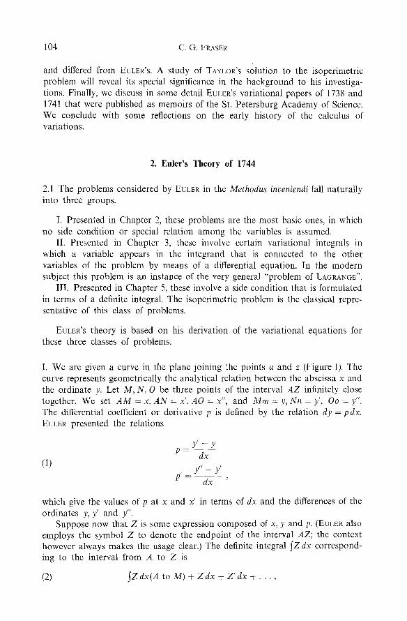
I. We are given a curve in the plane joining the points a and z (Figure 1). The curve represents geometrically the analytical relation between the abscissa x and the ordinate y. Let M, N, O be three points of the interval A Z infinitely close together. We set A M = x, A N = x', A O = x", and M m = y, N n = y', Oo = y".
The differential coefficient or derivative p is defined by the relation dy = p dx.
EULEe presented the relations
(1)
y l __ y
P - dx
y,, _ y' pr__
dx
which give the values of p at x and x' in terms of dx and the differences of the ordinates y, y' and y".
Suppose now that Z is some expression composed of x, y and p. (EULER also employs the symbol Z to denote the endpoint of the interval AZ; the context however always makes the usage clear.) The definite integral ~Z dx correspond- ing to the interval from A to Z is
(2) ~ Z d x ( A to M) + Z d x 4- Z ' d x + . . . ,

The Origins of Euler's Variational Calculus 105
A. ~x~ K L ~ N O P Q R 5
7~
7-
Figure 1.
where Z, Z ' , . . . are the values of Z at x, y, p; x', y', p'; . . . . Suppose the given curve joining a to z is such that (2) is a maximum or minimum. Increase the ordinate y' by the infinitely small quantity nv, obtaining in this way a compari- son curve amvoz. The change in the value of the integral calculated along the given and comparison curves must by hypothesis be zero. The only part of the integral that is affected by varying y' is Z dx + Z'dx. EULER wrote
dZ = M d x + Ndy + Pdp (3)
dZ ' = M'dx + N'dy ' + Udp ' .
He proceeded to interpret the differentials in (3) as the infinitesimal changes in Z , Z ' , x , y , y ' , p , p ' that result when y' is increased by nv. Evidently dx = O, dy = 0 and dy' = nv. From (1) we see that dp and dp' equal nv/dx and - nv/dx respectively. Hence (3) becomes
tz~ dZ = P ' ~
(4) dx n v
dZ ' = N " n v - P " - - dx
Thus the total change in ~ Z d x (A to Z) equals (dZ + dZ ' )dx = n v . ( P + N ' d x - P ' ) . This expression must be equated to zero. We set
P ' - P = dP and replace N ' by N. We therefore obtain N d x - dP or
(5) N - --dn = O , dx
as the final equation for the curve. In later mathematics (5) would be written as O f / O y - d(Of/@')/dx = 0 and
become widely known as the EULER or EULER-LAGRANGE equation of the varia- tional problem.
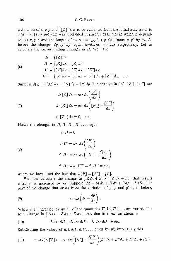
II. In Chapter 3 EULER moved to a new set of examples. Here it is typically required to render extreme an integral of the form y Zdx, in which Z is now a function of x, y, p = dy/dx and a new v a r i a b l e / / = y [Z] dx, where [Z] itself is
106 C.G. FRASER
a function of x, y, p and ~ [Z] dx is to be evaluated from the initial abscissa A to A M = x. (This problem was motivated in part by examples in which Z depend-
ed on x, y, p and the length of path s = ~o , f i + f d x . ) Increase y' by nv. As before the changes dp, dy', dp' equal nv/dx, n v , - nv/dx respectively. Let us calculate the corresponding changes in 17. We have
17 = ~ [ z ] dx
/7' = ~ [Z] dx + [Z] dx (6)
17"= ~ [z] dx + [z] dx + [z'] dx
17" = ~[Z] dx + [Z] dx + [Z'] dx + [Z"] dx, etc.
Suppose d[Z] = [M] dx + [N] dy + [P]dp. The changes in [Z], [Z'], [Z"], are
d . [Z] dx = nv . dx ( [ ff~]x )
( cP'3) (7) d - [ Z ' ] d x = n v . d x I N ' ] - dx )
d . [ Z " ] d x = O , etc.
Hence the changes in 17, 17', 17", 17%. . . equal
d . 1 7 = 0
(8) ( du'3 d . 1 7 " = n v . d x IN'] dx J
d. 17" = d. 17'" = d. 17 ~ = etc.,
where we have used the fact that d[P] = [ P ' ] - [P]. We now calculate the change in ~ Z d x + Z dx + Z 'dx + etc. that results
when y' is increased by nv. Suppose dZ = M dx + N dy + P dp + L dlL The part of the change that arises from the variation of y', p and p' is, as before,
When y' is increased by nv all of the quantities 17, 17', 17" , . . . are varied. The total change in ~Zdx + Z d x + Z 'dx + etc. due to these variations is
(10) L dx. dH + Udx . dII' + U'dx. d17" + etc.
Substituting the values of d17, dII', d17", . . , given by (8) into (10) yields
(11) n v . d x ( L ' [ P ] ) + n v . d x ( [ N ' ] - ~ x ] ) ( L " d x + L ' " d x + U ~ d x + e t c . ) .

The Origins of Euler's Variational Calculus 107
Replace [L'] and [N'] by [L] and [N] and set L ' d x + L " d x + Li~dx + etc. equal to H - ~L dx, where H is the integral of Z from A to Z. With these substitutions (11) becomes
d [P3 (12) n v . d x ( H - f L d x ) ( [ N ] - dx ] + nv .dx(L[P]) ,
which we may rewrite (using d(SLdx ) = L dx) as
- 2 ;
By adding (13) and (9) and equating the resulting expressions to zero we obtain the final equation for the problem
dP (14) 0 = N - dxx + [N](H - ~Ldx) - d[P](H dx - ~Ldx)
EULER continued in Chapter 3 to consider examples that are somewhat more involved, although the basic technique is the same. He concluded with a de- tailed account of two examples involving the motion of a particle in a resisting medium: the first is simply the problem of the brachistochrone adapted to the case where the motion takes place in a resisting medium; the second involves determining the trajectory of a particle descending through the medium between two points in such a way that its terminal velocity is a maximum.
l ie In Chapters 5 and 6 EULER turned to the classic isoperimetric problem that was so prominent in the work of earlier researchers. The extremalization of ~oZdx(AZ = a)is carried out subject to the condition that So [ZJdx = constant znust also be satisfied in the variational process. EULER referred to this as a problem of "relative" maxima or minima, in contrast to the "absolute" problems that had been investigated in Chapters 2 and 3. He noted that a distinct variational problem would arise for each choice of constant in the side condition.
Up to this place in the treatise EULER had employed a variational procedure that involved changing a single ordinate of the extremalizing curve, so that a comparison arc was obtained that differed from the actual one at a single point. To handle the isoperimetric problem he introduced a new variational process. We now vary two successive ordinates y' and y" by the amounts nv and oco respectively. (The recognition that it is necessary to vary two ordinates when there is a side-condition present in the form of a definite integral orig- inated with JAKOB BERNOULLI.) Hence we now have: change in p is nv; change in p' is (oo0 - nv)/dx; change in p" is - oo/dx; changes in p'", pi~, . . , are zero. The change in ~oZdx becomes
N - �9 n v . d x + N ' - d x ,

108 C.G. FRASER
where N' and P' denote the values of N and P at x', y', p'. Similarly the change in the integral to [Z] dx is
( 1 6 ) ( [ N ] _ ~ x ] ) . n v . d x + ( [ N , ] d i P ' ] dx ) . oo9 . dx .
The expression in (159 is by hypothesis equal to zero. The expression in (16) is equal to zero because to [Z] dx is unvaried in the variational process. Let us denote N d x - dP by dA and [N] d x - d[P-I by dB. Equating (15) and (16) to zero, we obtain
(17) dA . nv. dx + dA' . oco. dx = 0
dB . nv . dx + dB' . oo . dx = 0
Using dA' = dA + ddA and dB' = dB + ddB (17) may be written
(18) d A . nv + (dA + ddA). oco = 0
dB, nv + (dB + ddB). 0o9 = 0 .
Eliminating nv and o09 from (18) we obtain
(19) ddA ddB
dA dB '
which may be immediately integrated
(20) dA = C dB ,
where C is an arbitrary constant. Noting that dA = N d x - d P and dB = [ N - l d x - d [ P ] , we see that the
equation for the problem is simply N - dP/dx + C([N] - d[P]/dx) = 0. Hence (20) formulates what later became known as "EuLER'S rule": the extremalization of ~ o Z d x subject to Jo [Z] dx --constant leads to the same equation as the free problem of extremalizing the integral to (Z + C [Z] )dx , where C is an undeter- mined coefficient or constant "multiplier",
In Proposition 5 of Chapter 5 EULER extended this rule to the case treated in Chapter 3 where a variable of the form /7 = ~o[Z]dx appears in the integrand function Z = Z(x , y, p,/7). We must extremalize to Z dx subject to the condition that to [Z] dx is constant in the variational process. The relevant equation from Chapter 3 is (14). The equation that results in the present situation is
(21) O = N + ( ~ + H - ~ L d x ) [ N ] d ( P + ( ~ + H - ~ L d x ) E P ] ) dx
where c~ is an undertermined coefficient. EULER'S justification of the proposition, and the central place that this type of problem occupied in earlier variational research, will be discussed in detail in section 5 of this paper.

The Origins of Euler's Variational Calculus 109
2.2 Two analytical features of EULER'S theory distinguished it from the work of earlier continental researchers: the variational problem is formulated in terms of a general integrand of the form Z(x, y, p); the derivation involves the differential of Z and is explicitly carried out in terms of the partial derivatives of this function. One characteristic that situated his approach generally within the established tradition was his systematic dual use of the d-symbol. This letter is used to denote the usual calculus-differential of a variable as well as to denote the change in a variable that results from the variational process. Nowhere did he distinguish these two quite different meanings or comment on the dual character of the symbol. In this respect his practice was solidly in line with earlier research in the subject.
In surveying the Methodus inveniendi as a whole, Chapter 3 emerges as the centre of the treatise; the narrative reaches its highest and most concentrated level in the technical exposition of problems with auxiliary differential equa- tions. The remaining chapters are more heterogeneous in their choice of topics and the exposition as a whole - particularly in Chapters 5 and 6 - is less incisive. One should note especially the secondary position the historically prominent isoperimetric problem occupies in EULER'S organization of the subject.
There are significant parts of EULER'S treatise that have not been discussed here. Thus the many examples which he presents provide full and detailed illustration of the theory. In addition, the material in Chapters 1 and 4 is of considerable interest for an historical understanding of the conceptual founda- tions of eighteenth-century analysis. 1 Nevertheless, the points that are essential for understanding the basic structure of his variational theory have been set forth, and we can proceed to an examination of the earlier history.
3. The Papers of Jakob and Johann Bernoulli (1701, 1719)
3.1 In 1697 JAKOB BERNOULLt published in the Acta Eruditorum his solution for the curve of quickest descent, the so-called brachistochrone. Here he introduced the technique of varying the curve at a single point in order to obtain a com- parison curve; the condition that the difference of the time along the actual and comparison curves is zero led for the case where the speed is proportional to the square root of the vertical distance to the differential equation of the cycloid. At the end of the memoir he raised the isoperimetric problem as a subject of further investigation, one that was offered as a mathematical challenge to readers of the journal. With this announcement the problem became the primary focus of research in variational mathematics. JAKOB appar- ently believed that examples like the brachistochrone in which there is no side
1 A discussion of this material will be presented in the author's forthcoming study of the origins and development of LAGRANGE'S analysis.

110 C.G. FRASER
condition present were relatively straightforward, and that the interesting and substantial mathematical question was posed by the isoperimetric problem. The personal tension between the brothers BERNOULLI, and the way in which the problem was regarded as a test of mathematical capability, also undoubtedly contributed to the emphasis placed on it. Certainly the first general theory was developed around its study, and all the significant contributions until at least the 1730s concerned its solution.
JAKOB developed his analysis in an important memoir published in 1701 in the Acta Eruditorum. This memoir was preceded in the previous year by a related paper in the same journal. These researches originated in draft studies carried out in 1697, at the same time he was composing the paper on the brachistochrone, and are contained in his scientific notebook the Meditationes.
It is well known that JOHANN BERNOULLI came to accept his brother's ideas following the latter's death in 1705. In 1719 he published an article in the memoirs of the Paris Academy of Sciences in which he basically rewrote JA~:OB'S paper, deriving in somewhat clearer form and with a stronger geometrical emphasis the general relations of the theory and illustrating it with several additional examples and problems. There is a theoretical and conceptual unity to JAKOB'S memoir of 1701 and JOHANN'S of 1719 which make it appropriate to consider them together. We will therefore concentrate on an exposition of JAKOB'S paper, mentioning instances where his brother clarified or significantly elaborated upon his work.
3.2 JAKOB'S variational researches were part of his larger investigation by means of the calculus during the 1690s of geometrical and mechanical problems. The characteristic approach during the period involved selecting one of the variables of a problem and assuming that the differential of this variable is constant. On this basis the differentials of the other variables were calculated and the requi- site equation or formula was derived. Thus in the formula for the radius of curvature one obtained different expressions, depending on whether one took the abscissa, the ordinate or the path-length as the independent variable. 2
JAKOB'S approach to the problem of isoperimeters followed a similar pattern. He analyzed the curve relative to an orthogonal coordinate system in which an arbitrary point was specified in terms of the abscissa y, the ordinate x and the length of path z (Figure 2). (Note that the convention adopted here is the reverse of EULER'S, where x is the abscissa and y the ordinate.) From the very beginning he developed his investigation around two cases: where the differen- tial dy is assumed to be constant; and where the differential dz is assumed constant. (In his preliminary study in the Meditationes he also considered the case where dx is constant. This possibility introduced nothing essentially new, and was not pursued in the published memoir of 1701. JOMANN on grounds of completeness included this case in his paper.)
2 BOS ]-1974] provides an account of the early Leibnizian calculus with detailed consideration of the formula for the radius of curvature.

The Origins of Euler's Variational Calculus 111
Figure 2.
V
T
D
As we remarked earlier, a distinctive feature of early variational mathematics was the dual use of the symbol d. It was employed to indicate the customary calculus-differential of a variable as well as to indicate the change in a variable that results from the given variational process. Thus for example when JAKOB made the abscissa y the independent variable this decision had implications for both the differential and variational processes. It meant that the usual differen- tial dy was constant, and that the calculations leading to the equation of the problem were to be carried out relative to this assumption. It also meant that the variational process was such that the abscissa .y was not varied in obtaining the comparison curve. Understood in this sense it meant that dy was equal to zero for all values of y.
BERNOUI~LI'S approach to isoperimetric problems was based on obtaining a comparison arc to a given curve by varying two successive points on it. Suppose again that we are considering a variational process in which the abscissa y is independent, so that the ordinate x is the variable which is altered. It is clear that in order to preserve the condition of constant length it is necessary to disturb the curve at two successive ordinates. The isoperimetric condition yields one equation involving the two variational increments. The coefficient of each increment will be a differential expression in the variables y, x and z. The particular variational problem under consideration will furnish another such equation. Using these two equations one eliminates the two increments to obtain the final differential relation of the problem. The latter, which may be analyzed to yield information about the nature of the curve, is regarded as the solution of the problem.
BERNOUI~LI'S investigation was divided into two parts, one for the case where y is taken as the independent variable and one for the case where z is the independent variable. Two different variational theories issue forth from these cases.

112 C.G. FRASER
(i) dy is constant In Figure2 the hypothetical extremalizing curve is ABFGCD, where
y = AH, x = HB and z = AB. B, F, G and C are successive points on the curve. In order to preserve the condition of constant length we vary the curve at two points, which JAKOB takes as F and G. The values of the ordinates K F and LG
are f and g respectively. These are altered by the amounts df and dg, giving rise to the desired comparison curve.
At the beginning of the paper JAKOB established in his Theorem 4 a relation which expresses the fact that the variation of the path-length
~ox/1 + (dx/dy)2dy is zero. In Problem 1 he applied the theorem to maximize or minimize the area under the curve A P R S Q V (Figure 2). The ordinate F = H P is some given function of the abscissa A H = x. The derivative of this function with respect to x is denoted by h. The equation JAKOB obtained as solution is
(22) hdzdddx - 3hddxddz - dhdzddx = 0 ,
where we have substituted " = " for the symbol " ~ " which JAKOB used to denote equality, a
Detailed descriptions of JAKOB'S solution to Problem 1 are available in literature. 4 It is sufficient here to note that the basic idea is simply the one generalized by EULER in his derivation of "EuLER'S rule" in the opening part of
Chapter 5 of the Methodus inveniendi. The condition ~o x/1 + (dx/dy)~dY = con- stant leads to the equation
dx + dg = 0 .
The variational integral is ~ o Z d y where Z = Z(x) and dZ = Ndx . Setting the variation of this integral equal to zero we obtain the equation
(24) i df + ( n + d n ) d g = 0 .
Eliminating df and dg from (23) and (24) gives
dN \dzJ (251 - 2 d x
\dz/
Because dy is constant, we have by differentiating dz 2 = dy 2 + dx 2 the relation dxd2x = dzd2z. Use of the latter makes (25) after some reductions become
3 BERNOULLI had used the symbol " = " in the Meditationes, but in his published writings preferred to use DESCARTES'S "30 ".
4 See [GoLDSTINE 1980, 50-55] and [FEIGENBAUM 1985, 53-56].

The Origins of Euler's Variational Calculus 113
(26) N d 3 x d z - 3Nd2xd2z - d N d 2 x d z = 0 .
Noting that c?Z/#x = N = h, we see that this is simply equation (22), JAKOB'S stated solution to Problem 1. 5
In Problem 2 JAKOB proceeded to maximize or minimize the area under a curve whose ordinate is a function of the path-length z = AB. Again the
condition that So x/1 + (dx/dy) 2 dy = constant provided by means of Theorem 4 one of the relations needed in the solution. The other was obtained by setting the variation of given integral equal to zero. Eliminating the variational in- crements from these equations JAKOB eventually arrived at the final equation
(27) hdx (dz)2dddx = 2hdzZ ddx 2 + hdx 2 ddx 2 + dhdxdz2 ddx ,
where h is now the derivative of the integrand function with respect to z. The ultimate development of this part of JAKOB'S investigation would be
achieved by EULER in his paper of 1741. It should be noted that it is not possible to interpret JAKOffS derivation of (27) in terms of the variational theory presented in Chapter 5 of the Methodus inveniendi. We discuss this point in greater detail in section 5.
(ii) dz is constant In JAKOffS second method the path-length is taken as the independent
variable. In Figure 2 we now have B F = F G = GZ; in addition the points F and G are varied in such a way that the distances B F , F G and G Z remain unaltered. The situation is depicted in somewhat greater detail in the diagram (Figure 3) provided in JOHANN'S paper, in which Babce is the actual curve, Bagie the comparison curve, and where ab = bc = ce and ab = ag = 9i = ie. In Theorem 5 JAKO~ obtained an analytical relation that expresses the condition that the length of the arc B C (ae in JOHANN'S account) is unchanged in the variational process. He then applied this theorem in Problem 3, the hanging-chain problem. Given a flexible heavy line of definite length suspended between two points it is necessary to determine the shape it will assume in static equilibrium in order that its centre of gravity be at the lowest point possible. JOHANN in turn extended the method to give an alternative solution to his brother's Problem 2. He also applied it to solve the brachistochrone problem supplemented with an isoperimetric condition. There was therefore a definite cluster of examples in which the method was employed.
This part of the BERNOULLIS' theory was taken up by neither TAYLOR nor the EULER; to my knowledge it did not become a common part of later variational research. It is therefore rather anomalous within the history of the subject. In order to understand the basic idea it will be useful to consider the method from
5 In obtaining (26) from (25) we use the following relations, derivable in a straight- forward way by calculation: d(dx/dz)=(d2xdy2/dz3), and da(dx/dz)=(d3xdy2dz2 -- 3(d2x)2 dy2 dx)/dz5"

114 C.G. FRASER
B 'N p R S
...i D e I q
E ~ ..i "c
F e~C
Figure 3.
a more formal mathematical viewpoint. Consider any problem in which the
isoperimetric condition ~ox/1 + (dx/dy)2dy = constant is present. Because the total path-length is unchanged in the variational process, we have the freedom
to interpret the problem in such a way that z = ~ , , / 1 + (dx/dy)2dy becomes the independent variable. Consider the example of the hanging chain. Let p = p(y) be the function that gives the weight of the chain from A to B (Figure 2). Let
p ' = dp/dy. It is necessary to maximize the integral ~oXp'(y)x /1 + (dx/dy)~dy
subject to the side condition ~ox/1 + (dx/dy)ady = constant. We set z = ~
x/1 + (dx/dy)Zdy and make z the independent variable. Let q = q(z) be the weight of the chain from A to B. Let h = dq/dz. The variational problem now becomes one of maximizing ~0 xhdz( l = total length of string), where y is now a dependent variable and x is given in terms of y and z by means of the differential equation dy 2 + dx 2 = dz 2.
There are two ways of proceeding to the solution of this problem. We could do as JAKOB and JOHANN did and vary two points of the extremalizing curve in such a way that each element of the path-length is unaltered. We then obtain one equation of condition, which JAKOB presented in his Theorem 5. The condition that the variation of ~oxhdz is zero leads to another equation. By eliminating the variations of the ordinates from these two equations we arrive at the final differential relation of the problem. JAKOB obtained the latter in the form
(28) dqdyadddx + 3dqdxddx 2 = dy2ddqddx .
Using the relation d2ydy = - d2xdx (obtained by differentiating

The Origins of Euler's Variational Calculus 115
@ 2 + d x 2 = dz 2 with dz constant) he integrated (28)
(29) ddx:dqdy 3 = +_ 1 : adz 2 ,
where a is a constant of integration. 6 The solving procedure just outlined is in its general form similar to the
earlier one in which the abscissa was taken as the independent variable. It is however necessary to note that in the present case there is a plausible alterna- tive approach to the solution. It would be possible to use a variational process in which only one value of the abscissa is altered, and in which each of the successive values of the ordinate is changed. In this case one would obtain a situation like the one depicted in Figure 4, in which the points c, e and so on are displaced along their respective ordinates. Although EULER never pursued the BERNOULLIS' second method, he did develop a formal general version of such a variational process in Chapter 3 of the Methodus inveniendi. Understood from the viewpoint of his theory the BBRNOUI~I~m' method amounts to a procedure for reducing a problem in which an isoperimetric condition is present to one in which there is no integral side condition but in which the variables of the problem are connected by means of a differential equation. In terms of the organization of the Methodus inveniendi it would involve the reduction of the isoperimetric problem, treated in Chapter 5, to the class of problems invest- igated in Chapter 3.
In the "Eulerian" approach just outlined the variational integral for the
hanging chain is of the form ~ xhdz where x = ~o x/1 - ( d y / d z ~ dz. The appro- priate diagram here is Figure 4, where the dependent variable y is varied only at the single point b and where the auxiliary variable x is changed at b at each successive point of the curve. The relevant equation of solution is given by (14), in which we replace x by z and /7 by x:
(301 hdz = 0 .
Integrating this equation yields
i c dx (31) hdz- dy '
z
where c is a constant. We now combine (30) and (31), set h = dq/dz, and use the fact that dydZy + dxdZx = O, obtaining
d2x c (32) dqdy 3 - dz 2 ,
6 JAKOB [1991, 232] had obtained this equation in the Meditationes for the case where q = z. It should be noted that in his notebook he considers the hanging chain in his first example; the result that would later be presented as Problem 1 is given in the fifth example.

116
B N P
<
C. G. FRASER
R S T U
e
f
Figure 4.
a b = bc = c e = e f = f g = . . .
a b = a g = g i = i j = j k = k l = . . .
l ~ C
an equat ion the same as BERNOULLI'S (29). 7 It must be emphasized that the preceding analysis is not an acceptable
interpretat ion of the BERNOULLIS' theory, which was based on a different varia- t ional process than the one involved in the derivation of equat ion (32). For example, in the Eulerian procedure, (32) is obtained directly and not as a result of elimination of variations from two separate equations. There is no evidence that the alternative analysis which we have proposed ever occurred as a possi- bility to the BERNOULLIS. Furthermore, EULER did not himself carry out the
7 It should perhaps be noted that one could also employ such an alternative variational process (suitably modified) in the BERNOULLI' first method in which dy
is taken as constant. Consider the solution to JAKOB's Problem 1. We let z - - z ( y ) be the dependent variable, x becomes an axiliary variable given in the form
x = SYox/(dz/dy) 2 - l dy. We apply equation (14) from Chapter 3 of the Methodus
inveniendi. In this equation x becomes y, y becomes z and / /becomes x so that we have.
where h is the derivative of the integrand function with respect to y. We can reexpress this equation in the form
The result is identical with the solution that would result from an application of "EULER'S rule" to the example treated as an isoperimetric problem.
There is however an important difference between this case and the one involved in the BERNOULLIS second method. In the latter the whole mode of formulating the question naturally suggests an alternative treatment along the principles of Chapter 3 of the Methodus inveniendi.

The Origins of Euler's Variational Calculus I 17
derivation of (32); our account indicates only how such a derivation would proceed using the theory of Chapter 3 of the Methodus inveniendi following the reduction suggested by the BERNOULLIS' second method, s The latter can perhaps best be seen as something of a curiosity within the history of mathematics.
Despite the peripheral character of this part of the BERNOULL~S' work some of the issues concerning the nature of the isoperimetric variational process which have arisen in our discussion will come up aga in- - in a different histori- cal and mathematical set t ing--when we consider EVLER'S papers of 1738 and 1741.
4. Taylor's Research (1715)
4.1 Although JOHANN faithfully presented JAKOB'S solutions tO the three isoperimetric problems he also imparted his own particular direction to the subject. His approach was more geometric, referring at each stage of each derivation to the various relations that subsisted among the parts of the curve. In his attempt to clarify his brother's analysis he identified explicit general equations and properties which were intended to formulate the underlying principles of the subject.
JOHANN'S paper was motivated in large path by the appearance in 1715 of the English mathematician BROOK TAYLOR'S Methodus incrementorum. In Pro- position 17 of that treatise TAYLOR had presented a solution to the isoperimetric problem that incorporated the results contained in Problems 1 and 2 of JAKOB'S 1701 paper. TAYLOR did not mention JAKOB, although he would later acknowl- edge his paper as the general source of his own solution. JOHANN took exception publicly to what he saw as a failure to credit his brother's work. In his paper of 1719 he wished to establish the precedence and mathematical significance of JAKOB'S ideas.
FEIGENBAUM [1985, 53--63] has made a detailed comparative study of TAYLOR'S Proposition 17 and JAKOB'S Problems 1 and 2 in which she shows the
I
s It should be noted that quite apart from the question of the underlying variational process, we have in the BERNOULLIS' second method a systematic formal procedure for solving a certain class of isoperimetric problems. Applied to the hanging-chain problem, it leads in a straightforward way to the equation of solution. Nevertheless neither EULER nor (to my knowledge) modern researchers make use of this approach. EULER presented his solution of the hanging-chain problem in w 73 of Chapter 5 of the Methodus inveniendi, where it is treated as a conventional isoperimetric problem and solved in the usual way by an application of "EULER'S rule".
It should be noted more generally that the reductive approach in question here would lead for EULER's theory to instances where the integrand in the expression for the auxiliary variable / / is given by , f l -p2 . No such instances are listed in Section V of CARATHI~ODORY'S [1952, lvi-lxii] "Vollst/indiges Verzeichnis der Beispiele Eulers in der Variationsrechnung".

118 C.G. FRASER
precise points of similarity and difference in the work of the two authors. A similar study of TAYLOR and JOHANN'S paper of 1719 would be of some interest. 9 Since our primary concern is in the later development of the subject we shall only describe TAYLOR'S solution in enough detail to allow a com- parison with EULER'S work.
4.2 In Proposition 17 it is necessary to determine the curve A B C of given length which maximizes or minimizes the area under a curve abc, where the ordinate E b of abc is "composed in any given way" of the abscissa D E = z, the ordinate E B = x and the path-length A B = v (Figure 5). The area is regarded as being "described" by the segment E b of the line E B . In its general outline TAYLOR'S solution was modelled after JA~ZOB BERNOULLfS. He allowed two successive ordinates to vary. The isoperimetric condition furnished one equa- tion, and the condition that the area under abc is an extremum furnished another equation. By eliminating the two variational increments from these equations he obtained the final relation of the problem expressed in terms of Newtonian fiuxions of the variables.
TAYLOR introduced his variational process in his preliminary Lemma 4. In Figure 6 the points E and F of the extremalizing curve are assumed to partake of an upward and downward motion. TAYLOR set A E = d, E F = c, F G = f and B E = a, I F = b, H G = c. He used fluxional dot notation to denote changes that result from the given variational process. He developed his analysis in terms of the fluxional variations d and d. It is not difficult to see that ci is the ftuxional variation of the ordinate at E; d is minus the fluxional variation of the ordinate at F. Let y = 2/~ where 2 and i are the usual Newtonian fluxions of x and v. Using the isoperimetric condition he arrived at the equation
(33) ~ - ~ + y
In Proposition 17 he calculated the variation in the area under the curve abc (Figure 5). The part of this area under consideration is
(34) ~P + ~P' + ~ P " ,
where P, P ' and P" denote the values of the ordinate corresponding to the points A, E and F (Figure 6) respectively of the extremalizing curve. (Note that the point A in Figure 6 corresponds to the point B in Figure 5.) Clearly the fluxional variation j6 is equal to zero. Hence the total variation in the area is
9 In its larger scope and stronger geometric emphasis JOHANN'S approach was distinguished from TAYLOR'S. Nevertheless, he had seen the Englishman's solution when he wrote his paper, and the question arises as to its possible influence. Certainly JOHANN'S "first fundamental equation" is simply a statement in differential form of the result (equation (33) above) obtained by TAYLOR in Lemma 4.

The Origins of Euler's Variational Calculus 119
3
;E -av
Figure 5.
Figure 6.
(35) ~/6' + ~/6".
Because the area is a maximum or a minimum, (35) is equal to zero:
(36) /6, + 15, = 0 .
TAYLOR proceeded to express the fluxional variation of P in terms of the variations 3, 2 and ~ and the partial derivatives Q, R and S of P with respect to z, x ad v:
(37) /6=QYc + R2 + S~ .
Using this formula he obtained the following values for the changes in P ' and r':
/5, = Rd + Sa~ (38) /6" = - R '~ - S r
By expressing the variations d and / in terms of ~i and ~ he now reduced (36) to
(39)
a
R + S - d
a R,+S,C f

120 C.G. FRASER
Note that a/d = y and c/ f= y" = y + 2)~ + y;. Substituting these values into (39) and equating (39) and (33), he obtained
p R + S y (40)
p + ) ) - R' + S ' (y + 2p + y) '
He set R ' = R + l~ and S '= S + S. Entering these substitutions into (40) he arrived at the final equation of the extremalizing curve:
(41) Rp - Ry + ~yp + 2S9~ - Syy = 0 .
In corollaries TAYLOR considered the two cases in which v is absent and in which x is absent from the expression for P. He went on to suppose that the abscissa z is also absent, an assumption that leads for the cases in question directly to JAKOB BERNOULLI'S Problems 1 and 2. (Although he didn't mention BERNOULLI or refer to the equations he had obtained.) FEmENBAUM [1985, 61--62] describes the results TAYLOR reached in these corollaries. We conclude our account by indicating how one would obtain JAKOffS equation (27) from TAYLOR'S (41). We are considering the case where P is a function of v alone so that R = 0. (41) becomes
(42) SY~9 + 2S~9~9 - Syy =- 0 .
In terms of the notation used by JAKOB BERNOULLI we have h = S and dx/dz = y and (42) becomes
dhdx d ( d x ) ( d ( d x ' ] ~ ] 2 dx d 2 [ d x \ (43) d y d z d y _ + 2 h \ d y \ d z J ] h d z ~ y a ~ d z ) = 0 "
Because dy is constant we have dzd2z = dxd2x. Using this relation and perform- ing the necessary differentiations in (43), one obtains JAKOB'S equation (27). l~
4,3 TAYLOR formulated his solution to Proposition 17 in the idiom of the fluxional calculus and employed kinematic imagery in introducing the requisite infinitesimal processes. Nevertheless, he showed a stronger sense than did JOHANN BERNOULLI for the underlying analytical character of JAKOB'S investiga- tion. JOHANN emphasized and developed further the geometric aspects of the subject; his derivation of the variational equations was carried out in detailed reference to the infinitesimal geometrical elements of a diagram. He introduced explanatory principles and commentary that were intended to clarify the nature of his brother's method.
10 TAYLOR ended his discussion with Corollary 5. Although not directly relevant to the question of the development of the isoperimetric theory this result is of some interest from the viewpoint of the larger history of the calculus of variations. It formulates what later became known as the inverse problem: given an equation of the form (41), it is necessary to find a quantity P such that the problem of maximizing or minimizing the area under the curve with general ordinate P gives rise as solution to (41).

The Origins of Euler's Variational Calculus 121
TAYLOR'S exposition by contrast was a model of concision. He proceeded directly to a single equation that combined the separate results contained in JAKOB'S first two problems. In his solution he introduced fundamental modifica- tions into the latter's theory. He shifted the overall mathematical approach away from the question of the specification of the progression of the variables (in which a given solution was understood to involve a suitable determination of the independent variable) to a study of the structure of the integrand function. The latter was explicitly treated as a function of several variables in his equation (37). By working with the fluxion of this function and carrying out the derivation in terms of its partial derivatives (given by (37)) he established new analytical criteria for the organization and investigation of variational problems.
5. Euler's Papers (1738, 1741)
5.1 EULLR'S earliest interest in variational mathematics originated in his study of the problem of the curve of quickest descent in a resisting medium, He proposed this problem in 1726 in what apparently was his very first publication in science. In 1740 he published a solution in which he corrected and extended earlier work carried out by JAKOB HERMANN. More generally he was during the 1730s interested in the mechanical question of motion in a resisting medium, a topic that was treated extensively in his Mechanica anaIytica of 1736.
Although these early researches involved questions of maxima and minima they stood apart from the main line of variational work that had begun with JAKOB BERNOULLI'S papers of 1697 and 1701. EULER was investigating a specific example using methods that were suited to the problem at hand but which were not otherwise generalizable. Sometime in the middle 1730s he became interested in the theory developed by the BERNOULLIS and TAYLOR. He contributed two papers on the subject to the St. Petersburg Academy of Science. Although they were published in 1738 and 174l the research presented in them seems to have been completed several years earlier. 11
At the beginning of the paper of 1738 EULER proposed a classification of variational problems according to the number of side conditions that are present. If there are no such conditions we have the free or "absolute " problem, examples of which are the brachistochrone or the surface of revolution of minimum resistance. Next we have problems in which a side condition in the form of a definite integral is present. The traditional isoperimetric problem is
i1 In a letter to MAUPERTUIS dated March 16, 1746 EULER stated that he had written the Methodus inveniendi (excluding the two appendices) while he was still in St. Petersburg. Since he left for Berlin on June 19, 1741 this would mean that the work was completed by the spring of 1741. The paper of 1741 must therefore have been completed sometime earlier. See CARATHI~ODORY's [1952, xi, w 3] discussion.

122 C.G. FRASER
the standard here, and EULER mentioned in this connection the names of JAKOB and JOHANN BERNOULU, TAYLOR and HERMANN. 12 Further classes of problems will be obtained by adding a second, third, and so on, condition.
EULER ran into difficulties in his investigation of the free variational problem in the case where the variables in the integrand are connected by means of a differential equation. The prototype for this problem occurs when the integ-
rand function contains the path-length s = ~o~/1 + pZdx(p = dy/dx). An im- portant example concerns the motion of a particle in a resisting medium, a subject that was of particular interest to him.
To understand the point at issue here consider the variational integral So Z(x, y, p, s)dx, where it is assumed that no isoperimetric condition is present. The correct general equation of solution is the one derived in Chapter 3 of the Methodus inveniendi, given as equation (14) above:
dP (14) 0 = N - dxx + [N](H - j L d x ) - dx - ~
d [P] (H f ~
In the case at hand 17 = s, IN] = 0, [P] = dy/ds, H - j L d x = j a L d x and (14) becomes
(44) 0 = N - ~ x + L ~ s s - L d x d ~ s = 0 .
In w of his paper of 1741 EULER obtained the solution
(45) dP dy O=N- +La-
in which the term involving the integral ~xLdX is missing. The error committed by EULER is a significant one and vitiates a substantial
part of the theory that he developed in the two papers. It would arise whenever the integrand contains a variable H which is connected to the other variables of the problem by a relation of the form /7 = to [Z] dx. An explanation of its origin is readily available. Consider examples in which the integrand contains the path-length s but which are not subject to any integral side condition. The problems are treated by EULER by a process involving the variation of a single ordinate. Traditionally when such problems had been considered an isoperime- tric condition had always been assumed and the requisite process involved the variation of two ordinates. Now it turns out for problems in which the vari- ables are related by a differential equation that the calculation of the variation proceeds differently, depending on whether or not an isoperimetric condition is assumed. Consider the example presented in the preceding paragraph. When we calculate the variation according to the traditional procedure of varying the
12 In introducing his analysis of the isoperimetric problem in w of his paper of 1741 EULER referred once again to this group of researchers.

The Origins of Euler's Variational Calculus 123
ordinates y' and y" by the amounts nv and o~o we obtain as the coefficient of nv the term
(46) N'dx - dP + L'q dx - L"dq dx ,
where q = dy/ds, L' and N' are the values of L and N at x' and L" is the value of L at x". Implicit in the calculation of (46) is the assumption that
~ox/1 + p2 dx = constant. (The derivation of this result is presented in detail below in the analysis leading to equation (56). Note that a result equivalent to a special case of (46) (where P = 0) is contained in TAYLOR'S equation (39).) When we perform the same calculation in the case where there is no isoperime- tric condition we obtain as the coefficient of nv
(47) N'dx - dP + L 'qdx - d q ( L ' d x + L'"dx + U~dx + . . . )
Here the variation of the single ordinate y' leads for the variable s to a change in its value at each of the successive values x', x " , . . . ; thus there are changes in ~o Zdx over the entire interval fi'om x to a, not just in a neighbourhood of x.
The crucial fact here is that in the isoperimetric problem because of the
condition I0 x/1 + p2 dx = constant the variation of the value of ~o Q dx will be limited to a neighbourhood of x. All earlier work - most prominently JAKOB BERNOULLI'S Problem 2 and TAYLOR'S Proposition 17 - in which s was em- ployed as a variable concerned such a problem. In his derivation of (45) EUL~R was considering the free problem and was using a single-ordinate variational process. Nevertheless he continued to assume that (46) provides the correct expression for the variation. Neglecting the higher-order term and setting N ' = N, L ' = L, we have expression that appears in (45).
It should be noted that for variational integrals of the form ~o Z(x, y, p) dx, in which there are no auxiliary variables such as s in Z, the coefficient of nv is the same expression in both the one-ordinate and two-ordinate variational processes. There is (it would seem) no obvious reason why EUL~R should have been aware that this situation changes when s occurs in Z. It was then a major revelation when he realized that its presence leads to an integral term in the variational equation. Sometime between the completion of the main body of the second paper and its publication in 1741 he arrived at this understanding. An explanation and derivation of the correct equation is sketched by him in the last four paragraphs of the paper. He presented there in outline form the derivation that is developed in more detail in Chapter 3 of the Methodus inveniendi, reproduced by us above in section 2.1 in the analysis leading to equation (14). It should be noted that this material is highly incongruous in relation to the main content of his paper of 1741. CARATHI~ODORY'S [-1952, XXX] conjecture that these paragraphs were inserted in the paper at a later date just prior to its publication, at a time when work on the Methodus inveniendi was already well under way, seems extremely plausible.
Recognition of the error that he had committed seems to have galvanized EULER and led to an intense burst of research activity in variational mathe- matics. In the Methodus inveniendi he rejected the traditional organization of the

124 C. G, FRASER
subject, concentrating in Chapters 2 and 3 on the detailed development of the free problem and assigning the historically prominent isoperimetric problem to a secondary position at the end of the treatise.
5.2 Although EULER'S papers of 1738 and 1741 contain an important error, there is also much of interest in them; in several respects the analysis is substantially superior to the corresponding treatment in the Methodus
inveniendi. In the case of the traditional isoperimetric problem he arrived at a consistent theory, one that represented the elegant development of the BERNOULUS' and TAYLOR'S theory. Indeed if one is interested in the complete mathematical explication of JAKOB'S Problems 1 and 2 it will be found in EULER'S paper of 1741 and not in his more famous Methodus inveniendi. We turn now to an examination of this subject. 13
EULER'S approach was based on the further development of the idea that underlies the isoperimetric rule ("EULER'S rule"), outlined subsequently by him in Chapter 5 of the Methodus inveniendi and described by us above in sec- tion 2.1. (In what follows we adhere to the notation employed in the papers of 1738 and 1741, which differs somewhat from that of the Methodus inveniendi.)
Assume we wish to extremalize to Qdx subject to a side condition given in the form of a definite integral. Let oabcd (Figure 7) be the proposed extremalizing curve. We have OA = x, OB = x' , OC = x", OD = x " , . . . . Aa = y, Bb = y',
Cc = y ' , Dd --- y"' , . . . . We vary the two successive ordinates y ' and y" by the amounts bfi and - c 7 , obtaining in this way a comparison curve oaflTd. The calculation of the change in the integral ~o Qdx along the two curves leads to an equation of the form
(48) P . b f i - ( P + d P ) ' c 7 = 0 .
13 In his influential historical essay CARATHI~ODORY 1-1952] fails in my view to give a just estimation of the theory contained in EULER'S papers of 1738 and 1741. In essence he sees the passage from the earlier papers to the treatise of 1744 as one from error to truth. In reference to the 1738 memoir he writes (p. xxix): "So erhielt er die auBerorden- tlich komplizierten Formeln, die in zwei Tabelten auf p, 28 und 32 verzeichnet sind. Schon die Umst/indlichkeit dieser Formeln h~itte ihn stutzig machen sollen." The paper of 1741 is dismissed in a similar summary fashion: "Auch die zweite Arbeit E56 yon 1736 ist mit solchen unhaltbaren Resultaten gespickt."
One point that CARATHt~ODORY makes (referring to the last part of the memoir of 1738) is that EULER'S analysis is not easily adaptable to the case where there is more than one side condition present. However it is not clear why this should be regarded as a particular weakness of the theory that is set forth in the papers of 1738 and 1741. The fact is that when auxiliary variables (such as the path-length) occur in the variational integrand it becomes difficult to handle multiple side conditions. No progress on this question is made in Chapters 5 or 6 of the Methodus inveniendi. What is really needed is a general method of multipliers, and this was beyond the scope of the theory in its pre-Lagrangian phase. (See also notes 17 and 18.)

The Origins of Euler's Variational Calculus 125
O O
C
D
2vI c
Figure 7.
Similarly the change in the integral that appears in the side condition leads to ~he equation
(49) R . b f i - ( R + d R ) . c 7 = 0 .
By eliminating b f i and c7 and solving we obtain P + C R = 0 as the equation of the problem.
In the two papers there is considerable internal development and refinement of the analysis. In the first EULER summarized his various results in the form of tables, material that was synthesized in the later work in a single formulation and derivation. It is of some interest to follow his efforts as a study in the formation and evolution of a mathematical theory. In the case where the integrand Q is of the form Q = Q ( x , y , p ) ( p = d y / d x ) the resulting value for P is precisely the expression that appears in the canonical EELER equation for the free variational problem. One is able to observe in the two papers his gradual progress in identifying the standard general forms and equations of the subject.
When the integrand Q also contains the path-length, the derivation of the expression for P is rather more complicated. The tables in the paper of 1738 contain various partial results that he was able to obtain. In w167 of his paper of 1741 he successfully handled the subject in a single general derivation. For some reason (which we discuss below) he chose not to include this material in Chapter 5 of the M e t h o d u s i n v e n i e n d i .
Again we are dealing with the curve o a b c d depicted in Figure 7, where O A = x , A a = y and o a = s. We have O B = x ' , O C = x " , O D = x ' " , . . . .
A a = y , B b = y ' , C c = y " , D d = y ' " , . . . , o b = s ' , o c = s " , o d = s ' " , . . . . We are given the integral ~ o Q d x where (2 is composed of x , y , p = d y / d x and

126 C.G. FRASER
S = 5 o ~ l + p2dx and where d Q = N d x + M d y + V d p + Lds . Let q=dy/ds. Increase the ordinates Bb and Cc by the amounts bfl and - c ? to obtain the comparison curve oafl~d. The resulting variation of the values of the variables are presented by EULER in the table
(50)
ds = 0
dy = 0
dx = 0
b~ de =
ds' = q . bfi
dy' = bfi
dx ' = 0
bfl - c~ d p ' -
dx
ds" = - dq . bfi - q ' . c?
dy" = - c'y
dx" = 0
dp" c? dx
It is implicitly assumed that the changes dy'", dy iv, . . . . dp'", d p i ~ , . . . , ds'", ds ~,
. . . are zero. The only entries in this table that require some explanation are those for s. We have
x
s = ~ ` / 1 + pZdx 0
(51) s ' = i ` / 1 + 02dx + ` / 1 + p a d x 0
, " = i , / 1 + dx + , / 1 + p2 ax + , / l + 0
Noting that q = d y / d s = p / , / l + p 2 , we see that the change in s = d s = 0 ; change in s ' = d s ' = q . b f i ; change in s " = d s " = q . b f i + q ' . ( - c 7 - b f i ) =
- (q' - q ) . bfl - q ' . c7 = - dq. bfl - q ' . cy. Summarizing,
ds = 0
ds' = q . bfl (52)
ds" = - dq .b f i - q ' . c 7
ds'" = dfl v = . . . . 0
We turn now to the calculation of the change in the integral 5o Qdx induced by the variation. We have
~ i (53) ~ Q d x = Q d x + Q d x + Q ' d x + + Q " d x + . . . . 0 0
The variational process results only in changes to the quantity
(54)
We have
(55)
(2 dx + Q'dx + Q" dx .
dQ dx = V . b fl
dQ 'dx = L 'q d x . bfi + M ' d x . bfi - V ' . bfl - V ' . c7
dQ"dx = - L " d x d q . b f i - L " q ' d x . c 7 - M " d x . c ? + V" .c7

The Origins of Euler's Variational Calculus 127
Summing these expressions and equating the result to zero, we obtain
(56) ( - d V + L ' q d x + M ' d x - L ' d x d q ) b f l = ( - dV' + L ' q ' d x + M"dx )c7 .
Following the standard procedure we set A = (-- d V + L' q dx + M ' d x - L ' d x d q ) , B = ( - dV' + L ' q ' d x + M ' d x ) and calculate dP/P = (B - A)/A:
dP m (57) p
- d d V + L'dxdq + dxd(L'q + M' )
- d V + dx(L'q + M ' )
This equation may be immediately integrated to yield
(58) L d x dq
P = e~-av+ax(Lq+U)(-- d V + d x ( L q + M)) .
The expression for P in (58) is the general one that obtains for an arbitrary variational integrand of the form Q(x, y, p, s). Equation (58) replaces several of the many special results EULER had derived in his paper of 1738. He proceeded in w 32 to extend (58) to the case where the integrand Q contains in addition to x, y, p and s the higher-order derivative r defined by dr = pdx. 14 It was clear how the result could be further extended to include arbitrary high- er-order derivatives.
5.3 It should be noted that (58) and the process by which it is derived must be interpreted differently, depending on whether or not the variable s is present in (2. If s is not present then L = 0 and P reduces to the standard form ( - d V + Mdx) . Here it is not necessary that the distances oabcd and oaflTd be equal. The. expression for P may be used in conjunction with any other given integral side condition of the form ~o W(x, y, p)dx -- constant. EULER provided just such an example to illustrate (58). He considered curves A M (Figure 8) for which the area A Q M possesses some given common value. Among this class it is necessary to find the one that experiences the least resistance as it moves through a fluid in the direction of the axis AB. Let AQ = y and Q M = x. Analytically the problem becomes one of minimizing the integral [.odx3/ds 2 (the resistance) subject to the side condition Y o x p d x = constant. EULER calculated the value of P for each of these integrals, multiplied one of these values by a constant and added it to the other, and equated the resulting expression to zero in order to obtain the equation of the proNem.
When s is present in Q (L + 0) then the derivation presupposes by contrast
that the side condition ~o x / I + p2 dx = constant holds for the variational pro- cess. Assumed in EULER'S analysis in this case is the fact that the changes in
14 The value for P that EULER obtained in this case is L, dx 2 dq
P = e Y a a w - a v ~ q ~ 5 [ d d W - dVdx + dx2(Lq + M)] .

128 C.G. FRASER
/ v n
C
Figure 8.
\
s'", s ~v, s~ , . . , are zero. In the case of the
So x/1 + pZdx = constant the value for R in (49) is Hence the equation of the problem is
integral condition
- dq where q = dy/ds.
(59) L dx dq
e~-av+a~(cq+M)(- dV + dx(Lq + M)) = c dq ,
where c is a constant.
5.4 Equation (59) is a generalization of the result contained in TAYLOR'S equa- tion (41) and hence also of JAKOB BERNOUL~I'S Problems 1 and 2. It is worth emphasizing that if one wishes to interpret the early theory in terms of later variational mathematics it is EULER'S paper of 1741 and not the Methodus inveniendi that provides the appropriate work of reference. The parallels be- tween EULER'S analysis leading to (58) and TAYLOR'S derivation of (41) are especially striking. Thus equations (54), (55) and (56) correspond respectively to TAYLOR'S (34), (38) and (39). The calculations that are involved in obtaining (38) are in essence the same as those in obtaining (55).
It would however be incorrect to regard EULER'S analysis as simply a recast- ing or extension of TAYLOR'S result. There is an important conceptual difference. In EULER'S theory one is directed toward calculating P, the expression in closed form for the quantity that appears as the coefficient of the increment b/~ in the variational process. The quantity P becomes a central conceptual element of the theory. In TAYLOR'S derivation by contrast the coefficients of the varia- tional increments had no special status and were simply analytical expressions that appeared in the elimination by means of which the final equation was obtained.
It is because of this conceptual difference that it is not possible to compare directly equation (59) and TAYLOR'S (41). Nevertheless it is straightforward to
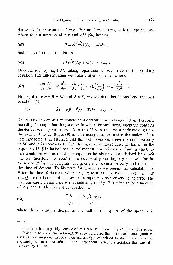
The Origins of Euler's Variational Calculus 129
derive the latter from the former. We are here dealing with the special case where Q is a function of y, x and s. 15 (58) becomes
Ldq
(60) p = e J L ~ (Lq + M ) d x ,
and the variational equation is
c Ldq
(61) eJL~T-~ff(Lq + M ) d x = c dq .
Dividing (61) by Lq + M, taking logarithms of each side of the resulting equation and differentiating we obtain, after some reductions,
d M dq d2q dL dq 2 L ( d q ~ 2 L q d 2 q (62)
dx dx M ~Sx2 + -~x q dx + \ dx ] ~ x 2 = 0 "
Noting that y = q, R = M and S = L, we see that this is precisely TAYLOR'S equation (41)
(41) I ~ - R.9 + Sy9 + 2S9p - Syy = 0 .
5.5 EULER'S theory was of course considerably more advanced than TAYLOR'S, including (among other things) cases in which the variational integrand contains the derivatives of y with respect to x. In w 27 he considered a body moving from the points A to M (Figure 9) in a resisting medium under the action of an arbitrary force. It is assumed that the body possesses a given terminal velocity at M, and it is necessary to find the curve of quickest descent. (Earlier in the paper in w 16-w 18 he had considered motion in a resisting medium in which no side condition was assumed; the equation he obtained was derived from (45) and was therefore incorrect.) In the course of presenting a partial solution he calculated P for two integrals, one giving the terminal velocity and the other the time of descent. To illustrate his procedure we present his calculation of P for the time of descent. We have (Figure 9) A P = x, P M = y, A M = s. - P and Q are the horizontal and vertical components respectively of the force. The medium exerts a resistance R that acts tangentially; R is taken to be a function of x, y and s. The integral in question is
(63) f : d x x / ( l + pp )
where the quantity v designates one half of the square of the speed, v is
15 EULER had explicitly considered this case at the end of w 22 of his i738 paper. It should be noted that although TAYLOR employed fluxions there is one significant
similarity of notation. TAYLOR used superscripts or primes to denote the values of a quantity at successive values of the independent variable, a notation that was also followed by EULER.

130 C.G. FRASER
A
P
P
9
Figure 9.
O
a function of x, y and s and is given by the equation dv = Q d x - P d y - R d s J 6
The values of L, M and V corresponding to the integrand in (63) are
(64) L - R x f l f + pp M - P x / 1 + pp V - P
2vx/v ' 2 v ~ ' x/v(1 + p p )
We have as well
(65) d V - dp p dv
(1 + p p ) ~ 2 v ~ - p p )
16 EULER did not present the derivation of the relation dv = Q d x - P d y - R d s . It may be obtained as follows. Equating forces and accelerations we have the equations
d2x dx
dt 2 - Q - dss R
a~yy= _ p a y e dt 2 ds "
Multiplying these equations by dx / d t and dy /d t respectively and summing, we obtain the desired relation.

The Origins of Euler's Variational Calculus 131
Hence the expression for P given by (58) is 17 R dx dp
~(Pdx+Qdy),/l+pp- 2Vap ( 2vdp ~ (66) P = e ,/,1 . . . . (Pdx + Qdy)x/1 + pp - ~ / .
In w 28 EULER proceeded to obtain P for a very extensive class of variational integrals. His analysis is of some interest as an indication of the range and sophistication of his theory. The variational integral is now ~oQ(~oRdx)dx, where d Q = L d s + M d y + N d x + v d p and d R = E d s + F d y + G d x + l d p . The part of this integral that will be altered is
(67) Q dx ~ R dx + Q'dx ~ R'dx + Q" dx ~ R" dx .
The changes in the terms occurring in (67) are
d. Q d x ~ R d x = V . b f i ~ R d x
d .Q'dx~R'dx = L 'qdx .b f i~R 'dx + M ' d x b f i ~ R ' d x - V'(bfi + c~/)
�9 ~ R'dx + Q 'I dx . bfl
(68) d. Q " d x f R " d x = - L"dxdq . bf i~R"dx - L ' q ' d x . c T ~ R ' d x
- M " d x . c T ~ R " d x + V" .co/~R"dx + Q"Idx .b f i
+ Q"(E'q + F' )dx 2. bfi - Q"I'dx(dfl + c~) .
Summing these expressions and equating them to zero, we obtain
(69) b f i ( - d. V ~ R d x + (L'q + M ' ) d x ~ R ' d x - L"dxdq~R"dx + Q"Idx
Hence
+ Q"(Eq + F)dx 2 - d . Q' Idx)
= c 7 ( - d. V '~R'dx + (L 'q ' + M " ) d x ~ R ' d x + Q"I 'dx)
~7 The calculation that EULER presents of P is correct, as is his corresponding calculation of this quantity for the integral that expresses the terminal speed. He suggests at the end of the solution that the equation of the problem will be obtained by taking a multiple of one of these expressions, adding it to the other and setting the result to zero. There is however a serious difficulty with this argument. The theory employed in
the calculation of P presupposes the isoperimetric condition ~o x/1 + p2 dx = constant. Hence in finding the curve of quickest descent (as this problem is formulated here) it is necessary to take into account two side conditions: one asserting that the terminal speed is given; the other that the path-length is constant. In order to handle this sort of problem it would be necessary to extend the theory to the case where there is more than one side condition present. He had considered multiple side conditions in w 38-{} 39 of his paper of 1738 and had made some progress in obtaining special results. Nevertheless he did not adapt the analysis to the case at hand, the curve of quickest descent through a resisting medium.

132 C.G. FRASER
dP (70)
P
-dd . vJ R dx + dx d(L' q + M')~R'dx - Q"(Eq + F)dx 2 + L"dx dqjR"dx + Q"dI dx + d. Q'I dx -- d. VfRdx + (L'q + M')dxSR'dx + Q"Iax - L"dxdq[R"dx -- d.Q'Idx
Integrating (70), we obtain the desired formula for P:
(71)
Q dI dx + L dx d q f R dx - Q (Eq + F) dx 2
p = e~-d.V.IRd~+(Lq+M)d~gdx+Ordx (-- d" V ~ n d x + (Lq + M ) d x ~ R d x + Qldx) .
Equation (71) encapsulates in a single general formula the numerous special results that EULER had listed in tabular form in w of his paper of 1738. ~s
5.6 To conclude our discussion of the paper of 1741 we consider another more direct way in which (59) may be generalized. Although EULER did not present the result which follows it is a very natural and straightforward extension of his theory. We simply reformulate his derivation by replacing s in Q by /7, where I I = ~ o ~ [ Q ] d x and [Q] = [Q](x, y, p). Q is now of the form Q(x , y ,p , II). We have dQ = N dx + M dy + Vdp + L d l I and d[Q] = [ N ] d x + [ m ] dy + [ V] dp + [-L] dII. We assume that ~o [Q] dx = constant holds in the
variational process. The values for the variation of 17 are
dH = 0
d/7' -- [ V ] . bfi (72)
dH" -= [V] .bfl + [ M ' ] d x . b f i + [ V ' ] . ( - c7 - bfi)
= ( [ M ' ] dx - d [ V ] ) , bfi - [ V ' ] . c7
a Because of the condition ~o [Q]dx -- constant it follows that dFl'" = d l l i ~ , . . . are zero.
We next calculate the change in ~oQdx. Because d y ' " = d y ~ . . . . . dp" = dp i~ - - . . . = dl l ' " = d/7 i~ = . . . . 0 it follows that this change
will involve only the terms Q dx, Q'dx and Q"dx. We have
dQ dx = V. b fl
(73) d Q ' d x = L ' [ V ] d x . b f l + M ' d x . b f i - V ' . b f l - V ' . c 7
18 The general difficulty discussed in the previous note arises again in connection
with EULER'S derivation of (71). He is assuming that ~o x/1 + pa dx and ~o R dx are both held constant in the variational process. However, in order to make this assumption it would be necessary to use a process in which three ordinates are varied. One way of salvaging the analysis would be to suppose that Q and R do not contain s. By calculating the value of P for ~a o R dx and combining it with (71) one would arrive at the final differential equation of the problem. The solution thus obtained would embody a result of some interest and generality.

The Origins of Euler's Variational Calculus 133
dQ"dx = - L"dx d [ V ] . bfl + L " d x Z [ M ' ] �9 bfl - L " [ V ' ]
i! q V t ! d x . c T - M d x . c y + .c 7
Summing these expressions and equating the result to zero, we obtain the equat ion
(74) ( - d V + L ' [ V ] d x + M ' d x - L " d x d [ V ] + L " d x Z [ M ' ] ) . b f l
= ( - dV ' + L " [ V ' ] d x + M " d x ) . c 7
We set A = - d V + L ' [ V ] d x + M ' d x - L " d x d [ V ] + L ' d x 2 [ M ' ] , B = - dV '
+ L " [ V ' ] d x + M " d x and calculate dP/P = (B - A)/A; (74) becomes
dP (75)
P
- d d V + L ' d x d [ V ] - L ' [ M ] d x 2 + d x d ( L ' [ V ] + M ' )
- d V + d x ( L ' [ V ] + M ' )
Let us define the variable q by means of the relation
(76) dq/dx = - [M] + d [ V ] / d x .
Integrat ing (75), we see that the expression for P given in (58) now assumes the more general form
L dx dq
(77) p = e~-dv +a~(L~V~+~) (- - d V + d x ( L [ V] + M ) ) .
Equat ion (59) in turn becomes
(78) L dx dq
eS -aV+dx(Ltvl+~t)(_ d V + d x ( L [ V ] + M ) ) = cdq .
5~7 We turn now to the subject of the isoperimetric theory as it was developed in the Methodus inveniendi. None of equations (58) to (78) or any of the accompanying analysis appear in Chapter 5 of that treatise. 19 EULER began his investigation of the isoperimetric problem there with a derivation of "EULER'S rule" for the case where there are no auxiliary variables such as /7 in the variational integrand. The case where such variables do appear is covered in
19 There is one significant piece of circumstantial evidence that EULER had explicitly considered something like the derivation of (78) when he wrote the Methodus inveniendi. In presenting the isoperimetric rule in Chapter 5 he used the notation dA for N d x - dP, where Z is the variational integrand and N = c~z/@, P = Oz/Op (p = dy/dx). On the face of it this notation seems somewhat odd, since there is no particular technical or conceptual significance for the quantity A (the integral of Ndx --dP) within the theory that is developed in Chapter 5. However, as equation (76) indicates, such a definition would emerge naturally in the course of generalizing equation (58). The notation in Chapter 5 may therefore be the vestige of a more complete isoperimetric theory that he finally decided to omit from the treatise.

134 C.G. FRASER
Proposition 5, which in the present notation is formulated as follows. Given Q = Q ( x , y , p , / 7 ) with /7=~o[Q]dx we must maximize or minimize ~oQdx subject to the condition that to[Q] dx = constant in the variational process, z~ We have as before d Q = N d x + M d y + V d p + L d / 7 and d [ Q ] = [ N ] d x + [M]dy + [V-]dp + [L]dH. The equation that is presented as solution is
(79) O = M + (a + H - ~Ldx)[M] d(V + (a + H -- SLdx)[V]) dx
where e is a constant or "multiplier". His justification of (79) was simply to extend "EuLER'S rule" by fiat to the class of problems that he had investigated in Chapter 3. Thus the equation for the free variational problem of extremaliz- ing ~oQdx is
d(V + (H - ~ Ldx)[V]) (80) 0 = M + (H - ~Ldx)[M] - dx
The variational equation for the condition ~o[Q]dx = constant is
d[V] (81) 0 = [M] dx
Using "EULER'S rule", we combine these two results and obtain (79) as the resulting equation.
Although the equation which EULZR arrived at is the correct one his demon- stration ("solutio") is spurious. The flaw in the preceding attractively simple argument is that the derivation of (80), presented in Chapter 3 of the Methodus inveniendi, is based on a one-ordinate variational process. The application of "EULER'S rule" by contrast presupposes an underlying two-ordinate variational process. In the two-ordinate process the terms which appear as coefficients of the increments no longer take the form of (80). EULER'S reasoning is both logically and mathematically unsatisfactory.
What is needed to establish Proposition 5 is a theory to handle variational integrals of the form ~oQ(x,y,p,/7)dx with /7 = ~o[Q~dx in which the side condition ~o[Q]dx = constant is present. Although he had developed precisely such a theory in his paper of 1741 he did not include it in the treatise of 1744. Let us examine how such a derivation would proceed. We begin with (78):
L dx dq (78) eS-aV+dx~LW~+M) (-- dV + dx(L[V] + M)) = cdq .
We integrate (78) and obtain - L d q
(82) i Ldx + c~ = ce f -~+M+Ltvl , x
20 We present EULER's Proposition for the case where only the first-order derivative p appears in the integrand function Z.

The Origins of Euler's Variational Calculus 135
where c~ is a constant of integration. Combin ing (78) and (82) we obtain
(83) M - dx + L [ V ] = L d x + o~ d-~
Recall f rom (76) that dq/dx = - [ M ] + d[V] /dx . Hence (83) becomes
(84) M - d~x + L [ V ] + L d x + o~ [M] dx = 0 ,
which m a y be writ ten in the form
(85) M + L d x + c ~ [ M ] - d x x + L d x + c ~ [V] = 0 .
(85) and (79) are identical, and thus the equat ion EULER obta ined in P ropo- sition 5. 21
The preceding derivat ion is a fairly natura l and direct appl icat ion of the theory that EuI~Zl~ had himself developed in his paper of 1741. His failure to include it in Chap te r 5 consti tutes a substantial weakness in the treatise and requires some comment . Fol lowing the recognit ion of the error that he had commi t ted in deriving the equat ions for the free var ia t ional p rob lem his re- search seems to have crystallized along lines that were significantly different f rom those of established research. In the course of this shift he seems to have mental ly rejected the earlier isoperimetric theory that involved integrands con- taining the pathlength as a variable. It is possible that he regarded the whole theory as mis taken or flawed because of the circumstances associated with the par t icular error that he had commit ted.
It should be noted that equat ion (79) is correct; there is as well a certain at tract ive symmet ry in the appearance in it of the multiplicative term H - SL dx. There is at times in EuI, E~'s variat ional writings (and perhaps more generally in his work in analysis 22) a tendency to derive equat ions and to
21 This derivation clearly brings to light the spurious character of EULER's demon- stration of Proposition 5. There arc two constants involved in the derivation, c and c~. c is the constant that arises in "EULER's rule"; ~ is a constant of integration that appears in the course of the derivation. If L = 0, that is, if the integrand does not contain/7, then c = ~. If however L 4= 0 then the two constants are distinct and have distinct meanings within the derivation. It is clear therefore that when L :r 0 ~ can not play the role of the constant in "EULERs rule".
a2 This tendency is apparent in EULER'S work on the summability of infinite series, discussed in [BARBEaU & LEAH, 1976]. It is also present in his research on partial differential equations of the 1730s and 1740s. DEMIDOV (1982, 329) characterises EULER'S contributions to the latter subject in the following way (p. 329): "A formal-analytical approach combined with the use of clever tricks for reducing differential equations to integrable forms; lack of any geometric interpretation either of equations or their solutions."

136 C.G. FRASER
consider their application to individual examples, with only a limited considera- tion of the character of the underlying theory.
The overall result of this situation is that the Methodus inveniendi possesses a somewhat ahistorical character in relation to earlier research in the subject. The historical meaning of the early theory was determined in the final analysis by its ultimate development and articulation, and this took place not in the 1744 treatise but in EULER'S earlier papers.
6. Overview
The early development of the calculus of variations is a story with a some- what complicated structure: different sources and authors, different methods, as well as different objects (namely variational problems differing as to the nature of the integrand and auxiliary conditions). Table 1 provides a synoptic overview of the work of the BERNOULLIS, TAYLOR and EULER. As we have seen, various notations were employed by the early authors; for purposes of comparison one standard notation has been used in Table 1.
Table 1. Synoptic overview of the early history. Note: The early researchers used several different notational systems. Throughout this table, x denotes the abscissa, y the ordinate
and s the path-length, f is the integrand function
x is the independent variable
Integrand function Comments
JAKOB BERNOULLI (1701)
TAYLOR (1715)
JOHANN BERNOULLI (1719)
General formulation of theory, but integrand functions as such do not appear.
Problem 1, f= f (y ) Problem 2, f=f(s)
Fluxional notation and techniques employed. Appearance of general integrand function.
Proposition 17, f =f(x, y, s)
General integrand functions do not explicitly appear.
Problem 1, f= f ( y ) Problem 2, f=f(s)
Isoperimetric side condition is formulated in terms of geometrical diagram. Associated equation of condition is derived analytically.
Isoperimetric side condition is formulated analytically. The associated equation of condition is derived analytically.
Isoperimetric side condition is formulated in terms of geometrical diagram. Derivaion of associated equation of condition is carried out in reference to the elements of this diagram. In Problem 5 an isochronic integral side condition is introduced.

The Origins of Euler's Variational Calculus 137
Table 1. (Contd.)
x is the independent variable
Integrand function Comments
EULER (1738)
EULER (1741)
EULER (1744)
JAKOB BERNOULLI (1_701)
f = f ( x , y)
f = g(x, y) x/1 + y,2
f = f (x, y, s) f = g(x, y, s)x/1 + y,2
f = f ( x , y, y', y") f = f ( x , y, y', y", s)
f = f (x, y, y', . . . . y("~) f = f (x , y, y', . . . . y("), 17),
dH/dx = 9(x, y, y', . . . . y("), H).
General integrand functions do not explicitly appear.
Problem 3, f = yg(s)
For the free problem: correct variational equation for f = 9(x, y) and f = 9(x, y)x/1 + y,2: incorrect equation for f = 9(x, y, s) and f = g ( x , y , s ) , / 1 + y,2.
For the isoperimetrie problem: correct variational equation for all cases.
For the free problem: correct variational equation for f = f (x , y, y', y"); incorrect equation for f = f ( x , y, y, y", s). For the isoperimetric problem: correct variational equation for all cases.
Correct variational equations derived for all cases. In Chapter 2 for the free problem with integrand f = f ( x , y, y ' , . . . , y("~).
In Chapter 3 for the free problem with integrand f = f ( x , y, y', . . . . y(")), II), where d17/dx = 9(x, y, y', . . . . y("), 17).
In Chapter 5 equations that correspond to those of Chapters 2 and 3 are derived in the ease where integral side conditions are present.
In obtaining comparison curve the path-length to each point is unaltered. A two- point variational process is employed in which both the ordinate and abscissa of each of the two varied points are altered.
(Continued)

138 C. G. FRASER
Table 1. (Contd.)
x is the independent variable
Integrand function Comments
JOHANN BERNOULLI (1719)
General integrand functions do not explicitly appear.
Problem 2 (alternate solution),
f = f(s) x/1 -- (dy/ds) 2.
Problem 3 (hanging chain), f = yg(s)
Problem 4 (brachistochrone with isoperimetric condition). f = k / ~ (x/1 -- (dy/ds) 2)
In obtaining comparison curve the path-length to each point is unatered. A two-point variational process is employed in which both the ordinate and abscissa of each of the two varied points are altered.
7. Conclusion
7.1 One conclusion that emerges fairly directly from our study concerns the relative importance of JOHANN BERNOULLI and TAYLOR in the background to EULER'S research. Established his tor iography places emphasis on the role of BERNOULLI'S paper of 1719 in the development of the subject. I t was for reasons of its alleged importance that WOODHOUSE [18101 devoted an entire chapter to it. More recently, FELLMANN & FLECKENSTEIN [1970], GOLDSTINE [1980] and FEI~ENBAUM [1985] have affirmed the value of JOHANN'S research. 23
It is clear however that the links connecting EULER'S research and TAYLOR'S were much stronger. 24 The essential analytical innovations that distinguished
23 FELLMANN 8,:: FLECKENSTEIN [1970, 53] write: "Soon after publication of Jakob's Analysis magni probIematis isoperimetrici (1701), Johann must have felt that his brother's judgement was valid, although he never said so. Only after having been stimulated by Taylor's Methodus incrementorum (1715) did he produce a precise and formally elegant solution of the isoperimetric problem along the lines of Jakob's ideas (M~moires de l'Acad6mie des sciences, 1718). The concepts set forth in this paper contain the nucleus of modern methods of the calculus of variations." GOLDSTINE [1701, 51] claims: "Jakob's 1701 paper is somewhat pedantic and tedious, but he was perhaps trying to lay the groundwork for the subject of the calculus of variations in a systematic way. In any case Johann's paper in 1718 is a more readable account of Jakob's work." FEIGENBAUM [1985, 49] suggests that the solution to the isoperimetric problem presented by JOHANN is one "considered remarkable, both then and now, for its simplicity and elegance."
24 WOODHOUSE [1810, 29 30] calls attention to TAYLOR'S equation (37) and briefly remarks on EULER'S adoption of this mode of expression, FEIGENBAUM [1985, 63] also mentions (37) and suggests that it had some importance for the later development of the

The Origins of Euler's Variational Calculus 139
EULER'S approach from the BERNOULLIS' were provided by TAYLOR. The con- siderable part of the BERNOULLIS' theory that was neglected by TAYLOR also failed to be taken up by EULER. At the level of specific technical detail there were substantial similarities in their derivation of the isoperimetric variational equations.
That an English mathematician, a member of a distinct and competing mathematical tradition, should have this importance for what is primarily a continental European development may seem surprising. It is however im- portant to appreciate the extent to which TAYLOR'S mathematical interests were defined by continental research. In a recent article FEIGENBAUM [1992] draws attention to a certain tension that existed between TAYLOR and the English mathematical establishment. She observes (p. 393), "Although the language and notation of TAYLOR'S book were Newtonian, not only did he propose what he considered to be a more sound foundation for the fluxional calculus based on finite increments, but the subject matter, physical applica- tions, and the analysis he employed were all more characteristic of continental mathematics."
7.2 Our study has also revealed some significant anomalies in the early history of the variational calculus. The first concerns the special character of a very considerable part of the BERNOULLIS' investigation. The theory associated with JAKOB'S Problem 3, reproduced and developed further by JOHANN, was not taken up by subsequent mathematicians; it became and remains today a relic from the formative years of the creation of the calculus. Another anomaly is provided by EULER'S curious decision not to include much of the isoperimetric theory of his paper of 1741 in the Methodus inveniendi. The latter was a work composed with a conspicuous absence of historical spirit. The early develop- ment of the subject did not exhibit the orderly and cumulative character that is sometimes associated with the history of the exact sciences.
7.3 The organization of the subject adopted by EULER in the Methodus inveniendi was taken over by LAORANCE when he introduced his c~-algorithm in the 1750s. LAGRANGE developed his new method exclusively in reference to the examples of Chapters 2 and 3 of EULER'S treatise. The result was that in the later eighteenth century the isoperimetric theory became somewhat mar- ginalized within variational mathematics. In his late treatise, the Lefons sur le calcul des fonctions of 1806, LAORANGE formulated the method of multipliers, a powerful theoretical tool that provided a unified approach to the various
subject. There are two reasons why a more detailed appreciation of TAYLOR'S work has not appeared in the literature. First, interest has centred primarily on continental research, especially JOHANN BERNOULLI'S paper of 1719; second, historians have tended to focus on EULER's Methodus inveniendi to the exclusion of his earlier variational writings.
140 C.G. FRASER
problems of the subject. This method forms the basis for the modern perspec- tive on the problems and techniques considered in the present paper. 2s
Acknowledgements. I am greatful to HENK Bos for comments and suggestions on a first draft of this paper. Research for the paper was financially supported by Social Sciences and Humanities Research Council of Canada grant 410920107.
References
BARBEAU, E. J., & LEAH, P. J., 1976. "Euler's 1760 paper on divergent series", tfistoria Mathematica 3, pp. 141 160.
BERNOULLI, JAKOB. 1697. "Solutio problematum fraternorum, peculiari programmate cal. Jan. 1697 Groningae, nec non Actorum Lips. mense Jun. & Dec. 1696, & Febr. 1697 propositorum: una cum propositione reciproca aliorum', in Acta eruditorum, pp. 211-217. Published in JAKOB'S Opera (1744), pp. 768-778. Reproduced in [BERNOULLI, JAKOB and JOHANN, 19911, pp. 271-282.
BERNOULLI, JAKOB. 1701. "Analysis magni problematis isoperimetrici", Acta eruditorum, pp. 213-228. Published in JAKOB'S Opera (1744),pp. 895-920, and in JOHANN'S Opera V. 2 (1742), pp. 219-234. Reproduced in [BERNOULLI, JAKOB and JOHANN, 1991].
BERNOULLI, JAKOB. 1744. Jacobi Bernoulli Basileensis opera, 2 volumes. Ed. GABRIEL CRAMER. Geneva.
BERNOULLI, JOHANN. 1719. "Remarques sur ce qu'on a donn6 jusqu'ici de solutions des Problames sur les Isoperimetres, avec une nouvelle methode courte & facile de les resoudre sans calcul, laquelle s'Gtend aussi /t d'autres probl~mes qui ont rapport /t ceux-lfi", M~moires de l'Acaddmie Royale des Sciences 1718, pp. 100-138. Repro- duced in [-BERNOULLI, JAKOB and JOHANN, 1991], pp. 527-568.
BERNOULLI, JAKOB. 1742. Johannis Bernoulli opera omnia. 4 volumes. Ed. GABRIEL CRAMER. Lausanne and Geneva.
BERNOULLI, JAKOB & BERNOULLI, JOHANN. 1991. Die Streitschriften yon Jacob und Johann Bernoulli Variationsrechnun9. Edited by H. H. GOLDSTINE with the assistance of P. RADELET-DE GRAVE. Introduction by GOLDSTINE, pp. 4-113. Published by the Naturforschenden Gesellschaft in Basel. Birkh/iuser Verlag. Basel, Boston and Berlin. This volume contains numerous selections from the Meditationes, JAKOB's scientific notebook. An early draft version of his 1701 paper will be found in Med. CCXXXIX, pp. 228-247. This selection is also reproduced by DIETZ [1959, 100-115].
Bos, H. J. M. 1974. "Differentials, higher-order differentials and the derivative in the Leibnizian calculus", Archive for History of Exact Sciences 14, pp. 1-90.
CARATHt~ODORY, C. 1952. "Einfiihrung in Eulers Arbeiten fiber Variationsrechnung", in EULER'S Opera Omnia, Ser. 1, V. 24, pp. viii-li.
DEMIDOV, S. S. 1982. "The study of partial differential equations of the first order in the 18 m and 19 th centuries", Archive for History of Exact Sciences 26, pp. 325-350.
DIETZ, P. 1959. "Die Ursprfinge der Variationsrechnung bei Jakob Bernoulli", Verhand- lungen der Naturforschenden Gesellschaft in Basel V. 70 N. 2, pp. 81-146. Contains several selections from JAKOB's Meditationes.
2s The later eighteenth-century history leading up to LAGRANGE'S theory of 1806 is described by FRASER [1992,1.

The Origins of Euler's Variational Calculus 141
EULER, L. 1726. "Constructio linearum isochronarum in medio resistente", Acta eruditorum, pp. 361-363. In the Opera omnia Ser. 2 V. 6 (1957), pp. 1-3.
EULER, L. 1736. Mechanica sire motHs scientia analytice exposita. Two volumes. Published in 1952 (ed. P. ST~CKEL) as volumes 1 and 2 of series 2 of EULER'S Opera omnia.
EU~ER, L. 1738. "Problematis isoperimetrici in latissimo sensu accepti solutio generalis", in Commentarii academiae scientiarum Petropolitanae 6 (1732/3), pp. 123-155. Re- printed in EULER'S Opera omnia Ser. 1, V. 25 (1952),pp. 13-40.
EULER, L. 1740. "De linea celerrimi descensus in medio quocunque resistente", Commen- tarii academiae scientiarum Petropolitanae 7 (1734/35), pp. 135-139. Reprinted in Opera omnia Ser. 1, V. 25 (1952), pp. 41-53.
EULER, L. 1741. "Curvature maximi minimive proprietate gaudentium inventio nova et facilis", in Commentarii academiae scientiarum Petropolitanae 8 (1736), 159-190. Re- printed in Opera omnia Set. 1, V. 25 (1952), pp. 54-80.
EULER, L. 1744. Methodus inveniendi curvas lineas maximi minimive proprietate 9audentes sire solution problematis isoperimetrici latissimo sensu accepti, Lausanne. Reprinted as Opera omnia Ser. 1, V. 24 (1952).
FEIGENBAUM, L. 1985. "Brook Taylor and the method of increments", Archive for History of Exact Sciences 34, pp. 1-140.
FEIGENBAUM, L. 1992. "The fragmentation of the European mathematical community", in The investigation of difficult things: essays on Newton and the history of the exact sciences in honour of D. T. Whiteside, pp. 383-397. Cambridge University Press.
FELLMANN, E. A., & FLECKENSTEIN, J. O. 1970. "Bernoulli, Johann (Jean) I", in Dictionary of scientific biography, ed. C. C. GILLISPIE, V. 2, pp. 51-55.
FRASER, C. 1985. "J. L. Lagrange's changing approach to the foundations of the calculus of variations", Archive for History of Exact Sciences 32, pp. 151-191.
FRASER, C. 1991. Review of [-BERNOULLI, JAKOB and JOHANN, 1991], in Centaurus 34, pp. 367 369.
FRASER, C. 1992. "Isoperimetric problems in the variational calculus of Euler and Lagrange', Historia Mathematica 19, pp. 4-23.
GOLDSTINE, H. H. 1980. A history of the calculus of variations from the 17 th through the 19 th century. Springer-Verlag.
GOLDSTINE, H. H. 1991. Introduction to [-BERNOULLI, JAKOB and JOHANN, 1991], pp. 1-113.
HERMANN, J. 1729. "Theoria generalis motuum qui nascuntur a potentiis quibusvis in corpora indesinenter agentibus, sive haec corpora in vacuo ferantur sive in medio resistenti." Commentarii academiae scientiarum imperiaIis PetropoIitanae 2 (1727), pp. 139-173.
TAYLOR, B. 1715. Methodus incrementorum directa & inversa. London. WOODHOUSE, R. 1810. A treatise on isoperimetrical problems and the calculus of vari-
ations. Cambridge.
Institute for the History and Philosophy of Science and Technology
Victoria College University of Toronto
(Received October 28, 1993)