the origin of the 1500-year climate cycles in holocene...

Clim. Past, 3, 569–575, 2007www.clim-past.net/3/569/2007/© Author(s) 2007. This work is licensedunder a Creative Commons License.

Climateof the Past

The origin of the 1500-year climate cycles in HoloceneNorth-Atlantic records

M. Debret1, V. Bout-Roumazeilles2, F. Grousset3, M. Desmet4, J. F. McManus5, N. Massei6, D. Sebag6, J.-R. Petit1,Y. Copard6, and A. Trentesaux2

1Laboratoire de Glaciologie et de Geophysique de l’Environnement, UMR CNRS 5183, BP96, 38402, St Martin d’Heres,France2PBDS Laboratoire, UMR 8110 CNRS, Universite de Lille 1, 59 655 Villeneuve d’Ascq, France3EPOC, UMR CNRS 5805, Universite de Bordeaux I, Avenue des Facultes, 33405 Talence, France4EDYTEM Laboratoire, UMR 5204, Universite de Savoie, CISM, Campus Scientifique 73376 Le Bourget du Lac Cedex,France5Woods Hole Oceanographic Institution, Woods Hole, MA 02543, USA6Laboratoire de Morphodynamique Continentale et Cotiere, UMR CNRS 6143, Departement de Geologie, Universite ofRouen, 76821 Mont-Saint-Aignan Cedex, France

Received: 21 December 2006 – Published in Clim. Past Discuss.: 26 March 2007Revised: 20 July 2007 – Accepted: 18 September 2007 – Published: 1 October 2007

Abstract. Since the first suggestion of 1500-year cyclesin the advance and retreat of glaciers (Denton and Karlen,1973), many studies have uncovered evidence of repeatedclimate oscillations of 2500, 1500, and 1000 years. Duringlast glacial period, natural climate cycles of 1500 years ap-pear to be persistent (Bond and Lotti, 1995) and remarkablyregular (Mayewski et al., 1997; Rahmstorf, 2003), yet theorigin of this pacing during the Holocene remains a mystery(Rahmstorf, 2003), making it one of the outstanding puzzlesof climate variability. Solar variability is often consideredlikely to be responsible for such cyclicities, but the evidencefor solar forcing is difficult to evaluate within available dataseries due to the shortcomings of conventional time-seriesanalyses. However, the wavelets analysis method is appro-priate when considering non-stationary variability. Here weshow by the use of wavelets analysis that it is possible todistinguish solar forcing of 1000- and 2500- year oscilla-tions from oceanic forcing of 1500-year cycles. Using thismethod, the relative contribution of solar-related and ocean-related climate influences can be distinguished throughoutthe 10 000 yr Holocene intervals since the last ice age. Theseresults reveal that the 1500-year climate cycles are linkedwith the oceanic circulation and not with variations in so-lar output as previously argued (Bond et al., 2001). In thislight, previously studied marine sediment (Bianchi and Mc-Cave, 1999; Chapman and Shackleton, 2000; Giraudeau et

Correspondence to:M. Debret([email protected])

al., 2000), ice core (O’Brien et al., 1995; Vonmoos et al.,2006) and dust records (Jackson et al., 2005) can be seento contain the evidence of combined forcing mechanisms,whose relative influences varied during the course of theHolocene. Circum-Atlantic climate records cannot be ex-plained exclusively by solar forcing, but require changes inocean circulation, as suggested previously (Broecker et al.,2001; McManus et al., 1999).

1 Introduction

It was suggested, for both the late Glacial and the Holocene,a 1500 yr variability of the climate (Bond et al., 1995, 1997,2001). Initially associated with the so-called Dansgaard-Oeschger oscillations (Dansgaard et al., 1993), this pe-riod seems to occur independently of the general glacial-interglacial climate changes. According to these results, themillennial-scale variability was attributed to the same forc-ing, ruling out any direct link with the ice-sheet oscilla-tions. In North Atlantic as in other part of the world, manypaleo-climatic records of the last 10 000 years show a patternof rapid climate oscillations with cyclicity around 1–2 kyrs.Since the pioneering studies of Gerard Bond on IRD fromthe North Atlantic Ocean (Bond et al., 1995, 1997, 2001),the 1500-year cycle during the Holocene was tentatively at-tributed to solar activity (Bond et al., 2001), to ocean cur-rent intensity variation (Bianchi and McCave, 1999), to tidal

Published by Copernicus Publications on behalf of the European Geosciences Union.

570 M. Debret et al.: Origin of 1500-year cycles in Holocene North-Atlantic records

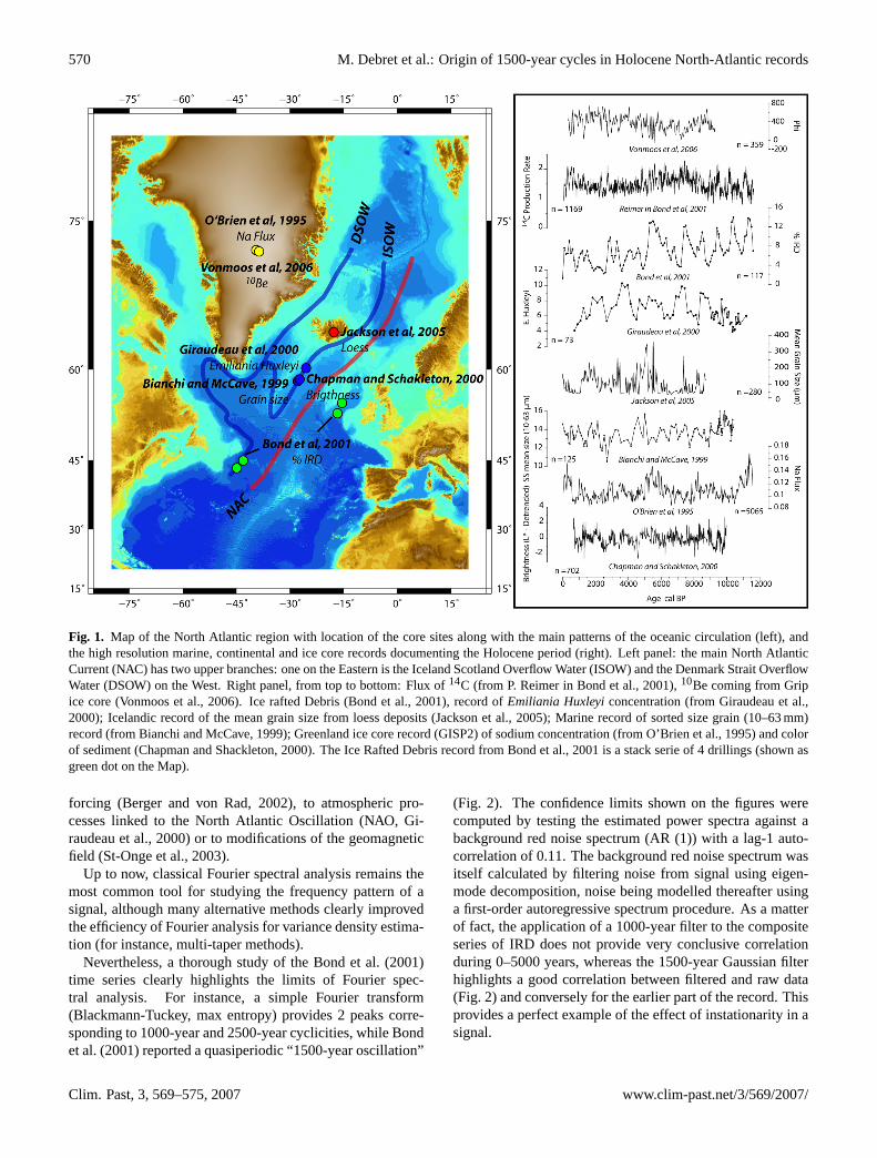
Fig. 1. Map of the North Atlantic region with location of the core sites along with the main patterns of the oceanic circulation (left), andthe high resolution marine, continental and ice core records documenting the Holocene period (right). Left panel: the main North AtlanticCurrent (NAC) has two upper branches: one on the Eastern is the Iceland Scotland Overflow Water (ISOW) and the Denmark Strait OverflowWater (DSOW) on the West. Right panel, from top to bottom: Flux of14C (from P. Reimer in Bond et al., 2001),10Be coming from Gripice core (Vonmoos et al., 2006). Ice rafted Debris (Bond et al., 2001), record ofEmiliania Huxleyiconcentration (from Giraudeau et al.,2000); Icelandic record of the mean grain size from loess deposits (Jackson et al., 2005); Marine record of sorted size grain (10–63 mm)record (from Bianchi and McCave, 1999); Greenland ice core record (GISP2) of sodium concentration (from O’Brien et al., 1995) and colorof sediment (Chapman and Shackleton, 2000). The Ice Rafted Debris record from Bond et al., 2001 is a stack serie of 4 drillings (shown asgreen dot on the Map).

forcing (Berger and von Rad, 2002), to atmospheric pro-cesses linked to the North Atlantic Oscillation (NAO, Gi-raudeau et al., 2000) or to modifications of the geomagneticfield (St-Onge et al., 2003).

Up to now, classical Fourier spectral analysis remains themost common tool for studying the frequency pattern of asignal, although many alternative methods clearly improvedthe efficiency of Fourier analysis for variance density estima-tion (for instance, multi-taper methods).

Nevertheless, a thorough study of the Bond et al. (2001)time series clearly highlights the limits of Fourier spec-tral analysis. For instance, a simple Fourier transform(Blackmann-Tuckey, max entropy) provides 2 peaks corre-sponding to 1000-year and 2500-year cyclicities, while Bondet al. (2001) reported a quasiperiodic “1500-year oscillation”

(Fig. 2). The confidence limits shown on the figures werecomputed by testing the estimated power spectra against abackground red noise spectrum (AR (1)) with a lag-1 auto-correlation of 0.11. The background red noise spectrum wasitself calculated by filtering noise from signal using eigen-mode decomposition, noise being modelled thereafter usinga first-order autoregressive spectrum procedure. As a matterof fact, the application of a 1000-year filter to the compositeseries of IRD does not provide very conclusive correlationduring 0–5000 years, whereas the 1500-year Gaussian filterhighlights a good correlation between filtered and raw data(Fig. 2) and conversely for the earlier part of the record. Thisprovides a perfect example of the effect of instationarity in asignal.

Clim. Past, 3, 569–575, 2007 www.clim-past.net/3/569/2007/

M. Debret et al.: Origin of 1500-year cycles in Holocene North-Atlantic records 571

Fig. 2. Spectral analysis and filtered component of the stacked record from Bond et al. (2001). FFT highlights 2 major peaks in accordancewith Blackmann-Tuckey and Maximum Entropie (left panel top). A small peak with a low energy around 1450-year appear only in FFT,however this periodicity is present between 1000 and 6000 years BP as shown by Gaussian filter applied on the series. On the other hand,the early Holocene period clearly displays 1000 years cycles. The bandwidth is 200 years for the Gaussian filters; we used e.g. 900–1100years and 1400–1600 years, respectively.

This result demonstrates the limited ability of classicalFourier spectral analysis to detect a 1500-year fluctuationthat evolves through time. Such observations are typicalof non-stationary processes, in which frequency content andstatistical properties change through time. Wavelet analysis(WA) presents the advantage of describing non-stationarities,i.e. discontinuities, changes in frequency or magnitude (Tor-rence and Compo, 1998). Redundancy of the continuouswavelet transform is used to produce a time/frequency ortime/scale mapping of power distribution, called the localwavelet spectrum (or scalogram). As a major advantage withrespect to classical Fourier analysis, the local wavelet spec-trum allows direct visualization of the changing statisticalproperties in stochastic processes with time.

WA performed on Bond et al. (2001) time series highlights2 major cyclicities (up to 90% of confidence): 1000 and 2500years (Fig. 3). The 2500-year cycle is continuous throughoutthe Holocene whereas the 1000-year cycle is absent duringthe Late Holocene (until 5000 years). This time-slice is char-acterized by an increase in spectral power at another periodaround 1500 years, reaching its maximum intensity at 3000years but remains with a low confidence (<50%). Bond etal. (2001) had compared their records with the14C produc-

tion rate (Reimer in Bond et al., 2001) to justify the solar in-fluence. We have processed the14C production rate (Reimerin Bond et al., 2001) and solar modulation function inferredfrom the 10Be (Vonmoos et al., 2006) following the sameprotocol as the one used when processing the IRD data. WAreveals the same general feature for the14C production rate,10Be and IRD for the dominant periodicities with specialemphasis on the attenuation of the 1000-year cycle during5000–0 years period (Fig. 3). For the last millennia the prob-lem is difficult to disentangle because only one cycle is con-cerned with a probable reappearance of 1000-yr cycle. Thisis likely in accordance with Little Ice Age well recognizedin North Atlantic Area. These results corroborate the solarorigin of the cycles at 1000 and 2500 years recorded in theIRD series. Nevertheless the two series show some discrep-ancies: a 1600-year cycle is recorded during the Holocene inthe14C production rate excepted during 5000–0 years whenthe 1500-year cycle of Bond’series is expressed (but with alow level of significance). Thus the occurrence of this 1500-year cycle in the IRD series records a forcing other than solaractivity. Is it a pacing induced by a combination of cyclicitiesor a problem of proxy sensitivity to an other forcing factor?

www.clim-past.net/3/569/2007/ Clim. Past, 3, 569–575, 2007


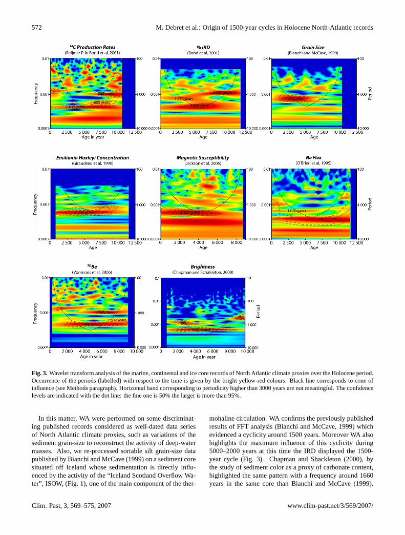
Fig. 3. Wavelet transform analysis of the marine, continental and ice core records of North Atlantic climate proxies over the Holocene period.Occurrence of the periods (labelled) with respect to the time is given by the bright yellow-red colours. Black line corresponds to cone ofinfluence (see Methods paragraph). Horizontal band corresponding to periodicity higher than 3000 years are not meaningful. The confidencelevels are indicated with the dot line: the fine one is 50% the larger is more than 95%.

In this matter, WA were performed on some discriminat-ing published records considered as well-dated data seriesof North Atlantic climate proxies, such as variations of thesediment grain-size to reconstruct the activity of deep-watermasses. Also, we re-processed sortable silt grain-size datapublished by Bianchi and McCave (1999) on a sediment coresituated off Iceland whose sedimentation is directly influ-enced by the activity of the “Iceland Scotland Overflow Wa-ter”, ISOW, (Fig. 1), one of the main component of the ther-

mohaline circulation. WA confirms the previously publishedresults of FFT analysis (Bianchi and McCave, 1999) whichevidenced a cyclicity around 1500 years. Moreover WA alsohighlights the maximum influence of this cyclicity during5000–2000 years at this time the IRD displayed the 1500-year cycle (Fig. 3). Chapman and Shackleton (2000), bythe study of sediment color as a proxy of carbonate content,highlighted the same pattern with a frequency around 1660years in the same core than Bianchi and McCave (1999).



This is also confirmed with a 1700-years cycle in theEmilia-nia Huxleyiconcentration record, a proxy of surface hydrol-ogy, in a core off Iceland (Giraudeau et al., 2005).

So we can propose that the IRD are not good proxies totrack thermohaline activity in North Atlantic area. Indeedthe oceanic forcing (1500 years) is found but only with avery low significance in the signal unlike solar forcing. Also,we can postulate that the IRD series, classically used as areference of the climatic fluctuations during the Holocene,records at least one dominant forcing: solar activity for wave-lengths at 1000- and 2500-year (up to 90% of the signal), andone minor: oceanic activity for the cyclicity at 1500 yearscharacterising the late Holocene. According to the actualstate of the art, this “double” forcing on the IRD signal canbe mainly explained by the respective influence of solar ac-tivity on continental ice-sheets or calving, during the EarlyHolocene, and, for a lower level, of oceanic currents inten-sity strength on the geographical distribution of IRD in theNorth Atlantic Ocean during 5000–0 years cal BP. A ques-tion remains: what are the processes allowing to link solarcycle and IRD deposit in north Atlantic area? The dynamicof the ice sheet could be involved but implies a time responselag that is difficult to identificate. Perhaps could the sea iceand/or calving processes be a good contributor of this patternhowever it remains still unclear.

In addition to analysis of several marine paleoclimaticproxies, the detailed Holocene variations of both ice-coreand continental parameters were studied. The GISP 2 icecore from the summit of Greenland (Fig. 1) provides a pre-cise and accurately-dated record of climatic changes duringthe Holocene. We looked at the evolution of sodium con-centration in the ice because it is thought to represent thedirect deposition of sea spray (O’Brien et al., 1995). WAof this signal reveals an unexpected result (Fig. 3): the vari-ations of sodium shows an “oceanic forcing”-like cyclicityat 1600 years (1500–1700) during the late Holocene withmaximum of intensity during the 5000–0 years cal BP. Thestriking feature of sodium flux in ice likely reflecting the cy-clonic activity forced by ocean activity could be explainedby considering the ocean-atmosphere coupling. Indeed inthe North Atlantic Ocean the meridional overturning circu-lation obviously has a direct influence on sea-ice repartitionsubsequently affecting the synoptic atmospheric configura-tion in the North Atlantic area (O’Brien et al., 1995). As aresult, the variations of the oceanic circulation near Icelandduring the Holocene as recorded both by grain-size evolu-tion (Bianchi and McCave, 1999) and Calcareous nannofos-sils abundance (Giraudeau et al., 2000) modify indirectly theatmospheric transfer of oceanic Na toward Greenland. How-ever the very low confidence of this frequency with the sig-nal of sodium flux in Greenland shows that an other proxy isneeded. In order to constrain the atmospheric variability dur-ing the Holocene, a loess series from Iceland (Fig. 1, Jacksonet al., 2005), the only dust record available, was analysed us-ing WA. The results display a dominant 1700 years variabil-

Figure 4: Lomb periodogram of initial data (bold line) FFT of cubic spline interpolated data

Acknowledgements:

Special thanks and respects to the memory of G. Bond: his innovative paper inspired this255

work.

We wish to thank Matthew Jackson, Delia Oppo, Jacques Giraudeau, Vincent Peyaud,

Emmanuel Chapron, Paula J. Reimer, Juerg Beer for their valuable insight, avaibility and/or for

having shared their data. The friendly review of Nick McCave, Pascal Yiou, Dominique Raynaud

and Anne deVernal has been essential. We are very grateful to Annette Witt and the anonymous260

reviewer for very constructive criticisms and Luc Beaufort, Natascha Otto, Denis-Didier

Rousseau for their help during the review processing. This work is supported by ANR project:

Intégration des contraintes Paléoclimatiques pour réduire les Incertitudes sur l’évolution du

Climat pendant les périodes Chaudes- PICC (ANR-05-BLAN-0312-02).

265

Fig. 4. Lomb periodogram of initial data (bold line) FFT of cubicspline interpolated data.

ity (Fig. 3) evidencing the influence of ocean activity on theoverlying low-altitude atmospheric configuration confirmingthe oceanic pacing felt in Greenland ice core. The ratherdispersive values obtained for the “so-called 1500-year cy-cle” through WA on the various data series analysed couldresult from discrepancies in their respective model-age (iso-topic stratigraphy, AMS14C, ice-core tuned).

2 Conclusion

By re-visiting well-known series from the North AtlanticOcean, wavelet analysis reveals that the Holocene millen-nial variability is composed of at least three periodicities.Our results strongly suggest that two wavelengths are di-rectly forced by solar activity (1000 and 2500-year cycles)whereas the third one (1600-year cycle, dominant during5000–0 years) may correspond to oceanic internal forcing.Our results, based on a purely mathematical approach arenot able to provide any additional explanation on the ori-gin(s) of this oceanic variability, which may result from at-mospheric water transport (Broecker et al., 2001) or a persis-tent internal salt oscillator (McManus et al., 1999) or perhapsan orbital modulation of the mechanisms driving millennial-and centennial-scale climatic change through the Holoceneas suggest by Turney et al. (2005). They nevertheless ruleout the strictly external climate forcing due to variations insolar output through a linear process.

Although cyclicities of 1000 years and 2500 years areapparently broadly distributed over the whole climatic sys-tem (Nederbragt and Thurow, 2005) the global extension ofthe 1600-year cycle is much more controversial. Indeed the1500-year cycle is often evidenced within various series onthe basis of a simple comparison with the mis-interpretedIRD reference dataseries, thus introducing a systematic biasin their conclusions. When submitted to our WA, these series



display in fact cyclicities of 2500 and 1000 years instead ofthe expected 1500-year one. The circum-North Atlantic cli-mate is particularly sensitive to changes in oceanic forcingdue to changes in the strength of the meridional overturningcirculation (Manabe and Stouffer, 2000; Alley et al., 1997;McManus et al., 2004). It remains to be seen whether thisoceanic forcing extends globally, but the approach presentedhere provide a means to evaluate the respective influence ofsolar and oceanic forcing in high-resolution records from ap-propriate locations throughout the climatic system.

3 Methods

3.1 Wavelet transforms

The wavelet transform, contrary to the Fourier transform, isused to decompose a signal into a sum of small wave func-tions of a finite length that are highly localized in time, fordifferent exploratory scales. By difference, Fourier trans-form aims to separate a signal into infinite-length oscillatoryfunctions (sine waves) like, which results in a complete lossof time information as separated frequencies always applyto the entire length of the signal. Hence, instationary pro-cesses can not be described correctly using infinite complexexponentials, because of changes in frequency content acrosstime. Wavelet transform is a band-pass filter which consistsof convoluting the signal with scaled and translated formsof a highly time-localized wave function (the filter), the so-called “mother wavelet”. The reference waveletψ , referredto as the “mother wavelet”, comprises two parameters fortime-frequency exploration, i.e. a scale parameter (a) and atime-localization parameter (b) so that:

ψa,b(t) =1

√a

· ψ

(t − b

a

)(1)

Parametera produces “daughter wavelets” for investigationat different scale levels, while parameterb allows translationof each daughter wavelet across time to detect changes infrequency content. The continuous wavelet transform of asignals(t), producing the wavelet spectrum, is defined as:

S(a, b) =

+∞∫−∞

s(t) ·1

√a

· ψ

(t − b

a

)· dt (2)

Time-frequency representation actually plots the waveletpower the time series. In practice, since the wavelet trans-form consists in applying a low-pass filter to a given timeseries, wavelet power is computed by fast Fourier transform(FFT), which makes easier the convolution of the time seriesby the wavelet filter (convolution in the time domain cor-responds to a simple algebric product in the frequency do-main). Once the Fourier transforms of the time series and the

wavelet filter have been computed, the inverse Fourier trans-form of their product is calculated as follows:

Wn(s) =

N−1∑k=0

xk·ψ∗(s.ωk)e

iωknδt (3)

with N: number of points in the time series,s: scale of daugh-ter wavelets,n: time index,k: frequency index,xk: Fouriertransform of the initial time seriesxn, ψ∗: complex conju-gate of the Fourier transform ofψ (wavelet filter),ω : fre-quency,δt: time step. Finally, the wavelet power of the com-plex functionWn(s) is defined as the square of the amplitudeof the wavelet transform, that is,|Wn(s)|

2. The resulting plotof the wavelet power spectrum|Wn(s)|

2 is a contour mapin which frequency, Fourier period or wavelet scale (y-axis),and power (z-axis) are plotted against time (x-axis). Sev-eral types of wavelet are available. In this study the Mor-let wavelet (a gaussian-modulated sine wave) was chosen forcontinuous wavelet transform:

ψ(η) = π−1/4· eimη · e−η

2/2 (4)

where η is a dimensionless time parameter and m is thewavenumber that defines the basic resolution of the motherwavelet. A wavenumber of 10 was used, this choice offeringa good trade-off between frequency and temporal resolutionfor the time series analyzed herein.

3.2 Cone of influence

To avoid edge effects and spectral leakage that are producedby the finit length of the time series, all series were zero-padded to twice the data length. However, zero-paddingcauses the lowest frequencies near the edges of the spectrumto be underestimated as more zeros enter the series. The areadelineating this region is known as the cone of influence andmarks those parts of the spectrum where energy bands arelikely to be less powerful than they actually are because edgeeffects are becoming important.

3.3 Statistical test

For all local wavelet spectra, monte carlo simulation wasused to assess the statistical significance of peaks. Back-ground noise for each signal was estimated and separatedusing singular spectrum analysis. Autoregressive modellingwas then used for each noise time series to determine theAR(1) stochastic process against which the initial time serieswas to be tested. AR(1) background noise could be eitherwhite (AR(1)=0) or red noise (AR(1)>0).

3.4 Unevenly time sampled records

Blanks/gaps in the data were filled up/interpolated using acubic spline interpolant (passes exactly through each datapoint). Although we did not use the weighted wavelet Z-transform algorithm, the cubic spline interpolation we used



for handling unevenly-spaced data would not imply signif-icant changes in the results of spectral/continuous waveletanalysis: for instance as shown in Fig. 4, a Lomb peri-odogram performed on the initial data of the most hetero-geneously sampled series leads to the same results as a FFTof the interpolated time series (here interpolated to 4 timesthe length of the initial series).

Acknowledgements.Special thanks and respects to the memory ofG. Bond: his innovative paper inspired this work.

We wish to thank M. Jackson, D. Oppo, J. Giraudeau, V. Peyaud,E. Chapron, M. Magny, P. J. Reimer, J. Beer for their valuableinsight, avaibility and/or for having shared their data. The friendlyreview of N. McCave, P. Yiou, D. Raynaud and A. deVernal hasbeen essential. We are very grateful to A. Witt and the anonymousreviewer for very constructive criticisms and L. Beaufort, N. Otto,D.-D. Rousseau for their help during the review processing. Thiswork is supported by ANR project: “Integration des contraintesPaleoclimatiques pour reduire les Incertitudes sur l’evolution duClimat pendant les periodes Chaudes”- PICC (ANR-05-BLAN-0312-02).

Edited by: L. Beaufort

References

Alley, R. B., Mayewski, P. A., Sower, T., Stuiver, M., Taylor, K.C., and Clark, P. U.: Holocene climate instability: a prominent,widespread event 8200 yrs ago, Geology, 25, 483–486, 1997.

Berger, W. H. and von Rad, U.: Decadal to millennial cyclicity invarves and turbidites from the Arabian Sea: Hypothesis of tidalorigin, Global Planet. Change, 34, 313–325, 2002.

Bianchi, G. G. and McCave, N.: Holocene periodicity in North At-lantic climate and deep-ocean flow south of Iceland, Nature, 397,515–517, 1999.

Bond, G. G., Kromer, B., Beer, J., Muscheler, R., Evans, M., Show-ers, W., Hoffmann, S., Lotti-Bond, R., Hajdas, I., and Bonani,G.: Persistent Solar Influence on North Atlantic Climate Duringthe Holocene, Science, 294, 2130–2136, 2001.

Bond, G., Showers, W., Cheseby, M., Lotti, R., Alsami, P., deMeno-cal, P., Priore, P., Cullen, H., Hajdas, I., and Bonani, G.: A per-vasive millennial-scale cycle in North Atlantic Holocene glacialclimates, Science, 278, 1257–1266, 1997.

Bond, G. and Lotti, R.: Iceberg discharges into the north Atlanticon millennial time scales during the last glaciation, Science, 267,1005–1010, 1995.

Broecker, W., Sutherland, S., and Peng T.-H.: A possible 20th-century slowdown of Southern ocean deep Water formation, Sci-ence, 286, 1132–1135, 2001.

Chapman, M. R. and Shackleton, N.: Evidence of 550-year and1500-year cyclicities in North Atlantic circulation pattern duringthe Holocene, The Holocene, 10(3), 287–291, 2000.

Dansgaard, W., Johnsen, S. J., Clausen, H. B., Dahl-Jensen, D.,Gundestrup, N. S., Hammer, C. U., Hvidberg, C. S., Steffensen,J. P., Sveinbjornsdottir, A. E., Jouzel, J., and Bond, G.: Evidencefor general instability of past climate from a 250-kyr ice-corerecord, Nature, 364, 218–220, 1993.

Denton, G. H. and Karlen, W.: Holocene climatic variations – Theirpattern and possible cause, Quat. Res., 3, 155–205, 1973.

Giraudeau, J., Cremer, M., Manthe, S., Labeyrie, L., and Bond, G.:Coccolith evidence for instabilities in surface circulation southof Iceland during Holocene times, Earth Planet. Sci. Lett., 179,257–268, 2000.

Jackson, M. G., Oskarson, N, Trønnes, R. G., McManus, J.F., Oppo, D., Gronveld, K., Hart, S. R., and Sachs, J. P.:Holocene loess deposition in Iceland: Evidence for millennial-scale atmosphere-ocean coupling in the North-Atlantic, Geology,33, 509–512, 2005.

Manabe, S. and Stouffer, R. J.: Study of abrupt climate change by acoupled ocean-atmosphere model, Quat. Sci. Rev., 19, 285–299,2000.

Mayewski, P. A., Meeker, L. D., Twickler, M. S., Whitlow, S., Yang,Q., Lyons, W. B., and Prentice, M.: Major features and forcing ofhigh latitude nothern hemisphere atmospheric circulation using110 000-year long glaciochemical series, J. Geophys. Res., 102,26 345–26 366, 1997.

McManus, J. F., Francois, R., Gherardi, J.-M., Keigwin, L. D.,and Brown-Leger, S.: Collapse and rapid resumption of Atlanticmeridional circulation linked to deglacial climate changes, Na-ture, 428, 834–837, 2004.

McManus, J. F., Oppo, W. D., and Cullen, J. L.: A 0.5-million-year record of millennial-scale climate variability in the NorthAtlantic, Science, 283, 971–974, 1999.

Nederbragt, A. J. and Thurow, J.: Geographic coherence ofmillennial-scale climate cycles during the Holocene, Pal3, 221,313–324, 2005.

O’Brien, S. R., Mayewski, P. A., Meeker, L. D., Meese, D. A.,Twickler, M. S., and Whitlow, S. L.: Complexity of Holoceneclimate as reconstructed from a Greenland ice core, Science, 270,1962–1964, 1995.

Rahmstorf, S.: Timing of abrupt climate change: a precise clock,Geophys. Res. Lett., 30, 1510, doi:10.1029/1003GL017115,2003.

Saint-Onge, G., Stoner, J. S., and Hillaire-Marcel, C.: Holocene pa-leomagnetic records from St. Lawrence Estuary, eastern Canada:Centennial- to millenial-scale geomagnetic modulation of cos-mogenic isotopes, Earth Planet. Sci. Lett., 209, 113–130, 2003.

Stuiver, M., Reimer, P. J., Bard, E., Beck, J. W., Burr, G. S., Hughen,K. A., Kromer, B., McCormac, F. G., van der Plicht, J., andSpurk, M.: INTCAL98 radiocarbone age calibration, Radiocar-bon, 40, 1041–1083, 1998.

Torrence, C. and Compo, G. P.: A practical guide to wavelet analy-sis, Bull. Am. Meteorol. Soc., 79, 61–78, 1998.

Turney, C., Baillie, M., Clemens, S., Brown, D., Palmer, J., Pilcher,J., Reimer, P., and Leuschner, H. H.: Testing solar forcing ofpervasive Holocene climate cycles, J. Quat. Sci., 20, 511–518,2005.

Vonmoos, M., Beer, J., and Muscheler, R.: Large varia-tions in Holocene solar activity – constraints from10Bein the GRIP ice core, J. Geophys. Res., 111, A10105,doi:10.1029/2005JA011500, 2006.


the origin of the 1500-year climate cycles in holocene...

Documents