THE OPTIMIZATION OF DATA COMPRESSION ALGORITHMS

By

WANG-REI TANGMaster of Engineering in Civil and Environmental Engineering

Massachusetts Institute of TechnologyJune 1999

Submitted to the Department of Civil & Environmental EngineeringIn Partial Fulfillment of the Requirement for the Degree of

ENGINEER'S DEGREEIN CIVIL AND ENVIROMENTAL ENGINEERING

At the

MASSACHUSETTS INSTITUTE OF TECHNOLOGYSeptember 2000

@ 2000 Wang-Rei TangAll rights reserved.

The author hereby grants to MIT permission to reproduce and to distribute publicly paperand electronic copies of this thesis for the purpose of other works

Signature of AuthorDeartment of ffivil and Environmental Engineering

August 4, 2000

Certified by

Accepted by

Professor Jerome ConnorAssociate Professor, Civil and Environmental Engineering

Thesis Supervisor

I.-,

Professor Daniele VenezianoChairman, Department Committee on Graduate Studies

MASSACHUSETTS INST!ITUTEOF TECHNOLOGY

SFP 1 5 2000

I-IRRARIES

BARKER

THE OPTIMIZATION OF DATA COMPRESSION ALGORITHMS

By

WANG-REI TANG

Submitted to the Department of Civil & Environmental EngineeringIn Partial Fulfillment of the Requirement for the Degree of

Engineer's DegreeIn Civil & Environmental EngineeringMassachusetts Institute of Technology

Abstract

Data compression is used to reduce the number of bits required to store or transmitinformation. A data compression algorithm is a set of rules or procedures for solvingdata compression problems in a finite number of steps. The efficient of a algorithm isimportant since it is directly related to cost and time.

Data compression algorithms can be categorized according to the techniques used to dothe compression. Statistical methods use variable-size codes, with the shorter codesassigned to symbols that appear more often in the data, and longer codes assigned tosymbols that appear less often in the data. Shannon-Fano encoding, the Huffman code,and arithmetic coding are all in the statistical method family.

This thesis presents an overview of the different data compression algorithms, theirdevelopment and the improvements from one technique to another. The code forHuffman algorithm is developed at the end of the thesis.

Thesis Supervisor: Jerome ConnorTitle: Professor of Civil and Environmental Engineering

Acknowledgements

First of all, I would like to thank my advisor, Professor Jerome Connor, for all his help

during the entire year, for his understanding and trust in everything that I was doing.

I also want to give very special thanks to my parents and brother for their continuous

support for whatever decision I made. Another big thank-you goes to my relatives and

friends for their support through all these years.

Finally, I thank God for all the wonderful things that happened to me.

3

TABLE OF CONTENTS

TA BLE O F FIG U R ES.................................................................................................................................. 5

CH A PTER O N E IN TR O D U CTIO N ......................................................................................................... 6

CHAPTER TWO BASICS OF DATA COMPRESSION ........................................................................ 9

2.1 BRIEF HISTORY OF DATA COM PRESSION........................................................................................ 9

2.2 LOSSLESS AND LOSSY COMPRESSION ......................................................................................... 10

2.3 SYM M ETRICAL AND ASYM M ETRIC COM PRESSION ...................................................................... 11

2.4 SYM BOLIC DATA COM PRESSION................................................................................................... 11

2.5 BRAILLE CODE..........................................................................................................- - .. --------........ 12

CHAPTER THREE RUN-LENGTH ENCODING................................................................................14

3.1 INTRODUCTION ..................................................................................................- -. ----------............ 14

3.2 O PERATION..........................................................................................................--------------.......... 143.3 CONSIDERATIONS ..................................................................................................... ------.............. 18

CHAPTER FOUR STATISTICAL CODING......................................................................................... 20

4.1 INTRODUCTION .....................................................................................................-- ........ . . 204.2 M ORSE CODE ..................................................................................................................--.-.-.-...... 20

4.3 INFORM ATION THEORY .............................................................................................. ....... 214.4 V ARIABLE-SIZE CODES ......................................................................................................... 25

CHAPTER FIVE SHANNON-FANO CODING..................................................................................... 28

5.1 INTRODUCTION ............................................................................................................ . ---.-.. --...... 285.2 O PERATION .......................................................................................................... . ....... 28

5.3 CONSIDERATIONS...................................................................................................- ... -----.......... 31

CH A PTER SIX H U FFM A N C O D IN G ................................................................................................. 33

6.1 INTRODUCTION ............................................................................................................ --.......... 336.2 O PERATION............................................................................................. .............................. 33

6.3 CONSIDERATIONS ................................................................................................ ...... .............. 35

CHAPTER SEVEN ARITHMETIC CODING....................................................................................... 40

7.1 INTRODUCTION .....................................................................................- -....... ---.. ................... 407.2 O PERATION .................................................................................. ... ........---.--.-.--........................ 417.3 CONSIDERATIONS ........................................................................................................--.-.......... 45

CH A PTER EIG H T H U FFM A N C O D E ................................................................................................. 47

CH PA TER N IN E C O N CLU SIO N ........................................................................................................... 58

A PPEND IX A.............................................................................................................................................. 61

R EFER EN C ES .................................................................................................................--------..----.-........ 65

4

Table 2.1

Figure 3.1

Figure 3.2

Figure 4.1

Figure 4.2

Figure 4.3

Table 5.1

Table 5.2

Table 5.3

Table 5.4

Table 5.5

Table 6.1

Table 6.2

Table 6.3

Table 7.1

Table 7.2

5

TABLE OF FIGURES

Symbolic data encoding

Flow chart for run-length compression

Flow chart for run-length decompression

Morse code

Fixed-size code

Variable-size code

An example of character set probability occurrence

Initial process for Shannon-Fano compression

Completed process for Shannon-Fano compression

Another version of completed Shannon-Fano process

Perfect splits for Shannon-Fano process

Huffman code

Huffman code

Huffman code for symbols with equal probability

The process of Arithmetic encoding

The process of Arithmetic decoding

INTRODUCTION

Data compression may sound like one of those technical phrases that only

computer programmers can understand or need to understand. In fact, data compression

is present in many aspects of our daily life. For example, when a boy wants to send a

message to a girl, instead of sending the message "I love you", he might use "IVU". In

such a case, since the message was sent by three symbols instead of ten, it can be called

data compression.

Another example of a data compression application that we see every day is a fax

machine. Exchanging faxes is one of the most common tasks of many businesses. As we

all know, sending a fax is faster and more efficient than regular mail. But fax devices

would not work without data compression algorithms. The image of the document is not

being sent over the phone line as it is. A fax machine compresses the data before it is

sent. Data compression helps to reduce the time needed to transmit the document. The

cost of transmission is reduced 10 or more times.

So what is data compression? Data compression is the process of converting an

input data stream into another data stream that has a smaller size. A stream is either a file

or a buffer in memory. The basic idea of data compression is to reduce the redundancy.

That is why a compressed file cannot be compressed again since a compressed file should

have a little or no redundancy.

Why is data compression important? The answer to this question is data

compression saves a lot of time and money. First of all, people like to accumulate data

6

CHAPTER ONE

but hate to throw it away. No matter how big the storage device is, sooner or later it is

going to overflow. Data compression is useful because it delays the overflow. Secondly,

people often don't have the time to wait online, thus they don't like to wait for a long

time for downloads. When doing a transaction on the Internet or downloading music or

file, even a few seconds can make us feel it is a long time to wait. Data compression is to

find innovative ways to represent information using as few bits as possible for storage

and transmission. Most of the time, saving time means saving money.

In the past, documents were stored on paper and kept in filing cabinets. It was

very inefficient in terms of storage space and also the time taken to locate and retrieve

information when required. Storing and accessing documents electronically through

computers have replaced this traditional way of storage.

In digital systems, there are three reasons to use data compression: storage

efficiency, transmission bandwidth conservation, and transmission time reduction. The

capacity of a storage device can be effectively increased with methods that compress a

body of data on its way to a storage device and decompresses it when it is needed.

Compressing data at the sending end and decompressing data at the receiving end can

effectively increase the bandwidth of a digital communication link. Lastly, with data

compression techniques, many files can be combined into one compressed document,

making transferring data through the Internet easier.

Data compression is achieved by reducing redundancy, but this also makes the

data less reliable. Adding check bits and parity bits, a process that increases the size of

the codes, increases the redundancy, thus does make the data more reliable. Data

reliability is a more recent field while data compression existed even before the advent of

7

computer. In this thesis, some of the basic concepts of data compression are introduced.

In the later chapters, different data compression algorithms for symbolic data are

analyzed. We will go through not only the technique used in each algorithm but also the

advantages and disadvantages of each algorithm are experienced.

8

CHAPTER TWO BASICS OF DATA COMPRESSION

2.1 Brief history of data compression

The need to efficiently represent information has been with us since man learned

how to write. The art of writing in shorthand can be traced back to the first century B.C.

when a form of shorthand was used to record the speeches of the Roman orator Cicero.

Shorthand is a system that uses simple abbreviations, or symbols to represent letters of

the alphabet, words or phrases. This is a form of data compression in writing.

Two important events occurred in the 1800s. In 1829, the invention of Braille

code by Louis Braille created a system of writing for blind people. Braille codes

represent the letters of the alphabet by combinations of raised and flat dots. These dots

can be read by touch of fingers. Later in 1843, S.F.B. Morse developed an efficient code

consisting of dots, dashes and spaces to allow transmitting messages electrically by

telegraph. It assigns short easy codes to E, I, and other frequently transmitted letters, and

longer codes to Q, Z, and other infrequently occurring letters. The general law of data

compression is then developed, to assign short codes to common events and long codes to

rare events. There are many ways to implement this law, and an analysis of any

compression method will show that deep inside it works by obeying this general law.

More recently, in the late 1940's were the early years of Information Theory. The

idea of entropy and redundancy was starting to be introduces. The first well-known

method for compressing digital signals was the Shannon-Fano method. Shannon and

Fano developed this algorithm that assigns binary bits to unique symbols that appear

9

within a given data file. While the Shannon-Fano was a great development, it has

quickly superseded by a more efficient coding system, the Huffman algorithm.

Huffman coding is very similar to Shannon-Fano coding. The difference is that

Huffman coding is a bottom-up technique while Shannon-Fano coding uses a top-down

technique for building the binary tree. Huffman coding has become the best known and

widely used statistical coding technique to result from the studies of information theory

and probability.

In the last fifteen years, Huffman coding has been replaced by arithmetic coding.

Arithmetic coding is more complex than any other coding. It replaces a stream of input

symbols with a single floating-point number.

Dictionary-based compression algorithms use a completely different method to

compress data. The main idea of dictionary compression is to eliminate the redundancy

of storing repetitive strings for words and phrases repeated within a text stream.

Dictionary compression replaces an entire string of symbols by a single token. This

approach is extremely effective for compressing text where strings of characters

representing words occur frequently. LZ77 and LZ78 have been developed as dictionary

compression. LZ77 is also called a sliding window technique.

2.2 Lossless and lossy compression

Data compression techniques can be divided into two major families: lossless and

lossy. Lossless compression can recover the exact original data after compression. It is

used mainly for compressing database records, spreadsheets or word processing files,

10

where exact replication of the original is essential. For example, text files containing

computer programs may become worthless if even one bit gets modified.

Lossy compression will result in a certain loss of accuracy in exchange for a

substantial increase in compression. Lossy compression is more effective when used to

compress graphic images and digitized voice. If the loss of data is small, we may not be

able to tell the difference.

2.3 Symmetrical and asymmetric compression

Symmetrical compression is the case where the compressor and decompressor use

basically the same algorithm but work in different directions. In general, symmetrical

compression is used where the file is compressed as often as decompressed.

Asymmetrical compression is used when either the compressor or decompressor

works much harder. In environments where files are updated all the time and backups are

made, compressor executes a simple algorithm and the decompressor executes a slow and

complex algorithm. The opposite case is where files are decompressed and used very

often. Then a simple decompression algorithm and a complex compression algorithm

will be operated.

2.4 Symbolic data compression

As shown in Table 2.1, data compression algorithms implement these length

changes as fixed-to-variable, variable-to-fixed, or, by combining both, variable-to-

variable-length encoding. Run-length coding and the front-end models of Lempel-Ziv

11

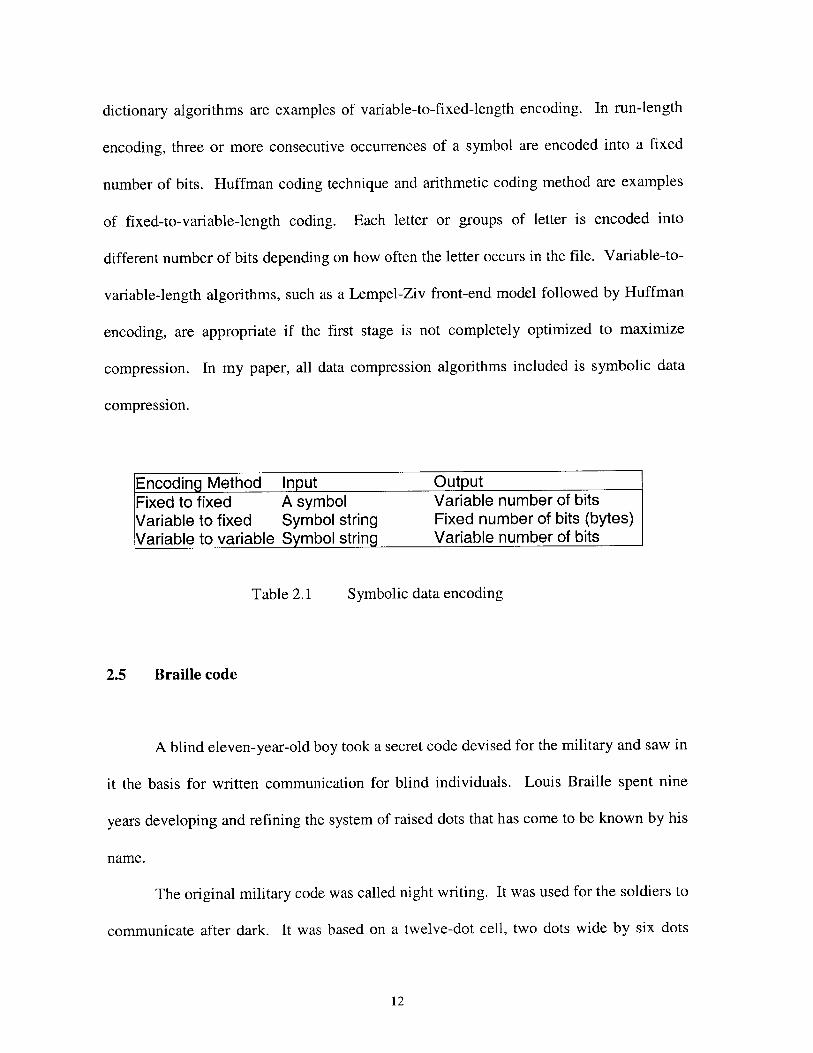
dictionary algorithms are examples of variable-to-fixed-length encoding. In run-length

encoding, three or more consecutive occurrences of a symbol are encoded into a fixed

number of bits. Huffman coding technique and arithmetic coding method are examples

of fixed-to-variable-length coding. Each letter or groups of letter is encoded into

different number of bits depending on how often the letter occurs in the file. Variable-to-

variable-length algorithms, such as a Lempel-Ziv front-end model followed by Huffman

encoding, are appropriate if the first stage is not completely optimized to maximize

compression. In my paper, all data compression algorithms included is symbolic data

compression.

Encoding Method Input OutputFixed to fixed A symbol Variable number of bitsVariable to fixed Symbol string Fixed number of bits (bytes)Variable to variable Symbol string Variable number of bits

Table 2.1 Symbolic data encoding

2.5 Braille code

A blind eleven-year-old boy took a secret code devised for the military and saw in

it the basis for written communication for blind individuals. Louis Braille spent nine

years developing and refining the system of raised dots that has come to be known by his

name.

The original military code was called night writing. It was used for the soldiers to

communicate after dark. It was based on a twelve-dot cell, two dots wide by six dots

12

high. Each of the 12 dots can be flat or raised. Each dot or combination of dots within

the cell represents a letter or phonetic sound. The problem with the military code was

that human fingertip couldn't feel all the dots at one touch.

Louis Braille created a six-dot cell, two dots wide by three dots high. The

information content of a group is equivalent to 6 bits, resulting in 64 possible groups. In

fact, letters don't require all 64 codes, the remaining groups are used to code digits,

punctuations and common words such as and, for and of and common strings of letters

such as "ound," "ation," and "th."

The amount of compression achieved by Braille may seem small but books in

Braille tend to be very large. Imagine that if the books get old and dots become flat, a lot

of reading errors will appear. The basic concept in Braille Code is to use fixed code

length for different letters, digits and symbols. It is similar to the Run-Length encoding

which assigns fixed length code to symbols when they have three or more consecutive

occurrences.

13

RUN-LENGTH ENCODING

3.1 Introduction

Run-length coding is one of the simplest data compression algorithms. The idea

behind this approach to data compression simply represents the principle of encoding

data: If a data item d occurs n consecutive times in the input stream, then the n

occurrences would be replaced with the single pair nd. The repeating data item d is

called a run. The run length of n is the consecutive occurrences of the data item d. For

example, "bbbb" will be "4b". We also need to add a control symbol before "4b". For

example, "abbbb4b" will be "a@4b4b" instead of "a4b4b". If a control symbol is not

added, computer does not know if "4b" is "4b" or "bbbb",when decompressed the data.

In this case, @ is used as a control symbol.

3.2 Operation

As mentioned in the introduction, a run-length coder replaces sequences of

consecutive identical data items with three elements: a control symbol, a run-length count

and a data item. A control symbol is used to tell the computer that the compression

should start from here. Let's see a simple example. Given "hippppp899999w", it can be

compressed as "hi @ 5p8 @59w". Fourteen characters were used to represent the original

message. After the compression, only 10 characters are needed. We used @ as the

14

CHAPTER THREE

control symbol. It tells the computer to take the first character right after this symbol as

the number of repetition of a data item. That data item is the character right after the

count. Let's see another example. Given "happy555", it can be compressed as

ha@2py@35. The compression expands the original string rather than compresses it,

since two consecutive letters was compressed to three characters. This is not an

optimized compression.

It takes at least three characters to represent any number of consecutive identical

letters. We should have it in mind that only three or more repetitions of the same

character will be replaced with a repetition factor. Figure 3.1 is a flow chart for such a

simple run-length text compressor.

After reading the first character, the character count is 1 and the character is

saved. Each of the following characters is read and compared to the saved character. If

they are identical to the saved character, the repeat count will be incremented by 1. If

they are not identical to the saved character, the next operation will depend on the

number of the repeat count. If the repeat count is less than 3, the saved character will be

written on the compression file for a number of times. The newly read character will be

saved and the repeat count goes back to zero. If the repeat count is equal or greater than

3, an "@" is written, followed by the repeat count plus one and by the saved character.

Figure 3.2 is the decompression flow chart. The program starts with the

compression flag off. The flag is used to determine whether the decompressor should

read the next character as a character from the original message or as a repeat count of

the followed character. If an "@" is read, the flag is turned on immediately and is turned

off after generating a certain character for repeat count plus one time.

15

Char. count C:=ORepeat count R:=O

Figure 3.1 flow chart for run-length compression.

16

Figure 3.2 Flow chart for run-length decompression

17

I

3.3 Considerations

1.

As mentioned previously, run-length coding is highly effective when there are a

lot of runs of consecutive symbols. In plain English text there are not many repetitions.

There are many "doubles" but a "triple" is rare.

2.

In the basic encoding flow chart illustrated in Figure 3.1, it was assumed that the

repeat count was capable of having an unlimited range of values. In reality, the

maximum value that the repeat count can contain depends on the function of the character

code level employed. For an 8-level (eight bit per character) character code, the

maximum value of the repeat count is 255. However, we can extend 255 to 258 by using

a small trick. Since a repeat count of 1, 2 or 3 is only helping in counting, we can set

repeat count 0 instead of 3. When writing out to the decompression file, repeat count 8

would be 5 in this case. This method is not very helpful since only a value of 3 is

extended. But one can always add additional repeat count comparison to test for the

maximum value permitted to be stored in the character count.

3.

The character "@" was used as a control symbol in our examples. A different

control symbol must be chosen if "@"may be part of the text in the input stream.

18

Choosing a right control symbol can be tricky. Sometimes the input stream may contain

every possible character in the alphabet. The MNP5 method provides a solution.

MNP stands for Microcom Networking Protocol. The MNP class 5 method is

commonly used for data compression by modems. It has a similar flow chart as run-

length coding. When three or more identical consecutive characters are found in the

input stream, the compressor writes three copies of the character on the output stream

followed by a repeat count. When the decompressor reads three identical consecutive

characters, it knows that the next character will be a repeat count. For example,

"abbbcdddd" will be compressed as "abbbOcdddl". A disadvantage of this method is that

when compressing three identical consecutive characters, writing four characters to the

output stream instead of the original three characters is inefficient. When compressing

four identical consecutive characters, there is no compression. The compression only

really works when there are more than four characters.

19

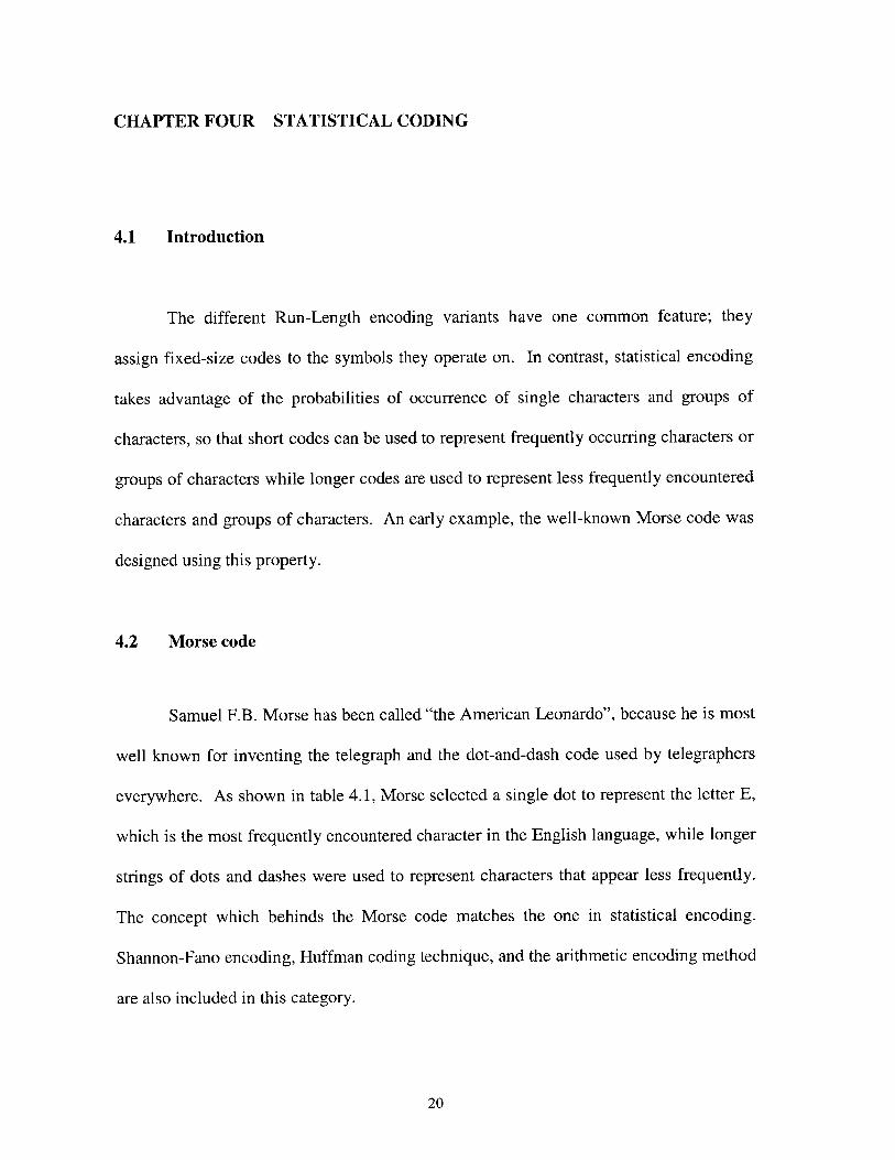
CHAPTER FOUR STATISTICAL CODING

4.1 Introduction

The different Run-Length encoding variants have one common feature; they

assign fixed-size codes to the symbols they operate on. In contrast, statistical encoding

takes advantage of the probabilities of occurrence of single characters and groups of

characters, so that short codes can be used to represent frequently occurring characters or

groups of characters while longer codes are used to represent less frequently encountered

characters and groups of characters. An early example, the well-known Morse code was

designed using this property.

4.2 Morse code

Samuel F.B. Morse has been called "the American Leonardo", because he is most

well known for inventing the telegraph and the dot-and-dash code used by telegraphers

everywhere. As shown in table 4.1, Morse selected a single dot to represent the letter E,

which is the most frequently encountered character in the English language, while longer

strings of dots and dashes were used to represent characters that appear less frequently.

The concept which behinds the Morse code matches the one in statistical encoding.

Shannon-Fano encoding, Huffman coding technique, and the arithmetic encoding method

are also included in this category.

20

A .- N -. 1 .--- PeriodB -... 0 --- 2..-- Comma --C -.-. P .-. 3 ...- ColonCh --- Q --.- 4 ....- Questionmark ....

D -.. R .-. 5 .,... Apostrophe ---.E . S ... 6 -.... HyphenF ..-. T - 7--... DashG -. U ..- 8 --.. Parentheses

H .... V ...- 9 ---. QuotationmarksI .. W .- 0 ----J .-- xK -.- YL .-.. ZM

Figure 4.1 Morse code

4.3 Information theory

In 1948, Claude Shannon from Bell Labs published "The Mathematical Theory of

Communication" in the Bell System Technical Journal, along with Warren Weaver. This

surprising document is the basis for what we now call information theory, a field that has

made all modem electronic communications possible. Claude Shannon isn't well known

to the public at large, but his "Information Theory" makes him at least as important as

Einstein. The important concepts from information theory lead to a definition of

redundancy, so that later we can clearly see and calculate how redundancy is reduced, or

eliminated, by the different methods.

Information theory is used to quantify information. It turns all information into

the on-or-off bits that flip through our computers, phone, TV sets, microwave ovens or

21

anything else with a chip in it. So what is information? Information is what you don't

know. If I tell you something that you already know, I haven't given you any

information. If I tell you something that surprise you, then I have given you some

information. We're used to thinking about information as facts, data, and evidence, but

in "Information Theory", information is uncertainty. When Shannon started out, his

simple goal was just to find a way to clear up noisy telephone connections. The

immediate benefit of information theory is that it gives engineers the math tools needed

to figure out channel capacity, how much information can go from A to B without errors.

The information we want is the "signal," not the "noise".

As mentioned earlier, information is uncertainty. For example, when we toss a

coin, the result of any toss is initially uncertain. We have to actually throw the coin in

order to resolve the uncertainty. The result of the toss can be head or tail, yes or no. A

bit, 0 or 1 can express the result. A single bit resolves the uncertainty in the toss of a

coin. Many problems in real life can be resolved, and their solutions expressed by means

of several bits. Finding the minimum number of bits to get an answer to a question is

important. Assume that we have 32 cards; each number between 1 and 32 is assigned on

one card. None of the cards have the same number. If I want to draw a card, what is the

minimum number of yes/no questions that are necessary? We should divide 32 into two,

and start by asking, "is the result between 1 and 16?" If the answer is yes, then the result

should be in range 1 and 16. This range should then be divided into two. The process

continues until the range is reduced to a single number, the final answer.

We know now it takes exactly five questions to get the result. This is because 5 is

the number of times 32 can be divided in half. Mathematically 5 = log32 , that's why the

22

logarithm is the mathematical function that expresses information. Another approach to

the same problem is to ask the question "given a non-negative integer N, how many digits

does it take to express it?" Of course the answer depends on N, but it also depends on

how we want it to be presented. For decimal digits, base 10 is used; for binary ones

(bits), base 2 is used. The number of decimal digits required to represent N is

approximately log N. The number of binary digits required to represent N is

approximately logN

Let's see another example. Given a decimal (base 10) number with k digits, how

much information is included in this k-digit number? We can find out the answer by

calculating how many bits it takes to express the same number. The largest number can

be expressed by k-digit decimal number is 10 ' -1. Assuming it takes x bits to express

the same number. The largest number can be expressed by x-digit binary number is

2' -1. Since 10k -l= 2' -1,thenwe get

log2

If we select base 2 for the logarithm, x = k logyo ~3.22k. This shows that one decimal

digit equals that contained in about 3.22 bits. In general, to express the fact that the

information included in one base-n digit equals that included in log" bits, we can use

x= klog".

Let's think about the transmitter. It is a piece of hardware that can transmit data

over a communications line, such as a channel. It sends binary data. In order to get

general results, we assume that the data is a string made up of occurrences of the n

symbols a, through a,. Think about a set that has n-symbol alphabet. We can think of

23

each symbol as a base-n digit, which means that it is equivalent to log" bits. The

transmitter must be able to transmit at n discrete levels.

Assume that the speed of the transmission is s symbols per time unit. In one time

unit, the transmitter can send s symbols, which is equal to s log" bits. We use H to

represent the amount of information transmitted each time unit, H = s log" . Let's

express H in terms of the probabilities of occurrence of the n symbols. We assume that

symbol a, occurs in the data with probability P. In general, each symbol has a different

probability. Since symbol a, occurs P percent of the time in the data, it occurs on the

average sfi times each unit, so its contribution to H is - s1i log 2 F . The sum of the

contributions of all n symbols to H is thus H = - s i"1 log 2 Pi

Since H is the amount of information, in bits, sent by the transmitter in one time

unit, and it takes time 1/s to transmit one symbol, so the amount of information contained

in one base-n symbol is thus H/s. This quantity is called the entropy of the data being

transmitted. We can define the entropy of a single symbol ai as -P log21 P. This is the

smallest number of bits needed, on the average, to represent the symbol.

As we can see from the formula, the entropy of a symbol depends on the

individual probability P. It becomes the smallest when all n probabilities are equal.

This can be used to define the redundancy R in the data. The redundancy is the

difference between the entropy and the smallest entropy.

R= -j1log 2 1 +log"

24

When yP log 2 P = log", there is no redundancy. The concept of entropy will be used

in the later chapter as well. It is very important and is used in many fields, not just in

data compression.

4.4 Variable-Size codes

As mentioned earlier, statistical encoding tends to use short codes to represent

frequently occurring characters and groups of characters while longer codes are used to

represent less frequently encountered characters and groups of characters. Why is it

important to use variable-size codes? We will use the following cases to show how

variable-size codes reduce redundancy.

Given four symbols X 1, X2 , X 3 , and X4. In the first case, all symbols appear in

our file with equal probability, 0.25. The entropy of the data is -4(0.25 log20.25) = 2

bits/symbol. Two is the smallest number of bits needed, on the average, to represent each

symbol. Table 4.2 shows four 2-bit codes 00, 01, 10 and 11 are assigned to the symbols.

Symbol Probability CodeX1 0.25 00X2 0.25 01X3 0.25 10X4 0.25 11

Table 4.2 Fixed-size code

Let's look at another case where all symbols appear in the file with different

probabilities. As shown in Table 4.3, X1 appears most frequently, almost half of the time.

25

X2 and X3 appear as often as a quarter of the time, and X4 appears only one percent of the

time. The entropy of the data is -(0.49 log20.49 + 0.25 log20.25 + 0.25 log20.25 +0.01

log20.01) = 1.57 bits/symbol. Thus 1.57 is the smallest number of bits needed, on

average, to represent each symbol. If we still assign four 2-bit codes as in case one, it

may not be efficient since four 2-bits codes produce the redundancy R = -1.57 +

(4*2*0.25) = 0.43 bits/symbol.

Symbol Probability Code A Code B

X1 0.49 1 1

X2 0.25 01 01X3 0.25 001 010

X4 0.01 000 101

Table 4.3 Variable-size code

If we assign our symbols with variable-size as Code A in Table 4.3, the average

size is 1*0.49 + 2*0.25 + 3 * 0.25 + 3*0.01 = 1.77 bits/symbol. Then the redundancy

will be -1.57 + 1.77 = 0.2 bits/symbol, which is less than the case when four 2-bits size

codes were used. This fact is suggesting variable-size code.

Variable-size codes have two important properties. One of them was mentioned

above, short codes represent more frequently occurred symbols while long codes

represent less frequently occurred symbols; the other is the prefix property. Given a 10-

symbol string X2X3X1X4X4X1 X2X3X3X2. All symbols occur with similar frequency. We

can encode this string with Code A as the follows:

01001100000010100100101

26

It takes 23 bits. Using 23 bits to encode 10 symbols makes an average size of 2.3

bits/symbol. To get a close result to the best, we need to use an input stream with at least

thousand of symbols. That result will be really close to the calculated average size, 1.77

bits/symbol.

We should be able to decode the binary string with the code A given in Table 4.3.

However, encoding the 10-symbol string with code B result in difficulty in the decoding

process. Let's encode the 10-symbol string with code B as follows:

01010110110110101001001

It takes 23 bits just like code A. How about decoding? When the decompressor starts

decoding from the first bit, it knows the symbol will be either X2 or X3 . But after taking

one or two more bits, it doesn't know how to decode. The above binary string can

decode as starting with X2X3... or X3X4 .... The reason that it works with code A but

not code B is that code A has a prefix property that code B doesn't have. Prefix property

makes sure that the code for each symbol is not a prefix for other symbol. For example,

if the bit for X2 is assigned as 01, then the bits for any symbol cannot be assigned starting

with 01. This is why in code A, X3 and X4 have to start with 00, which is different from

01 of X2.

27

CHAPTER FIVE SHANNON-FANO CODING

5.1 Introduction

The first well-known method for effective variable-size coding is now known as

Shannon-Fano coding. Claude Shannon at Bell Labs and R. M. Fano at M.I.T. developed

this method nearly simultaneously. The basic idea is in creating code words with

variable code length, like in the case of Huffman codes, which was developed few years

later. Shannon-Fano coding has a lot in common with Huffman coding.

As mentioned earlier, Shannon-Fano coding is based on variable length code

words. Each symbol or group of symbols has a different length code depending on the

probability of its appearance in a file. Codes for symbols with low probabilities have

more bits, and codes for symbols with high probabilities have fewer bits, though the

codes are of different bit lengths, they can be uniquely decoded. Arranging the codes as a

binary tree solves the problem of decoding these variable-length codes.

5.2 Operation

1. For a given list of characters, get the frequency count of each character.

2. Sort the list of characters according to their frequency counts. The characters

are arranged in descending order of their frequency count.

28

3. Divide the list into two subsets that have the same or almost the same total

probability.

4. The first subset of the list is assigned to digit 1, and the second subset is

assigned to digit 0. This means that the codes for the characters in the first

part will all start with 1, and the codes in the second part will all start with 0.

5. Repeat step 3 and 4 for each of the two parts, subdividing groups, and adding

bits to the codes until no more subset exist.

Character ProbabilityX1 0.05X2 0.05X3 0.35X4 0.30X5 0.10X6 0.05X 7 0.10

Table 5.1 An example of character set probability occurrence.

First, the characters are sorted in descending order. Then the list forms two

subsets. In our subset construction process, we will group the characters into each subset

so that the probability of occurrence of the characters in each subset is equal or as nearly

equal as possible. In this example, the first subset contains X3 and X4, and the second

subset contains the rest of the list. The total probability is 0.65 for the first subset, and

0.35 for the second subset. The two symbols in the first subset are assigned codes that

start with 1, while other symbols in the second subset are assigned codes that start with 0.

29

Note that after the initial process, as shown in Table 5.2, X3 and X4 in the first subset

isn't unique. Thus, a 1 and 0 must be added to the pairs. The same process should be

followed by the second subset. The second subset is divided into two subsets. Then the

same process we did earlier is repeated. A completed Shannon-Fano coding process is

shown in Table 5.3.

Character ProbabilityX3 0.35 1

X4 0.30 1

X5 0.10 0

X7 0.10 0Xi 0.05 0X2 0.05 0X6 0.05 0

Table 5.2 Initial process for Shannon-Fano compression

Character ProbabilityX3 0.35 1 1

X4 0.30 1 0X5 0.10 0 1 1X7 0.10 0 1 0X1 0.05 0 0 1

X2 0.05 0 0 0 1X6 0.05 0 0 0 0

Table 5.3 Completed process for Shannon-Fano compression

30

The average size of this code is 0.35 * 2 + 0.30 * 2 + 0.10 * 3 + 0.10 * 3 + 0.05 *

3 + 0.05 * 4 + 0.05 * 4 = 2.45 bits/symbol. The entropy, which is the smallest number of

bits needed on average to represent each symbol, is

-(0.35 log20.35 +0.30 log20.30 +0.10 log20.10 +0.10 log20.10 +0.05 log20.05

+0.05 log20.05 +0.05 log20.05) ~ 2.22.

5.3 Considerations

One of the problems associated with the development of the Shannon-Fano code

is the fact that the procedure to develop the code can be changeable. It is important

where we make a split in the subset construction process. Let's repeat the previous

example but divide the list between X5 and X7. In this case, the first subset contains X3 ,

X4 and X5 and the second subset contains all of the rest of the list. The total probability is

0.75 for the first subset and 0.25 for the second subset. Table 5.4 illustrates the new

version of the completed Shannon-Fano process.

Character ProbabilityX3 0.35 1 1X4 0.30 1 0 1

X5 0.10 1 0 0X7 0.10 0 1Xi 0.05 0 0 1

X2 0.05 0 0 0 1X6 0.05 0 0 0 0

Table 5.4 Another version of the completed Shannon-Fano process

31

The average size of the code is 0.35 * 2 + 0.30 * 3 + 0.10 * 3 + 0.10 * 2 + 0.05 *

3 + 0.05 * 4 + 0.05 * 4 = 2.65 bits/symbol. The reason the code of Table 5.4 has a longer

average size is that the splits were not as good as those of Table 5.3. Shannon-Fano

coding produces better codes when the splits are better. The optimal split is when the

two subsets in every split have very close total probability. The perfect splits produce the

best codes. So what is the perfect split? If the two subsets of every split have the same

total probability, the perfect case is introduced. Table 5.5 illustrates this case.

The entropy of this code is 2.5 bits/symbol. The average size of the code is 0.25 *

2 + 0.25 * 2 + 0.125 * 3 + 0.125 * 3 + 0.125 * 3 + 0.125 * 3 = 2.5 bits/symbol. It is

identical to the entropy. This indicates that it is the theoretical minimum average size,

with zero redundancy. We can conclude that the Shannon-Fano coding gives the best

result when the symbols have probabilities of occurrence that are negative powers of 2.

Character ProbabilityX3 0.25 1 1

X4 0.25 1 0X5 0.125 0 1 1

X7 0.125 0 1 0X1 0.125 0 0 1X2 0.125 0 0 0

Table 5.5 Perfect splits for Shannon-Fano process

32

HUFFMAN CODING

6.1 Introduction

Huffman coding appeared first in the term paper of a M.I.T. graduate student,

David Huffman, in 1952. Since then, it has become the subject of intensive research into

data compression. Huffman coding is the major data compression technique applicable

to text files. Even though it was introduced forty-eight years ago, Huffman coding is still

extremely popular and used in nearly every application that involves the compression and

transmission of digital data, such as fax machines, modems, computer networks, and high

definition television.

Huffman coding shares most characteristics of Shannon-Fano coding. Symbols

with higher probabilities get shorter codes. Huffman Coding also has the unique prefix

property and produces the best codes when the probabilities of the symbols are negative

powers of 2. However, building the Huffman decoding tree is done using a completely

different algorithm from that of the Shannon-Fano method. The Shannon-Fano tree is

built from the top down (leftmost to the rightmost bits), and the Huffman tree is built

from the bottom up (right to left).

6.2 Operation

Huffman coding assigns the optimal unambiguous encoding to the symbols. We

need to construct a binary tree to perform Huffman compression. This is done by

33

CHAPTER SIX

arranging the symbols of the alphabets in a descending order of probability. Then the

process involves repeatedly adding the two lowest probabilities and resorting. This

process continues until the sum of the probabilities of the last two symbols is 1. Once

this process is complete, a Huffman binary tree can be generated. The last symbol, which

was formed with the sum of the total probability 1, is the root of the binary tree.

Let's use the example in Table 6.1 to go through the steps of the algorithm. For

the given list of five character and sorted frequency counts:

1. X4 and X5 are combined to form X45, and the probability of the new symbol is

simply the sum of the probability of X4 and X5 , 0.2. Now sort the list.

2. With four symbols left in the list with probabilities of 0.4, 0.2, 0.2, and 0.2,

we arbitrary select X45 and X3. The new symbol X345 has the probability of

0.4. Sort the list.

3. With three symbols left in the list with probabilities of 0.4, 0.4 and 0.2, we

arbitrary select X2 and X345. The new symbol X2345 has the probability of 0.6.

4. Finally, we combine the remaining two symbols, X1 and X345. The last

combined symbol is X1 2 3 45 with the probability of 1.

The tree is now completed. In order to make a binary tree, we should assign bit 0 or 1 to

each edge of the tree. Starting with adding bit 1 to the root, we arbitrary add bit 1 to the

top edge, and bit 0 to the bottom edge, of every pair of edges.

As we can see from this example, the least frequent two symbols were X4 and X5.

They were combined into X45. This shows that adding bit 1 to codes which is assigned to

34

X4 5 will give the code of X4 and by adding bit 0 will give the code of X5 . The same

concept applies to all other combined symbols and their child nodes.

Character

X1

X 2

X 3

X 4

X 5

Probability

10.4

0.2

0.2

0.1

0.1

Table 6.1 Huffman code

6.3 Considerations

1.

When several symbols have the same frequency of occurrence, we may be able to

develop two or more sets of codes to represent the Huffman coding. This kind of

situation presents us with an interesting problem on deciding which code to use. To

illustrate how this problem occurs, we use our previous example from Table 6.1.

At step 2 of the previous example, we arbitrary select X45 and X3 out of X2, X3

and X45. If we had selected X2 and X3, the code set might be changed as shown in Table

6.2.

35

Character

X1 0.4 1X145 1

X2 0.2 1 0.6 X12345

X23 0

X3 0.2 0 0.4

X4 0.1 1

X45 0X5 0.1 0 0.2

Table 6.2 Huffman code

The average size of the first code is 0.4*1 + 0.2*2 + 0.2*3 + 0.1*4 + 0.1*4 = 2.2

bits/symbol. The average size of the second code is 0.4*2 + 0.2*2 + 0.2 * 2 + 0.1* 3 +

0.1*3 = 2.2 bits/symbol, just the same as the previous one.

It turns out that arbitrary decisions made when constructing the Huffman tree

affect the individual codes but not the average size of the codes. Although over a long

period of time the use of either code should produce the same result in terms of efficiency

expressed as the sum of encoded bits, in actuality, a more appropriate choice is to select

the code whose average length varies the least. That is, the code whose variance is the

smallest of all. The variance of the first code is:

0.4(1-2.2)2 + 0.2(2-2.2)2+ 0.2(3-2.2) 2+ 0.1(4-2.2) 2+ 0.1(4-2.2) 2 = 1.36.

The variance of the Huffman code developed in the second code is:

0.4(2-2.2) 2 + 0.2(2-2.2) 2+ 0.2(2-2.2) 2+ 0.1(3-2.2) 2+ 0.1(3-2.2)2 = 0.16.

36

Obviously, the second code set has less variance and is more efficient. So how do we

make a better arbitrary selection between symbols with the same probability of

occurrence? As shown in Table 6.2, at the stage when there are four symbols X 1, X2, X3

and X45 with respective probabilities of occurrence of 0.4, 0.2, 0.2, and 0.2, we will select

the symbol with the lowest probability of occurrence and another symbol with the highest

probability of occurrence. Combining the lowest frequency with the highest frequency

reduces the total variance of the code.

2.

As stated earlier, the Huffman code is only optimal when all symbol probabilities

are negative powers of 2. In practice, this situation is not guaranteed to occur. Huffman

codes can be generated no matter what the symbol probabilities are, but they may not be

efficient. The worst case is when one symbol occurs very frequently (approaching 1).

According to information theory, the entropy shows that only a fraction of a bit is needed

to code the symbol, but Huffman coding cannot assign a fraction of a bit to a symbol.

With Huffman coding, the minimum bit to assign a symbol is one. In such cases,

arithmetic coding can be used. Note that Huffman coding gives a code only for each

symbol separately, while arithmetic coding gives a code for one or more symbols. A

more detailed description about arithmetic coding will be discussed in the next chapter.

3.

37

How about the case where all symbols have equal probabilities? They don't

compress under the Huffman coding. Table 6.4 shows Huffman coding for 5, 6, 7, and 8

symbols with equal probabilities. When n is equal to 8, a negative power of 2, the codes

are simply the fixed-size one, 3 bits for each symbol. In other cases, the codes are very

close to fixed-size. This shows that symbols with equal probabilities do not have an

advantage over variable-size codes.

n Prob. X1 X5 X5 X5 X5 X5 X5 X5 Avg. size Var.

5 0.200 111 110 101 100 0 2.6 0.646 0.167 111 110 101 100 01 00 2.672 0.22277 0.143 111 110 101 100 011 010 00 2.86 0.12268 0.125 111 110 101 100 011 010 001 000 3 0

Table 6.3 Huffman coding for symbols with equal probabilities

4.

The Huffman coding described in this chapter was static Huffman coding. We

always know the probability of each symbol before building the binary tree. In practice,

the frequencies are rarely known in advance. One solution is to read the original data

twice (two passes). The first pass reads the original data and calculates the frequencies.

The second pass reads the original data again and actually builds the Huffman tree. This

is called semi-adaptive Huffman. It is a slow process. Another solution is called

adaptive or dynamic Huffman coding. Such method lets the compressor read the data

into the Huffman tree and updates the data at the same time. The compressor and the

38

decompressor should modify the tree in the same way. This means that at any point in

the process, they should use the same code.

5.

Another limitation of Huffman coding is that when the number of symbols to be

encoded grows to be very large, the Huffman coding tree and storage for it grows to be

large too, especially because of its prefix property. This kind of situation occurs in

facsimile transmission. Combining run-length and Huffman coding to create a modified

Huffman code can dramatically reduce the storage requirement for facsimile coding.

39

CHAPTER SEVEN ARITHMETIC CODING

7.1 Introduction

Even though Huffman coding is more efficient than Shannon-Fano coding,

neither of the methods always produces the best code. The problem with Huffman

coding and Shannon-Fano coding is that they only produce the best results when the

probabilities of the symbols equal negative powers of 2, a situation that rarely happens.

When the probability of occurrence of a symbol is 1/3, according to the information

theory and the entropy concept, such a symbol should be assigned with 1.59bits. With

Huffman coding or Shannon-Fano coding, the symbol will be assigned with 2 or more

bits. Then each time the symbol is compressed, the compression technique would result

in the addition of approximately 0.4 or more bits over the symbol's entropy. As the

probability of the symbol in the set increases, the coding variance between the entropy of

the symbol and the required bits using Huffman or Shannon-Fano coding increases.

Arithmetic coding overcomes this difficulty.

Using arithmetic coding, a message is encoded as a real number in an interval

from zero to one. Unlike Huffman coding, arithmetic coding takes the whole message

from the input stream and encodes it into one code. It creates a single symbol rather than

several separate codes. Arithmetic coding typically gives better compression ratios than

Huffman coding. It is a more recent technique compare to Huffman coding. Although

40

the concept of arithmetic compression has been known for a long time, until relatively

recently it was considered more as an interesting theoretical technique.

7.2 Operation

Arithmetic coding algorithm is more complex than Huffman coding or Shannon-

Fano coding. It is easier to understand this algorithm with an example:

1. Start encoding symbols with the current interval [0, 1). When encoding a symbol,

"zoom" into the current interval, and divide it into subintervals with the new

range.

2. In our example, we want to encode "add". Start with an interval [0, 1). This

interval is divided into subintervals of all possible symbols to appear within a

message. In our example, the possible symbols are a, b, c, and d with

probabilities of occurrence of 0.2, 0.3, 0.1, and 0.4. Then we divide the interval

into four subintervals. The size of each subinterval is proportional to the

frequency at which it appears in the message. We "zoom" into the interval

corresponding to "a," which is the first symbol. The interval will be used for the

next step.

3. To encode the next symbol "d," repeat step 2. We go to the "a" interval created in

step 2, and zoom into the subinterval "d" within the previous interval, and use that

interval for the next step.

4. Lastly, we go to the "d" interval created in step 3, and zoom into the subinterval

"6d".

41

5. The output number can be any number within [0.168, 0.2). We choose 0.168

since it is the smallest number, represented with the least bits.

As we can see from the steps, encoding the message proceeds symbol by symbol. The

message has become a single, high-precision number between 0 and 1. As encoding

proceeds and more symbols are encountered, the message interval width decreases and

more bits are needed in the output number. Before any symbol is encoded, the interval

covers all the range between 0 and 1. Once each symbol is encoded, the message interval

narrows and the encoder output is restricted to a narrower and narrower range of values.

Let's define a set of formula for encoding. Starting with the interval [Low, High),

notice that Low is equal to 0 and High is equal to 1 at the initial stage. Since there are

only four possible symbols appearing in the message, we define that "a," which has the

probability of occurrence 0.2, has the interval [0.0, 0.2). Repeat the same process for "b,"

"c," and "d" so that the interval is [0.2, 0.5), [0.5, 0.6), and [0.6, 1.0) respectively. In the

previous example, "add" was the entire message. Since "a" is the first symbol, we should

look into the interval that corresponds to a, which is [0.0, 0.2). The next symbol is "d".

We then zoom into the interval [0.0, 0.2) and find the new range. As more symbols are

being input and processed, Low and High are being updated according to:

NewHigh = OldLow + OldRange * HighRange(X);

NewLow = OldLow + OldRange * LowRange(X);

where OldRange = OldHigh-OldLow and HighRange(X), LowRang(X) indicate the high

and low limits of the range of symbol X, the new symbol. In the example above, the next

symbol is "d", then:

42

NewHigh = 0.0 + (0.2-0.0)*0.6 = 0.12,

NewLow = 0.0 + (0.2-0.0)*1.0 = 0.20.

The new interval is now [0.12, 0.20). The rest of the symbols can be processed with the

same formula as shown in Table 7.1. The final code from encoding was 0.168, and only

the five digits "168" is written on the output stream.

Char The calculation of low and high

a L 0.0 + (1.0-0.0) * 0.0 = 0.0

H 0.0 + (1.0-0.0) * 0.2 = 0.2

d L 0.0 + (0.2-0.0) * 0.6 = 0.12

H 0.0 + (0.2-0.0) * 1.0 = 0.20

d L 0.12 + (0.2-0.12) * 0.6 = 0.168

H 0.12 + (0.2-0.12) * 1.0 = 0.20

Table 7.1 The process of arithmetic encoding

The decoder works in the opposite way. The first digit is "1," so the decoder

immediately knows that the entire code is a number of the form 0.1.... This number is

inside the subinterval [0.0, 0.2) of "a". So the first symbol must be "a". Then it subtracts

the lower limit 0.0 of "a" from 0.168 and divides it by the width of the subinterval of "a,"

43

which is 0.2. The result is 0.84. Now we know the next symbol must be "d" since 0.84

is in the subinterval [0.6, 1.0) of "d." We find the rule here is:

Code = (Code - LowRange(X)) / Range,

where Range is the width of the subinterval of X. Table 7.2 summarizes the steps for

decoding our example.

Char The calculation

d 0.168-0.00 = 0.168 0.168 / 0.2 = 0.84

d 0.84-0.60 = 0.24 0.168 / 0.4 = 0.60

a 0.60-0.60 = 0.00

Table 7.2 The process of arithmetic decoding

To figure out the kind of compression achieved by arithmetic coding, we have to

consider the following two facts. First, in practice, binary numbers perform all the

operations. We should translate the final number, in this case "168," into binary numbers

before we estimate the compression ratio. Second, since the last symbol encoded is EOF,

the final code doesn't have to be the final value of Low. It can be any number in the

range of Low and High. This makes it possible to select a shorter number as the final

code that is being output.

44

The advantage of arithmetic coding is that it makes adaptive compression much

simpler. Adaptive Huffman coding is more complex and not always as effective as

adaptive arithmetic coding. Another advantage of Arithmetic coding is that it is not

limited to compressing characters, or a particular kind of image, but can be used for any

information that can be represented as binary digits.

7.3 Considerations

While code must be received to start decoding the symbols, if there's a corrupt bit

in the code, the entire message could be corrupt. There is a limit to the precision of the

number that can be encoded, depending on the type of the computer, thus limiting the

number of symbols to encode within a code.

Another problem always occurs when the last symbol in the input stream is the

one whose subinterval starts at zero. In order to distinguish between such a symbol and

the end of the input stream, we need to define an additional symbol, the end-of-file

(EOF). This symbol should be added, with a small probability, to the frequency table,

and it should be encoded at the end of the input stream.

There exist many patents upon arithmetic coding, so the use of some of the

algorithms may cost a royalty fee. The particular variant of arithmetic coding specified

by the JPEG standard is subject to patents owned by IBM, AT&T, and Mitsubishi. You

cannot legally use the JPEG arithmetic coding unless you obtain licenses from these

companies. Patent law's "experimental use" exception allows people to test a patented

45

method in the context of scientific research, but any commercial or routine personal use

is infringement.

46

CHAPTER EIGHT HUFFMAN CODE

/* File: huff.cc* Author: Wang-Rei Tang* JoRel Sallaska* Routines to perform huffman compression*/

#include <iostream.h>#include <iomanip.h>#include <fstream.h>#include <assert.h>#include "utils.h"

#include "bits.h"

void write header(ofstream& out, int totalcharacters, int

characters-used,int freq[]);

void getfrequency(ifstream& in, int freq[], int& totalcharacters);

void encode file(bitwriter& outwrite, ifstream& in, int

totalcharacters,code mycodes[]);

/* main procedure for compression. Takes command line arguments.

* To use, type: ./huff input-void writeheader(int totalcharacters,

int charactersused,int freq[])file-name output-file-name at prompt */

int main(int argc, char **argv)

{ifstream in;

ofstream out;

/* Check for file name on the command line */

if (argc == 3) {in.open(argv[1), ios::binarylios::in);

out.open(argv[2], ios::binarylios::out);

if (!in || !out) {cerr << "Can't open file!\n";

exit(0);

}}else {

cerr << "Usage: huff <input fname> <output fname>\n";

exit(0);

}char ch;int num;int freq[256];int totalcharacters = 0;int charactersused = 0;

// Get the frequency of the charcters

47

get-frequency(in, freq, totalcharacters);

in.close();in.open(argv[1], ios::binary I ios::in);

// Get total number of characters in file

for (int i = 0; i < 256; i++) {

if (freq[i] != 0)characters_used++;

}

// Make linked list of nodes from frequency array

node* freqlist = makenodes (freq);

// Sorts list of nodes

linkedlistinsertion sort (freqlist);

node* sortedlinkedlist = freqlist;

// Combines linked list of nodes into huffman tree and

// returns pointer to top of tree

node* tree = maketree (sortedlinkedlist);//print_tree(tree);

// Given array for key and pointer to tree, stores all

// codes in array keycode thecode;code mycodes[256];buildkey (mycodes, tree, thecode);

// Writes frequency count and the character it belongs

// to the output file for all characters whose

// frequency is not 0

writeheader(out, totalcharacters, characters-used, freq);

// Writes encoded characters to output file

bitwriter outwrite(out);

encode file(outwrite, in, totalcharacters, mycodes);

in.close();out.close(;

// Get the frequency of the characters

void getfrequency(ifstream& in, int freq[], int& totalcharacters)

for (int i = 0; i <= 255; i++){

freq[i] = 0;

48

}unsigned char ch;in.read((unsigned char*)&ch,while (!in.eof()){freq[(int)ch]++;totalcharacters++;in.read((unsigned char*)&ch,

}

sizeof(char));

sizeof(char));

void writeheader(ofstream& out, int totalcharacters, int

charactersused,int freq[])

{out.write((char*)&totalcharacters, sizeof(int));

cout << totalcharacters <<endl;out.write((char*)&characters-used, sizeof(int));

cout << charactersused << endl;for (int i = 0; i <= 255; i++){

if (freq[i]!= 0){out.write((char*)&i, sizeof(char));

out.write ((char*)&freq[i], sizeof(int));

}}

}

void encode file(bitwriter& outwrite, ifstream& in, int

totalcharacters,code mycodes[])

{int characterswritten = 0;

char ch;code thecode;while (characterswritten < totalcharacters){

if (!in.get(ch)) {return;

}thecode = mycodes[ch];outwrite.writecode (thecode);

characterswritten++;

}outwrite. flushjbits();

}

49

}

/* File: puff.cc* Author:Wang-Rei Tang

* JoRel Sllaska

* Routines to perform huffman decompression*/

#include <iostream.h>#include <iomanip.h>#include <fstream.h>#include <assert.h>#include "utils.h"#include "bits.h"

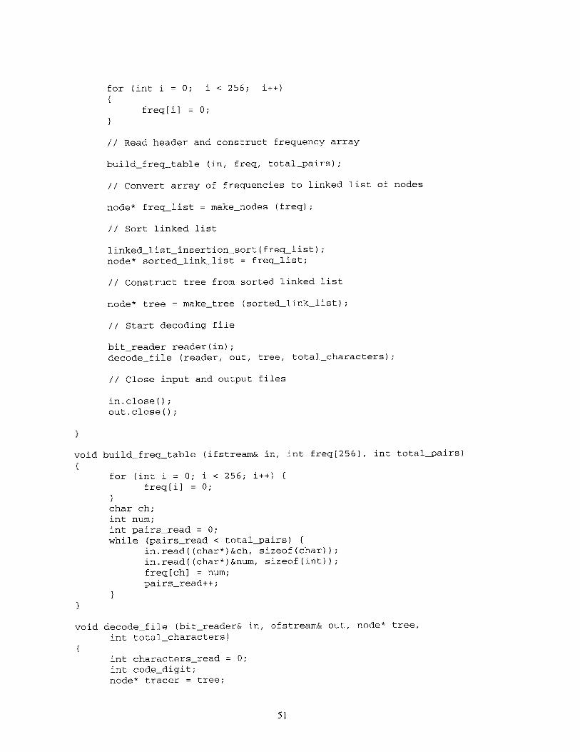
void buildfreqtable (ifstream& in, int freq[256), int total-pairs);

void decode file (bitreader& in, ofstream& out, node* tree, int

totalcharacters);

/* main procedure for decompression. Takes command line arguments.

* To use, type: ./puff input-file-name output-file-name at prompt */

int main(int argc, char **argv)

{ifstream in;ofstream out;

/* Check for file name on the command line */

if (argc == 3) (in.open(argv[1], ios::binarylios::in);

out.open(argv[2], ios::binaryjios::out);

if (!in || !out) {

cerr << "Can't open file!\n";

exit(0);

}}else {

cerr << "Usage: puff <input fname> <output fname>\n";

exit(0);

// Read in first int which indicates total number of encoded

characters

int totalcharacters;in.read((char*)&totalcharacters, sizeof(int));

// Read in second int which indicates total number of char/code

pairs

int total-pairs;in.read((char*)&totalpairs, sizeof(int));

int freq[256];

50

for (int i = 0; i < 256; i++)

{freq[i] = 0;

}

// Read header and construct frequency array

buildfreqtable (in, freq, totalpairs);

// Convert array of frequencies to linked list of nodes

node* freqlist = makenodes (freq);

// Sort linked list

linkedlistinsertion-sort(freqjlist);node* sortedlinklist = freqlist;

// Construct tree from sorted linked list

node* tree = maketree (sortedlinklist);

// Start decoding file

bitreader reader(in);

decodefile (reader, out, tree, totalcharacters);

// Close input and output files

in.close(;out.close(;

}

void build freqtable (ifstream& in, int freq[256], int total-pairs)

{for (int i = 0; i < 256; i++) {

freq[i] = 0;

}char ch;int num;int pairsread = 0;while (pairsread < total-pairs) {

in.read((char*)&ch, sizeof(char));

in.read((char*)&num, sizeof(int));

freq[ch] = num;pairs-read++;

}}

void decodefile (bitreader& in, ofstream& out, node* tree,

int total-characters)

{int charactersread = 0;

int code-digit;node* tracer = tree;

51

while (charactersread < totalcharacters) (while (tracer -> right != NULL && tracer -> left NULL) {

bool success = in.getbit(codedigit);

if (!success)return;

}if (codedigit == 0) {

tracer = tracer -> left;

}else {

tracer = tracer -> right;

}}out.write((char*)&(tracer->character), sizeof(unsigned

char));tracer = tree;charactersread++;

}}

52

/* File: utils.h* Author:Wang-Rei Tang* JoRel Sallaska* Common routines to manipulate huffman encoding data structures*/

#ifndef _UTIL_H#define _UTIL_H

#include <iostream.h>#include <iomanip.h>#include "bits.h"

struct node {unsigned char character;int frequency;node* next;

node* left;node* right;

node* makenodes(int freq[]);void linkedlistinsertion-sort (node* &freq-list);

void insertionsort (node* &tree);

node* combine_2_nodes (node* a, node* b);

node* maketree (node* first-node);

void buildkey (code mycodes[ ], node* tree, code& thecode);

void writebit (int bit, code& thecode);

void erasebit (code& thecode);

void traversetree (node* tree, code mycodes[], code& thecode);

void printtree(node* tree);

#endif

}

53

/* File: utils.cc* Author:Wang-Rei Tang* JoRel Sallaska* Common routines to manipulate huffman encoding data structures

*/

#include <iostream.h>#include <iomanip.h>

#include <assert.h>

#include "utils.h"#include "bits.h"

void printtree (node* tree) {

if (tree == NULL)

return;

cout << "Node: " << tree->character << endl;

cout << "frequency: " << tree->frequency << " next:

<< (unsigned int)tree->next << " left: " << (unsigned int)tree-

>left<< " right: " << (unsigned int)tree->right << endl;

print-tree (tree->left);print-tree (tree->right);

}

// Makes linked list of nodes from frequency array

node* make nodes(int freq[]) {node* head;node* curr;curr = new node;head = curr;for (int i = 0; i < 255; i++) {

if (freq[i] == 0){continue;

}curr -> character = char (i);

curr -> frequency = freq[i];curr -> next = new node;curr->left = NULL;curr->right = NULL;curr = curr -> next;

}curr -> character = char (255);

curr -> frequency = freq [255];

curr -> next = NULL;curr->left = NULL;

curr->right NULL;

return head;

}

// Sorts list of nodes

void linkedlistinsertion-sort (node* &freqjlist) {

node* ptr = freq_list;node* nextnode = ptr -> next;

54

while (next-node -> next != NULL) {

// Go to first element that is out of order

while (ptr -> frequency <= nextnode -> frequency

&& nextnode -> next NULL) {

ptr = next-node;nextnode = nextnode -> next;

}

// If not at end of list, move element out of order to begninning of

// list and call insertion sortif (ptr -> frequency > nextnode -> frequency) {

ptr -> next = nextnode -> next;

nextnode -> next = freq_list;

freqlist next-node;insertion sort(freq_list);nextnode = ptr -> next;

}}if (ptr -> frequency > nextnode -> frequency) {

ptr -> next = NULL;

nextnode -> next = freqjlist;freq_list = nextnode;insertionsort(freq_list);

}}

// Finds appropriate spot in linked list for first node and inserts it

void insertionsort (node* &tree) {

if (tree -> next != NULL) {

if (tree -> frequency <= tree -> next -> frequency) {return;

}node* head = tree -> next;node* ptr = head;node* last = tree;while (ptr -> frequency < tree -> frequency && ptr -> next

NULL) {last = ptr;ptr = ptr -> next;

}if (ptr -> frequency < tree -> frequency && ptr -> next == NULL)

{ptr -> next tree;tree -> next = NULL;

tree = head;return;

}tree -> next = last -> next;

last -> next = tree;

tree = head;

}

// Combines 2 nodes into parent w/ children and returns pointer to

parent

55

node* combine_2_nodes (node* a, node* b) {

node* parent = new node;parent -> frequency = a -> frequency + b -> frequency;

if (a -> frequency <= b -> frequency) {parent -> left = a;parent -> right = b;

}else {

parent -> left = b;parent -> right = a;

}parent -> next = b -> next;

a -> next = NULL;b -> next = NULL;return parent;

}

// Combines linked list of nodes into huffman tree and returns pointer

to// top of tree

node* maketree (node* first-node) {

node* tree;while (firstnode -> next != NULL) {tree = combine_2_nodes (first-node, firstnode -> next);

insertionsort (tree);

firstnode = tree;}return tree;

}

// Given array for key and pointer to tree, stores all codes in array

key.

void build key (code mycodes[], node* tree, code& thecode) {

traversetree (tree, mycodes, thecode);

}

// Adds one bit to end of thecode with the value bit.

void write bit (int bit, code& thecode) {

thecode.bits = (thecode.bits << 1) I bit;thecode.length++;

}

// Takes one bit from end of thecode.

void erase bit (code& thecode) {

thecode.bits = thecode.bits >> 1;

thecode.length--;

}

// Traverses tree & stores all codes and length of codes in array of

all codes

56

void traversetree (node* tree, code mycodes[], code& thecode) {

if (tree -> left == NULL && tree -> right == NULL) {mycodes [int(tree -> character)].bits = thecode.bits;

mycodes [int(tree -> character)].length = thecode.length;return;

}write-bit(O, thecode);traversetree (tree -> left, mycodes, thecode);

erasebit (thecode);write-bit (1, thecode);

traversetree (tree -> right, mycodes, thecode);

erase-bit (thecode);return;

57

CHPATER NINE CONCLUSION

Data compression algorithm is a set of rules and procedures used to compress an

original file into a smaller destination file represented by fewer bits (for the purpose of

efficient storage) and to decompress the destination file into the original file when it is

needed. An efficient data compression algorithm has a higher compression ratio, saves

more storage space, or increases the speed of downloading files on the Internet. It is very

important because saving time and space usually means saving money.

The variety of data compression algorithms is almost endless. There are many

ways to group data compression algorithms into a few classes based on the techniques

used to do compression. In fact, a lot of algorithms are developed from more than one of

the classes.

Run-length coding is one of the simplest data compression algorithms. Run-

length coding replaces sequences of consecutive identical data items with three elements:

a control symbol, a run-length count and a data item. It is highly effective when there are

a lot of runs of consecutive symbols. But in plain English text, there are not many

repetitions.

The different Run-length encoding variants have one common feature: they

assign fixed-size codes to the symbols on which they operate. In contrast, statistical

encoding takes advantage of the probabilities of occurrence of single characters and

groups of characters, so that short codes can be used to represent frequently occurring

characters or groups of characters while longer codes are used to represent less frequently

58

encountered characters and groups of characters. Shannon-Fano encoding, the Huffman

code and arithmetic coding are all in the family of statistical methods.

Huffman coding shares most characteristics of Shannon-Fano coding. Symbols

with higher probabilities get shorter codes. They both have the unique prefix property

and produce the best codes when the probabilities of the symbols are negative powers

of 2. However, building a Huffman decoding tree is done using a completely different

algorithm from that of the Shannon-Fano method. The Shannon-Fano tree is built from

the top down, and the Huffman tree is built from the bottom up. One of the problems

associated with the development of the Shannon-Fano code is the fact that the procedure

to develop the code can be changeable. It is important where we make a split in the

subset construction process. Huffman coding solves the problem. It assigns the optimal

unambiguous encoding to the symbols.

In Huffman coding, when several symbols have the same frequency of

occurrence, we may be able to develop two or more sets of codes to represent Huffman

coding. The rule is to always combine the lowest frequency with the highest frequency

while merging the symbols' probabilities. As stated earlier, the Huffman code is only

optimal when all symbol probabilities are negative powers of 2. In practice, this situation

is not guaranteed to occur. Huffman code can be generated no matter what the symbol

probabilities are, but they may not be efficient. Arithmetic encoding solves this problem.

Using arithmetic coding, a message is encoded as a real number in an interval

from zero to one. Unlike Huffman coding, arithmetic coding takes the whole message

from the input stream and encodes it into one code. It creates a single symbol rather than

59

several separate codes. Arithmetic coding typically gives better compression ratios than

Huffman coding. It is a more recent technique compare to Huffman coding.

Dictionary-based methods do not use a statistical model, nor do they use variable-

size codes. Instead, they select strings of symbols and encode each string as a token

using a dictionary. LZ 77 (Sliding Window) and LZ 78 are in the family of dictionary-

based methods. Dictionary-based methods were not mentioned in the paper. It will be

noted in a future work. All the algorithms mentioned in this paper were for symbolic

data compression. In the future work, image compression, video compression, and audio

compression shall be covered.

60

APPENDIX A

/* File: bits.h

* Author: Omri Traub <otraub@eecs.harvard.edu>*

* Routines for reading and writing bits to a file.

* NOTE: you should not have to modify this file.*/

#ifndef _BITS_H#define _BITS_H

#include <iostream.h>#include <iomanip.h>#include <fstream.h>

/* An encoding of a character consists of the bits and the number of

* bits in the code.

* Note: you are encouraged to use this class whenever you need

* to store a bit code */

class code {public:

code() { bits = length 0; }

unsigned int bits;

int length;

};

/* A class interface to reading a file one bit at a time */

class bitreader {public:

/* initialize the reader with an input file handle */

bitreader(ifstream &_in);

/* read the next bit from the file into the argument int

variable.* returns a bool indicating whether eof reached */

bool getbit(int &the-bit);

private:/* a bit buffer containing up to 8 bits from the file */

unsigned char buffer;

/* how many character are currently in the buffer */

int bufjlen;

/* the current file, assumed to be open */

ifstream *in;

/* A class interface to writing a file one bit at a time */

class bitwriter {

public:/* initialize the reader with an output file handle */

bitwriter(ofstream &_out);

61

/* write the next code (sequence of bits) to the file */

void writecode(code thecode);

/* write the next bit to the file. */

void put-bit(int the-bit);

/* when the buffer gets full, write the bits out to the file.

* NOTE: call this file when you are done writing, or else some

bits* may not get written out! */void flushbits();

/* return the number of bytes written to file */

int numbyteswritten() { return num-bytes; }

private:/* a bit buffer containing up to 8 bits to be written to the file

*/unsigned char buffer;

/* how many character are currently in the buffer */

int bufjlen;

/* the current file, assumed to be open */

ofstream *out;

/* number of bytes written */

int num-bytes;

};

#endif

62

/* File: bits.cc* Author: Omri Traub <otraub@eecs.harvard.edu>*

* Routines for reading and writing bits to a file.

* NOTE: you should not have to modify this file.*/

#include <iostream.h>#include <iomanip.h>#include <fstream.h>#include "bits.h"

/* initialize the reader with an input file handle */

bitreader::bitreader(ifstream &_in)

{in = &_in;

buffer = buflen = 0;

}

/* read the next bit from the file into the argument int variable.

* returns a bool indicating whether eof reached */

bool bitreader::get-bit(int &thebit)

{/* buffer is empty: need to read more bits from the file! */

if (buflen == 0) {buffer = in->get(;if (in->eof()return false; /* that's it! eof has been reached */

/* just read 8 bits */

buflen = 8;}

/* now we need to get the highest bit that is valid:

* i.e. the bit in position buflen - 1 in the buffer */

thebit = (buffer & (1 << (buflen-1))) >> (buf_len - 1);

buflen--;

return true;

}

/* initialize the reader with an output file handle */

bitwriter::bit_writer(ofstream &_out)

{out = &_out;

buffer = buflen = num-bytes = 0;

}

/* write the next code (sequence of bits) to the file */

void bitwriter::writecode(code the-code)

{

63

int i;int bit;

/* call put-bit() on all bits, from left to write */for (i = thecode.length-1 ; i >= 0; i--) {bit = (the-code.bits & (1 << i)) >> i;put-bit(bit);}

}

/* write the next bit to the file. */void bitwriter::put-bit(int thebit)

{/* if the buffer has eight bits, need to flush it first */

if (buflen == 8) {flushjbits();

}

/* need to add the new bit to the right of exisiting buffer */

buffer = (buffer << 1) the-bit;

buf-len++;

}

/* when the buffer gets full, write the bits out to the file.

* NOTE: call this file when you are done writing, or else some bits

* may not get written out! */

void bitwriter::flushbits()

{/* if buffer has fewer than 8 bits, need to shift the bits

* left to align them with the left end of the byte before

* writing out. NOTE: when you read in the bits, there may be

some* extra 0 bits dangling at the end! */

if (buflen < 8)buffer = buffer << (8 - buflen);

out->put(buffer);

buffer = buflen= 0;

num-bytes++;

}

64

REFERENCES

David, Salomon. Data Compression - The Complete Reference. Springer-VerlagNew York, Inc. 1998

Roy, Hoffman. Data Compression in Digital System. Chapman & Hall, 1997

Gilbert, Held. Data and. Image Compression - Tools and Technique. John Wiley &Sons Ltd, 1996

Mark, Nelson. The Data Compression Book. M&T Books. 1992

http://www.rasip.fer.hr/research/compress/

http://lena.cs.utu.fi/tko/reports/R-92-6.html

http://www.zipworld.com.au/-isanta/uni/arithmetic.htm

http://ltssg3.epfl.ch/pub-files/brigger/thesishtml/node94.html

http://www.eas.asu.edu/morrell/551fall95/project1/projectl.html

http://student.monterey.edu/dh/dunkeljodyd/world/cst332/alpresent/ 1O.htm

http://www.mdc.net/~eberhard/ari/arithmetic.html

http://www.ics.uci.edu/-dan/pubs/DC-Sec3.html#Sec_3.1

http://www.eee.bham.ac.uk/WoolleySI/A1l7/huff_1.htm

http://www.eee.bham.ac.uk/WoolleySI/All7/HuffTutorial.htm

http://www.compressconsult.com/huffman/

http://www.ee.uwa.edu.au/-plsd21/ds/huffman.html

65