the open chemical engineering journal€¦ · · 2017-11-09the open chemical engineering journal,...

Send Orders for Reprints to [email protected]

The Open Chemical Engineering Journal, 2017, 11, 33-52 33

1874-1231/17 2017 Bentham Open

The Open Chemical EngineeringJournal

Content list available at: www.benthamopen.com/TOCENGJ/

DOI: 10.2174/1874123101711010033

RESEARCH ARTICLE

Modeling and Simulation of Pressure Equalization Step Between aPacked Bed and an Empty Tank in Pressure Swing Adsorption Cycles

Mohamed Hachemi Chahbani1,2,*, R. Talmoudi2,3, Amna Abdel Jaoued2,3 and D. Tondeur4

1Institut Supérieur des Sciences Appliquées et de Technologie de Gabès, Université de Gabès, Rue Omar Ibn Elkhattab,Zrig, Tunisia2Laboratoire Génie des procédés et systèmes industriels (LR11ES54), Université de Gabès, Rue Omar Ibn Elkhattab,Zrig, Gabès 6029, Tunisia3Ecole Nationale d'Ingénieurs de Gabès, Université de Gabès, Rue Omar Ibn Elkhattab, Zrig, Gabès 6029, Tunisia4Laboratoire Réactions et Génie des Procédés, CNRS et Université de Lorraine, ENSIC, 1 Rue Grandville- 54000Nancy - France

Received: May 30, 2017 Revised: June 01, 2017

Abstract:

Background:

It is of paramount importance to pay a great attention when modeling pressure equalization step of pressure swing adsorption cyclesfor its notable effect on the accurate prediction of the whole cycle performances. Studies devoted to pressure equalization between anadsorption bed and a tank have been lacking in the literature. Many factors could affect the accuracy of the dynamic simulation ofpressure equalization between a bed and an empty tank.

Methods:

The method used for the equilibrium pressure evaluation has a significant impact on simulation results. The exact equilibriumpressure (Peq) obtained when connecting an adsorption column and an empty tank could only be obtained by numerical simulationgiven the complexity of the set of partial differential equations.

Results:

It has been shown that, with some simplifying assumptions, one can analytically determine Peq with satisfactory precision. Theanalytical solution proposed permits to assess rapidly the equilibrium pressure and the equilibrium mole fraction of the adsorbablespecies in the tank (Yeq) and without the need to resort to a cubersome modeling.

Conclusion:

Based on the comparisons presented, one can conclude that the agreement between the experimental and numerical results relative toPeq and Yeq is very satisfactory.

Keywords: Pressure equalization step, Equilibrium pressure, Empty tank, Modeling, Dynamic simulation, Pressure swingadsorption.

1. INTRODUCTION

The modeling of varying pressure steps of pressure swing adsorption cycles have received a great deal of attentionbecause of the great effect of these steps on the accurate prediction of whole cycle performances. These steps comprise

* Address correspondence to this author at the Institut Supérieur des Sciences Appliquées et de Technologie de Gabès, Université de Gabès, RueOmar Ibn Elkhattab, Zrig, Gabès 6029, Tunisia; Tel: (216) 98 944 632; E-mail: [email protected]

Accepted: August 20, 2017

http://benthamopen.com

http://crossmark.crossref.org/dialog/?doi=10.2174/1874123101711010033&domain=pdf

http://www.benthamopen.com/TOCENGJ/

http://dx.doi.org/10.2174/1874123101711010033

mailto:[email protected]

34 The Open Chemical Engineering Journal, 2017, Volume 11 Chahbani et al.

pressurization, blowdown and equalization. However, until recently, the main attention has been given to pres-surization and depressurization. The incorporation of a pressure equalization step has been proposed for the first time byBerlin in 1966 [1]. The pressure equalization step has two purposes: To save the mechanical energy contained in the gasof a high pressure bed, and to recover a part of the product that would otherwise be lost in the blowdown. One of theways to do this is to use the high-pressure gas removed during the cocurrent depressurization step to repressurize otheradsorber by pressure equalizations. It is done by connecting the ends of two beds at a particular stage of the cycle. Thus,pressure equalization steps enable gas separations to be realized economically on a large scale.

Very few articles entirely devoted to the study of the equalization step of PSA cycles have been published. Apartfrom some adsorption simulators, capble of simulating the step with no simplifying assumptions such as ASPENAdsorption, the equalization step has been generally treated as an ordinary depressurization for the high pressure bed(from PH to Peq ) and as an ordinary pressurization for the low pressure bed (from PL to Peq ) with a constant pressure atthe open end of the bed (Peq ). The equilibrium pressure Peq reached at the end of the equalization step is evaluated afterconsidering simplifying assumptions and rough approximations [2 - 5]. In many approaches, the pressure history duringequalization is assumed to follow some simple law, e.g. exponential or linear, similarly to the conventionaldepressurization or pressurization steps.

Warmuzinski [6] has developed a simple analytical formula to measure energy savings resulting from the pressureequalization step. Warmuzinski and Tanczyki [7], have also proposed a formula for calculating the equilibrium pressurePeq in the case of linear uncoupled isotherms and no breakthrough of the more strongly adsorbed component from thebed undergoing depressurization. Delgado and Rodrigues [8] have analyzed the effect of three types of boundaryconditions on the time and spatial profiles of the pressure equalization step of a Skarstrom PSA cycle. Chahbani andTondeur [9] have simulated the dynamics of the pressure equalization step and evaluated the equilibrium pressurenumerically and analytically.They have shown that in some simple cases only the pressure equalization step can bedecomposed into independent pressurization and depressurization steps and that the constant pressure at the open end ofthe pressurized or depressurized bed should be accurately estimated prior to this decomposition. Yavary et al. [11] havefound that the analytical solution, proposed by Chahbani and Tondeur for the evaluation of the equilibrium pressure,provides a more realistic mathematical procedure with respect to the use of an arithmetic mean for the calculation of thefinal pressure for the pressure equalization steps. Yavary et al. [12] have also shown that the number of pressureequalization steps affects significantly both purity and recovery of product. Therefore, the number of pressureequalization steps must be considered as an important process parameter in evaluating process performance.

In 1964, prior to Berlin’s improvement of the Skarstrom cycle, Marsh et al. [10] have suggested another idea forreducing blowdown loss. Besides the two adsorption beds, an empty tank is used. At the end of the high-pressureadsorption step but well before breakthrough, the feed flow is stopped and the product end of the high-pressure bed isconnected to the empty tank where a portion of the compressed gas, rich in the product, is stored. The blowdown of thehigh-pressure bed is completed by venting to the atmosphere in the reverse-flow direction. The stored gas is then usedto purge the bed after which the bed is finally purged with product gas. The product comsumption during purge isreduced, thereby increasing the recovery. Tondeur and Wankat [13] have described a number of PSA cycles thatimplement empty tanks, and have shown that the sequences in complex multi-column, multi-step cycles can beemulated by a system comprising a single column and a multiplicity of empty tanks. It is therefore of general interest torevisit the pressure equalization between a column and an empty tank.

In the work previously cited, we have studied in detail pressure equalization between two packed columns. In thiswork, we will try to extend the previous study to pressure equalization between a column and a tank in the sense thatstudies devoted to pressure equalization with a tank have been lacking in the literature.

2. MODELING

The simulation of a fixed-bed adsorber requires the numerical solution of the governing partial differentialequations: mass, heat and momentum balances as well as mass transfer kinetics.

2.1. Mass Balance for the Packed Bed

A differential fluid phase mass balance for the component i is given by the following axially dispersed plug flowequation:

Modeling and Simulation of Pressure Equalization The Open Chemical Engineering Journal, 2017, Volume 11 35

(1)

with ϵt = ϵ + (1 − ϵ) ϵp, being the total porosity.

The overall mass balance for the bulk gas is given by:

(2)

wherein u is the interstitial fluid velocity, ϵ the bed or the interparticle void fraction,ϵp the intraparticle void fractionor porosity, the total bulk phase concentration, Z being the compressibility factor of the gas mixture.

2.2. Heat Balance for the Packed Bed

A heat balance for the bed can be written as:

(3)

with

For completeness, this equation accounts for heat transfer between the column and some environment at atemperature Te. However, in the numerical application, only the adiabatic case will be considered. In the following, theheat capacities of adsorbed species (cpi

a ) are supposed to be equal to those in gas phase (cpig ).

2.3. Momentum Balance

Ergun’s law is used to estimate locally the bed pressure drop.

(4)

where µ is the gas mixture viscosity, ρ the gas density and dp the particle diameter.

2.4. Mass Balance for the Empty Tank

A fluid phase mass balance for the component i in the tank is given by the following equation:

(5)

is the volume flowrate at the tank inlet which is equal to the volume flowrate at the bed exit,

is the gas velocity at the bed outlet. and are the concentrations of gas component i at the tank inlet and inthe tank respectively. The tank is considered perfectly mixed.

ϵt∂Cyi∂t

+ (1− ϵ)∂qi∂t

+∂(ϵ u Cyi)

∂z=

∂

∂z(ϵDaxC

∂yi∂z

)

ϵt∂C

∂t+ (1− ϵ)

Ng∑i=1

∂qi∂t

+∂(ϵ u C)

∂z= 0

ϵm∂(C Ug)

∂t+ (1− ϵ)

(ρs∂Hs

∂t+

Ng∑i=1

qi∂H i

a

∂t

)

+(1− ϵ)∂(u C Hg)

∂z− (1− ϵ)

Ng∑i=1

∆H i∂qi∂t

+4h

Dcol

(T − Te) = 0

Ug = Hg −P

C, dHg =

Ng∑i=1

yi cpigdT, dH i

a = cpiadT, dHs = cpsdT

−∂P

∂z= 150.0

(1− ϵ)2

ϵ2µ

d2pu+ 1.75

1− ϵ

ϵ

ρ

dpu2

Vtank∂Ctank

i

∂t= Qtank

in Ctanki,in

Qtankin = ϵ S ubed

out ubedout

Ctanki,in Ctank

i

C =Z P

R T


2.5. Heat Balance for the Empty Tank

A heat balance for the tank can be written as:

(6)

with , the gas concentration and the gas internal energy in the tank, and the gasconcentration and the gas enthalppy at the tank inlet, Stank the heat transfer surface of the tank.

2.6. Numerical Method

The foregoing models require the simultaneous solution of a set of partial differential and algebraic equations(overall and component mass balance equations, heat balance equation and momentum balance equation). The aboveequations are easily rewritten using dimensionless variables, (P/Pref , u/uref ,T /Tref, ............). The well-mixed cellsmethod is used to discretize the system. The resulting system of ordinary differential and algebraic equations aresolved by the DDASSL integration algorithm of Petzold [14] DASSL is designed for the numerical solution of implicitsystems of differential/algebraic equations written in the form F(t,y,y’)=0, where F, y, and y’ are vectors, and initialvalues for y and y’ are given. The time derivatives are approximated by the Gear formula BDF (BackwardDifferentiation Formula) and the resulting nonlinear system at each time-step is solved by Newton’s method. The fulldescription of the code can be found in reference [14]. The runtime of the code is less than one minute for an ordinarycomputer equipped with Intel Core 2 Duo Processor E4700 (2M Cache, 2.60 GHz, 800 MHz FSB).

2.7. Boundary and Initial Conditions

As shown in Fig. (1), the boundary conditions are as follows:

The whole step can be considered as a depressurization of the bed and a pressurization of the tank. The pressure atthe outlet of the bed or at the inlet of the tank varies with time.

Fig. (1). Schematic representation of the equalization step.

The initial conditions for the bed and the tank should also be defined. The pressure is PH in the bed and PL in thetank. The axial profiles of composition and temperature at t = 0 in the bed correspond to those of the final state attainedduring the step preceding the equalization step.

The effluent of the column is the feed of the tank. Thus, pressure, temperature and composition at the outlet of thebed are identical to those prevailing at the inlet of the tank.

This paper will only focus on the assessment of the equilibrium pressure obtained when connecting an adsorptioncolumn and a tank and will not deal with energy consumption optimization and product recovery. In fact, one of thegoals of the equalization step is to collect the portion of product-rich gas ahead of the concentration wave (in the masstransfer zone). The amount of gases transferred to the tank strongly depends on the initial location of the concentrationwave. In a real situation, the optimized tank volume is related to the initial location of the concentration wave front inthe bed. The best situation would be that the adsorbable species is just about to breakthrough when the pressure isequalized. The packed bed is initially uniformly loaded. The reason of starting the simulation from a uniformly loaded

Vtank

∂(Ctank U tankg )

∂t= Qtank

in Ctankg,in H tank

g,in − h Stank (Ttank − Te)

- At z = 0, ∂yi∂z

= 0, ∂T∂z

= 0, ∂P∂z

= 0 ∀ t

-At z = L, ∂yi∂z

= 0, ∂T∂z

= 0, P = P tank(t) ∀ t

empty tankadsorption bed0=z Lz =

HP LP

Ctank,U tankg Ctank

g,in H tankg,in


bed is that it would be easy, as we shall see later when the bed is initially uniformly loaded, to validate the experimentscarried out without having to worry about the precise position of the front in the column before the pressureequalization step. The validation is simply done through the comparison of the values of the equilibrium pressure andthe molar fraction of the adsorbable gas in the tank at the end of the step obtained numerically and experimentally.

In practical operations, the column and the tank are separated by valves and tubings, which could in principle beincluded in the modeling. The work presented herein considers that the pressure drop through the valves and tubings isnegligible. This does not affect the value of equilibrium pressure attained at the end of the step, it does only modify thedynamics of the pressure equalization. in fact, the presence of significant pressure drop tends to increase the duration ofthe step.

When flow goes through a valve or any other restricting device, it loses some energy. The flow coefficient (cv ) is adesigning factor which relates pressure drop (∆P) across the valve with the flow rate (Q). Each valve has its own flowcoefficient. This depends on how the valve has been designed to let the flow going through the valve. Therefore, themain differences between different flow coefficients come from the type of valve, and of course the opening position ofthe valve. At same flow rate, higher flow coefficient means lower drop pressure across the valve. Depending ofmanufacturer and type of valve, the flow coefficient can be expressed in several ways.

Simulating of varying pressure steps without the incorporation of a valve equation shows a notable disparity withexperimental results as can be seen in Fig. (2) for depressurization. This is why it is indispensible to take into accountthe significant pressure drop across the valve in the modeling. The two following valve models could be used:

Fig. (2). Variation of the pressure at the closed end of the column during depressurization: Comparison between experimentalresults and simulation without valve model, PH = 10 bars, L = 1 m, Dcol = 5 cm.

Q = cu ∆P [15].1.

Q = cu [16].2.

avec

C concentration (mol/m3)Q molar flow rate (mol.s−1)∆P pressure drop across the valve (Pa)

Figs. (3 and 4) show that the incorporation of a valve equation in the modeling permits to obtain a good agreementbetween experimental results and simulations. The values of the flow coefficients given by the two models are different.However, it must be noted that the values of flow coefficients obtained herein are only valid for the experimental PSAsetup studied and they can not be used for simulating different theoretical PSA systems.

2

4

6

8

10

0 0.5 1 1.5 2 2.5

P(B

AR

S)

t(s)

EXPERIMENTAL DATASIMULATION

√C ∆P


Fig. (3). Variation of the pressure at the closed end of the column during depressurization: Comparison between experimentalresults and simulation for various values of cv , valve: Model 1, the arrow indicates increasing values of cv , PH =10 bars, L = 1 m,Dcol = 5 cm.

Fig. (4). Variation of the pressure at the closed end of the column during depressurization: comparison between experimentalresults and simulation for various values of cv , valve: model 2, the arrow indicates increasing values of cv , PH = 10 bars, L = 1 m,Dcol = 5 cm.

However, it should be mentioned that, in the following, a valve equation will be only used when comparingsimulation and experimental results. As previously mentioned, the assessed equilibrium pressure is not affected by thepresence or absence of a valve equation in the modeling.

2.8. Analytical Solution for the Equilibrium Pressure

As presented above, the model can not be analytically solved. However, if the following simplifying assumptionsare considered, an analytical solution can be obtained. For the purpose of comparison, we shall examine the results ofthis analytical approximation as well as the full numerical solutions:

The process is isothermal1.The column and the tank are considered homogeneous at the initial and final states.2.

2

4

6

8

10

0 2 4 6 8 10 12

P(B

AR

S)

t(s)

cv=

EXPERIMENTAL DATA2.0 10-6

5.0 10-6

1.1 10-5

2.0 10-5

2

4

6

8

10

0 2 4 6 8 10 12

P(B

AR

S)

t(s)

cv=

EXPERIMENTAL DATA5.0 10-8

1.0 10-7

2.6 10-7

5.0 10-7


The gaseous and solid phases are in equilibrium at the initial and final states.3.The equalization time is large.4.

The fourth condition implies that the column and the tank become identical at the end of the equalization step. Thisapproximation may appear very rough, but as will be seen later, the value of the equalization pressure obtainedconsidering these hypotheses is more accurate than the arithmetic or geometric mean.

For the sake of simplicity, the resolution is restricted to the case of a gas mixture composed of two species, one ofwhich is inert (I) whereas the other is adsorbable (A).

The total number of moles in each bed at the initial state are

(7)

and

(8)

Where ϵt is the total porosity (ϵ + (1 − ϵ)ϵp). The first term on the right hand side represents the moles adsorbed. Inequations (7) and (8), the subscript 0 refers to the initial state.

The constitutive equations of the model are written as follows:

-Conservation of the total number of moles in the the column

(9)

Where the total number of moles in the system n is given by the sum of Equations (7) and (8). The subscript eqrefers to the end of the equalization step.

-Conservation of the total number of moles of inert component I

(10)

-Langmuir adsorption equilibrium in column 1 after equalization :

(11)

-Summation of mole fractions in the column

(12)

-Summation of mole fractions in the tank

(13)

The system of 5 equations (9) to (13) relates 6 unknowns (the four mole fractions y, the adsorbed quantity qcoleq and

Peq ). By substituting equations (11) to (13) into Equations (9) and (10), three of these variables can be eliminated,leaving a system of two equations with three unknowns, Peq , y

coleqI and ytank

eqI for example. To resolve analytically, anadditional assumption needs to be made. We shall assume here that the column and the tank have identical gas phasecompositions at the end of equilibration (thus, ycol

eqI = ytankeqI ), leaving only two unknowns. The analytical resolution

then leads to a quadratic equation whose positive root is

ncol0 = ρb Vcol qcol0 + ϵt

Vcol PH

R T

ntank0 =

Vtank PL

R T

n0 = ϵtVcol Peq

R T+ ρb Vcol qcoleq +

Vtank Peq

R T

n0I = ϵtVcol Peq

R TycoleqI

+Vtank Peq

R TytankeqI

qcoleq =Qm b Peq y

coleqA

1 + b Peq y1eqA

ycoleqA+ ycoleqI

= 1

ytankeqA+ ytankeqI

= 1

:

:


(14)

with

where

The inert species molar fraction is:

(15)

The adsorbable species molar fraction is

(16)

In the case of more than one adsorbable species, a similar set of conservation and equilibrium equations may bewritten, and with the assumption of equal gas-phase compositions of the columns and the tank in the end state, this setdetermines the end pressure Peq. However, a compact analytical solution is probably impossible, and the solution forPeq has to be found numerically.

In the case where the column and the tank initially contain only one species (adsorbable or inert), one can easilyobtain the following formula for the equilibrium pressure

(17)

If the column and the tank have the same volume Peq becomes:

(18)

3. RESULTS AND DISCUSSION

The numerical simulations presented herein concern methane uptake from hydrogen by using activated carbon. H2 issupposed to be a non-adsorbed species. The adsorption equilibrium isotherm of CH4 on activated carbon is given by theLangmuir model

(19)

Peq =−B +

√B2 − 4 A C

2 A

A =(Vtank + ϵtVcol) b

R T

B = ρbVcol qm b+(Vtank + ϵtVcol)

R T(1− b α)− β b

C = −β (1− α b)− ρbVcol qm b α

α =ϵt Vcol PH ycol0I

+ Vtankl PL ytank0I

Vtankl + ϵt Vcol

β = ρb Vcol qcol0 + ϵt

Vcol PH

R T+

VtankPL

R T

yeqI =α

Peq

yeqA = 1− α

Peq

Peq =ϵt Vcol PH + Vtank PL

Vtank + ϵt Vcol

Peq =ϵt PH + PL

1 + ϵt

:

Q∗ =Qm b yi P

1 + b yiP


The parameters Qm and b are function of temperature:

(20)

(21)

Table 1 gives the values of ki parameters and adsorption heat used in simulations.

Table 1. Langmuir parameters and adsorption heat [9].

Langmuir parametersk1 7.063 103 mol/m3

k2 13.610 mol/(m3K)k3 3.07110−8 1/Pak4 1574.1 K

Adsorption heat (∆H) 20.0 kJ/mol

The model requires the assessment of the physical properties of the gas mixture. The compressibility factor iscalculated following the method of Lee-Keesler [17]. The viscosity of each pure gas is estimated by Lucas method [17]whereas the viscosity of the mixture is evaluated by the Reichenberg method [17]. The compressibility factor (Z), themixture viscosity (µ) as well as the gas density (ρ) vary with temperature, pressure and composition, therefore they arecalculated at every computation step.

The adsorbent physical properties are given in Table 2. The heat capacities of the various gases are calculated byusing an equation of the following form:

(22)

Table 2. Adsorbent physical properties [9].

Apparent density (ρp) 830 kg/m3

Intraparticle porosity (ϵp) 0.6Particule diameter (dp)

0.1 10−3 mHeat capacity (cps) 1.050 kJ/(kg K)

The constants a, b, c and d for the two gases are listed in Table 3.

Table 3. a, b, c and d constants for the calculation of heat capacities [9].

a b c dH2 27.14 9.274 10-3

-1.381 10-5 7.645 10-8 CH4 19.25 5.213 10-2

1.197 10-5 -1.132 10-8

Table 4 gives the operating conditions used for computations. All the following simu-lations are in the adiabaticcase (h=0).

Table 4. Operating conditions used in the simulations.

Initial pressure (P)Bed 5.0 105 PaTank 1.0 105 Pa

Initial temperature 298 KInitial CH4 mole fraction

In the bed 0.5In the tank 0.0 (pure hydrogen)

Qm = k1 − k2T

b = k3 exp(k4T)

Cp(J/(mol.K)) = a+ b T + c T 2 + d T 3


Initial pressure (P)Bed length (L) 2.0 mInterparticle porosity (ϵ) 0.4

In what follows, we will consider a fully saturated column at a high pressure PH and a tank at a low pressure PL

containing only inert (pure product). The volume of the tank is equal to that of the column. Fig. (5) gives the evolutionof the pressure in the column and the tank during time. The pressure in the tank, as mentioned previously, is uniform.X-coordinates (z/L) varying from 0.0 to 1.0 correspond to the column, and x-coordinates from 1.0 to 2.0 are relative tothe tank. This does not mean that the tank has the same length as the column.This representation is chosen to show boththe pressure variation in the column and the tank, since the numerical solution gives only a single pressure value in thetank and not a longitudinal profile.

Fig. (5). Evolution of axial profiles of reduced pressure in the bed and in the tank for different times (∆t = 0.25 s) during pressureequalization step,PH = 5.0 bars, PL = 1.0 bar Pref = 5.0 bars.

The reference pressure is taken as Pref = PH . The reference velocity uref is calculated using Ergun’s correlation asfollows:

(23)

The pressure in the tank is uniform and is nearly equal to that prevailing at the column exit.

Fig. (6) shows the change with time of axial velocity profile for the column. These profiles are similar to thoseobtained in the cases of depressurization of a column and pressure equalization between two columns (Chahbani andTondeur, 2010).

Given that the pressure at the open end of the column is variable in time, it would not be judicious to treat pressureequalization step just as a simple depressurization step with a constant pressure Peq at the open end of the column evenif one succeeds to accurately estimate Peq as previously mentioned. This procedure was successfully done for pressureequalization between two packed beds in some cases (Chahbani and Tondeur, 2010), thus allowing substantial savingsin computational time besides the simplification of modeling.

Consequently, for pressure equalization between a bed and an empty tank, the whole step could not be decomposedinto two independent steps, namely depressurization of the bed and pressurization of the tank with a constant pressure at

(Table 4) contd.....

PH − PL

L= 150.0

(1− ϵ)2

ϵ2µ

d2puref + 1.75

1− ϵ

ϵ

ρ

dpu2ref

0.2

0.4

0.6

0.8

1

0 0.2 0.4 0.6 0.8 1 1.2 1.4 1.6 1.8 2

P/Pref

z/L


the open end (Peq ). When connecting together a bed and an empty tank having different initial pressures, it is expectedto get always a varying pressure at the junction point.

Fig. (6). Evolution of axial profiles of reduced velocity in the bed for different times (∆t = 0.25 s) during pressure equalization step.Reference velocity (uref ) calculated using Ergun’s correlation, PH = 5.0 bars, PL = 1.0 bar Pref = 5.0 bars.

Fig. (7) gives the evolution of the adsorbable species molar fraction along the bed and in the tank duringequalization. One can note that in the vicinity of the open end of the column, the adsorbed quantity q decreasesdrastically just after the beginning of the operation and then begins to increase gradually as shown in Fig. (8). Thisexplains clearly the evolution of the adsorbable species molar fraction near the open end of the bed. In fact, it increasesat the beginning of the equalization step due to desorption as the pressure diminishes notably at the open end of thecolumn. The adsorbable species molar fraction then decreases regularly as the pressure starts to increase continuouslytending towards the equilibrium pressure Peq . After the phase of desorption, occuring during the first moments of thepressure equalization in the vicinity of the open end of the column, an adsorption phase follows due to the increase ofthe partial pressure of the adsorbable gas.

Fig. (7). Evolution of axial profiles of adsorbable species molar fraction for differ-ent times (∆t = 0.25 s) during pressure equalizationstep,Yi = 0.5, PH = 5.0 bars, PL = 1.0 bar Pref = 5.0 bars.

0

2

4

6

8

10

12

0 0.2 0.4 0.6 0.8 1

u/uref

z/L

0

0.1

0.2

0.3

0.4

0.5

0.6

0.7

0 0.2 0.4 0.6 0.8 1 1.2 1.4 1.6 1.8 2

Y

Z/L


Fig. (8). Evolution of axial profiles of adsorbed quantity in the bed for different times (∆t = 0.25 s) during pressure equalizationstep,Yi = 0.5, PH = 5.0 bars, PL = 1.0 bar Pref = 5.0 bars.

The substantial reduction of pressure at the open end of the column at the beginning of the pressure equalizationstep inevitably leads to an increase in desorption. This results in a temperature decrease as can be seen from Fig. (9)giving the change with time of axial profiles of temperature in the bed and in the tank. The pressures at the open end ofthe column and in the tank evolve simultaneously from 1 bar to Peq. The pressure in the tank continuously increasesfrom 1 bar to Peq while at the open end of the column it drops rapidly from 10 bar (initial value of pressure in thecolumn) to 1 bar (initial value of pressure in thank) and then begins to increase as the pressure in the tank increases.Inside the column, the decrease of temperature is continuous due to continuous desorption caused by the decrease ofpressure. The temperature increase at the open end of the column which follows a temperature decrease observed at thebeginning of the step is of course due to the adsorption (see Fig. 8) caused by the increase in pressure as can be seen in(Fig. 5).

Fig. (9). Evolution of axial profiles of temperature in the bed and in the tank for different times (∆t = 0.5 s) during pressureequalization step,Yi = 0.5, PH = 5.0 bars, PL = 1.0 bar Pref = 5.0 bars.

0.8

0.85

0.9

0.95

1

1.05

0 0.2 0.4 0.6 0.8 1

Q/Qref

Z/L

0.65

0.7

0.75

0.8

0.9

0.95

1

1.05

0 0.2 0.4 0.6 0.8 1 1.2 1.4 1.6 1.8 2

T/Tref

Z/L


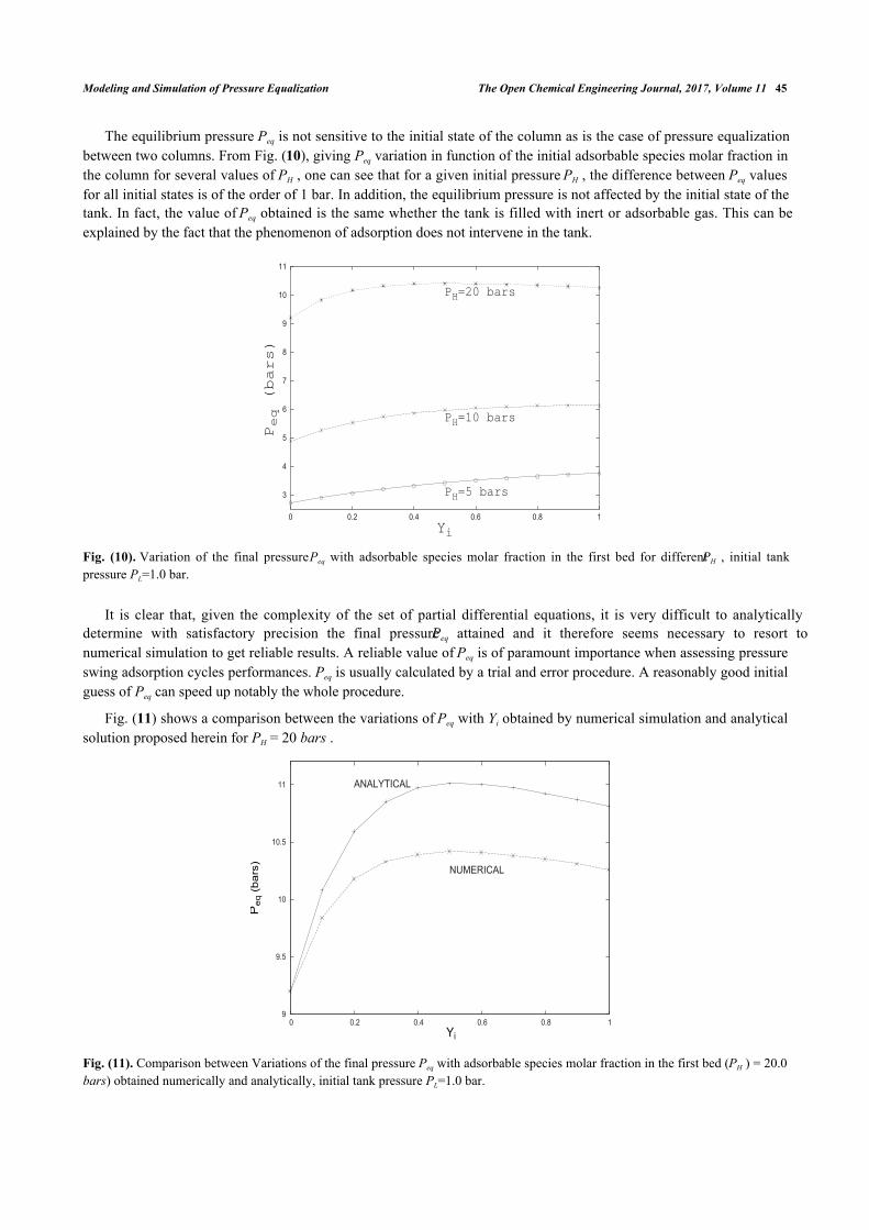
The equilibrium pressure Peq is not sensitive to the initial state of the column as is the case of pressure equalizationbetween two columns. From Fig. (10), giving Peq variation in function of the initial adsorbable species molar fraction inthe column for several values of PH , one can see that for a given initial pressure PH , the difference between Peq valuesfor all initial states is of the order of 1 bar. In addition, the equilibrium pressure is not affected by the initial state of thetank. In fact, the value of Peq obtained is the same whether the tank is filled with inert or adsorbable gas. This can beexplained by the fact that the phenomenon of adsorption does not intervene in the tank.

Fig. (10). Variation of the final pressure Peq with adsorbable species molar fraction in the first bed for different PH , initial tankpressure PL=1.0 bar.

It is clear that, given the complexity of the set of partial differential equations, it is very difficult to analyticallydetermine with satisfactory precision the final pressure Peq attained and it therefore seems necessary to resort tonumerical simulation to get reliable results. A reliable value of Peq is of paramount importance when assessing pressureswing adsorption cycles performances. Peq is usually calculated by a trial and error procedure. A reasonably good initialguess of Peq can speed up notably the whole procedure.

Fig. (11) shows a comparison between the variations of Peq with Yi obtained by numerical simulation and analyticalsolution proposed herein for PH = 20 bars .

Fig. (11). Comparison between Variations of the final pressure Peq with adsorbable species molar fraction in the first bed (PH ) = 20.0bars) obtained numerically and analytically, initial tank pressure PL=1.0 bar.

3

4

5

6

7

8

9

10

11

0 0.2 0.4 0.6 0.8 1

Peq (bars)

Yi

PH=20 bars

PH=10 bars

PH=5 bars

9

9.5

10

10.5

11

0 0.2 0.4 0.6 0.8 1

Peq

(ba

rs)

Yi

NUMERICAL

ANALYTICAL


It is interesting to note that both solutions provide the same trend of evolution of Peq with Yi. In both cases, theequilibrium pressure increases initially with Yi to attain a maximum value and then begins a slight decrease. Thedifference between the two solutions does not exceed 0.5 bar despite the rough approximations considered for theanalytical solution. The value of Peq given by the analytical solution is always greater than the one given by thenumerical solution. For Yi = 0 (the column contains only an inert gas), note the coincidence of the numerical value of Peq

with that obtained analytically (from equations 17 or 18). One can often resort to comparison between numerical andanalytical solutions in special cases to prove the reliability of modelling and numerical resolution. It is the case herein.

Fig. (12). Experimental evolution with time of the pressure at the closed end of the column during equalization for various values ofPH , the arrow indicates increasing values of PH ,PL = 1.0 bar, L = 1 m, Dcol=5 cm.

Fig. (13). Experimental evolution with time of the pressure inside the tank during equalization for various values of PH , the arrowindicates increasing values of PH ,PL = 1.0 bar, L = 1 m, Dcol=5 cm.

5

10

15

20

0 0.5 1 1.5 2 2.5 3 3.5 4

P(B

AR

S)

t(s)

1

2

3

4

5

6

7

8

9

10

0 0.5 1 1.5 2 2.5 3 3.5 4

P(B

AR

S)

t(s)


To validate the simulation results, many pressure equalization experiments have been carried out and compared tosimulations. Figs. (12 and 13) show the experimental variation with time of pressure at the closed end of the columnand inside the tank during equalization respectively for many different initial values of PH (between 2 and 20 bars withan increment of 2 bars). The initial pressure prevailing in the tank is always PL=1 bar. The column and the tank containinitially pure hydrogen. For the latter experiments, the tank is an empty column having the same length and diameter asthe packed one (D=0.05 m, L=1 m). The arrow indicates direction of increasing initial PH value. Pressure at the closedend of the bed decreases while the pressure in the tank increases during equalization until reaching the equilibriumpressure. For the different experiements, the value of Peq obtained is very close to the one given by the equation (17)which is valid for a non adsorbable gas. Fig. (14) gives a comparison between time change of pressure at the closed endof the column obtained both experimentally and numerically. It can be seen that the simulation allows to model theexperimental results in a satisfactory way. The slight difference that can be noticed is due to the fact that the volume oftubings relating the column and the tank is not taken into account in modeling. This is why the value of equilibriumpressure obtained by simulation is slightly greater than the experimental one. The same remarks are valid for timevariation of pressure in the tank.

Fig. (14). Evolution with time of the pressure at the closed end of the column during equalization: Comparison between experimentalresults and simulation for various values of PH (20, 16, 10 and 6 bars), PH = 10.0 bars, PL = 1.0 bar, L = 1 m, Dcol =5 cm.

Let us now compare numerical and experimental results when the packed bed initially contains a binary gas, one ofwhich is adsorbable (methane). Fig. (15) shows the experimental change with time of pressure at the closed end of thecolumn and inside the tank during equalization for many initial states of the column. In fact, prior to pressureequalization, the column is in equilibrium with different binary mixtures of H2 and CH4 (for yCH4 = 0, 0.1, 0.2 and 1.0) at PH =10 bars whereas the tank is filled with H2 at PL=1 bar.

The arrow indicates direction of increasing initial methane molar fraction in the column. The end of the equalizationstep is obtained when the pressures in the bed and the tank become equal. It can be seen that the equalization time teq,corresponding to obtaining the same pressure in the column and the tank, increases with CH4 molar fraction. Thehighest and lowest values of teq are obtained for columns which have been initially in equilibrium with pure methaneand pure H2 respectively. The experimental value of Peq obtained when connecting a column initially saturated with pureCH4 with the tank is Peq =6.56 bars, this value is not far from Peq = 6.47 bars given by simulation, but very far from Peq

=4.88 bars if equation (17) is used.

5

10

15

20

0 1 2 3 4 5 6 7

P(B

AR

S)

t(s)

EXPERIMENTAL DATASIMULATION


Fig. (15). Evolution with time of the pressure at the closed end of the column and inside the tank during equalization for many initialstates of the column Yi (0, 0.1, 0.2 1.0), the arrow indicates increasing values of Yi , PL = 1.0 bar, L = 1 m, Dcol = 5 cm.

Fig. (16) gives a comparison between the values of the equilibrium pressure Peq obtained experimentally,numerically and analytically (from equation (14)). The values of PH and PL are 10 bars and 1 bar respectively. Theinitial methane molar fraction in the packed bed varies from 0 to 1. The experimental values are slightly underestimatedby the numerical values and slightly overestimated by the analytical values. Indeed, the maximum difference does notexceed 0.1 bar when comparison is made with the experimental values. For the experiment with a column containinginitially pure hydrogen (yCH4 =0), the experimental value of Peq obtained is 4.8 bars whereas the value given both bysimulation and analytical solution is 4.88 bars. As previously mentioned, this slight difference is attributed to the fact ofneglecting the volume of tubings connecting the packed bed and the tank. Indeed, the minimum value can not be lowerthan 4.88 bar obtained by the analytical solution (equation (22)) for a column containing only an inert gas or bysimulation for the same case. The sole source of the discrepancies is to be attributed to the impact of the tubing volume.It is highly unlikely that the accuracy of the pressure measuring instrument is the cause of this deviation insofar as thevalue of the equilibrium pressure is obtained both by a manometer (pressure gauge) installed on the column (observablevisually) and by a pressure transducer (electrical signal), the two values obtained are identical.

Fig. (16). Comparison between the values of Peq obtained experimentally, numeri-cally and analytically for various values of theadsorbable species molar fraction in the first bed, PH = 10.0 bars, PL = 1.0 bar, L = 1 m, Dcol = 5 cm.

0

2

4

6

8

10

0 2 4 6 8 10 12 14

P(B

AR

S)

t(s)

Initial mole fraction in the bed 0%

10%20%

100%

5

5.5

6

6.5

0 0.2 0.4 0.6 0.8 1

Peq

(ba

rs)

Yi

ANALYTICALEXPERIMENTAL

NUMERICAL


Fig. (17) shows a comparison between the values of the methane molar fraction Yeq in the tank at the end of theequalization step obtained experimentally, numerically and analytically (from equation (16)). It has to be mentioned thatthe experimental value of methane molar fraction in the tank is obtained by averaging the values for five samples of gasrecovered from the tank after disconnecting it from the packed bed. The gas analysis is done by infrared absorptionspectroscopy. The experimental values are close to the ones obtained by numerical simulation.The values given by theanalytical solution are somewhat less precise, for example, the values obtained experimentally, numerically andanalytically are 0.82, 0.84 and 0.91 respectively for the case of a bed initially saturated with pure methane (yCH4 =1).Hence, the numerical simulation of the equalization step is very satisfactory and allows to obtain reliable results eitherfor the equilibrium pressure or mole fraction in the tank. The analytical solution gives acceptable results despite thesimplifying assumptions considered, it permits to assess rapidly Peq and Yeq without the need to resort to a cubersomemodeling.

Fig. (17). Comparison between the values of Yeq obtained experimentally, numerically and analytically for various values of theadsorbable species molar fraction in the first bed, PH = 10.0 bars, PL = 1.0 bar, L = 1 m, Dcol = 5 cm.

One of parameters, among others, which contributes enormously to the optimization of the operation of pressureequalization is the tank volume Vtank . It should be borne in mind that the goals of this step are to maximize the pureproduct transfer from the column to the tank for increasing product recovery and to conserve mechanical energy.

In both cases, it is important that the adsorbable species molar fraction of the gas transferred to the tank at the end ofpressure equalization is as low as possible. This would allow a better partial purge if the tank gas is used to partiallypurge a column just after the depressurization step, on one hand, and the preservation of the capacity of the adsorptioncolumn if the tank gas is used to pressurize a column at the end of a low pressure purge step on the other hand. It thenbecomes important to optimize the pressure equalization step so that the gas transferred from the column to the tank isminimally contaminated by the adsorbable species.

Fig. (18) shows the variation of Peq in function of the tank volume. The equilibrium pressure Peq decreases notablywith Vtank . Thus, as an example, Peq =4.75 bars for Vtank =5.0Vcol and Peq =13.8 bars for Vtank =0.5 Vcol. It follows thatincreasing the volume of the tank presents the disadvantage of lowering enormously pressure. If the gas collected in thetank is intended for a column pressurization, one will have to choose the right volume of the tank so as to reach thedesired pressure in the column to be pressurized at the end of the equalization step.

0

0.2

0.4

0.6

0.8

1

0 0.2 0.4 0.6 0.8 1

Yeq

Yi

ANALYTICALEXPERIMENTAL

NUMERICAL


Fig. (18). Variation of the final pressure Peq with the ratio Vtank /Vcol, initial state: Bed (Yi = 0.5, PH = 20.0 bars), tank (Yi = 0.0, PL = 1.0bar).

CONCLUSION

It is issential to pay a great attention when choosing models to simulate pressure swing processes. The pressureequalization step must be treated with special care since its impact on the assessment of the overall performance of theprocess is notable. If the equilibrium pressure is not accurately evaluated, this could lead inevitably to erroneoussimulations in the case where the PSA cycle comprises a pressure equalization step. In fact, if rough approximations areconsidered, estimated Peq may differ from the real value leading to inaccurate simulation results. The analytical solutionproposed herein for assessing the final pressure when connecting a bed and an empty tank could be consideredacceptable despite the simplifying assumptions considered. Based on the comparisons presented, one can conclude thatthe agreement between the experimental and numerical results relative to the equilibrium pressure and the equilibriummole fraction of the adsorbable species in the tank is very satisfactory, thus simulation results could be consideredreliable and used safely so as to optimize PSA cycles. If the gas transferred to the tank is destined for subsequentcolumn pressurization, the choice of the tank volume will depend on the value of the desired pressure to be reached inthe column to be pressurized at the end of the equalization step.

NOMENCLATURE

b = parameter of Langmuir isotherm, P a−1

C = bulk phase concentration, mol/m3

cp = heat capacity, J /(molK) or J/(kgK)

cp = mean intra-particle gas phase concentration, mol/m3

Dax = mass axial dispersion coefficient, m2/s

Dcol = column diameter, m dp : Particle diameter, m

Dp = pore diffusivity, m2/s

Ds = surface diffusivity, m2/s

h = heat transfer coefficient, W /(m2s)

H = enthalpy, J /mol L: Bed length, m

Ng = number of species in the gas mixture

4

6

8

12

14

16

18

20

0 1 2 3 4 5

Peq(bars)

Vtank

/Vcol


P = total pressure, P a

Q = molar flow rate, mol/s

Qm = parameter of Langmuir isotherm, mol/kg

q = adsorbed phase concentration, mol/m3 or mol/kg

R = gas constant or particle radius, J /(molK) or m

S = cross section of the column, m2

u = interstitial velocity, m/s

U = internal energy, J /mol

V = volume, m3

T = temperature, K t: Time, s

Z = compressibility factor of the gas mixture

z = axial coordinate in the bed, m

GREEK LETTERS

∆H = heat of adsorption, J /mol

ϵ = interparticle porosity

ϵp = intraparticle porosity

ϵt = total porosity

µ = fluid viscosity, kg/(m s)

ρ = fluid or bed density, kg/m3

τ = particle tortuosity factor

SUPERSCRIPTS∗ = equilibrium

i = refers to species i

SUBSCRIPTS

a = refers to adsorbed phase

A = refers to the adsorbable species

b = refers to the bed

col = refers to column

e = refers to surroundings

eq = refers to the equilibrium state

f eed = at the bed entrance

g = refers to gas phase

H = refers to the high value

i = refers to species i

I = refers to the inert

L = refers to the low value

out = at the bed exit

p = refers to adsorbent particle

s = refers to solid phase

tank = refers to tank

0 = initial condition

CONSENT FOR PUBLICATION

Not applicable.


CONFLICT OF INTEREST

The authors declare no conflict of interest, financial or otherwise.

ACKNOWLEDGEMENTS

Declared none.

REFERENCES

[1] N.H. Berlin, U.S. Paten, vol. 280, no. 3, p. 536, 1966. [to Exxon Research and Engineering.].

[2] R. Banerjee, K.G. Narayankhedkar, and S.P. Sukhatme, "Exergy analysis of pressure swing adsorption processes for air separation", Chem.Eng. Sci., vol. 45, no. 2, pp. 467-475, 1990.[http://dx.doi.org/10.1016/0009-2509(90)87033-O]

[3] A. Bossy, and D. Tondeur, "A non-linear equilibrium analysis of blowdown policy in pressure swing adsorption separation", Chem. Eng. J.,vol. 48, pp. 173-182, 1992.[http://dx.doi.org/10.1016/0300-9467(92)80033-7]

[4] A.S. Chiang, "An analytical solution to equilibrium PSA cycles", Chem. Eng. Sci., vol. 51, no. 2, pp. 207-216, 1996.[http://dx.doi.org/10.1016/0009-2509(95)00267-7]

[5] O.J. Smith, and A.W. Westerberg, "The optimal design of pressure swing adsorption systems", Chem. Eng. Sci., vol. 46, no. 12, pp.2967-2976, 1991.[http://dx.doi.org/10.1016/0009-2509(91)85001-E]

[6] K. Warmuzinski, "Effect of pressure equalization on power requirements in PSA systems", Chem. Eng. Sci., vol. 57, pp. 1475-1478, 2002.[http://dx.doi.org/10.1016/S0009-2509(02)00060-X]

[7] K. Warmuzinski, and M. Tanczyk, "Calculation of the equalization pressure in PSA systems", Chem. Eng. Sci., vol. 58, pp. 3285-3289, 2003.[http://dx.doi.org/10.1016/S0009-2509(03)00170-2]

[8] J.A. Delgado, and A.E. Rodrigues, "Analysis of the boundary conditions for the simulation of the pressure equalization step PSA cycles",Chem. Eng. Sci., vol. 63, pp. 4452-4463, 2008.[http://dx.doi.org/10.1016/j.ces.2008.06.016]

[9] Chahbani M.H., and D. Tondeur, "Predicting the final pressure in the equalization step of PSA cycles", Sep. Pur. Technol., vol. 71, pp.225-232.

[10] M. Yavary, H. Ale-Ebrahim, and C. Falamaki, "The effect of number of pressure equalization steps on the performance of pressure swingadsorption process", Chem. Eng. Prog., vol. 87, pp. 35-44, 2015.[http://dx.doi.org/10.1016/j.cep.2014.11.003]

[11] W.D. Marsh, R.C. Hoke, F.S. Pramuk, and C.W. Skarstrom, "Pressure equalization depressuring in heallen adsorption", U.S. Patent, vol. 3,pp.142-547, July 28, 1964.

[12] M. Yavary, H. Ale-Ebrahim, and C. Falamaki, "The effect of reliable prediction of final pressure during pressure equalization steps on theperformance of PSA cycles", Chem. Eng. Sci., vol. 66, pp. 2587-2595, 2011.[http://dx.doi.org/10.1016/j.ces.2011.03.005]

[13] D. Tondeur, and C. Wankat Phillip, "Gas Purification by Pressure Swing Ad- sorption", Separ. Purif. Rev., vol. 14, no. 2, pp. 157-212, 1985.[http://dx.doi.org/10.1080/03602548508068420]

[14] L.R. Petzold, A Description of DASSL: a Differential / Algebraic System Solver., Sandia National Laboratories: Livermore, California, 1982.

[15] Chahbani M.H., "Separation de gaz par adsorption modulee en pression", PhD thesis, ENSIC, INPL, France, 1996.

[16] E. Alpay, C.N. Kenney, and D.M. Scott, "Simulation of rapid pressure swing adsorption and reaction processes", Chem. Eng. Sci., vol. 48, no.18, pp. 3173-3186, 1993.[http://dx.doi.org/10.1016/0009-2509(93)80203-3]

[17] J.M. Prausnitz, R.C. Reid, and B.E. Poling, The Properties of Gases and Liquids., McGraw-Hill: New York, 1987.

© 2017 Chahbani et al.

This is an open access article distributed under the terms of the Creative Commons Attribution 4.0 International Public License (CC-BY 4.0), acopy of which is available at: https://creativecommons.org/licenses/by/4.0/legalcode. This license permits unrestricted use, distribution, andreproduction in any medium, provided the original author and source are credited.

http://dx.doi.org/10.1016/0009-2509(90)87033-O

http://dx.doi.org/10.1016/0300-9467(92)80033-7

http://dx.doi.org/10.1016/0009-2509(95)00267-7

http://dx.doi.org/10.1016/0009-2509(91)85001-E

http://dx.doi.org/10.1016/S0009-2509(02)00060-X

http://dx.doi.org/10.1016/S0009-2509(03)00170-2

http://dx.doi.org/10.1016/j.ces.2008.06.016

http://dx.doi.org/10.1016/j.cep.2014.11.003

http://dx.doi.org/10.1016/j.ces.2011.03.005

http://dx.doi.org/10.1080/03602548508068420

http://dx.doi.org/10.1016/0009-2509(93)80203-3

https://creativecommons.org/licenses/by/4.0/legalcode

the open chemical engineering journal€¦ · · 2017-11-09the open chemical engineering journal,...

Documents