1

A review of modelling tools for implementation of the EU

Water Framework Directive in handling diffuse water

pollution

Y.S. Yang, L. Wang*

______________________________________________________________________

ABSTRACT

A numerical catchment-scale model capable of simulating diffuse water pollution is

necessary in sustainable environmental management for better implementation of the

EU Water Framework Directive. This paper provides critical reviews of most popular

and free models for diffuse water modelling, with detailed sources and application

potential. Based upon these reviews, further work of selecting and testing the HSPF

model was carried out, with a case study in the Upper Bann Catchment, Northern

Ireland. The calibrated and validated HSPF model can well represent the characteristics

of surface water quantity and quality. Climate change scenario evaluation in five years

showed that when the annual mean temperature increase 3°C the mean yearly total

runoff volume will decrease by 11.1% and the mean daily river flow 11.4%. If 20%

crop and pasture land is converted into forest land in the study area, the mean river

concentration of nitrate, nitrite, NH4 and PO4 in five years will decrease by 19.4%,

33.3%, 31.3% and 31.3% respectively. When applying filter strip method in 80% crop

and pasture land in the area, the reduction of the mean concentration of nitrate, nitrite,

NH4 and PO4 in five years will be 15.3%, 33.3%, 31.3%, and 5.6% respectively. This

* Y.S. Yang

Cardiff University, School of Earth and Ocean Sciences, Cardiff CF10 3YE, UK

L. Wang

British Geologic Survey, Keyworth, Nottingham NG12 5GG, UK.

e-mail: Lei.Wang@bgs.ac.uk

2

study shows that HSPF is a suitable model in handling diffuse source water pollution,

which can be introduced into the Programme of Measures in the River Basin

Management Plans for better implementation of the EU WFD.

Keywords: Diffuse water pollution; water quality modelling; Catchment; EU Water

Framework Directive; Climate change.

Software availability

Software name/source: all reviewed software are mentioned in the text.

1. Introduction

Water pollution, a global problem, is not only an environmental issue but also an

economic and human health problem. As a part of a substantial restructuring of EU

water policy and legislation, the EU Water Framework Directive (WFD) was agreed by

the European Parliament and Council in September 2000 and came into force on 22nd

December 2000 (EC, 2000). The EU WFD sets a framework for comprehensive

management of water resources in the European Community, within a common

approach and with common objectives, principles and basic measures. The fundamental

objectives of the Water Framework Directive are to maintain a ―high status‖ of inland

surface waters, estuarine and coastal waters and groundwater where it exists, prevent

any deterioration in the existing status of waters and achieve at least a ―good status‖ in

relation to all waters by 2015 (Heinz et al., 2007; Krause et al., 2007). Member States

will have to ensure that a coordinated approach for water management is adopted for the

achievement of the objectives of the WFD and for implementation of acting

programmes for the purposes (Borowski et al., 2007; De-Kok et al., 2009).

Diffuse water pollution (DWP) has been realised as a major threat for water quality

and the biggest remaining problem of water pollution in many countries (Campbell et al.,

2004; Gaddis et al., 2007; Orr et al., 2007; Hessea et al., 2008). DWP is also the main

3

threat for meeting the requirement of the EU WFD (DoE and DARD UK, 2003; Ferrier

et al., 2004; Torrecilla et al., 2005; Silgram et al., 2008). The serious problem for

implementation of the EU WFD is lack of pragmatic methods and tools to fulfil new

tasks from the EU WFD for most EU Member States (Mostert, 2003; Giupponi, 2005;

Heinz et al., 2007). The scientific measures or tools that can actually be used or

developed for implementation of the EU WFD, especially in handling DWP, are still

largely unknown to the EU Member States (UK EA, 2005; Krause et al., 2007).

Not all water quality problems require a water quality modelling effort. Numerical

water modelling, however, is necessary for the sustainable DWP management at

catchment scale. Compared to point pollution, DWP is more complex and difficult to

control due to its numerous and dispersed sources, and the difficulties in tracing its

pathways (Wang and Yang, 2008). Suitable numerical DWP models not only provide

quantitative description of water quantity and quality to the temporal and spatial details

and the contaminant fate and transport in the DWP phases of source – pathway – target,

varying greatly with different natural and landuse conditions; but also are capable of

evaluating the impacts of the management plans on water processes in which the

extension and extrapolation of measured data are needed (Van-Ast et al., 2005; Galbiati

et al., 2006; Even et al., 2007). The quality and complexity of the DWP models will

directly affect the reliability of modelling results. The good DWP models should

consider these factors: weather-driven processes and meteorological conditions (e.g.

precipitation, air temperature, solar radiation, and wind speed) obviously influencing the

water quantity and quality; various diffuse source parameters including pesticides,

nutrients, sediments from eroded or overgrazed lands, and microorganisms; complicated

soil-water interfaces for water flow and solute fluxes considering natural and human

activities (Krause et al., 2007; Collins and McGonigle, 2008). Human activities related

to land uses, such as farming, urbanisation and waste water disposals can produce great

impact on the status of waters by modifying soil property and structure, changing

nutrient chemical process in soil and bringing in pollution loads. In reality a catchment

contains not only pervious agricultural land but also impervious urban land; it is

4

important that the DWP models are capable of evaluating the effectiveness of proposed

strategies to reduce the loading of agricultural or other contaminants into water course

under the climate change – an inevitable global problem that we have to face. Therefore,

the factors of application scale, contaminant simulation capability, nutrient cycling

processes in soil, climate change response, pervious and impervious shallow geology,

land use supporting, etc., should be considered in choosing a numerical catchment water

modelling tool for better implementation of the EU WFD in handling DWP. Some

modelling comparison literatures can be found, for example Nasr et al. (2007) studied

phosphorus export modelling at catchment scale; majority of work was done about

specific modelling effort from various, diverse models for various DWP issues from

agricultural nutrient loading, coastal water quality assessment (Yuan et al., 2007;

Krause et al., 2008), to detailed contribution from root system and large scale

transboundary modelling (Diogo et al., 2008; Sohier et al., 2009).

This paper aims to 1) critically review the popular water models in selecting a

proper numerical tool for better implementation of the EU WFD in modelling DWP; 2)

assess a selected model – Hydrological Simulation Program – FORTRAN (HSPF) by

applying it in water quantity and nutrient quality modelling; 3) present a case study with

HSPF model in the Upper Bann Catchment, Northern Ireland; and 4) evaluate the

impact of DWP management strategies on water quality.

2. Critical review for model selection

The choice of the numerical model depends on the objectives of the study. For better

implementation of the EU WFD in the DWP field, water modelling should be able to: 1)

get reliable water quantity and quality simulation results; 2) be applied at

catchment/watershed scale or larger scale; 3) calculate the complex nutrient biochemical

process in different soil types; 4) take into account both diffuse and point source

pollutions; 5) model the DWP process from both agriculture and urban land uses; and 6)

evaluate the impact of climate change scenarios on water and its quality.

5

It was the 1970's and early 1980's when people realised increasing water pollution

problems. The DWP issue has been a headache since then and scientists have been

developing and updating mathematical models to characterise the pollutant loadings and

water quality impacts, and more and more water simulation models have been available.

Models below are the most notable, well known, operational and free models.

2.1. Model description

Chemicals, Runoff, and Erosion from Agricultural Management Systems (CREAMS)

(Knisel, 1980), a field scale model, was developed by the US Department of Agriculture

(USDA) - Agricultural Research Service (ARS) for the analysis of agricultural best

management practices (BMP) for pollution control. The model can be obtained from the

website http://www.wiz.uni-kassel.de/model_db/mdb/creams.html. This model uses

separate hydrology, erosion, and chemistry sub-models connected together to calculate

runoff volume, peak flow, infiltration, evapotranspiration, soil water content, and

percolation on a daily basis; simulate plant nutrients and pesticides; and determine

storm load, average concentrations of sediment-associated and dissolved chemicals in

the runoff, sediment, and percolation through the root zone (Leonard and Knisel, 1984).

User defined management activities, such as aerial spraying, soil incorporation of

pesticides, animal waste management, and agricultural best management practices

(minimum tillage, terracing, etc.), can be simulated by CREAMS. Groundwater

Loading Effects of Agricultural Management Systems (GLEAMS) was developed by

the USDA - ARS (Leonard et al., 1987) based on CREAMS. GLEAMS, consisting of

three major components namely hydrology, erosion/sediment yield, and pesticides, can

be treated as the vadose zone component of the CREAMS model. The soil is divided

into various layers, with a minimum of 3 and a maximum of 12 layers of variable

thickness are used for water and pesticide routing (Knisel et al., 1989). The limitations

of CREAMS/GLEAMS include: 1) the maximum size of the simulated area is limited to

a small field plot; 2) they are limited in data management and handling; 3) they can not

simulate instream processes; 4) they have limited simulation capability for snow

6

accumulation, melt, and resulting runoff, and hydrologic impacts of frozen ground

conditions (Kauppi, 1982; Knisel et al., 1983).

Storm Water Management Model (SWMM) was developed for US EPA as a single-

event model specifically for the analysis of combined sewer overflows (CSO) (Metcalf

and Eddy Inc. et al., 1971; Roesner et al., 1988). The model is available at http://

www.epa.gov/ednnrmrl/models/swmm/index.htm. SWMM consists of several modules,

namely Runoff, Transport and Extran, designed to simulate both continuous and single

event quantity and quality processes in the urban hydrologic cycle. Storm sewers,

combined sewers, and natural drainage systems can be simulated. Storage, Treatment,

Overflow, Runoff Model (STORM) was developed by the Corps of Engineers

Hydrologic Engineering Center of US for the application of the San Francisco master

plan for CSO pollution abatement (HEC, 1977). STORM contains simplified hydrologic

and water quality routines for continuous simulation in urban areas, and can be used to

calculate hourly runoff volumes and depths, snowmelt, dry-weather flows, suspended

solids, settleable solids, BOD, total coliforms, ortho-phosphate, and nitrogen. The

weaknesses of SWMM and STORM include that they both are urban models; the

quality simulation of SWMM is weak in the representation of the true physical,

chemical and biological processes that occur in the nature; SWMM has weak

groundwater simulation capability; STORM uses the quality routines embodied in

SWMM with very few modifications; although STORM has less data requirements its

hydrologic routines are too simple for complicated water simulation (Donigan and

Huber, 1991; Shoemaker et al., 2005).

Areal Nonpoint Source Watershed Environment Response Simulation (ANSWERS)

was developed by the Agricultural Engineering Department of Purdue University

(Beasley and Huggins, 1981). It is available from

http://cobweb.ecn.purdue.edu/~aggrass/models/ answers/. The ANSWERS model is

capable of predicting the hydrologic and erosion response of agricultural watersheds.

Since it is a distributed parameter model, its application requires that the watershed to

be subdivided into a grid of square elements. The modular program structure of

7

ANSWERS allows easier modification and customising of existing program code.

However, there are limitations for ANSWERS: 1) although it has a PC version for small

watershed application, a mainframe computer is required for a simulation run of

ANSWERS on a large watershed; 2) this storm event model requires complex input data

preparation; 3) the water quality constituents modelled are limited to nitrogen and

phosphorous, and snowmelt processes or pesticides cannot be simulated; 4) nitrogen and

phosphorus are simulated using correlation relationships between chemical

concentrations, sediment yield and runoff volume, and no transformation of nitrogen

and phosphorus is considered (Donigan and Huber, 1991).

Unified Transport Model for Toxic Materials (UTM-TOX) was developed by Oak

Ridge National Laboratory for the U.S. EPA Office of Pesticides and Toxic Substances,

Washington, D.C. (Patterson et al., 1983). UTM-TOX includes atmospheric transport,

terrestrial ecology and hydrology and Wisconsin hydrologic transport model to establish

chemical mass balances, make chemical budgets and to estimate chemical

concentrations in the environment. The limitations of this model are that it 1) ignores

the interaction between chemicals and sediment in streams; 2) is quite complex and

requires significant user expertise; 3) concentrates on pesticides and toxic substances

only.

Pesticide Root Zone Model (PRZM) was developed at the U.S. EPA Environmental

Research Laboratory in Athens, Georgia (Carsel et al., 1984), which is available at

http:// www.epa.gov/ceampubl/gwater/przm3/index.htm. PRZM can be used to simulate

chemical movement in unsaturated zone within and immediately below the plant root

zone using of its hydrology and chemical transport modules. The most recent version of

PRZM is included in an integrated root/vadose/groundwater model called RUSTIC

(Risk of Unsaturated/Saturated Transport and Transformation of Chemical

Concentrations) for the prediction of pesticide fate and transport through the crop root

zone, and saturated zone to drinking water wells (Dean et al., 1989). PRZM can not

handle lateral flow because of its 1D capability in the vertical direction; PRZM only

simulates downward water movement and does not account for diffusive movement due

8

to soil water gradients; the model only simulates organic chemicals, for example

pesticides.

Agricultural Nonpoint Source Pollution Model (AGNPS) was developed by USDA -

ARS (Young et al., 1986) and is available from http://www.wsi.nrcs.usda.gov/products/

w2q/h&h/tools_models/agnps/index.html. It is a distributed parameter model, and can

be used to estimate nutrients and sediments in runoff, and to compare the effects of

various pollution control practices in watershed management. AGNPS can also handle

point source pollutions. The methods used for the prediction of nitrogen and phosphorus

yields from the watershed are also used in CREAMS. The methods for nitrogen and

phosphorus concentration calculations are similar to ANSWERS. The limitations of

AGNPS include: 1) the model does not handle pesticides; 2) the pollutant transport

component needs further field testing; 3) nutrient transformation and instream processes

are not within model capabilities; 4) it is used only to simulate single event; 5) it is an

empirical model; 6) channels are assumed to have a triangular shape (Donigan and

Huber, 1991; Shoemaker et al., 2005).

Enhanced Stream Water Quality (QUAL2E) model, a comprehensive and versatile

1D stream water quality steady model, was developed based on Streeter-Phelps model

(Streeter and Phelps, 1925) to simulate nutrient dynamics, algal production, and

dissolved oxygen with the impact of benthic and carbonaceous demand in streams

(Brown and Barnwell, 1987). The model is available at http://

www.epa.gov/athens/wwqtsc/html /qual2k.html. Fifteen water quality variables are

modelled in QUAL2E. The model is intended as a waste load allocation and water

quality planning tool for developing total maximum daily loads (TMDL). It can also be

used in conjunction with field sampling for identifying the magnitude and quality

characteristics of nonpoint sources. The limitations of QUAL2E include: 1) 1D channel

that cannot handle tidal impact; 2) steady flow is not able to model variable flow

condition; 3) the model is unsuitable for rivers that experience temporal variations in

streamflow or where the major discharges fluctuate significantly over a diurnal or

shorter time period (Birgand, 2004).

9

Simulator for Water Resources in Rural Basins (SWRRB) was developed by

modifying CREAMS for evaluating basin scale water quality by daily simulation of

weather, hydrology, crop growth, sedimentation, nitrogen, phosphorous and pesticide

movement (Williams et al., 1985). It‘s available at http://rhino.cee.odu.edu/model/

swrrbwq.php. The model considers both soluble pollutants and sediment attached

pollutants. The nitrogen and phosphorus calculations are performed using relationships

between chemical concentration, sediment yield and runoff volume. However in

SWRRB, there is very minimal model documentation; the snow accumulation processes

are ignored in the hydrology component; no comprehensive instream simulation is

available for pesticides calculation; nutrient transformations along with pesticide

daughter products are not accounted for in the model (Arnold et al., 1989).

Soil Water and Analysis Tools (SWAT), a physical-based model, was developed by

USDA-ARS in the early 1990s for the prediction of the long-term impact of rural and

agricultural management practices (such as detailed agricultural land planting, tillage,

irrigation, fertilisation, grazing, and harvesting procedures) on water, sediment and

agricultural chemical yields in large, complex watersheds with varying soils, land use,

and management conditions (Arnold et al., 1998). It can be downloaded free from

http://www.brc.tamus.edu/swat/. SWAT incorporates features of several ARS models

and is a direct outgrowth of the SWRRB and CREAMS model. Since SWAT is a

physically based model, watersheds with no monitoring data can be modelled; the

relative impact of alternative input data (such as changes in management practices,

climate, vegetation) on water quality or other variables of interest can be quantified

using readily available inputs. While SWAT can be used to study more specialised

processes such as bacteria transport, the minimum data required to make a run are

commonly available from government agencies. In addition, the continuous time SWAT

model enables users to study long-term impacts. However, SWAT has some limitations:

1) not for simulating sub-daily events such as a single storm event and diurnal changes

of dissolved oxygen in a water body; 2) only route one pesticide each time through the

stream network; 3) can not specify actual areas to apply fertilisers; 4) a large watershed

10

can be divided into hundreds of hydrologic response units (HRU) resulting in many

hundreds of input files, which are difficult to manage and modify without a solid

interface; 5) the parameters of the equations are not directly measured by using data; 6)

it has the difficulty in simulating snowmelt; 7) it does not simulate detailed event based

flood and sediment routing; 8) it has difficulties in modelling floodplain erosion and

snowmelt erosion during the spring and winter months (Peterson and Hamlett 1998;

Benaman et al., 2005; Shoemaker et al., 2005). Although efforts have been made to

incorporate more process-based equations, some of the basic processes modelled by

SWAT still have room for improvement.

The SHETRAN system was developed by the Water Resources Systems Research

Laboratory (WRSRL) based on the SHE (Système Hydrologique Européen) through the

international collaboration between groups in the UK, Denmark, and France (Ewen,

1995). SHETRAN is a 3D, surface/subsurface, physically-based, spatially-distributed

and finite-difference model for water flow, multifraction sediment transport and

multiple, reactive solute transport in river basins. It gives a detailed description in time

and space of the flow and transport in the basin, which can be visualised using animated

graphical computer displays. SHETRAN represents physical processes using physical

laws applied on a 3D finite-difference mesh to model the hourly flow and transport for

periods of up to a few decades. Since SHETRAN is a new model, its limitations need to

be discussed in future worldwide applications.

Hydrological Simulation Program – FORTRAN was developed by US

Environmental Protection Agency (USEPA) to represent contributions of sediment,

nutrients, pesticides, conservatives and faecal coliforms from agricultural areas; and to

continuously simulate water quantity and quality processes on pervious and impervious

land surfaces and in streams and well-mixed impoundments (Barnwell and Johanson,

1981). Details are available at http://www.epa.gov/ceampubl/swater/hspf/index.htm. By

supporting conventional and toxic organic pollutants from both point sources and

diffuse sources, HSPF is one of few comprehensive watershed hydrology and water

quality models that allow the integrated simulation of land and soil contaminant runoff

11

processes with instream hydraulic, water temperature, sediment transport, nutrients, and

sediment-chemical interactions (Gallagher and Doherty, 2007; Ribarova et al., 2008).

The runoff flow rate, sediment load (sand, silt, and clay), nutrient and pesticide

concentrations, and historical time series of water quantity and quality at any point in a

watershed can be calculated using this model (Tzoraki and Nikolaidis, 2007; Choi and

Deal, 2008). The runoff quality capabilities include both simple relationships (e.g.

empirical buildup/washoff and constant concentrations) and detailed soil process

options (e.g. leaching, sorption, soil attenuation, and soil nutrient transformations).

HSPF includes organic chemical transfer and reaction processes of hydrolysis, oxidation,

photolysis, biodegradation, a volatilization, and sorption. The instream nutrient

processes include DO, BOD, nitrogen and phosphorus reactions, pH, phytoplankton,

zooplankton, and benthic algae (Tzoraki and Nikolaidis, 2007). Any time step from 1

minute to 1 day can be used, and any period from a few minutes to hundreds of years

may be simulated. HSPF is generally used to assess the effects of land-use change,

reservoir operations, point or diffuse source treatment alternatives, flow diversions, etc

(Choi and Deal, 2008; Cho et al., 2009). The limitations of HSPF include 1) it relies on

many empirical relationships to represent physical processes; 2) its lump simulation

processes for each land use type at the sub-watershed does not consider the spatial

distribution of one land parcel relative to another in the watershed; 3) it approaches a

distributed model when smaller sub-watersheds are used that may result in increased

model complexity and simulation time; 4) it requires extensive calibration; 5) it requires

a high level of expertise for application; 6) the model is limited to well-mixed rivers and

reservoirs and 1D flow (Shoemaker et al., 2005).

2.2. Review summary

Among the models reviewed above, HSPF, SWMM, STORM, and CREAMS have

persisted for long period of time, while SWAT and SHETRAN are comparatively new

and need more reviewing and assessing work. It may be wise to select an appropriate

model for a water management project for diffuse pollution according to the specific

12

catchment or water shed and also the data availability. However an initial model testing

would be a good practice for a better application of such management projects. The

comparison research of the DWP models has been carried out. For example, Im et al.

(2003) compared HSPF and SWAT and drew conclusion that considering differences in

annual loads and the trend of monthly loads, HSPF hydrology and water quality

simulation components are more accurate than SWAT. Nasr et al. (2007) compared

HSPF, SWAT and SHETRAN and found that HSPF has better river flow simulation

and SWAT has better result in total phosphorus simulation. Of all models discussed,

HSPF has the most complex mechanisms for the simulation of subsurface water quality

processes in both the saturated and unsaturated zones. Although SWMM includes

subsurface flow routing, the quality of subsurface water can only be approximated using

a constant concentration. HSPF is one of the most detailed, operational models of

agricultural runoff and erosion by simulating land surface and soil profile

chemical/biological processes that determine the fate and transport of pesticides and

nutrients; and by considering of all stream flow components (i.e., surface runoff,

interflow and baseflow) and their pollutant contributions. HSPF can model runoff from

any land category, including both pervious and impervious urban categories. Since its

initial release, HSPF has maintained a reputation as perhaps the most useful watershed-

scale hydrology/water quality model that is available within the public domain

(Donigian and Imhoff, 2002). As a proven and tested continuous simulation watershed

model, HSPF has been widely reviewed and applied throughout its development cycle

since 1980 (Ng and Marsalek 1989; Rahman and Salbe, 1995; Ross et al., 1997; Brun

and Band, 2000; Albek et al., 2004; Shoemaker et al., 2005; Luo et al., 2006; Tzoraki

and Nikolaidis, 2007; Choi and Deal, 2008; Cho et al., 2009). Although HSPF has its

limitations, so far it comparatively better meets the demands of DWP modelling studies

than other models. However, more studies are needed in assessing the suitability of

HSPF in implementation of the EU WFD in the DWP field. HSPF was therefore further

studies in terms of its functions and capability and employed in a DWP modelling

13

assessment in a case study area, which is presented in the following sections of the

paper.

3. Materials for model assessment

3.1. Study area

The Upper Bann Catchment, Northern Ireland is the study area used for this study.

The Upper Bann, covering an area of 674 km2, lies in the southeast of Northern Ireland,

UK. It has a mean rainfall of 995 mm/a and a mean potential evapotranspiration 516

mm/a. Average altitude in study area is 110 m and the steepest area is located in the

Mourne Mountains to the southeast; it gently undulates throughout the rest of the study

area, rising from 11 m at Lough Neagh to a maximum of 672 m in the Mourne

Mountains. Upper Bann is a complex rural catchment with a wide range of land uses.

Agriculture land accounts for 92.9%, dominated by grassland (76.3%), arable land

(10.2%), and woodland (6.5%). Details of the study area are presented by Wang and

Yang (2008). In Northern Ireland, surface water is the dominant source of public

water supply with groundwater estimated to provide only 8% of the total public water

supply. Despite the small direct contribution to public supply, groundwater still has an

important role to play because of its contribution to baseflow of surface water, where

most of public supply originates, and widely used as sources of private supply.

Therefore, both surface water and groundwater are vital to social and economic

development throughout the rural community. The river monitoring showed

deterioration in River Bann‘s quality. The diffuse contributions from agriculture may be

the primary cause of the current water quality problem in case study area. The area

contains Upper River Bann which is the largest river that supplies Lough Neagh -

predominant inland water situated centrally in the country with total area of 388 km2.

The dramatic nutrient enrichment in Lough Neagh, occurred in the 20th Century, had

been the result of increased nutrients coming both from urban and agricultural sources.

While the nutrients from urban sources have decreased appreciably since 1986, the

14

diffuse agricultural nutrient inputs to Lough Neagh have continued to increase. The

DWP management from in the Upper Bann Catchment is significant for water quality

controlling in Lough Neagh.

3.2. Data for modelling

Digital Elevation Model (DEM) data, vector river network data and river chemical

quality monitoring data were obtained from Environmental Heritage Service (EHS);

land cover data was provided by Centre for Ecology and Hydrology (CEH), while soil

data was acquired from the Department of Agriculture and Rural Development (DARD)

of Northern Ireland; weather data, such as hourly precipitation, air temperature, wind

speed, and dewpoint, were provided by British Atmospheric Data Centre (BADC);

Catchment and watersheds boundaries were derived from DEM data. A multi-sphere

GIS database, which supports both raster and vector data formats, was built for this

study. All data mentioned above and data derived, such as catchment outline, river

network, topography in Triangle Irregular Network format, flow direction, flow

accumulation, stream segmentation, sub-catchment grid data, catchment polygon data,

drainage point of each sub-catchment, were input into this GIS database. All raster data

in this study have the resolution of 50×50 m.

3.3. HSPF development and interface

With its predecessors dating back to the 1960s, HSPF is a culminating evolution of

the Stanford Watershed Model (SWM) (Crawford and Linsley, 1966), watershed-scale

Agricultural Runoff Model (ARM) (Donigian et al., 1977), Nonpoint Source Loading

Model (NPS) (Donigian and Crawford, 1976) and Sediment and Radionuclides

Transport (SERATRA) (Onishi and Wise, 1979). HSPF is currently in version 12.2

(Bicknell et al., 2005). In order to improve the efficiency of using HSPF, WinHSPF was

designed as an interactive Windows interface to HSPF, and fully-integrated into a

multipurpose environmental analysis system - Better Assessment Science Integrating

15

point and Nonpoint Sources (BASINS) system, developed by United States

Environmental Protection Agency (USEPA) based on Geographic Information System

(GIS) foundation for performing watershed and water quality-based studies (Lahlou et

al., 1998). User control input (UCI) files are used for data exchange among WinHSPF,

BASINS and GIS. Within the BASINS system, WinHSPF is intended to be used in

conjunction with the interactive program known as ―GENeration and analysis of model

simulation SCeNarios,‖ (GenScn) to analyse results of model simulation scenarios and

their comparison. HSPF was applied through BASINS and WinHSPF software

packages.

3.4. Theoretical description of HSPF

HSPF uses the concept of HRU to divide the watershed into homogeneous segments.

In each HRU, the soil layer is vertically divided into three layers (storages), i.e., upper-

zone, lower-zone and active groundwater. The water flux and evapotranspiration in each

HRU are calculated respectively according to the moisture conditions in these three

storages. Horizontally, three types of flow components, i.e., surface runoff, interflow,

and active groundwater, contribute to the streamflow routed by a nonlinear function. As

Fig. 1 illustrates, HSPF has four application modules, i.e., PERLND for pervious land

segments, IMPLND for impervious land segments, RCHRES for river reaches and well-

mixed reservoirs, and BMP for simulating constituent removal efficiencies associated

with implementing management practices (Donigian and Imhoff, 2002; Bicknell et al.,

2005). PWATER, key component of module PERLND, was designed to calculate the

components of the water budget, and to predict the total runoff from a pervious area.

The algorithms used to simulate these land related processes, the product of over 15

years of research and testing, are based on the original research for the LANDS

subprogram of the SWM IV (Crawford and Linsley, 1966). PERLND and IMPLND

processes are simulated through water budget, and the generation and transport of water

quality constituents and sediment. Empirical equations are adopted in HSPF for the

16

calculations of interception, evapotranspiration, overland flow, interflow, infiltration

and groundwater loss processes. Sediment production in HSPF is based on detachment

and scour from a soil matrix and transport by overland flow in pervious areas, whereas

solids buildup and washoff are simulated for impervious areas. HSPF includes modules

to simulate nutrients cycling processes (Fig. 2). The nitrogen biochemical process in

HSPF includes plant uptake of nitrate and ammonium, return of plant nitrogen to

organic nitrogen, denitrification or reduction of nitrate-nitrite, immobilisation of nitrate-

nitrite and ammonium, mineralization of organic nitrogen, fixation of atmospheric

nitrogen, volatilisation of ammonium, adsorption or desorption of ammonium, and

partitioning of two types of organic nitrogen between solution and particulate forms. A

PHOS module in FSPF is designed to simulate the behaviour of phosphorus in a

pervious land segment by modelling the transport, plant uptake, adsorption, desorption,

immobilisation, and mineralization of the various forms of phosphorus. Because

phosphorus is readily tied to soil and sediment, it is usually scarce in streams and lakes.

In fact, in many cases it is the limiting nutrient in the eutrophication process. Because of

its scarcity, accurate simulation is particularly important.

Fig. 1. HSPF application modules and their capabilities

Fig. 2. Schematic representation of nitrogen and phosphorus cycle

The utility modules of HSPF include COPY (copies time series data), MUTSIN

(makes the time series data based on the external file available for use by other

modules), PLTGEN (writes a sequential external file containing up to 10 time series and

related commands for a stand-alone plotting program), DURANL (examines the

behaviour of a time series and computes a variety of statistics related to it's excursions

above and below certain specified levels), GENER (performs any one of several

transformations on one or more input time series), DISPLY (prints time series data in a

tabular format and summaries of the data) and REPORT (produces time series output in

a very flexible fashion).

17

4. HSPF modelling

The HSPF modelling work consisted of building a BASINS project, watershed

delineation, setting up WinHSPF environment, time series data preparations, surface

water quantity and quality simulation, calibration, and validation. The BASINS project

of the study area was built on the ArcView 3.1 platform by choosing data projection,

importing land use, DEM, hydrography, and soil data. Watershed delineation was

carried out using GIS extensions provided by BASINS to automatically divide study

area into hydrologically connected segments or subwatersheds for detailed watershed

characterisation and modelling. The selection of watershed outlets was based on the

locations of water gauge stations and river quality monitoring stations. Four

approximately homogenous segments in the study area were created so that lumped

parameters can be respectively assigned to each segment to represent its characteristics

(Fig. 3).

Fig. 3. Watershed delineation result in the study area

Meteorological time series data were managed using Watershed Data Management

Utility program (WDMUtil) of BASINS. Hourly precipitation, daily air temperature,

wind speed, dewpoint, solar radiation, and daily evapotranspiration were reformatted,

generated, aggregated, disaggregated, and calculated in WDM. A HSPF project was

built using the data of watershed boundary, streams, outlets and land use in the BASINS

project, and the weather station time series in WDM files (the principal library for

storage of time series). Fig. 4 shows the schematic of HSPF watershed in the study area.

Topography characteristic and land uses were taken into account in the surface water

simulation of each river segment. Land uses in the area include cropland and pasture

land, transitional area, mixed urban or built-up land, mixed forest land, deciduous forest

land, evergreen forest land, forested wetland, and reservoirs.

Fig. 4. HSPF watershed schematic of the study area

18

4.1. Parameter estimation

When a HSPF project was created from BASINS, an UCI file was created to hold

and supply parameters to HSPF. The estimation of a large array of parameter values was

required to quantitatively represent/depict the watershed hydrological cycle and water

quality. Although BASINS can estimate many input parameters using available

information in GIS database to improve the efficiency of HSPF applications, these

values could be highly inaccurate and should be manually modified if more accurate

information is available. Based on these initial parameter values, manual parameter

estimation work were carried out using monitoring data and the results of previous

researches and experiments in the study area. In order to reduce the uncertainty of water

modelling, the recommended value ranges of key parameters provided in HSPF manual

were referenced. The important parameters of HSPF include AGWRC, INFILD,

INFILT, INTFW, INFEXP, IRC, KVARY, LZETP, LZS, LZSN, PETMAX, and UZSN,

etc. (hydrologic component); AFFIX, KSER, JSER, KGER, COVER, JGER, KRER,

KSER and SMPF, etc. (sediment component); SQO, POTFW, POTFS, ACQOP,

SQOLIM, IOQC, KBOD20, TCBOD, KODSET, SUPSAT, BRNIT, VRPO4, KTAM20,

KNO220, TCNIT, KNO320, TCDEN, DENOXT, ALR20, ALDH, ALDL, OXALD,

NALDH, PALDH, KAM and KMP, etc. (Nutrients, dissolved oxygen and algae

components). The detailed description of HSPF parameters can be found in Bicknell et

al. (2005). The initial conditions, such as temperature, amount of soil moisture at the

start of the simulation were determined by observation data. In general, parameters

in HSPF fall into two categories, fixed parameters and process-related parameters (Al-

Abed and Whiteley, 2002). The values of fixed parameter remain constant throughout a

simulation period. In this study, the values of fixed parameters (such as soil types,

model manipulation switches and the hydraulic characteristics of the drainage network)

were mainly established from field measurement work; and were not involved in the

calibration process. Since the process related parameters (such as soil water amount,

19

nutrients transport in soil) have no directly measurable physical analogues, their proper

values were determined in the calibration and validation processes.

4.2. Calibration, validation and sensitivity analysis

The HSPF Calibration is an iterative process used in establishing the most suitable

values for process related parameters. The important water flow and quality parameters

were calibrated and validated in the watershed 2 (Fig. 3) for Gamble‘s Bridge station

having monitoring data. These parameters include CEPSC, interception storage capacity;

INFILT, infiltration parameter; IRC, interflow recession parameter; INTFW, interflow

parameter; UZSN, upper zone nominal storage; LZSN, lower zone nominal storage;

LZETP, lower zone evapotranspiration parameter; AGWRC, groundwater recession rate;

DEEPFR, fraction of groundwater inflow to deep recharge; BASETP, fraction of

remaining ET from baseflow; AGWETP, fraction of remaining ET from active

groundwater; KVARY, groundwater recession flow; INFEXP, exponent of infiltration;

INFILD, ratio between maximum and mean infiltration capacities; SLSUR, slope of the

assumed overland flow plane; KBOD20, BOD decay rate; KNO320, denitrification rate

of nitrate; TCNIT, temperature coefficient for the nitrogen oxidation rate; KTAM20,

oxidation rate of total ammonia; KNO220, oxidation rate of nitrites; TCDEN,

temperature coefficient for the denitrification rate; DENOXT, oxygen concentration

threshold above which denitrification ceases; and MALGR, maximal algal growth rate

for phytoplankton. Hourly precipitation, hourly air temperature, daily maximum and

minimum temperature, solar radiation, evapotranspiration were from weather station

―Glenanne_Saws‖ in the watershed 2. Weather data between 2000 and 2005 were used

for river flow quantity and quality simulations. River flow data from 2000 to 2003 were

used for river flow calibration. In the calibration process, parameters in HSPF were

adjusted by comparing the difference between the simulated and observed river flow

data using the GenScn module in BASINS. Flow duration curve and scatter plot

methods were used in this process. In order to reduce the parameter uncertainty, only

20

one parameter was adjusted each time. More than 30 runs were carried out before

reaching the satisfied simulation results. Table 1 shows the calibrated values with

physical explanations of the important parameters in HSPF.

Table 1. Description of the major parameters in HSPF

The calibrated hydrological parameters in HSPF were then validated using river

flow data between 2004 and 2005. Then, nutrients, i.e., NO3, NO2, NH4 and PO4 were

simulated, calibrated and validated respectively. River chemical quality monitoring data

between year 2000 and 2003 were used for model calibration, while the data from year

2003 to 2005 were used for model validation. The HSPF model well calibrated and

validated using monitoring water data can properly describe the characteristics of water

quantity and quality processes in this area. Sensitivity analysis can test the overall

responsiveness of the model to change of certain input parameters (Oyarzun et al.,

2007), thus pointing out the critical parameters that need to be carefully investigated

through data gathering and field studies for reliable modelling outputs. Additionally,

sensitivity analysis can be used as a way of understanding the general behaviour of a

model in evaluating its confidence and in interpreting results during the calibration

phase (Kleijnen, 2005). The sensitivity analysis in this study started from carrying out a

baseline model run. The value for each parameter in the baseline simulation were

worked out by considering the recommended value ranges given in the HSPF manual,

available field and laboratory data, and averaged literature values in past modelling

studies. Then, the important parameters in the hydrologic, sediment, nutrient and

biochemical processes involved in HSPF were selected for sensitivity analysis, which

are all process-related parameters. Two sensitivity analysis runs were carried out by

using a high (200% of the upper range of the parameter) and a low (50% of the value of

the lower range of the parameter) value. Results of 46 model runs in this study were

compared to the result of the baseline model run to determine the relative sensitivity of

model results to the change of the specific model parameters. The sensitivity analysis

21

highlighted the 10 most important parameters in surface water quality and quantity

simulation in this study, namely, INFILT, UZSN, IRC, LZSN, AGWRC, DEEPFR,

BASETP, AGWETP, KBOD20, KNO320, KNO220, TCNIT, TCDEN, and DENOXT.

The calibration of this study was carried out based on these important parameters.

4.3. Scenario evaluation: climate change

Climate change is one of the most important global environmental problems due to

the global warming caused by the increasing concentration of greenhouse gases and

others. Most studies predict increasing future temperature. For example, Yanshin (1991)

predicted that annual mean temperatures will rise about 2°C by 2025 and 3°C by 2050.

In this study, it was assumed that the mean annual temperature will increase 3°C during

next 50 years, and other weather features such as solar radiation, wind pattern, and

precipitation, will not change. To simulate the river flow based on calibrated and

validated model for this scenario, the monitored hourly temperature data in five years

were manually modified by adding 3°C. Since evaporation, potential evapotranspiration

and pan evaporation are greatly influenced by temperature, they were re-calculated

using Jensen and Haise (1963) formula and Penman (1948) formula respectively.

4.4. Scenario evaluation: land use change

Generally the crop and pasture land uses have higher nutrient loading rates than

other land uses in the diffuse water pollution. The water quality and quantity will be

affected by the change of land use in the watershed. In this scenario, it was supposed

that decision makers are going to convert 20% crop and pasture land (3104 ha) into

forest land; other conditions such as climate, agricultural activities, soil and topography

will remain the same. The areas of land uses in the watershed 2 were manually modified

in the calibrated and validated HSPF model. The change of land uses had no spatial

distribution concept in this study because of the lumped parameter characteristic of the

HSPF model.

22

4.5. Scenario evaluation: BMP

In the DWP management, BMP are effective, practical, structural or non-structural

methods which prevent or reduce the movement of sediment, nutrients, pesticides and

other pollutants from the land to the water course. In this study, it was assumed that the

filter strip method, one of BMP, is to be implemented in 80% crop and pasture land in

the study watershed and all other conditions will remain the same. The BMP scenario

was set in the ―BMP‖ module of HSPF.

5. Results

5.1. River flow simulation

Flow duration curve is a plot that shows the percentage of chance that flow in a

stream is likely to equal or exceed some specified value of interest. For each frequency

in the range from 0 to 100 percent in X-axis, the flow that will be exceeded is plotted on

the Y-axis. Ideally, simulated and observed flow duration curves should be very similar.

Fig. 5 shows that simulated and observed river flow from 2000 to 2003 correlated well

in frequency. Fig. 6 is the scatter plot of the simulated flow against the observed flow.

The closer the data comes to falling on a 45 angle line, the better the two data sets

match. The result of Fig. 6 also shows that the model was well calibrated in study area.

The calibrated hydrological parameters of the HSPF model in the study area were then

validated using data from 2004 to 2005 (Fig. 7). All results show that HSPF

hydrological component was well calibrated. The mean value of runoff components

(including surface runoff, interflow, and baseflow) and evaporation for each land use

(2000-2005) were calculated from the calibrated HSPF model (Fig. 8). Crop and pasture

land has highest interflow whilst mixed urban land has highest surface runoff.

23

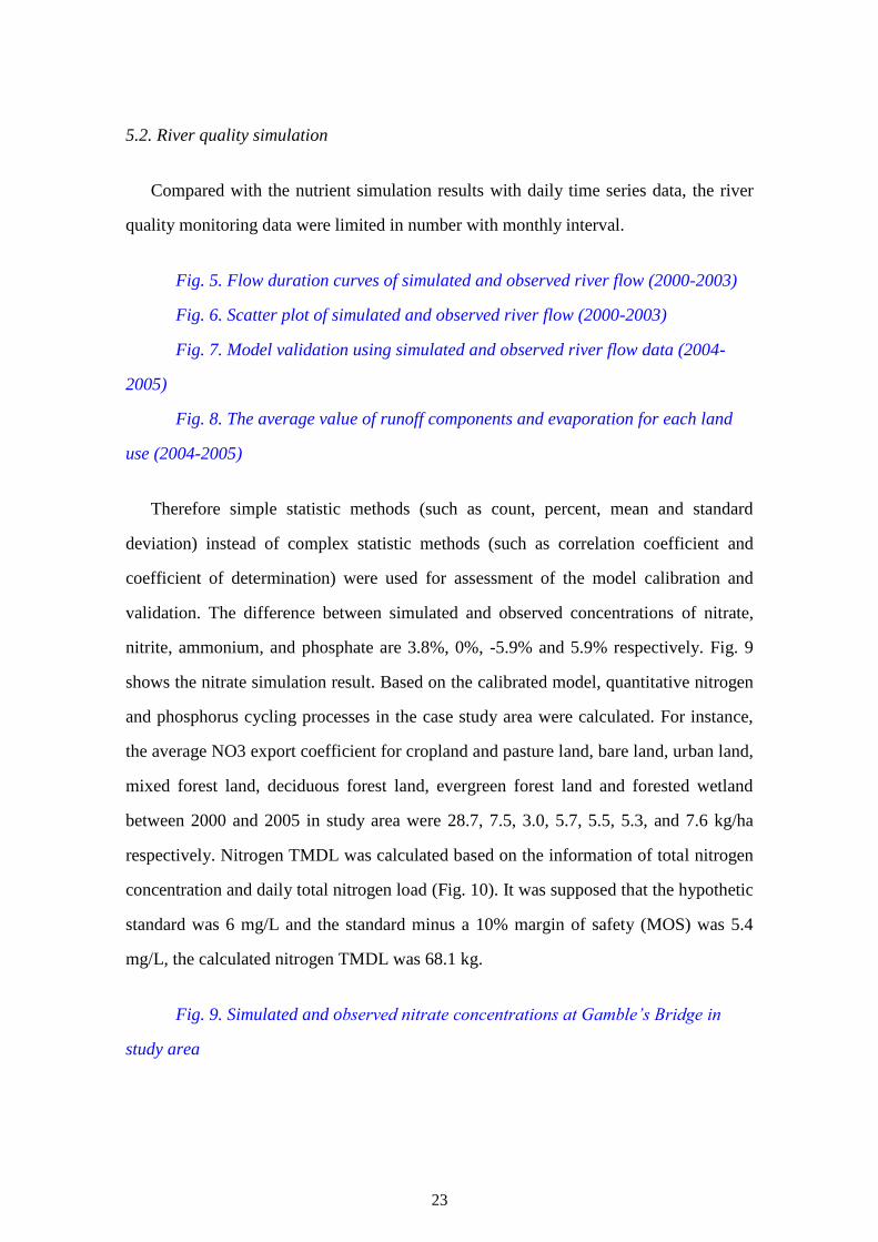
5.2. River quality simulation

Compared with the nutrient simulation results with daily time series data, the river

quality monitoring data were limited in number with monthly interval.

Fig. 5. Flow duration curves of simulated and observed river flow (2000-2003)

Fig. 6. Scatter plot of simulated and observed river flow (2000-2003)

Fig. 7. Model validation using simulated and observed river flow data (2004-

2005)

Fig. 8. The average value of runoff components and evaporation for each land

use (2004-2005)

Therefore simple statistic methods (such as count, percent, mean and standard

deviation) instead of complex statistic methods (such as correlation coefficient and

coefficient of determination) were used for assessment of the model calibration and

validation. The difference between simulated and observed concentrations of nitrate,

nitrite, ammonium, and phosphate are 3.8%, 0%, -5.9% and 5.9% respectively. Fig. 9

shows the nitrate simulation result. Based on the calibrated model, quantitative nitrogen

and phosphorus cycling processes in the case study area were calculated. For instance,

the average NO3 export coefficient for cropland and pasture land, bare land, urban land,

mixed forest land, deciduous forest land, evergreen forest land and forested wetland

between 2000 and 2005 in study area were 28.7, 7.5, 3.0, 5.7, 5.5, 5.3, and 7.6 kg/ha

respectively. Nitrogen TMDL was calculated based on the information of total nitrogen

concentration and daily total nitrogen load (Fig. 10). It was supposed that the hypothetic

standard was 6 mg/L and the standard minus a 10% margin of safety (MOS) was 5.4

mg/L, the calculated nitrogen TMDL was 68.1 kg.

Fig. 9. Simulated and observed nitrate concentrations at Gamble’s Bridge in

study area

24

5.3. Scenario results

The evaluation result of climate change scenario shows that when the annual mean

temperature increase 3°C the yearly total runoff volume of five years will decrease by

8%, 12.9%, 10.2%, 13%, 11.2% respectively (Fig. 11), and the mean daily river flow of

five years will decrease by 11.4% from 3.5 m3/s to 3.1 m

3/s.

In the land use change scenario, the mean river concentration of nitrate, nitrite, NH4

and PO4 in five years decreased by 19.4%, 33.3%, 31.3% and 31.3% respectively (Fig.

6.12). In BMP scenario, the reduction of the mean concentration of nitrate, nitrite, NH4

and PO4 in five years were 15.3%, 33.3%, 31.3% and 5.6% respectively.

Fig. 10. A simplified nitrogen TMDL calculation

Fig. 11. The impact of climate change on yearly total runoff volumes

Fig. 12. Variation of nitrate at Gamble’s Bridge over 5 years for the land use

change scenario

6. Discussions

Being one of few watershed models capable of simulating land processes and

receiving water processes simultaneously, HSPF, a free of charge model, can be used

for water quantity and quality (from both diffuse and point pollution sources) simulation

at catchment/watershed that contains both agricultural and urban land use. The results of

HSPF evaluation in this study shows that the calibrated HSPF can derive the

quantitative nutrient cycling in each type of land use and soil to help people better

understand the DWP mechanism before making water quality management policies in a

specific catchment/watershed. HSPF can also be applied for evaluating the impacts of

management policies on catchment water processes in the combined conditions of

climate change, land use change and BMP. In addition, there is a sound data

management component in HSPF that helps users easily manipulate a huge amount of

time series data and allows automatic data exchange between data management module

and other modules in the HSPF, hence improves the efficiency of modelling. In

25

conclusion, HSPF is a suitable surface water model for supporting the DWP

management at catchment scale.

Although there is no high-density groundwater monitoring network in the study area,

the observed groundwater nitrate concentration trend, derived from four groundwater

monitoring locations in the study area, is in line with the risk assessment result, tending

to validate the model. The groundwater monitoring data show that the nitrate

concentrations increase slightly from southeast to northwest in the study area. Within

‗very high‘ risk zones, dominant land cover types are arable horticulture (66%) and

improved grassland (24%). Arable horticulture and improved grassland in ‗high‘ risk

zones are 22% and 66%, respectively. In ‗moderate‘ and ‗low‘ risk zones, the dominant

land cover type is improved grassland, while arable land, neutral grass and open dwarf

shrub heath occupy relatively small portions of these zones.

In comparison of two types DWP controlling measures, i.e. remedial and

preventative measures, the prevention of DWP at a source level – catchment-scale is

vital for both sustainable water quality management and implementation of the EU

WFD (EHS, 2001; Defra, 2002c; Koo and O‘Connell, 2006). Once water is

contaminated, it will be very costly to clean-up and can take a long time to be restored,

especially for groundwater. Moreover, it is difficult to determine at a regional scale the

contribution of diffuse agricultural sources to water pollution. River Basin Management

Plan (RBMP), utilising the river basin as the natural unit, is the backbone of the

implementation of the EU WFD. It is timely to develop and evaluate suitable models or

methods for guiding catchment-scale water resource prevention activities to

complement the Programme of Measures in RBMP. HSPF is a suitable model for better

implementation of the EU WFD in the field of the surface water DWP management in

the UK and worldwide. Further studies are necessary for evaluating HSPF in all EU

member states before year 2015.

Each model has its advantages and disadvantages in certain aspects and with specific

applications. The selection of HSPF in this study means that HSPF is comparatively

more suitable than others at current stage for handling the DWP problems at the

26

catchment scale for better implementation of the EU WFD, rather than means that HSPF

is the best one over all other diffuse water pollution models in any aspect. HSPF has its

limitations or shortages. For example, HSPF instream model assumes the receiving

water body model is well-mixed with width and depth; application of this methodology

generally requires a team effort because of its comprehensive but complex nature; for

overland flow, model assumes one-directional kinematic-wave flow, etc. With rapid

development of diffuse water pollution models, other models (such as SWAT and

SHETRAN) might be proven as more suitable for better implementation of the EU

WFD in the future after further comparison and evaluation studies in the EU.

Since HSPF and BASINS were particularly designed for water resource studies in

the USA, some manual work (such as projection, data collection, and data format

converting) is needed to apply them in other countries. In this study, GIS hydrological

model was employed to prepare data required in BASINS. Although HSPF and

BASINS can be currently used for the implementation of the EU WFD, it may be

necessary to develop a new interface and make improvement of the HSPF model based

on its free open source code to facilitate its application in European countries in the long

run.

7. Conclusion

Based on the review of popular hydrologic models, HSPF was selected for

catchment-scale DWP modelling with agricultural diffuse sources. The assessment of

HSPF in the Upper Bann Catchment showed that HSPF can well guide the catchment-

scale management of water pollution from agricultural diffuse sources, by quantifying

nutrient biochemical cycling in different types of soil, and evaluating the impacts of

water management plans on surface water under the climate change. HSPF is suitable to

be introduced into the Programme of Measures in the RBMPs for better implementation

of the EU WFD in the UK. However, further studies are needed to assess the suitability

of applying HSFP in all EU member states. In addition, it is necessary to develop a new

27

software interface for HSPF based on its open source code, for its easy applications in

the EU member states for the long run.

Acknowledgements

The authors wish to acknowledge the assistance of the EHS, River Agency, CEH

UK, BADC for providing data used in this study. The Chang-Jiang Scholars Program

(MoE, China) and the Ministry of Science & Technology 863 Project (2007AA06Z343)

are also acknowledged for supporting this work.

References

Al-Abed N.A., Whiteley H.R., 2002. Calibration of the hydrological simulation program Fortran

(HSPF) model using automatic calibration and geographical information systems. Hydrol

Process 16, 3169–3188.

Albek, M., Öğütveren, Ü. B., Albek, E., 2004. Hydrological modeling of Seydi Suyu watershed

(Turkey) with HSPF. Journal of Hydrology 285, 260–271.

Arnold, J.G., Srinivasan, R., Muttiah, R.S., Williams, J.R., 1998. Large area hydrological modelling

and assessment Part I: model development. Journal of the American Water Resources

Association, 34 (1), 73–89.

Arnold, J.G., Williams, J.R. Nicks, A.D., Sammons, N.B., 1989. SWRRB, A Basin Scale

Simulation Model for Soil and Water Resources Management. Texas A&M Press. 255.

Barnwell, T.O., Johanson, R., 1981. HSPF: A Comprehensive Package for Simulation of Watershed

Hydrology and Water Quality. In: Nonpoint Pollution Control: Tools and Techniques for the

Future. Interstate Commission on the Potomac River Basin, 1055 First Street, Rockville, MD

20850.

Beasley, D.B., Huggins, L.F., 1981. ANSWERS Users Manual. EPA-905/9-82-001, U.S. EPA,

Region V. Chicago, IL.

Benaman, J., Shoemaker, C.A., Haith, D.A., 2005. Calibration and validation of soil and water

assessment tool on an agricultural watershed in upstate New York. Journal of Hydrologic

Engineering, 363-374.

Bicknell, B.R., Imhoff, J.C., Kittle, J.L., Jobes, T.H., Donigian, A.S., 2005. Hydrological

Simulation Program - FORTRAN version 12.2 user‘s manual, Environmental Research

28

Laboratory Office of Research and Development US Environmental Protection Agency, Athens,

Georgia 30605.

Birgand, F., 2004. Evaluation of QUAL2E. In: Parsons, J. E., Thomas, D. L., Huffman, R. L., editors.

Agricultural non-point source water quality models: their use and application. North Carolina

State University, Southern Cooperative Series Bulletin 398, pp. 99– 107.

Borowski I, M. Hare, 2007. Exploring the gap between water managers and researchers: difficulties

of model-based tools to support practical water management. Water Resour Manage 21:1049-

1074. Doi: 10.1007/s11269-006-9098-z

Brown, L.C., Barnwell Jr., T.O., 1987. The Enhanced Stream Water Quality Model s QUAL2E and

QUAL2E-UNCAS: Documentation and User Manual. Tufts University and US EPA, Athens,

Georgia.

Brun, S.E., Band, L.E., 2000. Simulating runoff behaviour in an urbanizing watershed. Computers,

Environment and Urban Systems 24, 5-22.

Campbell, N., D‘Arcy, B., Forst, A., Novotny, V., Sansom, A., 2004. Diffuse pollution- An

introduction to the problems and solutions. London: IWA Publishing.

Carsel, R.F., Smith, C.N., Mulkey, L.A., Dean, J.D., Jowise, P., 1984. User's Manual for the

Pesticide Root Zone Model (PRZM): Release 1. EPA-600/3- 84-109. U.S. Environmental

Protection Agency. Environmental Research Laboratory, Athens, GA.

Cho, J., V.A. Barone, S. Mostaghimi, 2009. Simulation of land use impacts on groundwater levels

and streamflow in a Virginia watershed. Agri Wat Manag 96, 1-11.

Choi, W, B.M. Deal, 2008. Assessing hydrological impact of potential land use change through

hydrological and land use change modeling for the Kishwaukee River basin (USA). J Environ

Manag 88, 1119-1130.

Crawford, N. H., Linsley, R. K. 1966. Digital Simulation in Hydrology: Stanford Watershed Model

IV. Technical Report 39, Department of Civil Engineering, Stanford University, Palo Alto, CA.

Dean, J.D., Huyakorn, P.S., Donigian, A.S., Voos, K.A., Schanz, R.W., Meeks, Y.J., Carsel, R.F.,

1989. Risk of Unsaturated/Saturated Transport and Transformation of Chemical Concentrations

(RUSTIC). EPA/600/3-89/048a. U.S. Environmental Protection Agency. Environmental

Research Laboratory, Athens, GA.

Defra (Department for Environment Food and Rural Affairs, UK), 2002. The Government's Strategic

Review of diffuse water pollution from agriculture in England: Agriculture and water - A diffuse

pollution review.

29

De-Kok J., S. Kofalk, J. Berlekamp, B. Hahn and H. Wind, 2009. From design to application of a

decision-support system for integrated river-basin management. Water Resour Manage

23:1781–1811. Doi: 10.1007/s11269-008-9352-7

Diogo, P.A., M. Fonseca, P.S. Coelho, N.S. Mateus, M.C. Almeida, A.C. Rodrigues, 2008.

Reservoir phosphorous sources evaluation and water quality modeling in a transboundary

watershed. Desalination 226, 200–214.

DoE and DARD UK (Department of Environment and Department of Agriculture and Rural

Development UK), 2003. A Consultation Paper on Nitrates and the Protection of Groundwaters

in Northern Ireland.

Donigian, A.S, Jr., Beyerlein, D.C., Davis, H.H., Jr., Crawford, N.H., 1977. Agricultural Runoff

Management (ARM) model version II: refinement and testing, Environmental Research

Laboratory, Athens, GA, EPA 600/3-77-098, 294p.

Donigian, A.S., Jr., Crawford, N.H., 1976. Modeling nonpoint pollution from the land surface,

Environmental Research Laboratory, Athens, GA, EPA 600/3-76-083, 280p.

Donigian, A.S. Jr., Huber, W. C., 1991. Modeling of nonpoint source water quality in urban and

non-urban areas (EPA/600/3-91/039). Athens, GA: US EPA, Environmental Research

Laboratory.

Donigian, A.S. Jr., Imhoff, J.C., 2002. From the Stanford Model to BASINS: 40 Years of

Watershed Modeling. ASCE Task Committee on Evolution of Hydrologic Methods Through

Computers. ASCE 150thNovember 3-7, 2002. Washington, DC. Anniversary Celebration.

EC (European Communities), 2000. Directive 2000/60/EC of the European Parliament and of the

Council Establishing a Framework for Community Action in the Field of Water Policy (OJ L

327, 22.12.2000).

EHS, 2001. Policy and practice for the protection of groundwater in Northern Ireland.

Even, S., G. Billen, N. Bacq, S. Théry, D. Ruelland, J. Garnier, P. Cugier, M. Poulin, S. Blanc, F.

Lamy, C. Paffoni, 2007. New tools for modelling water quality of hydrosystems: an application

in the Seine River basin in the frame of the Water Framework Directive. Science of the Total

Environment 375, 274–291.

Ewen, J., 1995. Contaminant transport component of the catchment modelling system SHETRAN.

In: Trudgill, S.T., editor. Solute Modelling in Catchment Systems, Wiley, Chichester, pp. 417–

441.

30

Ferrier, B., D‘Arcy, B., MacDonald, J., Aitken, M., 2004. Diffuse Pollution – What is the nature of

the problem? The Water Framework Directive: Integrating Approaches to Diffuse Pollution,

SOAS, London.

Gaddis, EJB, H Vladich, A Voinov, 2007. Participatory modeling and the dilemma of diffuse

nitrogen management in a residential watershed. Environmental Modelling and Software 22,

619-629.

Galbiati, L., F. Bouraoui, F.J. Elorza, G. Bidoglio, 2006. Modeling diffuse pollution loading into a

Mediterranean lagoon: Development and application of an integrated surface–subsurface model

tool. Ecological Modelling 193, 4–18.

Gallagher, M, J. Doherty, 2007. Parameter estimation and uncertainty analysis for a watershed

model. Environ Mod & Softw 22, 1000-1020.

Giupponi, C., 2005. Decision Support Systems for implementing the European Water Framework

Directive: The MULINO approach. Environmental Modelling and Software 22, 248 – 258.

HEC (Hydrologic Engineering Center), 1977. Storage, Treatment, Overflow, Runoff Model,

STORM, User's Manual, Generalized Computer Program 723-S8-L7520, Corps of Engineers,

Davis, CA.

Heinz I, M Pulido-Velazquez, J R. Lund, J Andreu, 2007. Hydro-economic Modeling in River Basin

Management: Implications and Applications for the European Water Framework Directive.

Water Resour Manage 21: 1103-1125. Doi: 10.1007/s11269-006-9101-8

Hessea, C, V. Krysanova, J. Pazolt, F.F. Hattermann, 2008. Eco-hydrological modelling in a highly

regulated lowland catchment to find measures for improving water quality. Ecological

Modelling 218, 135-148.

Im, S., Brannan, K., Mostaghimi, S., Cho, J., 2003. A comparison of SWAT and HSPF models for

simulating hydrologic and water quality responses from an urbanizing watershed. ASAE Paper

no. 032175. ASAE Annual International Meeting.

Jensen, M.E., Haise, H.R., 1963, Estimating evapotranspiration from solar radiation: Proceedings of

the American Society of Civil Engineers, Journal of Irrigation and Drainage, 89 (IR4), 15-41.

Kauppi, L., 1982. Testing the Application of CREAMS to Finnish Conditions. In: Svetlosanov, V.,

Knisel, W.G., editors. European and United States Case Studies in Application of the CREAMS

Model. International Institute for Applied Systems Analysis. Laxenberg, Austria. pp. 43-47.

Kleijnen, J.P.C., 2005. An overview of the design and analysis of simulation experiments for

sensitivity analysis. European Journal of Operational Research 164 (2), 287-300.

31

Knisel, W.G., 1980. ACREAMS, A Field Scale Model for Chemicals, Runoff, and Erosion from

Agricultural Management Systems. USDA Conservation Research Report No. 26, pp 643.

Knisel, W.G., Foster, G.R., Leonard, R.A., 1983. ACREAMS: A system for evaluating management

practices. In: Schaller, F.W., Bailey, G.W., editors. Agricultural management and water quality.

Iowa State University Press, Ames, Iowa, pp. 178- 199.

Knisel, W.G., Leonard, R.A., Davis, F.M., 1989. A agricultural management alternatives: GLEAMS

model simulations. Proceedings of the Computer Simulation Conference. Austin, Texas, pp.

701-706.

Koo, B.K., O‘Connell, P.E., 2006. An integrated modelling and multicriteria analysis approach to

managing nitrate diffuse pollution: 1. Framework and methodology. Science of the Total

Environment, 359, 1– 16.

Krause S, AL Heathwaite, F Miller, P Hulme, A Crowe, 2007. Groundwater-dependent wetlands in

the UK and Ireland: controls, functioning and assessing the likelihood of damage from human

activities. Water Resour Manage 21: 2015-2025. Doi: 10.1007/s11269-007-9192-x

Krause, S., J Jacobs, A Voss, A Bronstert, E Zehe, 2008. Assessing the impact of changes in landuse

and management practices on the diffuse pollution and retention of nitrate in a riparian

floodplain. Sci. Total Env 389, 149-164.

Lahlou, M., L. Shoemaker, S. Choudhury, R. Elmer, A. Hu, H. Manguerra and A. Parker. 1998.

Better Assessment Science Integrating Point and Nonpoint Sources—BASINS Version 1.0.

EPA-823-B-98-006. (Computer program manual). U.S. Environmental Protection Agency,

Office of Water, Washington, DC.

Leonard, R.A., Knisel, W.G., 1984. Model Selection for Nonpoint Source Pollution and Resource

Conservation. In: Proc. of the International Conference on Agriculture and Environment 1984.

Venice, Italy. pp. E1-E18.

Leonard, R.A., Knisel, W.G., Still, D.A., 1987. AGLEAMS: Groundwater Loading Effects of

Agricultural Management Systems. Trans. of the ASAE, 30(5), 1403-1418.

Luo, B., Li, J.B., Huang, G.H., Li, H.L., 2006. A simulation-based interval two-stage stochastic

model for agricultural nonpoint source pollution control through land retirement. Science of the

Total Environment 361, 38– 56.

Metcalf and Eddy, Inc., University of Florida, Water Resources Engineers, Inc., 1971. Storm Water

Management Model, Volume ICFinal Report. EPA Report 11024DOC07/71 (NTIS PB-203289),

U.S. Environmental Protection Agency, Washington, DC.

32

Mostert, E., 2003. The European Water Framework Directive and water management research.

Physics and Chemistry of the Earth 28, 523 – 527.

Nasr, A., Bruen, M., Jordan, P., Moles, R., Kiely, G., Byrne, P., 2007. A comparison of SWAT,

HSPF and SHETRAN/GOPC for modelling phosphorus export from three catchments in Ireland.

Water Research, 41 (5), 1065-1073.

Ng, H. Y. F., Marsalek, J., 1989. Simulation of the effects of urbanization on basin stream flow.

Water Resources Bulletin, 25, 117-124.

Onishi, Y., Wise, S.E., 1979. Mathematical model, SERATRA, for sediment-contaminant transport

in rivers and its application to pesticide transport in four mile and wolf creeks in Iowa. Battelle,

Pacific Northwest Laboratories, Richland, WA.

Orr P, J Colvin, D King, 2007. Involving stakeholders in integrated river basin planning in England

and Wales. Water Resour Manage 21: 331-349. Doi: 10.1007/s11269-006-9056-9

Oyarzun, R., Arumí, J., Salgado, L., Mariño, M., 2007. Sensitivity analysis and field testing of the

RISK-N model in the Central Valley of Chile. Agricultural Water Management 87, 251-260.

Patterson, M.R., Sworski, T.J., Sjoreen, A.L., Browman, M.G., Coutant, C.C., Hetrick, D.M.,

Murphy, B.D., Raridon, R.J., 1983. A User's Manual for UTM-TOX, A Unified Transport

Model. Draft. Prepared by Oak Ridge National Laboratory, Oak Ridge, TN, for U.S. EPA Office

of Toxic Substances, Washington, DC.

Penman, H.L., 1948, Natural evaporation from open water, bare soil, and grass: Proceedings of the

Royal Society of London, Ser. A, 193(1032), 120-145.

Peterson, J.R., Hamlett, J.M., 1998. ―Hydrologic calibration of the SWAT model in a watershed

containing fragipan soils.‖ Journal of the American Water Resources Association, 34(3), 531–

544.

Rahman, M., Salbe, I., 1995. Modelling impacts of diffuse and point source nutrients on the water

quality of South Creek catchment. Environment International, Volume 21(5), 597-603.

Ribarova, I, P. Ninovb, D. Cooper, 2008. Modeling nutrient pollution during a first flood event using

HSPF software: Iskar River case study, Bulgaria. Ecol Mod 211, 241-246.

Roesner, L.A., Aldrich, J.A., Dickinson, R.E., 1988. Storm Water Management Model User's

Manual Version 4: Addendum I, EXTRAN. EPA/600/3-88/001b (NTIS PB88-236658/AS), U.S.

Environmental Protection Agency, Athens, GA.

Ross, M.A., Tara, P.D., Geurink, J.S., Stewart, M.T., 1997. FIPR Hydrologic Model: Users Manual

and Technical Documentation. Prepared for Florida Institute of Phosphate Research, Bartow, FL,

33

and Southwest Florida Water Management District, Brooksville, FL by University of South

Florida, Tampa, FL.

Shoemaker, L., Dai, T., Koenig, J., 2005. TMDL model evaluation and research needs. EPA/600/R-

05/149, National Risk Management Research Laboratory, Office of Research and Development,

U.S. Environmental Protection Agency, Cincinnati, Ohio.

Silgram, M., S.G. Anthony, L. Fawcett, J. Stromqvist, 2008. Evaluating catchment-scale models for

diffuse pollution policy support: some results from the EUROHARP project. Environmental

Science and Policy 11, 153–162.

Sohier C., Degré A., Dautrebande S., 2009. From root zone modelling to regional forecasting of

nitrate concentration in recharge flows – the case of the Walloon Region (Belgium). Journal of

Hydrology, accepted Manuscript.

Streeter, W. H., Phelps, E. B., 1925. A study of the pollution and natural purification of the Ohio

River. Public Health Bull. 146, U.S. Public Health Service, Washington D.C.

Torrecilla N. J., Galve J. P., Zaera L.G., Retamar J. F., Álvarez A.N.A., 2005. . Nutrient sources and

dynamics in a Mediterranean fluvial regime (Ebro river, NE Spain) and their implications for

water management. Journal of Hydrology, 304, 166–182.

Tzoraki, O, N.P. Nikolaidis, 2007. A generalized framework for modeling the hydrologic and

biogeochemical response of a Mediterranean temporary river basin. J. Hydrology 346, 112-121.

UK EA (UK Environment Agency), 2005. The Relationship between the land use planning system

and the Water Framework Directive. UK.

Van-Ast JA, KL Blansch, F Boons, S Slingerland, 2005. Product policy as an instrument for water

quality management. Water Resour Manage 19: 187-198. Doi: 10.1007/s11269-005-2703-8

Wang, J.L. and Yang, Y.S., 2008. An approach to catchment-scale groundwater nitrate risk

assessment from diffuse agricultural sources: a case study in the Upper Bann, Northern Ireland.

Hydrol. Process. 22, 4274–4286.

Williams, J.R., Nicks, A.D., Arnold, J.G., 1985. Simulator for Water Resources in Rural Basins.

ASCE J. Hydraulic Engineering. 111(6), 970-986.

Yanshin, A.L., 1991. The problem of hotbed effect. Proceedings of the Black Sea Symposium

Ecological Problems and Economic Prospects, The Black Sea Foundation, İstanbul, Türkiye,

299–308.

Young, R.A., Onstad, C.A., Bosch, D.D., Anderson, W.P., 1986. Agricultural Nonpoint Source

Pollution Model: A Watershed Analysis Tool. Agriculture Research Service, U.S. Department

of Agriculture, Morris, MN.

34

Yuan, D., B. Lin, R.A. Falconer, J. Tao, 2007. Development of an integrated model for assessing the

impact of diffuse and point source pollution on coastal waters. Environmental Modelling and

Software 22, 871-879.

35

Table 1

Parameter Meaning Value Unit

INFILT Infiltration parameter 8.15 – 19.05 mm/h

UZSN Upper zone nominal storage 28.8 mm

IRC Interflow recession parameter 0.65 l/day

LZSN Lower zone nominal storage 72 mm

AGWRC Groundwater recession rate 0.992 1/day

DEEPFR

Fraction of groundwater inflow to

deep recharge

0.25 -

BASETP

Fraction of remaining ET from

baseflow

0.12 -

AGWETP

Fraction of remaining ET from active

groundwater

0.1 -

KBOD20 BOD decay rate 0.1 1/h

KNO320 Denitrification rate of nitrate 0.05 1/h

KNO220 Oxidation rate of nitrites 0.05 1/h

TCNIT

Temperature coefficient for the

nitrogen oxidation rate

1.01 1/h

TCDEN

Temperature coefficient for the

denitrification rate

1.02 1/h

DENOXT

Oxygen concentration threshold above

which denitrification ceases

1.6 1/h

36

Fig. 1

Snow

Water

Quality

Tracer

Pesticide

Nitrogen

Phosphorus

Sediment

Snow

Water

Quality

Solids

Hydraulics

Conservative

Sediment

Nonconservative

BOD/DO

Temperature

Phosphorus

Nitrogen

Plankton

Carbon

Flow

Any constituent

simulated in

PERLND,

IMPLND and

RCHRES

IMPLND RCHRES PERLND BMP

HSPF application modules

37

Fig. 2

Organic matter

atmospheric

nitrogen N2

atmospheric

fixation, fertiliser,

manure, waste, and

sludge

NO-3

NH+

4

NO-2

nitrification immobilization

mineralization

removed

from

cycle by

harvesting

N2

N2O

NO

NH3

denitrification

removed

from

cycle by

leaching

volatilisation

soil surface

Nitrogen Cycle

phosphate

fertiliser,

weathering of

phosphate rocks

PO-4

mineralization

removed

from

cycle by

harvesting

removed

from

cycle by

leaching

soil surface

Phosphorus Cycle

organic

matter

immobilization

residues

decomposition

and excreta

insoluble

phosphate

38

Fig. 3

Fig. 4

39

Fig. 5

Observed flow (m3/s)

Simulated flow (m3/s)

100

0.5 2 5 10 20 30 50 70 80 90 95 98 99.5

1

10

0.01

0.1

Percent chance flow (m3/s) exceeded

Flo

w (

m3/s

)

Fig. 6

Y = 0.942 X + 0.332

Corr Coef = 0.857 48

0 12 24 36 48 60

24

60

36

0

12

Sim

ula

ted

flo

w (

m3/s

)

Observed flow (m3/s)

40

Fig. 7

Observed flow (m3/s)

Simulated flow (m3/s)

12

0

24

36

60

48

J F M A M J J A S O N D

D J F M A M

2005 2004

Flo

w (

m3/s

)

Fig. 8

0%

10%

20%

30%

40%

50%

60%

70%

80%

90%

100%

cropland

and

pasture

transitional

area

mixed

urban

mixed

forest land

deciduous

forest land

evergreen

forest land

Evaporation

Baseflow

Interflow

Surface runoff

41

Fig. 9

Observed value

Simulated value

NO

3 (

mg

/l)

0

15

2000 2001 2002 2003 2004 2005

12

9

6

3

Fig. 10

Observed total nitrogen

Flo

w (

m3/s

)

0

2000 2001 2002 2003

Tota

l n

itro

gen

con

cen

trati

on

(m

g/l

)

Dail

y t

ota

l n

itro

gen

load

(k

g)

6

18

12

24

30

0

30

60

Simulated total nitrogen

Daily total nitrogen load

Standard = 6 mg/l

Standard - MOS = 5.4 mg/l

82

163

245

327

409

490

572

654

735

817

0

42

Fig. 11

0.0E+00

2.0E+07

4.0E+07

6.0E+07

8.0E+07

1.0E+08

1.2E+08

1.4E+08

1.6E+08

1.8E+08

Year 1 Year 2 Year 3 Year 4 Year 5

Original

Climate Change

Ye

arl

y to

tal ru

no

ff v

olu

me

s (

m

3)

Fig. 12

Year1 Year2 Year3 Year4 Year5

Original value

Land use change scenario value

NO

3 (

mg/l

)

0

12

9.6

7.2

4.8

2.4