The Nu Model for Probabilistic DataIntegration

Evgenia I. Polyakova and Andre G. Journel

Stanford Center for Reservoir Forecasting

May 2006

Abstract

The general problem of data integration is expressed into that of combin-ing prior probability distributions conditioned to each individual datum ordata event into a posterior probability for the unknown conditioned jointlyto all data. Any such combination of information requires taking into ac-count data redundancy within the information utilized. The nu expressionprovides an exact analytical representation of such combination. This expres-sion allows a clear and useful separation of the two components of any dataintegration algorithm: data information content and data redundancy, thelatter being different from data dependence. Any estimation workflow thatfails to address the data redundancy is not only sub-optimal, but may re-sult in severe bias. The nu expression reduces the possibly very complex jointdata redundancy to a single multiplicative correction parameter ν0 whose an-alytical expression is given; availability of such expression provides avenuesfor its determination or approximation. The case ν0 = 1 includes but is morecomprehensive than data conditional independence; it delivers a more robustapproximation in presence of actual data redundancy. An experiment wherethe exact results are known allows checking the results of the ν0 = 1 approx-imation against two traditional estimators based on data independence andconditional independence.

1

1 Introduction

Combining information from different sources is a challenging yet un-avoidable task in many scientific fields. Statisticians view this problem ascombining prior and pre-posterior probabilities into a posterior probability.Conveniently, practitioners often assume some form of data independenceto obtain the posterior probabilities, which may lead to incorrect and of-ten non-conservative conclusions if redundancy between data actually exists.In geology, there are rarely satisfying grounds to assume any type of dataindependence. Different data events that are related to common geologicalorigins are rarely independent. From one location to another nearby loca-tion geological structures are related one to each other leaving us with thechallenge of building posterior probabilities that do not start by assumingindependence.

The assumption of data independence is routinely used, for example, inlinear regression theory, being at the origin of name ”independent variables”.The independence assumption was overcome (only to a degree) by intro-ducing the variogram/covariance concept which removes linear dependencebetween any two data locations in space. However, complex geological struc-tures whose description involves multiple locations in space were beyond thereach of this traditional two point geostatistics until the recent introductionof multiple-point geostatistics.

All uncertain information can be coded into conditional probabilities.Thus, the problem of combining such probabilities becomes the crucial issue.One simplistic solution for the combination is to consider weighted linearaverages of prior probabilities to obtain the final posterior conditional prob-ability. For example, assume we are trying to find the probability P (A | B, C)conditioned to the two data events B and C. A possible solution is:

P (A | B, C) = λ1P (A | B) + λ2P (A | C)

For such linear combination to be valued between [0, 1], one typically re-stricts the weights λ to be positive and sum to one which entails convexity ofthe result: the combined probability is valued in the interval defined by thetwo prior probabilities P (A | B) and P (A | C). Such convexity is undesirablebecause it precludes the possibility of compounding, a the high probabilityP (A | B) by a concordant information carried by P (A | C), into a combined

2

probability P (A | B, C) higher than both.

The tau model initially introduced by Bordley (1982) then independentlyand further developed by Journel (2001) was a break-through point. It al-lowed a simple solution to the problem of combining prior probabilities withthe resulting posterior probability being always licit and accounting not onlyfor the individual information brought by the different data sourced but alsofor data redundancy through the tau weights.

This tau model remained a model, that is an approximation of the exactconditional probability given all data events taken jointly, until the seminalcontribution of Sunderrajan Krishnan (2005). Sunder established the closureof the tau model by giving the exact analytical expression of the tau weights.In other words, with the exact values for the tau weights, the tau model isactually not anymore a model, instead it provides an exact representationof the combined probability. From their exact expression, avenues for deter-mining or approximating the tau weights can be proposed.

The tau expression demonstrates that the tau weights are indeed linkedto data redundancy. The interpretation and full practical impact of Krish-nan’s fundamental result are not yet fully understood. In the present study,a cousin formulation, the nu expression is proposed which is a simpler versionof the tau expression. The nu weights are investigated as measures of spatialredundancy. We hope to gain a better prospective on the nu formulationsignificance which would help in the determination or approximation of thenu or tau parameters.

3

2 The nu representation

In this paper, the nu representation is proposed as a measure of spatialredundancy. The nu expression is derived directly and independently of theoriginal tau model although it is strictly equivalent to the latter. The nu ex-pression is appealing because its derivation is more straightforward than thatof the tau model. Moreover, the nu model puts forward a single correctionparameter (ν0) accounting for global data redundancy and independent ofthe data sequence. To establish the nu expression, first define the distancesto the unknown event (A) after observing any single data event Di:

x0 = 1−P (A)P (A) = P (A)

P (A) ∈ [0,∞]; prior distance to A occuring

xi = 1−P (A|Di)P (A|Di)

= P (A|Di)P (A|Di)

∈ [0,∞]; updated distance knowing datum Di

x = 1−P (A|D1,...,Dn)P (A|D1,...,Dn) = P (A|D1,...,Dn)

P (A|D1,...,Dn) ∈ [0,∞]; updated distance knowing

jointly all n data Di

where A = nonA and P (A | Di) is the short notation for P (A = a | Di = di):probability of A taking the value a given that datum Di takes the value di.As a consequence, all subsequent expressions are both a-value and di-datavalue dependent.

Note, that a distance is but the inverse of the prior odd ratio, e.g. theodd of A occurring is

P (A)

1− P (A)=

1

x0

.

Next, consider the following exact decomposition of the joint conditionalprobability:

P (A | D1, ..., Dn) =P (A, D1, ..., Dn)

P (D1, ..., Dn)

=P (A)P (D1 | A)P (D2 | A, D1)...P (Dn | A, D1, ..., Dn)

P (D1, ..., Dn)

= P (A)

n∏i=1

P (Di | A, Di−1)

P (D1, ..., Dn)(1)

where Di−1 = {D1 = d1, ..., Di−1 = di−1}, i.e. the set of all data up to the

4

i− 1th datum Di−1.

The notation Di−1 implies a specific sequence of n data, with D1 beingthe first datum considered and Dn being the last.

Then, re-write the fully updated distance x as:

x =P (A)

n∏i=1

P (Di|A,Di−1)

P (D1,...,Dn)

P (A)

n∏i=1

P (Di|A,Di−1)

P (D1,...,Dn)

= x0

n∏i=1

P (Di | A, Di−1)

P (Di | A, Di−1)(2)

Next, define the nu parameter νi as the ratio:

νi =

P (Di|A,Di−1)P (Di|A,Di−1)

P (Di|A)P (Di|A)

(3)

where A = nonA

The denominator of expression (3) measures how datum Di discriminatesA from nonA. Thus, νi indicates how the discrimination power of Di ischanged by knowledge of the previous data Di−1. This definition of redun-dancy involves the event A being evaluated as opposed to the traditionaldefinition of data dependence which is not related to any particular event Abeing estimated. The redundancy of datum Di as per equation (3) is relatedto all previously used data Di−1, as well as to the unknown A, and is datavalues-dependent.

The denominator of equation (3) can be re-written with Bayes inversion:

P (Di | A)

P (Di | A)=

P (Di, A)

P (A)

P (A)

P (Di, A)=

P (A | Di)P (Di)

P (A)

P (A)

P (A | Di)P (Di)=

xi

x0

Hence, the exact expression (1) can be rewritten as the nu model:

x

x0=

n∏i=1

νixi

x0= ν0

n∏i=1

xi

x0, where ν0 =

n∏i=1

νi ≥ 0 (4)

5

The single parameter ν0 appears as a global redundancy correction factorindependent of the specific data sequence. There are n! possible such datasequences. Each νi parameter appears as an individual datum redundancyfactor which depends on the previously considered data, and thus is datasequence-dependent.

The following general comments can be made about the nu model:

• If νi = 1 then the datum Di contributes to the updated distance x asit would if it was independent of all previous data, that is of Di−1

• If νi > 1 then the datum Di increases the distance x compared to itsimpact in the independence case

• If νi < 1 then the datum Di decreases the distance x compared to itsimpact in the independence case

• νi = 1 requires the two ratiosP (Di|A,Di−1)P (Di|A,Di−1)

and P (Di|A)P (Di|A) to be equal to

each other, see expression (3). One sufficient (but not necessary) con-dition is conditional independence with regard to both A and A, thatis: P (Di | A, Di−1) = P (Di | A) and P (Di | A, Di−1) = P (Di | A) ∀i.The case νi = 1 requires only equality of the two previous ratios, that is:

P (Di | A, Di−1)

P (Di | A)=

P (Di | A, Di−1)

P (Di | A)= constant ∈ [0,∞] (5)

That is the relative impact of the previous data Di−1 towards the like-lihood of Di is the same whether A or A is considered. This is notconditional independence.

• ν0 = 1 does not require all νi = 1

• A single correction factor similar to ν0 could not be readily derived

from the tau model. However, the nu and tau model are the same.

Indeed, starting from the tau model:

x

x0=

n∏i=1

(xi

x0)τi with τi ∈ [−∞,∞] (6)

6

The tau-nu parameter equivalence is written:

νi = (xi

x0)τi−1, or τi =

1 + log νi

log xi

x0

, τ1 = ν1 = 1. (7)

Both tau and nu expressions are actually exact representations of thefully conditioned probability (1), with both allowing a clear and useful sep-aration of the two components of any data integration algorithm:

• Data information content xi

x0. This component would be derived from

the actual field data and measures what additional information beyond

the prior distance x0 each datum Di taken alone brings to knowledge

of the event A being assessed. Note that this information content is

linked to how Di discriminates A from nonA, and that it is A-value

and Di value dependent; indeed the complete notation is:

xi

x0=

P (Di = di | A = a)

P (Di = di | A = a)

• Data redundancy(the νi or τi parameters). This component could beborrowed, thus approximated, from proxy training images, deliveringthe physics of the joint relations A, Di, Dj. These parameters measurehow the previous data Di−1 affects the information content of datumDi, see expression (3).

Recall that the notations A, Di, Dj are actually short for the values-dependent events: A=a, Di = di, Dj = dj.

In the next section the impact of varying the correlation range of thevarious variables A, Di, Dj on each individual nu weight is studied. The datageometric configuration is fixed. In a second experiment the data geometryis varied and its impact on data redundancy is studied.

7

3 Case Study

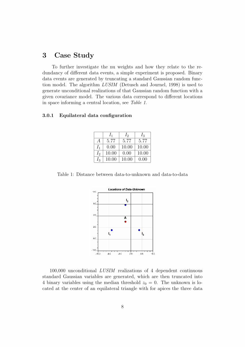
To further investigate the nu weights and how they relate to the re-dundancy of different data events, a simple experiment is proposed. Binarydata events are generated by truncating a standard Gaussian random func-tion model. The algorithm LUSIM (Detusch and Journel, 1998) is used togenerate unconditional realizations of that Gaussian random function with agiven covariance model. The various data correspond to different locationsin space informing a central location, see Table 1.

3.0.1 Equilateral data configuration

I1 I2 I3

A 5.77 5.77 5.77I1 0.00 10.00 10.00I2 10.00 0.00 10.00I3 10.00 10.00 0.00

Table 1: Distance between data-to-unknown and data-to-data

I3I1

I2

A

100,000 unconditional LUSIM realizations of 4 dependent continuousstandard Gaussian variables are generated, which are then truncated into4 binary variables using the median threshold z0 = 0. The unknown is lo-cated at the center of an equilateral triangle with for apices the three data

8

locations.

The binary indicator variables are coded as:

i (uα) =

1 if z(uα) > 00 otherwise

(8)

The indicator variable in equation (8) could, for example, state that thepresence of sand at location uα with a binary code of 1, while shale or non-sand is indicated by 0.

The semi-variogram used for simulation of the original Gaussian variable

Z(u) is an isotropic exponential model with range parameter a and unit sill:

γ(h) = 1− exp (−| h |)a

(9)

The practical range is thus 3a for which γ(3a) = 95% of the sill.

The total number of possible joint combinations of values for the fourbinary variables (A and the three indicator data I1, I2, and I3) is 24 = 16.Each of these combinations is assigned a probability of occurrence denotedpk, k = 1, ..., 16, see Table 2. The prior or marginal probability of anyone ofthese four binary variables is p0 = 0.5.

A I1 I2 I3 A I1 I2 I3

p1 0 0 0 0 p9 1 0 0 0p2 0 0 0 1 p10 1 0 0 1p3 0 0 1 0 p11 1 0 1 0p4 0 0 1 1 p12 1 0 1 1p5 0 1 0 0 p13 1 1 0 0p6 0 1 0 1 p14 1 1 0 1p7 0 1 1 0 p15 1 1 1 0p8 0 1 1 1 p16 1 1 1 1

Table 2: Joint distribution of indicators

The constraints on these probabilities are:16∑

k=1= 1 and pk ∈ [0, 1], ∀k. The

16 probabilities pk are identified to the proportions read from the 100,000realizations of the set of four indicator values (a, i1, i2, i3).

9

Concordant data values

5 10 15 20 25 300

0.2

0.3

0.4

0.5

0.6

0.7

0.8

0.9

1

Range

Pro

babi

lity

P(A | I 1I2I3)P(A | I 1)P(A | I 2)P(A | I 3)P(A)ν0=1CIFull ind

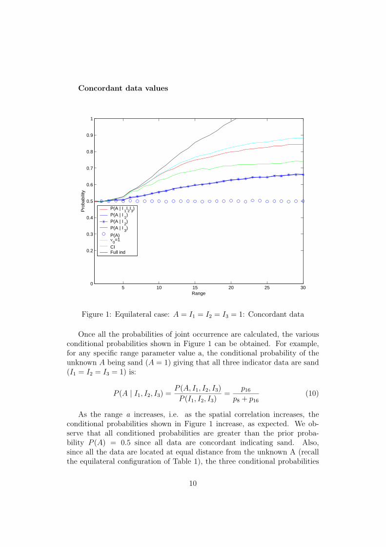
Figure 1: Equilateral case: A = I1 = I2 = I3 = 1: Concordant data

Once all the probabilities of joint occurrence are calculated, the variousconditional probabilities shown in Figure 1 can be obtained. For example,for any specific range parameter value a, the conditional probability of theunknown A being sand (A = 1) giving that all three indicator data are sand(I1 = I2 = I3 = 1) is:

P (A | I1, I2, I3) =P (A, I1, I2, I3)

P (I1, I2, I3)=

p16

p8 + p16

(10)

As the range a increases, i.e. as the spatial correlation increases, theconditional probabilities shown in Figure 1 increase, as expected. We ob-serve that all conditioned probabilities are greater than the prior proba-bility P (A) = 0.5 since all data are concordant indicating sand. Also,since all the data are located at equal distance from the unknown A (recallthe equilateral configuration of Table 1), the three conditional probabilities

10

P (A|Ij), j = 1, 2, 3 are equal for all ranges.

The fully conditioned probability P (A | I1, I2, I3) was calculated using 4different methods. First, the exact value of this probability was read directlyfrom the 100,000 realizations without any approximation. This representsthe ’true’ probability and is considered as the reference for evaluating thethree approximations which follow. This true probability is shown in red inFigure 1. It reflects a compounding of the information provided by threeconcordant data I1 = I2 = I3 = 1. Each additional concordant datum makesour decision about A being sand more certain.

• The first approximation considered for the fully conditioned prob-ability stems from a hypothesis of data independence combined with ahypothesis of conditional independence given A. For lack of a betterterm, we will call that combination of hypotheses: “full independence”.The resulting approximation is written:

P ∗(A | I1, I2, I3) =P (A, I1, I2, I3)

P (I1, I2, I3)=

P (A)P (I1 | A)P (I2 | A, I1)P (I3 | A, I1, I2)

P (I1, I2, I3)

The numerator per conditional independence given A is written:P (A)P (I1 | A)P (I2 | A)P (I3 | A).

The denominator per data independence is written: P (I1)P (I2)P (I3).

Thus,

P ∗(A | I1, I2, I3) =P (A)P (I1 | A)P (I2 | A)P (I3 | A)

P (I1)P (I2)P (I3)

=P (A)P (A|I1)P (I1)

P (A)P (A|I2)P (I2)

P (A)P (A|I3)P (I3)

P (A)

P (I1)P (I2)P (I3),per Bayes’ inversion

=P (A | I1)P (A | I2)P (A | I3)

P (A)2(11)

Or, equivalently:

P ∗(A | I1, I2, I3)

P (A)=

P (A | I1)

P (A)

P (A | I2)

P (A)

P (A | I3)

P (A)(12)

11

For example, in terms of the p′ks of Table 2, the probability P (A | I1)

is obtained as:

P (A | I1) =

16∑i=13

pk

16∑k=13

pk+8∑

k=5

pk

, and P (A) =16∑

k=9pk

The resulting probability estimate (11) is shown in black in Figure1. This approximation overestimates severely the true probability asthe variogram range parameter increases. It even becomes illicit,P ∗(A | I1, I2, I3) > 1 beyond a=20. This severe overestimation is due tothe over-compounding of three concordant data values, a consequenceof the wrong assumption of data ”full independence”.

• The second approximation calls only for conditional independenceof the data, the resulting conditional probability is calculated as:

P ∗∗(A | I1, I2, I3) =P (A, I1, I2, I3)

P (I1, I2, I3)=

P (I1, I2, I3 | A)P (A)

P (I1, I2, I3)

Per data conditional independence:

P ∗∗(I1, I2, I3 | A) = P (I1 | A)P (I2 | A)P (I3 | A)

Thus,

P ∗∗(A | I1, I2, I3) =P (I1 | A)P (I2 | A)P (I3 | A)

P (I1, I2, I3)(13)

wherein terms of the p′ks of Table 2:

P (I1 | A) =

16∑i=13

pk

16∑i=9

pk

, and P (I1, I2, I3) = p8 + p16

Note, that the approximation (13) requires evaluating the difficult-to-get joint data probability P (I1, I2, I3). This joint data probability can-cels out under the additional hypothesis of data independence as usedin expression (11).

All four probabilities required by expression (13) are read directly fromthe 100,000 simulated realizations.

Figure 1 shows the results from the conditional independence assump-tion (green curve) leading to underestimation of the true probability,increasingly so for large ranges.

12

• The third approximation for the conditional probability is calcu-lated using the tau expression (6) with all tau parameters equal to 1,or equivalently the nu expression (4) with the single global parameterν0 set to 1. First the distances to A occurring are calculated as:

x0 =1− P (A)

P (A); x1 =

1− P (A | I1)

P (A | I1);

x2 =1− P (A | I2)

P (A | I2); x3 =

1− P (A | I3)

P (A | I3);

With all tau parameters set to 1, the tau model and, similarly, theν0 = 1 model give:

x

x0

=x1

x0

x2

x0

x3

x0

. (14)

The conditional probability is immediately retrieved as:

P ∗∗∗(A | I1, I2, I3) =1

1 + x(15)

The resulting probability is shown in light blue on Figure 1.

It appears that the ν0 = 1 approximation (14) is more robust (in pres-ence of actual data redundancy) than the other two classical estima-tors stemming from conditional independence-related hypotheses. Notethat the ν0 = 1 model always produces a licit probability in [0, 1]; it isalso consistently closer to the true fully conditioned probability. Recallthat Figure 1 relates to the equilateral data configuration with concor-dant data values A = I1 = I2 = I3 = 1.

One way to ensure robustness of the conditional independence approxi-mation is to standardize it by eliminating the term P (I1, I2, I3) in expression(13), Journel (2001):

P ∗∗∗(A | I1, I2, I3) =S(A)

S(A) + S(A)(16)

where S(A) = P (A)P (I1 | A)P (I2 | A)P (I3 | A)

and S(A) = P (A)P (I1 | A)P (I2 | A)P (I3 | A)

13

Were expression (16) applied to the estimation of the complement eventA = nonA, the following probability would be obtained:

P ∗∗∗(A | I1, I2, I3) =S(A)

S(A) + S(A)

which ensures that:

P ∗∗∗(A | I1, I2, I3) + P ∗∗∗(A | I1, I2, I3) = 1 (17)

Note that neither expression (16) nor (17) corresponds to conditional in-dependence. Conditional independence versus A and jointly versus A (SeeAppendix for proof) is a sufficient but not necessary condition for expression(16).

The tau model with all τi = 1 or, equivalently, the ν0 = 1 model can beshown to identify the standardized expression (16). Indeed:

P ∗∗∗(A | I1, I2, I3) =1

1+x =1

1+x1x2x3

x20

=x2

0x2

0+x1x2x3

=P (A)2

P (A)2

(P (A)2

P (A)2+ P (A|I1)P (A|I2)P (A|I3)

P (A|I1)P (A|I2)P (A|I3)

)

=P (A)2P (A | I1)P (A | I2)P (A | I3)

P (A)2P (A | I1)P (A | I2)P (A | I3) + P (A)2P (A | I1)P (A | I2)P (A | I3)

=P (A)2P (A)3P (I1 | A)P (I2 | A)P (I3 | A)

P (A)2P (A)3P (I1 | A)P (I2 | A)P (I3 | A) + P (A)3P (A)2P (I1 | A)P (I2 | A)P (I3 | A)

then simplifying out the term P (A)2P (A)2 yields:

P ∗∗∗(A | I1, I2, I3) =S(A)

S(A) + S(A)(18)

14

Comparative results:

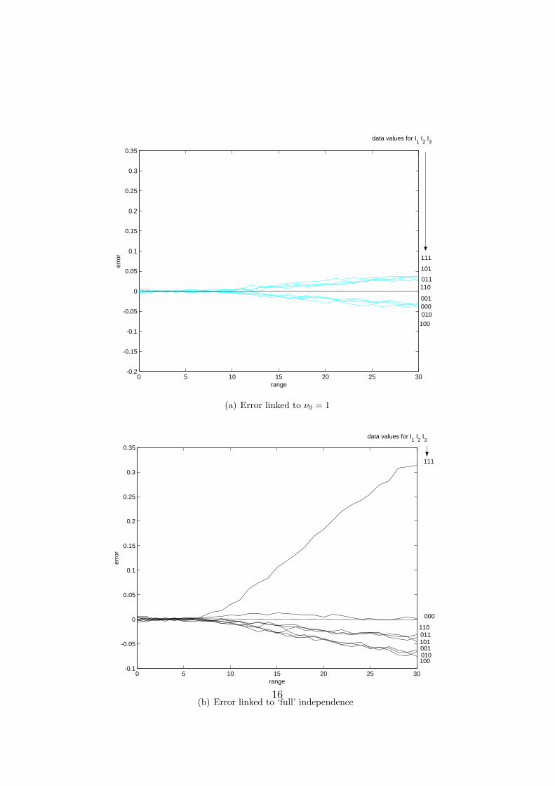
Figures 2 give the complete results corresponding to the evaluation ofthe probability of A = 1 given all 23 = 8 combinations of the 3 data I1, I2, I3.More precisely, the four Figures 2 give the deviation of the 3 approximatedprobabilities from the reference true probability:

P ∗(A | I1, I2, I3)− P (A | I1, I2, I3) vs. range parameter a

The result for A=0 can be directly deduced from the previous ones sinceP ∗(A = 0 | I1, I2, I3) = 1− P ∗(A = 1 | I1, I2, I3).

0 5 10 15 20 25 30-0.15

-0.1

-0.05

0

0.05

0.1

0.15

0.2

0.25

0.3

0.35

range

erro

r

CIFull Indν = 1

Figure 2: Approximation errors for the eight data value configurations

Figures 2 shows the ν0 = 1 approximation to be generally the best ex-cept for a few cases. The conditional independence assumption (green curve)outperforms the ν0 = 1 approximation only for the cases when any two ofthe data are equal to 0. The “full independence” assumption (black curve)performs better when all three data are equal to 0, see Figure 2b. Giventhat one is evaluating the probability of A=1, these cases correspond to

15

0 5 10 15 20 25 30-0.2

-0.15

-0.1

-0.05

0

0.05

0.1

0.15

0.2

0.25

0.3

0.35

range

erro

r

000001

010

011

100

101

110

111

data values for I1 I2 I3

(a) Error linked to ν0 = 1

0 5 10 15 20 25 30-0.1

-0.05

0

0.05

0.1

0.15

0.2

0.25

0.3

0.35

range

erro

r

000

001010

011

100

101

110

111

data values for I1 I2 I3

(b) Error linked to ‘full’ independence16

0 5 10 15 20 25 30-0.2

-0.15

-0.1

-0.05

0

0.05

0.1

0.15

0.2

0.25

0.3

0.35

range

erro

r

000

001010

011

100

101

110

111

data values for I1 I2 I3

(c) Error linked to conditional independence

non-concordant data with A=1, a state consistent with some form of dataindependence.

The two independence-based estimates deviate most from the true prob-ability when all data are equal to one. Such concordance between the 3 datavalues indicates that they should not be considered as independent whenevaluating the probability of A=1.

The ν0 = 1 estimate, although not always best, delivers robust and lowerrors for all ranges, see Figure 2a.

To investigate unbiasedness of the three approximation algorithms, weaveraged the errors of Figures 2a, b, and c over the 8 data value combina-tions, see Figure 3.

For all three approximations the average error is very small (quasi un-biasedness) for small ranges, as expected. It grows linearly beyond range

17

5 10 15 20 25 30-12

-10

-8

-6

-4

-2

0

2

4

6x 10-5

Range

erro

r

CIFull Indν0 = 1

Figure 3: Bias(error) averaged over all data values combinations. Equilateralcase.

a=10. As the range increases all values become more dependent, and thebias related to all three independence-related assumptions increases. Theν0 = 1 model, however, remains consistently the best.

18

Nu Weights:

Figure 4 shows the three data sequence-dependent nu weights calculatedusing their exact expression (3). Since there are 3 data, I1, I2, I3, informingthe unknown A, there are 3!=6 possible data sequences, hence 6 columns inFigure 4. Figure 4 relates to the case A = I1 = I2 = I3 = 1.

The first sequence given in the left most column of Figure 4 corresponds

10 20 301

1.5

2

2.51-2-3

ν 1

10 20 301

1.5

2

2.51-3-2

10 20 301

1.5

2

2.52-1-3

10 20 301

1.5

2

2.53-1-2

10 20 301

1.5

2

2.52-3-1

10 20 301

1.5

2

2.53-2-1

10 20 301

1.5

2

2.5

ν 2

10 20 301

1.5

2

2.5

10 20 301

1.5

2

2.5

10 20 301

1.5

2

2.5

10 20 301

1.5

2

2.5

10 20 301

1.5

2

2.5

10 20 301

1.5

2

2.5

ν 3

10 20 301

1.5

2

2.5

0 10 20 301

1.5

2

2.5

10 20 301

1.5

2

2.5

10 20 301

1.5

2

2.5

10 20 301

1.5

2

2.5

Figure 4: The sequence-dependent nu weights.Equilateral case: A = I1 = I2 = I3 = 1

to the ordering 1-2-3, that is I1− > I2− > I3. The first datum in anysequence always receives a unit nu weight, per definition. As the range in-creases, the redundancy between the data increases. This leads to the othertwo nu weights becoming increasingly greater than 1. Indeed, any datumIi = 1 increases the probability of A=1, hence decreases the distance toA=1. Thus, any data redundancy would limit that distance decrease, i.e.increase the distance to A=1, this is obtained with nu weights greater thanone. Also, the redundancy associated with I3 is greater than that of I2 forthe sequence 1-2-3; this results in ν3 being greater than ν2.

19

Discordant data

5 10 15 20 25 300

0.2

0.3

0.4

0.5

0.6

0.7

0.8

0.9

1

Range

Pro

babi

lity

P(A | I 1I2I3)P(A | I 1)P(A | I 2)P(A | I 3)P(A)ν0=1CIFull ind

Figure 5: Equilateral case. Discordant data: A = 1, I1 = 0, I2 = 0, I3 = 1

Recall that the exact nu weights are not only sequence-dependent butalso data values-dependent making the interpretation of these weights moredifficult. Consider now the discordant data value event corresponding toA = 1, I1 = 0, I2 = 0, I3 = 1. The corresponding conditional probabili-ties are given on Figure 5. Because two data are equal to 0, all conditionalprobabilities of having A=1, other than P (A | I3 = 1), are lesser than themarginal P (A) = 0.5. All three estimates are close to the true value, becausein presence of discordant data values the various independence hypotheses onwhich they are based become reasonable. Conditional independence appearsto give the best estimate (only slightly).

The corresponding nu weights are given on Figure 6. For all 6 possibledata sequences the nu weight associated with the discordant datum I3 =1 is approximately 1 while the other two weights are slightly less than 1decreasing with the range. Consider, for example, the sequence 1-2-3, that is

20

I1− > I2− > I3. The datum I2 = 0 increases the distance to A=1. Becauseof the redundancy of I2 = 0 with the previous datum I1 = 0, the weight ν2

is less than 1 which reduces slightly the previous increase in distance. Thedatum I3 = 1 is seen as reasonably independent of both data I1 = I2 = 0which results in the nu weight ν3 equal to 1.

10 20 301

1.5

2

2.51-2-3

ν 1

10 20 301

1.5

2

2.51-3-2

10 20 301

1.5

2

2.52-1-3

10 20 301

1.5

2

2.53-1-2

10 20 301

1.5

2

2.52-3-1

10 20 301

1.5

2

2.53-2-1

10 20 301

1.5

2

2.5

ν 2

10 20 301

1.5

2

2.5

10 20 301

1.5

2

2.5

10 20 301

1.5

2

2.5

10 20 301

1.5

2

2.5

10 20 301

1.5

2

2.5

10 20 301

1.5

2

2.5

ν 3

10 20 301

1.5

2

2.5

0 10 20 301

1.5

2

2.5

10 20 301

1.5

2

2.5

10 20 301

1.5

2

2.5

10 20 301

1.5

2

2.5

Figure 6: The sequence dependent nu weights.Equilateral case: A = 1, I1 = 0, I2 = 0, I3 = 1

21

The sequence-averaged individual weights

Figure 7 shows the individual nu weights averaged over all 6 possible datasequences for the case A = I1 = I2 = I3 = 1. These averaged nu weights areobtained by geometric averaging of the sequence-dependent weights:

νi = 6

√√√√ 6∏s=1

(νi)s (19)

where (νi)s is the nu weight for datum i in sequence s.

5 10 15 20 25 301

1.5

2

2.5

ν 1aver

age

5 10 15 20 25 301

1.5

2

2.5

ν 2aver

age

5 10 15 20 25 301

1.5

2

2.5

range

ν 3aver

age

Figure 7: Individual nu weights averaged over all data sequences.Equilateral case: A = I1 = I2 = I3 = 1

Because of the equilateral configuration, all three sequence-averaged nuweights are equal. These nu weights are increasing slightly with the rangeand are all greater than one. Indeed, because all data are equal to one theydecrease the distance to the unknown A=1, i.e. xi

x0< 1. Therefore, data

redundancy should limit that decrease, thus increase the distance to A=1:

22

this is obtained with average nu weights νi > 1.

The global nu weight ν0 for the case A = I1 = I2 = I3 = 1 is shownon Figure 8. This weight is consistent with the previous overall trends ofsequence-dependent and averaged individual nu weights: it increases withthe range. The ν0 weight is the global, sequence-independent, correctionfactor for data redundancy. Note that for small ranges, that is in presenceof spatial independence, we expect ν0 = 1. The minor fluctuations seenon Figure 8 for range a < 8 are likely due to ergodic fluctuations of ourrealizations.

0 5 10 15 20 25 30

1

1.5

2

2.5

ν 0

Range

Figure 8: The exact sequence-independent ν0 weight.Equilateral case: A = I1 = I2 = I3 = 1

23

4 Non-equilateral data configuration

I1 I2 I3

A 10.63 11.18 11.66I1 0.00 21.40 3.61I2 21.40 0.00 22.83I3 3.61 22.83 0.00

Table 3: Distances between data-to-unknown and data-to-data

I2

I1

I3

A

Figure 9: Non-equilateral data configuration

For this second example, a non-equilateral configuration of three datawas chosen to observe the impact of data locations on redundancy. Figure 9shows the data configuration, and Table 3 gives the corresponding Euclideandistances:

The study built around this data configuration is similar to that done forthe equilateral case. Figure 10 shows the conditional probabilities associatedto the case A = I1 = I2 = I3 = 1. Recall that data values concordancerepresents an unfavorable case for all independence-related approximations.

The estimate (11) based on “full independence” leads to an over-compoundingof the information Ii = 1. Conditional independence (13) gives an estimatewhich is less than the prior probability (0.5) at small ranges; this represents

24

5 10 15 20 25 300

0.2

0.3

0.4

0.5

0.6

0.7

0.8

0.9

1

Range

Pro

babi

lity

P(A | I 1I2I3)P(A | I 1)P(A | I 2)P(A | I 3)P(A)ν0=1CIFull ind

Figure 10: Non Equilateral case: A = I1 = I2 = I3 = 1

a severe error since all three individual probabilities P (A | Di) are above theprior. Again the ν0 = 1 approximation (15) provides consistently the bestestimate.

Figure 11 shows the sum P (A | I1, I2, I3)∗ +P (A | I1, I2, I3)

∗ for the threesets of estimates. That sum should be equal to 1. It appears that only the es-timate associated with ν0 = 1 verifies that consistency relation for all ranges.The two independence-based estimates (11) and (13) are not self consistent(over A and A), particularly that based on conditional independence. Thisrepresents a valuable in-built robustness of the ν0 = 1 approximation in pres-ence of data dependence.

The approximation errors for the 8 data values combinations when es-timating A=1 are plotted on Figures 12; compare to the similar Figures 2corresponding to the equilateral data configuration. Again, the conditionalprobability calculated under the ν0 = 1 assumption has more stable andsmaller errors, and conditional independence leads to the largest errors. Fig-

25

0 5 10 15 20 25 30

0.8

1

1.2

Full independence

ν0=1

Conditionalindependence

Figure 11: Checking the consistency relation.Case A = I1 = I2 = I3 = 1

ure 12a, b, and c give the errors specific to each estimate with indication ofthe 3 data values.

The errors associated with the ν0 = 1 estimate (15) are small and centeredaround 0, see Figure 12 a. That error is smallest when the two close-by dataare different (I1 6= I3), corresponding to data values not conflicting with theunderlying data independence-related hypothesis. The ν0 = 1 model appearsto downplay the contribution of the isolated I2 datum value: on Figure 12athe two error curves for I2 = 0 and I2 = 1 are similar for any given combina-tion of the I1, I3 data values. The smallest errors for the ν0 = 1 model arerelated to cases of non-concordant data values, particularly non-concordantI1 and I3 values, e.g. 0-0-1 and 1-1-0.

Figure 12b shows the errors for the “full independence” estimate. Theerror is largest for the case of concordant data A = I1 = I2 = I3 when theassumption of data independence is most likely invalid.

The most significant result is the large error associated to the conditional

26

0 5 10 15 20 25 30-0.2

-0.1

0

0.1

0.2

0.3

0.4

0.5

erro

r

range

CIFull Indν0 = 1

Figure 12: Approximation errors for the eight data value configurations

0 5 10 15 20 25 30-0.06

-0.04

-0.02

0

0.02

0.04

0.06

range

erro

r

000

001

010

011

100

101

110

111

data values for I1, I2, I3

(a) Error linked to ν0 = 1

27

0 5 10 15 20 25 30-0.1

-0.05

0

0.05

0.1

0.15

range

erro

r

000

001

010

011

100

101

110

111

data values for I1, I2, I3

(b) Error linked to ‘full’ independence

0 5 10 15 20 25 30-0.2

-0.1

0

0.1

0.2

0.3

0.4

0.5

range

erro

r

000

001

010

011

100

101

110

111

data values for I1, I2, I3

(c) Error linked to conditional independence28

5 10 15 20 25 30-1

0

1

2

3

4

5

6

7x 10-4

Range

erro

r

CIFull Indν0 = 1

Figure 13: Bias(error) averaged over all data values combinations. Non equi-lateral case.

29

independence estimate, see Figure 12c. The errors are much larger and moreunstable than for the other two estimates. Also, the positive errors associatedwith overestimation of the true conditional probability are much higher thanthe negative errors associated with underestimation leading to an overall bias.

Figure 13 shows the bias or error averaged over the 8 data value combina-tions when estimating A=1. On average the ν0 = 1 model (15) and the “fullindependence” model (11) provide reasonably unbiased estimates, while theestimate based on conditional independence leads to a severe overestimation.

30

5 Conclusions

This study allows us to draw several conclusions which may have a sig-nificant impact on how we address the problem of data integration in thefuture. Combining the contributions of data events of different sources isby no means a simple task. Each of these data events could be quite com-plex and their contributions are generally related to one another, and, thussomewhat redundant. The traditional conditional independence and “full”independence hypotheses lead to combination algorithms that are non ro-bust. In the presence of data redundancy, these hypotheses may result intheoretical inconsistencies such as probability values that are greater than 1.

The proposed ν0 = 1 model is remarkably simple, verifies all limit proper-ties of probabilities, and consistently outperforms the models based on inde-pendence assumptions. The contribution of the nu representation comparedto the tau representation is to reduce the impact of joint data redundancy toa single correction parameter ν0 whose exact expression is known. The ap-proximation ν0 = 1 appears to deliver robust estimates even in the presenseof actual data redundancy. There remains to define algorithm for estimatingthat single value ν0 whose exact analytical expression is known. As to makean independence hypothesis the ν0 = 1 model approximation is best!

Further experience from both real and synthetic data sets will provide abetter understanding about the concept of data redundancy and how it canbe approximated from the exact nu or tau expression.

31

6 References

[1] R.F. Bordley. A multiplicative formula for aggregating probabilityassessments. Management Science, 28(10):1137-1148, 1982.

[2] C. Deutsch and A.G. Journel. GSLIB: Geostatistical software libraryand user’s guide Oxford University Press, 1998.

[3] A.G. Journel. Combining knowledge from diverse sources; an alter-native to traditional data independence hypothesis. Math. Geol., Vol. 34-5,pp. 573-596., 2002.

[4] S. Krishnan. Combining diverse and partially redundant informationin the earth sciences. Ph.D. dissertation, University of Stanford, 2005.

32

7 Appendix

Notations:

In order to establish the relations between independence and conditionalindependence, let’s first introduce some notations. Let

B∐

C means B and C are independentB

∐C | A means B and C are conditionally independent given A

1. If two data events B and C are independent (that is B∐

C) we cannotconclude that these events are conditionally independent with regardto A or A . Neither can we conclude that these two data events lead tothe unit tau/nu weights. Opposite relations also does not hold. Thatis the conditional independence of B and C with regard to A or Aor ν0 = 1 model does not lead to the independence of these two dataevents.

6= . 6= .B

∐C | A

/ 6= / 6=ν0 = 1 model

6= . 6= .B

∐C B

∐C | A

/ 6= / 6=

6= .ν0 = 1 model

/ 6=

That is, independence, conditional independence and ν0 = 1 modelare all different models, although all three call for some independencerelation between B and C.

2. However, assuming that two data events B and C are conditionallyindependent with regard to both A and A, leads to independence ofB and C and the ν0 = 1 model.

33

= .B

∐C

/ 6=

B

∐C | A

B∐

C | A= .

ν0 = 1 model/ 6=

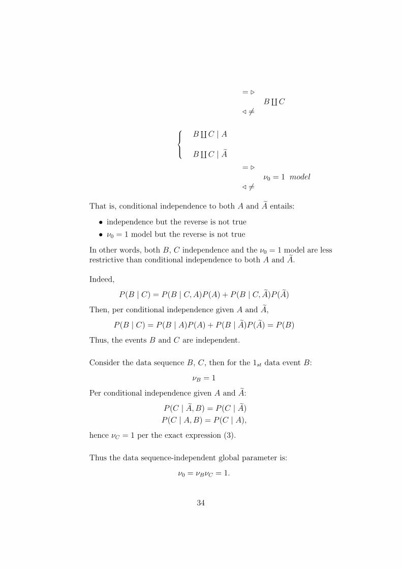
That is, conditional independence to both A and A entails:

• independence but the reverse is not true

• ν0 = 1 model but the reverse is not true

In other words, both B, C independence and the ν0 = 1 model are lessrestrictive than conditional independence to both A and A.

Indeed,

P (B | C) = P (B | C, A)P (A) + P (B | C, A)P (A)

Then, per conditional independence given A and A,

P (B | C) = P (B | A)P (A) + P (B | A)P (A) = P (B)

Thus, the events B and C are independent.

Consider the data sequence B, C, then for the 1st data event B:

νB = 1

Per conditional independence given A and A:

P (C | A, B) = P (C | A)

P (C | A, B) = P (C | A),

hence νC = 1 per the exact expression (3).

Thus the data sequence-independent global parameter is:

ν0 = νBνC = 1.

34