the novel properties of sf for directional dark matter

The novel properties of SF6 for directional dark matter

experiments

N. S. Phan1, R. Lafler, R. J. Lauer, E. R. Lee, D. Loomba, J. A. J.Matthews, E. H. Miller

Department of Physics and Astronomy, University of New Mexico, NM 87131, USA

Abstract

SF6, an inert and electronegative gas, has a long history of use in highvoltage insulation and numerous other industrial applications. Although SF6

is used as a trace component to introduce stability in tracking chambers, itshighly electronegative properties have limited its use in tracking detectors.Here, we present results with SF6 as the primary gas in a low pressure TimeProjection Chamber (TPC), using a thick GEM as the avalanche and readoutdevice. The first results of an 55Fe energy spectrum in SF6 are presented.Measurements of the drift velocity and longitudinal diffusion confirm thenegative ion drift of SF6. However, the waveform shapes have a peculiar butinteresting structure that indicates multiple drift species and a dependenceon the reduced field (E/p). The discovery of a distinct secondary peak inthe waveform, and its identification and use for fiducializing events in theTPC, are also presented. All of these properties, together with the highspin content of fluorine, make SF6 a potentially ideal gas for spin-dependentdirectional dark matter searches.

Keywords: SF6, negative ion, TPC, Thick GEMs, dark matter, WIMPs

1. Introduction

Sulfur hexafluoride (SF6) is an inert, odorless, and colorless gas com-monly known as an electron scavenger because of its large electron attach-ment cross-section. The high electron affinity coupled with its non-toxicityand non-flammability make it suitable for use in many practical applications,

1Corresponding author

Preprint submitted to October 9, 2015

some of which include a gaseous dielectric insulator in high voltage powerdevices, plasma etching of silicon and Ga-As based semiconductors, thermaland sound insulation, magnesium casting, and aluminum recycling (Refs.[1, 2] provide an extensive review of the properties and applications of SF6).In particle detectors, SF6 has been used as a quencher in Resistive PlateChambers (RPCs) operated in both avalanche and streamer modes, enablingmore stable operation by suppressing streamer formation in the former andreducing the energy of discharges and allowing lower voltage operation inthe latter [3, 4]. As a result of its many diverse commercial and researchapplications, SF6 is one of the most extensively studied gases [1].

Nevertheless, studies of SF6 in conditions applicable to particle physicsdetectors other than RPCs are scarce because the qualities that make SF6

a good insulating gas, namely its electronegativity, also make it a non-idealprimary gas in most detectors due to the difficulty of stripping the electronfrom the negative ion at the anode, a necessary first step to initiate gas gainamplification. However, with the advent of Micro-patterned Gas Detectors(MPGDs), which have flexible geometries that can sustain high electric fieldsat low pressures in the avalanche region, the potential for overcoming thisbarrier could be realized. Demonstrating sufficient gas gain in SF6 for lowenergy event detection would open up the possibility for its use in a varietyof experiments, such as directional dark matter searches.

The potential for such uses lies in some important similarities with car-bon disulfide (CS2), a negative ion gas that is currently used in the DRIFTdirectional dark matter experiment [5]. Both SF6 and CS2 are highly elec-tronegative with electron affinities of 1.06 eV for SF6, a value recommendedby Ref. [6] based on results from Ref. [7] and Ref. [8], and 0.55 eV for CS2,the latest and most precise value to date [9]. Note however that, similar toSF6, the experimentally determined electron affinities of CS2 have a largespread, ranging from ∼ 0.5 - 1.0 eV [10]. Nonetheless, both gases displaygood high voltage stability at the low pressures (< 50 Torr) necessary fordetecting directionality in the low energy nuclear recoils from dark matterinteractions.

There are, however, important differences as well. SF6 has an extremelyhigh room temperature vapor pressure of about 15,751 Torr compared toabout 300 Torr for CS2. In addition, CS2 is highly toxic and its tendency tobe absorbed into detector surfaces make operation and maintenance arduous.Moreover, for spin dependent dark matter searches, neither 12C or 32S atomshave the nuclear spin content to be suitable detection targets whereas 19F is

2

an excellent one [11]. To circumvent this, the DRIFT experiment employs amixture of 30/10 Torr CS2/CF4, whereby the advantages of the negative-ionCS2 and the spin content of fluorine can both be utilized. If the potentialof SF6 could be realized, this sacrifice of precious detection volume to thenon spin-dependent CS2 could be avoided, thereby providing a significantimprovement to the sensitivity of the experiment.

In addition to its high spin content, the electronegativity of SF6 is oneof the primary characteristics that makes it a potential alternative to CS2

for use in large-scale tracking detectors. Electronegative gases have playedan important role in directional dark matter detection as the world’s currentleading directional limit is set by the DRIFT IId detector [5], which uses amixture of CF4, CS2 and O2, with the latter two gases being electronegative.The use of CS2 in a directional dark matter detector was first suggestedby Martoff to suppress diffusion in large-scale detectors without the use ofa magnetic field [12]. In a detector with an electronegative gas, the freeelectrons produced by an ionization event are quickly captured by the gasmolecules. The negative ions then undergo thermal diffusion as they drift tothe amplification and readout region. The importance of thermal diffusion isthat it enables long drift lengths with good tracking resolution, two necessaryconditions for track reconstruction experiments and rare event searches thatrequire large detection volumes. Furthermore, electronegative gases tend todisplay superior high voltage performance over electron drift gases such asCF4 and N2 at the low pressures needed for the reconstruction of low energytracks. In fact, at pressures below about 1 atmosphere, SF6 has a breakdownfield strength that is about three times higher than air [13] and N2 [14, 15],and because diffusion in the thermal regime scales as

√L/E, where L is

the detector drift length and E is the strength of the drift field, high voltageoperation is required for the high fields needed to minimize diffusion over longdrift distances. Given the very appealing prospects of SF6, the questions thatwe wish to address in this work are:

1. Is it possible to produce avalanche multiplication in SF6 and detect anionization signal? This requires the efficient stripping of the electronfrom SF−

6 in the gain stage.

2. What is the highest achievable gas gain, and how does it depend onpressure? For example, if good gas gain can be achieved at high pres-sure, it could be of interest in other applications such as the use of SeF6

(selenium hexafluoride) for double-beta decay searches.

3

3. What is the diffusion characteristic of SF6 and how does it compare toCS2?

4. Is fiducialization of events in the drift direction attainable in SF6 and/orSF6 mixtures, and if so, under what conditions?

2. Experimental Setup and Procedure

Anode End Plate Assembly

Cathode HV End Plate Clear plastic High Voltage Shield

Field Cage Assembly

Support Saddle Assembly 1

(a) Experimental Setup

(b) Inner view of anode end plate

Figure 1

The detector used to make measurements for this work is shown in Figure1 and consists of a 60 cm long acrylic cylinder with an inner diameter of 30.5

4

cm. The ends of the detector are made from aluminum plates, one of whichserves as the cathode, which can be powered up to a maximum voltage of-60 kV. The accuracy of the reading from the front panel meter on cathodepower supply has been checked using a FLUKE 289 Multimeter with a highvoltage probe. The readings between the two meters are within about 1%at 5 kV and better than 0.1 % at 40 kV so the uncertainty in the cathodevoltage should not represent a significant systematic. The other end plate ofthe vessel is grounded and serves as the anode. The field rings are made froma kapton PC flex board that has 1.3 cm wide copper strips at 1.3 cm spacingand are connected to 23 (56 MΩ) resistors. Amplification is provided by asingle 0.4 mm thick GEM (THGEM) with a hole pitch of ∼ 0.5 mm that ismounted on two acrylic bars attached to the anode plate. The surface of theTHGEM facing the cathode is grounded to the anode plate while the othersurface is raised to high voltage. Signals are read out from the high voltagesurface with an ORTEC 142 charge sensitive preamplifier which has a 20 nsrise-time (at zero capacitance) and a 100 µs decay time constant.

Ionization can be introduced into the gas volume either from an internallymounted 55Fe 5.89 keV X-ray source (Figure 1b) or by a system using aStanford Research Systems (SRS) NL100 337.1 nm pulsed nitrogen laserilluminating the cathode. The NL100 laser has a FWHM pulse width of 3.5ns, a pulse energy of 170 mJ, and a peak power of 45 kW. The spot size inthe longitudinal, or drift, dimension is, for our purposes, essentially a deltafunction, but the projected spot size in the X and Y (lateral) dimensionsis a 1 mm x 3 mm rectangle. However, in this paper, we do not make anymeasurements involving the lateral extent of the ion cloud as it would requirewires or readout strips with multiple readout channels.

The operating procedure is as follows: After sealing up the vessel, aweekend long pump down is conducted to reduce out-gassing as much aspossible from the acrylic cylinder and other components inside the detector.The vessel is then back-filled with gas to the operating pressure, accurate to0.1 Torr, and the cathode is powered up to its operating voltage. Noting thatalthough the focus of this paper is on measurements of the basic propertiesof SF6, for comparison purposes we also present measurements made in CS2

using the same setup and operating procedure. Once the cathode is at thefull operating voltage, the detector is allowed to sit for about a half-hour toone hour to stabilize before the THGEM is powered up and measurementsare made. The measurement waveforms are acquired with a Tektronix TDS3054C digital oscilloscope and National Instruments data acquisition software

5

where every triggered event is read out and saved to file for analysis.The saved files contain the voltage signals from the ORTEC charge sen-

sitive preamplifier which integrates charge collected by the THGEM readoutsurface with a rise time of ∼ 100 ns and an exponential decay time con-stant of 100 µs. The current, I(t), entering the preamplifier is related to thedetected voltage signal, V (t), by

I(t) ∝ dV

dt−(−Vτ

), (1)

where τ = 100 µs is the decay time constant and the second term is forthe decay tail removal. We use Equation 1 to transform the acquired volt-age pulses into a current signal in software. After the conversion, pulses aresmoothed with a Gaussian filter to suppress high frequency noise. The pro-cessed waveforms are then ready for further analysis to measure drift speed,diffusion, and additional features described below.

3. Waveform Features

We measure the drift velocity by firing pulses from the SRS nitrogen laseronto the cathode. The 3.5 ns pulses generate what are essentially point-likeionization events in the longitudinal extent. The laser pulse also provides thetrigger to the DAQ system and gives us the initial time marker, T0. We definethe drift time as the time between the initial laser trigger and the arrival timeof the pulse peak, Tp, rather than the leading edge of the ionization signal atthe THGEM. The magnitude of the drift velocity, vd, is then given by

vd =L

Tp − T0

, (2)

where, L = 583 ± 1 mm, is the distance between the THGEM and thecathode. We measure the drift velocity over a range electric field values(86-1029 V/cm) for several different pressures: 20, 30, 40, 60, and 100 Torr.

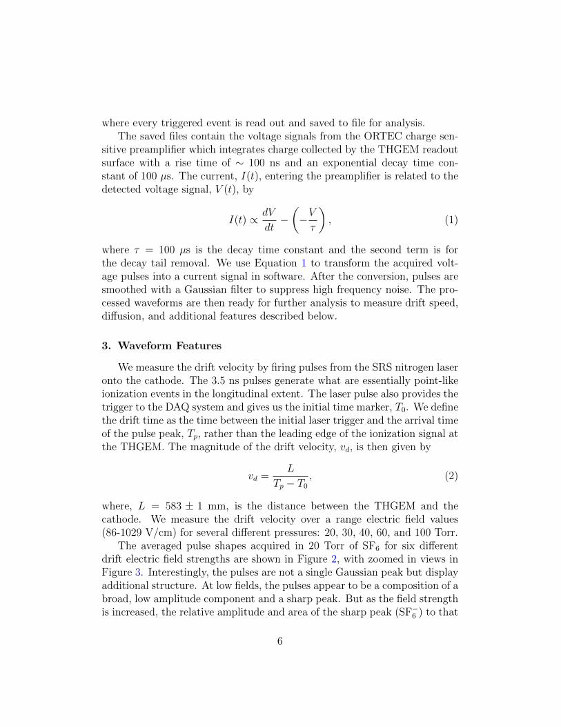
The averaged pulse shapes acquired in 20 Torr of SF6 for six differentdrift electric field strengths are shown in Figure 2, with zoomed in views inFigure 3. Interestingly, the pulses are not a single Gaussian peak but displayadditional structure. At low fields, the pulses appear to be a composition of abroad, low amplitude component and a sharp peak. But as the field strengthis increased, the relative amplitude and area of the sharp peak (SF−

6 ) to that

6

1.2 1.4 1.6 1.8

x 104

0

200

400

600

800

1000

Time (us)

I(t)

(arb

. units)

(a) E = 172 V/cm

6000 6500 7000 7500 8000

0

200

400

600

800

1000

Time (us)I(

t) (

arb

. un

its)

(b) E = 343 V/cm

4000 4500 5000 5500

0

200

400

600

800

1000

Time (us)

I(t)

(arb

. un

its)

(c) E = 515 V/cm

3000 3500 4000

0

200

400

600

800

1000

Time (us)

I(t)

(arb

. units)

(d) E = 686 V/cm

2200 2400 2600 2800 3000 3200

0

200

400

600

800

1000

Time (us)

I(t)

(arb

. units)

(e) E = 858 V/cm

2000 2200 2400 2600

0

200

400

600

800

1000

Time (us)

I(t)

(arb

. units)

(f) E = 1029 V/cm

Figure 2: 20 Torr SF6

of the broad structure also increases. However, this behavior is not onlydependent on the field strength but also on the pressure as well, and is nota simple reduced field (E/p or E/N) effect. The pulse shapes from the 30,40, 60, and 100 Torr SF6 data acquired with E = 1029 V/cm are shownin Figure 4. Besides the positive valued features, in each of Figures 2b -2f, a small amplitude dip arriving after the primary peak is observed. Thisfeature has to do with the way the THGEM is connected. The surface of theTHGEM facing the cathode and opposite the readout surface is groundedto the anode lid. Positive ions produced from the avalanche will drift awayfrom the positive voltage readout surface and towards the grounded THGEMsurface as well as the anode ground. The ions induce a small positive signal asthey move away from the readout surface but then a small negative signal isinduced as the ions approach the grounded anode end plate. This is becauseone of the THGEM surfaces is connected to the anode but is capacitivelycoupled to the readout surface.

7

Explanations for the rich structures shown in Figures 2, 3, and 4 and theirdependence on the drift field and gas pressure lie in the complex chemistryassociated with electron capture and drift in SF6 [REFs]. Although modelingof the detailed shape of the waveform is beyond the scope of this work, here wediscuss some of the chemistry that could describe some of the gross features.However, as will become clear below, a full understanding of the mechanismsleading to the observed structures eludes us at present.

Measurements made under differing conditions have shown that electroncapture by the electronegative SF6 occurs very quickly [REFs], with theimmediate product being SF−∗

6 , a metastable excited state of the anion, SF−6 ,

which is subsequently formed from the collisional or radiative stabilizationof the excited state [2]. The electron capture cross-sections by SF6 are verylarge and estimates of the capture mean-free-path are of order XXX at thepressures and drift fields of our experiments. The metastable SF−∗

6 leads tosubsequent products, besides SF−

6 , whose relative abundance depends on thelifetime of SF−∗

6 , the electron energy, gas pressure, and drift field:

SF6 + e− → SF−∗6 (attachment, metastable) (3)

SF−∗6 → SF6 + e− (auto-detachment) (4)

SF−∗6 + SF6→ SF−

6 + SF6 (collisional stabilization) (5)

SF−∗6 → SF−

5 + F (auto-dissociation) (6)

Under collision-free conditions, time-of-flight (TOF) mass spectrometricexperiments indicate the lifetime for autodetachment (4) to be between 10- 68 µs [16, 17, 18, 19, 20, 21]. Measurements made with ion cyclotron res-onance (ICR) experiments indicate the lifetime of the metastable SF−∗

6 ionto be in the ms range [22, 23, 24]. The difference in the measured lifte-time between the two techniques has to do with the experimental conditions.Specifically, the electron energies in ICR experiments are usually much lowerthan in TOF experiments [2]. For our experimental conditions, the mean-freepath, λ, which can be estimated from the measured drift speed by

λ =(3MkT )1/2 vd

eE(7)

8

[25], where T = 296 K and M is the mass of the SF6 molecule, is ∼ 0.1− 1µm, implying a collisional mean-free time of ∼ 1− 10 ns. But note that theaverage time between collisions is not necessarily the stabilization time.

1 1.5 2

x 104

0

10

20

30

40

Time (us)

I(t)

(arb

. units)

(a) E = 172 V/cm

6000 6500 7000 7500

0

10

20

30

40

Time (us)

I(t)

(arb

. units)

(b) E = 343 V/cm

4000 4500 5000

0

10

20

30

40

Time (us)

I(t)

(arb

. units)

(c) E = 515 V/cm

3000 3200 3400 3600

0

10

20

30

40

Time (us)

I(t)

(arb

. units)

(d) E = 686 V/cm

2400 2600 2800

0

10

20

30

40

Time (us)

I(t)

(arb

. units)

(e) E = 858 V/cm

2000 2100 2200 2300

0

10

20

30

40

Time (us)

I(t)

(arb

. units)

(f) E = 1029 V/cm

Figure 3: 20 Torr SF6, close up view of pre-primary peak ionization.

Reactions leading to the production of F− and SF−4 also occur but at

higher electron energies and with significantly lower probability [26, 27, 28,29], thus, we ignore them in the following discussion but return to thembelow. The cross-section for reaction (4) is peaked at zero electron energy[29, 30, 31, 33], falling by a factor of about 100 at 0.1 eV [28, 29, 32], whereasthat for reaction (6) has a peak at 0 eV [32] and a smaller one at∼ 0.38 eV [28,29, 32], with the former smaller by a factor 1000 than that for SF−

6 . Therefore,at the low electron energies expected in our experiments, SF−

6 should bethe dominant charge carrier arriving at the cathode; i.e., SF−

6 /SF−5 > 10.

Because of the higher mobility of SF−5 ([34, 35, 36], and see Section 4 below)

we should detect two peaks at the anode, with the faster SF−5 arriving earlier

9

in time. However, a number of possible reactions occurring at the start andduring drift complicate this simple picture.

3200 3400 3600 3800 4000

0

100

200

300

400

500

600

Time (us)

I(t)

(ar

b. u

nits

)

30 Torr SF6

(a) 30 Torr

4000 4500 5000 5500

0

100

200

300

400

500

Time (us)

I(t)

(ar

b. u

nits

)

40 Torr SF6

(b) 40 Torr

6000 7000 8000 9000

0

100

200

300

400

Time (us)

I(t)

(ar

b. u

nits

)

60 Torr SF6

(c) 60 Torr

1 1.5 2 2.5x 10

4

0

10

20

30

40

Time (us)

I(t)

(ar

b. u

nits

)

100 Torr SF6

(d) 100 Torr

Figure 4: Average waveforms for 30, 40 , 60, and 100 Torr at E = 1029 V/cm.

At the cathode where electrons are generated and first captured to formSF−∗

6 , auto-detachment (4) will compete with reactions (5) and (6) until allSF−∗

6 is depleted, with only stable SF−6 and SF−

5 remaining. The degree to

10

which this contributes to the pulse-shape will depend on the lifetime of SF−∗6

and the mean-free-time for collisional stabilization which are both dependenton the the pressure and drift field. If a significant fraction of the initiallyproduced SF−∗

6 auto-detaches, the free electrons will be re-captured quickly,and the process will repeat until SF−∗

6 is fully depleted via reactions (5)and (6). If the electron capture mean-free-time is indeed very short, thewaveform detected at the anode is due purely to the negative ions SF−

5 , SF−6

and SF−∗6 drifting in the chamber. If in addition we assume that the mobilities

of SF−∗6 and SF−

6 are equal, the waveform would consist of two peaks withstructure in between due to the initial phase of attachment/auto-detachment.Specifically, the main SF−

6 peak is the fraction of initially produced SF−∗6 that

eventually converts to SF−6 , and the region between it and the SF−

5 peak isfrom SF−∗

6 undergoing numerous attachments/auto-detachments, (3) and (4),before finally auto-dissociating to SF−

5 via (6) . The latter arrives between theSF−

5 and SF−6 peak because its drift velocity is a weighted average between

that of SF−∗6 and SF−

5 . A key point here is that a significant initial phase ofattachment/auto-dissociation will result in a larger fraction of SF−

5 arrivingat the anode. Thus, the SF−

5 /SF−6 ratio is, with all else equal, governed by a

competition between the probability of auto-detaching relative to collisionalstabilization, (5). The mean-free-time for the latter process should decreasewith increasing drift electric field, resulting in higher SF−

6 fraction. As weshow below, this model does explains some of our data.

A fuller picture, however, must also account for possible interactions en-gaged by the SF−

5 and SF−6 during the∼ 60 cm drift to the anode. At low drift

fields, neutral, electron-hungry SF6 molecules will form clusters around thenegative ions [REFs]. This has been observed by others, but with measuredmobilities that are lower for the resulting drifting SF−

6 (SF6)n and SF−5 (SF6)n

(n = 1, 2, 3, ...) clusters than those of SF−5 and SF−

6 [REFs]. This phenomenacould therefore explain the long tail on the slow side of the SF−

6 peak of ourlow field pulse-shapes shown in Figures 2a and 3a and the low reduced fieldpulse-shape in Figure 4d. In addition to clustering, the drifting SF−

5 andSF−

6 could also interact with the neutral gas leading to other species [REFs].Importantly, the probability of collisional detachment of energetically stableSF−

5 and SF−6 via the following reactions:

SF−5 + SF6 → SF5 + SF6 + e− (collisional detachment) (8)

SF−6 + SF6 → SF6 + SF6 + e− (collisional detachment) (9)

11

is very small for center-of-mass energies < 60 eV [37]. In comparison to theelectron affinities of SF5 (2.7− 3.7 eV) [38] and SF6 (1.06 eV), the thresholdfor detachment is much larger and is attributed to competing charge-transferand collision-induced dissociation processes [37, 39, 40]. However, there isevidence that energetically unstable states of SF−

6 (i.e. SF−∗6 ) can contribute

to collisional detachment [37, 39]. The relative contributions of these effectsdepend on the interaction energies at different reduced electric fields.

With this overview of the chemistry of electron drift in SF6, we turn to adetailed look at our data shown in Figures 2, 3, and 4. Figures 2 and 3 showthe evolution of the pulse-shapes at P = 20 Torr (N = 6.522× 1017 cm−3 atT = 296 K) as a function of drift field, and Figure 4 shows the evolution ata fixed drift field, E = 1029 V/cm, as a function of pressure. Both figuresshow a complex structure at low reduced fields that evolves to a simplerone at high reduced fields. At the highest reduced fields (Figures 2e, 2f, 3e,3f, and 4a) two peaks are clearly seen, with some charge in between and asmaller amount arriving faster than the secondary peak. The larger, lowermobility peak is SF−

6 and the smaller secondary peak is attributed to SF−5 .

To interpret how the waveform evolves with reduced field we consider Figure4 first. Naively, we would expect that increasing gas density at a fixed Ewould result in a shorter mean-free-time between collisions, allowing more ofthe SF−∗

6 to stabilize to SF−6 at the expense of auto-detachment. The shorter

mean-free-times with increasing pressure would also argue for lower electronenergies, resulting in more SF−

6 relative to SF−5 . What is observed instead is

a relative increase of charge carriers with higher mobility than SF−6 , implying

an increase in auto-detachment, SF−5 , or other species. The structure seen

in the pulse-shape in this regime, and its evolution with pressure shown inFigure 4, is not understood at this time.

The evolution of the waveform as a function of drift field at fixed P =20 Torr (Figures 2 and 3 ), however, is better fit with the model outlinedabove. There we suggested that increasing E (for fixed P ) should lead toshorter mean-free-times for collisional stabilization, (5), shifting the inter-peak charge (attributed to SF−

5 ) into the SF−6 peak. But the increase in

electron energy expected at higher E should, if significant, also result in anoverall increase in the SF−

5 fraction. Therefore, the charge lying between theSF−

5 and SF−6 peaks at low E, which was due to SF−

5 produced at the endof numerous SF−∗

6 auto-detachment reactions (4), as surmised above, willmove into the main SF−

6 peak at high E. The data in Figures 2 and 3 doshow a decrease in the inter-peak charge region and, starting at E = 515

12

400 600 800 10000.6

0.65

0.7

0.75

0.8

0.85

0.9

0.95

1

Electric Field (V/cm)

Ch

arg

e F

ractio

n

Prim. Peak Charge

Prim. + Non−Peak Charge

(a) Charge Fraction

400 600 800 10000

0.05

0.1

0.15

0.2

0.25

0.3

Electric Field (V/cm)C

harg

e F

raction

Inter−Peak Charge

Sec. Peak Charge

Pre−Sec. Peak Charge

Non−Prim. & Sec. Peak Charge

(b) Charge Fraction Low

Figure 5: The fractional charge contained in different parts of the waveform in 20 TorrSF6 as a function of the electric field. The primary and secondary peaks correspond tothe SF−

6 and SF−5 peaks, respectively.

V/cm, an SF−5 peak begins to emerge (clearer in the zoomed in Figure 3c).

By E = 1029 V/cm (Figures 2f and 3f) nearly all of the charge carriersare in the SF−

5 and SF−6 peaks, with only a small fraction lying in between.

Although Figure 3c-3f indicates that SF−5 grows with E, as expected from

our simple model, a more quantitative assessment is required.To study this we average 200 waveforms for each of seven different elec-

tric field strengths between 515-1029 V/cm, all at fixed P = 20 Torr. Theresulting averaged waveforms are divided into four regions, from left to right:the pre-SF−

5 peak region, the SF−5 peak, the area between the SF−

5 and SF−6

peaks, and the SF−6 peak. The evolution of the fraction of charge in each

region as a function of the electric field is shown in Figure 5. As predictedby our simple model, essentially all of the inter-peak charge appears to shiftover into the SF−

6 peak. However, there is no detectable change in the SF−5

peak, which suggests only a small, if any, increase in electron energies withthe drift field.

A final puzzle in our data is the charge seen on the higher mobility sideof SF−

5 . This is clearly seen in Fig. 3b-3f and, like the inter-peak charge, ittoo decreases with electric field. The fact that this charge has an edge on theleft side, i.e., a minimum drift time, implies another electronegative species

13

produced with a similar mechanism to SF−5 that competes with collisional

stabilization, (6), to SF−6 . The mobility of the charge arriving at this edge

is plotted in Figure 6 of Section 4. As mentioned above, SF−4 and F− are

also produced as in (6) for SF−5 , but with much lower probabilities. These

are both good candidates to explain this feature but unfortunately only theF− mobility has been measured (see Section 4), and it does not agree withours. Suffice it to say, a full understanding of all the processes involved inthe evolution of the waveforms seen in Figures 2-4 requires further study.For the purposes of this work, we focus on the main SF−

5 and SF−6 peaks and

their use in dark matter experiments.

4. Mobility

The mobility, µ, of a drifting ion at a specific gas density is related to thedrift speed and electric field through the relation,

vd = µ · E, (10)

where E is the electric field. By convention, rather than reporting µ or vd, thereduced mobilities, µ0, are reported instead as determined from the formula

µ0 =vdE

N

N0

, (11)

where N0 = 2.687× 1019 cm−3 is the gas density at STP (0C and 760 Torr)and N is the detector gas density at the time of measurement. Mobilitiesfor several negative ion species as a function of the reduced field (E/N) inunits of the Townsend (1Td = 10−17 V cm2, 1 V cm−1 Torr−1 = 3.066 Td atT = 296 K) are plotted in Figure 6. We find good agreement for the reducedmobility of CS−

2 in CS2 in the low field regime (< 50 Td) between our resultsand that reported by Ref. [41]. For SF−

5 and SF−6 in SF6, excellent agreement

is found with the mass-identified mobility measurements reported in Ref. [35]over the full range of our data set. A comparison of our mobilities and thosefrom Ref. [35] with mobilities reported in Ref. [34] shows agreement onlyfor reduced fields less than ∼ 60 Td for both SF−

5 and SF−6 . The same

comparison with Ref. [36] shows good agreement for SF−6 over the full range

of the data set but only up to about ∼ 60 Td for SF−5 .

In addition to the mobilities for CS−2 , SF−

5 and SF−6 , Figure 6 also contains

the mobilities for possibly another negative ion drifting in SF6, which we label

14

101

102

0.4

0.45

0.5

0.55

0.6

0.65

0.7

0.75

E/N (10−17

Vcm2)

µ0 (

cm

2 V

−1 s

−1)

χ−

SF5

−

SF6

−

CS2

−

(a) Reduced mobilities in SF6 and CS2

Figure 6: The reduced mobilities as a function of reduced field for χ−, SF−5 , and SF−

6 inSF6 and CS−

2 in CS2. The SF−5 and χ− mobilities only go down to ∼ 66 Td because the

peak and feature becomes difficult to identify at fields lower than this value. Our resultsfor SF−

5 and SF−6 are in excellent agreement with those found in Ref. [35] while the CS−

2

results agree with the result of Ref. [41].

χ−. The presence of this species is most clearly seen in Figures 3d and 3eas small steep edges arriving before the SF−

5 peak at ∼ 3150 and 2450 µs,respectively. The χ− mobility is far lower than the reported mobility for F−

in SF−6 [42] but is very close to the mobilities reported for the positive ions

SF+3 and SF+

4 [43, 44]. This is interesting because of the remarkable similarityfound between the mobilities of SF+

5 and SF−5 [35, 44], which could suggest

similar behavior for the positive and negative ions of SF3 and SF4. But at thesame time, this is unexpected because the cross-section for F− production ishigher than that for SF−

3 and SF−4 [REF]. Nevertheless, even at the highest

reduced field, there is no identifiable peak for χ−, so it is also possible that itis not actually another negative ion species in SF6 but is rather only a featureresulting from the processes responsible for the production and transport ofSF−

5 and SF−6 in the gas. Intriguingly, the mobility for this unidentified

15

species (or feature) is closely matched with the reported mobility for SF−5 in

Refs. [34] and [36] for reduced fields above ∼ 70 Td, and at the same it isworth noting that the majority or all of the data from Refs. [34] and [36] donot have mass analysis.

For a reduced field less than 60 Td, the CS−2 mobility is about 13.7%

lower than SF−6 mobility, but this difference rises to about 17.6% at about

158 Td which shows that SF−6 mobility increases more rapidly with reduced

field than CS−2 mobility. This is quite interesting because SF6, as compared

to CS2, is a much heavier molecule and the drift velocity for ions with mass,m, drifting in a gas with molecules of mass, M , follow the formula,

vd =

(1

m+

1

M

)1/2(1

3kT

)1/2eE

Nσ, (12)

where σ is ion-gas molecule cross-section [45]. This, of course, implies thatthe cross-section for SF−

6 :SF6 interaction is lower than that for CS−2 :CS2

interaction. Comparing the mobility of SF−5 to SF−

6 , we see that the mobilityof the former is 6.6% higher than the latter at about 66 Td and is 8.7%larger at about 158 Td which would indicate that SF−

5 mobility increasesmore rapidly with reduced field. At reduced fields of about 66 Td and 158Td, the χ− feature is 13.3% and 16.8% faster than SF−

6 , respectively.It is interesting to note that the behavior of the mobility with reduced

field for the negative ions in Figure 6 is in stark contrast to positive ion driftin noble gases where the drift velocity is proportional to E at low fields, whichis to say that the mobility is independent of E, but becomes proportional to√E at high fields, or that the mobility decreases as 1/

√E [45]. Of course,

the behavior of negative ion drift is complicated by the process of electroncapture as well as other processes such as ion-conversion occurring duringtransport. The capture cross-section is strongly dependent on the electronenergy, and in the case of SF−

6 , is maximal near zero-energy but decreaseswith increasing electron energy [29, 30, 31, 33]. The transport processes arealso energy dependent as can be seen with the rise in mobility with increasingreduced field for all of the negative ions in Figure 6. This has importantimplications for diffusion at high reduced fields as we show in Section 5.

5. Longitudinal Diffusion

At small field strengths where the diffusing charge cloud has thermalenergy, the diffusion coefficient at zero E/N , D(0), is related to the mobility

16

and temperature through the Nernst-Townsend-Einstein relation:

D(0)

µ(0)=kT

e, (13)

[46]. At higher field strengths, approximate relations known as the general-ized Einstein relations (GER) have the form,

DL

µ=kTLe

[1 +K

′+ ∆LK

′]

(14)

DT

µ=kTTe

[1 +

∆TK′

2 +K ′

], (15)

where K′

is the field derivative of the mobility, defined as

K′=

d lnµ0

d ln(E/N)=E/N

µ0

dµ0

d(E/N)(16)

and ∆L and ∆T are correction terms with magnitude ranging from 0 to0.20 for the longitudinal and transverse diffusion coefficients DL and DT ,respectively [47]. However, for this section we will use the expression for thediffusion coefficient in the zero field approximation given by Eq. 13. Withthat relation, a starting point-like charge cloud drifting over a distance, L,has a longitudinal diffusion width, σz, given by

σ2z = 2DLt =

4εL

3eE=

2kTL

eE, (17)

where t = L/vd and ε = 3/2kT [45]. The diffusion in the time domain, σt, isconverted to a spatial width by the simple relation,

σz = σt · vd. (18)

Customarily, diffusion is expressed by normalizing the measured value rela-tive to the drift length:

σ0 =σz√L

=

√2kT

eE, (19)

where σ0 has units of µm/√

cm.

17

At each pressure and electric field, one hundred pulses are averaged to in-crease signal-to-noise before fitting to a Gaussian curve. The diffusion width,σt, is found by subtracting, in quadrature and assuming no correlation, allother contributions from the fitted width, σfit. For us these are the electronicsshaping time, σsmooth, laser spot size, σspot, electron-capture mean-free-path,and possible effects at the THGEM. In our measurements, the laser spotsize contribution to the longitudinal width is negligible, but the latter twoeffects are not. However, we do not have the ability to determine the capturemean-free-path and the THGEM effects, so they are left out of the quadra-ture subtraction in Eq.20 but will be included as systematics with estimatesof their values given below:

σt =√σ2

fit − σ2smooth − σ2

spot. (20)

2300 2400 2500 2600 2700 2800

0

50

100

150

200

250

300

350

400

Time (us)

I(t)

(ar

b. u

nits

)

2400 2600 2800

0

10

20

30

40

50

Time (us)

I(t)

(ar

b. u

nits

)

(a) CS2 20 Torr Averaged Waveform

5700 5800 5900 6000 6100

0

100

200

300

400

500

Time (us)

I(t)

(ar

b. u

nits

)

(b) CS2 40 Torr Averaged Waveform

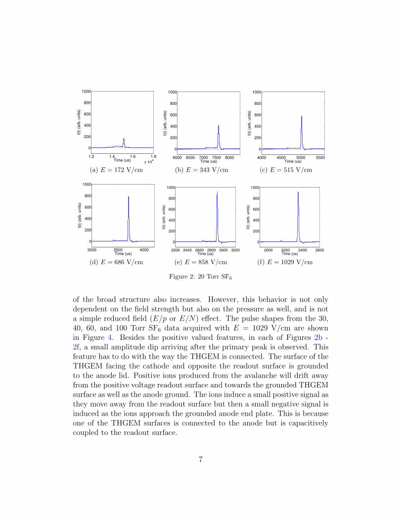
Figure 7: (a) The averaged waveform for 20 Torr CS2 at E = 1029 V/cm showing thepresence of a large secondary peak at ∼ 2600 µs and the possible appearance of twoadditional peaks at ∼ 2660 µs and ∼ 2520 µs (inset). In addition, the distortion in thewaveform shape is clearly seen in both the primary and secondary peaks at this highreduced field. (b) The average waveform for 40 Torr CS2 at E = 1029 V/cm which showsno clear secondary peaks or distortion in waveform shape.

Besides the systematic effects, the quadrature subtraction could also bea source of bias because the pulse width is not truly Gaussian, but appears

18

to exhibit a tail on the right side due to an induced signal caused by ionsdrifting away from the THGEM readout. The ion tail is a feature that is alsoobserved in [41]. To exclude the induced signal, we fit only the left hand sideof the pulse up to the peak. Besides the long ion tail, we showed in Section 3that the pulses in SF6 contain additional structure that tends to grow withdecreasing reduced field, making it difficult for fitting. Thus, we only fit thedata for E > 500 V/cm at 20 Torr and E = 1029 V/cm at 30 and 40 Torr.By performing multiple fits of the waveform with different smoothing widths,we estimate that the error introduced by subtracting the smoothing width,σsmooth, to be about XX mm.

For a comparison, we also fit the 40 Torr CS2 data (Figure 7b) but notthe 20 Torr data because of distortion in the waveform at high fields (Figure7a). The smaller, secondary peak at ∼ 2600 µs in Figure 7a is a new featurediscovered here, which could be another species of negative ion in CS2 (e.g.CS− produced similarly to SF−

5 via auto-dissociation (Eq.6) that is createdat high reduced fields. This secondary feature first appears at a drift field ofE = 343 V/cm at 20 Torr CS2 and has a drift speed that is ∼ 6.2% fasterthan, and an amplitude only 0.4% that of the primary peak value. When thedrift field is increased to E = 686 V/cm, the secondary peak’s drift speedand amplitude increase to 6.8% and 4.6%, respectively, relative to that of theprimary peak. Finally, at E = 1029 V/cm, the secondary peak is about 7.5%faster than the primary while its amplitude continues to grow and reachesabout 11.7% of the primary’s peak value (Figure 7a).

The results for E = 1029 V/cm are shown in Table 1. The second columncontains widths where no attempt was made to subtract non-diffusion relatedcontributions from σz, which are discussed below. At 40 Torr SF6(CS2), thevalue of σz = 0.74(0.73) mm corresponds to a temperature of 556(541) K.This is of course much higher than the ambient room temperature and anexpected σz of 0.54 mm for thermal diffusion, but is not surprising due tothe neglected contributions to pulse width mentioned above.

The two possible main sources of systematics contributing to the pulsewidth are the electron-capture mean-free-path and distortions in the unifor-mity of the drift field due to the dipole contributions from the holes in theTHGEM. Here we place bounds on the sum of these contributions. For CS2,the capture distance could be as large as 0.35 mm in 40 Torr [41], but wedo not know this value for SF6. By subtracting in quadrature the expectedσz and the capture length from the measured value of 0.73 mm in 40 TorrCS2, we estimate that the lower bound on the systematic could be at least

19

0 0.5 1 1.5 2 2.5 3

x 10−3

0

0.2

0.4

0.6

0.8

1

1.2

1/E (cm/V)

σz2 (

mm

2)

(a) CS2 40 Torr

Figure 8

Table 1: Diffusion widths and coefficients for 20-40 Torr SF6 and 40 Torr CS2 at E = 1029V/cm and L = 58.3 cm. The corrected σz (third column) is derived by subtracting theestimated σother = 0.43±0.12 mm, in quadrature, from the measured σz (second column).

Pressure [Torr] σz [mm] Corrected σz [mm] DL [cm2s−1]

20 SF6 1.19 1.11 2.6430 SF6 0.85 0.73 0.7640 SF6 0.74 0.60 0.3940 CS2 0.73 0.59 0.29

0.34 mm. The upper bound due to the THGEM is determined by assuminga zero capture length, and this gives a value of 0.49 mm. It is by no coin-cidence that the thickness of the THGEM (0.4 mm) lies within this rangewhile the THGEM pitch (0.5 mm) is close to the upper bound. The contri-bution from the field near the THGEM can be modeled, and the sum total ofnon-diffusion contributions can be determined by measuring the pulse-widthas a function of drift distance. This is left for future work.

20

However, we can estimate in another way all contributions to the pulsewidth aside from diffusion by plotting σ2

z as a function of inverse of theelectric field, 1/E, as shown in Figure 8a for the 40 Torr CS2 data. Sinceσ2

z is proportional to 1/E, in the limit that E → ∞, diffusion goes to zeroand the vertical-intercept in Figure 8a gives the value of the square of theother contributions, σ2

other, that are independent of electric field. We fit thedata points in Figure 8a to a linear curve and obtained a value of σother =0.43± 0.12 mm, which is very close to our previous estimate of the THGEMfield contribution to pulse width. The slope of the fit in Figure 8a gives atemperature of 330 ± 25 K for 40 Torr CS2 and nearly the same value for40 Torr SF6, both consistent with room temperature. The corrected σz’s areshown in the third column of Table 1 while the fourth column contains thecorresponding diffusion coefficients. It is worth noting that the validity ofapplying the 40 Torr data correction value to the 30 and 20 Torr data isquestionable as the systematics due to electron capture length and THGEMfield effects are likely reduced field dependent.

A similar treatment of the SF6 data would require fitting the pulses overa comparable range of E, but the non-Gaussian shape of the signals at lowE prevents this. Nevertheless, the similar values of σz for SF6 and CS2 at 40Torr (Table 1) suggest that the diffusion behavior of the two gases are quitesimilar. But it should be noted that the assumption of thermal diffusioncould break down at higher E/P. A possible indication of this is the observedrise in the reduced mobility with increasing reduced field shown in Figure6. This has important consequences for directional dark matter experimentswhere the requirement of both long drift distances and low diffusion can bemet if thermal diffusion extends to the highest drift fields possible. Thisrequires further investigations left for future work.

6. Gas Gain

Previous works have shown that gas gains greater than 1000 can beachieved in electronegative gases with proportional wires [56], GEMs [57],and bulk Micromegas (Micro Mesh Gaseous Structure) [58]. In contrast toelectron gases where only moderate electric fields of order 100 V cm−1Torr−1

are needed to accelerate electrons to energies close to the ionization potentialof the gas, electronegative gases require much higher electric fields to initiateavalanche even though the electron affinity is usually much lower than theionization potential [59]. The reason for this lies in the difficulty of initiat-

21

ing the avalanche by detaching the electron from the negative ion, which isthermally coupled to the gas. For CS2, measurements show that the pressurereduced minimum field, Emin/P , needed to initiate avalanche is over one or-der of magnitude larger than for the electron drift gas P10 (10% Methane inArgon) [59]. A similar study can be done for SF6, but in this section we omita discussion of the detailed mechanism for avalanche in this gas and insteadfocus on the gas gains that were achieved.

The gas gain in SF6 is measured with the use of an 55Fe 5.89 keV X-raysource. To convert the energy of the X-ray into the number of electronsproduced during the ionization process, we make use of the W-factor, whichis defined as the mean energy required to create a single electron-ion pair.For SF6, this value has been measured using α particles [60] and a 60Coγ source [61]. Those measurements give Wα = 35.45 eV and Wγ = 34.0eV, respectively. The slight disagreement is actually consistent with othermeasurements of W-factors which find that Wα exceeds Wγ,β for moleculargases [62]. Because we are using an X-ray source, we will adopt the W-factorfrom Ref. [61], so the average number of primary electrons, Np, created byan 55Fe X-ray interaction in SF6 is

Np =E55Fe

Wγ

=5.89 keV

34.0 eV' 173. (21)

The effective gas gain is then given by,

Geff =Ntot

Np

, (22)

where Ntot is the total number of charges read out with the preamplifier.In general, Ntot is less than the total number of charges produced in theavalanche due to an imperfect efficiency for collecting the charges, hence,the measured gain is an effective and not an absolute value. In our case,we are essentially collecting all of the electrons produced in the avalanche,but there is an additional contribution to the pulse shape from the positiveions that are also produced. To determine Ntot from a measured pulse’sV(t), the standard calibration procedure of injecting a known charge intothe preamplifier is used. In this case, we used an ORTEC 448 ResearchPulser to inject charge into the 1 pF calibration capacitor inside the ORTEC142 preamplifier.

For each pressure, we raised the GEM voltage until highly energetic sparksare observed and/or until the rate of micro-sparks and background events

22

200 400 600 8000

20

40

60

80

100

120

140

160

180

200

Charge (arb. units)

Co

un

ts

55Fe Spectrum30 Torr SF6

1 mm THGEM

∆ V = 1005 V

(a) 30 Torr SF6 1 mm THGEM

200 400 600 8000

50

100

150

200

250

300

350

400

Charge (arb. units)C

ou

nts


0.4 mm THGEM

∆V = 820 V

(b) 30 Torr SF6 0.4 mm THGEM

200 400 600 8000

50

100

150

200

250

300

350

Charge (arb. units)

Co

un

ts


0.4 mm THGEM

∆ V = 880 V

(c) 40 Torr SF6 0.4 mm THGEM

200 400 600 8000

20

40

60

80

100

120

140

160

180

200

Charge (arb. units)

Co

un

ts


0.4 mm THGEM

∆ V = 1020 V

(d) 60 Torr SF6 0.4 mm THGEM

Figure 9: 55Fe spectra in several pressures of SF6 obtained using 1 mm and 0.4 mmTHGEMs.

approach that of the 55Fe source. In Figure 9, we show the 55Fe energyspectra taken in SF6 for several different pressures at a drift field of 500 Vcm−1 using a 0.4 mm THGEM, as well as one taken with a 1 mm THGEMin 30 Torr. The 30 Torr spectra taken with the two different thicknesses

23

THGEM show distinctly different shapes. The 1 mm spectrum (Figure 9a)is much broader than the 0.4 mm spectrum (Figure 9b). In addition to thedifferent shapes of the spectra, one also notices that the spectra are notGaussians. There appears to be an extra exponential component alongsidethe potential peak in each of Figures 9a - 9c, and in Figure 9d, only anexponential component is detected. The exponential components in Figures9a - 9c are the result of micro-sparks and background events. Nevertheless,these are not the only contribution to the 60 Torr spectrum as there is a clearrate difference above the trigger threshold when the 55Fe source is switchedon and off. At 20 and 100 Torr, we also detected a rate difference abovetrigger threshold but a spectrum was not taken due to instability.

At present, we do not have a clear explanation for the spectral shapedifferences in the 30 Torr data between the two THGEMs or the exponentialshape of the 60 Torr data. One possible explanation for the peculiar spectralshapes in the 60 Torr data is that only a fraction of the negative ions createdfrom the initial 55Fe ionization event are accelerated to a sufficient energyfor electron detachment to occur in avalanche region. However, many othercomplex processes occurring in this high field region such as the potentialre-capture of the freed electrons by SF6 or its sub-species (e.g. F, F2, SF4)which are produced as by-products of collisional avalanche could also play arole. The degradation of energy resolution due to electron capture in a highfield region is a phenomenon that has been observed in CF4, normally anelectron drift gas, [63]. We leave this as an open question for future studies.

To better identify the background and signal components and quantifytheir shapes, we fitted the spectra from Figures 9a - 9c. The fit is composedof a Gaussian signal component, and an exponential and uniform backgroundcomponent. The fitted total spectrum and the individual signal and back-ground components are shown in Figure 10 for the 30 Torr data taken usingthe 1 mm THGEM. The reduced chi-square (χ2/ndf) of the fit is 1.29. Themean of the Gaussian corresponds to an effective gas gain of about 3000 whilethe energy resolution, σ/E, is 45% (106% FWHM).

For the 30 Torr data taken with the 0.4 mm THGEM, the the fits donein the same way are shown in Figure 11. The reduced chi-square (χ2/ndf)of the fit is 1.26 and, similar to the 1 mm THGEM data, the mean of theGaussian component corresponds to an effective gas gain of about 3000.But despite the data being taken at the same pressure and gas gain, theenergy resolution, σ/E, for the 0.4 mm THGEM is 25% with the FWHMenergy resolution being 58%. The difference in energy resolution could be

24

due to dissimilar amplification field strengths, which would effect the pro-cess of stripping the electron and possible subsequent reactions. The 1 mmTHGEM is operated at a voltage of 1005 V while the 0.4 mm THGEM is op-erated at a voltage of 820 V, both at close to their maximum values beyondwhich unacceptable sparking levels occur. The electric field, EGEM, insidethe THGEM is approximately given by ∆V/d, where d is the thickness ofthe GEM. For the 1 mm and 0.4 mm THGEMs, EGEM = 10.05 kV cm−1

and EGEM = 20.50 kV cm−1, respectively. In addition to fluctuations in gasgain due to the electron detachment mean-free-path, the avalanche processin SF6 may suffer from a competition with recapture on SF6 or its fragmentsproduced in the THGEM holes. As the cross-sections for attachment, disso-ciation, and ionization of SF6 and its fragments are dependent on the energyof the electron, the distinctive spectral shapes and energy resolutions thatwe observe must originate from the difference of reduced electric field in theavalanche region and its influence on those processes.

histEngEntries 3946Mean 316.6RMS 157.2

/ ndf 2χ 69.5 / 54Strength 6.0± 106.7 Mean 8.6± 305.8 Sigma 9.3± 138 Back1 12.61± -13.48 Back2 0.263± 4.236 Back3 0.000721± -0.001701

Charge (arb. units)100 200 300 400 500 600 700 800 900

Cou

nts

0

20

40

60

80

100

120

140

160 histEngEntries 3946Mean 316.6RMS 157.2

/ ndf 2χ 69.5 / 54Strength 6.0± 106.7 Mean 8.6± 305.8 Sigma 9.3± 138 Back1 12.61± -13.48 Back2 0.263± 4.236 Back3 0.000721± -0.001701

(a) 55Fe energy spectrum in 30 Torr SF6 us-ing 1 mm THGEM

histEngEntries 3946Mean 320RMS 133.3

Charge (arb. units)100 200 300 400 500 600 700 800 900

Cou

nts

0

20

40

60

80

100

120

140 histEngEntries 3946Mean 320RMS 133.3

(b) 55Fe energy spectrum after backgroundsubtraction.

Figure 10

Finally, shown Figure 12 are the same fits done for the 40 Torr data witha reduced chi-square for the fit of 1.66. The mean of the Gaussian in Figure12b corresponds to a gain of about 2000 and its width corresponds to anenergy resolution, σ/E, of 42% (FWHM 99%). The resolution is very similarto that of the 30 Torr, 1 mm THGEM data. The 40 Torr data, however, istaken with the 0.4 mm THGEM operated at a voltage of 880 V. This wouldimply an amplifying field of ∼ 22.0 kV cm−1, nearly the same strength as the

25


/ ndf 2χ 66.69 / 53Strength 5.9± 193.1 Mean 2.1± 305.9 Sigma 2.56± 75.02 Back1 1.016± 1.159 Back2 0.06± 5.22 Back3 0.000623± -0.005974

Charge (arb. units)100 200 300 400 500 600 700 800 900

Cou

nts

0

50

100

150

200


/ ndf 2χ 66.69 / 53Strength 5.9± 193.1 Mean 2.1± 305.9 Sigma 2.56± 75.02 Back1 1.016± 1.159 Back2 0.06± 5.22 Back3 0.000623± -0.005974

(a) 55Fe energy spectrum in 30 Torr SF6 us-ing 0.4 mm THGEM


Charge (arb. units)100 200 300 400 500 600 700 800 900

Cou

nts

0

50

100

150

200



Figure 11

histEngEntries 4482Mean 232RMS 117

/ ndf 2χ 84.49 / 51Strength 7.3± 221.9 Mean 3.5± 208.9 Sigma 4.10± 88.18 Back1 2.127± -3.526 Back2 0.295± 4.114 Back3 0.000728± -0.003001

Charge (arb. units)100 200 300 400 500 600 700 800 900

Cou

nts

0

50

100

150

200

250

histEngEntries 4482Mean 232RMS 117

/ ndf 2χ 84.49 / 51Strength 7.3± 221.9 Mean 3.5± 208.9 Sigma 4.10± 88.18 Back1 2.127± -3.526 Back2 0.295± 4.114 Back3 0.000728± -0.003001

(a) 55Fe energy spectrum in 40 Torr SF6 us-ing 0.4 mm THGEM


Charge (arb. units)100 200 300 400 500 600 700 800 900

Cou

nts

0

50

100

150

200

250



Figure 12

30 Torr data taken with the 0.4 mm. Why then is the 40 Torr data not similarto the 30 Torr data taken with the 0.4 mm THGEM? Although the electricfields are similar, the reduced fields, E/p, are not, and the energies of theelectrons in the avalanche region depend on the latter. The reduced field inthe 30 Torr data taken with the 0.4 mm THGEM is 683 V cm−1Torr−1 whilein the 40 Torr data, the reduced field is 550 V cm−1Torr−1. This could alsoexplain why the 60 Torr data taken at a reduced field of 425 V cm−1Torr−1

showed no peak (Figure 9d). The peak in that spectrum could have fallen

26

below the trigger threshold because its width is so wide that only events onthe right side of the peak are being recorded. If that is the case, we should beable to see the entire peak as we did in the 1 mm THGEM 30 Torr data bypushing the gain up much higher. However, we were not able to accomplishthis with a single THGEM due to onset instability, but it could be possiblewith the addition of a second THGEM. In addition, if the reduced field inthe avalanche region is influencing the width of the energy spectrum, couldother avalanche devices that operate at much high reduced fields such as thinGEMs or Micromegas give better energy resolutions, provided that the gainis sufficiently high enough? This could be an interesting question for futurestudies.

7. Event Fiducialization Using Secondary Peak

We showed in Figure 2 of Section 3 that at high drift fields, the waveformof the charge arriving at the anode consists mainly of the two SF−

5 and SF−6

peaks. Having two or more species of charge carriers with differing mobilitiesis critical for event fiducialization in gas-based TPCs employed in dark matterand other rare event searches. The ability to fiducialize in these experimentsallows identification and removal of the most pernicious backgrounds, whichoriginate at or near to the inner surfaces of the detector. Although identifyingthe event location in the readout plane (X,Y) of a TPC is trivial, locatingthe event along its drift direction (Z) is much harder. Unlike in accelerator-based experiments, the time of interaction (T∗) in a gas-based TPC usedfor rare searches is not available, so, until recently, Z-fiducialization hadproven difficult. The recent discovery of minority charge carriers in CS2 +O2 mixtures [48], has changed this by allowing the differences in their mobilityto be used to derive the Z of the event. This has transformed the DRIFTdark matter experiment [5], which has operated for close to a decade withirreducible backgrounds from radon progeny recoils from the TPC cathode[51, 52, 53, 54, 55]. The differences in the SF−

5 and SF−6 mobilities in pure

SF6 mixtures can be used in a similar manner to measure the Z location ofthe event:

Z =vs · vpvs − vp

∆T, (23)

where vp and vs are the drift speeds of the negative ions in the primary (SF−6 )

and secondary (SF−5 ) peaks, respectively, and ∆T is the time separation of

the peaks.

27

0 50 100 150 200 250 300 3500

5

10

15

20

25

∆ T (us)

Co

un

ts

Laser Calib. Pulses

(a) Laser

0 50 100 150 200 250 300 3500

5

10

15

20

25

30

∆T (us)

Co

un

ts

252Cf Data

(b) 252Cf

Figure 13: (a) Distribution of the time difference between secondary, SF−5 , and primary,

SF−6 peaks (∆T ) for the laser calibration pulses obtained at 30 Torr SF6 and E = 1029

V/cm. (b) The same distribution for the 252Cf data which shows that the secondary peakis not a laser artifact.

To test how well one can determine the location of events using thismethod, we used a 252Cf source to generate ionization events at differentlocations in the detection volume. The 252Cf source was placed near theoutside surface of the vessel and about 20 cm from the cathode. The detectorwas operated at 30 Torr with E = 1029 V/cm where the highest gas gainswere achieved (Section 6). This was important for identifying the smallSF−

5 peak in low energy recoils, which produce lower ionization than thenitrogen laser. Preceding the 252Cf run, an energy calibration was done withan internally mounted 55Fe source. In addition, we pulsed the laser onto thecathode to generate ionization at a known, Z = 58.3 cm, location to calibratethe into an absolute Z location.

The peaks are found through an automated process, rather than manually,using a derivative based peak finding algorithm. Although the algorithmperforms efficiently for a large data set, the derivative based approach willtend to give false peak detections for noisy data. To reject events with falsepeak detections, we only accept events that have two and only two identifiedpeaks, one corresponding to SF−

5 and the other to SF−6 . This, of course,

28

-200 -150 -100 -50 0 50 100

-50

0

50

100

150

200

250

300

350

400

I(t)

(A

rb.

Un

its)

Time (µs)

(a) A 252Cf event.

0 200 400 600 8000

5

10

15

20

25

30

35

40

Z Position (mm)

Cathode Location

(b) 252Cf Z distribution.

Figure 14: (a) An event from the 252Cf run at 30 Torr SF6 and E = 1029 V/cm whichshows two distinct peaks. The black markers identify the locations of the peaks while thevertical lines on the two ends show the edges of the track. The single vertical line passingthrough the black marker passes through the location of the primary, SF−

6 , peak. (b) Thedistribution of the Z locations of events from the 252Cf run after the peak number andenergy cut. The vertical line shows the position of the cathode at Z = 58.3 cm. The eventswith Z locations greater than the cathode location are those that misidentified peaks.

will greatly reduce the efficiency of our analysis, but our aim here is onlyto demonstrate the possibility of event fiducialization in SF6. Increasingthe efficiency for acceptance of events requires a much better peak detectionalgorithm and is beyond the scope of this work. In addition to the cut thatrejects events with more than two detected peaks, we reject events with anenergy < 60 keVee (electron equivalent energy). Only higher energy eventsare accepted so that the SF−

5 peaks are more easily identified and also toreduce electronic recoils due to the gamma-rays from the source.

A sample event from the run with a relatively well-defined SF−5 peak is

shown in Figure 14a and demonstrates that the secondary peak phenomenonis most definitely not a laser artifact. The distribution of the time difference,∆T , between the SF−

5 and SF−6 peaks for the laser calibration data is shown

in Figure 13a and has a mean of 281 µs and FWHM of about 26 µs (4 mm).The distribution of the same timing parameter from the 252Cf run is shownin Figure 13b. The wide ∆T distribution from the 252Cf run post cuts shown

29

in Figure 13b indicate that the time difference between the SF−5 and SF−

6 iscorrelated with the location of the events in the detector and holds promisefor their fiducialization. We also show the position distribution of events inFigure 14b, which is the result of converting the ∆T ’s into Z locations byusing the laser calibration data. The Z distribution and its peak at ∼ 30 cmis consistent with the larger solid angle intersecting the detector volume onthe side of the anode. There are also no events seen for Z < 10 cm becausethe SF−

5 peak has merged into the primary SF−6 peak and these events are

rejected by the analysis.An important question is can we increase the relative abundance of the

SF−5 to SF−

6 peak? Motivated by the behavior of the minority peaks in CS2

and O2 [48], we decided to add small amounts (< 1 Torr to a few Torr) ofO2 into SF6, but no significant change in behavior was observed other thana small change in drift velocity and pulse width due to a change in E/p.An alternative approach is to increase the electric field beyond the currentmaximum value of 1029 V/cm. As noted in Section 3, the SF−

5 /SF−6 ratio

should increase with electron energy based on the cross-sections for bothSF−

5 and SF−6 [28, 29, 32]. However, there we showed no detectable change

in the ratio when the drift field was raised from ∼ 500 to ∼ 1000 V/cm.Significantly higher drift fields may be needed to see a change but, even ifthese can be achieved at low pressures, we may enter a regime where non-thermal diffusion and large electron attachment mean free paths begin todeteriorate the track quality.

Interestingly, there exists a possible alternative approach to increasing theproduction of SF−

5 in SF6. A study of the temperature dependence of SF−5

production over the range 300 K to 880 K have shown that the first peak at∼ 0.0 eV is very sensitive to temperature with the relative cross-section forthe formation of SF−

5 increasing by about two orders of magnitude over thistemperature range at ∼ 0.0 eV while the second broad peak at 0.38 eV is rel-atively independent of temperature variation [49]. This strong increase in theproduction cross-section for SF−

5 from SF6 with temperature, and hence, thevibrational and rotational excitation energy of the SF6 molecule led Ref.[49]to explore the potential for photo-enhancement of SF−

5 production via theprocesses:

n(hν)laser + SF6 → (SF∗6)laser (24)

(SF∗6)laser + e→ (SF−

5 )laser + F. (25)

30

Using a CO2 laser (9.4−10.6 µm) to vibrationally excite SF6 molecules, theyobserved an enhancement of SF−

5 production that was radiation wavelengthdependent and different for 32S and 34S isotopes. It should be noted thatinfrared excitation should not result in photodetachment of the SF−

6 anionas measurements have shown that the threshold for this process is at 3.16 eV(392 nm) [50]. However, because it is mainly the cross-section at 0.0 eV thatis enhanced with an increase in temperature, it is unclear whether this ideawill work for electrons in the high drift field of a TPC. Another importantquestion is whether the diffusive behavior of the photo-excited gas would beaffected. These are experimental questions that require further investigation.The promise of SF6 make it imperative to push the idea as far as we can takeit.

8. Conclusion

We have shown that gas gain is achievable in a low pressure gas detectorwith SF6 as the bulk gas. Signals from low energy 55Fe events were detectedusing a 0.4 mm and 1.0 mm THGEM with a gain of between 2000-3000 andenergy resolution that appears to depend on the reduced field in the amplifi-cation region, implying that electron attachment could be the reason for thisbehavior. Testing other GEM geometries and amplification devices in SF6

to achieve even better gain and energy resolution could be the subject forfuture work. The discovery of many interesting features in SF6, particularlythe waveform behavior with electric field and pressure, was made using alaser ionization generating system with, crucially, an acrylic cylindrical de-tector design that allowed for high reduced field operation. We have foundthe appearance of a second negative ion peak at high reduced fields whichmost likely corresponded to SF−

5 . Using the secondary peak, we showed thatfiducializing events in the drift direction is possible. However, our diffusionmeasurements showed a large unaccounted for systematic but indicated thatat 40 Torr, SF6 has a similar diffusion width to CS2, a gas already shownto have thermal diffusive behavior. There were many features of SF6 foundin this work that remain unexplained as a consequence of the design of ourdetector and experimental apparatus, which limited our ability to investigateeach of those features in more detail. Nonetheless, these remaining mysteriesshould provide ample motivation and opportunities for future studies on theuse of SF6 in TPCs.

31

Acknowledgements

This material is based upon work supported by the NSF under Grant Nos.1103420 and 1407773.

[1] L. G. Christophorou, J. K. Olthoff, and D. S. Green, NIST TechnicalNote 1425 (1997).

[2] L. G. Christophorou and J. K. Olthoff, J. Phys. Chem. Ref. Data, Vol.29, No. 3 (2000).

[3] P. Camarri et al., Nucl. Instr. and Meth A 414 (1998) 317.

[4] G. Aielli et al., Nucl. Instr. and Meth A 493 (2002) 137.

[5] J. B. R. Battat et al., “First background-free limit from a directional darkmatter experiment: results from a fully fiducialised DRIFT detector” ,Phys. Dark Univ. 910(2015)17.

[6] L. G. Christophorou and J. K. Olthoff, Int. J. Mass Spectr. 205 (2001)27.

[7] E.P. Grimsrud, S. Chowdhury, P. Kebarle, J. Chem. Phys. 83 (1985) 1059.

[8] E.C.M. Chen, J.R. Wiley, C.F. Batten, W.E. Wentworth, J. Phys. Chem.98 (1994) 88.

[9] S. J. Cavanagh, S. T. Gibson, and B. R. Lewis, J. Chem. Phys. 137,144304 (2012).

[10] NIST Standard Reference Database 69: NIST Chemistry WebBook.

[11] J. Ellis and R. A. Flores, Phys. Lett. B 263, 259 (1991).

[12] C. J. Martoff et al., Nucl. Instrum. Methods Phys. Res. A 440, 355(2000).

[13] L. G. Christophorou, “Insulating Gases,” Nuclear Instruments andMethods in Physics Research, Vol. A268, pp. 424-433, 1988.

[14] L. G. Christophorou and S. R. Hunter, “From Basic Research to Ap-plications”, in Electron-Molecule Interactions and Their Applications, L.G. Christophorou (Ed.), Academic Press, NY, Vol. 2, Chap. 5, 1982.

32

[15] Th. Aschwanden, “Swarm Parameters in SF6 and SFe/N2 Mixtures De-termined from a Time Resolved Discharge Study”, in Gaseous DielectricsIV, L. G. Christophorou and M. 0. Pace (Eds.), Pergamon Press, NY,pp. 24-32, 1984.

[16] D. Edelson, J. E. Griffiths, and K. B. McAfee, Jr., J. Chem. Phys. 37,917(1962).

[17] R. N. Compton, L. G. Christophorou, G. S. Hurst, and P. W. Reinhardt,J. Chem. Phys. 45, 4634 (1966).

[18] P. W. Harland and J. C. J. Thynne, J. Phys. Chem. 75, 3517 (1971).

[19] L. G. Christophorou, Atomic and Molecular Radiation Physics (Wiley,New York, 1971), Ch. 6.

[20] L. G. Christophorou, Adv. Electron, Electron Phys. 46, 55 (1978).

[21] L. G. Christophorou, D. L. McCorkle, and A. A. Christodoulides,Electron-Molecule Interactions and Their Applications, edited by L. G.Christophorou (Academic, New York, 1984), Vol. 1, Chap. 6.

[22] J. M. S. Henis and C. A. Mabie, J. Chem. Phys. 53, 2999 (1970).

[23] R. W. Odom, D. L. Smith, and J. H. Futrell, J. Phys. B 8, 1349 (1975).

[24] M. S. Foster and J. L. Beauchamp, Chem. Phys. Lett. 31, 482 (1975).

[25] E. W. McDaniel, E. A. Mason, The Mobility and Diffusion of Ions inGases, John Wiley & Sons, USA, 1973

[26] B. Lehmann, Z. Naturforsch. 25A (1970) 1755.

[27] M. V. V. S. Rao, S. K. Srivastava, in: T. Andersen, B. Fastrup, F. Folk-mann, H. Knudsen (Eds.), Proceedings of the 18th International Confer-ence on the Physics of Electronic and Atomic Collisions, Aarhus, Den-mark, July 2127, 1993, Abstracts of contributed papers, p. 345.

[28] L. E. Kline, D. K. Davies, C. L. Chen, P. J. Chantry, J. Appl. Phys. 50(1979) 6789.

[29] L. G. Christophorou and J. K. Olthoff, Int. J. Mass Spectrom., 205(2001) 2741.

33

[30] H. Hotop, D. Klar, J. Kreil, M.-W. Ruf, A. Schramm, J. M. Weber, in:L. J. Dube, J. B. A. Mitchell, J. W. McConkey, C. E. Brion (Eds.), ThePhysics of Electronic and Atomic Collisions, AIP Conference Proceedings,vol. 360, AIP Press, Woodbury, New York, 1995, p. 267.

[31] D. Klar, M.-W. Ruf, H. Hotop, Aust. J. Phys. 45 (1992) 263.

[32] S. R. Hunter, J. G. Carter, L. G. Christophorou, J. Chem. Phys. 90(1989) 4879.

[33] X. Ling, B. G. Lindsay, K. A. Smith, F. B. Dunning, Phys. Rev. A 45(1992) 242.

[34] P. L. Patterson, J. Chem. Phys. 53, 696 (1970).

[35] J. de Urquijo-Carmona, I. Alvarez, H. Martinez, and C. Cisneros, J.Phys. D 24, 664 (1991).

[36] I. A. Fleming and J. A. Rees, J. Phys. B: At. Mol. Phys. 2 777-9 (1969).

[37] Y. Wang, R. L. Champion, L. D. Doverspike, J. K. Olthoff, and R. J.van Brunt, J. Chem. Phys. 91, 2254, (1989).

[38] A. A. Christodoulides, D. L. McCorkle, and L. G. Christophorou, inElectron-Molecule Interactions and Their Applications, edited by L. G.Christophorou (Academic, New York, 1984), Vol. 2, Chap. 6.

[39] J. K. Olthoff, R. J. van Brunt, Y. Wang, R. L. Champion, and L. D.Doverspike, J. Chem. Phys. 91, 2261, (1989).

[40] R. L. Champion, in Gaseous Dielectrics VI, edited by L. G.Christophorou and I. Sauers, (Plenum, New York, 1991), p. 1.

[41] D. P. Snowden-Ifft and J.-L. Gauvreau Rev. Sci. Instrum. 84, 053304(2013).

[42] Y. Nakamura, J. Phys. D: Appl. Phys. 21 (1988) 67-72.

[43] F. Li-Aravena and M. Saporoschenko, J. Chem. Phys. 98, 11 (1993).

[44] J. de Urquijo-Carmona, I. Alvarez, C. Cisneros, and H. Martinez, J.Phys. D: Phys. 23 (1990) 778-783.

34

[45] W. Blum and L. Rolandi, ”Particle Detection with Drift Chambers”,New York: Springer-Verlag (1994).

[46] E. A. Mason and E. W. McDaniel, Transport Properties of Ions in Gases(Wiley, New York, 1988).

[47] L. A. Viehland and E. A. Mason, Atomic Data and Nuclear Data Tables60, 37-95 (1995).

[48] D. P. Snowden-Ifft, Rev. Sci. Instrum. 85, 013303 (2014).

[49] C. L. Chen and P. J. Chantry, J. Chem. Phys. 71 (1979) 3897.

[50] P. G. Datskos, J. G. Carter, an L. G. Christophorou, Chem. Phys. Lett.239, 38 (1995).

[51] S. Burgos et al., Astroparticle Physics, 28 (45) (2007), pp. 409421

[52] J. Brack et al., JINST 9 P07021 (2014 ).

[53] J. B. R. Battat et al., JINST 9 P11004 (2014).

[54] J. B. R. Battat et al., Nucl. Instr. Meth. Phys. Res. A 794 (2015) 3346.

[55] J. Brack et al., Phys. Procedia 61 (2015) 130137.

[56] D. P. Snowden-Ifft et al., Neutron recoils in the DRIFT detector, Nucl.Instr. Meth. A 498 (13) (2003) 155164.

[57] J. Miyamoto et al., GEM operation in negative ion drift gas mixtures,Nucl. Instr. Meth. A 526 (2004) 409412.

[58] I. Giomataris, R. De Oliveira, S. Andriamonje, S. Aune, G. Charpak, P.Colas, G. Fanourakis, E. Ferrer, A. Giganon, Ph. Rebourgeard, P. Salin,Micromegas in a bulk, Nucl. Instr. Meth. A 560 (2006) 405408.

[59] M. P. Dion, C. J. Martoff, and M. Hosack, Astroparticle Physics 33(2010) 216220.

[60] Y. H. Hilal and L. G. Christophorou, J. Phys. D: Appl. Phys. 20 (1987).

[61] I. Lopes, H. Hilmert, and W. F. Schmidt, J. Phys. D: Appl. Phys. 19(1986).

35

[62] L. G. Christophorou, ”Atomic and Molecular Radiation Physics”, NewYork: Wiley-Interscience (1971).

[63] W. S. Anderson, J. C. Armitage, E. Dunn, J. G. Heinrich, C. Lu, K.T. McDonald, J. Weckel and Y. Zhu, Nucl. Instr. Meth. A 323 (1992)273-279.

36

the novel properties of sf for directional dark matter

Documents