The North Atlantic Oscillation

Richard J. Greatbatch

Department of Oceanography,

Dalhousie University,

Halifax, Nova Scotia, Canada B3H 4J1

Received December 1999; revised April 2000 ; accepted April 2000 .

Stochastic Environmental Research and Risk Assessment

Entretiens Jacques-Cartier, Montreal 2000

Version as of May 4, 2000

Short title: NORTH ATLANTIC OSCILLATION

2

Abstract.

The North Atlantic Oscillation (NAO) is the most important mode of variability in

the northern hemisphere (NH) atmospheric circulation. Put simply, the NAO measures

the strength of the westerly winds blowing across the North Atlantic Ocean between

40oN and 60oN . The NAO is not a regional, North Atlantic phenomenon, however,

but rather is hemispheric in extent. Based on 60 years of data from 1935 to 1995,

Hurrell(1996) estimates that the NAO accounts for 31% of the variance in hemispheric

winter surface air temperature north of 20oN. The present article provides an overview

of the NAO, its role in the atmospheric circulation, its close relationship to the Arctic

Oscillation of Thompson and Wallace(1998), and its influence on the underlying North

Atlantic Ocean. Some discussion is also given on the dynamics of the NAO, the possible

role of ocean surface temperature, and recent evidence that the stratosphere plays an

important role in modulating the NAO.

3

1. Introduction

The North Atlantic Oscillation (NAO) is the most important mode of atmospheric

variability over the North Atlantic Ocean, and plays a major role in weather and climate

variations over Eastern North America, the North Atlantic and the Eurasian continent

(van Loon and Rogers, 1978; Wallace and Gutzler, 1981; Hurrell, 1995b, 1996; Kushnir,

1999). The NAO was first identified in the 1920’s by Sir Gilbert Walker (Walker,1924;

Walker and Bliss, 1932). Most attention has been focused on the winter season. It

is, nevertheless, an important feature of atmospheric variability throughout the year

(Barnston and Livesey, 1987), although it is less dominant during the warmer seasons

(Rogers, 1990). Put simply, the NAO is a measure of the strength of the westerly winds

blowing across the North Atlantic Ocean in the 40oN − 60oN latitude belt (see Figures

2 and 7). During winters when the NAO index is high, the westerly winds are stronger

than normal. The moderating influence of the North Atlantic Ocean then leads to

warmer than normal conditions over the Eurasian continent, while the eastern Canadian

Arctic is colder than normal (Hurrell,1995b,1996). Rogers(1984) notes that the NAO is

nicely summarized by Walker(1924): “... it is generally recognised that an accentuated

pressure difference between the Azores and Iceland in autumn and winter is associated

with a strong Gulf Stream, high temperatures in winter and spring in Scandinavia

(Meinardus, 1898) and the east coast of the United States, and with lower temperatures

in the east coast of Canada and the west of Greenland”. Although Walker’s assertion

about the Gulf Stream may not be correct, the seesaw in mean winter temperature

between Greenland and northern Europe is a robust feature of the NAO that has been

known since the 18th Century (see van Loon and Rogers, 1978, and Loewe, 1937,

1966). Indeed, van Loon and Rogers(1978) and Rogers and van Loon(1979) take the

seesaw as their starting point by classifying winters according to the winter temperature

anomalies in Jakobshavn, Greenland, and Oslo, Norway. High NAO index winters are

also associated with drier conditions over much of central and southern Europe, and

4

wetter than normal conditions over Iceland and Scandinavia. Understanding the NAO

and its variability is therefore of considerable socio-economic importance.

The role of the ocean, and in particular sea surface temperature (SST), in regulating

the NAO has attracted much attention (see, for example, Kushnir, 1999), but remains

controversial. An important aspect of the NAO is that dynamical coupling with the

ocean is not an essential feature of its dynamics. In fact, interannual variability of the

NAO is found in atmospheric general circulation models (AGCM’s) which are run with

specified, seasonally varying SST (Barnett, 1985). The typical limit of predictability for

the atmosphere is about three weeks. Three weeks is, therefore, the likely intrinsic limit

of predictability for the NAO (although see comments at the end of Section 6 regarding

quasistationary regimes of the atmospheric circulation). On the other hand, the large

heat capacity of the ocean compared to the atmosphere gives the ocean a much longer

memory of its past state. It follows that if the variability of the NAO is somehow driven

by that of the underlying SST, then there is hope for predictive capability on longer

time scales, perhaps out to seasonal or even beyond (e.g. Griffies and Bryan, 1996).

An important caveat is that the SST must itself be predictable, an issue we address in

Section 4 in connection with recent work of Bretherton and Battisti(2000).

In this article, an overview is given of the NAO, its role within the atmospheric

circulation (Section 2), its role in driving the ocean (Section 3), its likely dynamics

(Section 4), including the possible role of SST, and in Section 5 a discussion of the “Null

Hypothesis” for North Atlantic climate variability. Section 6 provides a brief summary

and conclusions.

2. The NAO and the atmospheric circulation

Hurrell(1995b, 1996) has defined an index for the NAO as the difference between

normalised mean winter (December to March) sea level pressure (SLP) anomalies at

Lisbon, Portugal and Stykkisholmur, Iceland (Hurrell, 1995b). The normalisation is

5

achieved by dividing the SLP anomalies at each station by the long term (1864-1994)

standard deviation. Other, essentially equivalent, indices of the NAO have also been

constructed. For example, Rogers(1984) uses the difference between normalised SLP

anomalies at Ponta Delgadas, Azores, and Akureyri, Iceland, and defines winter as

December to February, excluding March. There have also been attempts to extend

the index back beyond the instrumental record using tree-ring and ice-core data (e.g.

Appenzeller et al., 1998; Cook et al., 1998; Cullen et al., 2000; Luterbacher et al., 1999;

Stockton and Glueck, 1999).

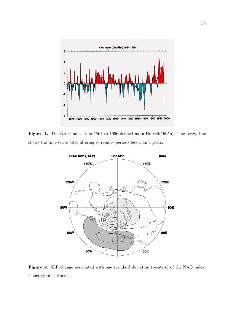
Figure 1 shows the time series of Hurrell’s NAO index from 1864-1994, and Figure

2 shows the winter SLP departure associated with one standard deviation (positive) of

the NAO index. Geostrophic balance implies that when the index is high, the westerly

winds across the North Atlantic are stronger than normal, whereas when the index is

low, the westerly winds are weaker than normal.

The observed surface temperature (SST and air temperature over land) departure

associated with one standard deviation (positive) of the NAO index is shown in Figure 3.

The seesaw in winter temperatures between western Greenland and Europe is evident,

a high NAO index (stronger than normal westerly winds) being associated with cold

winters in western Greenland and warm winters in Europe, and vica versa (van Loon

and Rogers, 1978). The importance of the NAO for understanding winter temperature

variability is clear from the analysis of Hurrell(1996). He has shown that the NAO

alone can account for 31% of the winter surface temperature variance over the northern

hemisphere north of 20oN, and that the NAO and El Nino combined can account for

44% of the winter surface temperature variance (based on 60 years of data from 1935

to 1994). The NAO is therefore important not just for winter surface temperature

variability in the North Atlantic sector, but for winter surface temperature variability

over the northern hemisphere as a whole. Indeed, it is a remarkable feature of Figure

3 that the change in winter temperature associated with the NAO extends all the way

6

across the Eurasian continent from the Atlantic to the Pacific, with the NAO apparently

having just as much influence on winter temperature in Siberia as in western Europe.

This is an indication that the NAO is not a regional North Atlantic phenomenon, but

is actually closely related to a hemispheric mode of variability known as the Arctic

Oscillation (Thompson and Wallace, 1998).

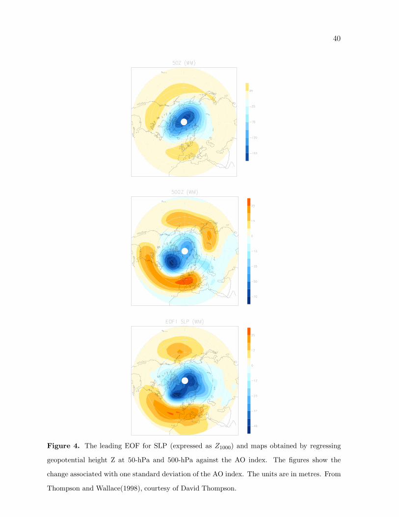
As defined by Thompson and Wallace(1998), the Arctic Oscillation (AO)

corresponds to the first EOF (Empirical Orthogonal Function) of SLP variability over

the northern hemisphere. As can be seen from Figure 4 (bottom panel), the spatial

structure of the AO corresponds closely to that associated with the NAO (Figure 2).

Thompson and Wallace(1998) find that the correlation coefficient between the principal

component time series (the AO index) and the NAO index is 0.69, and show that the

AO index is actually more strongly coupled to Eurasian winter surface air temperature

than the NAO index. It follows that while the AO and NAO are not identical, they

are certainly closely related, and the AO index may, in fact, be a better indicator of

the atmospheric mode of variability usually associated with the NAO. Accordingly, in

what follows, we shall assume that the AO and NAO correspond to the same physical

phenomenon, while bearing in mind the differences in detail. (For further discussion on

the relationship between the AO and the NAO, and also on the nature of the AO itself,

see Deser(2000) and Monahan et al.(2000).) Thompson and Wallace(1998) note that

the AO accounts for 22% of the variance in winter SLP over the northern hemisphere

poleward of 20oN (here winter is defined as November-March, and 40 years of data

are used from 1958 to 1997). They show that the AO is an equivalent barotropic

phenomenon (see Figure 4), with a strong signature in the winter stratosphere where

it accounts for 50% of the variance in the height of the 50-hPa pressure surface.

Furthermore, the geopotential height anomalies at the 50-hPa level associated with the

AO are almost five times as strong as the corresponding 1000-hPa height anomalies,

and since the spatial patterns are almost the same, it follows that the energy density

7

(the product of density and squared amplitude) is nearly the same at both 1000-hPa

and 50-hPa. This remarkable feature of the AO has led some authors to suggest that

the stratosphere may play an important role in its dynamics, as issue we shall return to

in Section 4. The work of Thompson and Wallace(1998) also makes it clear that the

variability in the AO consists of a transfer of mass in and out of the circumpolar polar

vortex. A similar mode of variability (the Antarctic Oscillation or AAO) is known to

exist in the Southern Hemisphere where the signature in the troposphere is even more

symmetric about the pole (Thompson and Wallace, 2000). It seems likely that the

bias towards the North Atlantic in the surface and middle troposphere structure of the

AO is a consequence of the land-sea contrasts in the Northern Hemisphere (Thompson

and Wallace, 1998) and presumably also the mountain ranges (e.g. The Rockies and

Greenland) that cut across the path of the tropospheric jet stream.

Let us now examine the time series of the NAO index in more detail (Figure 1).

Striking features are the low values during the period from the early 1950s to the early

1970s, relatively high values in the early part of this century, and the high values of

the last 25 years, during which time the index also shows strong decadal variability.

Caution should be exercised when interpreting these changes in the character of the

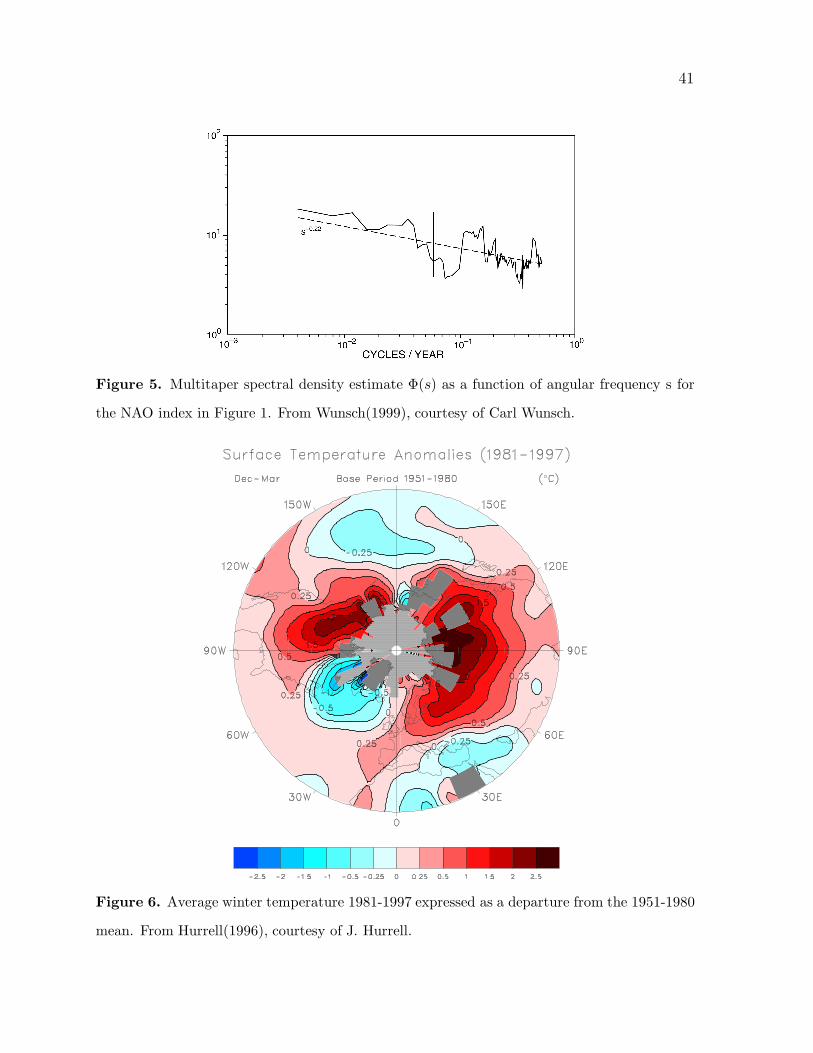
index. Figure 5 shows the estimated power density spectrum computed from Hurrell’s

time series by Wunsch(1999). This shows a weakly red spectrum, with weak structures

near periods of 2 and 8-10 years, but no particularly striking peaks. As such, the

characterisation of the NAO as an “oscillation” is misleading since its spectrum is much

more akin to that of white noise. Wunsch also shows that statistically there is no reason

to attach any significance to the variations in the character of the time series, such as

the periods of high and low index noted above, or the enhanced decadal variability in

recent years. He shows that such events are the expected behaviour of a weakly red

noise process, and need have no “cause” any more than does a sequence of rolls of dice

that produces a statistical excess of the value six. This is an issue we shall return to in

8

Section 4.

The pattern of temperature changes in the Northern Hemisphere during the period

1981-1997 has been one of warming over the continents and cooling over the oceans

(Figure 6), strongly resembling the pattern of temperature change associated with the

NAO (Figure 3). The similarity between these two patterns suggests that the recent

increase in temperature over the Northern Hemisphere is related to the positive phase of

the NAO index since the early 1980s evident from Figure 1 (Hurrell, 1996; Thompson,

Wallace and Hegerl, 2000). Some model simulations show an increasing trend in the

AO index in response to greenhouse gas forcing (Shindell et al., 1999; Fyfe et al., 1999),

leading to speculation that the recent tendency for a higher AO/NAO index might be

associated with global warming. At the present time, however, this remains speculation

(see, for example, Paeth et al., 1999).

The NAO also has an influence on storm track variability. Figure 7, taken from

Rogers(1990), shows the January mean SLP and winter (December/January/February)

storm tracks obtained by compositing months with high and low NAO index (see Rogers,

1990, for details). It is clear that the NAO has a major influence on storm tracks, with

reduced activity in the northeastern part of the North Atlantic when the index is low.

The change in the mean and eddy components of the flow between high and low

index also leads to a change in the convergence of moisture transport and is thus linked

to regional precipitation variations. Figure 8 shows evaporation minus precipitation

(E-P) computed as a residual of the atmospheric moisture budget using ECMWF

analyses for high index minus low index winters (see Hurrell, 1995b, for details). The

moisture convergence over the northern part of the British Isles and Scandinavia is

associated with wetter than normal conditions in high index years, while high index

is also associated with drier than normal conditions over parts of southern Europe,

the Mediterranean and parts of North Africa (Hurrell and van Loon, 1997). The

1981-1994 winter average precipitation anomalies, expressed as departures from the

9

1951-1980 mean, show positive anomalies over the British Isles and northern Europe,

and negative anomalies over central and southern Europe. This pattern bears a striking

resemblance to the changes in precipitation corresponding to a unit deviation of the

NAO index calculated for the winters of 1900-1994 (Hurrell and van Loon, 1997). As

with temperature, this similarity suggests that the recent precipitation anomalies over

Europe can be associated with to the upward trend of the NAO index during the past

several decades. Thompson, Wallace and Hegerl(2000) show that many climate variables

exhibit trends in the past several decades, and that a large part of the trend (although

not all) can be accounted for by the upward trend in the AO. The changing precipitation

patterns of the 1980’s and 1990’s led to reduced precipitation over the Greenland Ice

Sheet and the Alps, but enhanced precipitation over the Scandinavian mountains with

consequences for the local snow pack, and the associated skiing industry. The increased

snowfall over the Alps in recent years can, in turn, be associated with a return to low

NAO index conditions.

3. The NAO and variability in the North Atlantic Ocean

The Labrador Sea and the Greenland/Iceland/Norwegian (GIN) Seas of the North

Atlantic Ocean are two of the few places where the deep waters of the world ocean are

known to be renewed. The only other locations of any significance are the Arctic Ocean

and the Ross and Weddell Seas around Antarctica. This means that unlike the North

Pacific Ocean, the North Atlantic is an active conduit through which newly formed dense

waters spread into the rest of the global ocean. The large scale flow associated with

the spreading of newly formed dense waters is known as the thermohaline circulation

(THC). Broecker(1991) has suggested that the THC associated with North Atlantic

Deep Water forms a global ocean circulation he has termed the “Conveyor Belt”.

Associated with the “Conveyor Belt”, heat is transported northward in both the North

and South Atlantic Oceans. At 24oN, the northward heat transport has been estimated

10

as 1.2 ± 0.3 PW (Hall and Bryden, 1982) (1 PW = 1015 Watts). Almost all this heat

is released to the atmosphere over the North Atlantic north of 24oN, an amount of

heat roughly equivalent to having one 100 Watt light bulb pointing upwards on every

square meter of ocean! The heat released by the North Atlantic to the atmosphere plays

an important role in moderating the climate of western Europe and, to some extent,

Atlantic Canada. When the NAO index is high, the westerly winds penetrate more

strongly into the Eurasian continent, and the moderating influence is correspondingly

more effective than when the index is low (Figure 3).

Given the importance of the NAO/AO as a mode of variability in the overlying

atmosphere, we should not be surprised that the NAO is an important forcing for the

North Atlantic Ocean. This was recognised by Bjerknes(1964) in his now classic study

of air-sea interaction over the North Atlantic. Indeed, Bjerknes made considerable use in

his analysis of the surface pressure difference between Iceland and the Azores (an index

of the NAO). Bjerknes examined the relationship between anomalies in North Atlantic

SST and North Atlantic SLP. He suggested that on the interannual time scale, SST

anomalies are locally driven by changes in the heat flux from the atmosphere, whereas on

the decadal time scale, changes in the ocean circulation, and hence ocean heat transport

play a role. The decadal time scale is the time scale associated with oceanic advection

and baroclinic Rossby wave propagation and hence with the baroclinic adjustment

of midlatitude gyres to changing surface forcing. Bjerknes’ work has since been

updated, and his conclusions supported by Cayan(1992), Deser and Blackmon(1993),

Kushnir(1994), Battisti et al.(1995), Halliwell and Mayer(1996), Halliwell(1997, 1998),

and by the modelling work of Hakkinen(1999), Eden and Jung(2000) and Eden and

Willebrand(2000). Cayan shows a direct connection between North Atlantic SST

(NASST) anomalies and forcing by the NAO. Bjerknes’ suggestion is also consistent

with results from the GFDL coupled ocean/atmosphere model. On the interannual

time scale, NASST anomalies in the model are directly forced by surface flux variations

11

from the atmospheric model (Delworth, 1996), whereas on the interdecadal time scale,

NASST anomalies are associated with changes in the poleward heat transport associated

with fluctuations in the THC of the model (Delworth et al., 1993). On both time

scales, the important atmospheric forcing for the ocean model is closely related to the

NAO in the atmospheric model (Delworth et al., 1993; Delworth, 1996; Delworth and

Greatbatch, 2000).

Eden and Jung(2000) describe results from a North Atlantic circulation model

driven by surface flux forcing based on a monthly NAO index from 1865-1997.

These authors are the first to show conclusively that a circulation model has skill at

reproducing the observed interdecadal evolution of SST anomalies in the North Atlantic,

and to demonstrate the role played by the changing ocean circulation in that evolution.

To obtain the spatial structure of the forcing for the model, they regress the fields of

anomalous surface heat, freshwater and momentum fluxes against the NAO index for

the period 1957-1997 using NCEP/NCAR reanalysis data (Kalnay et al., 1996). The

spatial structure obtained from the regression is then multiplied by a monthly NAO

index obtained as the difference in normalised monthly mean SLP between the Azores

and Iceland (as in Rogers, 1984) for every month from 1865 to 1997. In this way,

realistic forcing fields are obtained for the model from 1865 to 1997. The skill of the

model at capturing the evolution of interdecadal SST anomalies is illustrated in Figure

9. Of particular interest is the cold anomaly that is found to the southeast of the US

in 1960-64 and subsequently spreads and intensifies northwards in both the model and

the observations. The spreading and intensification of this anomaly across 40oN takes

place in the model despite the absense of NAO-derived forcing near 40oN, and, until the

early 1980’s, in the face of forcing of the opposite sign (i.e. anomalous heating of the

ocean) north of 40oN. In the model, the evolution of this SST anomaly is driven by the

convergence of heat transport associated with the ocean circulation, and in particular

by changes in the strength of the THC and the subpolar gyre circulation. In contrast

12

to the interpretation given by Hansen and Bezdek(1996) and Sutton and Allen(1997),

advection of the SST anomalies by the mean circulation is not important in this model

(see also Visbeck et al., 1999). Eden and Jung also show that on the interdecadal time

scale, the most important contribution to the anomalous forcing of their model comes

from the surface heat flux, in agreement with the analysis of the GFDL coupled model

carried out by Delworth and Greatbatch(2000) - see Section 5. They also note that

in the subpolar gyre region of both their model and the observations, the changes in

SST lead those in the atmosphere. This is not necessarily an indication that the ocean

is driving the atmosphere, since in the model, it is a consequence of the role of ocean

dynamics in the evolution of the SST anomalies, and, in particular, of the dynamical

adjustment of the ocean model to the specified NAO-forcing.

Eden and Jung’s results show interdecadal changes in the horizontal gyre transport

of the subtropical and subpolar gyres. Bottom pressure torque, associated with the deep

circulation in the model, plays an important role in determining the transport changes.

Eden and Willebrand(2000) show an example in which changes in the transport of

the model’s subpolar gyre are driven by changes in bottom pressure torque associated

with the anomalous heat flux forcing used to drive the model, the gyre transport

lagging the heat flux forcing by about 2-3 years. There is also evidence that the

transport of the Gulf Stream undergoes changes on the interannual and interdecadal

time scales (Worthington, 1977; Greatbatch et al., 1991; Sato and Rossby, 1995). The

diagnostic calculations of Greatbatch et al.(1991) suggest that the Gulf Stream was

reduced in transport by about a third in the early 1970’s compared to the late 1950’s,

a change that is much larger than is found in Eden and Jung’s model. Ezer, Mellor

and Greatbatch(1995), using the Princeton Ocean Model, diagnosed a similar change in

transport to that found by Greatbatch et al.(1991) and were also able to show that the

model predicted changes in coastal sea level agree quite well with the observed changes

in sea level between the late 1950’s and early 1970’s. Although changes in the surface

13

wind stress play some role in leading to the model-computed changes in sea level, the

dominant influence is that of the change in the large scale ocean circulation computed

by the model. In the diagnostic models of Greatbatch et al. and Ezer et al., the change

in gyre transport is almost entirely due to the bottom pressure torque, implying a role

for the deep circulation.

The NAO can influence the THC through its influence on deep water renewal.

Deep convection, and the associated renewal of the ocean’s dense water masses, does not

occur in every year. For example, Lazier(1980) has pointed out that deep convection

did not occur in the Labrador Sea during the late 1960’s and early 1970’s, a time

when the NAO index was predominantly low (Figure 1). In fact, the occurrence of

deep convection in the Labrador Sea depends strongly on the severity of the winter in

eastern Canada, which in turn is linked to the NAO (Ikeda, 1990; Dickson et al., 1996).

When the NAO index is high, the westerly winds are stronger than normal and there

are more frequent cold, dry air outbreaks from Labrador. These cold air outbreaks cool

the surface layer of the Labrador Sea and, in late winter, can lead to strong convective

overturning, sometimes to a depth of over 2000m (Marshall and Schott, 1999). On the

other hand, when the NAO is low, the westerly winds are weaker than normal, and

outbreaks of cold, dry air from the continental interior are less frequent and less severe.

The likelihood of deep water renewal is then correspondingly reduced, as happened in

the late 1960’s. Dickson et al.(1996) point out that the influence of the NAO works in

the opposite fashion in the Greenland Sea. In particular, when the NAO index is high,

the Greenland Sea experiences less severe winter conditions than normal, in contrast

to the Labrador Sea, leading to reduced deep convective activity. The opposite is

true when the NAO index is low. In the early 1990’s, the NAO index reached record

high levels. Deep convection in the Labrador Sea penetrated to over 2000m depth,

and the newly formed Labrador Sea Water (LSW) was the freshest, coldest, and also

the densest ever observed (see Figure 10). By contrast, deep water renewal in the

14

Greenland Sea was substantially reduced at this time. The seesaw between the Labrador

and Greenland Seas is another example of the seesaw in winter temperatures between

western Greenland and Europe noted by van Loon and Rogers(1978). The NAO also

influences the production of 18oC mode water in the Sargasso Sea. When the index is

low, there are more frequent cold dry air outbreaks from the continental US, leading to

more 18oC mode water formation, the reverse being true when the index is high (see

Dickson et al.(1996) for more discussion).

It is of considerable interest to investigate the influence of changes in deep water

production on the rest of the North Atlantic. Read and Gould(1992) have traced

the influence of the shutdown in the production of LSW in the late 1960’s on the

thermohaline (subsurface) structure of the North Atlantic. Curry et al.(1998) relate

changes in the thermohaline structure to the NAO by noting the influence of the NAO

on the production of LSW, and, in turn, the influence of LSW on the thermohaline

structure (see also Sy et al., 1997). Curry et al. estimate a time scale of 6 years between

the formation of the LSW in the Labrador Sea and its appearance at Bermuda. Molinari

et al. (1999) have noted the appearance at 26oN of the anomalously cold and fresh LSW

formed during the high NAO index years of the 1980’s. Molinari et al. note that the

principal conduit between the formation region of LSW and 26oN is the Deep Western

Boundary Undercurrent. They estimate that the time taken for newly formed LSW to

reach 26oN is about 10 years.

There has also been considerable interest in the occurrence of low salinity anomalies

that propagate around the subpolar gyre of the North Atlantic. The most famous

example is the Great Salinity Anomaly (GSA) of the late 1960’s and 1970’s (Dickson

et al., 1988), but there have been other instances, as discussed by Belkin et al.(1998).

Reverdin et al.(1997) carried out an an EOF analysis on lagged time series of upper

ocean salt and heat content and found that the first EOF for salt content accounts

for 70% of the variance. This EOF corresponds to salinity anomalies that propagate

15

cyclonically around the Labrador Sea and then northeastwards to Europe on a time

scale of 5-10 years, behaviour that is very similar to that of the GSA. The principal

component time series shows strong decadal variability (although it should be noted that

only 39 years of data were available for the analysis). Reverdin et al. demonstrate the

close connection between this propagating salinity mode and a pattern of atmospheric

variability closely resembling the NAO (see Figure 17 in their paper). Like Belkin et al.,

Reverdin et al. note that the low salinity, GSA events, likely have their origin in either

the Arctic Ocean or the Canadian Arctic. Reverdin et al. point out the important role

played by the slope currents around the Labrador Sea (the West Greenland Current

and the Labrador Current) in transporting pulses of fresh water from the Arctic to the

rest of the North Atlantic. Hakkinen(1993) carried out a model study to investigate the

origin of the GSA. She concluded that the anomalous northerly winds along the east

coast of Greenland associated with the low NAO index in the 1960’s were important for

generating the GSA, confirming an hypothesis of Aagaard and Carmack(1989) that the

GSA resulted from increased export of sea-ice and freshwater from the Arctic Ocean

via Fram Strait. A slightly different hypothesis, involving an Arctic climate cycle, has

been put forward by Mysak et al.(1990). The importance of the atmospheric forcing

(and hence the NAO) for generating the interannual variability in sea-ice cover over the

Newfoundland and Labrador Shelves has been demonstrated by Ikeda et al.(1988). In

particular, severe winter conditions in Labrador, in association with the high index state

of the NAO, lead to heavy ice years. The impact of the NAO on the ocean climate of

the Newfoundland shelf has also been discussed by Myers et al.(1988).

The important role of the NAO for determining temperature variability in the North

Sea has been shown by Dippner(1997a). Heyen and Dippner(1998) show the importance

of river runoff associated with precipitation anomalies for determining salinity anomalies

in the German Bight, confirming an earlier conclusion of Schott(1966). As Heyen and

Dippner(1998) point out, although there is a clear link between the salinity anomalies

16

and the atmospheric circulation, the correlation with the NAO is weak (the SLP pattern

most closely associated with the salinity variability is similar to the Scandinavian

pattern discussed by Rogers, 1990). Dippner(1997a,b) has shown that the recruitment

of certain fish stocks in the North Sea is strongly influenced by the NAO through the

influence of the NAO on SST. For the case of cod, low SST (low NAO) favours higher

recruitment, as happened in the 1960’s. Mann and Drinkwater(1995) have argued that

the anomalous ocean conditions associated with the high NAO index in the early 1990’s

played a role in the collapse of the northern cod stock off the east coast of Newfoundland

and Labrador. The ecological impact of salinity anomalies (and hence the NAO) on

the Northwest Atlantic has also been discussed by Mertz and Myers(1994), Myers et

al.(1993) and the references therein.

4. Some thoughts on the dynamics of the NAO

As pointed out by Barnett(1985), the NAO is an internal mode of variability of

the atmospheric circulation. Indeed, low frequency (interannual and interdecadal)

variability of the NAO is found in simplified atmospheric circulation models that have

only seasonal forcing (James and James, 1989), as well as in sophisticated atmospheric

general circulation models (AGCM’s) with specified climatologically varying SST at the

lower boundary. It follows that dynamical coupling with the ocean is not necessary to

understand the basic dynamics underlying the NAO. A recent example is provided by

Limpasuvan and Hartmann(1999). These authors have analysed output from a 100 year

run of an AGCM with seasonal forcing only and demonstrate the very important role

played by the transient and stationary eddy fluxes in the maintenance of the different

phases of the AO. Limpasuvan and Hartmann(1999) compute the divergence of the

Eliassen-Palm flux and show that the eddies systematically drive the anomalous flow in

the upper troposphere in the high and low index states in the model (Figure 11). The

role of eddy fluxes in maintaining the NAO has also been noted by Hurrell(1995a) and

17

Hurrell and van Loon(1997). These authors use European Centre for Medium Range

Weather Forecasting (ECMWF) global analyses of atmospheric data to show that the

eddy flux of vorticity systematically acts to reinforce and maintain the anomalous

atmospheric circulation associated with the high NAO index state, while the eddy

flux of heat acts to damp the temperature anomalies that are being generated by

the anomalous mean flow. Derome, Brunet and Wang(2000) have analysed potential

vorticity fluxes on isentropic surfaces in the upper troposphere and find that the NAO

is essentially a free mode of the system, maintained by the eddy fluxes. All these

studies point to the conclusion that the AO (and hence the NAO) is fundamentally

an atmospheric phenomenon, and that to understand the dynamics of the AO/NAO

we must understand eddy/mean flow interaction in the atmosphere. It follows that

the AO/NAO is ultimately associated with the nonlinear transfer of energy from the

synoptic and other intraseasonal time scales to lower frequencies. For this reason,

the AO/NAO likely has a large random component in its variability, a point of view

supported by the observation of Wunsch(1999) that the spectrum of the NAO is almost

white (see Figure 5).

Although dynamic coupling with the ocean is not necessary to understand the

basic dynamics underlying the NAO, many authors have suggested that interdecadal

climate variability over the North Atlantic (and hence the NAO) may be a dynamically

coupled ocean-atmosphere phenomenon (e.g. Deser and Blackmon, 1993; Wohlleben and

Weaver, 1995; Sutton and Allen, 1997; McCartney, 1997; Curry et al., 1998; Grotzner

et al., 1998; Timmermann et al., 1998; Marshall et al, 2000). This idea is appealing

because the typical limit of predictability for the atmosphere is about three weeks. If

the large heat capacity of the ocean compared to the atmosphere can be invoked to

extend the memory of the North Atlantic ocean/atmosphere system, then it follows

that the NAO may be predictable on much longer time scales extending out to seasonal

and beyond (e.g. Griffies and Bryan, 1996). There are at least three difficulties with

18

the argument that variability in SST regulates the variability of the NAO. First there

is the controversy that surrounds the atmospheric response to North Atlantic SST

anomalies. Related to this controversy is the difficulty in interpreting the results from

AGCM’s forced by the observed time history of SST and sea-ice, as pointed out by

Bretherton and Battisti(2000), a problem that is particularly pertinent to the NAO

(see the following discussion). Thirdly there is the growing body of evidence that the

stratosphere is an important player in determining the variability of the AO (and hence

the NAO) during the winter season. We shall discuss each of these in turn, together

with the implications for AO/NAO predictability.

The controversy that surrounds the atmospheric response to midlatitude SST

anomalies, and, in particular North Atlantic SST anomalies, is nicely reviewed by

Kushnir and Held(1996) and Lau(1997). Some AGCM’s show a relatively strong

response to North Atlantic SST anomalies (e.g. Rodwell et al., 1999; Mehta et al.,

2000), while others show no response at all (e.g. Zwiers et al., 2000), and others show

a response that depends on the basic state of the atmospheric circulation (Peng et

al., 1995). (It should be noted that the statistical robustness of Peng et al.’s result is

not clear). In the studies of Rodwell et al.(1999) and Mehta et al.(2000) an ensemble

of AGCM experiments was carried out, each experiment being forced by the time

series of observed SST and sea-ice, but each started with a different initial condition.

These authors find that the NAO for the ensemble mean of the different runs is highly

correlated with the observed NAO index, the correlation being as high as 0.7 on time

scales longer than about 6 years. Bretherton and Battisti(2000; hereafter BB) have

questioned the interpretation that should be put on the results of Rodwell et al. and

Mehta et al.. They point out that the AO/NAO is an important local forcing for North

Atlantic SST. This means that even if the overlying atmosphere is sensitive to the

underlying SST, there is still the problem of predicting the SST, a problem that is

made doubly difficult when, as for the NAO, the overlying atmosphere contains a large,

19

random component that is driving the SST anomalies.

It is worth exploring Bretherton and Battisti’s work in more detail. The model

is very simple and one-dimensional (the details can be found in Barsugli and Battisti,

1998). The model is formulated in terms of temperature anomalies Ta and To for the

middle troposphere and the ocean mixed layer, respectively, and is driven by a white

noise forcing N representing the chaotic dynamics generated by the synoptic variability.

The governing equations are

dTa

dt= −aTa + bTo + N (1)

and

βdTo

dt= cTa − dTo. (2)

β represents the large heat capacity of the ocean mixed layer compared to the

atmosphere and in BB has value 40. The other parameters are a=1.12, b=0.5, c=1,

d=1.08 (note that since b 6= 0, some sensitivity of the overlying atmosphere to the SST

is allowed). The same analysis procedure is then applied to this simple coupled model

as was used by Rodwell et al. and Mehta et al. to analyse their experiments. First

a time series of the ocean temperature, T C

o, is generated using a particular realisation

of the random number generator N . (We call this the truth run). The time series

T Co is then used to drive equation (1), i.e. the atmospheric model, in an ensemble of

experiments with different realisations of N . The results in Table 1 show that this very

simple model is able to reproduce the behaviour found by Rodwell et al. and Mehta et

al., including the high correlation between the atmospheric temperature of the ensemble

mean and the atmospheric temperature in the truth run. This is true even though T Co is

generated in the truth run by random forcing from the atmosphere model. The reason

for this behaviour is that the ensemble averaging acts to filter out the noise from the

atmosphere only runs, leaving only the signal associated with the SST (that part of

the solution to (1) that arises because b 6= 0). However, because the particular time

20

series T Co is itself generated by the random forcing from the atmosphere model, there is

no predictability within the coupled system beyond that associated with the large heat

capacity of the ocean. Indeed, BB estimate that despite the excellent hindcast skill of

an atmospheric ensemble forced by observed SST’s, less than 15% of the variance in

the seasonal atmospheric (NAO) anomaly is predictable six months in advance, even

given perfect initial conditions for the midlatitude ocean state. The simple model

also explains what was a puzzling feature of Rodwell et al.’s results, namely that the

computed air/sea fluxes act to damp the SST anomalies in Rodwell et al.’s experiments,

not reinforce them, as happens in nature (see Section 3). This is also a feature of the

simple linear model and arises because in the atmosphere-only experiments, the specified

SST is a driving force for the atmosphere model and tends to lead, rather than lag, the

atmospheric temperature.

The difficulty pointed out by BB arises when the SST in the coupled system is

being driven by atmospheric variability that has a large random component. The

models of Rodwell et al. and Mehta et al. nevertheless do have some response to

the underlying SST. In BB’s model this is taken into account by the nonzero value

for b. It follows that if SST is influenced by some process other than local random

forcing from the atmosphere, dynamic coupling between the atmosphere and the ocean

might lead to some significant predictability. We have seen that on interdecadal time

scales (30 years and longer), North Atlantic SST can evolve independently of the local

forcing (Bjerknes, 1964), as recently demonstrated by Eden and Jung(2000). It is

therefore possible that some information about the future (interdecadal time scale)

atmospheric state may reside in the slow, interdecadal evolution of the ocean. The

possibility of predictive skill within the ocean on decadal time scales has been noted

by Griffies and Bryan(1996). It should be cautioned, however, that the percentage

of the atmospheric variance that might be predictable in this way may turn out to

be very small, as implied by the almost white spectrum of the NAO noted when

21

discussing Figure 5 (Wunsch, 1999). One other possibility still under investigation

is that SST in the tropical Atlantic may play a role in modulating the variability of

the AO/NAO, perhaps through the TAV. (TAV is Tropical Atlantic Variability: see

Nobre and Shukla(1996) and also the Atlantic Climate Variability Experiment (ACVE)

prospectus at http://www.ldeo.columbia.edu/ visbeck/acve/report/acve report.html.)

It is known that the atmosphere is much more sensitive to the underlying SST in the

tropics than at midlatitudes (Lau, 1997). This possibility is suggested by the work of

Robertson et al.(2000), who also find an influence of South Atlantic SST on the NAO in

their model. There is also the possibility that the atmospheric circulation may exhibit

a more significant response to the underlying SST at one time of year than at another,

as suggested by Peng et al.(1995). Czaja and Frankignoul(1999) find evidence of a

significant atmospheric response in the spring to SST anomalies in the previous winter,

and also in the early winter in response to SST anomalies the previous summer. Since

the SST anomalies persist for several months, it is possible that while the atmospheric

flow may be insensitive to the underlying SST when the anomalies are generated, there

may be greater sensitivity as the atmospheric flow evolves to a different state under the

seasonal forcing.

As noted in Section 2, the AO is an equivalent barotropic feature of the atmospheric

circulation whose energy density in winter is almost invariant with height between the

1000-hPa and 50-hPa levels (Thompson and Wallace, 1998). Indeed, fluctuations in the

strength of the wintertime stratospheric vortex are strongly linked to SLP variability in

both the northern and southern hemispheres (Thompson and Wallace, 2000). Baldwin et

al.(1994), Perlwitz and Graf(1995), Cheng and Dunkerton(1995), Kitoh et al.(1996) and

Kodera et al.(1996) have all documented coupling between the the winter stratospheric

polar vortex and its tropospheric counterpart. This suggests a possible role for the

stratosphere in modulating the AO/NAO. Recently, Baldwin and Dunkerton(1999) have

shown that AO anomalies during wintertime often first appear in the stratosphere near

22

the 10-hPa level and then propagate downward into the troposphere on a time scale of

weeks (see Figure 12). They show that the midwinter correlation between the 90 day

low pass filtered 10 hPa and 1000 hPa AO-anomalies exceeds 0.65 when the surface

anomaly time series is lagged by about three weeks. It should be possible, therefore,

to use information from the stratosphere to improve prediction of the AO/NAO in

the troposphere one month ahead during the winter season, with the implication that

models used for long-range prediction may require a detailed representation of the

stratosphere. In Section 2, it was noted that the stratosphere may play a role in

explaining the increasing trend of the AO/AAO that is found in some recent model

experiments under greenhouse gas forcing (Shindell et al., 1999; Fyfe et al., 1999; Paeth

et al., 1999). Clearly, more research is required to unravel the dynamic link between the

stratosphere and AO/NAO, a topic that is of interest on a wide range of time scales.

The importance of wave mean flow interaction for the dynamics of the AO/NAO

suggests a link between the NAO and the frequency of atmospheric blocking. A

blocking pattern, such as shown in Figure 13, projects negatively on the NAO index

(the pressure difference between Iceland and the Azores) and the recurrence of such

events throughout a season would lead to a low NAO index. Hurrell(1996) notes that

the 1960’s, when the NAO index was low, was a period of frequent wintertime blocking

over the North Atlantic. Huang et al.(2000) have shown that both the frequency and

lifetime of blocking events in the North Atlantic region is related to the phase of the

NAO, with more frequent, longer lasting blocks when the index is low. Vautard(1990)

has also noted a link between blocking over Greenland (his Greenland Anticyclone

weather regime) and the NAO. What is not clear is whether the blocks are playing a role

in causing periods of low index or whether they are merely a symptom of the weakened

polar vortex associated with low index. Blocking events in the troposphere are known

to be linked with stratospheric sudden warmings (Andrews et al., 1987; Quiroz, 1986)

suggesting, once again, a dynamical link between the NAO and stratosphere.

23

5. The “Null Hypothesis” for North Atlantic

interannual/interdecadal variability

The discussion in Section 4 suggests that dynamical coupling between the

atmosphere and ocean is not strong over the North Atlantic, at least on time scales

out to interannual and interdecadal. It follows that the simplest possible interpretation

for interannual to interdecadal variability in the North Atlantic climate system is

the “Null Hypothesis”, according to which the midlatitude ocean responds passively

to the overlying atmospheric variability, and, in particular, does not feed back and

dynamically influence the overlying atmospheric circulation. (For more discussion of

the “Null Hypothesis” see the Atlantic Climate Variability Experiment prospectus at

http://www.ldeo.columbia.edu/ visbeck/acve/report/acve report.html.) This view is

consistent with Dickson et al.(1996) who state “we see strong evidence of a direct impact

of the shifting atmospheric circulation on the ocean; while this certainly does not rule

out either feedbacks from anomalous ice and SST conditions on the atmosphere, or

autonomous oscillations of the ocean’s overturning circulation, it does tend to minimize

them”.

Delworth and Greatbatch(2000) describe an application of the “Null Hypothesis”

to understand the interdecadal variability in the Atlantic sector of the GFDL coupled

ocean/atmosphere model (Delworth et al., 1993). Figure 14 shows the times series of the

strength of the thermohaline circulation (THC) in the coupled model. To understand

the variability, we begin by noting that the ocean component of the coupled model

does not support its own self-sustained interdecadal variability in the Atlantic sector

(Greatbatch et al., 1997). This is because the realistic bottom topography acts as a

strong damping (Winton, 1997), and contrasts with the self-sustained interdecadal

variability found in the flat-bottomed models of Weaver and Sarachik(1991), Greatbatch

and Zhang(1995) and many similar studies. Rather, the THC variability in the coupled

24

model is sustained by the variable atmospheric forcing, as in the box model of Griffies

and Tziperman(1995). Delworth and Greatbatch(2000) show that the surface heat flux

is the dominant term (relative to the fresh water and momentum fluxes) in driving

the THC variability (similar to the finding of Eden and Jung, 2000) and also that

the interdecadal THC variability in the coupled model is driven by the low frequency

portion of the spectrum of atmospheric flux forcing (time scales of 20 years and longer).

Analyses also reveal that the THC fluctuations are driven by a spatial pattern of surface

heat flux variations that bears a strong resemblance to the North Atlantic Oscillation

(Figure 15).

To assess the importance of dynamic coupling between the atmosphere and ocean

models, the results of two experiments are described in which the coupling is suppressed

(Figure 16). In RANDOM, the ocean component of the coupled model is driven by

annual mean surface fluxes taken from the coupled model but randomly rearranged

in time, and in ATMOS, the ocean model is driven by a time series of annual mean

fluxes taken from the atmospheric component of the coupled model run with specified

seasonally varying SST and sea-ice. Both model runs show that significant interdecadal

variability in the THC can be generated by low frequency atmospheric forcing that does

not rely on dynamical coupling with the ocean. In ATMOS, the interdecadal variability

in the THC is being driven entirely by interdecadal variability generated internally

within the atmospheric model. In RANDOM, the flux forcing has a white spectrum and

is varying completely independently of the underlying SST. The amplitude of the THC

variability in RANDOM and ATMOS is nevertheless reduced compared to that in the

coupled model, particularly in ATMOS (the standard deviation of the THC variability

in the coupled model is 0.98 Sv, compared with 0.77 Sv in RANDOM and 0.47 Sv in

ATMOS). Delworth and Greatbatch(2000) argue that this is because thermodynamic

coupling (as well as dynamic coupling) is suppressed in ATMOS and RANDOM.

Thermodynamic coupling is important in the deep convection region where heat can

25

be stored in the ocean during periods of reduced convection and then released when

convection becomes active again, a process that leads to enhanced heat flux variability

in the deep convection region. The absense of any influence from deep convection is very

evident in ATMOS and can be seen by comparing the three panels in Figure 15. (In

the model, deep convection takes place primarily to the south of Greenland.) Delworth

and Greatbatch(2000) conclude that there is no evidence that the THC variability

in the coupled model is part of a dynamically coupled mode of the atmosphere and

ocean models. We believe, therefore, that the THC variability in the GFDL model is

consistent with the “Null Hypothesis”.

6. Summary and Conclusions

The NAO is the most important mode of variability in the atmospheric circulation

over the North Atlantic, with considerable influence on winter temperature throughout

the Eurasian continent and eastern North America (Figure 3). The NAO is closely

related to the AO which, as pointed out by Thompson and Wallace(1998), is a

hemispheric mode of variability that extends throughout the depth of the troposphere

and up into the winter stratosphere. Indeed, there is growing evidence that the

stratosphere plays an important role in winter AO/NAO variability (Baldwin and

Dunkerton, 1999) and may also be implicated in the upward trend of the AO index that

is a feature of some model simulations that include greenhouse gas forcing (Shindell

et al., 1999; Fyfe et al., 2000; Paeth et al., 1999). The AO/NAO is also an important

forcing for the North Atlantic Ocean (Section 3). AO/NAO driving of North Atlantic

SST anomalies is implicit in the classic study of Bjerknes(1964), and reiterated by

Cayan(1992) and many subsequent studies. Curry et al.(1998) point out that the

signature of the NAO is felt throughout the surface and subsurface waters of the North

Atlantic thermocline, and recent modelling studies (Hakkinen, 1999; Eden and Jung,

2000; Eden and Willebrand, 2000; Delworth and Greatbatch, 2000) emphasise the

26

importance of the AO/NAO for driving circulation changes in the North Atlantic, in

particular the thermohaline overturning circulation (THC).

Section 4 provided some discussion on the dynamics of the NAO. It was emphasised

that the AO/NAO is an internal mode of variability of the atmospheric circulation

driven by eddy/mean flow interaction (e.g. Limpasuvan and Hartmann, 1999), and

that dynamical coupling with the ocean is probably weak. Recent studies by Rodwell

et al.(1999) and Mehta et al.(2000) have used an ensemble of atmospheric general

circulation model (AGCM) experiments, driven by the observed time series of SST and

sea-ice, to reproduce the observed evolution of the NAO, apparently holding out the

prospect of predicting the NAO several years in advance. Bretherton and Battisti(2000)

have questioned this interpretation. They point out that to predict the NAO, one must

first predict the SST and sea-ice, a problem that is very difficult when, as for the NAO,

the atmosphere contains a large random component that is itself an important local

forcing for SST and sea-ice. The difficulty pointed out by Bretherton and Battisti(2000)

can be circumvented when some process other than local atmospheric forcing is driving

the SST, an example being changes in oceanic heat transport (see Figure 9 and the

discussion thereon). On the other hand, the spectrum of the winter NAO index (Figure

5) is only weakly red, with no striking peaks (Wunsch, 1999), suggesting that even on

the interdecadal time scale, there is little hope for prediction of the NAO, a conclusion

that, nevertheless, would benefit from further study using coupled ocean/atmosphere

models. More exciting from the predictability point of view is the possibility, suggested

by the study of Baldwin and Dunkerton(1999) (see Figure 12), that information in

the winter stratosphere can be used to provide information on the likely phase of

the AO/NAO in the lower troposphere one month ahead. The relationship between

the NAO and quasi-stationary regimes of the atmospheric circulation (Vautard, 1990;

Monahan et al., 2000) also requires further investigation. Sometimes the atmospheric

circulation remains close to one of these regimes for extended periods, exceeding the

27

typical three week limit of predictability. It follows that understanding these regimes

and transitions between them could prove helpful for improving prediction one season

ahead.

Acknowledgments. Funding from NSERC, AES and the Canadian Institute for Climate

Studies is gratefully acknowledged. I am grateful to my friends and colleagues George Boer,

Gilbert Brunet, Kirk Bryan, Allyn Clarke, Tom Delworth, Jacques Derome, Bernard Dugas,

John Fyfe, Nick Hall, Peter Jones, John Lazier, Charles Lin, David Marshall, Lionel Pandolfo,

Hal Ritchie, Ian Rutherford, Fritz Schott, Ted Shephard, Keith Thompson, Andrew Weaver,

Jurgen Willebrand, Ric Williams, Dan Wright and Francis Zwiers for helpful discussions

over the years that have helped shape my understanding of the NAO and North Atlantic

climate variability. I am also grateful to Mark Baldwin, Joachim Dippner, Carsten Eden and

Amir Shabbar for making their papers available to me. Thanks also to Mark Baldwin, Tom

Delworth, Carsten Eden, Jim Hurrell, Var Limpasuvan and David Thompson for providing

postscript files of figures used in this article.

28

References

Aagaard K,Carmack EC(1989) The role of sea-ice and other freshwater in the Arctic

circulation. J Geophys Res 94:14485-14498

Andrews DG,Holton JR,Leovy CB(1987) Middle Atmosphere Dynamics. Academic Press, 489

pp.

Appenzeller C,Stocker TF,Anklin M(1998) North Atlantic Oscillation dynamics recorded in

Greenland ice cores. Science 282:446-449

Baldwin MP,Cheng X,Dunkerton TJ(1994) Observed correlations between winter-mean

tropospheric and stratospheric circulation anomalies. Geophys Res Lett 21:1141-1144

Baldwin MP,Dunkerton TJ(1999) Propagation of the Arctic Oscillation from the stratosphere

to the troposphere. J Geophys Res 104:30937-30946

Barnett TP(1985) Variations in near-global sea level pressure. J Atmos Sci 42:478-501

Barnston AG, Livezey RE(1987) Classification, seasonality and persistence of low frequency

atmospheric circulation patterns. Mon Wea Rev 115:1083-1126

Barsugli JJ,Battisti DS(1998) The basic effects of atmosphere-ocean thermal coupling on

midlatitude variability. J Atmos Sci 55:477-493

Battisti DS,Bhatt US,Alexander MA(1995) A modelling study of the interannual variability in

the wintertime North Atlantic Ocean. J Climate 8:3067-3083

Belkin IM,Levitus S,Antonov J,Malmberg S-A(1998) “Great Salinity Anomalies” in the North

Atlantic. Prog Oceanogr 41:1-68

Bjerknes J(1964) Atlantic air-sea interaction. Adv Geophys 10:1-82

Bretherton CS,Battisti DS(2000) An interpretation of the results from atmospheric general

circulation models forced by the time history of the observed sea surface temperature

distribution. Geophys Res Lett 27:767-770

Broecker WS(1991) The great ocean conveyor. Oceanography 4:79-89

Cayan DR(1992) Latent and sensible heat flux anomalies over the northern oceans: Driving

the sea surface temperature. J Phys Oceanogr 22:859-881

Cheng X,Dunkerton TJ(1995) Orthogonal rotation of spatial patterns derived from singular

29

value decomposition analysis. J Climate 8:2631-2643

Cook ER,D’Arrigo RD,Briffa KR(1998) The North Atlantic Oscillation and its expression in

circum-Atlantic tree-ring chronologies from North America and Europe. The Holecene

8:9-17

Cullen H, D’Arrigo R,Cook E,Mann ME(2000) Multiproxy reconstructions of the North

Atlantic Oscillation. Paleoceanography submitted

Curry RG,McCartney MS,Joyce TM(1998) Oceanic transport of subpolar climate signals to

mid-depth subtropical waters. Nature 391:575-577

Czaja A,Frankignoul C(1999) Influence of the North Atlantic SST on the atmospheric

circulation. Geophys Res Lett 26:2969-2972

Delworth TL(1996) North Atlantic interannual variability in a coupled ocean-atmosphere

model. J Climate 9:2356-2375

Delworth TL,Greatbatch RJ(2000) Multidecadal thermohaline circulation variability driven

by atmospheric surface flux forcing. J Climate 13:1481-1495

Delworth TL,Manabe S,Stouffer RJ(1993) Interdecadal variations of the thermohaline

circulation in a coupled ocean-atmosphere model. J Climate 6:1993-2011.

Derome J,G Brunet,Y Wang(2000) On the potential vorticity balance on an isentropic surface

during normal and anomalous winters. Mon Wea Rev submitted

Deser C(2000) A note on the teleconnectivity of the “Arctic Oscillation”. Geophys Res Lett

27:779-782

Deser C,Blackmon ML(1993) Surface climate variations over the North Atlantic Ocean during

winter: 1900-1989. J Climate 6:1743-1753

Dickson RR,Lazier J,Meincke J,Rhines P,Swift J(1996) Long-term coordinated changes in the

convective activity of the North Atlantic. Prog Oceanogr 38:214-295

Dickson RR,Meinke J,Malmberg S-A, Lee AJ(1988) The “Great Salinity Anomaly” in the

Northern North Atlantic, 1968-1982. Prog Oceanogr 20:103-151

Dippner, JW(1997a) SST anomalies in the North Sea in relation to the North Atlantic

Oscillation and the influence on the theoretical spawning time of fish. Dtsch Hydrogr Z

49:267-275

30

Dippner, JW(1997b) Recruitment success of different fish stocks in the North Sea in relation

to climate variability. Dtsch Hydrogr Z 49:277-293

Eden C,Jung T(2000) North Atlantic interdecadal variability: Oceanic response to the North

Atlantic Oscillation (1865-1997). J Climate submitted

Eden C,Willebrand J(2000) Mechanism of interannual to decadal variability of the North

Atlantic circulation. J Climate submitted

Ezer T,Mellor GL,Greatbatch RJ(1995) On the interpentadal variability of the North Atlantic

Ocean: Model simulated changes in transport, meridional heat flux and coastal sea level

between 1955-59 and 1970-1974. J Geophy Res 100:10,559-10,566

Fyfe JC,Boer GJ,Flato GM(1999) The Arctic and Antarctic Oscillations and their projected

changes under global warming. Geophys Res Lett 26:1606-1604

Greatbatch RJ,Fanning AF,Goulding A,Levitus S(1991) A diagnosis of interpentadal

circulation changes in the North Atlantic. J Geophys Res 96:22009-22024

Greatbatch RJ,Peterson KA,Roth H(1997) Interdecadal variability in a coarse resolution model

with North Atlantic bottom topography. Department of Oceanography, Dalhousie

University, Halifax, Nova Scotia, Canada.

Greatbatch RJ,Zhang S(1995) An interdecadal oscillation in an idealised ocean basin forced

by constant heat flux. J Climate 8:81-91.

Griffies S,Bryan K(1996) Predictability of North Atlantic multidecadal climate variability.

Science 275:181-184

Griffies S,Tziperman E(1995) A linear thermohaline oscillator driven by stochastic atmospheric

forcing. J Climate 8:2440-2453

Grotzner A,Latif M,Barnett TP(1998) A decadal climate cycle in the North Atlantic Ocean as

simulated by the ECHO coupled model. J Climate 11:831-847

Hakkinen S(1993) An Arctic source for the Great Salinity Anomaly:A simulation of the Arctic

ice-ocean system for 1955-1975. J Geophys Res 98:16397-16410

Hakkinen S(1999) Variability of the simulated meridional heat transport in the North Atlantic

for the period 1951-1993. J Geophys Res 104:10,991-11,007

Hall MM,Bryden H(1982) Direct estimates and mechanisms of ocean heat transport. Deep

31

Sea Res Part A 29:339-359

Halliwell GR(1997) Decadal and multidecadal North Atlantic SST anomalies driven by

standing and propagating basin-scale atmospheric anomalies. J Climate 10:2405-2411

Halliwell GR(1998) Simulation of North Atlantic decadal/multidecadal winter SST anomalies

driven by basin-scale atmospheric circulation anomalies. J Phys Oceanogr 28:5-21

Halliwell GR,Mayer DA(1996) Frequency response properties of forced climate SST anomaly

variability in the North Atlantic. J Climate 9:3575-3587

Hansen DV,Bezdek H(1996) On the nature of decadal anomalies in North Atlantic sea surface

temperature. J Geophys Res 101:8749-8758

Heyen H,Dippner JW(1998) Salinity variability in the German Bight in relation to climate

variability. Tellus 50A:545-556

Huang J,Shabbar A,Higuchi K(2000) The relationship between the wintertime North Atlantic

Oscillation and blocking episodes in the North Atlantic. Int J Climatol submitted

Hurrell JW(1995a) Transient eddy forcing of the rotational flow during northern winter. J

Atmos Sci 52:2286-2301

Hurrell JW(1995b) Decadal trends in the North Atlantic Oscillation: Regional temperatures

and precipitation. Science 269:676-679

Hurrell JW(1996) Influence of variations in extratropical wintertime teleconnections on

Northern Hemisphere temperature. Geophys Res Lett 23:665-668

Hurrell JW,van Loon H(1997) Decadal variations in climate associated with the North Atlantic

Oscillation. Climate Change 36:301-326

Ikeda M(1990) Decadal oscillations of the air-ice-ocean system in the Northern hemisphere.

Atmos.-Ocean 28:106-139

Ikeda M,Symonds G,Yao T(1988) Simulated fluctuations in annual Labrador Sea ice cover.

Atmos-Ocean 26:16-39

James IN, James PM(1989) Ultra-low-frequency variability in a simple atmospheric circulation

model. Nature 342:53-55

Kalnay E, et al.(1996) The NCEP/NCAR 40 year reanalysis project. Bull Amer Met Soc

77:437-471

32

Kitoh A,Koide H,Kodera K,Yukimoto S,Noda A(1996) Interannual variability in the

stratospheric-tropospheric circulation in a coupled ocean-atmosphere GCM. Geophys.

Res Lett 23:535-546

Kodera K,Chiba M,Koide H,Kitoh A,Nikaidou Y(1996) Interannual variability of the winter

stratosphere and troposphere in the Northern hemisphere. J Met Soc Japan 74:365-382

Kushnir Y(1994) Interdecadal variations in North Atlantic sea surface temperature and

associated atmospheric conditions. J Climate 7:141-157

Kushnir Y(1999) Europe’s winter prospects. Nature 398:289-291

Kushnir Y,Held IM(1995) Equilibrium atmospheric response to North Atlantic SST anomalies.

J Climate 9:1208-1220.

Lau N-C(1997) Interactions between global SST anomalies and the midlatitude atmospheric

circulation. Bull Amer Met Soc 78:21-33

Lazier JRN(1980) Oceanic conditions at Ocean Weather Ship Bravo, 1964-1974. Atmos-Ocean,

18:227-238

Limpasuvan V,Hartmann DL(1999) Eddies and the annular modes of climate variability.

Geophys Res Lett 26:3133-3136

Loewe F(1937) A period of warm winters in western Greenland and the temperature seesaw

between western Greenland and central Europe. Quart J Roy Met Soc 63:365-372

Loewe F(1966) The temperature seesaw between western Greenland and Europe. Weather

21:241-246

Luterbacher J,Schmutz C,Gyalistras D, Xoplaki E(1999) Reconstruction of monthly NAO and

EU indices. Geophys Res Lett 26:2745-2748

Mann KH,Drinkwater K(1994) Environmental influences on fish and shellfish production in

the Northwest Atlantic. Environ Rev 2:16-32

Marshall J,Johnson H,Goodman J(2000) A study of the interaction of the North Atlantic

Oscillation with the ocean circulation. J Climate submitted

Marshall J, Schott F(1999) Open ocean deep convection: observations, models and theory.

Rev of Geophysics 37:1-64

McCartney M(1997) Is the ocean at the helm? Nature 388:521-522

33

Mehta VM,Suarez MJ,Manganello J,Delworth TL(2000) Oceanic influence on the North

Atlantic Oscillation and associated northern hemisphere climate variations:1959-1993.

Geophys Res Lett 27:121-124

Meinhardus W(1898) Uber einige meteorologische Beziehungen zwischen dem Nordatlantischen

Ozean und Europa im Winterhalbjahr. Meteor Z 15:85-105

Mertz G,Myers RA(1994) The ecological impact of the Great Salinity Anomaly in the northern

North-west Atlantic. Fish Oceanogr 3:1-14

Molinari RL,Fine RA,Wilson WD,Curry RG,Abell J,McCartney M(1998) The arrival of

recently formed Labrador Sea Water in the Deep Western Boundary Current at 26.5oN.

Geophys Res Lett 25:2249-2252

Monahan AH,Fyfe JC,Flato GM(2000) A regime view of northern hemisphere atmospheric

variability and change under global warming. Geophys Res Lett, submitted.

Mysak LA,Manak DK,Marsden RF(1990) Sea-ice anomalies observed in the Greenland and

Labrador Seas during 1901-1984 and their relation to an interdecadal Arctic climate

cycle. Climate Dynamics 5: 111-133

Myers RA,Akenhead S,Drinkwater KF(1988) The North Atlantic Oscillation and the ocean

climate of the Newfoundland shelf. NAFO SCR Doc 88/65, 22pp

Myers RA,Drinkwater KF,Barrowman NJ,Baird JW(1993) Salinity and recruitment of Atlantic

cod(Gadus morhua) in the Newfoundland region. Can J Fish Aquat Sci 50:1599-1609

Nobre P,Shukla J(1996) Variations of sea surface temperature, wind stress, and rainfall over

the tropical Atlantic and South America. J Climate 9:2464-2479

Paeth H,Hense A,Glowienka-Hense R,Voss R,Cubasch U(1999) The North Atlantic Oscillation

as an indicator for greenhouse-gas induced regional climate change. Clim Dyn

15:953-960

Peng S,Mysak LA,Ritchie H,Derome J,Dugas B(1995) The difference between early and

midwinter atmospheric responses to sea surface temperature anomalies in the Northwest

Atlantic. J Climate 8:137-157

Perlwitz J,Graf H-F(1995) The statistical connection between tropospheric and stratospheric

circulation of the Northern Hemisphere in winter. J Climate 8:2281-2295

34

Quiroz RS(1986) The association of stratospheric warmings and tropospheric blocking. J

Geophys Res 91:5277-5285

Read JF,Gould WJ(1992) Cooling and freshening of the subpolar North Atlantic Ocean since

the 1960’s. Nature 360: 55-57

Reverdin G,Cayan D,Kushnir Y(1997) Decadal variability of hydrography in the upper

northern North Atlantic in 1948-1990. J Geophys Res 102:8505-8532

Robertson AW,Mechoso CR,Kim Y-J(2000) The influence of Atlantic sea surface temperature

anomalies on the North Atlantic Oscillation. J Climate 13:122-138

Rodwell MJ,Rowell DP,Folland CK(1999)Oceanic forcing of the wintertime North Atlantic

Oscillation and European climate. Nature 398:320-323

Rogers JC(1984) The association between the North Atlantic Oscillation and the Southern

Oscillation in the Northern Hemisphere. Mon Wea Rev 112:1999-2015

Rogers JC(1990) Patterns of low frequency monthly sea level pressure variability (1899-1996)

and associated wave cyclone frequencies. J Climate 3:1364-1379

Rogers JC,van Loon H(1979) The seesaw in winter temperatures between Greenland and

northern Europe. Part II:Some oceanic and atmospheric effects at middle and high

latitudes. Mon Wea Rev 107:509-519

Sato O,Rossby T(1995) Seasonal and secular variations in dynamic height anomaly and

transport of the Gulf Stream. Deep Sea Res 42:149-164

Shindell DT,Miller RL,Schmidt GA,Pandolfo L(1999) Simulation of recent northern climate

trends by greenhouse-gas forcing. Nature 399:452-455

Schott F(1966) Der Oberflachensalzgehalt in der Nordsee. Dtsch Hydrogr Z (suppl A9):1-58

Shutts GJ(1986) A case study of eddy forcing during an Atlantic blocking episode. Adv

Geophys 29:135-162

Stockton C, Glueck M(1999) Long-term variability of the North Atlantic Oscillation.

In:American Meteorological Society 10th Symposium on Global Change Studies, Dallas

Texas, pp.290-293

Sutton RT, Allen MR(1997) Decadal predictability of North Atlantic sea surface temperature

and climate. Nature 388:563-567

35

Sy A,Rhein M,Lazier JRN,Koltermann KP,Meincke J,Putzka A,Bersch M(1997) Surprisingly

rapid spreading of newly formed intermediate waters across the North Atlantic Ocean.

Nature 386:675-679

Thompson DWJ,Wallace JM(1998) The Arctic Oscillation signature in wintertime geopotential

height and temperature fields. Geophys Res Lett 25:1297-1300

Thompson DWJ,Wallace JM(2000) Annular modes in the extratropical circulation. Part

I:Month to month variability. J Climate 13:1000-1016

Thompson DWJ,Wallace JM,Hegerl GC(2000) Annular modes in the extratropical ciruclation.

Part II:Trends. J Climate 13:1018-1036

Timmermann A,Latif M,Voss R,Grotzner A(1998) Northern hemispheric interdecadal

variability: A coupled air-sea mode. J Climate 11:1906-1931.

van Loon H,Rogers JC(1978) The seesaw in winter temperatures between Greenland and

northern Europe. Part I:General description. Mon Wea Rev 106:296-310

Vautard R(1990) Multiple weather regimes over the North Atlantic: Analysis of precursors

and successors. Mon Wea Rev 118:2056-2081

Visbeck M,Cullen H, Krahmann G,Naik N(1998) An ocean model’s response to North Atlantic

Oscillation-like wind forcing. Geophys Res Lett 25:4521-4524

Wallace JM,Gutzler DS(1981) Teleconnections in the geopotential height field during the

northern hemisphere winter. Mon Wea Rev 109:784-812

Walker GT(1924) Correlations in seasonal variations of weather IX. Mem Ind Meteor Dept

24:275-332

Walker GT,Bliss EW(1932) World weather V. Mem Roy Meteor Soc 4:53-84

Weaver AJ,Sarachik ES(1991) Evidence for Decadal Variability in an ocean general circulation

model: An advective mechanism. Atmosphere-Ocean 29:197-231.

Winton M(1997) The damping effect of bottom topography on internal decadal-scale

oscillations of the thermohaline circulation. J Phys Oceanogr 26:289-304

Wohlleben TMH, Weaver AJ(1995) Interdecadal climate variability in the subpolar North

Atlantic. Climate Dynamics 11:459-467

Worthington LV(1977) The intensification of the Gulf Stream after the winter of 1976-77.

36

Nature 270:415-417

Wunsch C(1999) The interpretation of short climate records, with comments on the North

Atlantic and Southern Oscillations. Bull Amer Met Soc 80:245-255

Zwiers FW,Wang XL,Sheng J(2000) Effects of specifying bottom boundary conditions in an

ensemble of atmospheric GCM simulations. J Geophys Res 105:7295-7315

This manuscript was prepared with the AGU LATEX macros v3.1.

37

Table 1. Simulated NAO variability given specified SST in two AGCM studies and the

Bretherton and Battisti(BB) model.

Experiment Na SeasonalbRd Low Freq.cRd ARe

Rodwell et al. 6 0.21 / 0.41 0.43 / 0.74 0.39

Mehta et al. 16 0.17 / 0.43 0.28 / 0.75 0.50

BB Model 16 0.18 / 0.45 0.45 / 0.80 0.41

aThe number of AGCM realizations in the ensemble

bSeasonal variability is loosely defined as the 3-month winter average for Rodwell et al.(1999),

the one month average for Mehta et al.(2000), and 3 months for the BB model.

c‘Low Freq.’ refers to time series low-pass filtered to retain periods greater than 6.5 years.

dCorrelation coefficients are between the simulated and observed NAO index (AGCMs) or

atmospheric temperature anomaly (BB model). The first value is the average for one

atmospheric realization, and the second value is for the ensemble mean prediction.

eRatio between standard deviation of low-pass atmospheric variability in the model to that

observed.

38

Figure 1. The NAO index from 1864 to 1996 defined as in Hurrell(1995b). The heavy line

shows the time series after filtering to remove periods less than 4 years.

Figure 2. SLP change associated with one standard deviation (positive) of the NAO index.

Courtesy of J. Hurrell.

39

Figure 3. Surface temperature change associated with one standard deviation (positive) of

the NAO index. From Hurrell(1996), courtesy of J. Hurrell.

40

Figure 4. The leading EOF for SLP (expressed as Z1000) and maps obtained by regressing

geopotential height Z at 50-hPa and 500-hPa against the AO index. The figures show the

change associated with one standard deviation of the AO index. The units are in metres. From

Thompson and Wallace(1998), courtesy of David Thompson.

41

Figure 5. Multitaper spectral density estimate Φ(s) as a function of angular frequency s for

the NAO index in Figure 1. From Wunsch(1999), courtesy of Carl Wunsch.

Figure 6. Average winter temperature 1981-1997 expressed as a departure from the 1951-1980

mean. From Hurrell(1996), courtesy of J. Hurrell.

42

��������������������������������������������������������������������������������������������������������������������������������������������������������������������������������������������������������������������������������������������������������������������������������������������������������������������������������������������������������������������������������������������������������������������������������������������������������������������������������������������������������������������

Figure 7. Top panels: The January mean SLP (hPa) for years between 1899 and 1986 with

NAO index greater than or less than one standard deviation from the mean. Bottom panels:

Isopleths of the frequency of wave cyclones per 5o latitude x 5o longitude tessarae for the nine

winter months 1957-86 with the highest (left panel) and lowest (right panel) NAO index. From

Rogers(1990).

Figure 8. Evaporation minus precipitation for high NAO minus low NAO index, computed

as the residual of the atmospheric moisture budget using ECMWF global analyses. See

Hurrell(1995b) for details. Courtesy of J. Hurrell.

43

Figure 9. Interdecadal evolution of observed and modelled winter SST anomalies (oC) for

pentads from 1960-64 to 1980-84, and the NAO-related interdecadal heat flux (Wm2) and

near surface wind (ms−1) fields that force the model. From Eden and Jung(2000), courtesy of

Carsten Eden.

44

Figure 10. The time series of observed potential temperature (top panel) and salinity (bottom

panel) in the Labrador Sea. Note the warming of the subsurface water in the 1960’s when

deep convection was suppressed, and the unprecedented cold and fresh water of the 1990’s

associated with the high NAO index of those years. Courtesy of Igor Yashayaev. (Extracted

from http://dfomr.mar.dfo-mpo.gc.ca/science/ocean/woce/labsea/labsea poster.html).

45

SAM NAM

80˚S 60˚S 40˚S 20˚S

Total Eddy

Synoptic Waves

Stationary Waves

20˚N 40˚N 60˚N 80˚N

200

400

600

800

1000

PR

ESS

UR

E (

hPa)

200

400

600

800

1000

200

400

600

800

1000

200

400

600

800

1000

Figure 11. Top panels: Cross section of the zonal mean zonal wind regressed onto the SAM

and NAM index (SAM/NAM is the Southern/Northern Angular Mode, that is the AAO and

AO, respectively). The contour interval is 0.4 ms−1 per standard deviation of the index. Also

shown as vectors is the corresponding zonal mean vertical and meridional winds. Other panels:

Composite difference of the EP flux divergence contoured every 0.5 ms−1day−1. Easterly

acceleration is shaded. Arrows indicate composite EP vector difference. All figures use output

from the GFDL model. Taken from Limpasuvan and Hartmann(1999) where the details of the

calculation can be found. Courtesy of V. Limpasuvan.

46

10

100

1000

hPa

1958 1959 1960 1961 1962

C C C C

10

100

1000

hPa

1963 1964 1965 1966 1967

C C C C

10

100

1000

hPa

1968 1969 1970 1971 1972

C C

10

100

1000

hPa

1973 1974 1975 1976 1977

C C C C

10

100

1000

hPa

1978 1979 1980 1981 1982

C C C C

10

100

1000

hPa

1983 1984 1985 1986 1987

C C

10

100

1000

hPa

1988 1989 1990 1991 1992

10

100

1000

hPa

1993 1994 1995 1996 1997

C C

Figure 12. The evolution of the 90 day low-pass filtered projection of geopotential height

on the AO computed from NCEP/NCAR reanalysis data. Red/blue shading indicates a

weakened/strengthened circumpolar vortex, respectively, and red tick marks indicate major

stratopheric warmings. From Baldwin and Dunkerton(1999) where the details of the calculation

can be found. Note the tendency for events to propagate downward on a time scale of weeks.

Courtesy of Mark Baldwin.

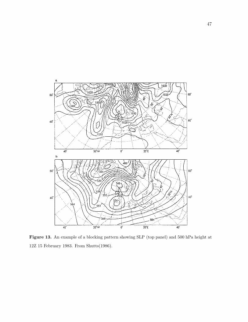
47

��������������������������������������������������������������������������������������������������������������������������������������������������������������������������������������������������������������������������������������������������������������������������������������������������������������������������������������������������������������������������������������������������������������������������������������������������������������������������������������������������������������������

Figure 13. An example of a blocking pattern showing SLP (top panel) and 500 hPa height at

12Z 15 February 1983. From Shutts(1986).

48

1000 1100 1200 1300 1400 1500 1600 1700 1800 1900 2000Year

11

12

13

14

15

16

17

Sve

rdru

ps

�

.01�

.02� .03� .05� .1� .2� .3� .5�.005.1.2.5125

102050

100 1050 20 5� 2200� 33 3.3

Frequency (cycles yr-1)

Spec

tral

Den

sity

(b)

Period (years)

(a)

Figure 14. (a) Time series of the strength of the THC in the North Atlantic sector of the

GFDL coupled model. (b) The Fourier spectrum of the time series in (a). From Delworth and

Greatbatch(2000).

49

Figure 15. Regressions of surface heat flux (colour shaded in units of Wm−2) and surface wind

stress vectors (units are dyne cm−2Sv−1, magnitude indicated by the arrow at the bottom)

versus THC for a lag of -3 years. This denotes conditions 3 years prior to a maximum in

the THC and corresponds approximately to a time when the flux anomalies have their largest

amplitude. From Delworth and Greatbatch(2000).

50

1440�

1540� 1640� 1740� 1840�Year

10

11

12

13

14

15

16

17

Sve

rdru

ps

�

RANDOMATMOS

�

RANDOM

ATMOS

σ(RANDOM) = 0.77σ(ATMOS) = 0.47

Figure 16. (a) Time series of the THC in RANDOM and ATMOS (see text for details). σ

refers to the standard deviation of the variability in Sv. From Delworth and Greatbatch(2000).